Selective social interactions and speed-induced leadership in schooling fish

Abstract

Animals moving together in groups are believed to interact among each other with effective social forces, such as attraction, repulsion and alignment. Such forces can be inferred using ‘force maps’, i.e. by analyzing the dependency of the acceleration of a focal individual on relevant variables. Here we introduce a force map technique for alignment depending on relative velocities between an individual and its neighbours. After the force map approach is validated with an agent-based model, we apply it to experimental data of schooling fish, where we observe signatures of an effective alignment force with faster neighbours, and an unexpected anti-alignment with slower neighbours. Instead of an explicit anti-alignment behaviour, we suggest that the observed pattern is a result of a selective attention mechanism, where fish pay less attention to slower neighbours. We present support for this hypothesis both from agent-based modeling, as well as from exploring leader-follower relationships between faster and slower neighbouring fish in the experimental data.

Moving animal groups can exhibit a complex and highly coordinated collective behaviour that results in the formation of spatial patterns changing dramatically in time, as observed in fish schools or bird flocks [1, 2]. A possible framework for interpreting this complex behavior relies on the concept of effective forces acting on individuals. However, contrary to physical forces, these forces mainly originate from individual decision-making processes and, in particular, do not necessarily fulfil the action-reaction Newtonian principle [3]. Depending on their origin, we can classify them into individual forces and social forces. Individual forces are independent of the social environment. They can have a physical explanation related to the mechanics of the locomotion, such as propulsion and friction, or be a consequence of non-physical processes linked to individual movement decision, including intrinsically stochastic behavior and response to environmental cues, such as the presence of tank walls or predators. Social forces, on the other hand, emerge from the interactions between the individuals of the group and are usually described in terms of a combination of attraction, repulsion and alignment forces [1, 2, 4]. More specifically, attraction allows individuals to aggregate in groups, repulsion prevents collisions and alignment induces individuals to head in the same direction as their neighbours.

Models of collective motion based in self-propelled particles and interacting with neighbouring particles via these three kinds of social interactions are able to reproduce typical features observed in moving animals such as polarized movement, where individuals move globally in the same direction; swarming, where individuals aggregate in a group but move in random directions; and milling, where individuals rotate around a core [5, 6]. Although alignment forces are a straight forward way to induce global orientational state, they are not a necessary condition [3, 7, 8, 9, 10, 11].

From an experimental point of view, studies have provided different results regarding the existence of explicit alignment interactions. One possible approach is to postulate a model and optimize its parameters from the experimental data. Lukeman et al [12] assumed a zonal model, where the different attraction, repulsion and alignment forces are implemented in concentric layers around the individual, and found that the strength of alignment was comparable to that of attraction. In a similar spirit but without choosing a specific model, Theraulaz and collaborators [13, 14] proposed symmetrical constraints to identify the contributions of the different interactions and obtained simple analytical functions, assuming that the effect of different variables can be separated as a product of functions. They reported alignment interactions that depend on the relative headings and positions between neighbours. An alternative method is to train a neuronal network with experimental data and infer interactions from it. Heras et al. [15] found evidence of alignment for large neighbour speeds and an anti-alignment region behind the individual that was associated to possible interactions with the walls.

The most common procedure to measure forces, however, is the use of ‘force maps’, also known as ‘averaging method’, where forces are inferred from the dependency of the acceleration with some relevant variables and averaging over all others. While force maps have been used with great success to infer attraction and repulsion forces [16, 17, 18, 19, 20, 14], they are not free from criticism [14, 15, 21]: since force maps can be visualized mainly up to two-dimensions, one either has to visualize cuts of higher dimensional objects that may lack statistics or average over some variables; it is not necessarily straightforward to obtain simple analytical expressions to reproduce the observed force maps; different interactions in a force map can appear mixed, which can make them difficult to identify and disentangle; and different interaction rules may result in similar force maps. The existence of effective alignment forces has been investigated through the analysis of changes in relative heading of neighbouring individuals. Whereas earlier works failed to identify alignment interactions [17, 16], later studies found some evidence for alignment between neighbours [18, 20, 14].

A common view assumed in most numerical models and experimental analysis is that coherent collective motion emerges spontaneously from symmetrical interactions among identical self-propelled group members. This contrasts with studies of leadership in which the strength of the interactions between pairs is asymmetric and displays a net information flow, sometimes with time delays [22]. From the group perspective, one way to represent leader-follower relationships is via complex directed interaction networks [23, 24]. Furthermore, leadership structures depend strongly on the characteristics of the species but also on many individual factors such as information, physiological state, dominance and navigational competence. In previous works on birds [23], bats [25], and fish [26, 16, 17, 24, 27, 28, 29], information flow was identified to naturally occur from influential individuals at the front of the group towards following individuals located further back. Leadership was also observed to depend on average individual speeds of previous solo flights for homing pigeons [30] and for schooling fish [31, 28, 32], but also on instantaneous individual speeds for schooling fish [29].

Here we review the concept of force maps and introduce a more natural alignment force map in Cartesian coordinates that depends on relative velocities of the focal individual with respect to its neighbours. Using a simple model of collective motion with social and individual forces, we demonstrate the utility of the force maps to capture the attraction, repulsion and alignment forces. Equipped with the proposed alignment force map, we apply it to experimental data of schooling fish and obtain two distinct behaviours: alignment with a neighbour that moves faster than the individual and an unexpected region of apparent anti-alignment when a neighbour moves at slower speeds than the individual. In order to explore the origin of this anti-alignment signal, we investigate an agent-based model with explicit alignment and anti-alignment forces, and show that it fails to reproduce realistic behavioural dynamics. Instead, we are able to reproduce the qualitative behaviour of the experimental data with a selective interactions model, where individuals only interact with neighbours at faster speeds and ignore neighbours with slower speeds. We further investigate the selective-interaction hypothesis by studying the effect of leadership at the level of force maps and demonstrate that a follower displays a pure alignment force and a leader effectively a pure anti-alignment force. Finally, we validate the hypothesis that individuals with slower and faster neighbours are leaders and followers respectively, studying time-delayed correlations between the velocities of a focal fish and its neighbour.

Results

Force maps

The force map method allows inferring forces from a system. It assumes the system has several force terms depending on sets of independent variables, and that the average in time of each force term is zero. Consider we want to infer a force term $\vec{f}(x)$ as a function of only the variable $x$. We can achieve this from Newton’s second law by studying the acceleration depending on $x$ while averaging over all other variables in the system, $\vec{a}(x)$ [16]. Similar procedures have also been employed in deriving effective equations of motion for motile cells [33]. Working in units of mass $m=1$, Newton’s second law will become $\vec{f}(x)\simeq\vec{a}(x)$, as all other forces will cancel out in the average. In practice, this approach is implemented by binning over the whole dataset the relevant variable $x$ as $\{x_{k}\}_{k=1,\ldots,M}$, where $k$ is the index of the bin, and averaging the values of the acceleration on that bin, $\vec{f}(x_{k})\simeq\left<\vec{a}(x)\right>_{x\in x_{k}}$.

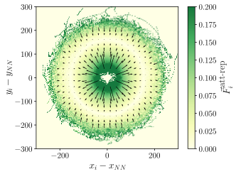
(a)

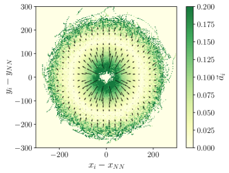
(b)

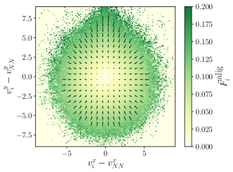
(c)

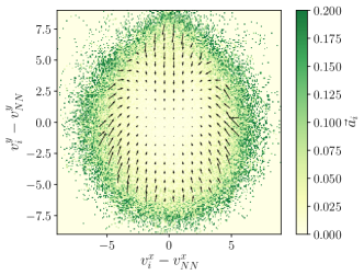
(d)

Figure 1: Attraction-repulsion and alignment force maps for the standard model. The force maps are able to recover qualitatively the behaviour of the corresponding forces. Average (a) attraction-repulsion force and (b) acceleration (attraction-repulsion force map) acting on an individual $i$ depending on its relative position with the nearest neighbour $NN$. We observe for small distances repulsion, for intermediate distances no net force and for large distances attraction. Average (c) alignment force and (d) acceleration (alignment force map) acting on an individual $i$ depending on its relative velocity with the nearest neighbour $NN$. In all plots, the $y$-axis is along the direction of motion of the focal individual, the colormap displays the modulus of the force and the arrows its components. We employ values for all focal individuals and time steps in the simulation.

Attraction-repulsion force map

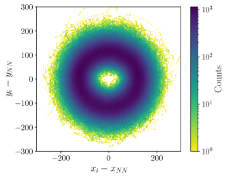
(a)

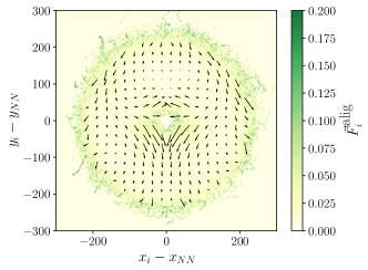
(b)

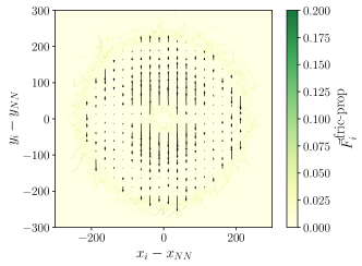
(c)

Figure S7: (a) Counts, (b) average alignment and (c) average friction-propulsion force acting on an individual $i$ depending on its relative position with nearest neighbour $NN$ for the standard model. The $y$-coordinate is along the direction of motion of the individual.

This force map was introduced both by Katz et al. [16] and Herbert-Read et al. [17]. It obtains the attraction and repulsion forces from the average acceleration $\vec{a}_{i}$ of an individual $i$ as a function of its position relative to the nearest neighbour $NN$, $\vec{x}_{i}-\vec{x}_{NN}$, assuming this neighbour dominates the interaction. We can demonstrate it with a simple model of schooling fish, which we refer as standard model. In this model individuals interact with some social forces, described by attraction-repulsion and alignment terms, and respond to some individual forces, represented by a friction-propulsion term to drive the motion and noise (for more details see Methods). Employing simulations of the model, we display in Fig. 1a the average attraction-repulsion force acting on a focal individual depending on its position relative to the the nearest neighbour. We use values for all focal individuals and time steps (counts are shown in Supplementary Fig. S7a). The components of the force are displayed with arrows and the modulus with the colormap. The $y$-coordinate is oriented along the direction of motion of the focal individual. We observe for near distances arrows point outwards, indicating the focal fish experiences a repulsive force away from the neighbour. For intermediate distances there is an area with no net force (the equilibrium distance). Finally, for far away distances arrows point inwards, signaling an attractive force towards the neighbour. Now in Fig. 1b we display the attraction-repulsion force map given by the average acceleration for an individual depending on its relative position with the nearest neighbour. Indeed, we observe it recovers satisfactorily the attraction-repulsion force. This procedure works adequately because other forces in this representation have practically negligible effects (Supplementary Fig. S7b and c).

We note previous works on the attraction-repulsion force map employed the reversed coordinates $\vec{x}_{NN}-\vec{x}_{i}$, but they typically separated the acceleration components in different plots and did not display the force with arrows (except in [20]). Because here instead we display the force as a vector, we find more natural to represent it analogously to a force field from physics, where the force at a point indicates the force a particle would feel at that point. Furthermore, we also want to remark that, in absence of other forces, a trajectory observed in the force map is more complex than just following the direction of the arrows, as there will be rotations caused by the $y$-axis pointing towards the direction of motion of the focal individual.

Alignment force map

Previous works used force maps for the alignment force that depend on angular differences as well as on relative positions, which make the alignment force more difficult to disentangle from the attraction and repulsion forces. Here instead we introduce a more natural force map for alignment in Cartesian coordinates obtained from calculating the average acceleration $\vec{a}_{i}$ of an individual $i$ as a function of its relative velocity with the nearest neighbour $NN$, $\vec{v}_{i}-\vec{v}_{NN}$. This approach is directly inspired from the expression of the alignment force between neighbours in our standard model (see Eq. 2 in Methods).

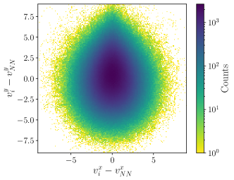
(a)

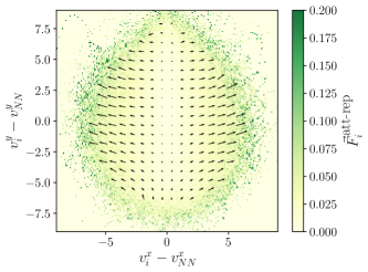
(b)

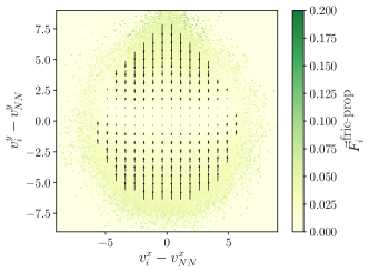
(c)

Figure S8: (a) Counts, (b) average attraction-repulsion and (c) average friction-propulsion force acting on an individual $i$ depending on its relative velocity with the nearest neighbour $NN$ for the standard model. The $y$-coordinate is along the direction of motion of the individual.

In Fig. 1c we show the average alignment force acting on a focal individual depending on its relative velocity with the nearest neighbour for the standard model. We employ values for all focal individuals and time steps (counts are shown in Supplementary Fig. S8a). The components of the force are displayed with arrows and the modulus with the colormap. The $y$-coordinate is oriented along the direction of motion of the focal individual. We observe the force vectors point inwards and increase with the velocity differences. This results in the force term decreasing the relative velocity and aligning the velocity of the focal individual with that of its neighbour. In Fig. 1d we show the alignment force map given by the average acceleration in this representation. This force map also recovers successfully the qualitative behaviour of the alignment force between an individual and a neighbour. Again, this works because other forces of the model in this representation have small contributions (Supplementary Fig. S8b and c).

Experimental force maps

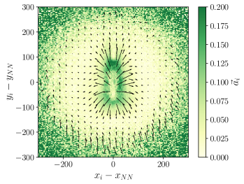
(a)

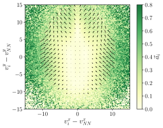
(b)

Figure 2: Force maps for the experimental data: (a) attraction-repulsion and (b) alignment force map. While the attraction-repulsion force map is similar to the standard model, the alignment force map displays a striking different behaviour: in the lower-half region arrows point inwards indicating alignment but in the upper-half region arrows point outwards indicating anti-alignment.

Equipped with the force maps technique outlined above, we are now able to explore experimental data of schooling fish. With this purpose, we analyze the motion of $N=39$ individuals of the species black neon tetra Hyphessobrycon herbertaxelrodi swimming freely in an experimental tank (see Methods for experimental details).

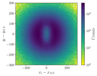
(a)

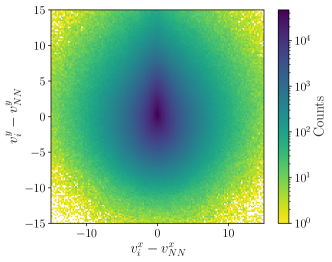
(b)

Figure S9: Counts for (a) attraction-repulsion and (b) alignment force maps for the experimental data.

We start with the attraction-repulsion force map in Fig. 2a (the counts of the force map are shown in Supplementary Fig. S9a). We see this force map has a similar qualitative behaviour to the attraction-repulsion force for the standard model (Fig. 1a), with repulsion for short distances, no net force for intermediate distances and attraction at large distances.

Now we turn our attention to the alignment force map obtained from experimental data, displayed in Fig. 2b (the counts are shown in Supplementary Fig. S9b). Contrary to the alignment force from the standard model (Fig. 1c), we can identify two qualitatively different behaviours depending on the sign of the difference of velocities between an individual and its nearest neighbour in the direction of motion of the individual ($y$-axis). If the neighbour is moving at faster speeds than the individual (lower-half part), we observe alignment interactions with the acceleration pointing inwards. However, when the neighbour moves at slower speeds than the individual (upper-half part), the acceleration points outwards and indicates a surprising anti-alignment interaction, with fish turning away from neighbours.

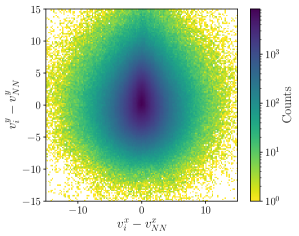
(a)

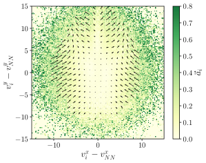
(b)

Figure S10: Alignment force maps for experimental data for a smaller number of fish $N=8$.

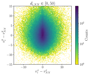
(b)

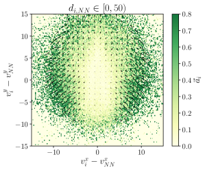
(c)

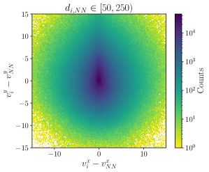
(d)

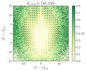
(e)

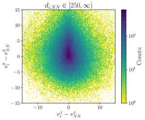
(f)

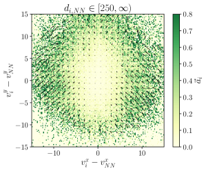
(g)

Figure S11: (a) Distribution of distances between nearest neighbours $d_{i,NN}$ and (b)-(g) alignment force maps for different $d_{i,NN}$ for the experimental data.

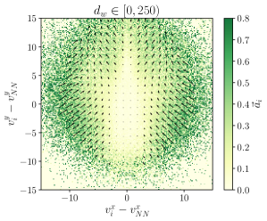
(c)

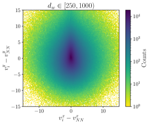
(d)

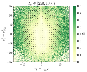
(e)

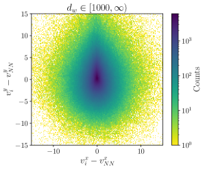
(f)

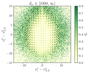
(g)

Figure S12: (a) Distribution of minimum distances to the walls $d_{w}\equiv\min(x,L-x,y,L-y)$, for $L$ the side of the tank, and (b)-(g) alignment force maps for different $d_{w}$ of the individual $i$ for the experimental data.

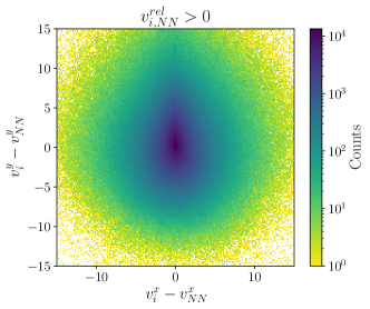
(a)

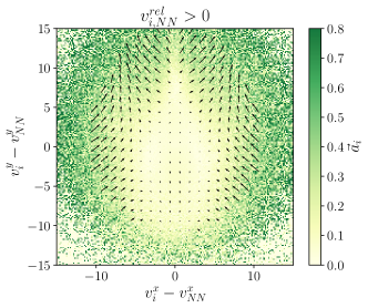
(b)

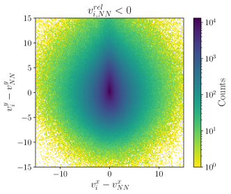
(c)

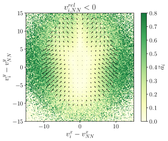
(d)

Figure S13: Alignment force maps for different velocity differences between an individual $i$ and its nearest neighbour $NN$ projected along their relative position direction $v_{i,NN}^{rel}\equiv(\vec{v}_{NN}-\vec{v}_{i})\cdot\hat{x}_{i,NN}$ for the experimental data: (a), (b) $v_{i,NN}^{rel}>0$ with the individual approaching the neighbour and (c), (d) $v_{i,NN}^{rel}<0$ with the individual moving away from the neighbour. We notice when the neighbour is approaching the individual ($v_{i,NN}^{rel}<0$) the alignment region is slightly stronger.

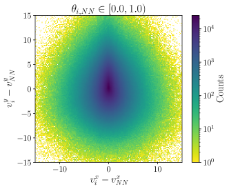
(a)

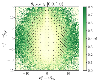
(b)

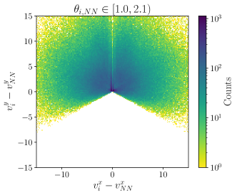
(c)

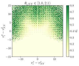
(d)

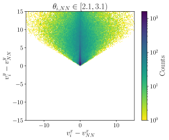
(e)

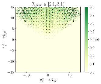
(f)

Figure S14: Alignment force maps for different heading orientations $\theta_{i,NN}$ between an individual $i$ and its nearest neighbour $NN$ for the experimental data.

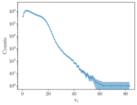
(a)

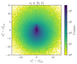
(b)

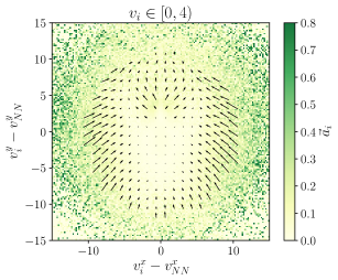
(c)

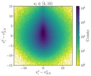
(d)

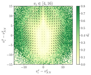
(e)

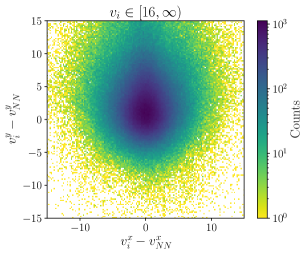
(f)

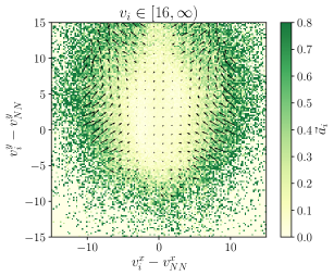
(g)

Figure S15: (a) Distribution of individual speeds $v_{i}$ and (b)-(g) alignment force maps for different $v_{i}$ for the experimental data. Notice how the strength of the force increases with the speed of the individual and the anti-alignment region shifts to the front. The error band in (a) is calculated from the standard deviation of a Bernoulli distribution with the probability given by the fraction of counts in each bin.

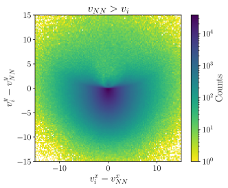
(a)

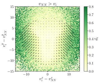
(b)

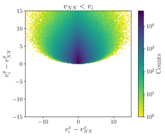
(c)

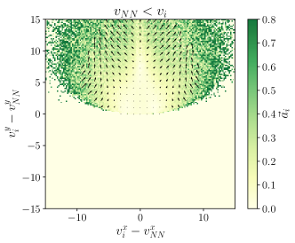
(d)

Figure S16: Alignment force maps for different relative velocities between the neighbour and the individual for the experimental data. They essentially occupy excluded regions in the force map.

We find that the qualitative behaviour of the alignment and anti-alignment regions in the alignment force map is robust against a variety of factors: different number of fish (Supplementary Fig. S10); different distances between neighbours (Supplementary Fig. S11), which tests for possible effects originating from the attraction or repulsion regimes in the attraction-repulsion force; different distances to the tank walls (Supplementary Fig. S12), which discards possible interactions with the walls; for the case the fish is approaching or moving away from the neighbour (Supplementary Fig. S13); for different heading orientations between the fish and its neighbour (Supplementary Fig. S14); and for different velocities of the focal individual (Supplementary Fig. S15). Only when differentiating the case where the neighbour moves at faster or slower speeds (Supplementary Fig. S16), we observe exclusively alignment or anti-alignment interactions in the expected regions of the map.

Explicit anti-alignment model

We find the standard model of schooling fish reproduces properly the attraction-repulsion force map in the experimental data of schooling fish, but is unable to account for the alignment force map. To correct this, we now consider a model variation implementing explicitly the alignment force observed experimentally. We do so by defining an alignment force given by an interpolation of the values in the experimental alignment force map, which is previously smoothed with a Gaussian filter of window $\sigma=2$ and with a cut-off for velocity differences larger than $23$. All other forces and parameters are kept the same as in the previous section.

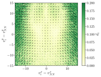
(a)

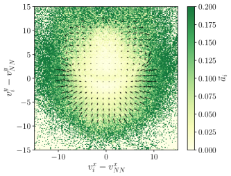
(b)

Figure 3: Model variations with alignment and anti-alignment regions in the alignment force map. Alignment force maps for (a) the explicit anti-alignment model and (b) the selective interactions model.

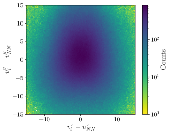
(a)

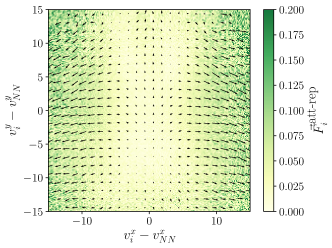
(b)

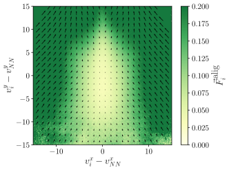
(c)

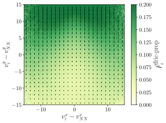
(d)

Figure S17: (a) Counts, (b) average attraction-repulsion, (c) average alignment and (d) average friction-propulsion force acting on an individual $i$ depending on its relative velocity with the nearest neighbour $NN$ for the explicit anti-alignment model.

Despite the model reproduces qualitatively the expected alignment force map (Fig. 3a and Supplementary Fig. S17), the dynamics is unrealistic. When an individual is moving faster than its neighbours, it is located in the anti-alignment region of the force map and the explicit anti-alignment force causes the individual to accelerate in the forward direction, which in the absence of other forces will result in an even larger speed. This behaviour is observed in the simulations of the model (see Supplementary Video S3), where some individuals acquire large speeds and move towards the front of the group. However, this is not found in the experimental data and there is no biological motivation for fast fish to waste energy by increasing their speed further.

Selective interactions model

The non-physical and non-biological features of the explicit anti-alignment model suggest that the anti-alignment region observed in the alignment force map of the experimental data may not originate from an explicit anti-alignment rule, but it could instead emerge from some other interaction that appears effectively as an anti-alignment force.

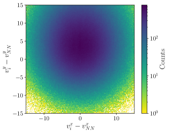
(a)

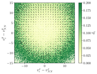
(b)

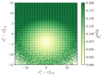
(c)

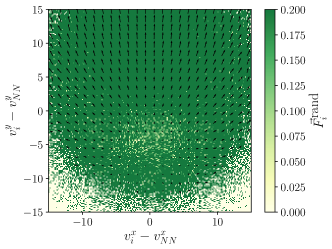
(d)

Figure S18: (a) Counts, (b) average acceleration (alignment force map), (c) average alignment force and (d) average persistent random force acting on an individual $i$ depending on its relative velocity with the nearest neighbour $NN$ for the standard model with a persistent random force. Here we use an individual has a probability rate $r=1/20$ to switch off the social forces and experience a persistent random force of amplitude $A=1.5$ for a time $\tau=5$. The persistent random force appears as an effective anti-alignment force with arrows pointing outwards. However, in this regime the alignment force dominates and the acceleration is displayed with alignment with arrows pointing inwards.

To explore this idea, we first study the effect of a persistent random force in the alignment force map. We propose a variation of the standard model, in which individuals have some probability rate $r$ to switch off their social interactions and feel instead a persistent force in a fixed random direction with a given amplitude $A$ for some time $\tau$. Biologically, this can be motivated as an individual fish may decide to follow private information based on environmental cues and temporarily ignore social cues. Depending on the relative strength of the persistent random force compared to the alignment force, we observe two different outcomes. When the alignment force dominates the persistent random force, we obtain an alignment force map that is still full alignment (Supplementary Fig. S18b). However, the persistent random force contributes to the total force with anti-alignment (Supplementary Fig. S18d). We can understand this as in a group with overall high directional alignment, a persistent “private” force acting temporarily in a fixed random direction will tend to make the focal fish turn away from their neighbour’s direction and appear effectively as an anti-alignment interaction. Naively, one could expect that in the regime when the persistent random force dominates the alignment force, the resulting alignment force map would be anti-alignment. However, that is not the case as there is not anymore ordered collective motion and the force map is essentially noise.

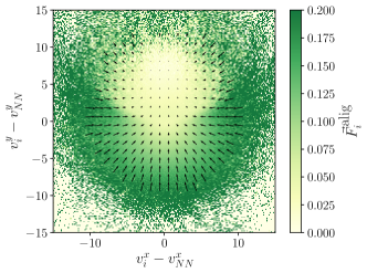
(c)

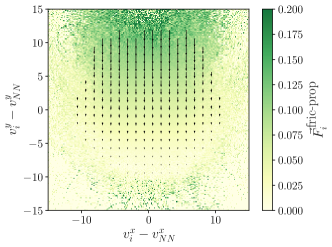
(d)

Figure S19: (a) Counts, (b) average attraction-repulsion, (c) average alignment and (d) average friction-propulsion force acting on an individual $i$ depending on its relative velocity with the nearest neighbour $NN$ for the selective interactions model. Here the attraction-repulsion force for slower nearest neighbours acts as an effective anti-alignment force with arrows pointing outwards.

To connect this idea with the observed experimental alignment force map, we propose another variation of the standard model, a selective interactions model where individuals pay attention primarily to neighbours exhibiting strong movement cues. We assume that individuals interact socially with neighbours that move at a speed larger than their own, and switch off social interactions with neighbours that move at a smaller speed (see Supplementary Video S4). The weights in the social interactions are calculated as in the standard model (see Methods) but considering only faster neighbours. We display the alignment force map in Fig. 3b (the counts are shown in Supplementary Fig. S19). We see this model reproduces the features observed in the experimental data, with alignment for faster neighbours and anti-alignment for slower neighbours. The emergence of anti-alignment for slower nearest neighbours in this model can be traced back to the attraction-repulsion force (see Supplementary Fig. S19). Although this force is switched off for slower neighbours, the focal individual will continue to interact with other non-nearest faster neighbours. Thus, when we construct the alignment force map for the slower nearest neighbours, the actual dynamics of the focal agent is driven by attraction to farther away neighbours, which may be located at random relative positions. This force then can act in any direction and, therefore, appears effectively as a persistent random force. As we found previously, this results in individuals on average turning away from their nearest neighbour and displaying apparently an anti-alignment interaction.

Comparison of observables in the models

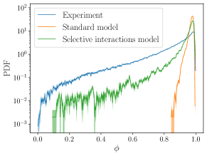
(a)

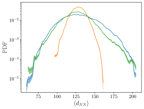
(b)

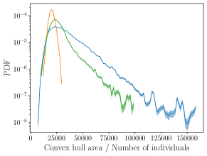
(c)

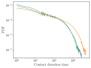
(d)

Figure 4: The selective interactions model is more similar to the experimental data than the standard model for a set of observables. Probability density functions (PDF) of (a) polarization $\phi$, (b) instantaneous average nearest neighbour distance $\left<d_{NN}\right>$, (c) area of the convex hull normalized by the number of individuals and (d) contact duration time between Voronoi neighbours. The error bands are calculated from the standard deviation of a Bernoulli distribution, with the probability given by the fraction of counts in each bin.

Our analysis based on the alignment force map suggests the selective interactions model as a more accurate depiction of the experimental data than the standard model. Here, we extend our investigation by comparing the models and the experimental data with a set of observables (Fig. 4). The polarization $\phi$,

$$\phi\equiv\left|\frac{1}{N}\sum_{i}\frac{\vec{v}}{v}\right|,$$

is a measure of the group order that tends to $1$ if all individuals move in the same direction, and decreases when they move in increasingly different directions. The nearest neighbour distance averaged for all individuals $\left<d_{NN}\right>$ is a measure of the cohesiveness of the group. The convex hull of the group is defined as the smallest convex polygon that contains all individuals. Its area normalized by the number of individuals is a measure of the extension occupied by the group. The contact duration time between Voronoi neighbours is a measure of the persistence of the local neighbours structure.

The selective interactions model outperforms the standard model in its ability to reproduce the various experimental observables: it is on average less ordered by displaying a broad distribution of order parameter values (with more low polarization values); it exhibits a larger variability in the nearest neighbour distances (wider PDF), more extended groups (with higher values for the convex hull areas) and larger rates of neighbours shuffling (with shorter contact duration times of Voronoi neighbours).

Leadership and alignment

Our above results suggest that the features of the experimental alignment map may be explained by selective social interactions with faster individuals. In this section, we want to validate this hypothesis, connecting it to the possible presence of leader-follower relationships.

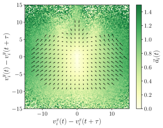
(a)

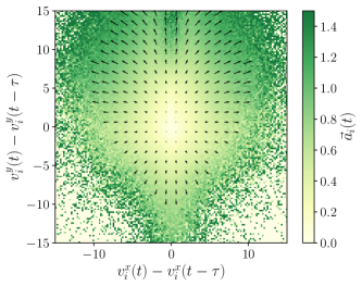
(b)

Figure 5: Alignment force maps for surrogate data of the experimental school with known leader-follower interactions. We compare the individual $i$ with itself at (a) positive and (b) negative delayed time $\tau=10$. When the delay is positive, the individual at present acts as a follower and we see pure alignment. When the delay is negative, the individual at present acts as a leader and we see pure anti-alignment.

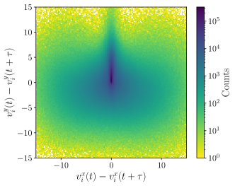
(a)

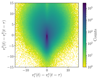
(b)

Figure S20: Counts for the alignment force maps for the experimental data comparing the individual at present with itself at a (a) positive and (b) negative delay with $\tau=10$.

We start by constructing surrogate data where we know a priori the flow of information between leaders and followers, and use the alignment force map to explore it. To achieve this, we use the following trick in the experimental data: for the focal individual we take the individual $i$ at the present time $t$, while for the neighbour we consider the same individual $i$ at a delayed time $t+\tau$. In the case of a positive delay $\tau$, the direction of the individual at present will follow that of the individual in the future after the delayed time, such that the individual at present can be interpreted as the follower within this pair. Now, when we observe the alignment force map for the individual at present (Fig. 5a and Supplementary Fig. S20), we find alignment in all regions. This suggests a follower aligns with a leader. In the case of a negative delay, we have the opposite situation and the direction of the individual at present is adopted by the individual in the past after the delayed time and thus the individual at present can be interpreted as the leader. In the alignment force map (Fig. 5b and Supplementary Fig. S20), this results in anti-alignment in all regions, i.e. a leader appears to anti-align with a follower. However, this does not necessarily imply explicit anti-alignment, but originates rather from the leader ignoring the follower and moving in a different direction.

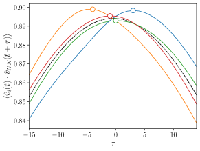
(a)

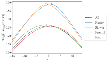
(b)

Figure 6: Relative speeds in neighbours describe better leadership in schooling fish than frontal distances along the direction of motion of the individual. Correlations in (a) the orientation and (b) speed (Pearson correlation coefficient $r$) between an individual $i$ and its nearest neighbour $NN$ at a delayed time $\tau$ for the experimental data. We filter for different states of the individual compared to the neighbour (see legend). The circle denotes the maximum of each line. We find correlations are higher for faster and slower individuals than frontal and rear individuals.

Extrapolating this analysis to the experimental alignment force map (Fig. 2b) hints to the idea that individuals act as leaders when moving faster than their neighbours (anti-alignment region), while they act as followers when moving slower than their neighbours (alignment region). We verify this idea by calculating correlations between the velocities of the individual and the nearest neighbour at a delayed time in the experimental data. We consider two types of correlations, in the orientation given by $\left<\hat{v}_{i}(t)\cdot\hat{v}_{NN}(t+\tau)\right>$ [23] (Fig. 6a) and in the speed given by the Pearson correlation coefficient $r(v_{i}(t),v_{NN}(t+\tau))$ [16] (Fig. 6b). In the presence of leadership interactions, a follower requires some time to react and copy the leader. This results in these correlations having a higher value at that delayed time, provided the frame rate is higher than the reaction time of the follower. If the maximum occurs for a positive delay $\tau$, this implies the individual is the leader. While for a negative delay, the individual is the follower. Moreover, the value of the maximum reflects the amount of information transmitted by the leadership flow. In particular, we are interested in studying correlations differentiating by the state of the individual. In blue and orange lines, we display the correlations performed for individuals faster and slower than their neighbour, respectively. Indeed, we see in both correlations that faster individuals have a maximum for positive delays, which means they are leaders. The opposite occurs with slower individuals, which act as followers. We also compare this measure of leadership with the commonly used measure of frontal distances along the direction of motion of the individual [23, 34], filtering for frontal and rear individuals (green and red lines). In fact, we find correlations have higher values for faster and slower individuals than for frontal and rear individuals, indicating leadership in neighbours is better described by relative speeds rather than with frontal distances along the direction of motion. Note also that the faster and slower curves are not necessarily symmetrical along the $y$-axis, as several individuals can have the same nearest neighbour. The same occurs for frontal and rear, but in addition, a frontal and rear individual in the direction of motion of the individual can also be frontal and rear respectively in the direction of motion of the neighbour.

Discussion

In this paper we have introduced a force map to study the alignment force. Using this force map together with the attraction-repulsion force map, we have been able to capture and distinguish the attraction-repulsion and alignment forces in a simple model of schooling fish. Applying it to experimental data, we found a robust signature of alignment of the focal individual with faster neighbours and anti-alignment with slower neighbours. Instead of explicit anti-aligning behavior, we suggest that the signatures of anti-alignment are the result of a selective attention mechanism, where fish pay less attention and, thus, have weaker interactions with slower neighbours. We were able to find support for this hypothesis by analysing the effective interactions in an agent-based model with selective alignment force. From this hypothesis, we were also able to build a connection between the alignment patterns and leadership interactions. We show that followers display only alignment force and leaders only anti-alignment force. We then verified in the experimental schooling fish that faster and slower individuals are leaders and followers respectively with their nearest neighbours. This measure of leadership is more statistically significant than the traditionally used in the literature of frontal distances along the direction of motion.

While previous research suggests that individual speeds play an important role in shaping collective movement, and that leader-follower interactions are mediated by speeds, it either considered average speeds [30, 28, 31, 32] or instantaneous absolute speeds of the neighbour [29]. Furthermore, the proposed mechanism is based on self-organization of individuals with different average speeds assuming homogeneous and constant social interactions [31, 32]. Our results reinforce the link between speed and leadership with completely different methods and by using a more restrictive concept, given by instantaneous speeds of the neighbour relative to the focal individual. But more importantly, we provide evidence for selective interactions based on relative speed of individuals, which was previously suggested in a model with escape and pursuit interactions [3]. This implies a dynamic modulation of social interactions, which not only amplifies the importance of individual speed, but also provides a mechanism for dynamic adaptation of leader-follower relationships on short time-scales independent of the average preferred speed of individuals.

If we interpret social interactions between individuals as a method to transfer information across the group, these results suggest higher relevance of information provided by faster moving individuals [29]. This makes biological sense as informed individuals acting on privately acquired information, such as perception of a predator or food, are expected to move at higher speeds [24]. However, here it should be also noted that faster movement cues, embedded in a background of slower moving ones, are also perceptually more salient [35].

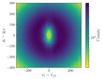
(a)

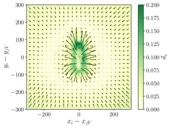
(b)

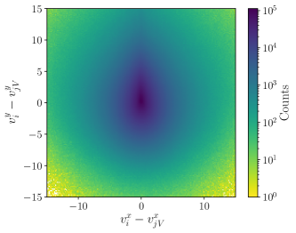
(c)

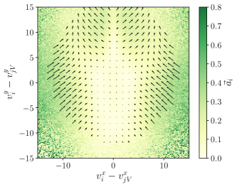
(d)

Figure S21: For Voronoi neighbours: (a) counts of the relative positions between neighbours, (b) attraction-repulsion force map, (c) counts of the relative velocities between neighbours and (d) alignment force map for the experimental data.

In the calculation of force maps, we considered only the relative position and velocity of a single, nearest neighbour. While this is supported by 1-2 influential neighbours identified in previous work on fish schools [17, 36], one could, in principle, also use the relative position and velocity of all Voronoi neighbours (Supplementary Fig. S21). While we observe partial screening of attractive interactions in the attraction-repulsion force map, the force maps with Voronoi neighbours resemble qualitatively the force maps with the nearest neighbour. This suggests that the nearest neighbour dominates the interactions. We also find support for this idea when we explored simulations of the standard model without weights and found more inadequate force maps with some screening effects.

Our results showcase how selective social interactions may lead to unexpected signatures at the level of averaged behavioral responses to social cues. It is of relevance for quantitative analysis of social interactions across taxa, as it demonstrates that extreme caution is needed when extracting behavioral algorithms from aggregated data such as force maps, in particular in the context of complex self-organized collective behaviors. Here, a combination of quantitative data as well as theoretical modelling taking into account properties and constraints of perception will provide deeper insights into social interactions and functional aspects of collective behavior with respect to transfer and distributed processing of information. More specifically, selective social interactions depending on relative speeds likely play an important role for different grouping phenomena [3], and provide an explicit mechanism on how speed may be a core variable at the individual level affecting the dynamics and the structure of animal collectives [31, 32, 37, 38].

Methods

Standard model

We consider a model of schooling fish in two-dimensions with $N$ individuals where each individual $i$ is subject to a total force $\vec{F}_{i}$ given by social forces, represented by attraction-repulsion $\vec{F}^{\text{att-rep}}_{i}$ and alignment $\vec{F}^{\text{alig}}_{i}$ forces, and individual forces, consisting of a friction-propulsion force $\vec{F}^{\text{fric-prop}}_{i}$ and noise $\vec{F}^{\text{noise}}_{i}$ that capture other unknown forces [39]:

$$\vec{F}_{i}=\vec{F}^{\text{att-rep}}_{i}+\vec{F}^{\text{alig}}_{i}+\vec{F}^{\text{fric-prop}}_{i}+\vec{F}^{\text{noise}}_{i}.$$

For simplicity, we use a first order approximation for the different force terms. Thus, the attraction-repulsion force acting on an individual $i$ due to the neighbour $j$ reads:

$$\vec{F}^{\text{att-rep}}_{ij}=-k\left(d_{ij}-d_{0}\right)\frac{\vec{x}_{i}-\vec{x}_{j}}{d_{ij}},$$ (1)

where $d_{0}$ is the equilibrium distance between neighbours, $d_{ij}=\left|\vec{x}_{j}-\vec{x}_{i}\right|$ is the distance between individuals $i$ and $j$, $\vec{x}_{i}$ is the position of individual $i$ and $k=k_{\text{rep}}$ for $d_{ij}\leq d_{0}$ and $k=k_{\text{att}}$ for $d_{ij}>d_{0}$. This force acts a restoring force towards the equilibrium distance between the neighbours.

The alignment force experienced by an individual $i$ due to its neighbour $j$ is given by [40]:

$$\vec{F}^{\text{alig}}_{ij}=-\mu(\vec{v}_{i}-\vec{v}_{j}),$$ (2)

where $\vec{v}_{k}$ are individual velocities. This force acts as a restoring force for the focal individual towards reaching the same speed and heading as its neighbour.

We use interactions with Voronoi neighbours, which are a good approximation to visual interaction networks [41], and we average the social forces, $\vec{F}^{\text{social}}_{ij}=\vec{F}^{\text{att-rep}}_{ij}+\vec{F}^{\text{alig}}_{ij}$, for the different neighbours with weights given by the inverse of their metric distance $d_{ij}$:

$$\vec{F}^{\text{social}}_{i}=\sum_{j}w_{ij}\vec{F}^{\text{social}}_{ij},$$

where $w_{ij}=\frac{1}{d_{ij}}$. With this choice of weights, closer neighbours exert more influence, a result observed in previous studies [17, 24, 42, 15].

For the individual forces, we use a friction-propulsion term [40]:

$$\vec{F}^{\text{fric-prop}}_{i}=-\frac{v_{i}-v_{0}}{\tau}\hat{v}_{i},$$

where $v_{0}$ is the fish preferred speed and $\tau$ is the speed relaxation time. This introduces a self-propulsion force for the fish to move with a speed around $v_{0}$, with $\tau$ being the typical timescale of velocity adaptation. The noise force corresponds to active fluctuations [43, 40], with independent noise terms acting on the direction of motion $\hat{v}_{i}$ and its perpendicular direction $\hat{\varphi}_{i}$:

$$\vec{F}^{\text{noise}}_{i}=\sigma_{v}\xi_{v}(t)\hat{v}_{i}+\sigma_{\varphi}\xi_{\varphi}(t)\hat{\varphi}_{i},$$

where $\xi(t)_{v}$ and $\xi_{\varphi}(t)$ are independent Gaussian white noise processes with $\langle\xi_{x}(t)\xi_{y}(t^{\prime})\rangle=\delta(t-t^{\prime})\delta_{xy}$.

We perform simulations integrating numerically the equations of motion in order to obtain the trajectory $\vec{x}_{i}$:

$$\vec{a}_{i}=\vec{F}_{i},$$

where $\vec{a}_{i}=\frac{d^{2}\vec{x}_{i}}{dt^{2}}$ is the acceleration, and we work with units of mass $m=1$. The values of the parameters in the model, shown in Table 1, have been selected in order to provide similar results to our experimental data, as described in the Supplementary Information.

Here we work with $N=39$ individuals, matching the maximum number of fish in our experimental data. We solve the stochastic differential equation with the Euler-Maruyama algorithm [44]. We choose random initial positions and velocities for the individuals such that the extension of the group and speeds are similar to the experimental school, but each individual is oriented uniformly at random. We discard as transient the first 1000 frames. We show in Supplementary Video S2 trajectories generated by the standard model.

Table 1: Parameter values used in the standard model in units of pixels and frames.

Parameters	Values
$k_{\text{rep}}$	0.005
$k_{\text{att}}$	0.002
$d_{0}$	160
$\mu$	0.03
$v_{0}$	6
$\tau$	80
$\sigma_{v}$	0.5
$\sigma_{\varphi}$	0.2

Experimental data

Experiments, performed at the Scientific and Technological Centers UB (CCiTUB), University of Barcelona (Spain), were made with black neon tetra Hyphessobrycon herbertaxelrodi, a small freshwater fish of average body length 2.5 cm that has a strong tendency to form compact and highly polarized schools [45]. Experiments consisted in $N$ individuals freely swimming in a square tank of 100 cm of side and 5 cm of depth. Videos of the fish movement were recorded at 50 frames per second with a resolution of 5312×2988 pixels. Digitized individual trajectories were obtained from the video recordings using the software idtracker.ai [46]. Invalid values returned by the program caused by occlusions were corrected in a supervised way, semi-automatically interpolating with spline functions (now incorporated in the Validator tool from version 5 of idtracker.ai). For better accuracy, we projected the trajectories in the plane of the fish movement, warping the tank walls of the image into a proper square (see Supplementary Information). Moreover, we smooth the trajectories with a Gaussian filter with $\sigma=2$, truncating the filter at $5\sigma$. We calculate the velocities and accelerations from the Gaussian filter using derivatives of the Gaussian kernel. We work in units of pixels for distances and frames for times, which are the natural units to compare against the experimental resolution error.

We performed experiments with $N=39$ fish (2 recordings of 60 minutes) and $N=8$ (6 recordings of 30 minutes). In Supplementary Video S1 we show a rendering of of the evolution of the $N=39$ school with the digitized trajectories overlapped with the real video.

Author contributions

A.P., P.B., M.C.M., R.P.-S. and P.R. designed the study. E.G. and J.T. acquired the empirical data. J.T. and A.P. processed the empirical data. A.P. analysed the empirical data and performed the numerical simulations. A.P., P.B., M.C.M., R.P.-S. and P.R. analysed the results. A.P., R.P.-S. and P.R. wrote the paper. All authors commented on the manuscript.

Competing interests

The authors declare no competing interests.

SUPPLEMENTARY INFORMATION
 

Standard model parameters selection

Our aim with the standard model is to describe with few simple linear terms the qualitative behaviour of schooling fish, rather than matching quantitative aspects. In this line of thought, instead of fitting the parameters to some goal function we use values at the expected order of magnitude comparing with the experimental data of schooling fish. We also confirmed that our qualitative results remain unchanged upon varying of these parameters.

The constants $k_{\text{rep}}$ and $k_{\text{att}}$ are chosen by comparing the pairwise attraction-repulsion force (Eq. 1) to the attraction-repulsion force map (Fig. 2a). In particular, we find $k_{\text{rep}}>k_{\text{att}}$, as fish may prioritize repulsion to attraction [6].

The equilibrium distance $d_{0}$ is fixed such that numerical simulations match the average distance between nearest neighbors observed in experimental data (Fig. 4b).

The alignment constant $\mu$ is taken analogously comparing the pairwise alignment force map (Eq. 2) to the alignment region in the alignment force map (Fig. 2b).

The fish preferred speed $v_{0}$ is chosen from the average individual speeds (Supplementary Fig. S15a).

The time scale $\tau$ is obtained from the average time period of the the burst-and-coast oscillations observed in the individual speeds.

The noise constants $\sigma_{v}$ and $\sigma_{\phi}$ are chosen such that the explored regions in the force maps are comparable to the experimental data. Studying the PDFs of acceleration differences $\delta\vec{a}_{i}(t)\equiv\vec{a}_{i}(t+1)-\vec{a}_{i}(t)$, we found $\sigma_{v}>\sigma_{\phi}$, which we also preserve in the simulations.

Trajectories projection

The perspective of the camera was not exactly perpendicular to the plane of motion of the fish. For better accuracy, we project the calculated trajectories to the plane parallel to the bottom of the tank. In order to do this, first we look for the pixels of the corners of the tank walls in the videos and calculate the height and base of the corresponding rectangle in pixels. Because the tank is actually a square, we define the side of the tank $L$ in pixels as the average value of the base and height of the rectangle image. We define the new tank corners: $(0,0)$, $(0,L)$, $(L,0)$ and $(L,L)$ and we calculate the perspective transform matrix $M$ from the original and new tank corners using the function getPerspectiveTransform() from the OpenCV library [47]. Finally, we obtain the transformed trajectories $(x^{\prime},y^{\prime})$ applying a perspective transformation to the original trajectories $(x,y)$, as explained in the OpenCV documentation:

$$(x^{\prime},y^{\prime})=\left(\frac{M_{11}x+M_{12}y+M_{13}}{M_{31}x+M_{32}y+M_{33}},\frac{M_{21}x+M_{22}y+M_{23}}{M_{31}x+M_{32}y+M_{33}}\right).$$

Rendering of the movement of fish in a experimental school of size $N=39$, overlapped with the digitized trajectories, displayed in blue.

Dynamics for the standard model of schooling fish. The reference frame is comoving with the center of mass of the group. The position of the individuals and their velocities are shown in blue. We also display the different force terms in the model (legend): the alignment force (magenta), the attraction-repulsion force (red) and the friction-propulsion force (cyan). Each individual is linked with an edge to their Voronoi neighbours: in blue when they have attraction and in orange when they have repulsion.

Dynamics for the explicit anti-alignment model. The reference frame is comoving with the center of mass of the group. The position of the individuals and their velocities are shown in blue. We also display the different force terms in the model (legend): the alignment force (magenta), the attraction-repulsion force (red) and the friction-propulsion force (cyan). Each individual is linked with an edge to their Voronoi neighbours: in blue when they have attraction and in orange when they have repulsion.

Dynamics for the selective interactions model. The reference frame is comoving with the center of mass of the group. The position of the individuals and their velocities are shown in blue when they interact with other individuals and in black when they do not interact. We also display the different force terms in the model (legend): the alignment force (magenta), the attraction-repulsion force (red) and the friction-propulsion force (cyan). Each individual is linked to their Voronoi neighbours with an edge reaching half their distance if they are interacting: in blue when they have attraction and in orange when they have repulsion.

(a)

(a)

(b)

(a)

(b)

References

- Sumpter [2010] D. J. T. Sumpter, Collective Animal Behavior (Princeton University Press, 2010).
- Vicsek and Zafeiris [2012] T. Vicsek and A. Zafeiris, Collective motion, Physics Reports 517, 71 (2012).
- Romanczuk et al. [2009] P. Romanczuk, I. D. Couzin, and L. Schimansky-Geier, Collective Motion due to Individual Escape and Pursuit Response, Physical Review Letters 102, 010602 (2009).
- Herbert-Read [2016] J. E. Herbert-Read, Understanding how animal groups achieve coordinated movement, Journal of Experimental Biology 219, 2971 (2016).
- Reynolds [1998] C. W. Reynolds, Flocks, herds, and schools: A distributed behavioral model, in Seminal Graphics (ACM, New York, NY, USA, 1998) pp. 273–282.
- Couzin et al. [2002] I. D. Couzin, J. Krause, R. James, G. D. Ruxton, and N. R. Franks, Collective Memory and Spatial Sorting in Animal Groups, Journal of Theoretical Biology 218, 1 (2002).
- Strömbom [2011] D. Strömbom, Collective motion from local attraction, Journal of Theoretical Biology 283, 145 (2011).
- Ferrante et al. [2013] E. Ferrante, A. E. Turgut, M. Dorigo, and C. Huepe, Elasticity-Based Mechanism for the Collective Motion of Self-Propelled Particles with Springlike Interactions: A Model System for Natural and Artificial Swarms, Physical Review Letters 111, 268302 (2013).
- Barberis and Peruani [2016] L. Barberis and F. Peruani, Large-Scale Patterns in a Minimal Cognitive Flocking Model: Incidental Leaders, Nematic Patterns, and Aggregates, Physical Review Letters 117, 248001 (2016).
- Bastien and Romanczuk [2020] R. Bastien and P. Romanczuk, A model of collective behavior based purely on vision, Science Advances 6, eaay0792 (2020).
- Strömbom and Tulevech [2022] D. Strömbom and G. Tulevech, Attraction vs. Alignment as Drivers of Collective Motion, Frontiers in Applied Mathematics and Statistics 7 (2022).
- Lukeman et al. [2010] R. Lukeman, Y.-X. Li, and L. Edelstein-Keshet, Inferring individual rules from collective behavior, Proceedings of the National Academy of Sciences 107, 12576 (2010).
- Calovi et al. [2018] D. S. Calovi, A. Litchinko, V. Lecheval, U. Lopez, A. P. Escudero, H. Chaté, C. Sire, and G. Theraulaz, Disentangling and modeling interactions in fish with burst-and-coast swimming reveal distinct alignment and attraction behaviors, PLOS Computational Biology 14, e1005933 (2018).
- Escobedo et al. [2020] R. Escobedo, V. Lecheval, V. Papaspyros, F. Bonnet, F. Mondada, C. Sire, and G. Theraulaz, A data-driven method for reconstructing and modelling social interactions in moving animal groups, Philosophical Transactions of the Royal Society B: Biological Sciences 375, 20190380 (2020).
- Heras et al. [2019] F. J. H. Heras, F. Romero-Ferrero, R. C. Hinz, and G. G. de Polavieja, Deep attention networks reveal the rules of collective motion in zebrafish, PLOS Computational Biology 15, e1007354 (2019).
- Katz et al. [2011] Y. Katz, K. Tunstrom, C. C. Ioannou, C. Huepe, and I. D. Couzin, Inferring the structure and dynamics of interactions in schooling fish, Proceedings of the National Academy of Sciences 108, 18720 (2011).
- Herbert-Read et al. [2011] J. E. Herbert-Read, A. Perna, R. P. Mann, T. M. Schaerf, D. J. T. Sumpter, and A. J. W. Ward, Inferring the rules of interaction of shoaling fish, Proceedings of the National Academy of Sciences 108, 18726 (2011).
- Pettit et al. [2013] B. Pettit, A. Perna, D. Biro, and D. J. T. Sumpter, Interaction rules underlying group decisions in homing pigeons, Journal of The Royal Society Interface 10, 20130529 (2013).
- Herbert-Read et al. [2017] J. E. Herbert-Read, E. Rosén, A. Szorkovszky, C. C. Ioannou, B. Rogell, A. Perna, I. W. Ramnarine, A. Kotrschal, N. Kolm, J. Krause, and D. J. T. Sumpter, How predation shapes the social interaction rules of shoaling fish, Proceedings of the Royal Society B: Biological Sciences 284, 20171126 (2017).
- Zienkiewicz et al. [2018] A. K. Zienkiewicz, F. Ladu, D. A. Barton, M. Porfiri, and M. D. Bernardo, Data-driven modelling of social forces and collective behaviour in zebrafish, Journal of Theoretical Biology 443, 39 (2018).
- Mudaliar and Schaerf [2020] R. K. Mudaliar and T. M. Schaerf, Examination of an averaging method for estimating repulsion and attraction interactions in moving groups, PLOS ONE 15, e0243631 (2020).
- Zafeiris and Vicsek [2018] A. Zafeiris and T. Vicsek, Why We Live in Hierarchies?: A Quantitative Treatise, SpringerBriefs in Complexity (Springer International Publishing, Cham, 2018).
- Nagy et al. [2010] M. Nagy, Z. Ákos, D. Biro, and T. Vicsek, Hierarchical group dynamics in pigeon flocks, Nature 464, 890 (2010).
- Rosenthal et al. [2015] S. B. Rosenthal, C. R. Twomey, A. T. Hartnett, H. S. Wu, and I. D. Couzin, Revealing the hidden networks of interaction in mobile animal groups allows prediction of complex behavioral contagion, Proceedings of the National Academy of Sciences 112, 4690 (2015).
- Orange and Abaid [2015] N. Orange and N. Abaid, A transfer entropy analysis of leader-follower interactions in flying bats, The European Physical Journal Special Topics 224, 3279 (2015).
- Bumann and Krause [1993] D. Bumann and J. Krause, Front Individuals Lead in Shoals of Three-Spined Sticklebacks (Gasterosteus Aculeatus) and Juvenile Roach (Rutilus Rutilus), Behaviour 125, 189 (1993).
- Crosato et al. [2018] E. Crosato, L. Jiang, V. Lecheval, J. T. Lizier, X. R. Wang, P. Tichit, G. Theraulaz, and M. Prokopenko, Informative and misinformative interactions in a school of fish, Swarm Intelligence 12, 283 (2018).
- Gimeno et al. [2018] E. Gimeno, F. S. Beltran, R. Dolado, and V. Quera, Leadership and collective motion in black neon tetra schools: Does the task matter?, Marine and Freshwater Behaviour and Physiology 51, 359 (2018).
- Romero-Ferrero et al. [2023] F. Romero-Ferrero, F. J. H. Heras, D. Rance, and G. G. de Polavieja, A study of transfer of information in animal collectives using deep learning tools, Philosophical Transactions of the Royal Society B: Biological Sciences 378, 20220073 (2023).
- Pettit et al. [2015] B. Pettit, Z. Ákos, T. Vicsek, and D. Biro, Speed Determines Leadership and Leadership Determines Learning during Pigeon Flocking, Current Biology 25, 3132 (2015).
- Jolles et al. [2017] J. W. Jolles, N. J. Boogert, V. H. Sridhar, I. D. Couzin, and A. Manica, Consistent Individual Differences Drive Collective Behavior and Group Functioning of Schooling Fish, Current Biology 27, 2862 (2017).
- Jolles et al. [2020a] J. W. Jolles, N. Weimar, T. Landgraf, P. Romanczuk, J. Krause, and D. Bierbach, Group-level patterns emerge from individual speed as revealed by an extremely social robotic fish, Biology Letters 16, 20200436 (2020a).
- Bödeker et al. [2010] H. U. Bödeker, C. Beta, T. D. Frank, and E. Bodenschatz, Quantitative analysis of random ameboid motion, EPL (Europhysics Letters) 90, 28005 (2010).
- Chen et al. [2016] D. Chen, T. Vicsek, X. Liu, T. Zhou, and H.-T. Zhang, Switching hierarchical leadership mechanism in homing flight of pigeon flocks, EPL (Europhysics Letters) 114, 60008 (2016).
- Ivry and Cohen [1992] R. B. Ivry and A. Cohen, Asymmetry in visual search for targets defined by differences in movement speed, Journal of Experimental Psychology: Human Perception and Performance 18, 1045 (1992).
- Jiang et al. [2017] L. Jiang, L. Giuggioli, A. Perna, R. Escobedo, V. Lecheval, C. Sire, Z. Han, and G. Theraulaz, Identifying influential neighbors in animal flocking, PLOS Computational Biology 13, e1005822 (2017).
- Jolles et al. [2020b] J. W. Jolles, A. J. King, and S. S. Killen, The Role of Individual Heterogeneity in Collective Animal Behaviour, Trends in Ecology & Evolution 35, 278 (2020b).
- Klamser and Romanczuk [2021] P. P. Klamser and P. Romanczuk, Collective predator evasion: Putting the criticality hypothesis to the test, PLOS Computational Biology 17, e1008832 (2021).
- Romanczuk et al. [2012] P. Romanczuk, M. Bär, W. Ebeling, B. Lindner, and L. Schimansky-Geier, Active Brownian particles: From individual to collective stochastic dynamics, The European Physical Journal Special Topics 202, 1 (2012).
- Klamser et al. [2021] P. P. Klamser, L. Gómez-Nava, T. Landgraf, J. W. Jolles, D. Bierbach, and P. Romanczuk, Impact of Variable Speed on Collective Movement of Animal Groups, Frontiers in Physics 9 (2021).
- Strandburg-Peshkin et al. [2013] A. Strandburg-Peshkin, C. R. Twomey, N. W. Bode, A. B. Kao, Y. Katz, C. C. Ioannou, S. B. Rosenthal, C. J. Torney, H. S. Wu, S. A. Levin, and I. D. Couzin, Visual sensory networks and effective information transfer in animal groups, Current Biology 23, R709 (2013).
- Sosna et al. [2019] M. M. G. Sosna, C. R. Twomey, J. Bak-Coleman, W. Poel, B. C. Daniels, P. Romanczuk, and I. D. Couzin, Individual and collective encoding of risk in animal groups, Proceedings of the National Academy of Sciences 116, 20556 (2019).
- Romanczuk and Schimansky-Geier [2011] P. Romanczuk and L. Schimansky-Geier, Brownian Motion with Active Fluctuations, Physical Review Letters 106, 230601 (2011).
- Toral and Colet [2014] R. Toral and P. Colet, Stochastic Numerical Methods: An Introduction for Students and Scientists (John Wiley & Sons, 2014).
- Gimeno et al. [2016] E. Gimeno, V. Quera, F. S. Beltran, and R. Dolado, Differences in shoaling behavior in two species of freshwater fish (Danio rerio and Hyphessobrycon herbertaxelrodi)., Journal of Comparative Psychology 130, 358 (2016).
- Romero-Ferrero et al. [2019] F. Romero-Ferrero, M. G. Bergomi, R. C. Hinz, F. J. H. Heras, and G. G. de Polavieja, Idtracker.ai: Tracking all individuals in small or large collectives of unmarked animals, Nature Methods 16, 179 (2019).
- Bradski [2000] G. Bradski, The OpenCV Library, Dr. Dobb’s Journal: Software Tools for the Professional Programmer 25 (2000).
Acknowledgements.
A.P. acknowledges a fellowship from the Secretaria d’Universitats i Recerca of the Departament d’Empresa i Coneixement, Generalitat de Catalunya, Catalonia, Spain and a scholarship Erasmus+. P.B. and P.R. acknowledge funding by the Deutsche Forschungsgemeinschaft (DFG, German Research Foundation) under Germany’s Excellence Strategy – EXC 2002/1 “Science of Intelligence” – project number 390523135. M.C.M. and R.P.-S. acknowledge financial support from the Spanish MCIN/AEI/10.13039/501100011033, under Projects No. PID2019-106290GB-C21 and No. PID2019-106290GB-C22. We thank F. S. Beltrán and V. Quera, from the Institute of Neurosciences, University of Barcelona (Spain), for invaluable help in the experimental process.Author contributions