Accounting for Quantum Effects in Atomistic Spin Dynamics

Abstract

Atomistic spin dynamics (ASD) is a standard tool to model the magnetization dynamics of a variety of materials. The fundamental dynamical model underlying ASD is entirely classical. In this letter, we present two approaches to effectively incorporate quantum effects into ASD simulations, thus enhancing their low temperature predictions. The first allows to simulate the magnetic behavior of a quantum spin system by solving the equations of motions of a classical spin system at an effective temperature. This effective temperature is determined a priori from the microscopic properties of the system. The second approach is based on a semi–classical model where classical spins interact with an environment with a quantum–like power spectrum. The parameters that characterize this model can be calculated ab initio or extracted from experiments. This semi–classical model quantitatively reproduces the low–temperature behavior of a magnetic system, thus accounting for the quantum mechanical aspects of its dynamics. The methods presented here can be readily implemented in current ASD simulations with no additional complexity cost.

Magnetic materials modeling is of paramount importance for both a fundamental understanding of groundbreaking experimental findings [1], as well as for a wide range of new technologies [2, 3]. The development of ultra–fast laser pulses led to the discovery of ultra–fast demagnetization induced by thermal fluctuations [1] and magnetization reversal [4, 5]. These discoveries paved the way for the development of new technologies such as heat assisted magnetic recording [6]. Furthermore, in the case of helicity–dependent magnetization switching [7], it has been shown that thermal effects play a very important role [8].

Nowadays, atomistic spin dynamics (ASD) simulations are one of the most effective tools for studying magnetisation dynamics in materials with thermal fluctuations [9, 10, 11, 12]. They model the atoms in the materials as localized, classical magnetic moments which interact through an effective Hamiltonian. This Hamiltonian can be, in principle, fully parameterized with ab initio calculations and then numerically solved, including Markovian thermal fluctuations, to obtain the spin dynamics. ASD simulations have proven to be extremely successful in a variety of situations. They have been able to predict the experimentally observed heat assisted magnetization reversal in GdFeCo alloys [4, 5], to model [13, 14] the domain wall dynamics induced by thermal gradients [15, 16], as well as the current–induced skyrmion dynamics [17] observed in [18]. Despite their versatility and their qualitative predictive capability, ASD simulations show limitations in accurately reproducing the temperature dependence of a material’s magnetization. These limitations arise due to the fact that most implementations of ASD are based on fully classical models. It follows, for instance, that they are inaccurate at reproducing the low temperature demagnetization due to spin–wave excitations obeying quantum statistics [19]. On the one hand, using ASD to accurately account for the effect of quantum fluctuations would require the simulation of the full quantum dynamics. Unfortunately, given the limitations to the hardware currently available, the dynamics of more than a few dozens of quantum spins is already inaccessible. On the other hand, one of the appealing characteristic of ASD simulations is their capability to model the dynamics of millions of coupled classical spins [11, 12, 20]. This makes them suitable for the study of systems where the translational symmetries are broken, e.g. by defects or local perturbations.

Different numerical methods to compute the dynamics of several quantum spins have been developed, e.g. quantum Monte Carlo simulations [21], and tensor–network methods [22, 23]. However, these methods suffer from the computational complexity of simulating quantum systems limiting their system size while also being restricted to high temperatures and short time scales [24]. To overcome these difficulties, in Ref. [25], the authors employ a heuristic approach to reproduce the experimental temperature dependence of a material’s magnetization. This approach consists of performing a power–law temperature rescaling on classical ASD simulations. The required rescaling parameter was obtained by comparing ASD simulations with experiments. By means of such rescaling, it is also possible to capture the behavior of the ultra–fast magnetization dynamics in pump probe experiments, as the one described in Ref. [1].

In this letter, we first provide an analytical expression and a physical explanation for the power–law rescaling described in Ref. [25]. We do so by comparing the classical spin model to its quantum mechanical counterpart in the mean field framework. By means of this comparison, we obtain rescaling power–laws in good agreement with the ones found in Ref. [25]. Strikingly, no preliminary ASD simulations are needed here to calibrate the rescaling parameter. Our predictive method can be readily used to rescale the temperature of ASD simulations to account for dynamical quantum effects at no additional computational cost. Secondly, we introduce a semi–classical open system spin model, which is able to quantitatively reproduce the low temperature behavior of the magnetization. This model can be fully parameterized by means of ab initio calculations or by experiments and constitutes a highly promising candidate for improving the accuracy of ASD simulations by accounting for quantum effects.

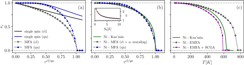
Figure 1: Benchmarks of magnetization curves using the mean field approximation (MFA) in the Heisenberg model. In panel (a), the MFA curves as function of the rescaled temperature $\tau^{\mathrm{cl/qu}}$ for classical (black dotted line) and quantum (blue dashed line) spins are compared to the single spin counterparts in a field $H_{\mathrm{eff}}^{0}$ (classical (black solid line) and quantum (blue solid line)). In panel (b), the classical (black dotted line) and quantum (blue dashed line) cases of the MFA for nickel are compared to the phenomenological Kuz’min curve (green solid line). The classical MFA is rescaled using the parameter $\alpha$ as found in the main text. The dependence of $\alpha$ on the spin length $S_{0}$ found in Eq. (4) is shown in the inset of panel (b). In panel (c), the MFA+environment (EMFA) (black dotted line) is compared to the EMFA with self–consistent Gaussian approximation (SCGA) (purple dashed line), and the Kuz’min curve (green solid line). Differently to the other panels, these magnetization curves are evaluated against the physical temperature, $T[K]$.

General setting.

We first consider the well–established Heisenberg model [26], which is described by the Hamiltonian $\mathcal{H}=-\sum_{\langle i,j\rangle}\frac{1}{2}J\hat{S}_{i}\hat{S}_{j}+\sum_{i}\gamma H_{\mathrm{ext}}\hat{S}_{i}^{z}$, where $J$ is the exchange parameter which can be calculated ab initio [27], $\gamma$ is the electron gyromagnetic ratio, $H_{\mathrm{ext}}$ is an external magnetic field pointing in the $z$ direction, the sum over $i$ runs over all the lattice sites, and $\langle i,j\rangle$ over nearest–neighbor pairs. For a system constituted by spins of length $S_{0}=n\hbar/2$ with $n=1,2,...$, the MFA self–consistent equation for the expectation value of the normalized spins  $s_{z}=\langle S_{z}\rangle/S_{0}$ is $s_{z}^{\mathrm{cl/qu}}=\mathcal{F}^{\mathrm{cl/qu}}\left(\beta\gamma H_{\mathrm{eff}}(s_{z})S_{0}\right)$ [29]. Here, $\beta=1/k_{B}T$ with $k_{B}$ the Boltzmann constant and $T$ the temperature, $\mathcal{F}^{\mathrm{cl/qu}}(x)$ is the Langevin function, $\mathcal{F}^{\mathrm{cl}}(x)=\coth(x)-1/x$, for the case of the classical Heisenberg model, and the Brillouin function, $\mathcal{F}^{\mathrm{qu}}(x)=\{(n+1)\coth\left[(n+1)x/n\right]-\coth\left(x/n\right)\}/n$, for the case of the quantum Heisenberg model [29]. Without loss of generality, the system is assumed to magnetize along the $z$ direction. Furthermore, $H_{\mathrm{eff}}(s_{z})=H_{\mathrm{ext}}+\mathsf{z}JS_{0}s_{z}/\gamma$ is the effective magnetic field felt by each spin in the lattice, with $\mathsf{z}$ being the coordination number.

It is quite insightful to express the magnetization curves $s_{z}^{\mathrm{cl/qu}}$ as a function of the relative temperatures $\tau^{\mathrm{cl/qu}}=T/T_{\mathrm{c}}^{\mathrm{cl/qu}}$. Here, $T_{\mathrm{c}}^{\mathrm{cl/qu}}$ are the critical temperatures marking the transition from the trivial solution $s_{z}^{\mathrm{cl/qu}}=0$ to the non–trivial solutions $s_{z}^{\mathrm{cl/qu}}\neq 0$. In the absence of an external magnetic field, $H_{\mathrm{ext}}=0$, the critical temperatures are $T_{\mathrm{c}}^{\mathrm{cl/qu}}=\mathsf{z}J\langle S^{2}\rangle^{\mathrm{cl/qu}}/(3k_{\mathrm{B}})$, where $\langle S^{2}\rangle^{\mathrm{cl}}=S_{0}^{2}$ for the classical case and $\langle S^{2}\rangle^{\mathrm{qu}}=S_{0}(S_{0}+\hbar)$ for the quantum one. These critical temperatures are typically overestimated since the MFA does not account for the system’s fluctuations [11]. Note that, in terms of the relative temperatures $\tau^{\mathrm{cl/qu}}$, the expectation value of the normalized spin takes the form

$$s_{z}^{\mathrm{cl/qu}}=\mathcal{F}^{\mathrm{cl/qu}}\left(\frac{3}{\tau^{\mathrm{cl/qu}}}\frac{S_{0}^{2}}{\langle S^{2}\rangle^{\mathrm{cl/qu}}}s_{z}^{\mathrm{cl/qu}}\right).$$ (1)

Therefore, the dependence of $s_{z}^{\mathrm{cl/qu}}$ in the Heisenberg model is reduced to just two free parameters, namely the relative temperature $\tau^{\mathrm{cl/qu}}$ and the spin length $S_{0}$.

The deviation of classical ASD simulations from experiments is most prominent at low temperatures [25], particularly so for magnetic materials with atoms carrying a small magnetic moment. Indeed, it is in this regime that quantum contributions play an important role in spin systems causing discrepancies between the classical and quantum results [30, 31, 32].

To see how these deviation originate, we can consider the spins at low temperature to be approximately in the ground state. The system then magnetizes along the $z$ direction, i.e. we can approximate on the right hand side of Eq. (1) $s_{z}\simeq 1$, thus resulting in the effective field independent of $s_{z}$, $H_{\mathrm{eff}}^{T=0}=\mathsf{z}JS_{0}/\gamma$. By means of the decoupling between spins and effective magnetic field, we can reduce the multi–spin physics to the study of a single spin in the constant effective magnetic field, $H_{\mathrm{eff}}^{T=0}$. This simple observation allows for a clear interpretation of the multi–spin physics at low temperatures. In fact, while a single classical spin has a continuous energy spectrum, the quantum counterpart does not. This implies that, already at the smallest finite temperature, the classical spin can experience infinitesimally excited states such that the expectation value $s_{z}$ deviates from the ground state $s_{z}=1$. On the other hand, the expectation value of the quantum spin remains in the ground state $s_{z}=1$ as long as the thermal energy $k_{\text{B}}T$ is smaller than the energy gap between the ground state and the first excited state, $\Delta E=\gamma H_{\mathrm{eff}}^{T=0}\hbar$.

In panel (a) of Fig. 1, we show the comparisons between the expectation value of a single spin in an effective field $H_{\mathrm{eff}}^{0}$ and the expectation value of a multi–spin system obtained from with the MFA as functions of the relative temperature $\tau^{\mathrm{cl/qu}}$. We do this for both the quantum and the classical case. In the limit of zero temperature, the single spin calculations (solid lines) closely resemble those obtained by means of the MFA (dotted and dashed lines). Note also that, while the classical spin (black lines) has a finite gradient at $T=0$, the quantum spin (blue line) is characterized by a plateau which only drops once $\tau^{\mathrm{qu}}\gtrsim 0.4$. That is, the classical spin is susceptible to arbitrarily small temperatures while, for the quantum case, there is a minimum amount of thermal energy needed to excite the system.

Power law temperature rescaling in the MFA.

The low temperature behavior of materials, being dominated by quantum effects, is often hard to capture in classical ASD simulations. In Ref. [25], Evans et. al. introduced a heuristic temperature rescaling to the ASD simulations to successfully reproduce the experimental temperature dependence of the magnetization. This temperature mapping from the classical to the quantum behavior was done by means of the rescaling

$$\tau^{\mathrm{cl}}=(\tau^{\mathrm{qu}})^{\alpha},$$ (2)

for a power $\alpha\in\mathds{R}$ that was fixed by fitting the simulations to experimental data. The same rescaling was also successful in matching the experimentally observed ultra–fast demagnetization in nickel [1].

Here, we provide a proof and a physical interpretation for the mechanism behind the success of such a rescaling. We further show that $\alpha$ depends exclusively on $S_{0}$, and give an analytical expression for $\alpha(S_{0})$. This can readily be used in ASD simulations to improve the low temperature descriptions at no additional computational cost.

To gain an understanding of the origin of this rescaling, we first note that the quantum–classical difference is already apparent in the MFA expression (1). We will thus fit the classical MFA solution, $s_{z}^{\mathrm{cl}}$, to the quantum one, $s_{z}^{\mathrm{qu}}$, assuming a temperature rescaling of the form of eq. (2). When expressing the temperature in terms of $\tau=T/T_{\mathrm{c}}$, the only free parameter left in the MFA is the spin length $S_{0}$ (see Eq. (1)). Therefore, to model the magnetization of a given material will require an appropriate choice of $S_{0}$. To do so, we write $S_{0}=n\hbar/2$ with $n=1,2,\dots$, and note that a spin of length $\hbar/2$ carries one Bohr magneton. We then choose the smallest integer $n$ that obeys $n\geq\mu[\mu_{\mathrm{B}}]$, where $\mu[\mu_{\mathrm{B}}]$ is the atomic magnetic moment of the material expressed in units of Bohr magnetons. These magnetic moments can be obtained e.g. by means of the augmented spherical wave (ASW) implementation of density functional theory [33]. Finally, we determine $\alpha$ in (2) by minimizing the mean squared error

$$\underset{\alpha}{\operatorname{argmin}}\int_{0}^{1}\mathrm{d}\tau\left[s_{z}^{\mathrm{qu}}(\tau)-s_{z}^{\mathrm{cl}}(\tau^{\alpha})\right]^{2},$$ (3)

where $s_{z}^{\mathrm{cl/qu}}$ are evaluated using (1).

To illustrate the results obtained with this procedure, we now look at the case of Ni, whose atomic magnetic moment is $\mu_{\mathrm{Ni}}=0.66\mu_{\mathrm{B}}$, which translates into a spin length $S_{0}=\hbar/2$. In Fig. 1 panel (b), we compare different magnetization curves for Ni, namely the quantum Heisenberg model $s_{z}^{\mathrm{qu}}(\tau^{\mathrm{qu}})$, the classical prediction with rescaled temperature $s_{z}^{\mathrm{cl}}((\tau^{\mathrm{qu}})^{\alpha})$, and the Kuz’min phenomenological model [34] which closely matches experiments. We observe great agreement between the quantum and classical rescaled magnetization curves, with a total global relative error of less than $2.5\%$ (see App. A, Fig. (2) for details). Moreover, we find that the classical magnetization curve with rescaled temperature is in great agreement with the phenomenological Kuz’min description, except for small deviations close to the critical temperature. It is worth noting that while we have focused on the example of Ni, the same procedure works successfully also for materials with other values of $S_{0}$, such as Gd (see App. B). We expect this to be the case as long as the material in question has a single coordination number $\mathsf{z}$ across the entire temperature range. In the inset of Fig. (1) panel (b), we plot the obtained scaling parameter $\alpha$ as a function of $S_{0}$ (black diamonds). We fit the obtained dependence $\alpha(S_{0})$ with the function

$$\alpha(S_{0})=1+\frac{2}{1+S_{0}/\hbar},$$ (4)

plotted in the same inset (red solid line). This extremely simple expression matches the results obtained from the numerical minimization with less than 0.05% error.

The obtained rescaling parameter as a function of $S_{0}$ is of great practical appeal, since it allows one to predict the observed experimental results via purely classical simulations. This is essential given that full quantum microscopic simulations of large systems are computationally unfeasible. Remarkably, our proven rescaling parameter $\alpha$, Eq. (4), perfectly matches the one used in Ref. [25] for nickel (we obtain $\alpha_{\rm Ni}=2.31$ whereas in Ref. [25] $\alpha_{\rm Ni}=2.32$ is reported). In Ref. [25], finding the parameter $\alpha$ required previously computing ASD simulation for a wide range of temperatures and fitting the results to experimental data. Here, instead, we determine $\alpha$ by matching the quantum and classical Heisenberg mean–field predictions. The benefits of this result are multiple. First, our approach does not require comparisons with experimental data, thus resulting in a self–contained solution. Second, it allows us to find the analytical expression in (4) which fully determines the values of $\alpha$ for a given material. Accounting for the rescaling (4) in ASD simulations then allows one to theoretically predict equilibrium magnetization and magnetization dynamics without previous reliance on experimental data. In conclusion, to account for quantum contributions at a given relative experimental temperature $\tau_{\mathrm{exp}}=T_{\mathrm{exp}}/T_{\mathrm{c}}$, one can use classical ASD simulations at a temperature $\tau_{\mathrm{sim}}=(\tau_{\mathrm{exp}})^{\alpha(S_{0})}$, where $\alpha(S_{0})$ is fully determined by (4) without impairing into any additional computational overhead.

Including environmental fluctuations.

The temperature rescaling strategy applied to relative temperatures $\tau$ relies on the prior knowledge of the experimental critical temperature $T_{\mathrm{c}}$ of the system. Here, we propose a strategy based on a modified ASD model accounting for environmental fluctuations, which can be fully parameterized by means of ab initio calculations. To show the predictive capabilities of such model we extend the MFA to the study systems coupled to an environment (EMFA). We furthermore correct our results with the self–consistent–Gaussian–approximation (SCGA) [35, 36]. The approach faithfully reproduces the absolute temperature dependence of the magnetization of several materials. As an example, we show the prediction of the magnetization curve for nickel and show that it can not only reproduce the low–temperature behavior to good accuracy, but also obtain an absolute critical temperature close to the experimental value.

In general, the study of magnetic materials needs to include the interaction between the atomic magnetic moments of the system (spins) with other, non–magnetic, degrees of freedom, such as phonons. To account for such degrees of freedom, we consider the spins in the Heisenberg model linearly coupled with independent baths of bosonic modes. This setting provides a microscopic model for the Landau–Lifshitz–Gilbert (LLG) equation as well as generalizations including inertial terms [37]. We assume isotropic coupling of the spins to these external modes and consider a Lorentzian spectral density for the baths. Note that the spectral density has a well–defined microscopic meaning and, in the case of phonons, is directly linked to the phonon density of state [38]. It is worth mentioning that the phonon density of state can be obtained with first principle calculations [39]. To perform our simulations on nickel, we parameterize the Lorentzian spectral density $J_{\omega}=(\eta/\pi)\omega_{0}^{4}\;\omega/((\omega^{2}-\omega_{0}^{2})^{2}+\omega^{2}\Gamma^{2})$ using the experimental phonon density of states reported in Ref. [40]. This sets a peak frequency at $\omega_{0}=6$ THz and its broadening at $\Gamma=8$ THz. The coupling strength is set by the dimension–free Gilbert damping $\eta$ [37], taken here as $\eta=0.01$, in line with values typically reported in the literature [41, 11].

The full quantum mechanical treatment of the Heisenberg model is unfeasible [42] and even more so in the case of an Heisenberg model interacting with a bosonic bath. To bypass this limitation, we assume classical spins interacting with a bath of harmonic oscillators with a quantum–like power spectrum [43, 19]. This is reminiscent of the techniques employed in Ref. [44] for the exact modeling of quantum Brownian motion via a semi–classical model. In Ref. [43], a semi–classical power spectrum $P_{\mathrm{sc}}\propto\coth\left(\frac{\hbar\omega}{2k_{B}T}\right)-1$ was used, in which the zero point fluctuations of the environment are removed. We here employ the same strategy.

While in principle the system described could be numerically solved for many spins, we here instead proceed to treat to problem via means of an extension of the MFA to systems interacting with an environment (EMFA). As we will see, this will be enough to allow us to make quantitative predictions of the magnetization as a function of temperature in real units and to reproduce the low–temperature behavior of the many–spin system. To do so, we write the self–consistent mean field equation

$$\bm{S}=\mathcal{\bm{F}}_{\mathrm{EMF}}(\bm{H}_{\mathrm{eff}}[\bm{S}])=\frac{\text{Tr}[\bm{S}e^{-\beta(H_{\mathrm{B}}-\bm{H}_{\mathrm{eff}}[\bm{S}]\cdot\bm{S})}]}{\text{Tr}[e^{-\beta(H_{\mathrm{B}}-\bm{H}_{\mathrm{eff}}[\bm{S}]\cdot\bm{S})}]},$$ (5)

where $\bm{S}$ is the spin vector and $\mathcal{F}_{\mathrm{EMF}}$ is the functional form of the thermal expectation value of a spin in an effective magnetic field $\bm{H}_{\mathrm{eff}}[\bm{S}]=\mathsf{z}J\bm{S}/\gamma+\int_{0}^{\infty}d\omega\sqrt{2\omega J_{\omega}}\bm{X}_{\omega}$  [32]. Here, $H_{\mathrm{B}}=\int_{0}^{\infty}\mathrm{d}\omega(\bm{P}_{\omega}^{2}+\omega^{2}\bm{X}_{\omega}^{2})/2$ is the Hamiltonian of the environmental bosonic modes, with $\bm{X}_{\omega}$ and $\bm{P}_{\omega}$ their respective positions and momenta, and $\text{Tr}[\circ]$ is the integral over all the dynamical variables. To evaluate $\mathcal{F}_{\mathrm{EMF}}$ on the right–hand–side of Eq. (5), for each value of $\beta$ we solve the classical spin dynamics to find the dynamical steady–state in the presence of the field $H_{\mathrm{eff}}$ and in contact with the semi–classical environment using the numerical method described in Ref. [37, 45]. Finally, we numerically solve the self–consistent equation (5) to find the equilibrium spin expectation value $s_{z}(T)$. The main limitation of the mean field methods is the inability to properly account for fluctuations. Therefore, to improve the accuracy of our method, we further introduce corrections by means of the SCGA [36, 35].

In Fig. (1) panel (c), the purple dashed line shows the temperature dependence of the magnetization for nickel as predicted by our approach (EMFA+SCGA). Note that here we plot against the physical temperature (evaluated in Kelvin, $T[\mathrm{K}]$) and not the relative temperature ($\tau^{\mathrm{cl/qu}}$). The (EMFA+SCGA) approach is compared with the results of the EMFA (black dotted line) and with the phenomenological Kuz’min [34] curve (green solid line) which is known to reproduce the experimental behavior. As shown in the figure, both EMFA and EMFA+SCGA give a good prediction of the experimental $s_{z}(T)$ trend as a function of the absolute temperature in K. The EMFA gives a prediction for the critical temperature of $T_{\mathrm{c}}^{\mathrm{EMFA}}=745\,\mathrm{K}$ while the EMFA+SCGA provides $T_{\mathrm{c}}^{\mathrm{EMFA+SCGA}}=590\,\mathrm{K}$ which is in good agreement with the experimental critical temperature $T_{\mathrm{c}}^{\mathrm{exp}}=632\,\mathrm{K}$. Note that, the accuracy in the low–temperature prediction is a direct consequence of the introduction of the environment. Indeed, in the absence of the environment, the EMFA reduces to the standard MFA, and both classical MFA and MFA+SCGA (without environment nor temperature rescaling) fail to capture the qualitative behavior in this regime (see also App. C for details).

The magnetization curves produced by our approach (see Fig. (1) panel (c)) prove to be in extremely good agreement with the experimental results for nickel in the whole temperature range $T=[0,T_{\mathrm{c}}]$. In particular, it accurately reproduces the magnetization behavior at low temperature, which standard atomistic spin dynamics techniques struggle to describe [25].

Thus, by implementing the coupled equations of motion derived from this semi–classical Heisenberg model interacting with a parameterized environment, one obtains a magnetization dynamics based on ab initio evaluations. This approach, in addition to account for quantum effects, would result in tractable equations of motion for the current computational resources.

Summary and conclusions.

In this letter we present a set of tools aimed to account for quantum corrections in ASD. Firstly, we showed that, introducing a power–law temperature rescaling, the classical MFA can accurately reproduce the temperature dependence of the quantum MFA magnetization. This power–law rescaling takes the form $\tau^{\mathrm{cl}}=(\tau^{\mathrm{qu}})^{\alpha(S_{0})}$ where $\alpha(S_{0})$ is an intrinsic property of the system and depends only on the spin length $S_{0}$. The rescaling parameters $\alpha(S_{0})$ obtained for Ni appears to be in very good agreement with the values of Ref. [25], used to reproduce experimental results via dynamical ASD simulations. However, in our case, $\alpha(S_{0})$ does not require a priori knowledge of the microscopic description of the system nor previously fitting demanding simulations to experimental results. Despite its simplicity, our approach can be easily combined with ASD to account for quantum effects. This result gives a clear prescription on how to account for quantum effects in ASD simulations. To do this, it is sufficient to calculate the rescaling parameter $\alpha(S_{0})$ by using Eq. (4) and run ASD simulations at a temperature $\tau_{{\rm sim}}=\tau_{{\rm exp}}^{\alpha(S_{0})}$.

Second, we extended the MFA to the study of a semi–classical open Heisenberg model in contact with environmental degrees of freedom such as, for examples, phonons. The parameters of the model can be directly calculated by means of ab initio calculations or extracted from experiments. We further introduced corrections to the MFA of the semi–classical open Heisenberg model by means of the SCGA. We found very good agreement between the magnetization curves of nickel predicted by this method and the experimental results, particularly for low temperatures. The predicted magnetization is furthermore capable of reproducing the absolute experimental $T_{\mathrm{c}}$ to good accuracy. This suggests that the semi–classical model considered can be used to faithfully predict the dynamics of magnetic materials at all temperatures.

Our results are a substantial step forward towards effectively including quantum aspects of the spin dynamics in magnetic calculations. When implemented in a large scale ASD framework, we believe they would provide a more accurate description of the magnetisation dynamics at low temperatures.

Appendix A A. Error of the MF temperature–rescaling

Here we show the error of the temperature rescaling shown in Fig.1 panel (b). We use as error measure the relative root mean square error (RRMSE), defined as

$$\mathrm{RRMSE}=\sqrt{\frac{\int_{0}^{1}\mathrm{d}\tau\left[s_{z}^{\mathrm{qu}}(\tau)-s_{z}^{\mathrm{cl}}(\tau^{\alpha})\right]^{2}}{\int_{0}^{1}\mathrm{d}\tau\left[s_{z}^{\mathrm{qu}}(\tau)\right]^{2}}}.$$ (6)

In Fig.2 we plot the RRMSE in percentage as a function of the spin length $S_{0}$. In the worst–case, the error is at most 2.5%, and it decreases as $S_{0}$ increases, as expected from the fact that as $S_{0}$ increases the quantum magnetization curve converges to the classical one.

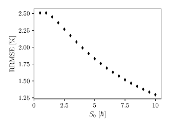
Figure 2: Error of the MF temperature rescaling. Plot of the RRMSE as defined in (6) as a function of spin length $S_{0}$.

Appendix B B. Results for Gd

In Fig. 3, we show the analogous plot of Fig. 1 panel (b) for the case of gadolinium, which has an effecitve $S_{0}=4$. We compare the quantum MFA magnetization curve, the rescaled classical MFA magnetization curve using the calculated $\alpha=1.4$ (which compares well with the value of $\alpha=1.28$ reported in [25]) and the Kuz’min curve (green line).

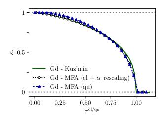
Figure 3: Mean-field temperature rescaling for Gd. Analogous to Fig.1 panel (b) but for the case of Gd.

Appendix C C. Comparison of MFA vs EMFA

In the absence of the environment, the EMFA reduces to the standard MFA of the Heisenberg model. At low temperatures the MFA (without any temperature rescaling) is unable to properly describe the low temperature behavior of the magnetization. This is illustrated in Fig.4 where we plot the MFA and the EMFA in terms of the relative temperature $\tau=T/T_{\mathrm{c}}$. Indeed, we see that the EMFA, by including the effects of the environment, is able to significantly better describe the magnetization across the whole temperature range.

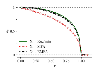
Figure 4: Comparison of MFA vs EMFA for Ni. Plot of the MFA of the classical Heisenberg model (red diamonds) and the semi–classical EMFA model (black diamonds) as a function of the relative temperature $T/T_{\mathrm{c}}$. We further plot the Kuz’min phenomenological fit of the experimentally measured magnetisation of Ni.