Exact Generalization Guarantees for (Regularized) Wasserstein Distributionally Robust Models

Abstract

Wasserstein distributionally robust estimators have emerged as powerful models for prediction and decision-making under uncertainty. These estimators provide attractive generalization guarantees: the robust objective obtained from the training distribution is an exact upper bound on the true risk with high probability. However, existing guarantees either suffer from the curse of dimensionality, are restricted to specific settings, or lead to spurious error terms. In this paper, we show that these generalization guarantees actually hold on general classes of models, do not suffer from the curse of dimensionality, and can even cover distribution shifts at testing. We also prove that these results carry over to the newly-introduced regularized versions of Wasserstein distributionally robust problems.

1 Introduction

1.1 Generalization and (Wasserstein) Distributionally Robust Models

We consider the fundamental question of generalization of machine learning models. Let us denote by ${f}_{\theta}$ the loss induced by a model parametrized by ${\theta}$ for some uncertain variable ${\xi}$ (typically a data point). When ${\xi}$ follows some distribution $\operatorname{P}$, seeking the best parameter ${\theta}$ writes as minimizing the expected loss

$$\min_{{\theta}\in{\Theta}}~{}\mathbb{E}_{{\xi}\sim\operatorname{P}}\left[{f}_{\theta}({\xi})\right]\,.$$ (1)

We usually do not have a direct knowledge of $\operatorname{P}$ but rather we have access to samples $({\xi}_{i})_{{i}=1}^{n}$ independently drawn from $\operatorname{P}$. The empirical risk minimization approach then consists in minimizing the expected loss over the associated empirical distribution $\operatorname{\WAedit{\widehat{\operatorname{P}}_{{n}}}}={\frac{1}{{n}}\sum_{{i}=1}^{n}}\delta_{{\xi}_{i}}$ (as a proxy for the expected loss over $\operatorname{P}$), i.e.,

$$\min_{{\theta}\in{\Theta}}~{}\mathbb{E}_{{\xi}\sim\operatorname{\WAedit{\widehat{\operatorname{P}}_{{n}}}}}\left[{f}_{\theta}({\xi})\right]~{}\left(=\frac{1}{{n}}\sum_{{i}=1}^{n}{f}_{\theta}({\xi}_{i})\right).$$ (2)

Classical statistical learning theory ensures that, with high probability, $\mathbb{E}_{\operatorname{P}}\left[{{f}}_{\theta}\right]$ is close to $\mathbb{E}_{\operatorname{\WAedit{\widehat{\operatorname{P}}_{{n}}}}}\left[{{f}}_{\theta}\right]$ up to $\operatorname{\mathcal{O}}\left({1}/{\sqrt{n}}\right)$ error terms, see e.g., the monographs Boucheron et al. (2013); Wainwright (2019).

A practical drawback of empirical risk minimization is that it can lead to over-confident decisions (when $\mathbb{E}_{\operatorname{\WAedit{\widehat{\operatorname{P}}_{{n}}}}}\left[{{f}}_{\theta}\right]<\mathbb{E}_{\operatorname{P}}\left[{{f}}_{\theta}\right]$, the real loss can be higher that the empirical one (Esfahani and Kuhn, 2018)). In addition, this approach is also sensitive to distribution shifts between training and application. To overcome these drawbacks, an approach gaining momentum in machine learning is distributionally robust optimization, which consists in minimizing the worst expectation of the loss when the distribution lives in a neighborhood of $\operatorname{\WAedit{\widehat{\operatorname{P}}_{{n}}}}$:

$$\min_{{\theta}\in{\Theta}}~{}\sup_{\operatorname{Q}\in{{\mathcal{U}}}(\operatorname{\WAedit{\widehat{\operatorname{P}}_{{n}}}})}\mathbb{E}_{{\xi}\sim\operatorname{Q}}\left[{f}_{\theta}({\xi})\right]\,,$$ (3)

where the inner $\sup$ is thus taken over $\operatorname{Q}$ in the neighborhood ${{\mathcal{U}}}(\operatorname{\WAedit{\widehat{\operatorname{P}}_{{n}}}})$ of $\operatorname{\WAedit{\widehat{\operatorname{P}}_{{n}}}}$ in the space of probability distributions. Popular choices of distribution neighborhoods are based on the Kullback-Leibler (KL) divergence (Laguel et al., 2020; Levy et al., 2020), kernel tools (Zhu et al., 2021a; Staib and Jegelka, 2019; Zhu et al., 2021b), moments (Delage and Ye, 2010; Goh and Sim, 2010), or Wasserstein distance (Shafieezadeh Abadeh et al., 2015; Esfahani and Kuhn, 2018). If $\operatorname{P}\in{{\mathcal{U}}}(\operatorname{\WAedit{\widehat{\operatorname{P}}_{{n}}}})$, distributionally robust models can benefit from direct generalization guarantees as,

$$\sup_{\operatorname{Q}\in{{\mathcal{U}}}(\operatorname{\WAedit{\widehat{\operatorname{P}}_{{n}}}})}\mathbb{E}_{{\xi}\sim\operatorname{Q}}\left[{f}_{\theta}({\xi})\right]~{}~{}\geq~{}~{}\mathbb{E}_{{\xi}\sim\operatorname{P}}\left[{f}_{\theta}({\xi})\right].$$ (4)

Thus, for well-chosen neighborhoods ${{\mathcal{U}}}(\operatorname{\WAedit{\widehat{\operatorname{P}}_{{n}}}})$, distributionally robust objectives are able to provide exact upper-bounds on the expected loss over distribution $\operatorname{P}$, i.e., the true risk.

Wasserstein distributionally robust optimization (WDRO) problems correspond to (3) with

$${{\mathcal{U}}}(\operatorname{\WAedit{\widehat{\operatorname{P}}_{{n}}}})=\left\{\operatorname{Q}\in\mathcal{P}({\Xi}):W(\operatorname{\WAedit{\widehat{\operatorname{P}}_{{n}}}},\operatorname{Q})\leq{\rho}\right\}\,,$$ (5)

where $W(\operatorname{\WAedit{\widehat{\operatorname{P}}_{{n}}}},\operatorname{Q})$ denotes the Wasserstein distance between $\operatorname{\WAedit{\widehat{\operatorname{P}}_{{n}}}}$ and $\operatorname{Q}$ and ${\rho}>0$ controls the required level of robustness around $\operatorname{\WAedit{\widehat{\operatorname{P}}_{{n}}}}$. As a natural metric to compare discrete and absolutely continuous probability distributions, the Wasserstein distance has attracted a lot of interest in both machine learning (Shafieezadeh Abadeh et al., 2015; Sinha et al., 2018; Shafieezadeh-Abadeh et al., 2019; Li et al., 2020; Kwon et al., 2020) and operation research (Zhao and Guan, 2018; Arrigo et al., 2022) communities; see e.g., the review articles Blanchet et al. (2021); Kuhn et al. (2019).

WDRO benefits from out-of-the-box generalization guarantees in the form of (4) since it inherits the concentration properties of the Wasserstein distance (Esfahani and Kuhn, 2018). More precisely, under mild assumptions on $\operatorname{P}$, (Fournier and Guillin, 2015) establishes that $W(\operatorname{\WAedit{\widehat{\operatorname{P}}_{{n}}}},\operatorname{P})\leq{\rho}$ with high probability as soon as ${\rho}\sim 1/{n}^{1/{{d}}}$ where ${{d}}$ denotes the dimension of the samples space. Thus, a major issue is the prescribed radius ${\rho}$ suffers from the curse of the dimensionality: when ${{d}}$ is large, ${\rho}$ decreases slowly as the number of samples ${n}$ increases. This constrasts with other distributionally robust optimization ambiguity sets, such as Maximum Mean Discrepancy (MMD) (Staib and Jegelka, 2019; Zeng and Lam, 2022), where the radius scales as $1/\sqrt{n}$. Moreover, the existing scaling for WDRO is overly conservative for WDRO objectives since recent works (Blanchet et al., 2022a; Blanchet and Shapiro, 2023) prove that a radius behaving as $1/\sqrt{n}$ is asymptotically optimal. The main difference with (Esfahani and Kuhn, 2018) is that they — and us — consider the WDRO objective as a whole, instead of proceeding in two steps: first considering the Wasserstein distance independently and invoking concentration results on the Wasserstein distance and then plugging this result in the WDRO problem.

1.2 Contributions and related works

In this paper, we show that WDRO provides exact upper-bounds on the true risk with high probability. More precisely, we prove non-asymptotic generalization bounds of the form of Eq. 4, that hold for general classes of functions, and that only require ${\rho}$ to scale as $1/\sqrt{n}$ and not $1/{n}^{1/{{d}}}$. To do so, we construct an interval for the radius ${\rho}$ for which it is both sufficiently large so that we can go from the empirical to the true estimator (i.e., at least of the order of $1/\sqrt{n}$) and sufficiently small so that the robust problem does not become degenerate (i.e., smaller than some critical radius, that we introduce as an explicit constant). Our results imply proving concentration results on Wasserstein Distributionally Robust objectives that are of independent interest.

This work is part of a rich and recent line of research about theoretical guarantees on WDRO for machine learning. One of this first results, Lee and Raginsky (2018), provides generalization guarantees, for a general class of models and a fixed ${\rho}$, that, however, become degenerate as the radius goes to zero. In the particular case of linear models, WDRO models admit an explicit form that allows Shafieezadeh-Abadeh et al. (2019); Chen and Paschalidis (2018) to provide generalization guarantees Eq. 4 with the radius scaling as $1/\sqrt{n}$. The case of general classes of models, possibly non-linear, is more intricate. Sinha et al. (2018) showed that a modified version of Eq. 4 holds at the price of non-negligible error terms. Gao (2022); An and Gao (2021) made another step towards broad generalization guarantees for WDRO but with error terms that vanish only when ${\rho}$ goes to zero.

In contrast, our analysis provides exact generalization guarantees in the form Eq. 4 without additional error terms, that hold for general classes of functions and allow for a non-vanishing uncertainty radius to cover for distribution shifts at testing. Moreover, our guarantees also carry over to the recently introduced regularized versions of WDRO (Wang et al., 2023; Azizian et al., 2023), whose statistical properties have not been studied yet.

This paper is organized as follows. In Section 2, we introduce notations and our blanket assumptions. In Section 3, we present our main results, an idea of proof, and discussions. The complete proofs are deferred to the appendix.

2 Setup and Assumptions

In this section, we formalize our setting and introduce Wasserstein Distributionally Robust risks.

2.1 Wasserstein Distributionally Robust risk functions

In this paper, we consider as a samples space ${\Xi}$ a subset of $\mathbb{R}^{{d}}$ equipped with the Euclidean norm $\lVert\cdot\rVert$. We rely on Wasserstein distances of order $2$, in line with the seminal work Blanchet et al. (2022a) on generalization of WDRO. This distance is defined for two distributions $\operatorname{Q},\operatorname{Q}^{\prime}$ in the set of probability distributions on ${\Xi}$, denoted by $\mathcal{P}({\Xi})$, as

$$W_{2}(\operatorname{Q},\operatorname{Q}^{\prime})\coloneqq\left(\inf_{\operatorname{\pi}\in\mathcal{P}({\Xi}\times{\Xi}),\operatorname{\pi}_{1}=\operatorname{Q},\operatorname{\pi}_{2}=\operatorname{Q}^{\prime}}\mathbb{E}_{({\xi},{{\zeta}})\sim\operatorname{\pi}}\left[\frac{1}{2}\|{\xi}-{{\zeta}}\|^{2}\right]\right)^{1/2}\,,$$ (6)

where $\mathcal{P}({\Xi}\times{\Xi})$ is the set of probability distributions in the product space ${\Xi}\times{\Xi}$, and $\operatorname{\pi}_{1}$ (resp. $\operatorname{\pi}_{2}$) denotes the first (resp. second) marginal of $\operatorname{\pi}$.

We denote by ${f}:{\Xi}\to\mathbb{R}$ the loss function of some model over the sample space. The model may depend on some parameter ${\theta}$, that we drop for now to lighten the notations; instead, we consider a class of functions ${\mathcal{F}}$ encompassing our various models and losses of interest (we come back to classes of parametric models of the form ${\mathcal{F}}=\{{f}_{\theta}:{\theta}\in{\Theta}\}$ in Section 4).

We define the empirical Wasserstein Distributionally Robust risk $\widehat{\mathcal{R}}_{{\rho}^{2}}({f})$ centered on $\operatorname{\WAedit{\widehat{\operatorname{P}}_{{n}}}}$ and similarly the true robust risk ${\mathcal{R}}_{{\rho}^{2}}({f})$ centered on $\operatorname{P}$ as

$$\widehat{\mathcal{R}}_{{\rho}^{2}}({f})\coloneqq\sup_{\begin{subarray}{c}\operatorname{Q}\in\mathcal{P}({\Xi})\\ W^{2}_{2}(\operatorname{\WAedit{\widehat{\operatorname{P}}_{{n}}}},\operatorname{Q})\leq{\rho}^{2}\end{subarray}}\mathbb{E}_{{\xi}\sim\operatorname{Q}}\left[{f}({\xi})\right]\qquad\text{and}\qquad{\mathcal{R}}_{{\rho}^{2}}({f})\coloneqq\sup_{\begin{subarray}{c}\operatorname{Q}\in\mathcal{P}({\Xi})\\ W^{2}_{2}(\operatorname{P},\operatorname{Q})\leq{\rho}^{2}\end{subarray}}\mathbb{E}_{{\xi}\sim\operatorname{Q}}\left[{f}({\xi})\right]\,.$$ (7)

Note that $\widehat{\mathcal{R}}_{{\rho}^{2}}({f})$, which is based on the empirical distribution $\operatorname{\WAedit{\widehat{\operatorname{P}}_{{n}}}}$, is a computable proxy for the true robust risk ${\mathcal{R}}_{{\rho}^{2}}({f})$. Note also that the true robust risk ${\mathcal{R}}_{{\rho}^{2}}({f})$ immediately upper-bounds the true (non-robust) risk $\mathbb{E}_{{\xi}\sim\operatorname{P}}\left[{f}({\xi})\right]$ and also upper-bounds $\mathbb{E}_{{\xi}\sim\operatorname{Q}}\left[{f}({\xi})\right]$ for neighboring distributions $\operatorname{Q}$ that correspond to distributions shifts of magnitude smaller than ${\rho}$ in Wasserstein distance.

2.2 Regularized versions

Entropic regularization of WDRO problems was recently studied in Wang et al. (2023); Blanchet and Kang (2020); Piat et al. (2022); Azizian et al. (2023) and used in Dapogny et al. (2023); Song et al. (2023); Wang and Xie (2022); Wang et al. (2022). Inspired by the entropic regularization in optimal transport (OT) (Peyré and Cuturi, 2019, Chap. 4), the idea is to regularize the objective by adding a KL divergence, that is defined, for any transport plan $\operatorname{\pi}\in\mathcal{P}({\Xi}\times{\Xi})$ and a fixed reference $\overline{\operatorname{\pi}}\in\mathcal{P}({\Xi}\times{\Xi})$, by

$$\operatorname{KL}(\operatorname{\pi}|\overline{\operatorname{\pi}})=\begin{cases}\int\log\frac{{\mathrm{d}}\operatorname{\pi}}{{\mathrm{d}}\overline{\operatorname{\pi}}}\,{\mathrm{d}}\operatorname{\pi}&\text{when}\operatorname{\pi}\ll\overline{\operatorname{\pi}}\\ +\infty&\text{otherwise}.\end{cases}$$ (8)

Unlike in OT though, the choice of the reference measure in WDRO is not neutral and introduces a bias in the robust objective (Azizian et al., 2023). For their theoretical convenience, we take reference measures that have Gaussian conditional distributions

$$\operatorname{\pi}_{\sigma}({\mathrm{d}}{{\zeta}}|{\xi})\propto\operatorname{\mathds{1}}_{{\zeta}\in{\Xi}}e^{-\frac{\lVert{\xi}-{\zeta}\rVert^{2}}{2{\sigma}^{2}}}{\mathrm{d}}{{\zeta}},\qquad\text{for all }{\xi}\in{\Xi}\,,$$ (9)

where ${\sigma}>0$ controls the spread of the second marginals, following Wang et al. (2023); Azizian et al. (2023). Then, the regularized version of $\widehat{\mathcal{R}}_{{\rho}^{2}}({f})$ (WDRO empirical risk) is given by

$$\widehat{\mathcal{R}}^{{\varepsilon}}_{{\rho}^{2}}({f}) \coloneqq\sup_{\begin{subarray}{c}\operatorname{\pi}\in\mathcal{P}({\Xi}\times{\Xi}),\operatorname{\pi}_{1}=\operatorname{\WAedit{\widehat{\operatorname{P}}_{{n}}}}\\ \mathbb{E}_{({\xi},{{\zeta}})\sim\operatorname{\pi}}\left[\frac{1}{2}\|{\xi}-{{\zeta}}\|^{2}\right]\leq{\rho}^{2}\end{subarray}}\mathbb{E}_{{\xi}\sim\operatorname{\pi}_{2}}\left[{f}({\xi})\right]-{\varepsilon}\operatorname{KL}\left(\operatorname{\pi}\left|\operatorname{\pi}^{n}_{\sigma}\right.\right)\qquad\text{with }\operatorname{\pi}^{n}_{\sigma}=\operatorname{\WAedit{\widehat{\operatorname{P}}_{{n}}}}({\mathrm{d}}{\xi})\operatorname{\pi}_{\sigma}({\mathrm{d}}{{\zeta}}|{\xi})$$ (10)

and similarly, the regularized version of ${\mathcal{R}}_{{\rho}^{2}}({f})$ is given by

$${\mathcal{R}}^{{\varepsilon}}_{{\rho}^{2}}({f}) \coloneqq\sup_{\begin{subarray}{c}\operatorname{\pi}\in\mathcal{P}({\Xi}\times{\Xi}),\operatorname{\pi}_{1}=\operatorname{P}\\ \mathbb{E}_{({\xi},{{\zeta}})\sim\operatorname{\pi}}\left[\frac{1}{2}\|{\xi}-{{\zeta}}\|^{2}\right]\leq{\rho}^{2}\end{subarray}}\mathbb{E}_{{\xi}\sim\operatorname{\pi}_{2}}\left[{f}({\xi})\right]-{\varepsilon}\operatorname{KL}\left(\operatorname{\pi}\left|\operatorname{\pi}_{\sigma}\right.\right)\qquad\text{with }\operatorname{\pi}_{\sigma}=\operatorname{P}({\mathrm{d}}{\xi})\operatorname{\pi}_{\sigma}({\mathrm{d}}{{\zeta}}|{\xi}).$$ (11)

These regularized risks have been studied in terms of computational or approximation properties, but their statistical properties have not been investigated yet. The analysis we develop for WDRO estimators is general enough to carry over to these settings.

In Eqs. 10 and 11, note finally that the regularization is added as a penalization in the supremum, rather than in the constraint. As in Wang et al. (2023), penalizing in the constraint leads to an ambiguity set defined by the regularized Wasserstein distance, that we introduce in Section 3.2. We refer to Azizian et al. (2023) for a unified presentation of the two penalizations.

2.3 Blanket assumptions

Our analysis is carried under the following set of assumptions that will be in place throughout the paper. First, we assume that the sample space ${\Xi}\subset\mathbb{R}^{{d}}$ is convex and compact, which is in line with previous work, e.g., (Lee and Raginsky, 2018; An and Gao, 2021).

Assumption 1 (On the set ${\Xi}$).

The sample space ${\Xi}$ is a compact convex subset of $\mathbb{R}^{{d}}$.

Second, we require the class of loss functions ${\mathcal{F}}$ to be sufficiently regular. In particular, we assume that they have Lipschitz continuous gradients.

Assumption 2 (On the function class).

The functions of ${\mathcal{F}}$ are twice differentiable, uniformly bounded, and their derivatives are uniformly bounded and uniformly Lipschitz.

Finally, we assume that $\operatorname{\WAedit{\widehat{\operatorname{P}}_{{n}}}}$ is made of independent and identically distributed (i.i.d.) samples of $\operatorname{P}$ and that $\operatorname{P}$ is supported on the interior of ${\Xi}$ (which can be done without loss of generality by slightly enlarging ${\Xi}$ if needed).

Assumption 3 (On the distributions).

$\operatorname{\WAedit{\widehat{\operatorname{P}}_{{n}}}}=\frac{1}{{n}}\sum_{i=1}^{n}\delta_{{\xi}_{i}}$ where ${\xi}_{1},\dots,{\xi}_{n}$ are i.i.d. samples of $\operatorname{P}$. We further assume that there is some ${R}>0$ such that $\operatorname{P}$ satisfies $\operatorname{supp}\operatorname{P}+{\overline{\mathbb{B}}}(0,{R})\subset{\Xi}$.

3 Main results and discussions

The main results of our paper establish that the empirical robust risk provide high probability bounds, of the form of Eq. 4, on the true risk. Since the results and assumptions slightly differ between the WDRO models and their regularized counterparts, we present them separately in Section 3.1 and Section 3.2. In Section 3.3, we provide the common outline for the proofs of these results, the proofs themselves being provided in the appendix. Finally, in Section 4, we detail some examples.

3.1 Exact generalization guarantees for WDRO models

In this section, we require the two following additional assumptions on the function class. The first assumption is common in the WDRO litterature, see e.g., Blanchet et al. (2022a); Blanchet and Shapiro (2023); Gao (2022); An and Gao (2021).

Assumption 4.

The quantity $\inf_{{{f}}\in{\mathcal{F}}}\mathbb{E}_{\operatorname{P}}\left[\lVert\operatorname{\nabla}{{f}}\rVert^{2}\right]$ is positive.

The second assumption we consider in this section makes use of the notation ${d}({\xi},A)$, for a set $A\subset{\Xi}$ and a point ${\xi}\in{\Xi}$, to denote the distance between ${\xi}$ and $A$, i.e., ${d}({\xi},A)=\inf_{{{\zeta}}\in A}\lVert{\xi}-{{\zeta}}\rVert$.

Assumption 5.

1. For any ${R}>0$, there exists ${\Delta}>0$ such that,

   $$\forall{{f}}\in{\mathcal{F}},\,\forall{{\zeta}}\in{\Xi},\quad{d}({{\zeta}},\operatorname*{arg\,max}{{f}})\geq{R}\implies{{f}}({{\zeta}})-\max{{f}}\leq-{\Delta}\,.$$ (12)

2. The following growth condition holds: there exist ${\mu}>0$ and ${L}>0$ such that, for all ${{f}}\in{\mathcal{F}}$, ${\xi}\in{\Xi}$ and ${\xi^{*}}$ a projection of ${\xi}$ on $\operatorname*{arg\,max}{{f}}$, i.e., ${\xi^{*}}\in\operatorname*{arg\,min}_{\operatorname*{arg\,max}{{f}}}\lVert{\xi}-\cdot\rVert$,

   $${{f}}({\xi^{*}})\geq{{f}}({\xi})+\frac{{\mu}}{2}\lVert{\xi}-{\xi^{*}}\rVert^{2}-\frac{{L}}{6}\lVert{\xi}-{\xi^{*}}\rVert^{3}\,.$$ (13)

The first item of this assumption has a natural interpretation: we show in Section A.4, that it is equivalent to the relative compactness of the function space ${\mathcal{F}}$ w.r.t. to the distance

$${D}({{f}},{{g}})\coloneqq\lVert{{f}}-{{g}}\rVert_{\infty}+{D_{H}}(\operatorname*{arg\,max}{{f}},\operatorname*{arg\,max}{{g}})\,,$$ (14)

where ${D_{H}}$ denotes the (Hausdorff) distance between sets and $\lVert{{f}}\rVert_{\infty}\coloneqq\sup_{{\xi}\in{\Xi}}\lvert{{f}}({\xi})\rvert$ is the infinity norm. The last one is a structural assumption on the functions ${\mathcal{F}}$ that is new in our context but is actually very close the so-called parametric Morse-Bott condition, introduced in of bilevel optimization (Arbel and Mairal, 2022), see Section A.5.

We now state our main generalization result for WDRO risks.

Theorem 3.0.

Under Assumptions 4 and 5, there is an explicit constant ${\rho}_{c}$ depending only on ${\mathcal{F}}$ and $\operatorname{P}$ such that for any ${\delta}\in(0,1)$ and ${n}\geq 1$, if

$$\operatorname{\mathcal{O}}\left(\sqrt{\frac{1+{\log 1/{\delta}}}{{n}}}\right)\leq{\rho}\leq\frac{{\rho}_{c}}{2}-\operatorname{\mathcal{O}}\left(\sqrt{\frac{1+\log 1/{\delta}}{{n}}}\right)$$ (15)

then, there is ${\rho}_{n}=\operatorname{\mathcal{O}}\left(\sqrt{\frac{1+{\log 1/{\delta}}}{{n}}}\right)$ such that, with probability $1-{\delta}$,

$$\forall{f}\in{\mathcal{F}},\quad\widehat{\mathcal{R}}_{{\rho}^{2}}({f})\geq\mathbb{E}_{{\xi}\sim\operatorname{Q}}\left[{f}({\xi})\right]\qquad\text{for all }\operatorname{Q}\text{such that $W^{2}_{2}(\operatorname{P},\operatorname{Q})\leq{\rho}({\rho}-{\rho}_{n})$}\,.$$ (16)

In particular, with probability $1-{\delta}$, we have

$$\forall{f}\in{\mathcal{F}},\quad\widehat{\mathcal{R}}_{{\rho}^{2}}({f})\geq\mathbb{E}_{{\xi}\sim\operatorname{P}}\left[{f}({\xi})\right].$$ (17)

The second part of the result, Eq. 17, is an exact generalization bound: it is an actual upper-bound on the true risk $\mathbb{E}_{{\xi}\sim\operatorname{P}}\left[{{f}}({\xi})\right]$, that we cannot access in general, through a quantity that we can actually compute with $\operatorname{\WAedit{\widehat{\operatorname{P}}_{{n}}}}$. The first part of the result, Eq. 16 gives us insight into the robustness guarantees offered by the WDRO risk. Indeed, it tells us that, when ${\rho}$ is greater than the minimal radius ${\rho}_{n}\propto 1/\sqrt{n}$ by some margin, the empirical robust risk $\widehat{\mathcal{R}}_{{\rho}^{2}}({f})$ is an upper-bound on the loss even with some perturbations of the true distribution. Hence, as long as ${\rho}$ is large enough, the WDRO objective enables us to guarantee the performance of our model even in the event of a distribution shift at testing time. In other words, the empirical robust risk is an exact upper-bound on the true robust risk ${\mathcal{R}}_{{\rho}({\rho}-{\rho}_{n})}({f})$ with a reduced radius.

The range of admissible radiuses is described by Eq. 15. The lower-bound, roughly proportional to $1/\sqrt{n}$, is optimal, following the results of Blanchet et al. (2022a). The upper-bound, almost independent of ${n}$, depends on a constant ${\rho}_{c}$, that we call critical radius and that has an interesting interpretation, that we formalize in the following remark. Note, finally, that, the big-O notation in this theorem has a slightly stronger meaning than the usual one, being non-asymptotic in ${n}$ and ${\delta}$.

Remark 3.0 (Interpretation of critical radius).

The critical radius ${\rho}_{c}$, appearing in Eq. 15, is defined by

$${\rho}_{c}^{2}\coloneqq\inf_{{{f}}\in{\mathcal{F}}}\mathbb{E}_{{\xi}\sim\operatorname{P}}\left[\frac{1}{2}{d}^{2}({\xi},\operatorname*{arg\,max}{{f}})\right]\,.$$ (18)

It can be interpreted as the threshold at which the WDRO problem w.r.t. $\operatorname{P}$ starts becoming degenerate. Indeed, when ${\rho}^{2}\geq\mathbb{E}_{{\xi}\sim\operatorname{P}}\left[\frac{1}{2}{d}^{2}({\xi},\operatorname*{arg\,max}{{f}})\right]$ for some ${{f}}\in{\mathcal{F}}$ that we fix, the distribution $\operatorname{Q}$ given by the second marginal of the transport plan $\operatorname{\pi}$ defined by,

$$\operatorname{\pi}({\mathrm{d}}{\xi},{\mathrm{d}}{{\zeta}})\coloneqq\operatorname{P}({\mathrm{d}}{\xi})\delta_{{{{\zeta}}}^{\star}({\xi})}({\mathrm{d}}{{\zeta}})\quad\text{ where }\quad{{{\zeta}}}^{\star}({\xi})\in\operatorname*{arg\,min}_{{{\zeta}}\in\operatorname*{arg\,max}{{f}}}{{d}^{2}}({\xi},{{\zeta}})\,,$$ (19)

satisfies

$$W^{2}_{2}(\operatorname{P},\operatorname{Q})\leq\mathbb{E}_{({\xi},{{\zeta}})\sim\operatorname{\pi}}\left[\frac{1}{2}\lVert{\xi}-{{\zeta}}\rVert^{2}\right]=\mathbb{E}_{{\xi}\sim\operatorname{P}}\left[\frac{1}{2}{d}^{2}({\xi},\operatorname*{arg\,max}{{f}})\right]\leq\rho^{2}\,.$$ (20)

As a consequence, the robust problem is equal to

$${\mathcal{R}}_{{\rho}^{2}}({f})=\sup_{\begin{subarray}{c}\operatorname{Q}\in\mathcal{P}({\Xi})\\ W^{2}_{2}(\operatorname{P},\operatorname{Q})\leq{\rho}^{2}\end{subarray}}\mathbb{E}_{{\xi}\sim\operatorname{Q}}\left[{f}({\xi})\right]=\max_{{\xi}\in{\Xi}}{{f}}({\xi})\,.$$ (21)

Thus, when the radius exceeds ${\rho}_{c}$, there is some ${{f}}$ such that the robust problem becomes degenerate as it does not depend on $\operatorname{P}$ nor ${\rho}$ anymore.

Finally, note that we can obtain the same generalization guarantee as Section 3.1 without Assumption 5 at the expense of losing the above interpration on the condition on the radius. More precisely, we have the following result.

Theorem 3.0.

Let Assumption 4 hold. For any ${\delta}\in(0,1)$ and ${n}\geq 1$, if ${\rho}$ satisfies Eq. 15, and if, in addition, it is smaller than a positive constant which depends only on $\operatorname{P}$, ${\mathcal{F}}$ and ${\Xi}$, then both conclusions of Section 3.1 hold.

This theorem can be compared to existing results, and in particular with Gao (2022); An and Gao (2021). These two papers provide generalization bounds for WDRO under a similar assumption on ${\mathcal{F}}$ and a weakened version of Assumption 3. However, these generalization bounds involve extra error terms, that require ${\rho}$ to be vanishing. In comparison, with a similar set of assumptions, Section 3.1 improves on these two issues, by allowing ${\rho}$ not to vanish as ${n}\to\infty$ and by providing the exact upper-bound Eq. 17. Allowing non-vanishing radiuses is an attractive feature of our results that enables us to cover distribution shifts.

3.2 Regularized WDRO models

The analysis that we develop for the standard WDRO estimators is general enough to also cover the regularized versions presented in Section 2.2. We thus obtain the following Section 3.2 which is the first generalization guarantee for regularized WDRO. This theorem is very similar to Section 3.1 with still a couple of differences. First, the regularization leads to ambiguity sets defined in terms of $W_{2,{\tau}}(\operatorname{P},\cdot)$, the regularized Wasserstein distance to the true distribution $\operatorname{P}$, defined, for some regularization parameter ${\tau}>0$, as

$$W^{2}_{2,{\tau}}(\operatorname{P},\operatorname{Q})\coloneqq\inf\left\{\mathbb{E}_{\operatorname{\pi}}\left[\frac{1}{2}\lVert{\xi}-{{\zeta}}\rVert^{2}\right]+{\tau}\operatorname{KL}(\operatorname{\pi}|\operatorname{\pi}_{\sigma}):\operatorname{\pi}\in\mathcal{P}({\Xi}\times{\Xi}),\operatorname{\pi}_{1}=\operatorname{P},\,\operatorname{\pi}_{2}=\operatorname{Q}\right\}\,,$$ (22)

where $\operatorname{\pi}_{\sigma}$ appears in the definition of the regularized robust risk Eq. 11. Besides, the regularization allows us to avoid Assumptions 4 and 5 to show our generalization result.

Theorem 3.0.

For ${\sigma}={{\sigma}}_{0}{\rho}$ with ${{\sigma}}_{0}>0$, ${\varepsilon}={{\varepsilon}}_{0}{\rho}$ with ${{\varepsilon}}_{0}>0$ such that ${{\varepsilon}}_{0}/{{\sigma}}_{0}^{2}$ is small enough depending on ${\mathcal{F}}$, $\operatorname{P}$, ${\Xi}$, there is an explicit constant ${\rho}_{c}$ depending only on ${\mathcal{F}}$, $\operatorname{P}$ and ${\Xi}$ such that for all ${\delta}\in(0,1)$ and ${n}\geq 1$, if

$$\operatorname{\mathcal{O}}\left(\sqrt{\frac{1+\log 1/{\delta}}{{n}}}\right)\leq{\rho}\leq\frac{{\rho}_{c}}{2}-\operatorname{\mathcal{O}}\left(\frac{1}{\sqrt{n}}\right)\,,\quad\text{ and }\quad{\rho}_{c}\geq\operatorname{\mathcal{O}}\left(\frac{1}{{n}^{1/6}}+\left(\frac{1+\log 1/{\delta}}{{n}}\right)^{1/4}\right)\,,$$ (23)

then, there are ${\tau}=\operatorname{\mathcal{O}}\left({\varepsilon}{\rho}\right)$ and ${\rho}_{n}=\operatorname{\mathcal{O}}\left(\sqrt{\frac{1+{\log 1/{\delta}}}{{n}}}\right)$ such that, with probability at least $1-{\delta}$,

$$\forall{f}\in{\mathcal{F}},\quad\widehat{\mathcal{R}}^{{\varepsilon}}_{{\rho}^{2}}({f})\geq\mathbb{E}_{{\xi}\sim\operatorname{Q}}\left[{f}({\xi})\right]\qquad\text{for all }\operatorname{Q}\text{ such that }W^{2}_{2,{\tau}}(\operatorname{P},\operatorname{Q})\leq{\rho}({\rho}-{\rho}_{n})\,.$$ (24)

Furthermore, when ${{{\sigma}}_{0}}$ and ${\sigma}$ are small enough depending on $\operatorname{P}$ and ${\Xi}$, with probability $1-{\delta}$,

$$\forall{f}\in{\mathcal{F}},\quad\widehat{\mathcal{R}}^{{\varepsilon}}_{{\rho}^{2}}({f})\geq\mathbb{E}_{{\xi}\sim\operatorname{P}}\mathbb{E}_{{{\zeta}}\sim\operatorname{\pi}_{\sigma}(\cdot|{\xi})}\left[{f}({{\zeta}})\right].$$ (25)

The first part of the theorem, (24), guarantees that the empirical robust risk is an upper-bound on the loss even with some perturbations of the true distribution. As in OT, the regularization added to the Wasserstein metric induces a bias that may prevent $W^{2}_{2,{\tau}}(\operatorname{P},\operatorname{P})$ from being null. As a result, the second part of the theorem involves a smoothed version of the true risk: the empirical robust risk provides an exact upper-bound the true expectation of a convolution of the loss with $\operatorname{\pi}_{\sigma}$.

A few additional comments are in order:

• Our result prescribes the scaling of the regularization parameters: ${\varepsilon}$ and ${\sigma}$ should be taken proportional to ${\rho}$.

• The critical radius ${\rho}_{c}$ has a slighlty more intricate definition, yet the same interpretation as in the standard WDRO case inSection 3.1; see Section D.2.

• The regularized OT distances do not suffer from the curse of dimensionality (Genevay et al., 2019). However this property does not directly carry over to regularized WDRO. Indeed, we cannot choose the same reference measure as in OT and we have to fix the measure $\operatorname{\pi}_{\sigma}$, introducing a bias. As a consequence, we have to extend the analysis of the previous section to obtain the claimed guarantees that avoid the curse of dimensionality.

3.3 Idea of the proofs

In this section, we present the main ideas of the proofs of Section 3.1, Section 3.1, and Section 3.2. The full proofs are detailed in appendix; we point to relevant sections along the discussion. First, we recall the duality results for WDRO that play a crucial role in our analysis. Second, we present a rough sketch of proofs that is common to both the standard and the regularized cases. Finally, we provide a refinement of our results that is a by-product of our analysis.

Duality in WDRO.

Duality has been a central tool in both the theoretical analyses and computational schemes of WDRO from the onset (Shafieezadeh Abadeh et al., 2015; Esfahani and Kuhn, 2018). The expressions of the dual of WDRO problems for both the standard case (Gao and Kleywegt, 2016; Blanchet and Murthy, 2019) and the regularized case (Wang et al., 2023; Azizian et al., 2023) can be written with the following dual generator function ${\phi}$ defined as

$${\phi}({{f}},{\xi},{\lambda},{\varepsilon},{\sigma}) \coloneqq\left\{\begin{array}[]{ll}\sup_{{{\zeta}}\in{\Xi}}\left\{{{f}}({{\zeta}})-\frac{{\lambda}}{2}\lVert{\xi}-{{\zeta}}\rVert^{2}\right\}&\text{ if }{\varepsilon}=0\\ {\varepsilon}\log\left(\mathbb{E}_{{{\zeta}}\sim\operatorname{\pi}_{\sigma}(\cdot|{\xi})}\exp\left(\frac{{{f}}({{\zeta}})-{\lambda}\lVert{\xi}-{{\zeta}}\rVert^{2}/2}{{\varepsilon}}\right)\right)&\text{ if }{\varepsilon}>0\,,\end{array}\right.$$ (28)

where ${\lambda}$ is the dual variable associated to the Wasserstein constraint in Eqs. 7, 10 and 11. The effect of regularization appears here clearly as a smoothing of the supremum. Note also that this function depends on the conditional reference measures $\operatorname{\pi}_{\sigma}(\cdot|{\xi})$ but not on other probability distributions. Then, under some general assumptions (specified in Section 2.3 in appendix), the existing strong duality results yield that the (regularized) empirical robust risk writes

$$\widehat{\mathcal{R}}^{{\varepsilon}}_{{\rho}^{2}}({f}) =\inf_{{\lambda}\geq 0}{\lambda}{\rho}^{2}+\mathbb{E}_{{\xi}\sim\operatorname{\WAedit{\widehat{\operatorname{P}}_{{n}}}}}\left[{\phi}({{f}},{\xi},{\lambda},{\varepsilon},{\sigma})\right]\,,$$ (29)

and, similarly, the (regularized) true robust risk writes

$${\mathcal{R}}^{{\varepsilon}}_{{\rho}^{2}}({f}) =\inf_{{\lambda}\geq 0}{\lambda}{\rho}^{2}+\mathbb{E}_{{\xi}\sim\operatorname{P}}\left[{\phi}({{f}},{\xi},{\lambda},{\varepsilon},{\sigma})\right]\,.$$ (30)

These expressions for the risks are the bedrock of our analysis.

Sketch of proof.

In both the standard case and the regularized case, our proof is built on two main parts: the first part is to obtain a concentration bound on the dual problems that crucially relies on a lower bound of the dual multiplier; the second part then consists in establishing such a lower bound. All the bounds are valid with high probability, and we drop the dependency on the confidence level ${\delta}$ of the theorems for simplicity.

For the first part of the proof (Appendix B), we assume that there is a deterministic lower-bound ${\underline{{\lambda}}}>0$ on the optimal dual multiplier in Eq. 29 that holds with high-probability. As a consequence, we can restrict the range of ${\lambda}$ in Eq. 29 to obtain:

$$\widehat{\mathcal{R}}^{{\varepsilon}}_{{\rho}^{2}}({f})=\inf_{{\lambda}\geq{\underline{{\lambda}}}}\left\{{\lambda}{\rho}^{2}+\mathbb{E}_{{\xi}\sim\operatorname{\WAedit{\widehat{\operatorname{P}}_{{n}}}}}\left[{\phi}({{f}},{\xi},{\lambda},{\varepsilon},{\sigma})\right]\right\}$$ (31)

$$=\inf_{{\lambda}\geq{\underline{{\lambda}}}}\left\{{\lambda}{\rho}^{2}+\mathbb{E}_{{\xi}\sim\operatorname{P}}\left[{\phi}({{f}},{\xi},{\lambda},{\varepsilon},{\sigma})\right]-{\lambda}\frac{\mathbb{E}_{{\xi}\sim\operatorname{P}}\left[{\phi}({{f}},{\xi},{\lambda},{\varepsilon},{\sigma})\right]-\mathbb{E}_{{\xi}\sim\operatorname{\operatorname{\WAedit{\widehat{\operatorname{P}}_{{n}}}}}}\left[{\phi}({{f}},{\xi},{\lambda},{\varepsilon},{\sigma})\right]}{{\lambda}}\right\}$$ (32)

$$\geq\inf_{{\lambda}\geq{\underline{{\lambda}}}}\left\{{\lambda}{\rho}^{2}+\mathbb{E}_{{\xi}\sim\operatorname{P}}\left[{\phi}({{f}},{\xi},{\lambda},{\varepsilon},{\sigma})\right]-{\lambda}\sup_{{\lambda}^{\prime}\geq{\underline{{\lambda}}}}\frac{\mathbb{E}_{{\xi}\sim\operatorname{P}}\left[{\phi}({{f}},{\xi},{\lambda}^{\prime},{\varepsilon},{\sigma})\right]-\mathbb{E}_{{\xi}\sim\operatorname{\operatorname{\WAedit{\widehat{\operatorname{P}}_{{n}}}}}}\left[{\phi}({{f}},{\xi},{\lambda}^{\prime},{\varepsilon},{\sigma})\right]}{{\lambda}^{\prime}}\right\}$$ (33)

$$\geq\inf_{{\lambda}\geq{\underline{{\lambda}}}}\left\{{\lambda}{\rho}^{2}+\mathbb{E}_{{\xi}\sim\operatorname{P}}\left[{\phi}({{f}},{\xi},{\lambda},{\varepsilon},{\sigma})\right]-{\lambda}{{\overline{\rho}^{2}_{n}}}\right\}$$ (34)

$$\geq{\mathcal{R}}^{{\varepsilon}}_{{\rho}^{2}-{{\overline{\rho}^{2}_{n}}}}({f})\,.$$ (35)

In the above, we used that the inner supremum, which is random, can be bounded by a deterministic and explicit quantity that we call ${{\overline{\rho}^{2}_{n}}}$, i.e.,

$${{\overline{\rho}^{2}_{n}}}\geq\sup_{{\lambda}^{\prime}\geq{\underline{{\lambda}}}}\frac{\mathbb{E}_{{\xi}\sim\operatorname{P}}\left[{\phi}({{f}},{\xi},{\lambda}^{\prime},{\varepsilon},{\sigma})\right]-\mathbb{E}_{{\xi}\sim\operatorname{\operatorname{\WAedit{\widehat{\operatorname{P}}_{{n}}}}}}\left[{\phi}({{f}},{\xi},{\lambda}^{\prime},{\varepsilon},{\sigma})\right]}{{\lambda}^{\prime}}\quad\text{ with high probability.}$$ (36)

Hence, we obtain an upper-bound on the robust risk w.r.t. the true distribution with radius ${\rho}^{2}-{{\overline{\rho}^{2}_{n}}}$. Moreover, we show that ${{\overline{\rho}^{2}_{n}}}=\operatorname{\mathcal{O}}\left(1/\left({\underline{{\lambda}}}\sqrt{n}\right)\right)$ which highlights the need for a precise lower bound ${\underline{{\lambda}}}$ to control the decrease in radius.

The second part of the proof thus consists in showing that the dual variable is indeed bounded away from $0$, which means that the Wasserstein constraint is sufficiently active. We have to handle two cases differently:

• when ${\rho}$ is small, i.e., close to ${\rho}_{n}$ (Appendix C),

• when ${\rho}$ is large, i.e., close to the critical radius ${\rho}_{c}$ (Appendix D). Note that the additional Assumption 5 is required here: where we need to control the behaviors of ${{f}}\in{\mathcal{F}}$ close to their maxima (see Eq. 28 for ${\varepsilon}=0$ and small ${\lambda}$).

In both cases we obtain that ${\underline{{\lambda}}}$ scales as $1/{\rho}$ for the respective ranges of admissible radiuses. As a consequence ${{\overline{\rho}^{2}_{n}}}$ is bounded by ${\rho}{\rho}_{n}$ with ${\rho}_{n}=\operatorname{\mathcal{O}}\left(1/\sqrt{n}\right)$ and Eq. 35 becomes

$$\widehat{\mathcal{R}}^{{\varepsilon}}_{{\rho}^{2}}({f})\geq{\mathcal{R}}^{{\varepsilon}}_{{\rho}({\rho}-{\rho}_{n})}({f})\,,$$ (37)

which leads to our main results.

Extension: upper and lower bounds on the empirical robust risk.

The proof that we sketched above actually shows that ${\mathcal{R}}^{{\varepsilon}}_{{\rho}({\rho}-{\rho}_{n})}({f})$ is a lower bound of $\widehat{\mathcal{R}}^{{\varepsilon}}_{{\rho}^{2}}({f})$. This proof technique also yields an upper bound by exchanging the roles of $\operatorname{P}$ and $\operatorname{\WAedit{\widehat{\operatorname{P}}_{{n}}}}$.

Theorem 3.0.

In the setting of either Section 3.1, Section 3.1 or Section 3.2 (with ${\varepsilon}=0$ or ${\varepsilon}>0$), with probability at least $1-{\delta}$, it holds that

$$\forall{{f}}\in{\mathcal{F}},\quad{\mathcal{R}}^{{\varepsilon}}_{{\rho}({\rho}-{\rho}_{n})}({f})\leq\widehat{\mathcal{R}}^{{\varepsilon}}_{{\rho}^{2}}({f})\leq{\mathcal{R}}^{{\varepsilon}}_{{\rho}({\rho}+{\rho}_{n})}({f})\,,$$ (38)

with ${\rho}_{n}=\operatorname{\mathcal{O}}\left(\sqrt{\frac{1+\log 1/{\delta}}{{n}}}\right)$.

This result shows how two robust objectives w.r.t. $\operatorname{P}$ provide upper and lower bounds on the empirical robust risk, with only slight variations in the radius. Furthermore, when the number of data points ${n}$ grows, both sides of the bound converge to the same quantity ${\mathcal{R}}^{{\varepsilon}}_{{\rho}^{2}}({f})$. Hence our generalization bounds of the form Eq. 37 are asymptotically tight.

As a final remark, we underline that the proofs of this theorem and of the previous ones rely on the cost being the squared Euclidean norm and the extension to more general cost functions is left as future work. In particular, the Laplace approximation of Section A.3 in the regularized case and the analysis of Section D.1 in the standard WDRO case would need further work to accomodate general cost functions.

4 Examples: parametric models

Our main theorems Sections 3.1, 3.1 and 3.2 involve a general class ${\mathcal{F}}$ of loss functions. We explain in this section how to instantiate our results in the important class of parametric models. We then illustrate this setting with logistic regression and linear regression in Sections 4 and 4.

Let us consider the class of functions of the form

$${\mathcal{F}}=\{{\xi}\mapsto{{f}}({\theta},{\xi}):{\theta}\in{\Theta}\}\qquad\text{ with }{{f}}:{\Theta}\times{\Xi}\longrightarrow\mathbb{R}$$ (39)

where ${\Theta}$, the parameter space, is a subset of $\mathbb{R}^{p}$ and ${\Xi}$, the sample space, is a subset of $\mathbb{R}^{{d}}$.

For instance, this covers the case of linear models of the form ${{f}}({\theta},{\xi})=\ell(\langle{\xi},{\theta}\rangle)$ with $\ell$ a convex loss. This class of models is studied by Shafieezadeh-Abadeh et al. (2019); Chen and Paschalidis (2018) in a slightly different setting, where they obtain a closed form for the robust objective and then establish a generalization bound similar to Eq. 17.

Let us show how to instantiate our theorems in the case of Eq. 39.

• If ${{f}}$ is twice continuously differentiable on a neighborhood of ${\Theta}\times{\Xi}$ with ${\Theta}$ and ${\Xi}$ both compact, then Assumption 2 is immediately satisfied. Therefore, Section 3.2 can be readily applied and its generalization guarantee hold.

• As for Assumption 4, it is equivalent to, for all ${\theta}\in{\Theta}$, $\operatorname{P}\left(\operatorname{\nabla}_{\xi}{{f}}({\theta},{\xi})\neq 0\right)>0$. Thus disregarding the degenerate case of $\operatorname{\nabla}_{\xi}{{f}}({\theta},{\xi})$ being null for $\operatorname{P}$-almost every ${\xi}$ (e.g., when the loss does not depend on ${\xi}$), we are in the setting of Section 3.1.

• Satisfying Assumption 5, needed for Section 3.1, requires some problem-dependent developments, see the examples below. Note though that the second item of Assumption 5 is implied by the parametric Morse-Bott property (Arbel and Mairal, 2022); see Section A.5.

We discuss linear and non-linear examples of this framework. In light of the above, we focus our discussion on Assumption 5. We first present the examples of linear models, Sections 4 and 4, where the latter assumption is satisfied. We then consider several examples of nonlinear models: kernel regression (Section 4), smooth neural networks (Section 4) and families of invertible mappings (Section 4). In Appendix H, we also provide numerical illustrations for linear models.

Example 4.0 (Logistic Regression).

For a training sample $({x},{y})\in\mathbb{R}^{p}\times\{-1,+1\}$, the logistic loss for a parameter ${\theta}\in\mathbb{R}^{p}$ is given by $\log\left(1+e^{-{y}\langle{x},{\theta}\rangle}\right)$. It fits into our framework by defining ${{f}}({\theta},{\xi})=\log\left(1+e^{\langle{\xi},{\theta}\rangle}\right)$ with ${\xi}$ playing the role of $-{y}\times{x}$. We assume that ${\Theta}$ is a compact set that does not include the origin, and, for the sake of simplicity, we take ${\Xi}$ as a closed Euclidean ball, i.e., ${\Xi}={\overline{\mathbb{B}}}(0,{r})$.   We are going to show that Assumption 5 is satisfied, and, for this, we need the following elements. For any ${\theta}$, the maximizer of ${{f}}({\theta},\cdot)$ over ${\Xi}={\overline{\mathbb{B}}}(0,{r})$ is reached at ${\xi^{*}}\coloneqq\frac{{r}{\theta}}{\lVert{\theta}\rVert}$. Besides, for any ${\xi}\in{\Xi}$, it holds that

$${r}^{2}\geq\lVert{\xi}\rVert^{2}=\lVert{\xi^{*}}\rVert^{2}+2\langle{\xi^{*}},{\xi}-{\xi^{*}}\rangle+\lVert{\xi}-{\xi^{*}}\rVert^{2}\,,$$ (40)

so that, since $\lVert{\xi^{*}}\rVert={r}$, we have

$$\langle{\xi^{*}},{\xi^{*}}-{\xi}\rangle\geq\frac{1}{2}\lVert{\xi}-{\xi^{*}}\rVert^{2}\,.$$ (41)

We can now turn to the verification of Assumption 5.

1. Take some ${R}>0$ and some ${\xi}\in{\Xi}$ such that $\lVert{\xi}-{\xi^{*}}\rVert\geq{R}$. Then, Eq. 41 yields

   $$\langle{\theta},{\xi}\rangle-\langle{\theta},{\xi^{*}}\rangle=\frac{\lVert{\theta}\rVert}{{r}}\langle{\xi^{*}},{\xi}-{\xi^{*}}\rangle\leq-\frac{\lVert{\theta}\rVert}{2{r}}\lVert{\xi}-{\xi^{*}}\rVert^{2}\leq-\frac{{d}(0,{\Theta}){R}^{2}}{2{r}}\,.$$ (42)

   Since ${u}\mapsto\log(1+e^{{u}})$ is increasing, this yields that ${{f}}({\theta},{\xi})-{{f}}({\theta},{\xi^{*}})$ is bounded away from 0 by a negative constant uniformly in ${\theta}$ . The first item of Assumption 5 is thus satisfied.

2. Fix ${\theta}\in{\Theta}$; by Taylor expanding ${u}\mapsto\log(1+e^{{u}})$ around $\langle{\theta},{\xi^{*}}\rangle$ we get

   $${{f}}({\theta},{\xi})={{f}}({\theta},{\xi^{*}})+\frac{1}{1+e^{-\langle{\theta},{\xi^{*}}\rangle}}\langle{\theta},{\xi}-{\xi^{*}}\rangle+\operatorname{\mathcal{O}}\left(\langle{\theta},{\xi}-{\xi^{*}}\rangle\right)^{2}\,,$$ (43)

   where the big-O remainder is uniform over ${\theta}\in{\Theta}$. Using the first inequality in (42), we get for ${\xi}$ close enough to ${\xi^{*}}$

   $${{f}}({\theta},{\xi}) \leq{{f}}({\theta},{\xi^{*}})-\frac{1}{2(1+e^{-\langle{\theta},{\xi^{*}}\rangle})}\langle{\theta},{\xi}-{\xi^{*}}\rangle\leq{{f}}({\theta},{\xi^{*}})-\frac{\lVert{\theta}\rVert}{4{r}}\lVert{\xi}-{\xi^{*}}\rVert^{2}\,.$$ (44)

   This shows that the second item of Assumption 5 is satisfied locally around ${\xi^{*}}$. It can be made global by using the uniform Lipschitz-continuity of ${{f}}$, which introduces a term of the form $\frac{{L}}{6}\lVert{\xi}-{\xi^{*}}\rVert^{3}$.

Example 4.0 (Linear Regression).

With samples of the form ${\xi}=({x},{y})\in\mathbb{R}^{p}\times\mathbb{R}$ and parameters ${\theta}\in\mathbb{R}^{{p}}$, the loss is given by ${{f}}({\theta},{\xi})=\frac{1}{2}(\langle{\theta},{x}\rangle-{y})^{2}$. Similarly to the previous example, we take ${\Theta}$ as a compact set of $\mathbb{R}^{{d}}$ that does not include the origin and ${\Xi}$ of the form ${\overline{\mathbb{B}}}(0,{r})\times[-{r^{\prime}},{r^{\prime}}]$. The maximizers of ${{f}}({\theta},\cdot)$ on ${\Xi}$ are ${\xi}^{*}_{1}=\left({r}{\theta}/\lVert{\theta}\rVert,-{r^{\prime}}\right)$ and ${\xi}^{*}_{2}=\left(-{r}{\theta}/\lVert{\theta}\rVert,{r^{\prime}}\right)$. By symmetry, one can restrict to the case of ${\xi}^{*}_{1}$ and $\langle{\theta},{x}\rangle-{y}\geq 0$; the same rationale as above can then be applied.

Example 4.0 (Kernel Ridge Regression).

Using a kernel $k:\mathcal{X}\times\mathcal{X}\to\mathbb{R}$ with $\mathcal{X}$ compact and $k$ smooth, for instance Gaussian or polynomial, we consider the following class of loss functions:

$$f(\theta,\xi)=\frac{1}{2}\left(\sum_{i=1}^{m}\alpha_{i}k(x,x_{i})-y\right)^{2}+\frac{\mu}{2}\|\alpha\|^{2}_{2}\,.$$ (45)

where ${\xi}=(x,y)$, ${\Xi}$ is some compact subset of $\mathcal{X}\times\mathbb{R}$, ${\theta}=(\alpha_{1},\dots,\alpha_{m},x_{1},\dots,x_{m})$, ${\Theta}=A_{m}\times\mathcal{X}_{m}$, $m$ is a fixed integer, $A$ is a compact subset of $\mathbb{R}^{m}$, $\mathcal{X}_{m}$ can be any closed subset of $\mathcal{X}^{m}$ and $\mu\geq 0$ is the regularization parameter. A typical choice for $\mathcal{X}_{m}$ would be the datapoints of the training set. This class then fits into our framework of parametric models above. Finally, further information on the kernel would be needed to ensure that Assumption 5 is satisfied.

Example 4.0 (Smooth Neural Networks).

Denote by $\mathcal{NN}(x,\theta,\sigma)$ a multi-linear perceptron that takes $x$ as input, has weights $\theta$ and a smooth activation function $\sigma$, for instance the hyperbolic tangent or the Gaussian Error Linear Units (GELU). We choose $\ell(\hat{y},y)$ a smooth loss function and we consider the loss ${{f}}({\theta},(x,y))=\ell(\mathcal{NN}(x,\theta,\sigma),y)$ with ${\theta}\in\Theta$ some compact set. Provided that the inputs $(x,y)$ lie in a compact set $\Xi$, this class fits the parametric framework above. Note that we require $\sigma$ to be smooth, further work would be required for non-smooth activation functions.

Example 4.0 (Family of diffeomorphisms).

Consider maps ${{h}}\colon{\Xi}\to{\Xi}$ and $({\theta},{\xi})\in{\Theta}\times{\Xi}\mapsto{{g}}_{\theta}({\xi})\in{\Xi}$ and define the parametric loss ${{f}}({\theta},{\xi})={{h}}({{g}}_{\theta}({\xi}))$. Assume that these functions are twice differentiable, that ${{{h}}}$ satisfies the second item of Assumption 5 and that, for every ${\theta}\in{\Theta}$, ${{g}}_{\theta}$ has a inverse ${{g}}_{\theta}^{-1}$ which is also continuously differentiable in a neighborhood of ${\Theta}\times{\Xi}$.

As before, this setting fits into the framework above. We now show that Assumption 5 is satisfied.

1. Since ${{h}}$ is continuous, ${{h}}$ satisfies the first item of Assumption 5. It is satisfied by ${\mathcal{F}}$ as well thanks to ${{g}}_{\theta}^{-1}$ being Lipschitz-continuous in ${\xi}$ uniformly in $\theta$ by compactness of ${\Theta}\times{\Xi}$.

2. Take $C$ such that both ${{g}}_{\theta}$ and ${{g}}_{\theta}^{-1}$ are $C$-Lipschitz in ${\xi}$ uniformly in ${\theta}$. Since $\operatorname*{arg\,max}{{f}}({\theta},\cdot)={{g}}_{\theta}^{-1}(\operatorname*{arg\,max}{{h}})$, it holds that $\min_{{{{\zeta}}}^{\star}\in\operatorname*{arg\,max}{{h}}}\lVert{{g}}_{\theta}({\xi})-{{{\zeta}}}^{\star}\rVert=\min_{{{\xi}}^{\star}\in\operatorname*{arg\,max}{{f}}({\theta},\cdot)}\lVert{{g}}_{\theta}({\xi})-{{g}}_{\theta}({{\xi}}^{\star})\rVert$ which lies between ${C}^{-1}\min_{{{\xi}}^{\star}\in\operatorname*{arg\,max}{{f}}({\theta},\cdot)}\lVert{\xi}-{{\xi}}^{\star}\rVert$ and $C\min_{{{\xi}}^{\star}\in\operatorname*{arg\,max}{{f}}({\theta},\cdot)}\lVert{\xi}-{{\xi}}^{\star}\rVert$. Combined with ${{h}}$ satisfying the second item of Assumption 5, this shows that ${{f}}$ satisfies this condition as well.

5 Conclusion and perspectives

In this work, we provide generalization guarantees for WDRO models that improve over existing literature in the following aspects: our results avoid the curse of dimensionality, provide exact upper bounds without spurious error terms, and allow for distribution shifts during testing. We obtained these bounds through the development of an original concentration result on the dual of WDRO. Our framework is general enough to cover regularized versions of the WDRO problem: they enjoy similar generalization guarantees as standard WDRO, with less restrictive assumptions.

Our work could be naturally extended in several ways. For instance, it might be possible to relax any of the assumptions (on the sample space, the sampling process, the Wasserstein metric, and the class of functions) at the expense of additional technical work. Moreover, the crucial role played by the radius of the Wasserstein ball calls for a principled and efficient procedure to select it.

We provide here the proofs of our main results Sections 3.2, 3.1 and 3.1, along with detailed versions that include explicit bounds. We start, in Appendix A, by referencing preliminary results, reformulate some of our assumptions, and introduce quantities that appear in the final bounds.

As sketched in Section 3.3, our proof is built on two main parts. The first part is to obtain a concentration bound on the dual problems Eqs. 29 and 30 by leveraging on a lower bound on the dual multiplier. This concentration result is presented in Appendix B where we assume that such a lower-bound is given. The second part of the proof then consists in establishing the lower-bound. We have to distinguish two cases: when ${\rho}$ is small (Appendix C) and when ${\rho}$ is close to the critical radius ${\rho}_{c}$ (Appendix D). For the latter, we also need to treat separately the cases where the WDRO problem is regularized or not (respectively Section D.2 and Section D.1): this is where the Assumptions 4 and 5, that are not required in the regularized case, come into play. Putting together these two parts, we obtain our precise theorems in Appendix E and show how they imply our main results. Appendix F then complements our theorems to obtain Section 3.3. Finally, some variations of known results and technical computations are compiled in Appendix G as standalone lemmas and, in Appendix H, we provide numerical illustrations for linear models.

[app] [app]l1[2]

Appendix A Preliminaries

This section presents preliminary results before we start the proofs in Appendix B. In the first part of this section Section A.1, we present a weaker and more detailed version of Assumption 2, namely Assumption 6, that will suffice for all the proofs in the appendix. We also introduce several quantities that will appear in the final bounds. Then, in Section A.1 we recall the dual problems introduced in Section 3.3 and justify that strong duality holds. Preliminary approximation results on the dual are then given in Section A.3. We then proceed to show the relative compactness of the class ${\mathcal{F}}$ w.r.t. several metrics in Section A.4. These properties provide a convenient way of ensuring that quantities involving ${\mathcal{F}}$ are finite, e.g., complexity measures or supremums over ${\mathcal{F}}$. Finally, we introduce the so-called parametric Morse-Bott condition of Arbel and Mairal (2022) and show how it implies the second item of Assumption 2 in a Riemannian setting.

A.1 Detailed assumption on the function class and important quantities

Here we present the precise assumptions that we will refer to in the proofs. While Assumptions 1 and 3 are used as presented in the main text, we slightly weaken Assumption 2 to Assumption 6. We also introduce some quantities that we will be of interest for the proofs and the final results.

Assumption 6 (On the function class).

Consider ${\mathcal{F}}$ a set of real-valued non-negative continuous functions on ${\Xi}$. We assume that:

• the functions ${{f}}\in{\mathcal{F}}$ are uniformly ${L_{2}}$-smooth;

• the gradients are uniformly bounded, i.e.,

  $${G} \coloneqq\sup_{{{f}}\in{\mathcal{F}}}\sup_{{\xi}\in\operatorname{supp}\operatorname{P}}\lVert\nabla{{f}}({\xi})\rVert_{2}<+\infty$$ (46)

• when ${\varepsilon}=0$, the supremum in (28) is finite, i.e.,

  $${\widetilde{F}}({\lambda}) \coloneqq\sup_{{{f}}\in{\mathcal{F}}}\sup_{{\xi}\in\operatorname{supp}\operatorname{P}}~{}~{}\sup_{\operatorname*{arg\,max}\{{{f}}-\frac{{\lambda}}{2}\lVert{\xi}-\cdot\rVert^{2}\}}{{{f}}}<+\infty\,.$$ (47)

Note that the non-negativity assumption is without loss of generality since otherwise, it suffices to consider $\widetilde{\mathcal{F}}\coloneqq\{{{f}}-\min{{f}}:{{f}}\in{\mathcal{F}}\}$ and our results are invariant by addition of a constant.

The blanket assumptions for the remaining of the appendix will be Assumptions 1, 6 and 3.

The following finite quantities are relevant for the proofs and appear in the quantitative versions of Sections 3.1, 3.1 and 3.2.

$${{C}^{\star}} \coloneqq\sup\left\{\frac{1}{2}\lVert{\xi}-{{\xi}}^{\star}\rVert^{2}:{\xi}\in\operatorname{supp}\operatorname{P},\,{{f}}\in{\mathcal{F}},\,{{\xi}}^{\star}\in\operatorname*{arg\,max}{{f}}\right\}\,,$$ (48)

$${C}({\sigma}) \coloneqq\sup_{{\xi}\in\operatorname{supp}\operatorname{P}}\mathbb{E}_{{{\zeta}}\sim\operatorname{\pi}_{\sigma}(\cdot|{\xi})}\left[\frac{1}{2}\lVert{\xi}-{{\zeta}}\rVert^{2}\right]\,,$$ (49)

$${C}_{\mathcal{F}}({\varepsilon},{\sigma}) \coloneqq\sup_{{{f}}\in\operatorname{conv}({\mathcal{F}})}\sup_{{\xi}\in\operatorname{supp}\operatorname{P}}\mathbb{E}_{{{\zeta}}\sim\operatorname{\pi}_{\sigma}^{{{f}}/{\varepsilon}}(\cdot|{\xi})}\frac{1}{2}\lVert{\xi}-{{\zeta}}\rVert^{2}\,,$$ (50)

$$\text{and }~{}~{}~{}\operatorname{Var}({\varepsilon},{\sigma}) \coloneqq\sup_{{{f}}\in\operatorname{conv}({\mathcal{F}})}\sup_{{\xi}\in\operatorname{supp}\operatorname{P}}\sup_{{\lambda}\geq 0}\operatorname{Var}_{{{\zeta}}\sim\operatorname{\pi}_{\sigma}^{\frac{{{f}}-{\lambda}\lVert{\xi}-\cdot\rVert^{2}/2}{{\varepsilon}}}(\cdot|{\xi})}\frac{1}{2}\lVert{\xi}-{{\zeta}}\rVert^{2}\,,$$ (51)

where ${\varepsilon}>0$, ${\sigma}>0$, and $\operatorname{\pi}_{\sigma}$ is given by Eq. 9.

A.2 Strong duality

As mentioned in Section 3.3, duality plays a central role in our proofs. Let us recall the central notion of dual generator functions, introduced in (28): for any ${{f}}\in{\mathcal{F}}$, ${\xi}\in{\Xi}$, ${\lambda},{\varepsilon}\geq 0$ and ${\sigma}>0$, the dual generator ${\phi}$ is given as

$${\phi}({{f}},{\xi},{\lambda},{\varepsilon},{\sigma}) \coloneqq\left\{\begin{array}[]{ll}\sup_{{{\zeta}}\in{\Xi}}\left\{{{f}}({{\zeta}})-\frac{{\lambda}}{2}\lVert{\xi}-{{\zeta}}\rVert^{2}\right\}&\text{ if }{\varepsilon}=0\\ {\varepsilon}\log\left(\mathbb{E}_{{{\zeta}}\sim\operatorname{\pi}_{\sigma}(\cdot|{\xi})}\exp\left(\frac{{{f}}({{\zeta}})-{\lambda}\lVert{\xi}-{{\zeta}}\rVert^{2}/2}{{\varepsilon}}\right)\right)&\text{ if }{\varepsilon}>0\,.\end{array}\right.$$ (54)

Our proofs are based on the (strong) dual formulations of WDRO, as given by the following lemma that summarizes results of the literature for the regularized and unregularized cases.

Lemma A.0.

Under the blanket assumptions, for ${{f}}\in{\mathcal{F}}$, ${\rho}>0$, ${\varepsilon}\geq 0$ and ${\sigma}>0$,

$$\widehat{\mathcal{R}}^{{\varepsilon}}_{{\rho}^{2}}({f}) =\inf_{{\lambda}\geq 0}{\lambda}{\rho}^{2}+\mathbb{E}_{{\xi}\sim\operatorname{\WAedit{\widehat{\operatorname{P}}_{{n}}}}}\left[{\phi}({{f}},{\xi},{\lambda},{\varepsilon},{\sigma})\right]$$ (55)

$$\text{ and }~{}~{}{\mathcal{R}}^{{\varepsilon}}_{{\rho}^{2}}({f}) =\inf_{{\lambda}\geq 0}{\lambda}{\rho}^{2}+\mathbb{E}_{{\xi}\sim\operatorname{P}}\left[{\phi}({{f}},{\xi},{\lambda},{\varepsilon},{\sigma})\right]\,.$$ (56)

Proof.

See Blanchet and Murthy (2019); Gao and Kleywegt (2016) for the unregularized case and Azizian et al. (2023) for the regularized case. ∎

A.3 Approximation of the dual generator ${\phi}$

Important preliminary results for our upcoming concentration bounds (in Appendix B) are quantitative approximations of the dual generator ${\phi}$, namely Sections A.3 and A.3. In particular, these results also imply bounds on ${\phi}$ in Section A.3.

Proposition A.0 (Bounding the distance between ${\phi}$ and ${{f}}$).

There are positive constants ${\lambda}_{{1}}$, ${\varepsilon}_{{1}}$, ${\sigma}_{{1}}$, $c_{\ref{approx_phi_coeff}}$, $c_{\ref{approx_phi_rate}}$ which depend on ${G}$, ${R}$ and ${{d}}$ such that taking some ${\overline{{\lambda}}}\geq{\underline{{\lambda}}}\geq{\lambda}_{{1}}+{L_{2}}$, we have for any ${{f}}\in{\mathcal{F}}$, ${\xi}\in\operatorname{supp}\operatorname{P}$, ${\lambda}\in[{\underline{{\lambda}}},{\overline{{\lambda}}}]$, ${\varepsilon}\in[0,{\varepsilon}_{{1}}]$ and ${\sigma}\in(0,{\sigma}_{{1}}]$

$$\lvert{{\phi}}({{f}},{\xi},{\lambda},{\varepsilon},{\sigma})-{{f}}({\xi})\rvert\leq{M}({\underline{{\lambda}}},{\overline{{\lambda}}},{\varepsilon},{\sigma})$$ (57)

where

$${M}({\underline{{\lambda}}},{\overline{{\lambda}}},{\varepsilon},{\sigma})\coloneqq\frac{1}{2{\underline{{\lambda}}}}{G}^{2}+\frac{{\varepsilon}{{d}}}{2}\log\left(\frac{{\overline{{\lambda}}}}{{\varepsilon}}+\frac{1}{{\sigma}^{2}}\right)+{\varepsilon}\log 2+{\varepsilon}{{d}}\lvert\log{\sigma}\rvert+{\varepsilon}c_{\ref{approx_phi_coeff}}e^{-c_{\ref{approx_phi_rate}}\left(\frac{{\underline{{\lambda}}}-{L_{2}}}{{\varepsilon}}\right)^{\frac{1}{3}}}\,.$$ (58)

The proof of this result is based on the following second approximation result which gives a precise approximation of ${\phi}$ that will be used several times in the upcoming proof.

More precisely, we want to approximate ${\phi}$ by a Taylor development $\overline{{\phi}}$ defined for any ${{f}}\in{\mathcal{F}}$, ${\xi}\in\operatorname{supp}\operatorname{P}$, ${\lambda}\geq 0$, ${\varepsilon}\geq 0$ and ${\sigma}>0$ as

$$\overline{{\phi}}({{f}},{\xi},{\lambda},{\varepsilon},{\sigma})\coloneqq{{f}}({\xi})+\frac{1}{2\left({\lambda}+\frac{{\varepsilon}}{{\sigma}^{2}}\right)}\left\lVert\operatorname{\nabla}{{f}}({\xi})\right\rVert^{2}_{2}-\frac{{\varepsilon}{{d}}}{2}\log\left(\frac{{\lambda}}{{\varepsilon}}+\frac{1}{{\sigma}^{2}}\right)+{\varepsilon}\log\frac{(2\pi)^{\frac{{{d}}}{2}}}{Z({\xi},{\sigma})}$$ (59)

where $Z({\xi},{\sigma})\coloneqq\int_{{\Xi}}e^{-\frac{\lVert{\xi}-{{\zeta}}\rVert^{2}_{2}}{2{\sigma}^{2}}}{\mathrm{d}}{{\zeta}}$. The distance between ${\phi}$ and $\overline{{\phi}}$ is then controlled by the following Laplace approximation lemma.

Lemma A.0 (Approximation of ${\phi}$).

There are positive constants ${\lambda}_{{1}},{\varepsilon}_{{1}},\,{\sigma}_{{1}},\,c_{\ref{approx_phi_coeff}},\,c_{\ref{approx_phi_rate}}$ which depend on ${G},\,{R}$ and ${{d}}$ such that ${\varepsilon}_{{1}}\leq{\lambda}_{{1}}$ and, when ${\varepsilon}\in[0,{\varepsilon}_{{1}}]$, ${\sigma}\in(0,{\sigma}_{{1}}]$ and ${\lambda}\geq{\lambda}_{{1}}+{L_{2}}$, we have for any ${{f}}\in{\mathcal{F}}$, ${\xi}\in\operatorname{supp}\operatorname{P}$

$$\overline{{\phi}}({{f}},{\xi},{\lambda}+{L_{2}},{\varepsilon},{\sigma})-{\varepsilon}c_{\ref{approx_phi_coeff}}e^{-c_{\ref{approx_phi_rate}}\left(\frac{{\lambda}+{L_{2}}}{{\varepsilon}}\right)^{\frac{1}{3}}}\leq{{\phi}}({{f}},{\xi},{\lambda},{\varepsilon},{\sigma})\leq\overline{{\phi}}({{f}},{\xi},{\lambda}-{L_{2}},{\varepsilon},{\sigma})+{\varepsilon}c_{\ref{approx_phi_coeff}}e^{-c_{\ref{approx_phi_rate}}\left(\frac{{\lambda}-{L_{2}}}{{\varepsilon}}\right)^{\frac{1}{3}}}\,.$$ (60)

Proof.

Fix ${{f}}\in{\mathcal{F}}$, ${\xi}\in\operatorname{supp}\operatorname{P}$, ${\lambda}\geq 0$, ${\varepsilon}\geq 0$ and ${\sigma}>0$. To bound the error between ${\phi}$ and its approximation $\overline{{\phi}}$, we introduce an intermediate approximation $\widetilde{{\phi}}$ defined as

$$\widetilde{{\phi}}({{f}},{\xi},{\lambda},{\varepsilon},{\sigma})\coloneqq\begin{cases}{\varepsilon}\log\left(\mathbb{E}_{{{\zeta}}\sim\operatorname{\pi}_{\sigma}(\cdot|{\xi})}\exp\left(\frac{{{f}}({\xi})+\langle\operatorname{\nabla}{{f}}({\xi}),{{\zeta}}-{\xi}\rangle-{\lambda}\lVert{\xi}-{{\zeta}}\rVert^{2}/2}{{\varepsilon}}\right)\right)&\text{if }{\varepsilon}>0\\ \sup_{{{\zeta}}\in{\Xi}}[{{{f}}({\xi})+\langle\operatorname{\nabla}{{f}}({\xi}),{{\zeta}}-{\xi}\rangle-\frac{{\lambda}}{2}\lVert{\xi}-{{\zeta}}\rVert^{2}}]&\text{if }{\varepsilon}=0\,,\end{cases}$$ (61)

which corresponds to ${\phi}$ applied to the Taylor approximation of ${{f}}$ at ${\xi}$ (instead of ${{f}}$ itself). By smoothness of the functions in ${\mathcal{F}}$ (Assumption 6), we readily have that,

$$\widetilde{{\phi}}({{f}},{\xi},{\lambda}+{L_{2}},{\varepsilon},{\sigma})\leq{{\phi}}({{f}},{\xi},{\lambda},{\varepsilon},{\sigma})\leq\widetilde{{\phi}}({{f}},{\xi},{\lambda}-{L_{2}},{\varepsilon},{\sigma})\,.$$ (62)

Now, all that is left to bound, is the error between $\widetilde{{\phi}}$ and $\overline{{\phi}}$. Consider first the case where ${\varepsilon}>0$ and let us rewrite $\widetilde{{\phi}}$ by using the definition of $\operatorname{\pi}_{\sigma}$:

$$\widetilde{{\phi}}({{f}},{\xi},{\lambda},{\varepsilon},{\sigma}) ={\varepsilon}\log\left(\mathbb{E}_{{{\zeta}}\sim\operatorname{\pi}_{\sigma}(\cdot|{\xi})}\exp\left(\frac{{{f}}({\xi})+\langle\operatorname{\nabla}{{f}}({\xi}),{{\zeta}}-{\xi}\rangle-{\lambda}\lVert{\xi}-{{\zeta}}\rVert^{2}/2}{{\varepsilon}}\right)\right)$$ (63)

$$={\varepsilon}\log\left(\int_{{\Xi}}\exp\left(\frac{1}{{\varepsilon}}\left({{f}}({\xi})+\langle\operatorname{\nabla}{{f}}({\xi}),{{\zeta}}-{\xi}\rangle-\left({{\lambda}}+\frac{{\varepsilon}}{{\sigma}^{2}}\right)\frac{1}{2}\lVert{\xi}-{{\zeta}}\rVert^{2}\right)\right){\mathrm{d}}{{\zeta}}\right)-{\varepsilon}\log Z({\xi},{\sigma})\,.$$ (64)

But, looking at the inner expression, we have that

$${{{f}}({\xi})+\langle\operatorname{\nabla}{{f}}({\xi}),{{\zeta}}-{\xi}\rangle}-\left({{\lambda}}+\frac{{\sigma}^{2}}{{\varepsilon}}\right)\frac{1}{2}\lVert{\xi}-{{\zeta}}\rVert^{2}={{f}}({\xi})+\frac{1}{2({\lambda}+\frac{{\sigma}^{2}}{{\varepsilon}})}\lVert\operatorname{\nabla}{{f}}({\xi})\rVert^{2}_{2}-\frac{1}{2{\tau}}\left\lVert{{\zeta}}-{{{\zeta}}}^{\star}({\tau})\right\rVert_{2}^{2}\,,$$ (65)

where we defined $\frac{1}{{\tau}}\coloneqq{\lambda}+\frac{{\varepsilon}}{{\sigma}^{2}}$ and ${{{\zeta}}}^{\star}({\tau})={\xi}+{\tau}\operatorname{\nabla}{{f}}({\xi})$. Hence,

$$\widetilde{{\phi}}({{f}},{\xi},{\lambda},{\varepsilon},{\sigma}) =\overline{{\phi}}({{f}},{\xi},{\lambda},{\varepsilon},{\sigma})+{\varepsilon}\log\left(\int_{{\Xi}}\exp\left(-\frac{1}{2{\varepsilon}{\tau}}\left\lVert{{\zeta}}-{{{\zeta}}}^{\star}({\tau})\right\rVert_{2}^{2}\right){\mathrm{d}}{{\zeta}}\right)-\frac{{\varepsilon}{{d}}}{2}\log\left(2\pi{\varepsilon}{\tau}\right)\,.$$ (66)

Define ${\lambda}_{{1}}^{\prime}\coloneqq\frac{\sqrt{6}{G}}{{R}}$ and ${\tau}_{{1}}\coloneqq\frac{1}{{\lambda}_{{1}}^{\prime}}=\frac{{R}}{2{G}}$ so that ${\lambda}\geq{\lambda}_{{1}}^{\prime}$ implies that ${\tau}\leq\frac{1}{{\lambda}_{{1}}^{\prime}}={\tau}_{{1}}$. Let us now check that the conditions of Section G.1 are satisfied.

1. Since ${{{\zeta}}}^{\star}(0)={\xi}$, by Assumption 3, ${\overline{\mathbb{B}}}({{{\zeta}}}^{\star}(0),{R})$ is contained in ${\Xi}$.

2. For ${\tau}\leq{\tau}_{{1}}$, we have that ${\tau}^{2}\lVert\operatorname{\nabla}{{f}}({\xi})\rVert^{2}_{2}\leq\frac{{G}^{2}}{({\lambda}_{{1}}^{\prime})^{2}}=\frac{{R}^{2}}{6}$ by definition.

Hence, we can apply Section G.1 to get that, for any ${\lambda}\geq{\lambda}_{{1}}^{\prime}$

$${\varepsilon}\log\left(1-6^{{{d}}/2}e^{-\frac{{R}^{2}}{12{\varepsilon}{\tau}}}\right)\leq\widetilde{{\phi}}({{f}},{\xi},{\lambda},{\varepsilon},{\sigma})-\overline{{\phi}}({{f}},{\xi},{\lambda},{\varepsilon},{\sigma})\leq{\varepsilon}\log\left(1+6^{{{d}}/2}e^{-\frac{{R}^{2}}{12{\varepsilon}{\tau}}}\right)\,.$$ (67)

Now, using Section G.4, we get that there are positive constants ${\varepsilon}_{{1}}$, ${\lambda}_{{1}}$, $c_{1}$,$c_{2}$ depending on ${R}$, ${G}$ and ${{d}}$ such that, if ${\varepsilon}\leq{\varepsilon}_{{1}}$ and ${\lambda}\geq{\lambda}_{{1}}$, then

$$|\widetilde{{\phi}}({{f}},{\xi},{\lambda},{\varepsilon},{\sigma})-\overline{{\phi}}({{f}},{\xi},{\lambda},{\varepsilon},{\sigma})|\leq{\varepsilon}c_{\ref{approx_phi_coeff}}e^{-c_{\ref{approx_phi_rate}}\left(\frac{{\lambda}}{{\varepsilon}}\right)^{\frac{1}{3}}}\,.$$ (68)

Moreover, ${\varepsilon}_{{1}}$ can be reduced so that it is less than ${\lambda}_{{1}}$ if it is not the case originally.

To finish the proof, let us now come back to the case ${\varepsilon}=0$. First, note that Eq. 65 is still valid even with ${\varepsilon}=0$ so that we have

$$\widetilde{{\phi}}({{f}},{\xi},{\lambda},0)=\overline{{\phi}}({{f}},{\xi},{\lambda},0)-\frac{1}{2{\tau}}\inf_{{{\zeta}}\in{\Xi}}\left\lVert{{\zeta}}-{{{\zeta}}}^{\star}({\tau})\right\rVert_{2}^{2}\,.$$ (69)

But as seen above, for ${\tau}={\lambda}^{-1}\leq{\tau}_{{1}}$, ${{{\zeta}}}^{\star}({\tau})$ is inside ${\overline{\mathbb{B}}}({{{\zeta}}}^{\star}(0),{R})$ so that $\widetilde{{\phi}}({{f}},{\xi},{\lambda},0)=\overline{{\phi}}({{f}},{\xi},{\lambda},0)$.

We conclude the proof by noticing that the obtained bounds are valid for any $0<{\varepsilon}\leq{\varepsilon}_{{1}}$, ${\lambda}\geq{\lambda}_{{1}}+{L_{2}}$, ${{f}}\in{\mathcal{F}}$ and ${\xi}\in\operatorname{supp}\operatorname{P}$. ∎

The following lemma is needed for the proof of Section A.3.

Lemma A.0.

There is a positive constant ${\sigma}_{{1}}>0$ which depends on ${R}$ and ${{d}}$ such that, for ${\sigma}\in(0,{\sigma}_{{1}}]$ and ${\xi}\in\operatorname{supp}\operatorname{P}$,

$$\left|\log\frac{Z({\xi},{\sigma})}{(2\pi)^{{{d}}/2}}\right|\leq{{d}}\lvert\log{\sigma}\rvert+\log 2\,.$$ (70)

Proof.

It suffices to show that

$$\frac{(2\pi{\sigma}^{2})^{{{d}}/2}}{2}\leq Z({\xi},{\sigma})\leq(2\pi{\sigma}^{2})^{{{d}}/2}\,,$$ (71)

for any ${\sigma}\in(0,{\sigma}_{{1}}]$ with some ${\sigma}_{{1}}>0$ suitably defined. We prove the right-hand side (RHS) by removing the constraint ${\Xi}$ in the integral defining $Z({\xi},{\sigma})$:

$$Z({\xi},{\sigma})=\int_{{\Xi}}e^{-\frac{\lVert{\xi}-{{\zeta}}\rVert^{2}}{2{\sigma}^{2}}}{\mathrm{d}}{{\zeta}}\leq\int_{\mathbb{R}^{{d}}}e^{-\frac{\lVert{\xi}-{{\zeta}}\rVert^{2}}{2{\sigma}^{2}}}{\mathrm{d}}{{\zeta}}=(2\pi{\sigma}^{2})^{{{d}}/2}\,.$$ (72)

For the left-hand side (LHS), we invoke Section G.1 using Assumption 3 to get that $Z({\xi},{\sigma})\geq{\sigma}^{{{d}}}$ when ${\sigma}\leq{\sigma}_{{1}}$ with ${\sigma}_{{1}}>0$ satisfying

$${1-6^{{{d}}/2}e^{-\frac{{R}^{2}}{12{\sigma}_{{1}}^{2}}}}\geq\frac{1}{2}\,.$$ (73)

∎

We are now in a position to prove the main result of the section.

Proof of Section A.3.

Applying Sections A.3 and A.3 and using the definition of ${G}$ readily gives us that

$$\lvert{{\phi}}({{f}},{\xi},{\lambda},{\varepsilon},{\sigma})-{{f}}({\xi})\rvert\leq\frac{1}{2{\lambda}}{G}^{2}+\frac{{\varepsilon}{{d}}}{2}\lvert\log\left(\frac{{\lambda}}{{\varepsilon}}+\frac{1}{{\sigma}^{2}}\right)\rvert+{\varepsilon}({{d}}|\log{\sigma}|+\log 2)+{\varepsilon}\overline{Z}({\sigma})+{\varepsilon}c_{\ref{approx_phi_coeff}}e^{-c_{\ref{approx_phi_rate}}\left(\frac{{\lambda}-{L_{2}}}{{\varepsilon}}\right)^{\frac{1}{3}}}\,.$$ (74)

Since ${\lambda}$ is always greater or equal than ${\varepsilon}$, ${\log\left(\frac{{\lambda}}{{\varepsilon}}+\frac{1}{{\sigma}^{2}}\right)}$ is always non-negative and, with ${\lambda}$ belonging to $[{\underline{{\lambda}}},{\overline{{\lambda}}}]$, we get that

$$\lvert{{\phi}}({{f}},{\xi},{\lambda},{\varepsilon},{\sigma})-{{f}}({\xi})\rvert\leq\frac{1}{2{\underline{{\lambda}}}}{G}^{2}+\frac{{\varepsilon}{{d}}}{2}\log\left(\frac{{\overline{{\lambda}}}}{{\varepsilon}}+\frac{1}{{\sigma}^{2}}\right)+{\varepsilon}({{d}}|\log{\sigma}|+\log 2)+{\varepsilon}c_{\ref{approx_phi_coeff}}e^{-c_{\ref{approx_phi_rate}}\left(\frac{{\underline{{\lambda}}}-{L_{2}}}{{\varepsilon}}\right)^{\frac{1}{3}}}\,,$$ (75)

which is the desired result. ∎

As a consequence of this result, we have the following bound on the dual generator.

Corollary A.0.

For any ${{f}}\in{\mathcal{F}}$, ${\xi}\in\operatorname{supp}\operatorname{P}$, ${\lambda}\in[{\underline{{\lambda}}},{\overline{{\lambda}}}]$, ${\varepsilon}\geq 0$ and ${\sigma}>0$, the bound

$$-{a}({\underline{{\lambda}}},{\overline{{\lambda}}},{\varepsilon},{\sigma})\leq{\phi}({{f}},{\xi},{\lambda},{\varepsilon},{\sigma})\leq{\widetilde{F}}({\underline{{\lambda}}})\,,$$ (76)

holds where

$${a}({\underline{{\lambda}}},{\overline{{\lambda}}},{\varepsilon},{\sigma}) \coloneqq\begin{cases}{0}&\text{when }{\varepsilon}=0\\ {{M}({\underline{{\lambda}}},{\overline{{\lambda}}},{\varepsilon},{\sigma})}&\text{when $0<{\varepsilon}\leq{\varepsilon}_{{1}}$, $0<{\sigma}\leq{\sigma}_{{1}}$, ${\underline{{\lambda}}}\geq{\lambda}_{{1}}+{L_{2}}$}\\ {G}\sqrt{2{C}({\sigma})}+\left({{L_{2}}}+{\overline{{\lambda}}}\right){C}({\sigma})&\text{otherwise.}\end{cases}$$ (77)

with ${M}({\underline{{\lambda}}},{\overline{{\lambda}}},{\varepsilon},{\sigma})$ the bounding term appearing in Section A.3, as well as ${\varepsilon}_{{1}}$, ${\sigma}_{{1}}$, ${\lambda}_{{1}}$.

Proof.

For the upper-bound, it suffices to note that

$${\phi}({{f}},{\xi},{\lambda},{\varepsilon},{\sigma}) \leq{\phi}({{f}},{\xi},{\lambda},0)\leq{\phi}({{f}},{\xi},{\underline{{\lambda}}},0)\leq{\widetilde{F}}({\underline{{\lambda}}})$$ (78)

by definition of ${\widetilde{F}}({\underline{{\lambda}}})$. Let us now turn to the lower bound.

When ${\varepsilon}=0$, we have that ${\phi}({{f}},{\xi},{\lambda},{\varepsilon},{\sigma})\geq{{f}}({\xi})\geq 0$.

When $0<{\varepsilon}\leq{\varepsilon}_{{1}}$ and ${\underline{{\lambda}}}\geq{\lambda}_{{1}}+{L_{2}}$, we have from Section A.3

$${\phi}({{f}},{\xi},{\lambda},{\varepsilon},{\sigma}) \geq{{f}}({\xi})-{M}({\underline{{\lambda}}},{\overline{{\lambda}}},{\varepsilon},{\sigma})\geq-{M}({\underline{{\lambda}}},{\overline{{\lambda}}},{\varepsilon},{\sigma})\,.$$ (79)

Otherwise, the bound comes from the smoothness of ${{f}}$ and Jensen’s inequality as

$${\phi}({{f}},{\xi},{\lambda},{\varepsilon},{\sigma}) \geq{\varepsilon}\log\left(\mathbb{E}_{{{\zeta}}\sim\operatorname{\pi}_{\sigma}(\cdot|{\xi})}\exp\left(\frac{{{f}}({\xi})+\langle\operatorname{\nabla}{{f}}({\xi}),{{\zeta}}-{\xi}\rangle-({L_{2}}+{\lambda})\lVert{\xi}-{{\zeta}}\rVert^{2}/2}{{\varepsilon}}\right)\right)$$ (80)

$$\geq\mathbb{E}_{{{\zeta}}\sim\operatorname{\pi}_{\sigma}(\cdot|{\xi})}\left[{{f}}({\xi})+\langle\operatorname{\nabla}{{f}}({\xi}),{{\zeta}}-{\xi}\rangle-({L_{2}}+{\lambda})\frac{1}{2}\lVert{\xi}-{{\zeta}}\rVert^{2}\right]$$ (81)

$$\geq-\left({{G}\sqrt{2{C}({\sigma})}}+\left({{L_{2}}}+{\lambda}\right){C}({\sigma})\right)\geq-\left({{G}\sqrt{2{C}({\sigma})}}+\left({{L_{2}}}+{\overline{{\lambda}}}\right){C}({\sigma})\right)\,.$$ (82)

∎

A.4 Relative compactness of the class ${\mathcal{F}}$ of loss functions

In this section we prove the relative compactness of the class ${\mathcal{F}}$ w.r.t. several metrics. First, we show in Section A.4 that, under our blanket assumptions, ${\mathcal{F}}$ is relatively compact for for the infinity norm over ${\Xi}$, defined by i.e., $\lVert{{f}}\rVert_{\infty}\coloneqq\sup_{{\xi}\in{\Xi}}\lvert{{f}}({\xi})\rvert$. Then, in Section A.4, we establish the equivalence between the first item of Assumption 5 and the relative compactness of ${\mathcal{F}}$ w.r.t. another distance that we introduce, as mentioned below Assumption 5 in Section 3.1. Finally, we leverage these compactness properties to ensure that the Dudley integral of ${\mathcal{F}}$ w.r.t. those metrics, a standard complexity measure in concentration theory, is finite in Section A.4.

Lemma A.0.

${\mathcal{F}}$ and $\operatorname{conv}({\mathcal{F}})$ are relatively compact for the topology of the uniform convergence.

Proof.

First, the functions of ${\mathcal{F}}$ are uniformly Lipschitz-continuous: fix ${\xi}\in\operatorname{supp}\operatorname{P}$, then, for any ${{\zeta}}\in{\Xi}$ $\lVert\operatorname{\nabla}{{f}}({{\zeta}})\rVert\leq{L_{2}}\lVert{\xi}-{{\zeta}}\rVert+{G}\leq{L_{2}}\sup_{({\xi},{{\zeta}})\in{\Xi}}\lVert{\xi}-{{\zeta}}\rVert+{G}$ which is finite by compactness. Using the compactness of ${\Xi}$ again, the functions in ${\mathcal{F}}$ are also uniformly bounded. As a consequence, the functions in $\operatorname{conv}({\mathcal{F}})$ are also uniformly Lipschitz-continuous and uniformly bounded. By the Arzelà-Ascoli theorem, see e.g., (Rudin, 1987, Thm. 11.28), ${\mathcal{F}}$ and $\operatorname{conv}({\mathcal{F}})$ are then relatively compact for the topology of uniform convergence. ∎

Recall that, for a set $A\subset{\Xi}$ and a point ${\xi}\in{\Xi}$, we denote by ${d}({\xi},A)$ the distance between ${\xi}$ and $A$, i.e., ${d}({\xi},A)=\inf_{{{\zeta}}\in A}\lVert{\xi}-{{\zeta}}\rVert$.

Lemma A.0.

Consider the distance, defined on continuous functions on ${\Xi}$ by

$${D}({{f}},{{g}})\coloneqq\lVert{{f}}-{{g}}\rVert_{\infty}+{D_{H}}(\operatorname*{arg\,max}{{f}},\operatorname*{arg\,max}{{g}})$$ (83)

where ${D_{H}}$ denotes the Hausdorff distance between sets associated to ${d}$, i.e., for $A,B\subset{\Xi}$,

$${D_{H}}(A,B) \coloneqq\max\left(\sup_{{\xi}\in A}{d}({\xi},A),\sup_{{\xi}\in B}{d}({\xi},B)\right)\,.$$ (84)

Under the blanket assumptions, we have that Item 1 of Assumption 5, i.e., that for any ${R}>0$, there exists ${\Delta}>0$ such that,

$$\forall{{f}}\in{\mathcal{F}},\,\forall{{\zeta}}\in{\Xi},\,{d}({{\zeta}},\operatorname*{arg\,max}{{f}})\geq{R}\implies{{f}}({{\zeta}})-\max{{f}}\leq-{\Delta}\,,$$ (85)

is equivalent to ${\mathcal{F}}$ being relatively compact for ${D}$.

Proof.

• Let us begin by showing that Eq. 85 implies the relative compactness of ${\mathcal{F}}$ for ${D}$, i.e., that the adherence of ${\mathcal{F}}$ is compact for ${D}$.

  Take $({{f}}_{t})_{{t}={{1},{2},\dotsc}}$ a sequence of functions from ${\mathcal{F}}$, and we will show that there is a subsequence which converges to some function in ${\mathcal{F}}$ for ${D}$. By compactness of ${\mathcal{F}}$ for the infinity norm, Section A.4, there readily is a subsequence of $({{f}}_{t})_{{t}={{1},{2},\dotsc}}$ that converges uniformly to some continuous function ${{f}}:{\Xi}\to\mathbb{R}$. Without loss of generality, let us assume that the whole sequence $({{f}}_{t})_{{t}={{1},{2},\dotsc}}$ converges uniformly to ${{f}}$, i.e., that $\lVert{{f}}-{{f}}_{t}\rVert_{\infty}\to 0$ as ${t}\to+\infty$. As a consequence, it holds also holds that $\max_{\Xi}{{f}}_{t}$ converges to $\max_{{\Xi}}{{f}}$.

  We now show that ${D_{H}}(\operatorname*{arg\,max}{{f}}_{t},\operatorname*{arg\,max}{{f}})$ converges to 0. ${\mathcal{F}}$ satisfy Eq. 85 by assumption. Hence, for any fixed $\eta>0$, we can invoke Eq. 85 with ${R}\leftarrow\eta$ and it gives us some ${\Delta}>0$. Now, since ${{f}}$ is continuous, $\{{{\zeta}}\in{\Xi}:{d}({{\zeta}},\operatorname*{arg\,max}{{f}})\geq\eta\}$ is a closed set inside a compact and therefore is compact as well. Hence, ${{f}}$ reaches its maximum over this set and it is strictly less than $\max_{\Xi}{{f}}$ by construction. Substituting ${\Delta}$ with $\min\left({\Delta},\max_{{\Xi}}{{f}}-\max\{{{f}}({{\zeta}}):{{\zeta}}\in{\Xi},\,{d}({{\zeta}},\operatorname*{arg\,max}{{f}})\geq\eta\}\right)$ which is still positive, we get that, for any ${{\zeta}}\in{\Xi}$, both,

  $${d}({{\zeta}},\operatorname*{arg\,max}{{f}})\geq\eta\implies{{f}}({{\zeta}})-\max{{f}}\leq-{\Delta}\,,$$ (86)

  and, for any ${t}={{1},{2},\dotsc}$,

  $${d}({{\zeta}},\operatorname*{arg\,max}{{f}}_{t})\geq\eta\implies{{f}}_{t}({{\zeta}})-\max{{f}}_{t}\leq-{\Delta}\,.$$ (87)

  By convergence of the sequence, as mentioned above, there is some ${T}\geq 1$ such that, for any ${t}\geq{T}$, $\lVert{{f}}-{{f}}_{t}\rVert_{\infty}\leq{\Delta}/3$ and $\lvert\max_{\Xi}{{f}}_{t}-\max_{\Xi}{{f}}\rvert\leq{\Delta}/3$. These two inequalities imply that, for any ${\xi}\in\operatorname*{arg\,max}{{f}}$,

  $$\max_{\Xi}{{f}}_{t}-{{f}}_{t}({\xi})\leq\max_{\Xi}{{f}}+\frac{{\Delta}}{3}-{{f}}({\xi})+\frac{{\Delta}}{3}=\frac{2{\Delta}}{3}\,.$$ (88)

  Therefore, by definition of ${\Delta}$, it holds that ${d}({\xi},\operatorname*{arg\,max}{{f}}_{t})<\eta$. Similarly, when ${\xi}\in\operatorname*{arg\,max}{{f}}_{t}$, one shows that $\max_{\Xi}{{f}}-{{f}}({\xi})\leq{2{\Delta}}/{3}$ so that we have ${d}({\xi},\operatorname*{arg\,max}{{f}})<\eta$ as well. Hence, for any ${t}\geq{T}$, ${D_{H}}(\operatorname*{arg\,max}{{f}}_{t},\operatorname*{arg\,max}{{f}})$ is at most $\eta$.

  Therefore, we have shown that ${D_{H}}(\operatorname*{arg\,max}{{f}}_{t},\operatorname*{arg\,max}{{f}})$ goes to zero. Since $\lVert{{f}}-{{f}}_{t}\rVert_{\infty}$ converges to zero as well by construction, this means that ${D}({{f}}_{t},{{f}})$ converges to zero, which concludes the proof.

• Let us proceed by contradiction, i.e., assume that there is some ${R}>0$, some sequence $({{f}}_{t})_{{t}={{1},{2},\dotsc}}$ of functions from ${\mathcal{F}}$ and some sequence $({\xi}_{t})_{{t}={{1},{2},\dotsc}}$ of points from ${\Xi}$ such that,

  $$\forall{t}={{1},{2},\dotsc},\,{d}(\operatorname*{arg\,max}{{f}}_{t},{\xi}_{t})\geq{R}\quad\text{ yet }\quad{{f}}_{t}({\xi}_{t})-\max_{\Xi}{{f}}_{t}\to 0\text{ as }{t}\to+\infty\,.$$ (89)

  Since ${\Xi}$ is compact and since we assume ${\mathcal{F}}$ to be relatively compact for ${D}$, without loss of generality, we can assume that $({\xi}_{t})_{{t}={{1},{2},\dotsc}}$ converges to some ${\xi}\in{\Xi}$ while $({{f}}_{t})_{{t}={{1},{2},\dotsc}}$ converges to some continuous function ${{f}}$ for ${D}$. On the one hand, by definition of the Hausdorff distance, we have that, for any ${t}={{1},{2},\dotsc}$,

  $${d}(\operatorname*{arg\,max}{{f}},{\xi}) \geq{d}(\operatorname*{arg\,max}{{f}}_{t},{\xi})-{D_{H}}(\operatorname*{arg\,max}{{f}}_{t},\operatorname*{arg\,max}{{f}})$$ (90)

  $$\geq{d}(\operatorname*{arg\,max}{{f}}_{t},{\xi}_{t})-({d}({\xi},{\xi}_{t})+{D_{H}}(\operatorname*{arg\,max}{{f}}_{t},\operatorname*{arg\,max}{{f}}))\,,$$ (91)

  so that, by taking ${t}\to+\infty$, we get that ${d}(\operatorname*{arg\,max}{{f}},{\xi})\geq{R}$. On the other hand, by uniform convergence, one has that

  $${{f}}({\xi})-\max{{f}}=\lim_{{t}\to+\infty}{{f}}_{t}({\xi}_{t})-\max{{f}}_{t}=0\,,$$ (92)

  which yields the contradiction since ${\xi}$ cannot belong to $\operatorname*{arg\,max}{{f}}$.

∎

Note that, for parametric models (Section 4), this lemma gives a computation-free approach to verifying the second item of Assumption 5.

Corollary A.0.

Consider ${\Theta}$ a compact subset of $\mathbb{R}^{p}$ and ${{f}}:{\Theta}\times{\Xi}\to\mathbb{R}$ a continuous function. If the map ${\theta}\in{\Theta}\mapsto{{f}}({\theta},\cdot)$ is continuous from ${\Theta}$ to the space of continuous functions on ${\Xi}$ equipped with the distance ${D}$ defined in Section A.4, then ${\mathcal{F}}\coloneqq\{{{f}}({\theta},\cdot):{\theta}\in{\Theta}\}$ is compact for ${D}$.

In particular, this corollary allows one to easily check that Sections 4 and 4 satisfy the second item of Assumption 5.

We finally introduce Dudley’s integral, which is a standard complexity measure in concentration theory.

Definition A.0.

Dudley’s entropy integral $\mathcal{I}({\mathcal{X}},\operatorname{dist})$ is defined for a metric space $({\mathcal{X}},\operatorname{dist})$ as

$$\mathcal{I}({\mathcal{X}},\operatorname{dist})\coloneqq\int_{0}^{+\infty}\sqrt{\log N(t,{\mathcal{X}},\operatorname{dist})}{\mathrm{d}}t$$ (93)

where $N(t,{\mathcal{X}},\operatorname{dist})$ denotes the $t$-packing number of ${\mathcal{X}}$, which is the maximal number of points in ${\mathcal{X}}$ which are at least at a distance $t$ from each other.

Lemma A.0.

The Dudley integral of ${\mathcal{F}}$ w.r.t. $\lVert\cdot\rVert_{\infty}$, that we denote by $\mathcal{I}({\mathcal{F}},\lVert\cdot\rVert_{\infty})$, is finite. Under Assumption 5, the Dudley integral of ${\mathcal{F}}$ w.r.t. ${D}$, denoted by $\mathcal{I}({\mathcal{F}},{D})$ is finite as well.

Proof.

Section A.4 shows that ${\mathcal{F}}$ is relatively compact for the norm $\lVert\cdot\rVert_{\infty}$ and in particular bounded. Since Dudley’s entropy integral is finite for balls (Wainwright, 2019, Ex. 5.18) and ${\mathcal{F}}$ is now included in some ball for $\lVert\cdot\rVert_{\infty}$, the integral $\mathcal{I}({\mathcal{F}},\lVert\cdot\rVert_{\infty})$ is indeed finite. The second assertion is proven using the same reasoning and Section A.4. ∎

A.5 Parametric Morse-Bott objectives

In this section, we discuss the quadratic growth condition of the second item of Assumption 5 and its relation to the parametric Morse-Bott assumption of Arbel and Mairal (2022). Indeed, in the context of smooth manifolds and parametric models, we prove that the parametric Morse-Bott assumption implies the quadratic growth condition of Assumption 5. In Assumption 7, we introduce the Riemannian and parametric settings that are necessary to formulate the parametric Morse-Bott condition and we then present a version of this condition adapted to our context. We refer to Lee (2018) for definitions relevant to Riemannian geometry. The main result of this section is then Section A.5, which relies on Section A.5 for its proof.

Assumption 7 (Parametric Morse-Bott).

Let ${\mathcal{F}}=\{{\xi}\mapsto{{f}}({\theta},{\xi}):{\theta}\in{\Theta}\}$ where :

• ${\Xi}$, ${\Theta}$ are smooth compact (connected embedded) submanifolds of $\mathbb{R}^{{d}}$ and $\mathbb{R}^{p}$ respectively, endowed with the induced Euclidean metric.

• ${{f}}:{\Theta}\times{\Xi}\to\mathbb{R}$ is thrice continuously differentiable on the product manifold.

• ${{f}}$ is a parametric Morse-Bott function (Arbel and Mairal, 2022, Def. 2): the set of augmented critical points of ${\mathcal{F}}$, defined as

  $${M}\coloneqq\{({\theta},{\xi})\in{\Theta}\times{\Xi}:\operatorname{grad}_{\xi}{{f}}({\theta},{\xi})=0\}\,.$$ (94)

  is a smooth (embedded) submanifold of ${\Theta}\times{\Xi}\setminus\operatorname{bd}{\Xi}$ whose dimension at $({\theta},{\xi})\in{M}$ is $\dim_{{\theta}}({\Theta})+\dim(\ker\operatorname{Hess}_{\xi}{{f}}({\theta},{\xi}))$ .

Under this assumption Assumption 7, the following result thus guarantees that the quadratic growth condition of Assumption 5 holds.

Proposition A.0.

Under Assumption 7 and the first item of Assumption 5, the second item of Assumption 5 holds, i.e., there exists ${\mu},{L_{3}}>0$ such that, for all ${\theta}\in{\Theta}$, ${\xi}\in{\Xi}$ and ${\xi^{*}}\in\operatorname*{arg\,max}{{f}}$ a projection of ${\xi}$ on $\operatorname*{arg\,max}{{f}}$, i.e., ${\xi^{*}}\in\operatorname*{arg\,min}_{\operatorname*{arg\,max}{{f}}}\lVert{\xi}-\cdot\rVert$, it holds that

$${{f}}({\theta},{\xi^{*}})\geq{{f}}({\theta},{\xi})+\frac{{\mu}}{2}\lVert{\xi}-{\xi^{*}}\rVert^{2}-\frac{{L_{3}}}{6}\lVert{\xi}-{\xi^{*}}\rVert^{3}\,.$$ (95)

To show this result, we rely on the following lemma that relates Assumption 7 to a local quadratic growth condition.

Lemma A.0.

Under Assumption 7, for any $({{\theta}}_{0},{{\xi}}_{0})\in{M}$ such that ${{\xi}}_{0}$ is a local maximum of ${{f}}({{\theta}}_{0},\cdot)$ and any neighborhood ${\mathcal{W}}$ of $({{\theta}}_{0},{{\xi}}_{0})$ in ${M}$, there exists a neighborhood ${\mathcal{U}}$ of $({{\theta}}_{0},{{\xi}}_{0})$ in ${\Theta}\times{\xi}$ and ${\mu}>0$ such that, for any $({\theta},{\xi})\in{\mathcal{U}}$, there exists ${\xi^{*}}\in{\Xi}$ such that $({\theta},{\xi^{*}})\in{\mathcal{W}}$ and

$${{f}}({\theta},{\xi^{*}})\geq{{f}}({\theta},{\xi})+\frac{{\mu}}{2}\lVert{\xi}-{\xi^{*}}\rVert^{2}\,.$$ (96)

Proof.

By assumption, the tangent space of ${M}$ at $({\theta},{\xi})$ is given by

$$\operatorname{T}_{({\theta},{\xi})}{M}=\operatorname{T}_{\theta}{\Theta}\times\ker\operatorname{Hess}_{\xi}{{f}}({\theta},{\xi})\,,$$ (97)

and so its normal space (in ${\Theta}\times{\Xi}$) is equal to

$$\operatorname{N}_{({\theta},{\xi})}{M}=\{0\}\times\left(\ker\operatorname{Hess}_{\xi}{{f}}({\theta},{\xi})\right)^{\bot}\subset\operatorname{T}_{\theta}{\Theta}\times\operatorname{T}_{\xi}{\Xi}\,.$$ (98)

Applying the inverse function theorem to the normal exponential map ${E}:({\theta},{\xi},(0,{z}))\in N{M}\mapsto({\theta},\operatorname{exp}_{\xi}({z}))$ following the proof of Lee (2018, Thm. 5.25), there exists $\eta>0$ and a neighborhood ${\mathcal{U}}_{\eta}$ of ${M}$ in ${\Theta}\times{\xi}$ such that, with

$${\mathcal{V}}_{\eta}\coloneqq\left\{({\theta},{\xi},{z}):({\theta},{\xi})\in{M},\,{z}\in\left(\ker\operatorname{Hess}_{\xi}{{f}}({\theta},{\xi})\right)^{\bot},\,\lVert{z}\rVert<\eta\right\}\,,$$ (99)

the normal exponential map ${E}$ is a diffeomorphism from ${\mathcal{V}}_{\eta}$ to ${\mathcal{U}}_{\eta}$. Note that ${\mathcal{V}}_{\eta}$ is relatively compact and, as a consequence, the third derivative of $t\in[0,1]\mapsto{{f}}({\theta},\exp_{\xi}(t{z}))$ is a continuous function of $t\in[0,1]$ and $({\theta},{\xi},{z})\in{\mathcal{V}}_{\eta}$ and as a consequence is bounded uniformly by some constant ${L_{3}}>0$. Fix $({{\theta}}_{0},{{\xi}}_{0})\in{M}$ such that ${{\xi}}_{0}$ is a local maximum of ${{f}}({\theta},\cdot)$. Consider the map

$${\nu}:({\theta},{\xi})\mapsto\inf\left\{\left\langle{z},-\operatorname{Hess}_{\xi}{{f}}({\theta},{\xi}){z}\right\rangle:{z}\in\left(\ker\operatorname{Hess}{{f}}({\theta},{\xi})\right)^{\bot},\,\lVert{z}\rVert=1\right\}\,.$$ (100)

If ${\nu}({{\theta}}_{0},{{\xi}}_{0})$ is $+\infty$, i.e., if $\ker\operatorname{Hess}{{f}}({{\theta}}_{0},{{\xi}}_{0})$ is equal to the whole $\operatorname{T}_{{{\xi}}_{0}}{\Xi}$, then, since the dimension of a manifold is locally constant, there is a neighborhood of $({{\theta}}_{0},{{\xi}}_{0})$ in ${\Theta}\times{\Xi}$ on which ${\nu}$ is identically equal to $+\infty$. Otherwise, if ${\nu}({{\theta}}_{0},{{\xi}}_{0})$ is finite, then it is positive by construction. Hence, the continuity of ${\nu}$ implies there is a positive constant ${\mu}>0$ and a neighborhood of $({{\theta}}_{0},{{\xi}}_{0})$ in ${\Theta}\times{\Xi}$ on which ${\nu}$ is lower-bounded by ${\mu}$.

Hence, in both cases, there is ${\mu}>0$ and ${\mathcal{V}}^{\prime}$ a neighborhood of $({{\theta}}_{0},{{\xi}}_{0})$ in ${\Theta}\times{\Xi}$ such that ${\nu}$ is at least greater or equal to ${\mu}$ on ${\mathcal{V}}^{\prime}$. Finally, take

$${\mathcal{U}}\coloneqq{\mathcal{U}}_{\eta}\cap{E}\left(\left\{({\theta},{\xi},{z})\in{\mathcal{V}}_{\eta}:({\theta},{\xi})\in{\mathcal{V}}^{\prime}\cap{\mathcal{W}},\,\lVert{z}\rVert<\frac{3{\mu}}{4{L_{3}}}\right\}\right)\,.$$ (101)

We are now in a position to prove the result. Take $({\theta},{\xi})\in{\mathcal{U}}$. Since ${\mathcal{U}}$ is included in ${\mathcal{U}}_{\eta}$, there is some ${\xi^{*}}\in{\Xi}$ and ${z}\in\left(\ker\operatorname{Hess}{{f}}({\theta},{\xi})\right)^{\bot}$ such that $({\theta},{\xi^{*}})\in{M}\cap{\mathcal{V}}^{\prime}\cap{\mathcal{W}}$, $\lVert{z}\rVert<\frac{3{\mu}}{4{L_{3}}}$ and $\operatorname{exp}_{\xi^{*}}({z})={\xi}$. Let ${\gamma}(t)\coloneqq\operatorname{exp}_{\xi^{*}}(t{z})$ for $t\in[0,1]$ denotes the geodesic curve going from ${\xi^{*}}$ to ${\xi}$. Then, by the Taylor inequality applied to $t\mapsto{{f}}({\xi},{\gamma}(t))$ (see Boumal (2023, § 5.9)) and by definition of ${L_{3}}$,

$${{f}}({\theta},{\xi})\leq {{f}}({\theta},{\xi^{*}})+\langle\operatorname{grad}_{\xi}{{f}}({\theta},{\xi^{*}}),{z}\rangle+\frac{1}{2}\langle\operatorname{Hess}_{\xi}{{f}}({\theta},{\xi^{*}}){z},{z}\rangle$$ (102)

$$+\frac{1}{2}\langle\operatorname{grad}_{\xi}{{f}}({\theta},{\xi^{*}}),{\gamma}^{\prime\prime}(0)\rangle+\frac{{L_{3}}}{6}\lVert{z}\rVert^{3}\,.$$ (103)

But ${\gamma}^{\prime\prime}(t)$ is null since ${\gamma}$ is a geodesic and $\operatorname{grad}_{\xi}{{f}}({\theta},{\xi^{*}})$ too by definition. Moreover, since $({\theta},{\xi^{*}})\in{\mathcal{V}}^{\prime}$ and ${z}\in(\ker\operatorname{Hess}_{\xi}{{f}}({\theta},{\xi^{*}}))^{\bot}$, the term $\langle\operatorname{Hess}_{\xi}{{f}}({\theta},{\xi^{*}}){z},{z}\rangle$ is bounded by $-{\mu}\lVert{z}\rVert^{2}$. But $\lVert{z}\rVert$ is also equal to $\lVert{\xi}-{\xi^{*}}\rVert$ by definition of ${z}$ so we get,

$${{f}}({\theta},{\xi})\leq {{f}}({\theta},{\xi^{*}})-\frac{{\mu}}{2}\lVert{\xi}-{\xi^{*}}\rVert^{2}+\frac{{L_{3}}}{6}\lVert{\xi}-{\xi^{*}}\rVert^{3}$$ (104)

$$\leq {{f}}({\theta},{\xi^{*}})-\frac{{\mu}}{4}\lVert{\xi}-{\xi^{*}}\rVert^{2}\,,$$ (105)

since $\lVert{z}\rVert=\lVert{\xi}-{\xi^{*}}\rVert\leq\frac{3{\mu}}{4{L_{3}}}$, which gives the result. ∎

We are now ready to prove Section A.5.

Proof of Section A.5.

We build upon the result of Section A.5. Fix $({{\theta}}_{0},{{\xi}}_{0})\in{M}$ such that ${{\xi}}_{0}$ is a maximum of ${{f}}({{\theta}}_{0},\cdot)$ and let ${r}>0$ such that ${\overline{\mathbb{B}}}\left(({{\theta}}_{0},{{\xi}}_{0}),{r}\right)\cap{M}$ is diffeomorphic to an Euclidean ball. Invoke the first item of Assumption 5, with ${R}\leftarrow{r}/2$ and let ${\Delta}>0$ be the given positive quantity. Let ${\mathcal{U}}$, ${\mu}$ be given by Section A.5 invoked with ${\mathcal{W}}\coloneqq{\overline{\mathbb{B}}}\left(({{\theta}}_{0},{{\xi}}_{0}),\frac{{r}}{2}\right)\cap\left\{({\theta},{\xi})\in{M}:{{f}}({\theta},{\xi})>\max_{{\Xi}}{{f}}({\theta},\cdot)-{\Delta}\right\}$.

Hence, for any $({\theta},{\xi})\in{\mathcal{U}}$, there is ${\xi^{*}}\in{\Xi}$ such that $({\theta},{\xi^{*}})\in{M}\cap{\mathcal{W}}$ and

$${{f}}({\theta},{\xi^{*}})\geq{{f}}({\theta},{\xi})+\frac{{\mu}}{2}\lVert{\xi}-{\xi^{*}}\rVert^{2}\,.$$ (106)

But $({\theta},{\xi^{*}})$ also satisfies ${{{f}}({\theta},{\xi^{*}})>\max_{{\Xi}}{{f}}({\theta},\cdot)-{\Delta}}$ so that ${d}({\xi^{*}},\operatorname*{arg\,max}_{\Xi}{{f}}({\theta},\cdot))<\frac{{r}}{2}$ by definition of ${\Delta}$, i.e., there exists ${\xi^{**}}$ that is a maximizer of ${{f}}({\theta},\cdot)$ and that is at distance at most $<\frac{{r}}{2}$ from ${\xi^{*}}$. But then both ${\xi^{*}}$ and ${\xi^{**}}$ belong to ${\overline{\mathbb{B}}}\left(({{\theta}}_{0},{{\xi}}_{0}),{r}\right)$ that is diffeomorphic to an Euclidean ball. Hence, since the derivative of ${{f}}({\theta},\cdot)$ is null on ${M}$, ${{f}}({\theta},{\xi^{*}})={{f}}({\theta},{\xi^{**}})=\max_{{\Xi}}{{f}}({\theta},\cdot)$ so that ${\xi^{*}}$ is a maximizer of ${{f}}({\theta},\cdot)$ too. Therefore, Eq. 106 becomes

$$\max_{{\Xi}}{{f}}({\theta},\cdot)={{f}}({\theta},{\xi^{*}})\geq{{f}}({\theta},{\xi})+\frac{{\mu}}{2}\lVert{\xi}-{\xi^{*}}\rVert^{2}\geq{{f}}({\theta},{\xi})+\frac{{\mu}}{2}{d}^{2}\left({\xi},\operatorname*{arg\,max}_{\Xi}{{f}}({\theta},\cdot)\right)\,.$$ (107)

The final statement of the proposition follows by compactness and uniform Lipschitz-continuity of ${\mathcal{F}}$ (see the proof of Section A.4). ∎

Appendix B From empirical to true risk via duality

In this part of the proof, our objective is to show that: if the dual variable ${\lambda}$ in (29) can be bounded uniformly in $[{\underline{{\lambda}}},{\overline{{\lambda}}}]$ with probability $1-{\delta}$, then we can concentrate the empirical expectation in (29) towards the one in (30). The concentration error induces a loss in the radius, fortunately, captured by the variable ${{\overline{\rho}^{2}_{n}}}({\delta},{\underline{{\lambda}}},{\overline{{\lambda}}},{\varepsilon},{\sigma})$ that we take as

$${{\overline{\rho}^{2}_{n}}}({\delta},{\underline{{\lambda}}},{\overline{{\lambda}}},{\varepsilon},{\sigma})\coloneqq\frac{117}{\sqrt{n}{\underline{{\lambda}}}}\left(\mathcal{I}({\mathcal{F}},\lVert\cdot\rVert_{\infty})+\max\left({\widetilde{F}}({\underline{{\lambda}}}),{a}({\underline{{\lambda}}},{\overline{{\lambda}}},{\varepsilon},{\sigma})\right)\left(1+\sqrt{\log\frac{1}{{\delta}}}\right)\right)\,,$$ (108)

where $\mathcal{I}({\mathcal{F}},\lVert\cdot\rVert_{\infty})$ is the Dudley integral of ${\mathcal{F}}$ w.r.t. the infinity norm (Section A.4), ${\widetilde{F}}$ is defined in Assumption 6, and ${a}({\underline{{\lambda}}},{\overline{{\lambda}}},{\varepsilon},{\sigma})$ is the bounding term appearing in Section A.3.

The main result of this part is Appendix B, stated below, and the remainder of the section will consist in proving it.

Proposition B.0.

for ${\rho}>0$, ${\varepsilon}\geq 0$, ${\sigma}>0$ and ${\delta}\in(0,1)$, assume that there is some $0<{\underline{{\lambda}}}\leq{\overline{{\lambda}}}<+\infty$ such that, with probability at least $1-\frac{{\delta}}{2}$,

$$\forall{{f}}\in{\mathcal{F}},\quad\widehat{\mathcal{R}}^{{\varepsilon}}_{{\rho}^{2}}({f}) =\inf_{{\underline{{\lambda}}}\leq{\lambda}\leq{\overline{{\lambda}}}}{\lambda}{\rho}^{2}+\mathbb{E}_{{\xi}\sim\operatorname{\WAedit{\widehat{\operatorname{P}}_{{n}}}}}\left[{\phi}({{f}},{\xi},{\lambda},{\varepsilon},{\sigma})\right]\,.$$ (109)

then, when ${\rho}^{2}\geq{{\overline{\rho}^{2}_{n}}}({\delta},{\underline{{\lambda}}},{\overline{{\lambda}}},{\varepsilon},{\sigma})$, with probability $1-{\delta}$,

$$\forall{{f}}\in{\mathcal{F}},\quad\widehat{\mathcal{R}}^{{\varepsilon}}_{{\rho}^{2}}({f})\geq{\mathcal{R}}^{{\varepsilon}}_{{\rho}^{2}-{{\overline{\rho}^{2}_{n}}}({\delta},{\underline{{\lambda}}},{\overline{{\lambda}}},{\varepsilon},{\sigma})}({f})\,.$$ (110)

The proof of this result mainly consists in verifying that under our standing assumptions, we can apply the concentration result presented in Section G.2 in order to concentrate $\widehat{\mathcal{R}}^{{\varepsilon}}_{{\rho}^{2}}({f})$ towards ${\mathcal{R}}^{{\varepsilon}}_{{\rho}^{2}}({f})$ through their dual formulations.

We begin by showing that the dual generator divided by ${\lambda}$ is Lipchitz continuous in ${{f}}$ and in ${\lambda}^{-1}$ (for convenience, we use the notation ${\mu}={\lambda}^{-1}$).

Lemma B.0.

Fix some ${\overline{{\lambda}}}\geq{\underline{{\lambda}}}>0$. For any ${\xi}\in{\Xi}$, ${\varepsilon}\geq 0$ and ${\sigma}>0$ we have that

• for any ${\lambda}\in[{\underline{{\lambda}}},{\overline{{\lambda}}}]$, ${{f}}\mapsto{\lambda}^{-1}{\phi}({{f}},{\xi},{\lambda},{\varepsilon},{\sigma})$ is ${\underline{{\lambda}}}^{-1}$-Lipschitz continuous w.r.t. the norm $\lVert\cdot\rVert_{\infty}$;

• for any ${{f}}\in{\mathcal{F}}$, ${\mu}\mapsto{\mu}{\phi}({{f}},{\xi},{\mu}^{-1},{\varepsilon},{\sigma})$ is $\max\left({\widetilde{F}}({\underline{{\lambda}}}),{a}({\underline{{\lambda}}},{\overline{{\lambda}}},{\varepsilon},{\sigma})\right)$-Lipschitz continuous on $\left[{\overline{{\lambda}}}^{-1},{\underline{{\lambda}}}^{-1}\right]$.

Proof.

Item (a). When ${\varepsilon}=0$, ${{f}}\mapsto{\phi}({{f}},{\xi},{\lambda},{\varepsilon},{\sigma})$ is a supremum of $1$-Lipschitz functions and is thus $1$-Lipschitz. For ${\varepsilon}>0$, take ${{f}},\,{{g}}\in{\mathcal{F}}$ and, for $t\in[0,1]$, define ${{f}}_{t}={{f}}+t({{g}}-{{f}})$. Differentiating $t\mapsto{\phi}({{f}}_{t},{\xi},{\lambda},{\varepsilon},{\sigma})$ yields

$$\left\lvert\frac{{\mathrm{d}}}{{\mathrm{d}}t}{\phi}({{f}}_{t},{\xi},{\lambda},{\varepsilon},{\sigma})\right\rvert=\left\lvert\frac{\mathbb{E}_{{{\zeta}}\sim\operatorname{\pi}_{\sigma}(\cdot|{\xi})}\left[({{g}}({{\zeta}})-{{f}}({{\zeta}}))e^{\frac{{{f}}_{t}({{\zeta}})-{\lambda}\lVert{\xi}-{{\zeta}}\rVert^{2}/2}{{\varepsilon}}}\right]}{\mathbb{E}_{{{\zeta}}^{\prime}\sim\operatorname{\pi}_{\sigma}(\cdot|{\xi})}\left[e^{\frac{{{f}}_{t}({{\zeta}})-{\lambda}\lVert{\xi}-{{\zeta}}^{\prime}\rVert^{2}/2}{{\varepsilon}}}\right]}\right\rvert\leq\lVert{{g}}-{{f}}\rVert_{\infty}\,,$$ (111)

which gives that ${{f}}\mapsto{\phi}({{f}},{\xi},{\lambda},{\varepsilon},{\sigma})$ is 1-Lipschitz continuous w.r.t. the norm $\lVert\cdot\rVert_{\infty}$.

Since this bound is uniform in ${\lambda}$, we immediately get that ${{f}}\mapsto{\lambda}^{-1}{\phi}({{f}},{\xi},{\lambda},{\varepsilon},{\sigma})$ is ${\underline{{\lambda}}}^{-1}$-Lipschitz continuous for all ${\lambda}\geq{\underline{{\lambda}}}$.

Item (b). Fix ${{f}}\in{\mathcal{F}}$, ${\xi}\in{\Xi}$, ${\varepsilon}\geq 0$, ${\sigma}>0$ and define ${{g}}({\lambda})\coloneqq{\lambda}\mapsto{\lambda}^{-1}{\phi}({{f}},{\xi},{\lambda},{\varepsilon},{\sigma})$.

Let us first begin with the case ${\varepsilon}=0$. Take ${\lambda},{\lambda}^{\prime}\in[{\underline{{\lambda}}},{\overline{{\lambda}}}]$. Without loss of generality, we can suppose that ${{g}}({\lambda})\geq{{g}}({\lambda}^{\prime})$. Since ${{f}}$ is continuous and ${\Xi}$ is a compact set, choose ${{\zeta}}\in\operatorname*{arg\,max}_{{{\zeta}}\in{\Xi}}\left\{{{f}}({{\zeta}})-\frac{{\lambda}}{2}\lVert{\xi}-{{\zeta}}\rVert^{2}\right\}$. Then, the claim comes from the fact that

$$0\leq{{g}}({\lambda})-{{g}}({\lambda}^{\prime})\leq{\lambda}^{-1}{{f}}({{\zeta}})-\frac{1}{2}\lVert{\xi}-{{\zeta}}\rVert^{2}-\left({\lambda}^{\prime-1}{{f}}({{\zeta}})-\frac{1}{2}\lVert{\xi}-{{\zeta}}\rVert^{2}\right)\leq\lvert{\lambda}^{-1}-{\lambda}^{\prime-1}\rvert\,{\widetilde{F}}({\underline{{\lambda}}})\,,$$ (112)

where we use that since ${{f}}$ is non-negative by assumption, $\left\lvert{\widetilde{F}}\left({\lambda}\right)\right\rvert={{\widetilde{F}}\left({\lambda}\right)}\leq{\widetilde{F}}\left({\underline{{\lambda}}}\right)$.

Let us now turn to the case where ${\varepsilon}>0$, for which ${{g}}$ is differentiable on $[{\underline{{\lambda}}},{\overline{{\lambda}}}]$ with derivative

$${{g}}^{\prime}({\lambda})=-\frac{1}{{\lambda}^{2}}{\phi}({{f}},{\xi},{\lambda},{\varepsilon},{\sigma})-\frac{1}{{\lambda}}\frac{\mathbb{E}_{{{\zeta}}\sim\operatorname{\pi}_{\sigma}(\cdot|{\xi})}\left[\frac{1}{2}\lVert{\xi}-{{\zeta}}^{\prime}\rVert^{2}e^{\frac{{{f}}({{\zeta}})-{\lambda}\lVert{\xi}-{{\zeta}}\rVert^{2}/2}{{\varepsilon}}}\right]}{\mathbb{E}_{{{\zeta}}^{\prime}\sim\operatorname{\pi}_{\sigma}(\cdot|{\xi})}\left[e^{\frac{{{f}}({{\zeta}}^{\prime})-{\lambda}\lVert{\xi}-{{\zeta}}^{\prime}\rVert^{2}/2}{{\varepsilon}}}\right]}\,.$$ (113)

Since the claimed result is the Lipchitz continuity of ${{h}}:{\mu}\mapsto{{g}}({\mu}^{-1})$, it suffices to bound its derivative, i.e., to bound $-{\lambda}^{-2}{{g}}^{\prime}({\lambda})$ for all ${\overline{{\lambda}}}\geq{\lambda}\geq{\underline{{\lambda}}}$. On the one hand, thanks to Section G.4, it is bounded above as

$$-\frac{1}{{\lambda}^{2}}{{g}}^{\prime}({\lambda}) \leq\frac{\mathbb{E}_{{{\zeta}}\sim\operatorname{\pi}_{\sigma}(\cdot|{\xi})}\left[({{f}}({{\zeta}})-\frac{{\lambda}}{2}\lVert{\xi}-{{\zeta}}\rVert^{2})e^{\frac{{{f}}({{\zeta}})-{\lambda}\lVert{\xi}-{{\zeta}}\rVert^{2}/2}{{\varepsilon}}}\right]}{\mathbb{E}_{{{\zeta}}^{\prime}\sim\operatorname{\pi}_{\sigma}(\cdot|{\xi})}\left[e^{\frac{{{f}}({{\zeta}}^{\prime})-{\lambda}\lVert{\xi}-{{\zeta}}^{\prime}\rVert^{2}/2}{{\varepsilon}}}\right]}+{\lambda}\frac{\mathbb{E}_{{{\zeta}}\sim\operatorname{\pi}_{\sigma}(\cdot|{\xi})}\left[\frac{1}{2}\lVert{\xi}-{{\zeta}}\rVert^{2}e^{\frac{{{f}}({{\zeta}})-{\lambda}\lVert{\xi}-{{\zeta}}\rVert^{2}/2}{{\varepsilon}}}\right]}{\mathbb{E}_{{{\zeta}}^{\prime}\sim\operatorname{\pi}_{\sigma}(\cdot|{\xi})}\left[e^{\frac{{{f}}({{\zeta}}^{\prime})-{\lambda}\lVert{\xi}-{{\zeta}}^{\prime}\rVert^{2}/2}{{\varepsilon}}}\right]}$$ (114)

$$\leq{\phi}({{f}},{\xi},{\lambda},0)\leq{\widetilde{F}}({\lambda})\leq{\widetilde{F}}({\underline{{\lambda}}})\,.$$ (115)

On the other hand, invoking Section A.3 also yields that

$$-\frac{1}{{\lambda}^{2}}{{g}}^{\prime}({\lambda}) \geq{\varepsilon}\log\left(\mathbb{E}_{{{\zeta}}\sim\operatorname{\pi}_{\sigma}(\cdot|{\xi})}e^{\frac{{{f}}({{\zeta}})-{\lambda}\lVert{\xi}-{{\zeta}}\rVert^{2}/2}{{\varepsilon}}}\right)\geq-{a}({\underline{{\lambda}}},{\overline{{\lambda}}},{\varepsilon},{\sigma})\,,$$ (116)

which concludes the proof. ∎

We can now apply standard concentration for bounded Lipschitz quantities to bound the difference between the expectation of the dual generator over the empirical distribution $\operatorname{\WAedit{\widehat{\operatorname{P}}_{{n}}}}$ and true one $\operatorname{P}$.

Lemma B.0.

For ${\rho}>0$, ${\varepsilon}\geq 0$, ${\sigma}>0$, ${\delta}\in(0,1)$ and some $0<{\underline{{\lambda}}}\leq{\overline{{\lambda}}}<+\infty$, we have with probability at least $1-\frac{{\delta}}{2}$ that

$$\sup_{({{f}},{\lambda})\in{\mathcal{F}}\times[{\underline{{\lambda}}},{\overline{{\lambda}}}]}\left\{\frac{\mathbb{E}_{{\xi}\sim\operatorname{P}}\left[{\phi}({{f}},{\xi},{\lambda},{\varepsilon},{\sigma})\right]-\mathbb{E}_{{\xi}\sim\operatorname{\operatorname{\WAedit{\widehat{\operatorname{P}}_{{n}}}}}}\left[{\phi}({{f}},{\xi},{\lambda},{\varepsilon},{\sigma})\right]}{{\lambda}}\right\}\leq{{\overline{\rho}^{2}_{n}}}({\delta},{\underline{{\lambda}}},{\overline{{\lambda}}},{\varepsilon},{\sigma})\,.$$ (117)

Proof.

Our objective is to bound the quantity

$$\sup_{({{f}},{\lambda})\in{\mathcal{F}}\times[{\underline{{\lambda}}},{\overline{{\lambda}}}]}\left\{\frac{\mathbb{E}_{{\xi}\sim\operatorname{P}}\left[{\phi}({{f}},{\xi},{\lambda},{\varepsilon},{\sigma})\right]-\mathbb{E}_{{\xi}\sim\operatorname{\operatorname{\WAedit{\widehat{\operatorname{P}}_{{n}}}}}}\left[{\phi}({{f}},\operatorname{\operatorname{\WAedit{\widehat{\operatorname{P}}_{{n}}}}},{\lambda},{\varepsilon},{\sigma})\right]}{{\lambda}}\right\}$$ (118)

$$=\sup_{({{f}},{\mu})\in{\mathcal{F}}\times\left[{\overline{{\lambda}}}^{-1},{\underline{{\lambda}}}^{-1}\right]}\left\{\mathbb{E}_{{\xi}\sim\operatorname{P}}\left[{\mu}\,{\phi}({{f}},{\xi},{\mu}^{-1},{\varepsilon},{\sigma})\right]-\mathbb{E}_{{\xi}\sim\operatorname{\operatorname{\WAedit{\widehat{\operatorname{P}}_{{n}}}}}}\left[{\mu}\,{\phi}({{f}},{\xi},{\mu}^{-1},{\varepsilon},{\sigma})\right]\right\}$$ (119)

$$=\sup_{({{f}},{\mu})\in{\mathcal{X}}}\left\{\mathbb{E}_{{\xi}\sim\operatorname{P}}\left[{X}(({{f}},{\mu}),{\xi})\right]-\mathbb{E}_{{\xi}\sim\operatorname{\operatorname{\WAedit{\widehat{\operatorname{P}}_{{n}}}}}}\left[{X}(({{f}},{\mu}),{\xi})\right]\right\}\,,$$ (120)

where we used again the notation ${\mu}={\lambda}^{-1}$ and defined

$${\mathcal{X}}\coloneqq{\mathcal{F}}\times\left[{\overline{{\lambda}}}^{-1},{\underline{{\lambda}}}^{-1}\right]~{}~{}\text{ and }~{}~{}{X}(({{f}},{\mu}),{\xi})\coloneqq{\mu}\,{\phi}({{f}},{\xi},{\mu}^{-1},{\varepsilon},{\sigma})\,.$$ (121)

Let us endow ${\mathcal{X}}$ with the distance,

$$\operatorname{dist}(({{f}},{\mu}),({{f}}^{\prime},{\mu}^{\prime}))\coloneqq{\underline{{\lambda}}}^{-1}\lVert{{f}}-{{f}}^{\prime}\rVert_{\infty}+\max\left({\widetilde{F}}({\underline{{\lambda}}}),{a}({\underline{{\lambda}}},{\overline{{\lambda}}},{\varepsilon},{\sigma})\right)|{\mu}-{\mu}^{\prime}|\,.$$ (122)

We now wish to apply Section G.2 and check its three requirements:

1. For any $({{f}},{\mu})\in{\mathcal{F}}\times\left[{\overline{{\lambda}}}^{-1},{\underline{{\lambda}}}^{-1}\right]$, ${X}(({{f}},{\mu}),\cdot)$ is measurable since the functions of ${\mathcal{F}}$ are continuous and thus a fortiori measurable;

2. By Appendices B and B, for any ${\varepsilon}\geq 0$ and any ${\xi}\in\operatorname{supp}\operatorname{P}$, ${X}(\cdot,{\xi})$ is 1-Lipschitz w.r.t. $\operatorname{dist}$;

3. Thanks to Section A.3, for any $({{f}},{\mu})\in{\mathcal{X}}$, ${\xi}\in\operatorname{supp}\operatorname{P}$, ${\varepsilon}\geq 0$ and ${\sigma}>0$, we have

   $$-\frac{{a}({\underline{{\lambda}}},{\overline{{\lambda}}},{\varepsilon},{\sigma})}{{\underline{{\lambda}}}}\leq{X}(({{f}},{\mu}),{\xi})\leq\frac{{\widetilde{F}}({\underline{{\lambda}}})}{{\underline{{\lambda}}}}\,.$$ (123)

As a consequence, applying statement $(b)$ of Section G.2 yields that, with probability at least $1-\frac{{\delta}}{2}$,

$$\sup_{({{f}},{\lambda})\in{\mathcal{F}}\times[{\underline{{\lambda}}},{\overline{{\lambda}}}]}\left\{\frac{\mathbb{E}_{{\xi}\sim\operatorname{P}}\left[{\phi}({{f}},{\xi},{\lambda},{\varepsilon},{\sigma})\right]-\mathbb{E}_{{\xi}\sim\operatorname{\operatorname{\WAedit{\widehat{\operatorname{P}}_{{n}}}}}}\left[{\phi}({{f}},\operatorname{\operatorname{\WAedit{\widehat{\operatorname{P}}_{{n}}}}},{\lambda},{\varepsilon},{\sigma})\right]}{{\lambda}}\right\}$$ (124)

$$\leq\frac{48\mathcal{I}({\mathcal{X}},\operatorname{dist})}{\sqrt{{n}}}+\frac{2}{{\underline{{\lambda}}}}\left({{\widetilde{F}}({\underline{{\lambda}}})}+{a}({\underline{{\lambda}}},{\overline{{\lambda}}},{\varepsilon},{\sigma})\right)\sqrt{\frac{\log\frac{2}{{\delta}}}{2{n}}}\,.$$ (125)

We now proceed to bound $\mathcal{I}({\mathcal{X}},\operatorname{dist})$. Exploiting the product space structure of ${\mathcal{X}}$ and $\operatorname{dist}$ with Section G.3, one has that,

$$\mathcal{I}({\mathcal{X}},\operatorname{dist}) \leq{\underline{{\lambda}}}^{-1}\mathcal{I}({\mathcal{F}},\lVert\cdot\rVert_{\infty})+\max\left({\widetilde{F}}({\underline{{\lambda}}}),{a}({\underline{{\lambda}}},{\overline{{\lambda}}},{\varepsilon},{\sigma})\right)\mathcal{I}([0,{\underline{{\lambda}}}^{-1}],\lvert\cdot\rvert)$$ (126)

$$\leq{\underline{{\lambda}}}^{-1}\left(\mathcal{I}({\mathcal{F}},\lVert\cdot\rVert_{\infty})+\max\left({\widetilde{F}}({\underline{{\lambda}}}),{a}({\underline{{\lambda}}},{\overline{{\lambda}}},{\varepsilon},{\sigma})\right)\frac{1+2\log 2}{2}\right)\,,$$ (127)

where we used Section G.3. Hence, we have shown that with probability at least $1-\frac{{\delta}}{2}$,

$$\sup_{({{f}},{\lambda})\in{\mathcal{F}}\times[{\underline{{\lambda}}},{\overline{{\lambda}}}]}\left\{\frac{\mathbb{E}_{{\xi}\sim\operatorname{P}}\left[{\phi}({{f}},{\xi},{\lambda},{\varepsilon},{\sigma})\right]-\mathbb{E}_{{\xi}\sim\operatorname{\operatorname{\WAedit{\widehat{\operatorname{P}}_{{n}}}}}}\left[{\phi}({{f}},{\xi},{\lambda},{\varepsilon},{\sigma})\right]}{{\lambda}}\right\}\leq{{\overline{\rho}^{2}_{n}}}({\delta},{\underline{{\lambda}}},{\overline{{\lambda}}},{\varepsilon},{\sigma})$$ (128)

where some numerical constants have been simplified. ∎

Proof of Appendix B.

Building on Appendix B, we can now conclude the main result of this section. Using our boundedness assumption on ${\lambda}$, we have that, with probability $1-{\delta}$, the two following statements hold simultaneously

$$\bullet~{}~{}\forall{{f}}\in{\mathcal{F}},\quad\widehat{\mathcal{R}}^{{\varepsilon}}_{{\rho}^{2}}({f})=\inf_{{\underline{{\lambda}}}\leq{\lambda}\leq{\overline{{\lambda}}}}{\lambda}{\rho}^{2}+\mathbb{E}_{{\xi}\sim\operatorname{\WAedit{\widehat{\operatorname{P}}_{{n}}}}}\left[{\phi}({{f}},{\xi},{\lambda},{\varepsilon},{\sigma})\right]\,;$$ (129)

$$\bullet~{}~{}\sup_{({{f}},{\lambda})\in{\mathcal{F}}\times[{\underline{{\lambda}}},{\overline{{\lambda}}}]}\left\{\frac{\mathbb{E}_{{\xi}\sim\operatorname{P}}\left[{\phi}({{f}},{\xi},{\lambda},{\varepsilon},{\sigma})\right]-\mathbb{E}_{{\xi}\sim\operatorname{\operatorname{\WAedit{\widehat{\operatorname{P}}_{{n}}}}}}\left[{\phi}({{f}},{\xi},{\lambda},{\varepsilon},{\sigma})\right]}{{\lambda}}\right\}\leq{{\overline{\rho}^{2}_{n}}}({\delta},{\underline{{\lambda}}},{\overline{{\lambda}}},{\varepsilon},{\sigma})\,.$$ (130)

As a consequence, on this event, for any ${{f}}\in{\mathcal{F}}$,

$$\widehat{\mathcal{R}}^{{\varepsilon}}_{{\rho}^{2}}({f}) =\inf_{{\underline{{\lambda}}}\leq{\lambda}\leq{\overline{{\lambda}}}}\left\{{\lambda}{\rho}^{2}+\mathbb{E}_{{\xi}\sim\operatorname{\WAedit{\widehat{\operatorname{P}}_{{n}}}}}\left[{\phi}({{f}},{\xi},{\lambda},{\varepsilon},{\sigma})\right]\right\}$$ (131)

$$=\inf_{{\underline{{\lambda}}}\leq{\lambda}\leq{\overline{{\lambda}}}}\left\{{\lambda}{\rho}^{2}+\mathbb{E}_{{\xi}\sim\operatorname{P}}\left[{\phi}({{f}},{\xi},{\lambda},{\varepsilon},{\sigma})\right]-{\lambda}\frac{\mathbb{E}_{{\xi}\sim\operatorname{P}}\left[{\phi}({{f}},{\xi},{\lambda},{\varepsilon},{\sigma})\right]-\mathbb{E}_{{\xi}\sim\operatorname{\operatorname{\WAedit{\widehat{\operatorname{P}}_{{n}}}}}}\left[{\phi}({{f}},{\xi},{\lambda},{\varepsilon},{\sigma})\right]}{{\lambda}}\right\}$$ (132)

$$\geq\inf_{{\underline{{\lambda}}}\leq{\lambda}\leq{\overline{{\lambda}}}}\left\{{\lambda}{\rho}^{2}+\mathbb{E}_{{\xi}\sim\operatorname{P}}\left[{\phi}({{f}},{\xi},{\lambda},{\varepsilon},{\sigma})\right]-{\lambda}\sup_{{\underline{{\lambda}}}\leq{\lambda}^{\prime}\leq{\overline{{\lambda}}}}\frac{\mathbb{E}_{{\xi}\sim\operatorname{P}}\left[{\phi}({{f}},{\xi},{\lambda}^{\prime},{\varepsilon},{\sigma})\right]-\mathbb{E}_{{\xi}\sim\operatorname{\operatorname{\WAedit{\widehat{\operatorname{P}}_{{n}}}}}}\left[{\phi}({{f}},{\xi},{\lambda}^{\prime},{\varepsilon},{\sigma})\right]}{{\lambda}^{\prime}}\right\}$$ (133)

$$\geq\inf_{{\underline{{\lambda}}}\leq{\lambda}\leq{\overline{{\lambda}}}}\left\{{\lambda}{\rho}^{2}+\mathbb{E}_{{\xi}\sim\operatorname{P}}\left[{\phi}({{f}},{\xi},{\lambda},{\varepsilon},{\sigma})\right]-{\lambda}{{\overline{\rho}^{2}_{n}}}({\delta},{\underline{{\lambda}}},{\overline{{\lambda}}},{\varepsilon},{\sigma})\right\}$$ (134)

$$\geq{\mathcal{R}}^{{\varepsilon}}_{{\rho}^{2}-{{\overline{\rho}^{2}_{n}}}({\delta},{\underline{{\lambda}}},{\overline{{\lambda}}},{\varepsilon},{\sigma})}({f})$$ (135)

where ${\rho}^{2}-{{\overline{\rho}^{2}_{n}}}({\delta},{\underline{{\lambda}}},{\overline{{\lambda}}},{\varepsilon},{\sigma})\geq 0$ by assumption. ∎

Remark B.0.

Note that the proof of Appendix B actually gives us the slightly stronger result at the penultimate equation: with probability at least $1-{\delta}$, for any ${{f}}\in{\mathcal{F}}$,

$$\widehat{\mathcal{R}}^{{\varepsilon}}_{{\rho}^{2}}({f}) \geq\inf_{{\underline{{\lambda}}}\leq{\lambda}\leq{\overline{{\lambda}}}}\left\{{\lambda}({\rho}^{2}-{{\overline{\rho}^{2}_{n}}}({\delta},{\underline{{\lambda}}},{\overline{{\lambda}}},{\varepsilon},{\sigma}))+\mathbb{E}_{{\xi}\sim\operatorname{P}}\left[{\phi}({{f}},{\xi},{\lambda},{\varepsilon},{\sigma})\right]\right\}\,,$$ (136)

that we will require later.

Appendix C Dual bound when ${\rho}$ is small

In this section, we show how the condition (109) of Appendix B can be obtained when the robustness radius ${\rho}$ is small enough. The results of this section cover both the standard WDRO setting of Sections 3.1 and 3.1 and the regularized case of Section 3.2.

In the following Assumption 8, we precise how small ${\rho}$ has to be; we also take ${\varepsilon}$ and ${\sigma}$ proportional to ${\rho}$ in order to get close to the true risk with ${\rho}$, ${\varepsilon}$ and ${\sigma}$ “small” at the same time. The main result of this section is Appendix C, whose proof relies on Appendix C.

Assumption 8 (${\rho}$ is small).

Take ${\varepsilon}={{{\varepsilon}}_{0}}{\rho}$, ${\sigma}={{{\sigma}}_{0}}{\rho}$ with ${{{\varepsilon}}_{0}}\geq 0$, ${{{\sigma}}_{0}}>0$ and define

$${{\lambda}^{*}_{0}} \coloneqq{{{\varepsilon}}_{0}}{{d}}+\sqrt{({{{\varepsilon}}_{0}}{{d}})^{2}+8\inf_{{{f}}\in{\mathcal{F}}}\mathbb{E}_{\operatorname{P}}\lVert\operatorname{\nabla}{{f}}\rVert^{2}_{2}} {\mu^{*}} \coloneqq\frac{8\inf_{{{f}}\in{\mathcal{F}}}\mathbb{E}_{\operatorname{P}}\lVert\operatorname{\nabla}{{f}}\rVert^{2}_{2}}{({{\lambda}^{*}_{0}})^{3}}+\frac{2{{{\varepsilon}}_{0}}{{d}}}{({{\lambda}^{*}_{0}}^{2})}\,.$$ (137)

Moreover, assume that ${{{\varepsilon}}_{0}}$ and ${{{\sigma}}_{0}}$ satisfy

$$\frac{{{{\varepsilon}}_{0}}}{{{{\sigma}}_{0}}^{2}}\leq\frac{{{\lambda}^{*}_{0}}}{8}\,.$$ (138)

Assume that ${\rho}>0$ is small enough so that,

$${\rho}\leq\min\left(\frac{{\varepsilon}_{{1}}}{{{{\varepsilon}}_{0}}},\frac{{{\lambda}^{*}_{0}}}{32({\lambda}_{{1}}+{L_{2}})},\frac{{\mu^{*}}({{\lambda}^{*}_{0}})^{2}}{4096{L_{2}}},\sqrt{\frac{c_{\ref{approx_phi_rate}}^{{3}}{{\lambda}^{*}_{0}}}{8{{{\varepsilon}}_{0}}}}\left(\log\left(\frac{4096{{{\varepsilon}}_{0}}c_{\ref{approx_phi_coeff}}}{{\mu^{*}}({{\lambda}^{*}_{0}})^{2}}\right)\right)^{-\frac{3}{2}}_{+}\right)$$ (139)

where ${\lambda}_{{1}},{\varepsilon}_{{1}},\,c_{\ref{approx_phi_coeff}},\,c_{\ref{approx_phi_rate}}$ are positive constant given by Section A.3 and ${\sigma}$ comes from (9).

Note that ${{\lambda}^{*}_{0}}$ and ${\mu^{*}}$ are both always positive, be it thanks to Assumption 5 or the regularization with ${{{\varepsilon}}_{0}}>0$. For such values of ${\rho}$, the main result of this section Appendix C shows that the dual variable of (29) can be bounded with high probability.

Proposition C.0.

Let Assumption 8 hold and fix a threshold ${\delta}\in(0,1)$. Assume in addition that

$${\rho}\geq\frac{8192}{\sqrt{{n}}\,{\mu^{*}}({{\lambda}^{*}_{0}})^{2}}\left(12\mathcal{I}({\mathcal{F}},\lVert\cdot\rVert_{\infty})+({{\widetilde{F}}(0)}+\overline{{M}}({\rho}))\sqrt{1+\log\frac{1}{{\delta}}}\right)$$ (140)

where $\mathcal{I}({\mathcal{F}},\lVert\cdot\rVert_{\infty})$, ${\widetilde{F}}$ are defined in Section A.1 and ${M}({\underline{{\lambda}}},{\overline{{\lambda}}},{\varepsilon},{\sigma})$, the bounding term appearing in Section A.3, is used to define

$$\overline{{M}}({\rho})\coloneqq\sup_{{\rho}^{\prime}\in(0,{\rho}]}{M}\left(\max\left(\frac{{{\lambda}^{*}_{0}}}{32{\rho}^{\prime}},{\lambda}_{{1}}+{L_{2}}\right),\frac{{{\lambda}^{*}_{0}}}{2{\rho}^{\prime}},{{{\varepsilon}}_{0}}{\rho}^{\prime},{{{\sigma}}_{0}}{\rho}^{\prime}\right).$$ (141)

Then, with probability at least $1-{\delta}$, we have

$$\forall{{f}}\in{\mathcal{F}},\quad\widehat{\mathcal{R}}^{{\varepsilon}}_{{\rho}^{2}}({f}) =\inf_{\frac{{{\lambda}^{*}_{0}}}{32{\rho}}\leq{\lambda}\leq\frac{{{\lambda}^{*}_{0}}}{2{\rho}}}{\lambda}{\rho}^{2}+\mathbb{E}_{{\xi}\sim\operatorname{\WAedit{\widehat{\operatorname{P}}_{{n}}}}}\left[{\phi}({{f}},{\xi},{\lambda},{\varepsilon},{\sigma})\right]\,.$$ (142)

To show Appendix C, we need the following helper lemma.

Lemma C.0.

Let Assumption 8 hold. Then,

$$\left(\frac{{{\lambda}^{*}_{0}}}{4{\rho}}-\frac{{{{\varepsilon}}_{0}}{\rho}}{{\sigma}^{2}}+{L_{2}}\right)\rho^{2}+\mathbb{E}_{{\xi}\sim\operatorname{P}}\left[{\phi}\left({{f}},{\xi},\frac{{{\lambda}^{*}_{0}}}{4{\rho}}-\frac{{{{\varepsilon}}_{0}}{\rho}}{{\sigma}^{2}}+{L_{2}},{\varepsilon}\right)\right]+\frac{{\rho}{\mu^{*}}}{1024}\left({{\lambda}^{*}_{0}}\right)^{2}$$ (143)

$$~{}~{}~{}\leq\min\left(\left(\frac{{{\lambda}^{*}_{0}}}{8{\rho}}-\frac{{{{\varepsilon}}_{0}}{\rho}}{2{\sigma}^{2}}-{L_{2}}\right)\rho^{2}+\mathbb{E}_{{\xi}\sim\operatorname{P}}\left[{\phi}\left({{f}},{\xi},\frac{{{\lambda}^{*}_{0}}}{8{\rho}}-\frac{{{{\varepsilon}}_{0}}{\rho}}{2{\sigma}^{2}}-{L_{2}},{\varepsilon}\right)\right],\right.$$ (144)

$$~{}~{}~{}~{}~{}~{}~{}~{}~{}~{}~{}~{}~{}~{}\left.\left(\frac{{{\lambda}^{*}_{0}}}{2{\rho}}-\frac{2{{{\varepsilon}}_{0}}{\rho}}{{\sigma}^{2}}+{L_{2}}\right){\rho}^{2}+\mathbb{E}_{{\xi}\sim\operatorname{P}}\left[{\phi}\left({{f}},{\xi},\frac{{{\lambda}^{*}_{0}}}{2{\rho}}-\frac{2{{{\varepsilon}}_{0}}{\rho}}{{\sigma}^{2}}+{L_{2}},{\varepsilon}\right)\right]\right)$$ (145)

$$\text{and}~{}~{}~{}~{}~{}\max\left(\frac{{{\lambda}^{*}_{0}}}{32{\rho}},{\lambda}_{{1}}+{L_{2}}\right)\leq\frac{{{\lambda}^{*}_{0}}}{8{\rho}}-\frac{{{{\varepsilon}}_{0}}{\rho}}{2{\sigma}^{2}}-{L_{2}}\leq\frac{{{\lambda}^{*}_{0}}}{4{\rho}}-\frac{{{{\varepsilon}}_{0}}{\rho}}{{\sigma}^{2}}+{L_{2}}\leq\frac{{{\lambda}^{*}_{0}}}{2{\rho}}$$ (146)

Proof.

Fix ${{f}}\in{\mathcal{F}}$. Consider the function $\overline{{\psi_{\rho}}}:{\lambda}\mapsto{\lambda}{\rho}^{2}+\mathbb{E}_{{\xi}\sim\operatorname{P}}\left[\overline{{\phi}}({{f}},{\xi},{\lambda},{\varepsilon},{\sigma})\right]$ where $\overline{{\phi}}$ is defined in (59). By Section G.4 invoked with $a\leftarrow{\rho}^{2}$, $b\leftarrow\frac{1}{2}\mathbb{E}_{\operatorname{P}}\left[\lVert\operatorname{\nabla}{{f}}\rVert^{2}_{2}\right]$, $c\leftarrow\frac{{\varepsilon}{{d}}}{2}$ and $r\leftarrow\frac{{\varepsilon}}{{\sigma}^{2}}$, its unique minimizer is

$${{\lambda}}^{\star}\coloneqq\left[\frac{{{{\varepsilon}}_{0}}{{d}}+\sqrt{({{{\varepsilon}}_{0}}{{d}})^{2}+8\mathbb{E}_{\operatorname{P}}\lVert\operatorname{\nabla}{{f}}\rVert^{2}_{2}}}{4{\rho}}-\frac{{{{\varepsilon}}_{0}}{\rho}}{{\sigma}^{2}}\right]_{+}=\left[\frac{{{\lambda}^{*}_{0}}}{4{\rho}}-\frac{{{{\varepsilon}}_{0}}{\rho}}{{\sigma}^{2}}\right]_{+}\,.$$ (147)

where we used that ${\varepsilon}={{{\varepsilon}}_{0}}{\rho}$. And, since $\frac{{{{\varepsilon}}_{0}}{\rho}^{2}}{{\sigma}^{2}}=\frac{{{{\varepsilon}}_{0}}}{{{{\sigma}}_{0}}^{2}}\leq\frac{{{\lambda}^{*}_{0}}}{8}$ by Assumption 8, ${{\lambda}}^{\star}$ actually satisfies

$$\frac{{{\lambda}^{*}_{0}}}{8{\rho}}\leq{{\lambda}}^{\star}\leq\frac{{{\lambda}^{*}_{0}}}{4{\rho}}\,.$$ (148)

Moreover, Section G.4 also shows that, on $[0,2{{\lambda}}^{\star}]$, $\overline{{\psi_{\rho}}}$ is strongly convex with modulus

$$\frac{\mathbb{E}_{\operatorname{P}}\left[\lVert\operatorname{\nabla}{{f}}\rVert^{2}_{2}\right]}{(2{{\lambda}}^{\star}+\frac{{{{\varepsilon}}_{0}}{\rho}}{{\sigma}^{2}})^{3}}+\frac{{{{\varepsilon}}_{0}}{{d}}{\rho}}{2(2{{\lambda}}^{\star}+\frac{{{{\varepsilon}}_{0}}{\rho}}{{\sigma}^{2}})^{2}}=\frac{\mathbb{E}_{\operatorname{P}}\left[\lVert\operatorname{\nabla}{{f}}\rVert^{2}_{2}\right]}{(\frac{{{\lambda}^{*}_{0}}}{2{\rho}}-\frac{{{{\varepsilon}}_{0}}{\rho}}{{\sigma}^{2}})^{3}}+\frac{{{{\varepsilon}}_{0}}{{d}}{\rho}}{2(\frac{{{\lambda}^{*}_{0}}}{2{\rho}}-\frac{{{{\varepsilon}}_{0}}{\rho}}{{\sigma}^{2}})^{2}}\geq{\rho}^{3}{\mu^{*}}\,.$$ (149)

Now, we notice that ${\varepsilon}={{{\varepsilon}}_{0}}{\rho}\leq{\varepsilon}_{{1}}$ by Assumption 8. Then, if ${\lambda}\in[{\lambda}_{{1}}+{L_{2}},2{{\lambda}}^{\star}-{L_{2}}]$, then Section A.3 (applied twice) and the strong convexity of $\overline{{\psi_{\rho}}}$ yield

$${\lambda}{\rho}^{2}+\mathbb{E}_{{\xi}\sim\operatorname{P}}\left[{\phi}({{f}},{\xi},{\lambda},{\varepsilon},{\sigma})\right]$$ (150)

$$\geq{\lambda}{\rho}^{2}+\mathbb{E}_{{\xi}\sim\operatorname{P}}\left[\overline{{\phi}}({{f}},{\xi},{\lambda}+{L_{2}},{\varepsilon},{\sigma})\right]-{\varepsilon}c_{\ref{approx_phi_coeff}}e^{-c_{\ref{approx_phi_rate}}\left(\frac{{\lambda}+{L_{2}}}{{\varepsilon}}\right)^{\frac{1}{3}}}$$ (151)

$$\geq{{\lambda}}^{\star}{\rho}^{2}+\mathbb{E}_{{\xi}\sim\operatorname{P}}\left[\overline{{\phi}}({{f}},{\xi},{{\lambda}}^{\star},{\varepsilon},{\sigma})\right]-{\rho}^{2}{L_{2}}+\frac{{\rho}^{3}{\mu^{*}}}{2}\left({{\lambda}}^{\star}-({\lambda}+{L_{2}})\right)^{2}-{\varepsilon}c_{\ref{approx_phi_coeff}}e^{-c_{\ref{approx_phi_rate}}\left(\frac{{\lambda}+{L_{2}}}{{\varepsilon}}\right)^{\frac{1}{3}}}$$ (152)

$$\geq{{\lambda}}^{\star}{\rho}^{2}+\mathbb{E}_{{\xi}\sim\operatorname{P}}\left[{\phi}({{f}},{\xi},{{\lambda}}^{\star}+{L_{2}},{\varepsilon},{\sigma})\right]-{\rho}^{2}{L_{2}}+\frac{{\rho}^{3}{\mu^{*}}}{2}\left({{\lambda}}^{\star}-({\lambda}+{L_{2}})\right)^{2}-{\varepsilon}c_{\ref{approx_phi_coeff}}e^{-c_{\ref{approx_phi_rate}}\left(\frac{{\lambda}+{L_{2}}}{{\varepsilon}}\right)^{\frac{1}{3}}}-{\varepsilon}c_{\ref{approx_phi_coeff}}e^{-c_{\ref{approx_phi_rate}}\left(\frac{{{\lambda}}^{\star}}{{\varepsilon}}\right)^{\frac{1}{3}}}\,.$$ (153)

We first wish to choose ${\lambda}=\frac{{{\lambda}}^{\star}}{2}-{L_{2}}$. By (148), since ${\rho}\leq\frac{{{\lambda}^{*}_{0}}}{32({\lambda}_{{1}}+{L_{2}})}$ by Assumption 8, this choice of ${\lambda}$ is indeed greater than or equal to ${\lambda}_{{1}}+{L_{2}}$ and (153) leads to

$$\left(\frac{{{\lambda}}^{\star}}{2}-{L_{2}}\right){\rho}^{2}+\mathbb{E}_{{\xi}\sim\operatorname{P}}\left[{\phi}({{f}},{\xi},\frac{{{\lambda}}^{\star}}{2}-{L_{2}},{\varepsilon},{\sigma})\right]$$ (154)

$$\geq{{\lambda}}^{\star}{\rho}^{2}+\mathbb{E}_{{\xi}\sim\operatorname{P}}\left[{\phi}({{f}},{\xi},{{\lambda}}^{\star}+{L_{2}},{\varepsilon},{\sigma})\right]-{\rho}^{2}{L_{2}}+\frac{{\rho}^{3}{\mu^{*}}}{8}\left({{\lambda}}^{\star}\right)^{2}-{\varepsilon}c_{\ref{approx_phi_coeff}}e^{-c_{\ref{approx_phi_rate}}\left(\frac{{{\lambda}}^{\star}}{2{\varepsilon}}\right)^{\frac{1}{3}}}-{\varepsilon}c_{\ref{approx_phi_coeff}}e^{-c_{\ref{approx_phi_rate}}\left(\frac{{{\lambda}}^{\star}}{{\varepsilon}}\right)^{\frac{1}{3}}}$$ (155)

$$\geq({{\lambda}}^{\star}+{L_{2}}){\rho}^{2}+\mathbb{E}_{{\xi}\sim\operatorname{P}}\left[{\phi}({{f}},{\xi},{{\lambda}}^{\star}+{L_{2}},{\varepsilon},{\sigma})\right]-2{\rho}^{2}{L_{2}}+\frac{{\rho}{\mu^{*}}}{512}\left({{\lambda}^{*}_{0}}\right)^{2}-2{\varepsilon}c_{\ref{approx_phi_coeff}}e^{-c_{\ref{approx_phi_rate}}\left(\frac{{{\lambda}^{*}_{0}}}{8{\varepsilon}{\rho}}\right)^{\frac{1}{3}}}\,.$$ (156)

where we used (148) again for the last inequality.

To obtain the other inequality we pick ${\lambda}=2{{\lambda}}^{\star}-{L_{2}}$, which is greater or equal to ${\lambda}_{{1}}+{L_{2}}$ by Assumption 8 and (148) as above. Then, (153) yields

$$\left(2{{\lambda}}^{\star}-{L_{2}}\right){\rho}^{2}+\mathbb{E}_{{\xi}\sim\operatorname{P}}\left[{\phi}({{f}},{\xi},2{{\lambda}}^{\star}-{L_{2}},{\varepsilon},{\sigma})\right]$$ (157)

$$\geq{{\lambda}}^{\star}{\rho}^{2}+\mathbb{E}_{{\xi}\sim\operatorname{P}}\left[{\phi}({{f}},{\xi},{{\lambda}}^{\star}+{L_{2}},{\varepsilon},{\sigma})\right]-{\rho}^{2}{L_{2}}+\frac{{\rho}^{3}{\mu^{*}}}{2}\left({{\lambda}}^{\star}\right)^{2}-{\varepsilon}c_{\ref{approx_phi_coeff}}e^{-c_{\ref{approx_phi_rate}}\left(\frac{2{{\lambda}}^{\star}}{{\varepsilon}}\right)^{\frac{1}{3}}}-{\varepsilon}c_{\ref{approx_phi_coeff}}e^{-c_{\ref{approx_phi_rate}}\left(\frac{{{\lambda}}^{\star}}{{\varepsilon}}\right)^{\frac{1}{3}}}$$ (158)

$$\geq({{\lambda}}^{\star}+{L_{2}}){\rho}^{2}+\mathbb{E}_{{\xi}\sim\operatorname{P}}\left[{\phi}({{f}},{\xi},{{\lambda}}^{\star}+{L_{2}},{\varepsilon},{\sigma})\right]-2{\rho}^{2}{L_{2}}+\frac{{\rho}{\mu^{*}}}{512}\left({{\lambda}^{*}_{0}}\right)^{2}-2{\varepsilon}c_{\ref{approx_phi_coeff}}e^{-c_{\ref{approx_phi_rate}}\left(\frac{{{\lambda}^{*}_{0}}}{8{\varepsilon}{\rho}}\right)^{\frac{1}{3}}}$$ (159)

where we used (148) again, and degraded the constants to match those of (156).

Thus, we have that ${{\lambda}}^{\star}=\frac{{{\lambda}^{*}_{0}}}{4{\rho}}-\frac{{{{\varepsilon}}_{0}}{\rho}}{{\sigma}^{2}}$ and

$$({{\lambda}}^{\star}+{L_{2}}){\rho}^{2}+\mathbb{E}_{{\xi}\sim\operatorname{P}}\left[{\phi}({{f}},{\xi},{{\lambda}}^{\star}+{L_{2}},{\varepsilon},{\sigma})\right]-2{\rho}^{2}{L_{2}}+\frac{{\rho}{\mu^{*}}}{512}\left({{\lambda}^{*}_{0}}\right)^{2}-2{\varepsilon}c_{\ref{approx_phi_coeff}}e^{-c_{\ref{approx_phi_rate}}\left(\frac{{{\lambda}^{*}_{0}}}{8{\varepsilon}{\rho}}\right)^{\frac{1}{3}}}$$ (160)

$$\leq\min\left(\left(\frac{{{\lambda}}^{\star}}{2}-{L_{2}}\right){\rho}^{2}+\mathbb{E}_{{\xi}\sim\operatorname{P}}\left[{\phi}({{f}},{\xi},\frac{{{\lambda}}^{\star}}{2}-{L_{2}},{\varepsilon},{\sigma})\right],\left(2{{\lambda}}^{\star}-{L_{2}}\right){\rho}^{2}+\mathbb{E}_{{\xi}\sim\operatorname{P}}\left[{\phi}({{f}},{\xi},2{{\lambda}}^{\star}-{L_{2}},{\varepsilon},{\sigma})\right]\right)$$ (161)

All that is left to show for the main result of the lemma is that

$$-2{\rho}^{2}{L_{2}}+\frac{{\rho}{\mu^{*}}}{512}\left({{\lambda}^{*}_{0}}\right)^{2}-2{\varepsilon}c_{\ref{approx_phi_coeff}}e^{-c_{\ref{approx_phi_rate}}\left(\frac{{{\lambda}^{*}_{0}}}{8{\varepsilon}{\rho}}\right)^{\frac{1}{3}}}\geq\frac{{\rho}{\mu^{*}}}{1024}\left({{\lambda}^{*}_{0}}\right)^{2}$$ (162)

$$\Leftrightarrow~{}~{}~{}~{}~{} 2{\rho}{L_{2}}+2{{{\varepsilon}}_{0}}c_{\ref{approx_phi_coeff}}e^{-c_{\ref{approx_phi_rate}}\left(\frac{{{\lambda}^{*}_{0}}}{8{{{\varepsilon}}_{0}}{\rho}^{2}}\right)^{\frac{1}{3}}}\leq\frac{{\mu^{*}}}{1024}\left({{\lambda}^{*}_{0}}\right)^{2}\,.$$ (163)

This is a consequence of Assumption 8 which states that

$${\rho}\leq\frac{{\mu^{*}}}{4096{L_{2}}}({{\lambda}^{*}_{0}})^{2}\quad\text{ and }\quad {\rho}\leq\sqrt{\frac{c_{\ref{approx_phi_rate}}^{{3}}{{\lambda}^{*}_{0}}}{8{{{\varepsilon}}_{0}}}}\left(\log\left(\frac{4096{{{\varepsilon}}_{0}}c_{\ref{approx_phi_coeff}}}{{\mu^{*}}({{\lambda}^{*}_{0}})^{2}}\right)\right)^{-\frac{3}{2}}_{+}\,,$$ (164)

which imply that $$2{\rho}{L_{2}}\leq\frac{{\mu^{*}}}{2048}\left({{\lambda}^{*}_{0}}\right)^{2}\,,\quad\text{ and }\quad {2{{{\varepsilon}}_{0}}c_{\ref{approx_phi_coeff}}}e^{-c_{\ref{approx_phi_rate}}\left(\frac{{{\lambda}^{*}_{0}}}{8{{{\varepsilon}}_{0}}{\rho}^{2}}\right)^{\frac{1}{3}}}\leq\frac{{\mu^{*}}}{2048}\left({{\lambda}^{*}_{0}}\right)^{2}\,,$$ (165)

so that (163) indeed holds, concluding the proof of the first part of the result.

The supplementary bounds follow directly from Eq. 148 and our assumptions on ${\rho}$. ∎

We are now in a position to show our main result when ${\rho}$ is small, namely Appendix C.

Proof of Appendix C.

Let us first take any ${\lambda}\in[\max\left(\frac{{{\lambda}^{*}_{0}}}{32{\rho}},{\lambda}_{{1}}+{L_{2}}\right),\frac{{{\lambda}^{*}_{0}}}{2{\rho}}]$. We want to instante Section G.2 with ${X}({{f}},{\xi})\leftarrow{\phi}({{f}},{\xi},{\lambda},{\varepsilon},{\sigma})$, $({\mathcal{X}},\operatorname{dist})\leftarrow({\mathcal{F}},\lVert\cdot\rVert_{\infty})$, whose requirements are checked since:

1. For any ${{f}}\in{\mathcal{F}}$, ${\phi}({{f}},{\xi},{\lambda},{\varepsilon},{\sigma})$ is measurable since the functions of ${\mathcal{F}}$ are continuous and thus a fortiori measurable;

2. By the proof of Appendix B(a), we have that for any ${\varepsilon}\geq 0$, ${\sigma}>0$ and any ${\xi}\in\operatorname{supp}\operatorname{P}$, ${{f}}\mapsto{\phi}({{f}},{\xi},{\lambda},{\varepsilon},{\sigma})$ is 1-Lipschitz continuous w.r.t. the norm $\lVert\cdot\rVert_{\infty}$;

3. With Section A.3 with ${\underline{{\lambda}}}\leftarrow\max\left(\frac{{{\lambda}^{*}_{0}}}{32{\rho}},{\lambda}_{{1}}+{L_{2}}\right)$, ${\overline{{\lambda}}}\leftarrow\frac{{{\lambda}^{*}_{0}}}{2{\rho}}$, for any ${{f}}\in{\mathcal{F}}$, ${\xi}\in\operatorname{supp}\operatorname{P}$ and ${\varepsilon}\in[0,{\varepsilon}_{{1}}]$ (by Assumption 8), we have

   $$-\overline{{M}}({\rho})\leq{{f}}({\xi})-{M}({\underline{{\lambda}}},{\overline{{\lambda}}},{\varepsilon},{\sigma})\leq{{\phi}}({{f}},{\xi},{\lambda},{\varepsilon},{\sigma})\leq{{f}}({\xi})+{M}({\underline{{\lambda}}},{\overline{{\lambda}}},{\varepsilon},{\sigma})\leq{{\widetilde{F}}(0)}+\overline{{M}}({\rho})$$ (166)

   where $\overline{{M}}({\rho})$ is defined in Appendix C.

Since $\frac{{{\lambda}^{*}_{0}}}{8{\rho}}-\frac{{{{\varepsilon}}_{0}}{\rho}}{2{\sigma}^{2}}-{L_{2}}\geq{\lambda}_{{1}}+{L_{2}}$ by Appendix C, we can apply statement $(b)$ of Section G.2 with ${\lambda}\leftarrow\frac{{{\lambda}^{*}_{0}}}{8{\rho}}-\frac{{{{\varepsilon}}_{0}}{\rho}}{2{\sigma}^{2}}-{L_{2}}$ and ${\delta}\leftarrow\frac{{\delta}}{4}$ to have that, with probability at least $1-\frac{{\delta}}{4}$, for all ${{f}}\in{\mathcal{F}}$

$$\mathbb{E}_{{\xi}\sim\operatorname{P}}\left[{\phi}\left({{f}},{\xi},\frac{{{\lambda}^{*}_{0}}}{8{\rho}}-\frac{{{{\varepsilon}}_{0}}{\rho}}{2{\sigma}^{2}}-{L_{2}},{\varepsilon}\right)\right]-\mathbb{E}_{{\xi}\sim\operatorname{\operatorname{\WAedit{\widehat{\operatorname{P}}_{{n}}}}}}\left[{\phi}\left({{f}},{\xi},\frac{{{\lambda}^{*}_{0}}}{8{\rho}}-\frac{{{{\varepsilon}}_{0}}{\rho}}{2{\sigma}^{2}}-{L_{2}},{\varepsilon}\right)\right]$$ (167)

$$\quad\quad\leq\frac{48\mathcal{I}({\mathcal{F}},\lVert\cdot\rVert_{\infty})}{\sqrt{{n}}}+4({{\widetilde{F}}(0)}+\overline{{M}}({\rho}))\sqrt{\frac{\log\frac{4}{{\delta}}}{2{n}}}\,.$$ (168)

Similarly, we can apply statement $(a)$ of Section G.2 with ${\lambda}\leftarrow\frac{{{\lambda}^{*}_{0}}}{4{\rho}}-\frac{{{{\varepsilon}}_{0}}{\rho}}{{\sigma}^{2}}+{L_{2}}$ and ${\delta}\leftarrow\frac{{\delta}}{4}$ to get that, with probability at least $1-\frac{{\delta}}{4}$, for all ${{f}}\in{\mathcal{F}}$,

$$\mathbb{E}_{{\xi}\sim\operatorname{\operatorname{\WAedit{\widehat{\operatorname{P}}_{{n}}}}}}\left[{\phi}\left({{f}},{\xi},\frac{{{\lambda}^{*}_{0}}}{4{\rho}}-\frac{{{{\varepsilon}}_{0}}{\rho}}{{\sigma}^{2}}+{L_{2}},{\varepsilon}\right)\right]-\mathbb{E}_{{\xi}\sim\operatorname{P}}\left[{\phi}\left({{f}},{\xi},\frac{{{\lambda}^{*}_{0}}}{4{\rho}}-\frac{{{{\varepsilon}}_{0}}{\rho}}{2{\sigma}^{2}}+{L_{2}},{\varepsilon}\right)\right]$$ (169)

$$\quad\quad\leq\frac{48\mathcal{I}({\mathcal{F}},\lVert\cdot\rVert_{\infty})}{\sqrt{{n}}}+4({{\widetilde{F}}(0)}+\overline{{M}}({\rho}))\sqrt{\frac{\log\frac{4}{{\delta}}}{2{n}}}\,.$$ (170)

Combining the two statements above and using Appendix C, we get that, with probability at least $1-\frac{{\delta}}{2}$, for any ${{f}}\in{\mathcal{F}}$,

$$\left(\frac{{{\lambda}^{*}_{0}}}{8{\rho}}-\frac{{{{\varepsilon}}_{0}}{\rho}}{2{\sigma}^{2}}-{L_{2}}\right){\rho}^{2}+\mathbb{E}_{{\xi}\sim\operatorname{\operatorname{\WAedit{\widehat{\operatorname{P}}_{{n}}}}}}\left[{\phi}\left({{f}},{\xi},\frac{{{\lambda}^{*}_{0}}}{8{\rho}}-\frac{{{{\varepsilon}}_{0}}{\rho}}{2{\sigma}^{2}}-{L_{2}},{\varepsilon}\right)\right]$$ (171)

$$\geq\left(\frac{{{\lambda}^{*}_{0}}}{8{\rho}}-\frac{{{{\varepsilon}}_{0}}{\rho}}{2{\sigma}^{2}}-{L_{2}}\right){\rho}^{2}+\mathbb{E}_{{\xi}\sim\operatorname{P}}\left[{\phi}\left({{f}},{\xi},\frac{{{\lambda}^{*}_{0}}}{8{\rho}}-\frac{{{{\varepsilon}}_{0}}{\rho}}{2{\sigma}^{2}}-{L_{2}},{\varepsilon}\right)\right]$$ (172)

$$~{}~{}~{}~{}~{}~{}~{}~{}~{}-\frac{48\mathcal{I}({\mathcal{F}},\lVert\cdot\rVert_{\infty})}{\sqrt{{n}}}-4({{\widetilde{F}}(0)}+\overline{{M}}({\rho}))\sqrt{\frac{\log\frac{4}{{\delta}}}{2{n}}}$$ (173)

$$\geq\left(\frac{{{\lambda}^{*}_{0}}}{4{\rho}}-\frac{{{{\varepsilon}}_{0}}{\rho}}{{\sigma}^{2}}+{L_{2}}\right){\rho}^{2}+\mathbb{E}_{{\xi}\sim\operatorname{P}}\left[{\phi}\left({{f}},{\xi},\frac{{{\lambda}^{*}_{0}}}{4{\rho}}-\frac{{{{\varepsilon}}_{0}}{\rho}}{{\sigma}^{2}}+{L_{2}},{\varepsilon}\right)\right]$$ (174)

$$~{}~{}~{}~{}~{}~{}~{}~{}~{}+\frac{{\rho}{\mu^{*}}}{1024}\left({{\lambda}^{*}_{0}}\right)^{2}-\frac{48\mathcal{I}({\mathcal{F}},\lVert\cdot\rVert_{\infty})}{\sqrt{{n}}}-4({{\widetilde{F}}(0)}+\overline{{M}}({\rho}))\sqrt{\frac{\log\frac{4}{{\delta}}}{2{n}}}$$ (175)

$$\geq\left(\frac{{{\lambda}^{*}_{0}}}{4{\rho}}-\frac{{{{\varepsilon}}_{0}}{\rho}}{{\sigma}^{2}}+{L_{2}}\right){\rho}^{2}+\mathbb{E}_{{\xi}\sim\operatorname{\operatorname{\WAedit{\widehat{\operatorname{P}}_{{n}}}}}}\left[{\phi}\left({{f}},{\xi},\frac{{{\lambda}^{*}_{0}}}{4{\rho}}-\frac{{{{\varepsilon}}_{0}}{\rho}}{{\sigma}^{2}}+{L_{2}},{\varepsilon}\right)\right]$$ (176)

$$~{}~{}~{}~{}~{}~{}~{}~{}~{}+\frac{{\rho}{\mu^{*}}}{1024}\left({{\lambda}^{*}_{0}}\right)^{2}-\frac{96\mathcal{I}({\mathcal{F}},\lVert\cdot\rVert_{\infty})}{\sqrt{{n}}}-8({{\widetilde{F}}(0)}+\overline{{M}}({\rho}))\sqrt{\frac{\log\frac{4}{{\delta}}}{2{n}}}\,.$$ (177)

Noting that the assumption on ${\rho}$ in Appendix C implies that

$$\frac{{\rho}{\mu^{*}}}{1024}\left({{\lambda}^{*}_{0}}\right)^{2}\geq \frac{96\mathcal{I}({\mathcal{F}},\lVert\cdot\rVert_{\infty})}{\sqrt{{n}}}+8\left({{\widetilde{F}}(0)}+\overline{{M}}({\rho})\right)\sqrt{\frac{\log\frac{4}{{\delta}}}{2{n}}}\,$$ (178)

we have proven that, with probability at least $1-\frac{{\delta}}{2}$, for any ${{f}}\in{\mathcal{F}}$,

$${\psi_{\rho}}\left(\frac{{{\lambda}^{*}_{0}}}{8{\rho}}-\frac{{{{\varepsilon}}_{0}}{\rho}}{2{\sigma}^{2}}-{L_{2}}\right) \geq{\psi_{\rho}}\left(\frac{{{\lambda}^{*}_{0}}}{4{\rho}}-\frac{{{{\varepsilon}}_{0}}{\rho}}{{\sigma}^{2}}+{L_{2}}\right)$$ (179)

where ${\psi_{\rho}}:{\lambda}\mapsto{\lambda}{\rho}^{2}+\mathbb{E}_{{\xi}\sim\operatorname{\operatorname{\WAedit{\widehat{\operatorname{P}}_{{n}}}}}}\left[{{\phi}}({{f}},{\xi},{\lambda},{\varepsilon},{\sigma})\right]$. Now, since ${\psi_{\rho}}$ is convex, this means that its minimizers on $\mathbb{R}_{+}$ are greater than

$$\frac{{{\lambda}^{*}_{0}}}{8{\rho}}-\frac{{{{\varepsilon}}_{0}}{\rho}}{2{\sigma}^{2}}-{L_{2}}\geq\frac{{{\lambda}^{*}_{0}}}{32{\rho}}$$ (180)

where the inequality comes from Appendix C.

Using the same reasoning, one can get that with probability at least $1-\frac{{\delta}}{2}$ the minimizers are no greater than

$$\frac{{{\lambda}^{*}_{0}}}{4{\rho}}-\frac{{{{\varepsilon}}_{0}}{\rho}}{{\sigma}^{2}}+{L_{2}}\leq\frac{{{\lambda}^{*}_{0}}}{2{\rho}}.$$ (181)

Thus, we have shown that with probability at least $1-\frac{{\delta}}{2}$, for any ${{f}}\in{\mathcal{F}}$,

$$\widehat{\mathcal{R}}^{{\varepsilon}}_{{\rho}^{2}}({f}) =\inf_{{\lambda}\geq 0}{\lambda}{\rho}^{2}+\mathbb{E}_{{\xi}\sim\operatorname{\WAedit{\widehat{\operatorname{P}}_{{n}}}}}\left[{\phi}({{f}},{\xi},{\lambda},{\varepsilon},{\sigma})\right]$$ (182)

$$=\inf_{\frac{{{\lambda}^{*}_{0}}}{32{\rho}}\leq{\lambda}\leq\frac{{{\lambda}^{*}_{0}}}{2{\rho}}}{\lambda}{\rho}^{2}+\mathbb{E}_{{\xi}\sim\operatorname{\WAedit{\widehat{\operatorname{P}}_{{n}}}}}\left[{\phi}({{f}},{\xi},{\lambda},{\varepsilon},{\sigma})\right]\,.$$ (183)

∎

Appendix D Dual bound when ${\rho}$ is close to this maximal radius

Complementary to the previous section Appendix C, we consider the case where ${\rho}$ is close than the critical radius. Though the bounds of this section are much worse that the one of Appendix C when ${\rho}$ goes to zero, they hold for the whole ranges of ${\rho}$ considered in the theorems.

As mentioned in Section 3.1, as ${\rho}$ grows, the Wasserstein ball constraint can stop being active, leading to a null dual variable. Thus, it is essential that ${\rho}$ be lower then the critical radius to stay in the distributionally robust regime and to avoid the worst-case regime. In that case, we are able to lower-bound the dual multiplier ${\lambda}$.

We defined the critical radius in standard WDRO case in Section 3.1 and we extend it here to cover the regularized case:

$${\rho}_{c}^{2}({\varepsilon},{\sigma}) \coloneqq\left\{\begin{array}[]{ll}\inf_{{{f}}\in{\mathcal{F}}}\mathbb{E}_{{\xi}\sim\operatorname{P}}\left[\mathbb{E}_{{{\zeta}}\sim\operatorname{\pi}_{\sigma}^{{{f}}/{\varepsilon}}(\cdot|{\xi})}\left[\frac{1}{2}\lVert{\xi}-{{\zeta}}\rVert^{2}\right]\right]&\text{ if }{\varepsilon}>0\\ \inf_{{{f}}\in{\mathcal{F}}}\mathbb{E}_{{\xi}\sim\operatorname{P}}\left[\min\{\frac{1}{2}\lVert{\xi}-{{\zeta}}\rVert^{2}:{{\zeta}}\in\operatorname*{arg\,max}{{f}}\}\right]&\text{ otherwise}\end{array}\right.$$ (186)

where $\operatorname{\pi}_{\sigma}^{{{g}}}({\mathrm{d}}{{\zeta}}|{\xi})\propto e^{{{g}}({{\zeta}})}\operatorname{\pi}_{\sigma}({\mathrm{d}}{{\zeta}}|{\xi})$ is a conditional probability distribution parametrized by an ${\Xi}\to\mathbb{R}$ function ${{g}}$, i.e.,

$$\mathbb{E}_{{{\zeta}}\sim\operatorname{\pi}_{\sigma}^{{{g}}}(\cdot|{\xi})}\left[h({\xi},{{\zeta}})\right]=\frac{\mathbb{E}_{{{\zeta}}\sim\operatorname{\pi}_{\sigma}(\cdot|{\xi})}\left[e^{{{g}}({{\zeta}})}h({\xi},{{\zeta}})\right]}{\mathbb{E}_{{{\zeta}}^{\prime}\sim\operatorname{\pi}_{\sigma}(\cdot|{\xi})}\left[e^{{{g}}({{\zeta}}^{\prime})}\right]}.$$ (187)

For this part of the proof, the case when ${\varepsilon}=0$ differs from the regularized one ${\varepsilon}>0$. We thus present them in separate sections Sections D.1 and D.2.

D.1 Standard WDRO case

The main result of this section in the standard WDRO case is Section D.1 below.

Proposition D.0.

Let Assumption 5 hold and fix a threshold ${\delta}\in(0,1)$. Assume that

$${\rho}^{2} \leq{\rho}_{c}^{2}(0,0)-\frac{2{B}({\delta})}{\sqrt{n}}$$ (188)

$$\text{with }~{}~{}{L} \coloneqq\frac{16\sup_{{{f}}\in{\mathcal{F}}}\mathbb{E}_{{\xi}\sim\operatorname{P}}\left[\frac{1}{2}{d}^{2}({\xi},\operatorname*{arg\,max}{{f}})\right]}{{\mu}}$$ (189)

$$\text{and }~{}~{}{B}({\delta}) \coloneqq{48\mathcal{I}({\mathcal{F}},{D})}+2\sqrt{{{C}^{\star}}{\log{1}/{{\delta}}}}\,.$$ (190)

where $\mathcal{I}({\mathcal{F}},{D})$ and ${D}$ are defined in Section A.4, and ${\lambda}_{{2}}>0$ is a constant depending on ${\Xi}$, ${\mathcal{F}}$, ${L_{3}}$, ${\mu}$ and ${{C}^{\star}}$.

Then, with probability at least $1-{\delta}$, we have

$$\forall{{f}}\in{\mathcal{F}},\quad\widehat{\mathcal{R}}^{{\varepsilon}}_{{\rho}^{2}}({f})=\inf_{{\underline{{\lambda}}}\leq{\lambda}}{\lambda}{\rho}^{2}+\mathbb{E}_{{\xi}\sim\operatorname{\WAedit{\widehat{\operatorname{P}}_{{n}}}}}\left[{\phi}({{f}},{\xi},{\lambda},0)\right]$$ (191)

where the dual bound ${\underline{{\lambda}}}$ is defined as

$${\underline{{\lambda}}}\coloneqq\min\left({{\lambda}_{{2}}},\frac{{\rho}_{c}^{2}(0,0)-{\rho}^{2}}{2{L}}\right).$$ (192)

Before proceeding with the proof, we need to prove the following lemma which leverages Assumption 5.

Lemma D.0.

Fix ${{f}}\in{\mathcal{F}}$ and ${\xi}\in\operatorname{supp}\operatorname{P}$. There exists a constant ${\lambda}_{{2}}>0$ depending on ${\Xi}$, ${\mathcal{F}}$, ${L_{3}}$, ${\mu}$ and ${{C}^{\star}}$ such that, for ${\lambda}\in[0,{\lambda}_{{2}}]$,

$$\min\left\{\frac{1}{2}\lVert{\xi}-{{\zeta}}\rVert^{2}:{{\zeta}}\in\operatorname*{arg\,max}_{{\Xi}}{{f}}-\frac{{\lambda}}{2}\lVert{\xi}-\cdot\rVert^{2}\right\}\geq\left(1-\frac{16{\lambda}}{{\mu}}\right)\min\left\{\frac{1}{2}\lVert{\xi}-{{\zeta}}\rVert^{2}:{{\zeta}}\in\operatorname*{arg\,max}_{{\Xi}}{{f}}\right\}.$$ (193)

Proof.

Fix ${{f}}\in{\mathcal{F}}$ and ${\xi}\in\operatorname{supp}\operatorname{P}$. Define, for convenience, ${{\Xi}}^{\star}\coloneqq\operatorname*{arg\,max}{{f}}$ and

$$Y({\lambda})\coloneqq\min\left\{\frac{1}{2}\lVert{\xi}-{{\zeta}}\rVert^{2}:{{\zeta}}\in\operatorname*{arg\,max}_{{\Xi}}{{f}}-\frac{{\lambda}}{2}\lVert{\xi}-\cdot\rVert^{2}\right\}\,.$$ (194)

Step 1: Localization in a $\operatorname{\mathcal{O}}(1)$-neighborhood of ${{\Xi}}^{\star}$. For a fixed ${R^{*}}>0$ that will be chosen later, we show that, for ${\lambda}$ small enough, $Y({\lambda})$ is equal to

$$\min\left\{\frac{1}{2}\lVert{\xi}-{{\zeta}}\rVert^{2}:{{\zeta}}\in\operatorname*{arg\,max}_{\left({{\Xi}}^{\star}\right)^{R^{*}}}{{f}}-\frac{{\lambda}}{2}\lVert{\xi}-\cdot\rVert^{2}\right\}\quad\text{ where }\quad\left({{\Xi}}^{\star}\right)^{R^{*}}\coloneqq\{{\xi}\in{\Xi}:{d}({\xi},{{\Xi}}^{\star})\leq{R^{*}}\}\,.$$ (195)

Indeed, by Assumption 5, there is some ${\Delta}({R^{*}})>0$ such that for all ${{f}}\in{\mathcal{F}}$ and ${{\zeta}}\in{\Xi}\setminus\left({{\Xi}}^{\star}\right)^{R^{*}}$,

$${{f}}({{\zeta}})-\max{{f}}-\frac{{\lambda}}{2}\lVert{\xi}-{{\zeta}}\rVert^{2}\leq{{f}}({{\zeta}})-\max{{f}}\leq-{\Delta}({R^{*}})\,,$$ (196)

while, for any ${{\xi}}^{\star}\in{{\Xi}}^{\star}$,

$${{f}}({{\xi}}^{\star})-\max{{f}}-\frac{{\lambda}}{2}\lVert{\xi}-{{\xi}}^{\star}\rVert^{2}=-\frac{{\lambda}}{2}\lVert{\xi}-{{\xi}}^{\star}\rVert^{2}\geq-{\lambda}{{C}^{\star}}\,.$$ (197)

Hence, for ${\lambda}\leq\frac{{\Delta}({R^{*}})}{{{C}^{\star}}}$, ${{f}}({{\zeta}})-\frac{{\lambda}}{2}\lVert{\xi}-{{\zeta}}\rVert^{2}\leq-{\Delta}({R^{*}})+\max{{f}}\leq-{\lambda}{{C}^{\star}}+\max{{f}}\leq{{f}}({{\xi}}^{\star})-\frac{{\lambda}}{2}\lVert{\xi}-{{\xi}}^{\star}\rVert^{2}$. This means that points in ${\Xi}\setminus\left({{\Xi}}^{\star}\right)^{R^{*}}$ cannot maximize ${{f}}-\frac{{\lambda}}{2}\lVert{\xi}-\cdot\rVert^{2}$ and so it suffices to consider the $\operatorname*{arg\,max}$ over $\left({{\Xi}}^{\star}\right)^{R^{*}}$ in the definition of $Y({\lambda})$.

Step 2: Localization in a $\operatorname{\mathcal{O}}({\lambda})$-neighborhood of ${{\Xi}}^{\star}$. Take ${{{\zeta}}}^{\star}\in\operatorname*{arg\,max}_{\left({{\Xi}}^{\star}\right)^{R^{*}}}{{f}}-\frac{{\lambda}}{2}\lVert{\xi}-\cdot\rVert^{2}$. Since ${d}({{{\zeta}}}^{\star},{{\Xi}}^{\star})\leq{R^{*}}$, the Euclidean projection of ${{{\zeta}}}^{\star}$ on ${{\Xi}}^{\star}$, that we denote by ${{\xi}}^{\star}$, is at most at distance ${R^{*}}$ of ${{{\zeta}}}^{\star}$ and ${{{\zeta}}}^{\star}-{{\xi}}^{\star}\in\operatorname{\widehat{NC}}_{{{\xi}}^{\star}}({{\Xi}}^{\star})$, see e.g., Rockafellar and Wets (1998, Thm. 6.12). By the growth condition of Assumption 5, we get that

$${{f}}({{\xi}}^{\star})\geq{{f}}({{{\zeta}}}^{\star})+\frac{{\mu}}{2}\lVert{{{\zeta}}}^{\star}-{{\xi}}^{\star}\rVert^{2}-\frac{{L_{3}}}{6}\lVert{{{\zeta}}}^{\star}-{{\xi}}^{\star}\rVert^{3}\,.$$ (198)

But, by definition of ${{{\zeta}}}^{\star}$, we also have that

$${{f}}({{{\zeta}}}^{\star})-\frac{{\lambda}}{2}\lVert{\xi}-{{{\zeta}}}^{\star}\rVert^{2}\geq{{f}}({{\xi}}^{\star})-\frac{{\lambda}}{2}\lVert{\xi}-{{\xi}}^{\star}\rVert^{2}\,.$$ (199)

Plugging Eq. 198 we get that

$$-\frac{{\lambda}}{2}\lVert{\xi}-{{{\zeta}}}^{\star}\rVert^{2}\geq-\frac{{\lambda}}{2}\lVert{\xi}-{{\xi}}^{\star}\rVert^{2}+\frac{{\mu}}{2}\lVert{{{\zeta}}}^{\star}-{{\xi}}^{\star}\rVert^{2}-\frac{{L_{3}}}{6}\lVert{{{\zeta}}}^{\star}-{{\xi}}^{\star}\rVert^{3}\,.$$ (200)

Rearranging and developing $\frac{1}{2}\lVert{\xi}-{{\xi}}^{\star}\rVert^{2}$ yields

$$\frac{{L_{3}}}{6}\lVert{{{\zeta}}}^{\star}-{{\xi}}^{\star}\rVert^{3}+{\lambda}\langle{\xi}-{{{\zeta}}}^{\star},{{{\zeta}}}^{\star}-{{\xi}}^{\star}\rangle\geq\frac{{\lambda}+{\mu}}{2}\lVert{{\xi}}^{\star}-{{{\zeta}}}^{\star}\rVert^{2}\,,$$ (201)

which gives, by Cauchy-Schwarz inequality,

$$\frac{{L_{3}}}{6}\lVert{{{\zeta}}}^{\star}-{{\xi}}^{\star}\rVert^{3}+{\lambda}\lVert{\xi}-{{{\zeta}}}^{\star}\rVert\lVert{{{\zeta}}}^{\star}-{{\xi}}^{\star}\rVert\geq\frac{{\lambda}+{\mu}}{2}\lVert{{\xi}}^{\star}-{{{\zeta}}}^{\star}\rVert^{2}\,,$$ (202)

We now wish to obtain a bound on ${{u}}^{\star}\coloneqq\lVert{{{\zeta}}}^{\star}-{{\xi}}^{\star}\rVert$. If it is zero, there is nothing to do. Otherwise, assuming that it is positive, Eq. 202 gives the inequation

$$\frac{{\mu}+{\lambda}}{2}{{u}}^{\star}\leq\frac{{L_{3}}}{6}\left({{u}}^{\star}\right)^{2}+{\lambda}\lVert{\xi}-{{\xi}}^{\star}\rVert\,.$$ (203)

When $\frac{({\mu}+{\lambda})^{2}}{4}-\frac{2{L_{3}}{\lambda}}{3}\lVert{\xi}-{{\xi}}^{\star}\rVert$ is non-negative, this inequation is satisfied for

$${{u}}^{\star}\notin\left[\frac{({\mu}+{\lambda})\pm\sqrt{({\mu}+{\lambda})^{2}-8{L_{3}}{\lambda}\lVert{\xi}-{{\xi}}^{\star}\rVert/3}}{{L_{3}}/3}\right]\,.$$ (204)

Hence, in particular, if ${{u}}^{\star}\leq\frac{3{\mu}}{{L_{3}}}$, then ${{u}}^{\star}$ must be less or equal than

$${\frac{({\mu}+{\lambda})-\sqrt{({\mu}+{\lambda})^{2}-8{L_{3}}{\lambda}\lVert{\xi}-{{\xi}}^{\star}\rVert/3}}{{L_{3}}/3}}=\frac{3({\mu}+{\lambda})}{{L_{3}}}\left(1-\sqrt{1-\frac{8{L_{3}}{\lambda}\lVert{\xi}-{{\xi}}^{\star}\rVert}{3({\mu}+{\lambda})^{2}}}\right)\leq\frac{8{\lambda}\lVert{\xi}-{{\xi}}^{\star}\rVert}{{\mu}+{\lambda}}$$ (205)

when $\frac{8{L_{3}}{\lambda}\lVert{\xi}-{{\xi}}^{\star}\rVert}{3({\mu}+{\lambda})^{2}}\leq 1$, using that $1-\sqrt{1-x}\leq x$ for $x\in[0,1]$.

Thus, assuming that ${\lambda}$ is small enough so that ${8{L_{3}}{\lambda}{{C}^{\star}}}\leq 3{({\mu})^{2}}$ and choosing ${R^{*}}\coloneqq\frac{3{\mu}}{{L_{3}}}$ so that ${{u}}^{\star}\leq\frac{3{\mu}}{{L_{3}}}$ by construction, we have that for any ${{{\zeta}}}^{\star}\in\operatorname*{arg\,max}_{\left({{\Xi}}^{\star}\right)^{R^{*}}}{{f}}-\frac{{\lambda}}{2}\lVert{\xi}-\cdot\rVert^{2}$, there is a point ${{\xi}}^{\star}\in{{\Xi}}^{\star}$ such that

$$\lVert{{{\zeta}}}^{\star}-{{\xi}}^{\star}\rVert\leq\frac{8{\lambda}\lVert{\xi}-{{\xi}}^{\star}\rVert}{{\mu}}\,.$$ (206)

Step 3: Conclusion. Defining the constant

$${\lambda}_{{2}}\coloneqq\min\left(\frac{{\Delta}({R^{*}})}{{{C}^{\star}}},\frac{3{\mu}^{2}}{8{L_{3}}{{C}^{\star}}},\frac{{\mu}}{16}\right)\,,$$ (207)

and using the previous steps, we have for any ${\lambda}\in[0,{\lambda}_{{2}}]$ and any ${{{\zeta}}}^{\star}\in\operatorname*{arg\,max}_{{\Xi}}{{f}}-\frac{{\lambda}}{2}\lVert{\xi}-\cdot\rVert^{2}$

$$\frac{1}{2}\lVert{\xi}-{{{\zeta}}}^{\star}\rVert^{2}=\frac{1}{2}\lVert{\xi}-{{{\zeta}}}^{\star}\rVert^{2} =\frac{1}{2}\lVert{\xi}-{{\xi}}^{\star}\rVert^{2}+\frac{1}{2}\lVert{{\xi}}^{\star}-{{{\zeta}}}^{\star}\rVert^{2}-\langle{\xi}-{{\xi}}^{\star},{{\xi}}^{\star}-{{{\zeta}}}^{\star}\rangle$$ (208)

$$\geq\frac{1}{2}\lVert{\xi}-{{\xi}}^{\star}\rVert^{2}-\lVert{\xi}-{{\xi}}^{\star}\rVert\lVert{{\xi}}^{\star}-{{{\zeta}}}^{\star}\rVert$$ (209)

$$\geq\left(1-\frac{16{\lambda}}{{\mu}}\right)\frac{1}{2}\lVert{\xi}-{{\xi}}^{\star}\rVert^{2}$$ (210)

which concludes the proof. ∎

We can now turn to the proof of our proposition.

Proof of Section D.1.

Let $0\leq{\lambda}\leq{\underline{{\lambda}}}$. For ${{f}}\in{\mathcal{F}}$ and ${\lambda}\geq 0$, we define $\hat{{\psi_{\rho}}}:{\lambda}\mapsto{\lambda}{\rho}^{2}+\mathbb{E}_{{\xi}\sim\operatorname{\WAedit{\widehat{\operatorname{P}}_{{n}}}}}\left[{\phi}({{f}},{\xi},{\lambda},0)\right]$ and its (right-sided) derivative $\partial_{\lambda}\hat{{\psi_{\rho}}}$. This derivative is given by,

$$\partial_{\lambda}\hat{{\psi_{\rho}}}({\lambda}) ={\rho}^{2}-\mathbb{E}_{{\xi}\sim\operatorname{\WAedit{\widehat{\operatorname{P}}_{{n}}}}}\left[\min\left\{\frac{1}{2}\lVert{\xi}-{{\zeta}}\rVert^{2}:{{\zeta}}\in\operatorname*{arg\,max}_{{\Xi}}{{f}}-\frac{{\lambda}}{2}\lVert{\xi}-\cdot\rVert^{2}\right\}\right]$$ (211)

$$\leq{\rho}^{2}-\left(1-\frac{16{\lambda}}{{\mu}}\right)\mathbb{E}_{{\xi}\sim\operatorname{\WAedit{\widehat{\operatorname{P}}_{{n}}}}}\left[\min\left\{\frac{1}{2}\lVert{\xi}-{{\zeta}}\rVert^{2}:{{\zeta}}\in\operatorname*{arg\,max}_{{\Xi}}{{f}}\right\}\right]$$ (212)

where we used Section D.1 with ${\lambda}\leq{\underline{{\lambda}}}\leq{\lambda}_{{2}}$.

We then instantiate Section G.2 with ${X}({{f}},{\xi})\leftarrow\frac{1}{2}{d}^{2}({\xi},\operatorname*{arg\,max}{{f}})$, $({\mathcal{X}},\operatorname{dist})\leftarrow({\mathcal{F}},{D})$, whose requirements are checked since:

1. For any ${{f}}\in{\mathcal{F}}$, ${X}({{f}},\cdot)$ is measurable since the functions of ${\mathcal{F}}$ are continuous and thus $\operatorname*{arg\,max}{{f}}$ is a fortiori measurable;

2. By definition of ${D}$, for any ${\xi}\in\operatorname{supp}\operatorname{P}$, ${{f}}\mapsto{d}({\xi},\operatorname*{arg\,max}{{f}})$ is $1$-Lipschitz w.r.t. this distance so that ${X}({\xi},\cdot)$ is $\sqrt{2{{C}^{\star}}}$-Lipschitz.

3. By construction, the range of values ${X}$ is included in $[0,{{C}^{\star}}]$.

We can thus apply statement $(b)$ of Section G.2 to have that, with probability at least $1-{\delta}$, for all ${{f}}\in{\mathcal{F}}$,

$$\mathbb{E}_{{\xi}\sim\operatorname{\WAedit{\widehat{\operatorname{P}}_{{n}}}}}\left[\frac{1}{2}{d}^{2}({\xi},\operatorname*{arg\,max}{{f}})\right]\geq\mathbb{E}_{{\xi}\sim\operatorname{P}}\left[\frac{1}{2}{d}^{2}({\xi},\operatorname*{arg\,max}{{f}})\right]-\frac{{B}({\delta})}{\sqrt{{n}}}$$ (213)

Hence, putting this bound together with Eq. 212 yields

$$\partial_{\lambda}\hat{{\psi_{\rho}}}({\lambda}) \leq{\rho}^{2}-\left(1-\frac{16{\lambda}}{{\mu}}\right)\mathbb{E}_{{\xi}\sim\operatorname{P}}\left[\frac{1}{2}{d}^{2}({\xi},\operatorname*{arg\,max}{{f}})\right]+\frac{{B}({\delta})}{\sqrt{{n}}}$$ (214)

$$\leq{\rho}^{2}-{\rho}_{c}^{2}+{L}{\lambda}+\frac{{B}({\delta})}{\sqrt{{n}}}\,,$$ (215)

which is non-negative for ${\lambda}\leq{\underline{{\lambda}}}$. ∎

D.2 Regularized case

The main bound on ${\lambda}$ of this section are given by Section D.2.

Proposition D.0.

Fix a threshold ${\delta}\in(0,1)$. Assume that ${{\varepsilon}}_{0}>0$ and that

$${\rho}^{2}\leq{\rho}_{c}^{2}({\varepsilon},{\sigma})-\left(\frac{48\sqrt{\operatorname{Var}({\varepsilon},{\sigma})}\mathcal{I}({\mathcal{F}},\lVert\cdot\rVert_{\infty})}{{\varepsilon}\sqrt{{n}}}+2{C}_{\mathcal{F}}({\varepsilon},{\sigma})\sqrt{\frac{\log\frac{1}{{\delta}}}{2{n}}}\right)$$ (216)

where $\mathcal{I}({\mathcal{F}},\lVert\cdot\rVert_{\infty})$ is defined in Section A.1.

Then, with probability at least $1-{\delta}$, we have

$$\forall{{f}}\in{\mathcal{F}},\quad\widehat{\mathcal{R}}^{{\varepsilon}}_{{\rho}^{2}}({f})=\inf_{{\underline{{\lambda}}}_{n}\leq{\lambda}\leq\overline{{\lambda}}}{\lambda}{\rho}^{2}+\mathbb{E}_{{\xi}\sim\operatorname{\WAedit{\widehat{\operatorname{P}}_{{n}}}}}\left[{\phi}({{f}},{\xi},{\lambda},{\varepsilon},{\sigma})\right]$$ (217)

where the dual bounds are defined by

$${\underline{{\lambda}}}_{n} \coloneqq\frac{{\varepsilon}}{\operatorname{Var}({\varepsilon},{\sigma})}\left({\rho}_{c}^{2}({\varepsilon},{\sigma})-{\rho}^{2}-\left(\frac{48\sqrt{\operatorname{Var}({\varepsilon},{\sigma})}\mathcal{I}({\mathcal{F}},\lVert\cdot\rVert_{\infty})}{{\varepsilon}\sqrt{{n}}}+2{C}_{\mathcal{F}}({\varepsilon},{\sigma})\sqrt{\frac{\log\frac{1}{{\delta}}}{2{n}}}\right)\right)$$ (218)

$$\text{and }~{}~{}~{}\overline{{\lambda}} \coloneqq\max\left(\frac{12{\varepsilon}}{{R}^{2}}\log(2\times 6^{{{d}}/2}),e^{\frac{\sup_{{{f}}\in{\mathcal{F}}}\lVert{{f}}\rVert_{\infty}}{{\varepsilon}}}\frac{{{{\varepsilon}}_{0}}}{{\rho}}\right)\,.$$ (219)

Proof.

Lower-bound:   By Assumption 6, for any ${{f}}\in{\mathcal{F}}$, ${\xi}\in\operatorname{supp}\operatorname{P}$, ${\lambda}\mapsto{\phi}({{f}},{\xi},{\lambda},{\varepsilon},{\sigma})$ is twice differentiable and its derivatives are for any ${\lambda}\geq 0$

$$\partial_{\lambda}{\phi}({{f}},{\xi},{\lambda},{\varepsilon},{\sigma}) =-\mathbb{E}_{{{\zeta}}\sim\operatorname{\pi}_{\sigma}^{\frac{{{f}}-{\lambda}\lVert{\xi}-\cdot\rVert^{2}/2}{{\varepsilon}}}(\cdot|{\xi})}\left[\frac{1}{2}\lVert{\xi}-{{\zeta}}\rVert^{2}\right]$$ (220)

$$\partial^{2}_{\lambda}{\phi}({{f}},{\xi},{\lambda},{\varepsilon},{\sigma}) =\frac{1}{{\varepsilon}}\operatorname{Var}_{{{\zeta}}\sim\operatorname{\pi}_{\sigma}^{\frac{{{f}}-{\lambda}\lVert{\xi}-\cdot\rVert^{2}/2}{{\varepsilon}}}(\cdot|{\xi})}[\frac{1}{2}\lVert{\xi}-{{\zeta}}\rVert^{2}]\,,$$ (221)

and using $\operatorname{Var}({\varepsilon},{\sigma})$ which is defined in Section A.1, we get that, for any ${\lambda}\geq 0$,

$$0\leq\partial^{2}_{\lambda}{\phi}({{f}},{\xi},{\lambda},{\varepsilon},{\sigma}) \leq\frac{1}{{\varepsilon}}\operatorname{Var}({\varepsilon},{\sigma})\,.$$ (222)

As a consequence,

$$\partial_{\lambda}\left\{{\lambda}{\rho}^{2}+\mathbb{E}_{{\xi}\sim\operatorname{\WAedit{\widehat{\operatorname{P}}_{{n}}}}}\left[{\phi}({{f}},{\xi},{\lambda},{\varepsilon},{\sigma})\right]\right\} ={\rho}^{2}+\mathbb{E}_{{\xi}\sim\operatorname{\WAedit{\widehat{\operatorname{P}}_{{n}}}}}\left[\partial_{\lambda}{\phi}({{f}},{\xi},{\lambda},{\varepsilon},{\sigma})\right]$$ (223)

$$\leq{\rho}^{2}+\mathbb{E}_{{\xi}\sim\operatorname{\WAedit{\widehat{\operatorname{P}}_{{n}}}}}\left[\partial_{\lambda}{\phi}({{f}},{\xi},0,{\varepsilon},{\sigma})\right]+\frac{{\lambda}}{{\varepsilon}}\operatorname{Var}({\varepsilon},{\sigma})$$ (224)

$$={\rho}^{2}-\mathbb{E}_{{\xi}\sim\operatorname{\WAedit{\widehat{\operatorname{P}}_{{n}}}}}\left[\mathbb{E}_{{{\zeta}}\sim\operatorname{\pi}_{\sigma}^{{{f}}/{\varepsilon}}(\cdot|{\xi})}\left[\frac{1}{2}\lVert{\xi}-{{\zeta}}\rVert^{2}\right]\right]+\frac{{\lambda}}{{\varepsilon}}\operatorname{Var}({\varepsilon},{\sigma})\,.$$ (225)

Now, we want to instante Section G.2 with ${X}({{f}},{\xi})\coloneqq\mathbb{E}_{{{\zeta}}\sim\operatorname{\pi}_{\sigma}^{{{f}}/{\varepsilon}}(\cdot|{\xi})}\frac{1}{2}\lVert{\xi}-{{\zeta}}\rVert^{2}$, $({\mathcal{X}},\operatorname{dist})\leftarrow({\mathcal{F}},\lVert\cdot\rVert_{\infty})$, whose requirements are checked since:

1. For any ${{f}}\in{\mathcal{F}}$, $\mathbb{E}_{{{\zeta}}\sim\operatorname{\pi}_{\sigma}^{{{f}}/{\varepsilon}}(\cdot|{\xi})}\frac{1}{2}\lVert{\xi}-{{\zeta}}\rVert^{2}$ is measurable since the functions of ${\mathcal{F}}$ are continuous and thus a fortiori measurable;

2. To show that ${{f}}\mapsto{X}({{f}},{\xi})$ is $\frac{1}{{\varepsilon}}\sqrt{\operatorname{Var}({\varepsilon},{\sigma})}$-Lipschitz, we take ${{f}},{{g}}\in{\mathcal{F}}$ and define, for $t\in[0,1]$, ${{f}}_{t}={{f}}+t({{g}}-{{f}})$. Since, $\lVert{{f}}-{{g}}\rVert_{\infty}<+\infty$ and $\sup_{{\xi}\in\operatorname{supp}\operatorname{P}}\mathbb{E}_{{{\zeta}}\sim\operatorname{\pi}_{\sigma}^{{{f}}_{t}/{\varepsilon}}(\cdot|{\xi})}\frac{1}{2}\lVert{\xi}-{{\zeta}}\rVert^{2}<+\infty$ by compactness of ${\Xi}$, Assumption 1, $t\mapsto{X}({{f}}_{t},{\xi})$ is differentiable with derivative,

   $$\frac{{\mathrm{d}}}{{\mathrm{d}}t}{X}({{f}}_{t},{\xi}) =\frac{1}{{\varepsilon}}\mathbb{E}_{{{\zeta}}\sim\operatorname{\pi}_{\sigma}^{{{{f}}_{t}}/{{\varepsilon}}}(\cdot|{\xi})}\left[\frac{1}{2}\lVert{\xi}-{{\zeta}}\rVert^{2}({{g}}({{\zeta}})-{{f}}({{\zeta}}))\right]$$ (226)

   $$\quad\quad-\frac{1}{{\varepsilon}}\mathbb{E}_{{{\zeta}}\sim\operatorname{\pi}_{\sigma}^{{{{f}}_{t}}/{{\varepsilon}}}(\cdot|{\xi})}\left[\frac{1}{2}\lVert{\xi}-{{\zeta}}\rVert^{2}\right]\mathbb{E}_{{{\zeta}}\sim\operatorname{\pi}_{\sigma}^{{{{f}}_{t}}/{{\varepsilon}}}(\cdot|{\xi})}\left[{{g}}({{\zeta}})-{{f}}({{\zeta}})\right]$$ (227)

   $$=\frac{1}{{\varepsilon}}\mathbb{E}_{{{\zeta}}\sim\operatorname{\pi}_{\sigma}^{{{{f}}_{t}}/{{\varepsilon}}}(\cdot|{\xi})}\left[\left(\frac{1}{2}\lVert{\xi}-{{\zeta}}\rVert^{2}-\mathbb{E}_{{{\zeta}^{\prime}}\sim\operatorname{\pi}_{\sigma}^{{{{f}}_{t}}/{{\varepsilon}}}(\cdot|{\xi})}\left[\frac{1}{2}\lVert{\xi}-{{\zeta}^{\prime}}\rVert^{2}\right]\right)\right.$$ (228)

   $$\quad\quad\times\left.\left(({{g}}({{\zeta}})-{{f}}({{\zeta}}))-\mathbb{E}_{{{\zeta}^{\prime}}\sim\operatorname{\pi}_{\sigma}^{{{{f}}_{t}}/{{\varepsilon}}}(\cdot|{\xi})}\left[{{g}}({{\zeta}^{\prime}})-{{f}}({{\zeta}^{\prime}})\right]\right)\right]\,.$$ (229)

   By using Cauchy-Schwarz inequality, we get that,

   $$\frac{{\mathrm{d}}}{{\mathrm{d}}t}{X}({{f}}_{t},{\xi}) \leq\frac{1}{{\varepsilon}}\sqrt{\operatorname{Var}_{{{\zeta}}\sim\operatorname{\pi}_{\sigma}^{{{{f}}_{t}}/{{\varepsilon}}}(\cdot|{\xi})}[\frac{1}{2}\lVert{\xi}-{{\zeta}}\rVert^{2}]}\sqrt{\operatorname{Var}_{{{\zeta}}\sim\operatorname{\pi}_{\sigma}^{{{{f}}_{t}}/{{\varepsilon}}}(\cdot|{\xi})}[{{g}}({{\zeta}})-{{f}}({{\zeta}})]}$$ (230)

   $$\leq\frac{1}{{\varepsilon}}\sqrt{\operatorname{Var}_{{{\zeta}}\sim\operatorname{\pi}_{\sigma}^{{{{f}}_{t}}/{{\varepsilon}}}(\cdot|{\xi})}[\frac{1}{2}\lVert{\xi}-{{\zeta}}\rVert^{2}]}\sqrt{\mathbb{E}_{{{\zeta}}\sim\operatorname{\pi}_{\sigma}^{{{{f}}_{t}}/{{\varepsilon}}}(\cdot|{\xi})}\left[\left({{g}}({{\zeta}})-{{f}}({{\zeta}})\right)^{2}\right]}$$ (231)

   $$\leq\frac{1}{{\varepsilon}}\sqrt{\operatorname{Var}_{{{\zeta}}\sim\operatorname{\pi}_{\sigma}^{{{{f}}_{t}}/{{\varepsilon}}}(\cdot|{\xi})}[\frac{1}{2}\lVert{\xi}-{{\zeta}}\rVert^{2}]}\lVert{{g}}-{{f}}\rVert_{\infty}\,,$$ (232)

   which gives the desired Lipschitz condition;

3. The random variables ${X}({{f}},{\xi})$ lie between 0 and ${C}_{\mathcal{F}}({\varepsilon},{\sigma})$, which is defined in Section A.1.

We can thus apply statement $(b)$ of Section G.2 to have that, with probability at least $1-{\delta}$, for all ${{f}}\in{\mathcal{F}}$

$$\mathbb{E}_{{\xi}\sim\operatorname{P}}\left[\mathbb{E}_{{{\zeta}}\sim\operatorname{\pi}_{\sigma}^{{{f}}/{\varepsilon}}(\cdot|{\xi})}\frac{1}{2}\lVert{\xi}-{{\zeta}}\rVert^{2}\right]-\mathbb{E}_{{\xi}\sim\operatorname{\operatorname{\WAedit{\widehat{\operatorname{P}}_{{n}}}}}}\left[\mathbb{E}_{{{\zeta}}\sim\operatorname{\pi}_{\sigma}^{{{f}}/{\varepsilon}}(\cdot|{\xi})}\frac{1}{2}\lVert{\xi}-{{\zeta}}\rVert^{2}\right]$$ (233)

$$\quad\quad\leq\frac{48\sqrt{\operatorname{Var}({\varepsilon},{\sigma})}\mathcal{I}({\mathcal{F}},\lVert\cdot\rVert_{\infty})}{{\varepsilon}\sqrt{{n}}}+2{C}_{\mathcal{F}}({\varepsilon},{\sigma})\sqrt{\frac{\log\frac{1}{{\delta}}}{2{n}}}\,.$$ (234)

Combining (225) and (234), we obtain that with probability at least $1-{\delta}$

$$\partial_{\lambda}\left\{{\lambda}{\rho}^{2}+\mathbb{E}_{{\xi}\sim\operatorname{\WAedit{\widehat{\operatorname{P}}_{{n}}}}}\left[{\phi}({{f}},{\xi},{\lambda},{\varepsilon},{\sigma})\right]\right\}$$ (235)

$$\leq{\rho}^{2}-\mathbb{E}_{{\xi}\sim\operatorname{P}}\left[\mathbb{E}_{{{\zeta}}\sim\operatorname{\pi}_{\sigma}^{{{f}}/{\varepsilon}}(\cdot|{\xi})}\left[\frac{1}{2}\lVert{\xi}-{{\zeta}}\rVert^{2}\right]\right]+\frac{{\lambda}}{{\varepsilon}}\operatorname{Var}({\varepsilon},{\sigma})+\frac{48\sqrt{\operatorname{Var}({\varepsilon},{\sigma})}\mathcal{I}({\mathcal{F}},\lVert\cdot\rVert_{\infty})}{{\varepsilon}\sqrt{{n}}}+2{C}_{\mathcal{F}}({\varepsilon},{\sigma})\sqrt{\frac{\log\frac{1}{{\delta}}}{2{n}}}$$ (236)

$$\leq{\rho}^{2}-{\rho}_{c}^{2}({\varepsilon},{\sigma})+\frac{{\lambda}}{{\varepsilon}}\operatorname{Var}({\varepsilon},{\sigma})+\frac{48\sqrt{\operatorname{Var}({\varepsilon},{\sigma})}\mathcal{I}({\mathcal{F}},\lVert\cdot\rVert_{\infty})}{{\varepsilon}\sqrt{{n}}}+2{C}_{\mathcal{F}}({\varepsilon},{\sigma})\sqrt{\frac{\log\frac{1}{{\delta}}}{2{n}}}$$ (237)

$$=\frac{1}{{\varepsilon}}\operatorname{Var}({\varepsilon},{\sigma})\left({\lambda}-{\underline{{\lambda}}}_{n}\right)$$ (238)

where ${\underline{{\lambda}}}_{n}\geq 0$ is as defined in the statement of the result.

Hence, for all $0\leq{\lambda}\leq{\underline{{\lambda}}}_{n}$, the derivative of ${\lambda}\mapsto{\lambda}{\rho}^{2}+\mathbb{E}_{{\xi}\sim\operatorname{\WAedit{\widehat{\operatorname{P}}_{{n}}}}}\left[{\phi}({{f}},{\xi},{\lambda},{\varepsilon},{\sigma})\right]$ is negative; and since this function is convex, this means that its minimizers are greater than ${\underline{{\lambda}}}_{n}$ with probability at least $1-{\delta}$ which is our result.

Upper-bound:   Almost surely, for any ${{f}}\in{\mathcal{F}}$, let us begin by bounding the $\partial_{\lambda}{\phi}({{f}},{\xi},{\lambda},{\varepsilon},{\sigma})$ for ${\lambda}\geq 0$, ${{f}}\in{\mathcal{F}}$ and ${\xi}\in\operatorname{supp}\operatorname{P}$. Its expression is given by

$$-\partial_{\lambda}{\phi}({{f}},{\xi},{\lambda},{\varepsilon},{\sigma}) =\mathbb{E}_{{{\zeta}}\sim\operatorname{\pi}_{\sigma}^{\frac{{{f}}-{\lambda}\lVert{\xi}-\cdot\rVert^{2}/2}{{\varepsilon}}}(\cdot|{\xi})}\left[\frac{1}{2}\lVert{\xi}-{{\zeta}}\rVert^{2}\right]\leq e^{\frac{\lVert{{f}}\rVert_{\infty}}{{\varepsilon}}}\frac{\int_{{\Xi}}\frac{1}{2}\lVert{\xi}-{{\zeta}}\rVert^{2}e^{-\left(\frac{{\lambda}}{{\varepsilon}}+\frac{1}{{\sigma}^{2}}\right)\frac{1}{2}\lVert{\xi}-{{\zeta}}\rVert^{2}}{\mathrm{d}}{{\zeta}}}{\int_{{\Xi}}e^{-\left(\frac{{\lambda}}{{\varepsilon}}+\frac{1}{{\sigma}^{2}}\right)\frac{1}{2}\lVert{\xi}-{{\zeta}}\rVert^{2}}{\mathrm{d}}{{\zeta}}}\,.$$ (239)

On the one hand, we lower-bound the denominator using Section G.1 and Assumption 3 as

$$\frac{1}{(2\pi)^{{{d}}/2}}\left(\frac{{\lambda}}{{\varepsilon}}+\frac{1}{{\sigma}^{2}}\right)^{{{d}}/2}\int_{{\Xi}}e^{-\left(\frac{{\lambda}}{{\varepsilon}}+\frac{1}{{\sigma}^{2}}\right)\frac{1}{2}\lVert{\xi}-{{\zeta}}\rVert^{2}}{\mathrm{d}}{{\zeta}} \geq 1-6^{{{d}}/2}e^{-\frac{{R}^{2}}{12}\left(\frac{{\lambda}}{{\varepsilon}}+\frac{1}{{\sigma}^{2}}\right)}\geq\frac{1}{2}\,,$$ (240)

where we used that ${\lambda}\geq\frac{12{\varepsilon}}{{R}^{2}}\log(2\times 6^{{{d}}/2})$.

On the other hand, the denominator is upper-bounded as

$$\frac{1}{(2\pi)^{{{d}}/2}}\left(\frac{{\lambda}}{{\varepsilon}}+\frac{1}{{\sigma}^{2}}\right)^{{{d}}/2}\int_{{\Xi}}\frac{1}{2}\lVert{\xi}-{{\zeta}}\rVert^{2}e^{-\left(\frac{{\lambda}}{{\varepsilon}}+\frac{1}{{\sigma}^{2}}\right)\frac{1}{2}\lVert{\xi}-{{\zeta}}\rVert^{2}}{\mathrm{d}}{{\zeta}}\leq\frac{1}{2}\left(\frac{{\lambda}}{{\varepsilon}}+\frac{1}{{\sigma}^{2}}\right)^{-1}\leq\frac{{\varepsilon}}{2{\lambda}}\,.$$ (241)

Hence, we have shown that $-\partial_{\lambda}{\phi}({{f}},{\xi},{\lambda},{\varepsilon},{\sigma})\leq e^{\frac{\lVert{{f}}\rVert_{\infty}}{{\varepsilon}}}\frac{{\varepsilon}}{{\lambda}}$ and, as a consequence,

$${\rho}^{2}+\mathbb{E}_{{\xi}\sim\operatorname{\operatorname{\WAedit{\widehat{\operatorname{P}}_{{n}}}}}}\left[\partial_{\lambda}{\phi}({{f}},{\xi},{\lambda},{\varepsilon},{\sigma})\right] \geq{\rho}^{2}-e^{\frac{\lVert{{f}}\rVert_{\infty}}{{\varepsilon}}}\frac{{\varepsilon}}{{\lambda}}\,,$$ (242)

which is non-negative for ${\lambda}\geq e^{\frac{\lVert{{f}}\rVert_{\infty}}{{\varepsilon}}}\frac{{{{\varepsilon}}_{0}}}{{\rho}}$.

Hence, for

$${\lambda}\geq\overline{{\lambda}}\coloneqq\max\left(\frac{12{\varepsilon}}{{R}^{2}}\log(2\times 6^{{{d}}/2}),e^{\frac{\sup_{{{f}}\in{\mathcal{F}}}\lVert{{f}}\rVert_{\infty}}{{\varepsilon}}}\frac{{{{\varepsilon}}_{0}}}{{\rho}}\right)\,,$$ (243)

the derivative of ${\lambda}\mapsto{\lambda}{\rho}^{2}+\mathbb{E}_{{\xi}\sim\operatorname{\operatorname{\WAedit{\widehat{\operatorname{P}}_{{n}}}}}}\left[{\phi}({{f}},{\xi},{\lambda},{\varepsilon},{\sigma})\right]$ is non-negative, which means that its minimizers are smaller than $\overline{{\lambda}}$. ∎

Appendix E Proof of the main results

In this section, we present our main results with explicit constants. In Section E.1 we treat the case of standard WDRO, i.e., the setting of Sections 3.1 and 3.1, while in Section E.2 we handle the regularized setting of Section 3.2.

E.1 Standard WDRO case

The main results of this section are Sections E.1 and E.1 which are more precise versions of Sections 3.1 and 3.1 respectively.

Theorem E.0 (Extended version of Section 3.1).

Under Assumptions 1, 6 and 3 and the additional Assumptions 4 and 5, with ${\rho}_{c}={\rho}_{c}(0,0)$ defined in Eq. 186 for any ${\delta}\in(0,1)$ and ${n}\geq 1$, if

$$\max\left({\rho}_{n},\frac{8192}{\sqrt{n}{\mu^{*}}({{\lambda}^{*}_{0}})^{2}}\left({12\mathcal{I}({\mathcal{F}},\lVert\cdot\rVert_{\infty})}+\left({{\widetilde{F}}(0)}+\overline{{M}}({\rho}_{c})\right)\sqrt{{1+\log\frac{4}{{\delta}}}}\right)\right)\leq{\rho}$$ (244)

$$\text{and}\qquad{\rho}\leq\frac{{\rho}_{c}}{2}-\frac{{96\mathcal{I}({\mathcal{F}},{D})}+4\sqrt{{{C}^{\star}}{\log{1}/{{\delta}}}}}{\sqrt{n}}\,.$$ (245)

where

$${{\rho_{\mathrm{thres}}}}\coloneqq \min\left(\frac{{{\lambda}^{*}_{0}}}{8({\lambda}_{{1}}+{L_{2}})},\frac{{\mu^{*}}({{\lambda}^{*}_{0}})^{2}}{4096{L_{2}}}\right)$$ (246)

$$\overline{{a}} \coloneqq\sup_{0<{{\rho}^{\prime}}\leq{{\rho_{\mathrm{thres}}}}}{a}\left(\frac{1}{{{\rho}^{\prime}}}{\min\left(\frac{{{\lambda}^{*}_{0}}}{32},{{\rho_{\mathrm{thres}}}}{\lambda}_{{2}},\frac{3{\rho}_{c}^{2}{{\rho_{\mathrm{thres}}}}}{8{L}}\right)},\frac{{{\lambda}^{*}_{0}}}{2{{\rho}^{\prime}}},0,0\right)$$ (247)

$${\rho}_{n}\coloneqq \frac{117\left(\mathcal{I}({\mathcal{F}},\lVert\cdot\rVert_{\infty})+\max\left({\widetilde{F}}\left(\frac{{{\lambda}^{*}_{0}}}{32{\rho}_{c}}\right),\overline{{a}}\right)\left(1+\sqrt{\log\frac{1}{{\delta}}}\right)\right)}{\sqrt{n}\min\left(\frac{{{\lambda}^{*}_{0}}}{32},{{\rho_{\mathrm{thres}}}}{\lambda}_{{2}},\frac{3{\rho}_{c}^{2}{{\rho_{\mathrm{thres}}}}}{8{L}}\right)}\,,$$ (248)

then, with probability $1-{\delta}$,

$$\forall{f}\in{\mathcal{F}},\quad\widehat{\mathcal{R}}_{{\rho}^{2}}({f})\geq\mathbb{E}_{{\xi}\sim\operatorname{Q}}\left[{f}({\xi})\right]\qquad\text{for all }\operatorname{Q}\text{such that $W^{2}_{2}(\operatorname{P},\operatorname{Q})\leq{\rho}({\rho}-{\rho}_{n})$}\,.$$ (249)

In particular, with probability $1-{\delta}$, we have

$$\forall{f}\in{\mathcal{F}},\quad\widehat{\mathcal{R}}_{{\rho}^{2}}({f})\geq\mathbb{E}_{{\xi}\sim\operatorname{P}}\left[{f}({\xi})\right].$$ (250)

The proof of Section E.1 relies on Section E.1 that combines the results of the previous sections, namely propositions B,C and, D.1.

Lemma E.0.

Under the blanket assumptions Assumptions 1, 6 and 3 and with the additional Assumption 5, for any threshold ${\delta}\in(0,1)$, define

$${\underline{{\lambda}}}({\rho}) =\begin{cases}\frac{{{\lambda}^{*}_{0}}}{32{\rho}}\text{ if }{\rho}\leq{{\rho_{\mathrm{thres}}}}=\min\left(\frac{{{\lambda}^{*}_{0}}}{32({\lambda}_{{1}}+{L_{2}})},\frac{{\mu^{*}}({{\lambda}^{*}_{0}})^{2}}{4096{L_{2}}}\right)\\ \min\left({{\lambda}_{{2}}},\frac{{\rho}_{c}^{2}(0,0)-{\rho}^{2}}{2{L}}\right)\text{ otherwise}\\ \end{cases}$$ (251)

$${\overline{{\lambda}}}({\rho}) =\frac{{{\lambda}^{*}_{0}}}{2{\rho}}\,.$$ (252)

Assume that

$${\rho}\geq\frac{8192}{\sqrt{n}{\mu^{*}}({{\lambda}^{*}_{0}})^{2}}\left({12\mathcal{I}({\mathcal{F}},\lVert\cdot\rVert_{\infty})}+\left({{\widetilde{F}}(0)}+\overline{{M}}({\rho})\right)\sqrt{{1+\log\frac{4}{{\delta}}}}\right)\,,$$ (253)

and that

$${\rho}^{2} \leq{\rho}_{c}^{2}(0,0)-\frac{2{B}({\delta})}{\sqrt{n}}\,.$$ (254)

Then, with probability at least $1-\frac{{\delta}}{2}$,

$$\forall{{f}}\in{\mathcal{F}},\quad\widehat{\mathcal{R}}_{{\rho}^{2}}({f})=\inf_{{\underline{{\lambda}}}({\rho})\leq{\lambda}\leq{\overline{{\lambda}}}({\rho})}{\lambda}{\rho}^{2}+\mathbb{E}_{{\xi}\sim\operatorname{\WAedit{\widehat{\operatorname{P}}_{{n}}}}}\left[{\phi}({{f}},{\xi},{\lambda},0)\right]$$ (255)

and when ${\rho}^{2}\geq{{\overline{\rho}^{2}_{n}}}({\delta},{\underline{{\lambda}}}({\rho}),{\overline{{\lambda}}}({\rho}),0)$, with probability $1-{\delta}$, it holds,

$$\widehat{\mathcal{R}}_{{\rho}^{2}}({f}) \geq{\mathcal{R}}_{{\rho}^{2}-{{\overline{\rho}^{2}_{n}}}({\delta},{\underline{{\lambda}}}({\rho}),{\overline{{\lambda}}}({\rho}),0)}({f}),.$$ (256)

Furthermore, with probability $1-{\delta}$,

$$\forall{{f}}\in{\mathcal{F}},\quad\widehat{\mathcal{R}}_{{\rho}^{2}}({f})\geq\sup\left\{\mathbb{E}_{\operatorname{Q}}\left[{{f}}\right]:\operatorname{Q}\in\mathcal{P}({\Xi})\,,W^{2}_{2}\left(\operatorname{P},\operatorname{Q}\right)\leq{{\rho}^{2}-{{\overline{\rho}^{2}_{n}}}({\delta},{\underline{{\lambda}}}({\rho}),{\overline{{\lambda}}}({\rho}),0)}\right\}\,.$$ (257)

Proof.

This result is a consequence of Appendices C and D.1 both applied with ${\delta}\leftarrow{\delta}/4$ and of Appendix B. Note that the upper-bound on the dual variable given by Appendix C holds for any ${\rho}$ since the optimal dual variable is non-increasing as a function of ${\rho}$. ∎

Proof of Section E.1.

The proof consists in simplifying both the assumptions and the result of Section E.1.

We begin by showing that ${\underline{{\lambda}}}({\rho})$ can always be lower-bounded by a quantity proportional to $1/{\rho}$. Indeed, by definition of ${\underline{{\lambda}}}({\rho})$, Eq. 251 in Section E.1, and using that ${\rho}$ is in particular less than $\frac{{\rho}_{c}}{2}$, it holds that,

$${\underline{{\lambda}}}({\rho})\geq\frac{1}{{\rho}}{\min\left(\frac{{{\lambda}^{*}_{0}}}{32},{{\rho_{\mathrm{thres}}}}{\lambda}_{{2}},\frac{3{\rho}_{c}^{2}{{\rho_{\mathrm{thres}}}}}{8{L}}\right)}$$ (258)

Let us now turn our attention to the condition ${\rho}^{2}\geq{{\overline{\rho}^{2}_{n}}}({\delta},{\underline{{\lambda}}}({\rho}),{\overline{{\lambda}}}({\rho}),0,0)$, whose RHS was defined by Eq. 108 in Appendix B. We have that, by definition (Assumption 6), $\sup_{0<{\rho}\leq{\rho}_{c}}{\widetilde{F}}({{\lambda}^{*}_{0}}/(32{\rho}))={\widetilde{F}}({{\lambda}^{*}_{0}}/(32{\rho}_{c}))<+\infty$ and,

$$\sup_{0<{\rho}\leq{\rho}_{c}}{a}\left({\underline{{\lambda}}}_{n}({\rho}),{\overline{{\lambda}}}({\rho}),0,0\right) \leq\sup_{0<{{\rho}^{\prime}}\leq{{\rho_{\mathrm{thres}}}}}{a}\left(\frac{1}{{\rho}}{\min\left(\frac{{{\lambda}^{*}_{0}}}{32},{{\rho_{\mathrm{thres}}}}{\lambda}_{{2}},\frac{3{\rho}_{c}^{2}{{\rho_{\mathrm{thres}}}}}{8{L}}\right)},\frac{{{\lambda}^{*}_{0}}}{2{{\rho}^{\prime}}},0,0\right)$$ (259)

$$=\overline{{a}}<+\infty\,,$$ (260)

by definition and non-decreasingness of ${a}$ in its first argument (see Section A.3) and Eq. 258. Hence, the following bound holds

$${{\overline{\rho}^{2}_{n}}}({\delta},{\underline{{\lambda}}}({\rho}),{\overline{{\lambda}}}({\rho}),{\varepsilon},{\sigma})$$ (261)

$$\leq\frac{117}{\sqrt{n}{\underline{{\lambda}}}({\rho})}\left(\mathcal{I}({\mathcal{F}},\lVert\cdot\rVert_{\infty})+\max\left({\widetilde{F}}\left(\frac{{{\lambda}^{*}_{0}}}{32{\rho}_{c}}\right),\overline{{a}}\right)\left(1+\sqrt{\log\frac{1}{{\delta}}}\right)\right)$$ (262)

$$\leq{\rho}_{n}{\rho}\,,$$ (263)

where we plugged Eq. 258.

Finally, since ${\rho}$ is in particular bounded by ${\rho}_{c}$, the condition Eq. 253 is implied by

$${\rho}\geq\frac{8192}{\sqrt{n}{\mu^{*}}({{\lambda}^{*}_{0}})^{2}}\left({12\mathcal{I}({\mathcal{F}},\lVert\cdot\rVert_{\infty})}+\left({{\widetilde{F}}(0)}+\overline{{M}}({\rho}_{c})\right)\sqrt{1+\log\frac{4}{{\delta}}}\right)\,,$$ (264)

with $\overline{{M}}({\rho}_{c})<+\infty$ by definition (Appendix C). ∎

Theorem E.0 (Extended version of Section 3.1).

Under Assumptions 1, 6 and 3, for any ${\delta}\in(0,1)$ and ${n}\geq 1$, if

$$\max\left({\rho}_{n},\frac{8192}{\sqrt{n}{\mu^{*}}({{\lambda}^{*}_{0}})^{2}}\left({12\mathcal{I}({\mathcal{F}},\lVert\cdot\rVert_{\infty})}+\left({{\widetilde{F}}(0)}+\overline{{M}}({\rho}_{c})\right)\sqrt{{1+\log\frac{2}{{\delta}}}}\right)\right)\leq{\rho}$$ (265)

$$\text{and}\qquad{\rho}\leq\min\left({{\rho_{\mathrm{thres}}}},\frac{{\rho}_{c}}{2}-\frac{{96\mathcal{I}({\mathcal{F}},{D})}+4\sqrt{{{C}^{\star}}{\log{1}/{{\delta}}}}}{\sqrt{n}}\right)\,.$$ (266)

where

$${{\rho_{\mathrm{thres}}}}\coloneqq \min\left(\frac{{{\lambda}^{*}_{0}}}{8({\lambda}_{{1}}+{L_{2}})},\frac{{\mu^{*}}({{\lambda}^{*}_{0}})^{2}}{4096{L_{2}}}\right)$$ (267)

$$\overline{{a}} \coloneqq\sup_{0<{{\rho}^{\prime}}\leq{{\rho_{\mathrm{thres}}}}}{a}\left(\frac{{{\lambda}^{*}_{0}}}{32{{\rho}^{\prime}}},\frac{{{\lambda}^{*}_{0}}}{2{{\rho}^{\prime}}},0,0\right)$$ (268)

$${\rho}_{n}\coloneqq \frac{3744\left(\mathcal{I}({\mathcal{F}},\lVert\cdot\rVert_{\infty})+\max\left({\widetilde{F}}\left(\frac{{{\lambda}^{*}_{0}}}{32{{\rho_{\mathrm{thres}}}}}\right),\overline{{a}}\right)\left(1+\sqrt{\log\frac{1}{{\delta}}}\right)\right)}{\sqrt{n}{{\lambda}^{*}_{0}},}\,,$$ (269)

then, with probability $1-{\delta}$,

$$\forall{f}\in{\mathcal{F}},\quad\widehat{\mathcal{R}}_{{\rho}^{2}}({f})\geq\mathbb{E}_{{\xi}\sim\operatorname{Q}}\left[{f}({\xi})\right]\qquad\text{for all }\operatorname{Q}\text{such that $W^{2}_{2}(\operatorname{P},\operatorname{Q})\leq{\rho}({\rho}-{\rho}_{n})$}\,.$$ (270)

In particular, with probability $1-{\delta}$, we have

$$\forall{f}\in{\mathcal{F}},\quad\widehat{\mathcal{R}}_{{\rho}^{2}}({f})\geq\mathbb{E}_{{\xi}\sim\operatorname{P}}\left[{f}({\xi})\right].$$ (271)

The proof of Section E.1 leverages results from the previous sections, combined in Section E.1.

Lemma E.0.

Under the blanket assumptions Assumptions 1, 6 and 3, for any threshold ${\delta}\in(0,1)$, define

$${\underline{{\lambda}}}({\rho})=\frac{{{\lambda}^{*}_{0}}}{32{\rho}}\,,\qquad{\overline{{\lambda}}}({\rho})=\frac{{{\lambda}^{*}_{0}}}{2{\rho}}\,.$$ (272)

Assume that

$${\rho}\geq\frac{8192}{\sqrt{n}{\mu^{*}}({{\lambda}^{*}_{0}})^{2}}\left({12\mathcal{I}({\mathcal{F}},\lVert\cdot\rVert_{\infty})}+\left({{\widetilde{F}}(0)}+\overline{{M}}({\rho})\right)\sqrt{{1+\log\frac{2}{{\delta}}}}\right)\,,$$ (273)

and that

$${\rho}^{2} \leq\min\left({\rho}_{c}^{2}(0,0)-\frac{2{B}({\delta})}{\sqrt{n}},\min\left(\frac{{{\lambda}^{*}_{0}}}{32({\lambda}_{{1}}+{L_{2}})},\frac{{\mu^{*}}({{\lambda}^{*}_{0}})^{2}}{4096{L_{2}}}\right)^{2}\right)\,.$$ (274)

Then, with probability at least $1-\frac{{\delta}}{2}$,

$$\forall{{f}}\in{\mathcal{F}},\quad\widehat{\mathcal{R}}_{{\rho}^{2}}({f})=\inf_{{\underline{{\lambda}}}({\rho})\leq{\lambda}\leq{\overline{{\lambda}}}({\rho})}{\lambda}{\rho}^{2}+\mathbb{E}_{{\xi}\sim\operatorname{\WAedit{\widehat{\operatorname{P}}_{{n}}}}}\left[{\phi}({{f}},{\xi},{\lambda},0)\right]$$ (275)

and when ${\rho}^{2}\geq{{\overline{\rho}^{2}_{n}}}({\delta},{\underline{{\lambda}}}({\rho}),{\overline{{\lambda}}}({\rho}),0)$, with probability $1-{\delta}$, it holds,

$$\widehat{\mathcal{R}}_{{\rho}^{2}}({f}) \geq{\mathcal{R}}_{{\rho}^{2}-{{\overline{\rho}^{2}_{n}}}({\delta},{\underline{{\lambda}}}({\rho}),{\overline{{\lambda}}}({\rho}),0)}({f}),.$$ (276)

Furthermore, with probability $1-{\delta}$,

$$\forall{{f}}\in{\mathcal{F}},\quad\widehat{\mathcal{R}}_{{\rho}^{2}}({f})\geq\sup\left\{\mathbb{E}_{\operatorname{Q}}\left[{{f}}\right]:\operatorname{Q}\in\mathcal{P}({\Xi})\,,W^{2}_{2}\left(\operatorname{P},\operatorname{Q}\right)\leq{{\rho}^{2}-{{\overline{\rho}^{2}_{n}}}({\delta},{\underline{{\lambda}}}({\rho}),{\overline{{\lambda}}}({\rho}),0)}\right\}\,.$$ (277)

Proof.

This result follows directly from Appendix C that we invoke with ${\delta}\leftarrow{\delta}/2$ and of Appendix B. ∎

Proof of Section E.1.

The proof consists in simplifying both the assumptions and the result of Section E.1 and follows the same structure as the proof of Section E.1.

We begin by examining the condition ${\rho}^{2}\geq{{\overline{\rho}^{2}_{n}}}({\delta},{\underline{{\lambda}}}({\rho}),{\overline{{\lambda}}}({\rho}),0,0)$, whose RHS was defined by Eq. 108 in Appendix B. We have that, by definition (Assumption 6), $\sup_{0<{\rho}\leq{\rho}_{c}}{\widetilde{F}}({{\lambda}^{*}_{0}}/(32{\rho}))={\widetilde{F}}({{\lambda}^{*}_{0}}/(32{\rho}_{c}))<+\infty$ and,

$$\sup_{0<{\rho}\leq{{\rho_{\mathrm{thres}}}}}{a}\left({\underline{{\lambda}}}_{n}({\rho}),{\overline{{\lambda}}}({\rho}),0,0\right)=\sup_{0<{{\rho}^{\prime}}\leq{{\rho_{\mathrm{thres}}}}}{a}\left(\frac{{{\lambda}^{*}_{0}}}{32{{\rho}^{\prime}}},\frac{{{\lambda}^{*}_{0}}}{2{{\rho}^{\prime}}},0,0\right)=\overline{{a}}<+\infty$$ (278)

by definition (see Section A.3). Hence, we have that

$${{\overline{\rho}^{2}_{n}}}({\delta},{\underline{{\lambda}}}({\rho}),{\overline{{\lambda}}}({\rho}),0,0)$$ (279)

$$\leq\frac{117}{\sqrt{n}{\underline{{\lambda}}}({\rho})}\left(\mathcal{I}({\mathcal{F}},\lVert\cdot\rVert_{\infty})+\max\left({\widetilde{F}}\left(\frac{{{\lambda}^{*}_{0}}}{32{\rho}_{c}}\right),\overline{{a}}\right)\left(1+\sqrt{\log\frac{1}{{\delta}}}\right)\right)$$ (280)

$$\leq{\rho}_{n}{\rho}\,,$$ (281)

by definition of ${\rho}_{n}$ and with $117\times 32=3744$.

Finally, m Eq. 273 is implied by

$${\rho}\geq\frac{8192}{\sqrt{n}{\mu^{*}}({{\lambda}^{*}_{0}})^{2}}\left({12\mathcal{I}({\mathcal{F}},\lVert\cdot\rVert_{\infty})}+\left({{\widetilde{F}}(0)}+\overline{{M}}({{\rho_{\mathrm{thres}}}})\right)\sqrt{{1+\log\frac{2}{{\delta}}}}\right)\,,$$ (282)

since ${\rho}\leq{{\rho_{\mathrm{thres}}}}$ and $\overline{{M}}({{\rho_{\mathrm{thres}}}})<+\infty$ by definition (Appendix C). ∎

E.2 Regularized WDRO case

Theorem E.0 (Extended version of Section 3.2).

For ${\sigma}={{\sigma}}_{0}{\rho}$ with ${{\sigma}}_{0}>0$, ${\varepsilon}={{\varepsilon}}_{0}{\rho}$ with ${{\varepsilon}}_{0}>0$ such that ${{\varepsilon}}_{0}/{{\sigma}}_{0}^{2}\leq{{\lambda}^{*}_{0}}/8$, and for any ${\delta}\in(0,1)$ and ${n}\geq 1$, define,

$${\rho}_{c}\coloneqq\inf\left\{{\rho}_{c}\left({{{\varepsilon}}_{0}}{\rho}^{\prime},{{{\sigma}}_{0}}{\rho}^{\prime}\right):{{\rho_{\mathrm{thres}}}}\leq{\rho}^{\prime}\leq{\rho}_{c}\left({{{\varepsilon}}_{0}}{{\rho_{\mathrm{thres}}}},{{{\sigma}}_{0}}{{\rho_{\mathrm{thres}}}}\right)\right\}$$ (283)

and

$${{\rho_{\mathrm{thres}}}} \coloneqq\min\left(\frac{{\varepsilon}_{{1}}}{{{{\varepsilon}}_{0}}},\frac{{{\lambda}^{*}_{0}}}{32({\lambda}_{{1}}+{L_{2}})},\frac{{\mu^{*}}({{\lambda}^{*}_{0}})^{2}}{4096{L_{2}}},\sqrt{\frac{c_{\ref{approx_phi_rate}}^{{3}}{{\lambda}^{*}_{0}}}{8{{{\varepsilon}}_{0}}}}\left(\log\left(\frac{4096{{{\varepsilon}}_{0}}c_{\ref{approx_phi_coeff}}}{{\mu^{*}}({{\lambda}^{*}_{0}})^{2}}\right)\right)^{-\frac{3}{2}}_{+}\right)$$ (284)

$$\overline{\operatorname{Var}} \coloneqq\sup_{{{\rho_{\mathrm{thres}}}}\leq{{\rho}^{\prime}}\leq{\rho}_{c}}\operatorname{Var}({{{\varepsilon}}_{0}}{{\rho}^{\prime}},{{{\sigma}}_{0}}{{\rho}^{\prime}})$$ (285)

$$\overline{{C}}_{\mathcal{F}} \coloneqq\sup_{{{\rho_{\mathrm{thres}}}}\leq{{\rho}^{\prime}}\leq{\rho}_{c}}{C}_{\mathcal{F}}({{{\varepsilon}}_{0}}{{\rho}^{\prime}},{{{\sigma}}_{0}}{{\rho}^{\prime}})$$ (286)

$$\overline{{a}} \coloneqq\sup_{0<{{\rho}^{\prime}}\leq{\rho}_{c}}{a}\left(\frac{1}{{{\rho}^{\prime}}}\min\left(\frac{{{\lambda}^{*}_{0}}}{32},\frac{{{{\varepsilon}}_{0}}{{\rho_{\mathrm{thres}}}}^{2}{\rho}_{c}^{2}}{4\overline{\operatorname{Var}}}\right),\max\left(\frac{{{\lambda}^{*}_{0}}}{2{{\rho}^{\prime}}},\frac{12{{{\varepsilon}}_{0}}{\rho}_{c}\log(2\times 6^{{{d}}/2})}{{R}^{2}},\frac{e^{\frac{\sup_{{{f}}\in{\mathcal{F}}}\lVert{{f}}\rVert_{\infty}}{{{{\varepsilon}}_{0}}{{\rho_{\mathrm{thres}}}}}}{{{\varepsilon}}_{0}}}{{{\rho_{\mathrm{thres}}}}}\right),{{{\varepsilon}}_{0}}{{\rho}^{\prime}},{{{\sigma}}_{0}}{{\rho}^{\prime}}\right)$$ (287)

$${\rho}_{n} \coloneqq\frac{117\left(\mathcal{I}({\mathcal{F}},\lVert\cdot\rVert_{\infty})+\max\left({\widetilde{F}}\left(\frac{{{\lambda}^{*}_{0}}}{32{\rho}_{c}}\right),\overline{{a}}\right)\left(1+\sqrt{\log\frac{1}{{\delta}}}\right)\right)}{\sqrt{n}\min\left(\frac{{{\lambda}^{*}_{0}}}{32},\frac{{{{\varepsilon}}_{0}}{{\rho_{\mathrm{thres}}}}^{2}{\rho}_{c}^{2}}{4\overline{\operatorname{Var}}}\right)}\,;$$ (288)

when

$$\max\left({\rho}_{n},\frac{8192}{{\mu^{*}}({{\lambda}^{*}_{0}})^{2}\sqrt{n}}\left({12\mathcal{I}({\mathcal{F}},\lVert\cdot\rVert_{\infty})}+\left({{\widetilde{F}}(0)}+\overline{{M}}({\rho}_{c})\right)\sqrt{{\log\frac{4}{{\delta}}}}\right),\frac{384\sqrt{\overline{\operatorname{Var}}}\mathcal{I}({\mathcal{F}},\lVert\cdot\rVert_{\infty})}{{{{\varepsilon}}_{0}}{\rho}_{c}^{2}\sqrt{{n}}}\right)\leq{\rho}$$ (289)

$${\rho}\leq\frac{{\rho}_{c}}{2}-\frac{384\sqrt{\overline{\operatorname{Var}}}\mathcal{I}({\mathcal{F}},\lVert\cdot\rVert_{\infty})}{{{{\varepsilon}}_{0}}{\rho}_{c}^{2}\sqrt{{n}}}$$ (290)

and $${\rho}_{c}\geq\max\left(\left(\frac{192\sqrt{\overline{\operatorname{Var}}}\mathcal{I}({\mathcal{F}},\lVert\cdot\rVert_{\infty})}{{{{\varepsilon}}_{0}}\sqrt{{n}}}\right)^{1/3},2\sqrt{\overline{{C}}_{\mathcal{F}}}\left(\frac{\log\frac{4}{{\delta}}}{2{n}}\right)^{1/4}\right)\,,$$ (291)

then, with probability at least $1-{\delta}$,

$$\forall{f}\in{\mathcal{F}},\quad\widehat{\mathcal{R}}^{{\varepsilon}}_{{\rho}^{2}}({f})\geq\mathbb{E}_{{\xi}\sim\operatorname{Q}}\left[{f}({\xi})\right]\qquad\text{for all }\operatorname{Q}\text{ such that }W^{2}_{2,{\tau}({\rho})}(\operatorname{P},\operatorname{Q})\leq{\rho}({\rho}-{\rho}_{n})\,,$$ (292)

where ${\tau}({\rho})\leq\frac{{\varepsilon}{\rho}}{\min\left(\frac{{{\lambda}^{*}_{0}}}{32},\frac{{{{\varepsilon}}_{0}}{{\rho_{\mathrm{thres}}}}^{2}{\rho}_{c}^{2}}{4\overline{\operatorname{Var}}}\right)}$. Furthermore, when ${{{\sigma}}_{0}}\leq 1$ and ${\sigma}\leq{\sigma}_{{1}}$ (defined in Section A.3), with probability $1-{\delta}$,

$$\forall{f}\in{\mathcal{F}},\quad\widehat{\mathcal{R}}^{{\varepsilon}}_{{\rho}^{2}}({f})\geq\mathbb{E}_{{\xi}\sim\operatorname{P}}\mathbb{E}_{{{\zeta}}\sim\operatorname{\pi}_{\sigma}(\cdot|{\xi})}\left[{f}({{\zeta}})\right].$$ (293)

The proof of Section E.2 relies on Section E.2 that makes the regularized Wasserstein distance appear. It also uses Section E.2, to guarantee that a smoothed version of the true distribution is inside the right neighborhood.

Lemma E.0.

Fix a confidence threshold ${\delta}\in(0,1)$, take ${\varepsilon}={{{\varepsilon}}_{0}}{\rho}$, ${\sigma}={{{\sigma}}_{0}}{\rho}$ with ${{{\varepsilon}}_{0}}$ and ${{{\sigma}}_{0}}$ positive constants satisfying ${{{\varepsilon}}_{0}}/{{{\sigma}}_{0}}^{2}\leq{{\lambda}^{*}_{0}}/8$ and, define ${\underline{{\lambda}}}_{n}({\rho})$ and ${\overline{{\lambda}}}({\rho})$ as functions of ${\rho}$ by

• If

  $${\rho}\leq\min\left(\frac{{\varepsilon}_{{1}}}{{{{\varepsilon}}_{0}}},\frac{{{\lambda}^{*}_{0}}}{32({\lambda}_{{1}}+{L_{2}})},\frac{{\mu^{*}}({{\lambda}^{*}_{0}})^{2}}{4096{L_{2}}},\sqrt{\frac{c_{\ref{approx_phi_rate}}^{{3}}{{\lambda}^{*}_{0}}}{8{{{\varepsilon}}_{0}}}}\left(\log\left(\frac{4096{{{\varepsilon}}_{0}}c_{\ref{approx_phi_coeff}}}{{\mu^{*}}({{\lambda}^{*}_{0}})^{2}}\right)\right)^{-\frac{3}{2}}_{+}\right)\,,$$ (294)

  then ${\underline{{\lambda}}}_{n}({\rho})=\frac{{{\lambda}^{*}_{0}}}{32{\rho}}$ and ${\overline{{\lambda}}}({\rho})=\frac{{{\lambda}^{*}_{0}}}{2{\rho}}$,

• Otherwise,

  $${\underline{{\lambda}}}_{n}({\rho}) =\frac{{{{\varepsilon}}_{0}}{\rho}}{\operatorname{Var}({{{\varepsilon}}_{0}}{\rho},{{{\sigma}}_{0}}{\rho})}\left({\rho}_{c}({{{\varepsilon}}_{0}}{\rho},{{{\sigma}}_{0}}{\rho})^{2}-{\rho}^{2}-\left(\frac{48\sqrt{\operatorname{Var}({{{\varepsilon}}_{0}}{\rho},{{{\sigma}}_{0}}{\rho})}\mathcal{I}({\mathcal{F}},\lVert\cdot\rVert_{\infty})}{{{{\varepsilon}}_{0}}{\rho}\sqrt{{n}}}+2{C}_{\mathcal{F}}({{{\varepsilon}}_{0}}{\rho},{{{\sigma}}_{0}}{\rho})\sqrt{\frac{\log\frac{4}{{\delta}}}{2{n}}}\right)\right)$$ (295)

  $${\overline{{\lambda}}}({\rho}) =\max\left(\frac{12{{{\varepsilon}}_{0}}{\rho}}{{R}^{2}}\log(2\times 6^{{{d}}/2}),e^{\frac{\sup_{{{f}}\in{\mathcal{F}}}\lVert{{f}}\rVert_{\infty}}{{{{\varepsilon}}_{0}}{\rho}}}\frac{{{{\varepsilon}}_{0}}}{{\rho}}\right)\,.$$ (296)

Assume that

$${\rho}\geq\frac{8192}{\sqrt{n}{\mu^{*}}({{\lambda}^{*}_{0}})^{2}}\left({12\mathcal{I}({\mathcal{F}},\lVert\cdot\rVert_{\infty})}+\left({{\widetilde{F}}(0)}+\overline{{M}}({\rho})\right)\sqrt{{1+\log\frac{4}{{\delta}}}}\right)\,,$$ (297)

Then, with probability at least $1-\frac{{\delta}}{2}$,

$$\forall{{f}}\in{\mathcal{F}},\quad\widehat{\mathcal{R}}^{{\varepsilon}}_{{\rho}^{2}}({f})=\inf_{{\underline{{\lambda}}}_{n}({\rho})\leq{\lambda}\leq{\overline{{\lambda}}}({\rho})}{\lambda}{\rho}^{2}+\mathbb{E}_{{\xi}\sim\operatorname{\WAedit{\widehat{\operatorname{P}}_{{n}}}}}\left[{\phi}({{f}},{\xi},{\lambda},{\varepsilon},{\sigma})\right]$$ (298)

and when ${\rho}^{2}\geq{{\overline{\rho}^{2}_{n}}}({\delta},{\underline{{\lambda}}}_{n}({\rho}),{\overline{{\lambda}}}({\rho}),{\varepsilon},{\sigma})$, with probability $1-{\delta}$, it holds,

$$\widehat{\mathcal{R}}^{{\varepsilon}}_{{\rho}^{2}}({f}) \geq{\mathcal{R}}^{{\varepsilon}}_{{\rho}^{2}-{{\overline{\rho}^{2}_{n}}}({\delta},{\underline{{\lambda}}}_{n}({\rho}),{\overline{{\lambda}}}({\rho}),{\varepsilon},{\sigma})}({f}),.$$ (299)

Furthermore, with probability $1-{\delta}$,

$$\forall{{f}}\in{\mathcal{F}},\quad\widehat{\mathcal{R}}^{{\varepsilon}}_{{\rho}^{2}}({f})\geq\sup\left\{\mathbb{E}_{\operatorname{Q}}\left[{{f}}\right]:\operatorname{Q}\in\mathcal{P}({\Xi})\,,W^{2}_{2,{\tau}({\rho})}\left(\operatorname{P},\operatorname{Q}\right)\leq{{\rho}^{2}-{{\overline{\rho}^{2}_{n}}}({\delta},{\underline{{\lambda}}}_{n}({\rho}),{\overline{{\lambda}}}({\rho}),{\varepsilon},{\sigma})}\right\}\,,$$ (300)

with ${\tau}({\rho})\coloneqq\frac{{{{\varepsilon}}_{0}}{\rho}}{{\underline{{\lambda}}}_{n}({\rho})}$.

Proof.

The first part of this result is a consequence of the combination of Appendices C and D.2, both applied with ${\delta}\leftarrow{\delta}/4$, and of Appendix B. For the second part, note that Appendix B implies that the above argument actually gives the slightly stronger result: with probability $1-{\delta}$, for any ${{f}}\in{\mathcal{F}}$,

$$\widehat{\mathcal{R}}^{{\varepsilon}}_{{\rho}^{2}}({f})\geq\inf_{{\underline{{\lambda}}}_{n}({\rho})\leq{\lambda}\leq{\overline{{\lambda}}}({\rho})}{\lambda}({\rho}^{2}-{{\overline{\rho}^{2}_{n}}}({\delta},{\underline{{\lambda}}}_{n}({\rho}),{\overline{{\lambda}}}({\rho}),{\varepsilon},{\sigma}))+\mathbb{E}_{{\xi}\sim\operatorname{P}}\left[{\phi}({{f}},{\xi},{\lambda},{\varepsilon},{\sigma})\right]$$ (301)

Next, take $\operatorname{Q}\in\mathcal{P}({\Xi})$ such that $W^{2}_{2,{\tau}({\rho})}(\operatorname{P},\operatorname{Q})\leq{{\rho}^{2}-{{\overline{\rho}^{2}_{n}}}({\delta},{\underline{{\lambda}}}_{n}({\rho}),{\varepsilon},{\sigma})}$. With a similar argument as in the proof of Appendix B, we get that

$$\widehat{\mathcal{R}}^{{\varepsilon}}_{{\rho}^{2}}({f}) \geq\inf_{{\underline{{\lambda}}}_{n}({\rho})\leq{\lambda}\leq{\overline{{\lambda}}}({\rho})}{\lambda}({\rho}^{2}-{{\overline{\rho}^{2}_{n}}}({\delta},{\underline{{\lambda}}}_{n}({\rho}),{\overline{{\lambda}}}({\rho}),{\varepsilon},{\sigma})+\mathbb{E}_{{\xi}\sim\operatorname{P}}\left[{\phi}({{f}},{\xi},{\lambda},{\varepsilon},{\sigma})\right]$$ (302)

$$=\mathbb{E}_{\operatorname{Q}}\left[{{f}}\right]+\inf_{{\underline{{\lambda}}}_{n}({\rho})\leq{\lambda}\leq{\overline{{\lambda}}}({\rho})}{\lambda}({\rho}^{2}-{{\overline{\rho}^{2}_{n}}}({\delta},{\underline{{\lambda}}}_{n}({\rho}),{\overline{{\lambda}}}({\rho}),{\varepsilon},{\sigma})-\left\{\mathbb{E}_{\operatorname{Q}}\left[{f}\right]-\mathbb{E}_{{\xi}\sim\operatorname{P}}\left[{\phi}({{f}},{\xi},{\lambda},{\varepsilon},{\sigma})\right]\right\}$$ (303)

$$=\mathbb{E}_{\operatorname{Q}}\left[{{f}}\right]+\inf_{{\underline{{\lambda}}}_{n}({\rho})\leq{\lambda}\leq{\overline{{\lambda}}}({\rho})}{\lambda}({\rho}^{2}-{{\overline{\rho}^{2}_{n}}}({\delta},{\underline{{\lambda}}}_{n}({\rho}),{\overline{{\lambda}}}({\rho}),{\varepsilon},{\sigma}))-\sup_{{{f}}^{\prime}\in{\mathcal{F}}\,}\left\{{\mathbb{E}_{\operatorname{Q}}\left[{{f}}^{\prime}\right]-\mathbb{E}_{{\xi}\sim\operatorname{P}}\left[{\phi}({{f}}^{\prime},{\xi},{\lambda},{\varepsilon},{\sigma})\right]}\right\}\,.$$ (304)

We now proceed to show, and this will conclude the proof, that

$$\sup_{{{f}}\in{\mathcal{F}}}\left\{\mathbb{E}_{\operatorname{Q}}\left[{{f}}\right]-\mathbb{E}_{{\xi}\sim\operatorname{P}}\left[{\phi}({{f}},{\xi},{\lambda},{\varepsilon},{\sigma})\right]\right\}\leq{\lambda}W^{2}_{2,{{\tau}({\rho})}}(\operatorname{P},\operatorname{Q})\,,$$ (305)

for ${\lambda}\geq{\underline{{\lambda}}}_{n}({\rho})$.

Indeed,

$$\sup_{{{f}}\in{\mathcal{F}}}\left\{\mathbb{E}_{\operatorname{Q}}\left[{{f}}\right]-\mathbb{E}_{{\xi}\sim\operatorname{P}}\left[{\phi}({{f}},{\xi},{\lambda},{\varepsilon},{\sigma})\right]\right\} \leq\sup_{{{f}}\in\mathcal{C}({\Xi})}\left\{\mathbb{E}_{\operatorname{Q}}\left[{{f}}\right]-\mathbb{E}_{{\xi}\sim\operatorname{P}}\left[{\phi}({{f}},{\xi},{\lambda},{\varepsilon},{\sigma})\right]\right\}$$ (306)

$$=\sup_{{{f}}\in\mathcal{C}({\Xi})}\left\{\mathbb{E}_{\operatorname{Q}}\left[{{f}}\right]-\mathbb{E}_{{\xi}\sim\operatorname{P}}\left[\log\left(\mathbb{E}_{{{\zeta}}\sim\operatorname{\pi}_{\sigma}(\cdot|{\xi})}\left[e^{\frac{{{f}}({{\zeta}})-{\lambda}\lVert{\xi}-{{\zeta}}\rVert^{2}/2}{{\varepsilon}}}\right]\right)\right]\right\}$$ (307)

$$={\lambda}\sup_{{{f}}\in\mathcal{C}({\Xi})}\left\{\mathbb{E}_{\operatorname{Q}}\left[{{f}}\right]-\mathbb{E}_{{\xi}\sim\operatorname{P}}\left[\log\left(\mathbb{E}_{{{\zeta}}\sim\operatorname{\pi}_{\sigma}(\cdot|{\xi})}\left[e^{\frac{{{f}}({{\zeta}})-\lVert{\xi}-{{\zeta}}\rVert^{2}/2}{{\varepsilon}/{\lambda}}}\right]\right)\right]\right\}\,.$$ (308)

where we performed the change of variable ${{f}}\leftarrow{{f}}/{\lambda}$. We now show the following equality that will allow us to rewrite the RHS of Eq. 308.

$$-\mathbb{E}_{{\xi}\sim\operatorname{P}}\left[\log\left(\mathbb{E}_{{{\zeta}}\sim\operatorname{\pi}_{\sigma}(\cdot|{\xi})}\left[e^{\frac{{{f}}({{\zeta}})-\frac{1}{2}\lVert{\xi}-{{\zeta}}\rVert^{2}}{{\varepsilon}/{\lambda}}}\right]\right)\right]=\sup_{{{g}}\in\mathcal{C}({\Xi})}\mathbb{E}_{\operatorname{P}}\left[{{g}}\right]-\frac{{\varepsilon}}{{\lambda}}\left(\mathbb{E}_{({\xi},{{\zeta}})\sim\operatorname{\pi}_{\sigma}}\left[e^{\frac{{{g}}({\xi})+{{f}}({{\zeta}})-\frac{1}{2}\lVert{\xi}-{{\zeta}}\rVert^{2}}{{\varepsilon}/{\lambda}}}\right]-1\right)\,.$$ (309)

Solving the optimality condition of the concave problem of the RHS of Eq. 309 gives that its maximum is reached for

$${{g}}({\xi})=-\log\left(\mathbb{E}_{{{\zeta}}\sim\operatorname{\pi}_{\sigma}(\cdot|{\xi})}\left[e^{\frac{{{f}}({{\zeta}})-\frac{1}{2}\lVert{\xi}-{{\zeta}}\rVert^{2}}{{\varepsilon}/{\lambda}}}\right]\right)$$ (310)

so that Eq. 309 holds. Hence, we get that

$$\sup_{{{f}}\in\mathcal{C}({\Xi})}\left\{\mathbb{E}_{\operatorname{Q}}\left[{{f}}\right]-\mathbb{E}_{{\xi}\sim\operatorname{P}}\left[\log\left(\mathbb{E}_{{{\zeta}}\sim\operatorname{\pi}_{\sigma}(\cdot|{\xi})}\left[e^{\frac{{{f}}({{\zeta}})-\frac{1}{2}\lVert{\xi}-{{\zeta}}\rVert^{2}}{{\varepsilon}/{\lambda}}}\right]\right)\right]\right\}$$ (311)

$$=\sup_{{{f}},{{g}}\in\mathcal{C}({\Xi})}\left\{\mathbb{E}_{\operatorname{Q}}\left[{{f}}\right]+\mathbb{E}_{\operatorname{P}}\left[{{g}}\right]-\frac{{\varepsilon}}{{\lambda}}\left(\mathbb{E}_{({\xi},{{\zeta}})\sim\operatorname{\pi}_{\sigma}}\left[e^{\frac{{{g}}({\xi})+{{f}}({{\zeta}})-\frac{1}{2}\lVert{\xi}-{{\zeta}}\rVert^{2}}{{\varepsilon}/{\lambda}}}\right]-1\right)\right\}$$ (312)

$$=W^{2}_{2,{\varepsilon}/{\lambda}}\left(\operatorname{P},\operatorname{Q}\right)\,,$$ (313)

by the duality formula for regularized OT (Peyré and Cuturi, 2019).

Combining this equality with the bound of Eq. 308 gives

$$\sup_{{{f}}\in{\mathcal{F}}}\left\{\mathbb{E}_{\operatorname{Q}}\left[{{f}}\right]-\mathbb{E}_{{\xi}\sim\operatorname{P}}\left[{\phi}({{f}},{\xi},{\lambda},{\varepsilon},{\sigma})\right]\right\}\leq{\lambda}W^{2}_{2,{\varepsilon}/{\lambda}}\left(\operatorname{P},\operatorname{Q}\right),$$ (314)

which yields the result since $W^{2}_{2,{\tau}}(\operatorname{P},\operatorname{Q})$ is non-decreasing in ${\tau}$. ∎

Lemma E.0.

In the setting of Section E.2, when $\operatorname{Q}_{\sigma}$ denotes the second marginal of

$$\operatorname{P}({\mathrm{d}}{\xi})\operatorname{\pi}_{\sigma}({\mathrm{d}}{{\zeta}}|{\xi})\,,$$ (315)

and when ${\sigma}\leq{\sigma}_{{1}}$, it holds

$$W^{2}_{2,{\tau}({\rho})}\left(\operatorname{P},\operatorname{Q}_{\sigma}\right)\leq{\sigma}^{2}\,.$$ (316)

Proof.

Consider the transport plan $\operatorname{\pi}=\operatorname{P}({\mathrm{d}}{\xi})\operatorname{\pi}_{\sigma}({\mathrm{d}}{{\zeta}}|{\xi})$. To show this lemma, it suffices to prove that

$$\mathbb{E}_{\operatorname{\pi}}\left[{{d}^{2}}\right]+{\tau}({\rho})\operatorname{KL}(\operatorname{\pi}|\operatorname{\pi})=\operatorname{\mathcal{O}}\left({\sigma}^{2}\right)\,,$$ (317)

i.e., that $\mathbb{E}_{\operatorname{\pi}}\left[{{d}^{2}}\right]=\operatorname{\mathcal{O}}\left({\sigma}^{2}\right)$. Let us first fix ${\xi}\in\operatorname{supp}\operatorname{P}$ and consider $\mathbb{E}_{{{\zeta}}\sim\operatorname{\pi}_{\sigma}(\cdot|{\xi})}\left[\frac{1}{2}\lVert{\xi}-{{\zeta}}\rVert^{2}\right]$, which is equal to

$$\mathbb{E}_{{{\zeta}}\sim\operatorname{\pi}_{\sigma}(\cdot|{\xi})}\left[\frac{1}{2}\lVert{\xi}-{{\zeta}}\rVert^{2}\right]=\frac{\int_{\Xi}\frac{1}{2}\lVert{\xi}-{{\zeta}}\rVert^{2}e^{-\frac{\lVert{\xi}-{{\zeta}}\rVert^{2}}{2{\sigma}^{2}}}{\mathrm{d}}{{\zeta}}}{\int_{\Xi}e^{-\frac{\lVert{\xi}-{{\zeta}}\rVert^{2}}{2{\sigma}^{2}}}{\mathrm{d}}{{\zeta}}}\,.$$ (318)

The numerator can be upper-bounded as follows:

$${\int_{\Xi}\frac{1}{2}\lVert{\xi}-{{\zeta}}\rVert^{2}e^{-\frac{\lVert{\xi}-{{\zeta}}\rVert^{2}}{2{\sigma}^{2}}}{\mathrm{d}}{{\zeta}}}\leq{\int_{\mathbb{R}^{{d}}}\frac{1}{2}\lVert{\xi}-{{\zeta}}\rVert^{2}e^{-\frac{\lVert{\xi}-{{\zeta}}\rVert^{2}}{2{\sigma}^{2}}}{\mathrm{d}}{{\zeta}}}=(2\pi{\sigma}^{2})^{{{d}}/2}\frac{{\sigma}^{2}}{2}\,.$$ (319)

For the denominator, we have seen in the proof of Section A.3, and more precisely Eq. 71, that

$$\left(\int_{\Xi}e^{-\frac{\lVert{\xi}-{{\zeta}}\rVert^{2}}{2{\sigma}^{2}}}{\mathrm{d}}{{\zeta}}\right)^{-1}\leq\frac{2}{(2\pi{\sigma}^{2})^{{{d}}/2}}\,,$$ (320)

when ${\sigma}\leq{\sigma}_{{1}}$. Hence, we have the bound

$$\mathbb{E}_{{{\zeta}}\sim\operatorname{\pi}_{\sigma}(\cdot|{\xi})}\left[\frac{1}{2}\lVert{\xi}-{{\zeta}}\rVert^{2}\right]\leq{\sigma}^{2}\,,$$ (321)

and integrating w.r.t. ${\xi}\sim\operatorname{P}$ yields the result. ∎

Proof of Section E.2.

Since we will only consider radii in particular bounded by ${\rho}_{c}$, the condition Eq. 297 is implied by

$${\rho}\geq\frac{8192}{{\mu^{*}}({{\lambda}^{*}_{0}})^{2}\sqrt{n}}\left({12\mathcal{I}({\mathcal{F}},\lVert\cdot\rVert_{\infty})}+\left({{\widetilde{F}}(0)}+\overline{{M}}({\rho}_{c})\right)\sqrt{{\log\frac{4}{{\delta}}}}\right)\,,$$ (322)

with $\overline{{M}}({\rho}_{c})<+\infty$.

We now show that ${\underline{{\lambda}}}_{n}({\rho})$ can always be lower-bounded by a quantity proportional to $1/{\rho}$, i.e., that

$${\underline{{\lambda}}}_{n}({\rho})\geq\frac{1}{{\rho}}\min\left(\frac{{{\lambda}^{*}_{0}}}{32},\frac{{{{\varepsilon}}_{0}}{{\rho_{\mathrm{thres}}}}^{2}{\rho}_{c}^{2}}{4\overline{\operatorname{Var}}}\right)\,.$$ (323)

Let us discuss separately the cases where ${\rho}\leq{{\rho_{\mathrm{thres}}}}$ holds or not.

• When ${\rho}\leq{{\rho_{\mathrm{thres}}}}$, Eq. 323 holds by definition of ${\underline{{\lambda}}}_{n}({\rho})$.

• When ${\rho}>{{\rho_{\mathrm{thres}}}}$, by definition, ${\underline{{\lambda}}}_{n}({\rho})$ is lower bounded as

  $${\underline{{\lambda}}}_{n}({\rho})\geq\frac{{{{\varepsilon}}_{0}}{\rho}}{\overline{\operatorname{Var}}}\left({\rho}_{c}^{2}-{\rho}^{2}-\left(\frac{48\sqrt{\overline{\operatorname{Var}}}\mathcal{I}({\mathcal{F}},\lVert\cdot\rVert_{\infty})}{{{{\varepsilon}}_{0}}{\rho}\sqrt{{n}}}+2\overline{{C}}_{\mathcal{F}}\sqrt{\frac{\log\frac{4}{{\delta}}}{2{n}}}\right)\right)\,.$$ (324)

  Applying Section G.4 with $\overline{{\rho}}\leftarrow\frac{{\rho}_{c}}{2}$ and ${c}\leftarrow\frac{48\sqrt{\overline{\operatorname{Var}}}\mathcal{I}({\mathcal{F}},\lVert\cdot\rVert_{\infty})}{{{{\varepsilon}}_{0}}\sqrt{{n}}}$, we obtain that, when

  $${\rho}_{c}\geq\left(\frac{192\sqrt{\overline{\operatorname{Var}}}\mathcal{I}({\mathcal{F}},\lVert\cdot\rVert_{\infty})}{{{{\varepsilon}}_{0}}\sqrt{{n}}}\right)^{1/3}$$ (325)

  and

  $$\frac{384\sqrt{\overline{\operatorname{Var}}}\mathcal{I}({\mathcal{F}},\lVert\cdot\rVert_{\infty})}{{{{\varepsilon}}_{0}}{\rho}_{c}^{2}\sqrt{{n}}}\leq{\rho}\leq\frac{{\rho}_{c}}{2}-\frac{384\sqrt{\overline{\operatorname{Var}}}\mathcal{I}({\mathcal{F}},\lVert\cdot\rVert_{\infty})}{{{{\varepsilon}}_{0}}{\rho}_{c}^{2}\sqrt{{n}}}\,,$$ (326)

  the following lower-bound holds,

  $${\underline{{\lambda}}}_{n}({\rho}) \geq\frac{{{{\varepsilon}}_{0}}{\rho}}{\overline{\operatorname{Var}}}\left(\frac{3{\rho}_{c}^{2}}{4}-2\overline{{C}}_{\mathcal{F}}\sqrt{\frac{\log\frac{4}{{\delta}}}{2{n}}}\right)\geq\frac{{{{\varepsilon}}_{0}}{\rho}{\rho}_{c}^{2}}{4\overline{\operatorname{Var}}}\geq\frac{{{{\varepsilon}}_{0}}{{\rho_{\mathrm{thres}}}}^{2}{\rho}_{c}^{2}}{4\overline{\operatorname{Var}}{\rho}}\,,$$ (327)

  where we used successively that $\frac{{\rho}_{c}^{2}}{2}\geq 2\overline{{C}}_{\mathcal{F}}\sqrt{\frac{\log\frac{4}{{\delta}}}{2{n}}}$ and ${\rho}\geq{{\rho_{\mathrm{thres}}}}$. This concludes the proof of Eq. 323. Note that it implies the bound on ${\tau}({\rho})$ in the statement.

Let us finally turn our attention to the condition ${\rho}^{2}\geq{{\overline{\rho}^{2}_{n}}}({\delta},{\underline{{\lambda}}}_{n}({\rho}),{\overline{{\lambda}}}({\rho}),{\varepsilon},{\sigma})$. Since $\sup_{0<{\rho}\leq{\rho}_{c}}{\widetilde{F}}({{\lambda}^{*}_{0}}/(32{\rho}))={\widetilde{F}}({{\lambda}^{*}_{0}}/(32{\rho}_{c}))<+\infty$ by definition (Assumption 6) and

$$\sup_{0<{{\rho}^{\prime}}\leq{\rho}_{c}}{a}\left({\underline{{\lambda}}}_{n}({{\rho}^{\prime}}),{\overline{{\lambda}}}({{\rho}^{\prime}}),{{{\varepsilon}}_{0}}{{\rho}^{\prime}},{{{\varepsilon}}_{0}}{\sigma}\right)$$ (328)

$$\leq\sup_{0<{{\rho}^{\prime}}\leq{\rho}_{c}}{a}\left(\frac{1}{{{\rho}^{\prime}}}\min\left(\frac{{{\lambda}^{*}_{0}}}{32},\frac{{{{\varepsilon}}_{0}}{{\rho_{\mathrm{thres}}}}^{2}{\rho}_{c}^{2}}{4\overline{\operatorname{Var}}}\right),\max\left(\frac{{{\lambda}^{*}_{0}}}{2{{\rho}^{\prime}}},\frac{12{{{\varepsilon}}_{0}}{\rho}_{c}\log(2\times 6^{{{d}}/2})}{{R}^{2}},\frac{e^{\frac{\sup_{{{f}}\in{\mathcal{F}}}\lVert{{f}}\rVert_{\infty}}{{{{\varepsilon}}_{0}}{{\rho_{\mathrm{thres}}}}}}{{{\varepsilon}}_{0}}}{{{\rho_{\mathrm{thres}}}}}\right),{{{\varepsilon}}_{0}}{{\rho}^{\prime}},{{{\sigma}}_{0}}{{\rho}^{\prime}}\right)$$ (329)

$$=\overline{{a}}<+\infty$$ (330)

where we used the monotonicity properties of ${a}$ (Section A.3) and Eq. 323.

In conclusion, along with Eq. 323, we obtain that

$${{\overline{\rho}^{2}_{n}}}({\delta},{\underline{{\lambda}}}({\rho}),{\overline{{\lambda}}}({\rho}),{\varepsilon},{\sigma})$$ (332)

$$\leq\frac{117}{\sqrt{n}{\underline{{\lambda}}}({\rho})}\left(\mathcal{I}({\mathcal{F}},\lVert\cdot\rVert_{\infty})+\max\left({\widetilde{F}}\left(\frac{{{\lambda}^{*}_{0}}}{32{\rho}_{c}}\right),\overline{{a}}\right)\left(1+\sqrt{\log\frac{1}{{\delta}}}\right)\right)$$ (333)

$$\leq{\rho}_{n}{\rho}\,,$$ (334)

by definition of ${\rho}_{n}$. The last part of the statement then follows from Section E.2. ∎

Appendix F Upper-bound on the empirical robust risk

In this section we prove Section 3.3 that complements the main results by providing both a lwoer and an upper bound on the empirical robus risk. In view of the previous section, the missing part is ther upper-bound, that we establish in this section.

The proof of the upper-bound is similar to the proof of our main results, yet simpler. Indeed, the bounds on the dual variable are required for the true distribution $\operatorname{P}$, which is fixed, instead of the empirical distribution $\operatorname{\WAedit{\widehat{\operatorname{P}}_{{n}}}}$. We slightly modify our main concentration result (Appendix B) in Section F.1. We simplify our bounds on the dual multiplier when the radius is close to the critical radius (Sections D.1 and D.2) in Sections F.2 and F.3.

F.1 From empirical to true risk

Proposition F.0.

For ${\rho}>0$, ${\varepsilon}\geq 0$, ${\sigma}>0$ and ${\delta}\in(0,1)$, assume that there is some $0<{\underline{{\lambda}}}\leq{\overline{{\lambda}}}<+\infty$ such that,

$$\forall{{f}}\in{\mathcal{F}},\quad{\mathcal{R}}^{{\varepsilon}}_{{\rho}^{2}}({f}) =\inf_{{\underline{{\lambda}}}\leq{\lambda}\leq{\overline{{\lambda}}}}{\lambda}{\rho}^{2}+\mathbb{E}_{{\xi}\sim\operatorname{P}}\left[{\phi}({{f}},{\xi},{\lambda},{\varepsilon},{\sigma})\right]\,.$$ (335)

Then, when ${\rho}^{2}\geq{{\overline{\rho}^{2}_{n}}}({\delta},{\underline{{\lambda}}},{\overline{{\lambda}}},{\varepsilon},{\sigma})$, with probability $1-{\delta}$,

$$\forall{{f}}\in{\mathcal{F}},\quad\widehat{\mathcal{R}}^{{\varepsilon}}_{{\rho}^{2}-{{\overline{\rho}^{2}_{n}}}({\delta},{\underline{{\lambda}}},{\overline{{\lambda}}},{\varepsilon},{\sigma})}({f})\leq{\mathcal{R}}^{{\varepsilon}}_{{\rho}^{2}}({f})\,.$$ (336)

Proof.

This proof closely mimics the one of Appendix B but switches the roles of $\operatorname{P}$ and $\operatorname{\WAedit{\widehat{\operatorname{P}}_{{n}}}}$. First, note that by following the proof of Appendix B with and replacing $\operatorname{P}$ by $\operatorname{\WAedit{\widehat{\operatorname{P}}_{{n}}}}$ and vice versa (and using statement $(a)$ of Section G.2 instead of $(b)$) yields the following

$$\sup_{({{f}},{\lambda})\in{\mathcal{F}}\times[{\underline{{\lambda}}},{\overline{{\lambda}}}]}\left\{\frac{\mathbb{E}_{{\xi}\sim\operatorname{\WAedit{\widehat{\operatorname{P}}_{{n}}}}}\left[{\phi}({{f}},{\xi},{\lambda},{\varepsilon},{\sigma})\right]-\mathbb{E}_{{\xi}\sim\operatorname{P}}\left[{\phi}({{f}},{\xi},{\lambda},{\varepsilon},{\sigma})\right]}{{\lambda}}\right\}\leq{{\overline{\rho}^{2}_{n}}}({\delta},{\underline{{\lambda}}},{\overline{{\lambda}}},{\varepsilon},{\sigma})\,.$$ (337)

We can now follow the last part of the proof of Appendix B. On the event above, for any ${{f}}\in{\mathcal{F}}$,

$${\mathcal{R}}^{{\varepsilon}}_{{\rho}^{2}}({f}) =\inf_{{\underline{{\lambda}}}\leq{\lambda}\leq{\overline{{\lambda}}}}\left\{{\lambda}{\rho}^{2}+\mathbb{E}_{{\xi}\sim\operatorname{P}}\left[{\phi}({{f}},{\xi},{\lambda},{\varepsilon},{\sigma})\right]\right\}$$ (338)

$$=\inf_{{\underline{{\lambda}}}\leq{\lambda}\leq{\overline{{\lambda}}}}\left\{{\lambda}{\rho}^{2}+\mathbb{E}_{{\xi}\sim\operatorname{\operatorname{\WAedit{\widehat{\operatorname{P}}_{{n}}}}}}\left[{\phi}({{f}},{\xi},{\lambda},{\varepsilon},{\sigma})\right]-{\lambda}\frac{\mathbb{E}_{{\xi}\sim\operatorname{\operatorname{\WAedit{\widehat{\operatorname{P}}_{{n}}}}}}\left[{\phi}({{f}},{\xi},{\lambda},{\varepsilon},{\sigma})\right]-\mathbb{E}_{{\xi}\sim\operatorname{P}}\left[{\phi}({{f}},{\xi},{\lambda},{\varepsilon},{\sigma})\right]}{{\lambda}}\right\}$$ (339)

$$\geq\inf_{{\underline{{\lambda}}}\leq{\lambda}\leq{\overline{{\lambda}}}}\left\{{\lambda}{\rho}^{2}+\mathbb{E}_{{\xi}\sim\operatorname{\operatorname{\WAedit{\widehat{\operatorname{P}}_{{n}}}}}}\left[{\phi}({{f}},{\xi},{\lambda},{\varepsilon},{\sigma})\right]-{\lambda}\sup_{{\underline{{\lambda}}}\leq{\lambda}^{\prime}\leq{\overline{{\lambda}}}}\frac{\mathbb{E}_{{\xi}\sim\operatorname{\operatorname{\WAedit{\widehat{\operatorname{P}}_{{n}}}}}}\left[{\phi}({{f}},{\xi},{\lambda}^{\prime},{\varepsilon},{\sigma})\right]-\mathbb{E}_{{\xi}\sim\operatorname{P}}\left[{\phi}({{f}},{\xi},{\lambda}^{\prime},{\varepsilon},{\sigma})\right]}{{\lambda}^{\prime}}\right\}$$ (340)

$$\geq\inf_{{\underline{{\lambda}}}\leq{\lambda}\leq{\overline{{\lambda}}}}\left\{{\lambda}{\rho}^{2}+\mathbb{E}_{{\xi}\sim\operatorname{\WAedit{\widehat{\operatorname{P}}_{{n}}}}}\left[{\phi}({{f}},{\xi},{\lambda},{\varepsilon},{\sigma})\right]-{\lambda}{{\overline{\rho}^{2}_{n}}}({\delta},{\underline{{\lambda}}},{\overline{{\lambda}}},{\varepsilon},{\sigma})\right\}$$ (341)

$$\geq\widehat{\mathcal{R}}^{{\varepsilon}}_{{\rho}^{2}-{{\overline{\rho}^{2}_{n}}}({\delta},{\underline{{\lambda}}},{\overline{{\lambda}}},{\varepsilon},{\sigma})}({f})\,.$$ (342)

∎

F.2 Standard WDRO case

Proposition F.0.

Let Assumption 5 hold and fix a threshold ${\delta}\in(0,1)$. Assume that ${\rho}^{2}\leq{\rho}_{c}^{2}(0,0)$. Then, we have,

$$\forall{{f}}\in{\mathcal{F}},\quad{\mathcal{R}}_{{\rho}^{2}}({f})=\inf_{{\underline{{\lambda}}}\leq{\lambda}}{\lambda}{\rho}^{2}+\mathbb{E}_{{\xi}\sim\operatorname{P}}\left[{\phi}({{f}},{\xi},{\lambda},0)\right]$$ (343)

where the dual bound ${\underline{{\lambda}}}$ is defined as

$${\underline{{\lambda}}}\coloneqq\min\left({{\lambda}_{{2}}},\frac{{\rho}_{c}^{2}(0,0)-{\rho}^{2}}{{L}}\right)\,,$$ (344)

and ${L}$ is defined in Section D.1.

Proof.

Let $0\leq{\lambda}\leq{\underline{{\lambda}}}$. By Section D.1 and the dominated convergence theorem, one has that,

$$\partial_{\lambda}{\psi_{\rho}}({\lambda}) ={\rho}^{2}-\mathbb{E}_{{\xi}\sim\operatorname{P}}\left[\min\left\{\frac{1}{2}\lVert{\xi}-{{\zeta}}\rVert^{2}:{{\zeta}}\in\operatorname*{arg\,max}_{{\Xi}}{{f}}-\frac{{\lambda}}{2}\lVert{\xi}-\cdot\rVert^{2}\right\}\right]$$ (345)

$$\leq{\rho}^{2}-\left(1-\frac{16{\lambda}}{{\mu}}\right)\mathbb{E}_{{\xi}\sim\operatorname{P}}\left[\min\left\{\frac{1}{2}\lVert{\xi}-{{\zeta}}\rVert^{2}:{{\zeta}}\in\operatorname*{arg\,max}_{{\Xi}}{{f}}\right\}\right]$$ (346)

$$\leq{\rho}^{2}-{\rho}_{c}^{2}(0,0)+{L}{\lambda}\,,$$ (347)

which is non-negative by definition of ${\underline{{\lambda}}}$ and thus concludes the proof. ∎

We can now state analogues of Sections E.1 and E.1. Note that the bounds ${\underline{{\lambda}}}({\rho})$ that we obtained in this section are better than the ones we got in the main proof. For the sake of simplicity, we give up this additional precision and use the same bounds as in Sections E.1 and E.1.

Corollary F.0.

In the same setting as Section E.1, with probability $1-{\delta}$, it holds,

$$\forall{{f}}\in{\mathcal{F}},\quad{\mathcal{R}}_{{\rho}^{2}}({f}) \geq\widehat{\mathcal{R}}_{{\rho}({\rho}-{\rho}_{n})}({f})\,.$$ (348)

Proof.

This result is obtained as a combination of Sections F.1, F.2 and C, which gives the desired result with probability at least $1-\frac{{\delta}}{2}$ and a fortiori $1-{\delta}$.∎

Corollary F.0.

In the same setting as Section E.1, with probability $1-{\delta}$, it holds,

$$\forall{{f}}\in{\mathcal{F}},\quad{\mathcal{R}}_{{\rho}^{2}}({f}) \geq\widehat{\mathcal{R}}_{{\rho}({\rho}-{\rho}_{n})}({f})\,.$$ (349)

Proof.

This result follows by combining Sections F.1 and C, which gives the desired result with probability at least $1-\frac{{\delta}}{2}$ and a fortiori $1-{\delta}$. ∎

To conclude, in the context of Section E.1 (resp.  Section E.1), Section F.2 (resp. Section F.2) with ${\rho}\leftarrow{\rho}+{\rho}_{n}$ yields, with probability at least $1-{\delta}$,

$$\forall{{f}}\in{\mathcal{F}},\quad\widehat{\mathcal{R}}_{{\rho}({\rho}+{\rho}_{n})}({f})\leq{\mathcal{R}}_{({\rho}+{\rho}_{n})^{2}}({f})\,,$$ (350)

so that, since ${\rho}\geq{\rho}_{n}$,

$$\forall{{f}}\in{\mathcal{F}},\quad\widehat{\mathcal{R}}_{{\rho}^{2}}({f})\leq{\mathcal{R}}_{{\rho}({\rho}+3{\rho}_{n})}({f})\,,$$ (351)

Combining this bound with Section E.1 (resp. Section E.1) completes the bound of Section 3.3.

F.3 Regularized case

In the regularized case, the bound simplifies as well compared to Section D.2.

Proposition F.0.

Fix a threshold ${\delta}\in(0,1)$. When ${\rho}^{2}\leq{\rho}_{c}^{2}({\varepsilon},{\sigma})$, we have,

$$\forall{{f}}\in{\mathcal{F}},\quad{\mathcal{R}}^{{\varepsilon}}_{{\rho}^{2}}({f})=\inf_{{\underline{{\lambda}}}_{n}\leq{\lambda}\leq\overline{{\lambda}}}{\lambda}{\rho}^{2}+\mathbb{E}_{{\xi}\sim\operatorname{P}}\left[{\phi}({{f}},{\xi},{\lambda},{\varepsilon},{\sigma})\right]$$ (352)

where the dual bounds are defined by

$${\underline{{\lambda}}} \coloneqq\frac{{\varepsilon}}{\operatorname{Var}({\varepsilon},{\sigma})}\left({\rho}_{c}^{2}({\varepsilon},{\sigma})-{\rho}^{2}\right)$$ (353)

$$\text{and }~{}~{}~{}\overline{{\lambda}} \coloneqq\max\left(\frac{12{\varepsilon}}{{R}^{2}}\log(2\times 6^{{{d}}/2}),e^{\frac{\sup_{{{f}}\in{\mathcal{F}}}\lVert{{f}}\rVert_{\infty}}{{\varepsilon}}}\frac{{{{\varepsilon}}_{0}}}{{\rho}}\right)\,,$$ (354)

and ${{\lambda}^{*}_{0}}$, ${\mu^{*}}$ were defined in Assumption 8.

Proof.

The proof of the upper-bound is exactly the same as in Section D.2 so we focus on the lower-bound. Following the same reasoning as the one to get (225) in Section D.2 but with $\operatorname{P}$ instead of $\operatorname{\WAedit{\widehat{\operatorname{P}}_{{n}}}}$ we get that

$$\partial_{\lambda}\left\{{\lambda}{\rho}^{2}+\mathbb{E}_{{\xi}\sim\operatorname{P}}\left[{\phi}({{f}},{\xi},{\lambda},{\varepsilon},{\sigma})\right]\right\} \leq{\rho}^{2}-\mathbb{E}_{{\xi}\sim\operatorname{P}}\left[\mathbb{E}_{{{\zeta}}\sim\operatorname{\pi}_{\sigma}^{{{f}}/{\varepsilon}}(\cdot|{\xi})}\left[\frac{1}{2}\lVert{\xi}-{{\zeta}}\rVert^{2}\right]\right]+\frac{{\lambda}}{{\varepsilon}}\operatorname{Var}({\varepsilon},{\sigma})$$ (355)

$$={\rho}^{2}-{\rho}_{c}^{2}({\varepsilon},{\sigma})+\frac{{\lambda}}{{\varepsilon}}\operatorname{Var}({\varepsilon},{\sigma})\,,$$ (356)

which is non-positive when ${\lambda}\leq{\underline{{\lambda}}}$. ∎

Corollary F.0.

In the same setting as Section E.2, with probability $1-{\delta}$, it holds,

$$\forall{{f}}\in{\mathcal{F}},\quad{\mathcal{R}}^{{\varepsilon}}_{{\rho}^{2}}({f}) \geq\widehat{\mathcal{R}}^{{\varepsilon}}_{{\rho}({\rho}-{\rho}_{n})}({f})\,.$$ (357)

Proof.

This result follows by combining Sections F.1 and C and Section F.3, which gives the desired result with probability at least $1-\frac{{\delta}}{2}$ and a fortiori $1-{\delta}$. ∎

To conclude, in the context of Section E.2, Section F.3 with ${\rho}\leftarrow{\rho}+{\rho}_{n}$ and ${{{\varepsilon}}_{0}}\leftarrow\frac{{{{\varepsilon}}_{0}}{\rho}}{{\rho}+{\rho}_{n}}$, i.e., ${\varepsilon}\leftarrow\frac{{{{\varepsilon}}_{0}}{\rho}}{{\rho}+{\rho}_{n}}\times({\rho}+{\rho}_{n})$, yields, with probability at least $1-{\delta}$,

$$\forall{{f}}\in{\mathcal{F}},\quad\widehat{\mathcal{R}}^{{{{\varepsilon}}_{0}}{\rho}}_{{\rho}({\rho}+{\rho}_{n})}({f})\leq{\mathcal{R}}^{{{{\varepsilon}}_{0}}{\rho}}_{({\rho}+{\rho}_{n})^{2}}({f})\,,\quad\text{and, in particular,}\quad\widehat{\mathcal{R}}^{{{{\varepsilon}}_{0}}{\rho}}_{{\rho}^{2}}({f})\leq{\mathcal{R}}^{{{{\varepsilon}}_{0}}{\rho}}_{{\rho}({\rho}+3{\rho}_{n})}({f})\,.$$ (358)

Combining this bound with Section E.2 completes the bound of Section 3.3.

Appendix G Technical lemmas

In this section, we recall and adapt known results, as well as establish technical facts, all useful in our developments. They are presented in self-contained lemmas and are arranged in four thematic subsections.

G.1 Laplace approximation

Lemma G.0 (Restriction to ${\Xi}$).

Consider ${\Xi}\subset\mathbb{R}^{{d}}$, ${\varepsilon}_{{1}},{\tau}_{{1}}>0$ and a map ${{{\zeta}}}^{\star}:[0,{\tau}_{{1}}]\to{\Xi}$ defined by ${{{\zeta}}}^{\star}({\tau})={\xi}+{\tau}{g}$ with ${\xi}\in{\Xi}$, ${g}\in\mathbb{R}^{{d}}$ and assume that there is a positive radius ${R}$ such that,

1. The closed ball ${\overline{\mathbb{B}}}({{{\zeta}}}^{\star}(0),{R})$ is included in ${\Xi}$.

2. ${R}$, ${\tau}_{{1}}$ and $\lVert{g}\rVert$ satisfy $\frac{{R}^{2}}{6}\geq{\tau}_{{1}}^{2}\lVert{g}\rVert^{2}$.

Then, for $({\varepsilon},{\tau})\in[0,{\varepsilon}_{{1}}]\times[0,{\tau}_{{1}}]$,

$$\left|(2\pi{\varepsilon}{\tau})^{-\frac{{{d}}}{2}}\int_{{\Xi}}\exp\left(-\frac{\lVert{{\zeta}}-{{{\zeta}}}^{\star}({\tau})\rVert_{2}^{2}}{2{\varepsilon}{\tau}}\right){\mathrm{d}}{{\zeta}}-1\right|\leq 6^{{{d}}/2}e^{-\frac{{R}^{2}}{12{\varepsilon}{\tau}}}\,,$$ (359)

Proof.

The quantity to bound rewrites

$$\left|(2\pi{\varepsilon}{\tau})^{-\frac{{{d}}}{2}}\int_{{\Xi}}\exp\left(-\frac{\lVert{{\zeta}}-{{{\zeta}}}^{\star}({\tau})\rVert_{2}^{2}}{2{\varepsilon}{\tau}}\right){\mathrm{d}}{{\zeta}}-1\right|=(2\pi{\varepsilon}{\tau})^{-\frac{{{d}}}{2}}\int_{\mathbb{R}^{{d}}\setminus{\Xi}}\exp\left(-\frac{\lVert{{\zeta}}-{{{\zeta}}}^{\star}({\tau})\rVert_{2}^{2}}{2{\varepsilon}{\tau}}\right){\mathrm{d}}{{\zeta}}\,,$$ (360)

so let us bound this integral. Since ${\overline{\mathbb{B}}}({{{\zeta}}}^{\star}(0),{R})$ is inside ${\Xi}$, this means that, for any ${{\zeta}}\notin{\Xi}$, $\lVert{{\zeta}}-{\xi}\rVert$ is at least equal to ${R}$. Hence, for any ${{\zeta}}\notin{\Xi}$, one has that

$$\lVert{{\zeta}}-{{{\zeta}}}^{\star}({\tau})\rVert^{2} \geq\frac{1}{2}\lVert{{\zeta}}-{\xi}\rVert^{2}-{\tau}^{2}\lVert{g}\rVert^{2}$$ (361)

$$\geq\frac{1}{6}\lVert{{\zeta}}-{\xi}\rVert^{2}+\frac{1}{6}{R}^{2}+\frac{1}{6}{R}^{2}-{\tau}^{2}\lVert{g}\rVert^{2}$$ (362)

$$\geq\frac{1}{6}\lVert{{\zeta}}-{\xi}\rVert^{2}+\frac{1}{6}{R}^{2}\,,$$ (363)

so that we get the bound

$$(2\pi{\varepsilon}{\tau})^{-\frac{{{d}}}{2}}\int_{\mathbb{R}^{{d}}\setminus{\Xi}}\exp\left(-\frac{\lVert{{\zeta}}-{{{\zeta}}}^{\star}({\tau})\rVert_{2}^{2}}{2{\varepsilon}{\tau}}\right){\mathrm{d}}{{\zeta}} \leq e^{-\frac{{R}^{2}}{12{\varepsilon}{\tau}}}\times(2\pi{\varepsilon}{\tau})^{-\frac{{{d}}}{2}}\int_{\mathbb{R}^{{d}}\setminus{\Xi}}\exp\left(-\frac{\lVert{{\zeta}}-{{\zeta}}\rVert_{2}^{2}}{12{\varepsilon}{\tau}}\right){\mathrm{d}}{{\zeta}}$$ (364)

$$=6^{{{d}}/2}e^{-\frac{{R}^{2}}{12{\varepsilon}{\tau}}}\,.$$ (365)

∎

G.2 Concentration

We rely on standard concentration tools that we encapsulate in the following lemma for convenience.

Lemma G.0.

Let $({\mathcal{X}},\operatorname{dist})$ be a (totally bounded) separable metric space, $\operatorname{P}$ a probability distribution on a probability space ${\Xi}$ and $\operatorname{\operatorname{\WAedit{\widehat{\operatorname{P}}_{{n}}}}}={\frac{1}{{n}}\sum_{{i}=1}^{n}}\delta_{{\xi}_{i}}$ with ${\xi}_{1},\dots,{\xi}_{n}\sim\operatorname{P}$ i.i.d.. Consider a mapping ${X}:{\mathcal{X}}\times{\Xi}\to\mathbb{R}$ and assume that,

1. For each ${x}\in{\mathcal{X}}$, ${\xi}\mapsto{X}({x},{\xi})$ is measurable;

2. There is a constant ${L}>0$ such that, for each ${\xi}\in{\Xi}$, ${x}\mapsto{X}({x},{\xi})$ is ${L}$-Lipschitz;

3. ${X}$ almost surely belongs to $[{a},{b}]$.

Then, for any ${\delta}\in(0,1)$,

1. With probability at least $1-{\delta}$,

   $$\forall{x}\in{\mathcal{X}},\quad\mathbb{E}_{{\xi}\sim\operatorname{\operatorname{\WAedit{\widehat{\operatorname{P}}_{{n}}}}}}\left[{X}({x},{\xi})\right]-\mathbb{E}_{{\xi}\sim\operatorname{P}}\left[{X}({x},{\xi})\right]\leq\frac{48{L}\mathcal{I}({\mathcal{X}},\operatorname{dist})}{\sqrt{{n}}}+2({b}-{a})\sqrt{\frac{\log\frac{1}{{\delta}}}{2{n}}}\,.$$ (366)

2. With probability at least $1-{\delta}$,

   $$\forall{x}\in{\mathcal{X}},\quad\mathbb{E}_{{\xi}\sim\operatorname{P}}\left[{X}({x},{\xi})\right]-\mathbb{E}_{{\xi}\sim\operatorname{\operatorname{\WAedit{\widehat{\operatorname{P}}_{{n}}}}}}\left[{X}({x},{\xi})\right]\leq\frac{48{L}\mathcal{I}({\mathcal{X}},\operatorname{dist})}{\sqrt{{n}}}+2({b}-{a})\sqrt{\frac{\log\frac{1}{{\delta}}}{2{n}}}\,.$$ (367)

Proof.

First, let us note that we can assume that $\mathbb{E}_{{\xi}\sim\operatorname{P}}\left[{X}({x},{\xi})\right]=0$ provided that we prove the bound above with the left-hand side divided by a factor two. Indeed, considering the random variables ${Y}({x},{\xi})\coloneqq{X}({x},{\xi})-\mathbb{E}_{{{\zeta}}\sim\operatorname{P}}\left[{X}({x},{{\zeta}})\right]$, we see that ${Y}$ satisfy the assumptions of the lemma, albeit with the constants ${L}\leftarrow 2{L}$, ${a}\leftarrow{a}-{b}$ and ${b}\leftarrow{b}-{a}$. Moreover, we only prove the assertion $(a)$ since the $(b)$ follows from $(a)$ with ${X}\leftarrow-{X}$.

Step 1: Bound on the expectation. First, we focus on bounding the expectation of the quantity

$$\sup_{{x}\in{\mathcal{X}}}\{\mathbb{E}_{{\xi}\sim\operatorname{\operatorname{\WAedit{\widehat{\operatorname{P}}_{{n}}}}}}{X}({x},{\xi})\}\,.$$ (368)

By the symmetrization principle (e.g., (Boucheron et al., 2013, Lem. 11.4)), with $\operatorname{s}_{1},\dots,\operatorname{s}_{n}$ i.i.d. Rademacher random variables,

$$\mathbb{E}\left[\sup_{{x}\in{\mathcal{X}}}\left\{\mathbb{E}_{{\xi}\sim\operatorname{\operatorname{\WAedit{\widehat{\operatorname{P}}_{{n}}}}}}{X}({x},{\xi})\right\}\right] \leq 2\mathbb{E}\left[\sup_{{x}\in{\mathcal{X}}}{\frac{1}{{n}}\sum_{{i}=1}^{n}}\operatorname{s}_{i}{X}({x},{\xi}_{i})\right]\,.$$ (369)

Take ${x},{{x}^{\prime}}\in{\mathcal{X}}$. By the Lipschitz property of ${X}$, with ${\xi}\sim\operatorname{P}$, for any ${i}=1,\dots,{n}$, the random variable

$$\frac{\operatorname{s}_{i}\left({X}({x},{\xi})-{X}({{x}^{\prime}},{\xi})\right)}{\sqrt{{n}}{L}}$$ (370)

is bounded, in absolute value, by $\frac{\operatorname{dist}({x},{{x}^{\prime}})}{\sqrt{{n}}}$ and as such it is sub-Gaussian with parameter $\frac{\operatorname{dist}({x},{{x}^{\prime}})^{2}}{{{n}}}$ by Hoeffding’s lemma (e.g., (Boucheron et al., 2013, Lem. 2.2)). As a consequence, by independence, the random variable

$$\sum_{{i}=1}^{n}\frac{\operatorname{s}_{i}\left({X}({x},{\xi})-{X}({{x}^{\prime}},{\xi})\right)}{\sqrt{{n}}{L}}$$ (371)

is sub-Gaussian with parameter $\operatorname{dist}({x},{{x}^{\prime}})^{2}$. Since, in addition, it is zero-mean, we can invoke Dudley’s bound (e.g., (Boucheron et al., 2013, Cor. 13.2)) to get that,

$$\mathbb{E}\left[\sup_{{x}\in{\mathcal{X}}}\frac{1}{\sqrt{n}{L}}\sum_{{i}=1}^{n}\operatorname{s}_{i}{X}({x},{\xi}_{i})\right]\leq 12\mathcal{I}({\mathcal{X}},\operatorname{dist})\,,$$ (372)

or, in other words, by (370), that

$$\mathbb{E}\left[\sup_{{x}\in{\mathcal{X}}}\{\mathbb{E}_{{\xi}\sim\operatorname{\operatorname{\WAedit{\widehat{\operatorname{P}}_{{n}}}}}}{X}({x},{\xi})\}\right]\leq\frac{24{L}\mathcal{I}({\mathcal{X}},\operatorname{dist})}{\sqrt{{n}}}\,.$$ (373)

Step 2: Concentration inequality. Since the functions ${X}$ are uniformly bounded,
$\sup_{{x}\in{\mathcal{X}}}\left\{\mathbb{E}_{{\xi}\sim\operatorname{\operatorname{\WAedit{\widehat{\operatorname{P}}_{{n}}}}}}{X}({x},{\xi})\right\}$, seen as a function of $({\xi}_{1},\ldots,{\xi}_{n})$, satisfies the bounded difference property with constant ${b}-{a}$. Therefore, the bounded difference inequality (e.g., (Boucheron et al., 2013, Thm. 6.2)) readily yields that, with probability at least $1-{\delta}$,

$$\sup_{{x}\in{\mathcal{X}}}\left\{\mathbb{E}_{{\xi}\sim\operatorname{\operatorname{\WAedit{\widehat{\operatorname{P}}_{{n}}}}}}{X}({x},{\xi})\right\} \leq\mathbb{E}{\sup_{{x}\in{\mathcal{X}}}\left\{\mathbb{E}_{{\xi}\sim\operatorname{\operatorname{\WAedit{\widehat{\operatorname{P}}_{{n}}}}}}{X}({x},{\xi})\right\}}+({b}-{a})\sqrt{\frac{\log\frac{1}{{\delta}}}{2{n}}}$$ (374)

$$\leq\frac{24{L}\mathcal{I}({\mathcal{X}},\operatorname{dist})}{\sqrt{{n}}}+({b}-{a})\sqrt{\frac{\log\frac{1}{{\delta}}}{2{n}}}$$ (375)

where we plugged in Eq. 373, the bound on the expectation from the first step. ∎

G.3 Dudley’s integral bounds

Lemma G.0.

Let $({\mathcal{X}}_{1},\operatorname{dist}_{1})$ and $({\mathcal{X}}_{2},\operatorname{dist}_{2})$ be two metric spaces, and consider ${\mathcal{X}}\coloneqq{\mathcal{X}}_{1}\times{\mathcal{X}}_{2}$ equipped with the distance $\operatorname{dist}\coloneqq{c}_{1}\operatorname{dist}_{1}+{c}_{2}\operatorname{dist}_{2}$ with ${c}_{1},{c}_{2}>0$. Then

$$\mathcal{I}({\mathcal{X}},\operatorname{dist})\leq{c}_{1}\mathcal{I}({\mathcal{X}}_{1},\operatorname{dist}_{1})+{c}_{2}\mathcal{I}({\mathcal{X}}_{2},\operatorname{dist}_{2})\,.$$ (376)

Proof.

Note that, for any $t>0$, the inequality $N(t,{\mathcal{X}},\operatorname{dist})\leq N(t,{\mathcal{X}}_{1},{c}_{1}\operatorname{dist}_{1})\times N(t,{\mathcal{X}}_{2},{c}_{2}\operatorname{dist}_{2})$ holds, so that, by subdadditivity of the square root,

$$\mathcal{I}({\mathcal{X}},\operatorname{dist}) =\int_{0}^{+\infty}\sqrt{\log N(t,{\mathcal{X}},\operatorname{dist})}{\mathrm{d}}t$$ (377)

$$\leq\int_{0}^{+\infty}\sqrt{\log N(t,{\mathcal{X}}_{1},{c}_{1}\operatorname{dist}_{1})}{\mathrm{d}}t+\int_{0}^{+\infty}\sqrt{\log N(t,{\mathcal{X}}_{2},{c}_{2}\operatorname{dist}_{2})}{\mathrm{d}}t$$ (378)

$$=\int_{0}^{+\infty}\sqrt{\log N(t/{c}_{1},{\mathcal{X}}_{1},\operatorname{dist}_{1})}{\mathrm{d}}t+\int_{0}^{+\infty}\sqrt{\log N(t/{c}_{2},{\mathcal{X}}_{2},\operatorname{dist}_{2})}{\mathrm{d}}t$$ (379)

$$={c}_{1}\mathcal{I}({\mathcal{X}}_{1},\operatorname{dist}_{1})+{c}_{2}\mathcal{I}({\mathcal{X}}_{2},\operatorname{dist}_{2})\,,$$ (380)

where we performed changes of variable in to obtain the last equality. ∎

Lemma G.0.

For ${c}>0$,

$$\mathcal{I}([0,{c}],\lvert\cdot\rvert)\leq\frac{{c}}{2}\left(1+2\log 2\right)\,.$$ (381)

Proof.

Noticing that $N(t,[0,{c}],\lvert\cdot\rvert)=1$ whenever $t\geq{c}$, we get that

$$\mathcal{I}([0,{c}],\lvert\cdot\rvert) =\int_{0}^{{c}}\sqrt{\log N(t,[0,{c}],\lvert\cdot\rvert)}{\mathrm{d}}t$$ (382)

$$\leq\int_{0}^{{c}}\left(1+\log N(t,[0,{c}],\lvert\cdot\rvert)\right){\mathrm{d}}t\,.$$ (383)

Now, a rough bound on $N(t,[0,{c}],\lvert\cdot\rvert)$ is $1+\frac{{c}}{t}$ which fits our purpose and yields

$$\mathcal{I}([0,{c}],\lvert\cdot\rvert) \leq{c}+\int_{0}^{{c}}\log\left(1+\frac{{c}}{t}\right){\mathrm{d}}t={c}\left(1+2\log 2\right)\,.$$ (384)

∎

G.4 Auxiliary results

We conclude these sections with auxiliary technical results.

The following lemma recalls basic inequalities with the logarithm function.

Lemma G.0.

For $0\leq x\leq\frac{1}{2}$, the following inequalities hold,

$$\log(1-x)\geq-2x\qquad\text{and}\qquad\log(1+x)\leq x\,.$$ (385)

Lemma G.0.

For $\alpha>0$, the function $x\mapsto\frac{\log(\alpha+x)}{x}$ is non-increasing on $([e^{W(1)}-\alpha]_{+},+\infty)$.

Proof.

Denote by ${{f}}:x\mapsto\frac{\log(\alpha+x)}{x}$ this function, defined on $(0,+\infty)$. Its derivative is ${{f}}^{\prime}:x\mapsto\frac{1}{x}\left(\frac{1}{x+\alpha}-\log(x+\alpha)\right)$. But the function $x\mapsto\frac{1}{x+\alpha}-\log(x+\alpha)$ is non-increasing, goes to $-\infty$ at infinity and its only potential zero is $e^{W(1)}-\alpha$ if it is positive, which yields the result. ∎

Lemma G.0.

For ${\Xi}\subset\mathbb{R}^{{d}}$ a compact set, ${g}\in\mathcal{C}({\Xi})$ and, $\operatorname{Q}\in\mathcal{P}({\Xi})$,

$$\log\mathbb{E}_{{\xi}\sim\operatorname{Q}}\left[e^{{g}({\xi})}\right]\leq\frac{\mathbb{E}_{{\xi}\sim\operatorname{Q}}\left[{g}({\xi})e^{{g}({\xi})}\right]}{\mathbb{E}_{{\xi}\sim\operatorname{Q}}\left[e^{{g}({\xi})}\right]}\,.$$ (386)

Proof.

Define $\phi:t\mapsto\log\mathbb{E}_{{\xi}\sim\operatorname{Q}}\left[e^{t{g}({\xi})}\right]$ which is convex and differentiable, since ${g}$ is continuous on the compact set ${\Xi}$. Hence,

$$0=\phi(0)\geq\phi(1)+\phi^{\prime}(1)(0-1)\,,$$ (387)

so that $\phi^{\prime}(1)\geq\phi(1)$ which is the desired inequality. ∎

Lemma G.0.

For $a,b,c,r>0$ fixed, consider the function defined on $\mathbb{R}_{+}$ by

$${\phi}({\lambda})=a{\lambda}+\frac{b}{{\lambda}+r}-c\log({\lambda}+r)\,.$$ (388)

Then, for any $\overline{{\lambda}}>0$, ${\phi}$ is strongly convex on $\left[0,\overline{{\lambda}}\right]$ with strong convexity constant

$${\mu^{*}}\coloneqq\frac{2b}{(\overline{{\lambda}}+r)^{3}}+\frac{c}{(\overline{{\lambda}}+r)^{2}}\,.$$ (389)

and the unique solution to the minimization problem

$$\min_{{\lambda}\geq 0}{\phi}({\lambda})$$ (390)

is given by,

$${{\lambda}}^{\star}=\left[\frac{c+\sqrt{c^{2}+4ab}}{2a}-r\right]_{+}\,.$$ (391)

Proof.

${\phi}$ is twice differentiable and its derivatives are, for ${\lambda}\geq 0$,

$${\phi}^{\prime}({\lambda}) =a-\frac{b}{({\lambda}+r)^{2}}-\frac{c}{{\lambda}+r}$$ (392)

$${\phi}^{\prime\prime}({\lambda}) =\frac{2b}{({\lambda}+r)^{3}}+\frac{c}{({\lambda}+r)^{2}}\,,$$ (393)

which shows that ${\phi}$ is strictly convex on $\mathbb{R}_{+}$ and yields its strong convexity on compact intervals. Then, the first order optimality condition ${\phi}^{\prime}({\lambda})=0$ gives us that

$$a({\lambda}+r)^{2}-c({\lambda}+r)-{b}=0\,,$$ (394)

which has an unique solution satisfying ${\lambda}+r\geq 0$ which is given by,

$${{\lambda}}^{\star}=\frac{c+\sqrt{c^{2}+4ab}}{2a}-r\,.$$ (395)

If ${{\lambda}}^{\star}\geq 0$, then this is the solution we are looking for. If is not, this means that both roots of (394) are non-positive and therefore ${\phi}^{\prime}(0)\geq 0$ which means that $0$ is the solution to the minimization problem. ∎

Lemma G.0.

For ${c}>0$, $\overline{{\rho}}>0$ such that $\overline{{\rho}}\geq(4{c})^{1/3}$, the inequality

$$\overline{{\rho}}^{2}-{\rho}^{2}-\frac{{c}}{{\rho}}\geq 0$$ (396)

holds in particular when

$$\frac{2{c}}{\overline{{\rho}}^{2}}\leq{\rho}\leq\overline{{\rho}}-\frac{2{c}}{\overline{{\rho}}^{2}}$$ (397)

Proof.

When $0<{\rho}\leq\overline{{\rho}}$, the inequation $\overline{{\rho}}^{2}-{\rho}^{2}-\frac{{c}}{{\rho}}\geq 0$ is implied by

$$\overline{{\rho}}^{2}{\rho}-\overline{{\rho}}{\rho}^{2}-{{c}}\geq 0\,.$$ (398)

Solving the latter yields the interval

$$\left[\frac{\overline{{\rho}}^{2}-\sqrt{\overline{{\rho}}\left(\overline{{\rho}}^{3}-4{c}\right)}}{2\overline{{\rho}}},\frac{\overline{{\rho}}^{2}+\sqrt{\overline{{\rho}}\left(\overline{{\rho}}^{3}-4{c}\right)}}{2\overline{{\rho}}}\right]$$ (399)

and the inequality $1-{u}\leq\sqrt{1-{u}}$ for ${u}\in[0,1]$ yields the result. ∎

Appendix H Numerical illustrations

We present numerical experiments supporting our theoretical results. On logistic and linear regression models, we illustrate that, provided the radius is large enough, the robust loss on the training distribution is indeed an upper-bound on the true loss. For ${{f}}({\theta},{\xi})$ as defined in Sections 4 and 4, we estimate the following probability, as in Esfahani and Kuhn (2018, §7.2.A),

$$\operatorname{P}^{\otimes^{n}}\left(\widehat{\mathcal{R}}^{{\varepsilon}}_{{\rho}^{2}}({{f}}(\widehat{{\theta}}_{n},\cdot))\geq\mathbb{E}_{{\xi}\sim\operatorname{P}}\left[{{f}}(\widehat{{\theta}}_{n},{\xi})\right]\right)\quad\text{where}\quad\widehat{{\theta}}_{n}=\operatorname*{arg\,min}_{{\Theta}}\widehat{\mathcal{R}}^{{\varepsilon}}_{{\rho}^{2}}({{f}}({\theta},\cdot))\,,$$ (400)

and $\operatorname{P}^{\otimes^{n}}$ denotes the distribution of the training set $({\xi}_{i})_{1\leq i\leq{n}}$ with ${\xi}_{i}\sim\operatorname{P}$ i.i.d..

We observe on the plots that, for ${\rho}$ large enough, the above probability is close to 1, for both models and for both standard and regularized cases (as guaranteed by Sections 3.1 and 3.2).

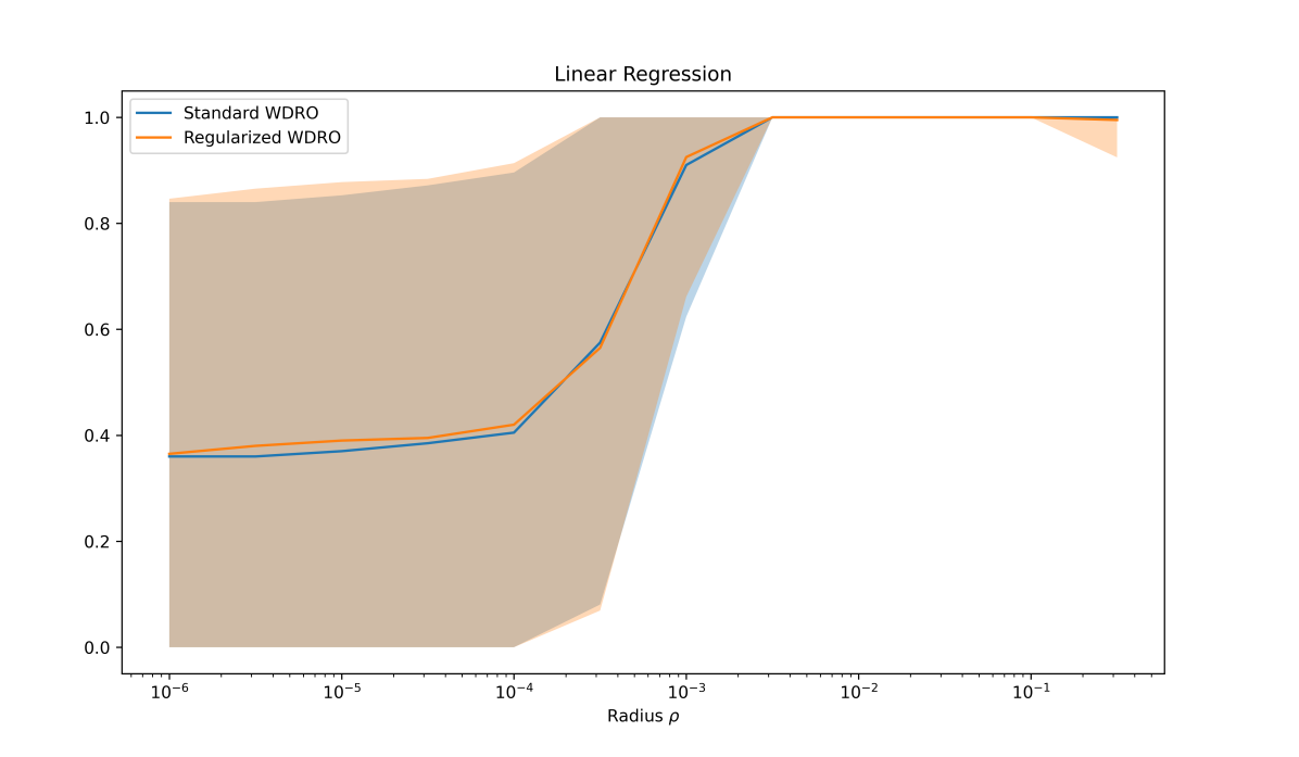
Estimates of the probability $P^{\otimes^{n}}\left(\widehat{\mathcal{R}}^{\epsilon}_{\rho^{2}}(f(\hat{\theta}_{n},\cdot))\geq\mathbb{E}_{P}[f(\hat{\theta}_{n},\xi)]\right)$ where $\hat{\theta}_{n}$ is the robust model with radius $\rho$ for the linear regression model (Example 3.7). $\theta$ has dimension $d=10$, $n=1000$ synthetic training samples are used, $\sigma$ and $\epsilon$ are chosen proportional to $\rho$ following Section 3.2. For each value of $\rho$, we sample 200 training datasets and solve the WDRO problem on each of them, to obtain an estimate of the probability above. The solid line is the average over these 200 results, while the shaded area represents the standard deviation. As predicted by Sections 3.1 and 3.2, we observe that for $\rho$ large enough, the probability that the robust loss on the training set upper bounds the true risk is almost 1. We also observe that standard and regularized WDRO have almost identical generalization behaviours. The WDRO problems are solved by LBFGS-B combined with the formulas of Example 2 of Wang et al. (2023).

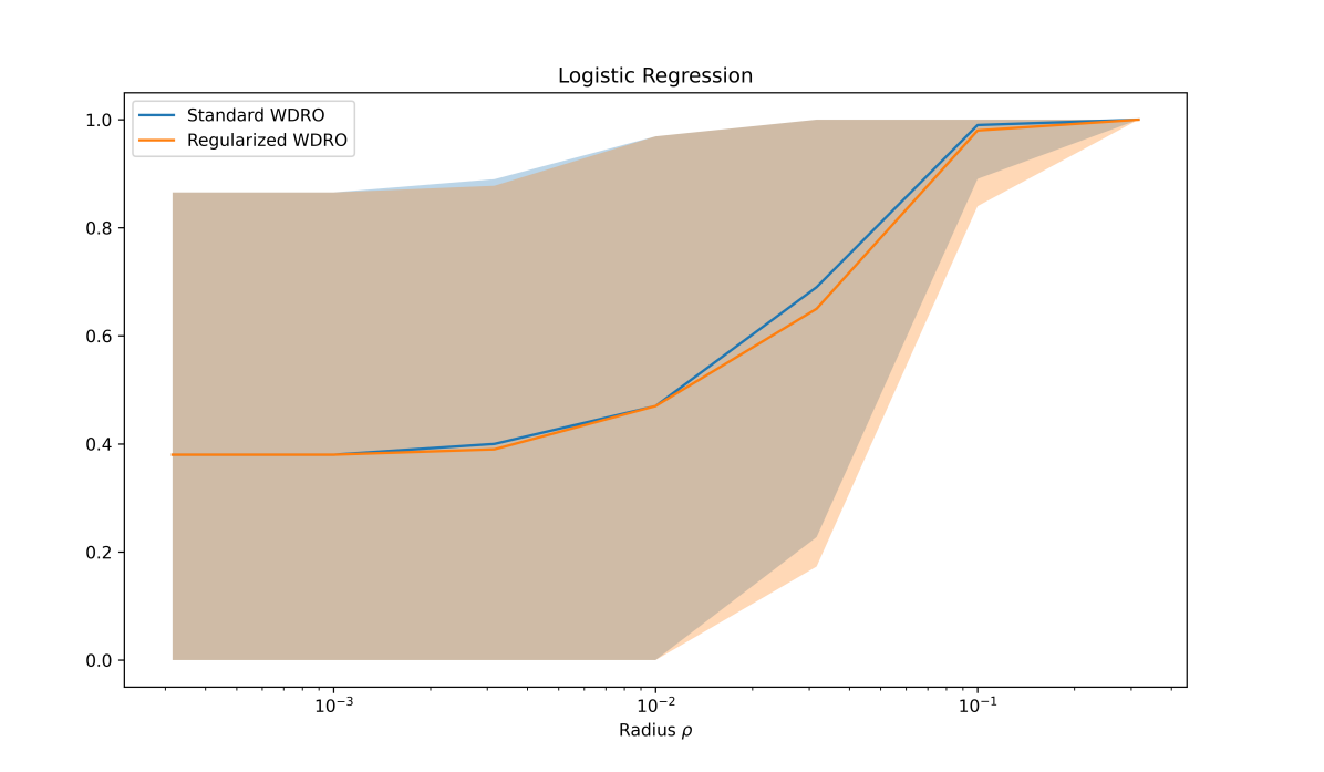
Estimates of the probability $P^{\otimes^{n}}\left(\widehat{\mathcal{R}}^{\epsilon}_{\rho^{2}}(f(\hat{\theta}_{n},\cdot))\geq\mathbb{E}_{P}[f(\hat{\theta}_{n},\xi)]\right)$ where $\hat{\theta}_{n}$ is the robust model with radius $\rho$ for the logistic regression model (Example 3.6). $\theta$ has dimension $d=5$, $n=500$ synthetic training samples are used, $\sigma$ and $\epsilon$ are chosen proportional to $\rho$ following Section 3.2. For each value of $\rho$, we sample 100 training datasets and solve the WDRO problem on each of them, to obtain an estimate of the probability above. The solid line is the average over these 100 results, while the shaded area represents the standard deviation. As for the previous plot and as predicted by Sections 3.1 and 3.2, we observe that for $\rho$ large enough, the probability that the robust loss on the training set upper bounds the true risk is almost 1. We also observe that standard and regularized WDRO have almost identical generalization behaviours. The standard WDRO problem is solved using the algorithm of Blanchet et al. (2022b) while the regularized problem is solved using LBFGS-B combined with an explicit expression of the inner integral in the robust loss.

References

• An and Gao (2021) Y. An and R. Gao. Generalization bounds for (wasserstein) robust optimization. Advances in Neural Information Processing Systems, 34:10382–10392, 2021.
• Arbel and Mairal (2022) M. Arbel and J. Mairal. Non-Convex Bilevel Games with Critical Point Selection Maps. Advances in Neural Information Processing Systems, 36:1–34, 2022.
• Arrigo et al. (2022) A. Arrigo, C. Ordoudis, J. Kazempour, Z. De Grève, J.-F. Toubeau, and F. Vallée. Wasserstein distributionally robust chance-constrained optimization for energy and reserve dispatch: An exact and physically-bounded formulation. European Journal of Operational Research, 296(1):304–322, 2022.
• Azizian et al. (2023) W. Azizian, F. Iutzeler, and J. Malick. Regularization for Wasserstein distributionally robust optimization. ESAIM: COCV, 29:33, 2023.
• Blanchet and Kang (2020) J. Blanchet and Y. Kang. Semi-supervised learning based on distributionally robust optimization. Data Analysis and Applications 3: Computational, Classification, Financial, Statistical and Stochastic Methods, 5:1–33, 2020.
• Blanchet and Murthy (2019) J. Blanchet and K. Murthy. Quantifying distributional model risk via optimal transport. Mathematics of Operations Research, 44(2):565–600, 2019.
• Blanchet and Shapiro (2023) J. Blanchet and A. Shapiro. Statistical limit theorems in distributionally robust optimization. arXiv preprint arXiv:2303.14867, 2023.
• Blanchet et al. (2021) J. Blanchet, K. Murthy, and V. A. Nguyen. Statistical analysis of wasserstein distributionally robust estimators. In Tutorials in Operations Research: Emerging Optimization Methods and Modeling Techniques with Applications, pages 227–254. INFORMS, 2021.
• Blanchet et al. (2022a) J. Blanchet, K. Murthy, and N. Si. Confidence regions in wasserstein distributionally robust estimation. Biometrika, 109(2):295–315, 2022a.
• Blanchet et al. (2022b) J. Blanchet, K. Murthy, and F. Zhang. Optimal transport-based distributionally robust optimization: Structural properties and iterative schemes. Mathematics of Operations Research, 47(2):1500–1529, 2022b.
• Boucheron et al. (2013) S. Boucheron, G. Lugosi, and P. Massart. Concentration Inequalities: A Nonasymptotic Theory of Independence. Oxford University Press, 2013.
• Boumal (2023) N. Boumal. An introduction to optimization on smooth manifolds. Cambridge University Press, 2023.
• Chen and Paschalidis (2018) R. Chen and I. C. Paschalidis. A robust learning approach for regression models based on distributionally robust optimization. Journal of Machine Learning Research, 19(13), 2018.
• Dapogny et al. (2023) C. Dapogny, F. Iutzeler, A. Meda, and B. Thibert. Entropy-regularized wasserstein distributionally robust shape and topology optimization. Structural and Multidisciplinary Optimization, 66(3):42, 2023.
• Delage and Ye (2010) E. Delage and Y. Ye. Distributionally Robust Optimization Under Moment Uncertainty with Application to Data-Driven Problems. Operations Research, 58:595–612, 2010.
• Esfahani and Kuhn (2018) P. M. Esfahani and D. Kuhn. Data-driven distributionally robust optimization using the wasserstein metric: Performance guarantees and tractable reformulations. Mathematical Programming, 171(1):115–166, 2018.
• Feydy et al. (2019) J. Feydy, T. Séjourné, F.-X. Vialard, S.-i. Amari, A. Trouvé, and G. Peyré. Interpolating between optimal transport and MMD using Sinkhorn divergences. In The 22nd International Conference on Artificial Intelligence and Statistics, pages 2681–2690. PMLR, 2019.
• Fournier and Guillin (2015) N. Fournier and A. Guillin. On the rate of convergence in wasserstein distance of the empirical measure. Probability Theory and Related Fields, 162(3):707–738, 2015.
• Gao (2022) R. Gao. Finite-sample guarantees for wasserstein distributionally robust optimization: Breaking the curse of dimensionality. Operations Research, 2022.
• Gao and Kleywegt (2016) R. Gao and A. J. Kleywegt. Distributionally robust stochastic optimization with wasserstein distance. Mathematics of Operations Research, 2016.
• Genevay et al. (2016) A. Genevay, M. Cuturi, G. Peyré, and F. Bach. Stochastic Optimization for Large-scale Optimal Transport. In NIPS 2016 - Thirtieth Annual Conference on Neural Information Processing System, Proc. NIPS 2016, 2016.
• Genevay et al. (2019) A. Genevay, L. Chizat, F. Bach, M. Cuturi, and G. Peyré. Sample complexity of sinkhorn divergences. In The 22nd International Conference on Artificial Intelligence and Statistics, pages 1574–1583. PMLR, 2019.
• Goh and Sim (2010) J. Goh and M. Sim. Distributionally Robust Optimization and Its Tractable Approximations. Operations Research, 58:902–917, 2010.
• Kuhn et al. (2019) D. Kuhn, P. M. Esfahani, V. A. Nguyen, and S. Shafieezadeh-Abadeh. Wasserstein distributionally robust optimization: Theory and applications in machine learning. In Operations Research & Management Science in the Age of Analytics. INFORMS, 2019.
• Kwon et al. (2020) Y. Kwon, W. Kim, J.-H. Won, and M. C. Paik. Principled learning method for wasserstein distributionally robust optimization with local perturbations. In International Conference on Machine Learning, pages 5567–5576. PMLR, 2020.
• Laguel et al. (2020) Y. Laguel, J. Malick, and Z. Harchaoui. First-order optimization for superquantile-based supervised learning. In 2020 IEEE 30th International Workshop on Machine Learning for Signal Processing (MLSP), pages 1–6. IEEE, 2020.
• Lee and Raginsky (2018) J. Lee and M. Raginsky. Minimax statistical learning with wasserstein distances. Advances in Neural Information Processing Systems, 31, 2018.
• Lee (2018) J. M. Lee. Introduction to Riemannian manifolds, volume 2. Springer, 2018.
• Levy et al. (2020) D. Levy, Y. Carmon, J. C. Duchi, and A. Sidford. Large-scale methods for distributionally robust optimization. Advances in Neural Information Processing Systems, 33, 2020.
• Li et al. (2020) J. Li, C. Chen, and A. M.-C. So. Fast Epigraphical Projection-based Incremental Algorithms for Wasserstein Distributionally Robust Support Vector Machine. In Advances in Neural Information Processing Systems, volume 33, pages 4029–4039. Curran Associates, Inc., 2020.
• Paty and Cuturi (2020) F.-P. Paty and M. Cuturi. Regularized Optimal Transport is Ground Cost Adversarial. In ICML, 2020.
• Peyré and Cuturi (2019) G. Peyré and M. Cuturi. Computational optimal transport: With applications to data science. Foundations and Trends® in Machine Learning, 11(5-6):355–607, 2019.
• Piat et al. (2022) W. Piat, J. Fadili, F. Jurie, and S. da Veiga. Regularized robust optimization with application to robust learning. 2022.
• Rockafellar and Wets (1998) R. T. Rockafellar and R. J.-B. Wets. Variational Analysis. Grundlehren Der Mathematischen Wissenschaften. Springer-Verlag, 1998.
• Rudin (1987) W. Rudin. Real and Complex Analysis. McGraw-Hill, 1987.
• Shafieezadeh Abadeh et al. (2015) S. Shafieezadeh Abadeh, P. M. Mohajerin Esfahani, and D. Kuhn. Distributionally Robust Logistic Regression. In Advances in Neural Information Processing Systems, volume 28. Curran Associates, Inc., 2015.
• Shafieezadeh-Abadeh et al. (2019) S. Shafieezadeh-Abadeh, D. Kuhn, and P. M. Esfahani. Regularization via Mass Transportation. Journal of Machine Learning Research, 20:1–68, 2019.
• Sinha et al. (2018) A. Sinha, H. Namkoong, and J. Duchi. Certifying some distributional robustness with principled adversarial training. In International Conference on Learning Representations, 2018.
• Song et al. (2023) J. Song, N. He, L. Ding, and C. Zhao. Provably convergent policy optimization via metric-aware trust region methods. arXiv preprint arXiv:2306.14133, 2023.
• Staib and Jegelka (2019) M. Staib and S. Jegelka. Distributionally robust optimization and generalization in kernel methods. Advances in Neural Information Processing Systems, 32, 2019.
• Wainwright (2019) M. J. Wainwright. High-dimensional statistics: A non-asymptotic viewpoint, volume 48. Cambridge university press, 2019.
• Wang and Xie (2022) J. Wang and Y. Xie. A data-driven approach to robust hypothesis testing using sinkhorn uncertainty sets. In 2022 IEEE International Symposium on Information Theory (ISIT), pages 3315–3320. IEEE, 2022.
• Wang et al. (2022) J. Wang, R. Moore, Y. Xie, and R. Kamaleswaran. Improving sepsis prediction model generalization with optimal transport. In Machine Learning for Health, pages 474–488. PMLR, 2022.
• Wang et al. (2023) J. Wang, R. Gao, and Y. Xie. Sinkhorn distributionally robust optimization. arXiv preprint arXiv:2109.11926, 2023.
• Zeng and Lam (2022) Y. Zeng and H. Lam. Generalization bounds with minimal dependency on hypothesis class via distributionally robust optimization. Advances in Neural Information Processing Systems, 35:27576–27590, 2022.
• Zhao and Guan (2018) C. Zhao and Y. Guan. Data-driven risk-averse stochastic optimization with wasserstein metric. Operations Research Letters, 46(2):262–267, 2018.
• Zhu et al. (2021a) J.-J. Zhu, W. Jitkrittum, M. Diehl, and B. Schölkopf. Kernel distributionally robust optimization: Generalized duality theorem and stochastic approximation. In International Conference on Artificial Intelligence and Statistics, pages 280–288. PMLR, 2021a.
• Zhu et al. (2021b) J.-J. Zhu, C. Kouridi, Y. Nemmour, and B. Schölkopf. Adversarially robust kernel smoothing. arXiv preprint arXiv:2102.08474, 2021b.