Vecchia Gaussian Process Ensembles on Internal Representations of Deep Neural Networks

Abstract

For regression tasks, standard Gaussian processes (GPs) provide natural uncertainty quantification, while deep neural networks (DNNs) excel at representation learning. We propose to synergistically combine these two approaches in a hybrid method consisting of an ensemble of GPs built on the output of hidden layers of a DNN. GP scalability is achieved via Vecchia approximations that exploit nearest-neighbor conditional independence. The resulting deep Vecchia ensemble not only imbues the DNN with uncertainty quantification but can also provide more accurate and robust predictions. We demonstrate the utility of our model on several datasets and carry out experiments to understand the inner workings of the proposed method.

Keywords: nearest neighbors; Vecchia approximation; Gaussian process ensemble

1 Introduction

In recent years, deep neural networks (DNNs) have achieved remarkable success in various tasks such as image recognition, natural language processing, and speech recognition. However, despite their excellent performance, these models have certain limitations, such as their lack of uncertainty quantification (UQ). Much of UQ for DNNs is based on a Bayesian approach that models network weights as random variables [22] or has involved ensembles of networks [18].

Gaussian processes (GPs) provide natural UQ, but they lack the representation learning that makes DNNs successful. Standard GPs are known to scale poorly with large datasets, but GP approximations are plentiful and one such method is the Vecchia approximation [31, 16], which uses nearest-neighbor conditioning sets to exploit conditional independence among the data. In high dimensions, finding the appropriate conditioning sets is challenging, so a procedure that can discover the conditional independence can expand the applicability of the Vecchia approximation.

While the literature on Bayesian neural networks and deep ensembles is rich, less has been done on using the outputs of internal layers of DNNs to quantify uncertainty for the neural network. In this paper we propose the deep Vecchia ensemble (DVE), which uses the outputs of internal layers in conjunction with the Vecchia approximation to provide UQ for DNNs. By using the outputs of internal layers of the DNN, we inject the representation learning of DNNs into GPs. As a result, we are able to use the DNN to discover better conditioning sets for the Vecchia approximation. A high-level summary of this approach is given in Figure 1, where the outputs of internal layers are given in the bottom right three panels and the different conditioning sets extracted from the neural network are shown in the panel on the left.

We believe that the proposed methodology has the potential to improve the reliability and robustness of deep learning models in various applications while simultaneously improving Vecchia GPs. The remainder of the paper is organized as follows: We begin in Section 2 with a review of related concepts and define the intermediate representations upon which we later build. In Section 3, we contextualize our approach within existing work on uncertainty quantification for neural networks and GP approximation. The proposed methodology is detailed in Section 4. We then apply our model to pretrained neural networks in Section 5. This is followed by an experiment in Section 6 that explores how our model works. In Section 7, we discuss potential application areas for our method, the limitations of our approach, and future research directions that could improve upon our work.

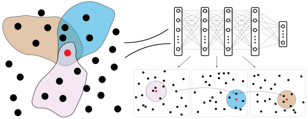
Figure 1: Nearest-neighbor conditioning sets for different input representations obtained via the layers of a DNN. Left: The red point has different nearest-neighbor conditioning sets based on the metric induced by the internal representations of the neural network. The brown, blue, and pink shaded areas denote the regions in input space that will be mapped to a hypersphere in the first, second, and third intermediate spaces, respectively. The conditioning sets derived from the different regions may overlap, as in the blue and brown region, or be disjoint from the others as in the pink region. Right: The data used to train the network is mapped through each layer and the output, or feature map, of each datum is stored. For a red test point, we asses uncertainty by asking: How many instances in the training data took similar paths through the network?

2 Preliminaries

In this section, we provide background information on GPs, including GP regression, as well as the Vecchia approximation to GPs. We also review GP ensembles, which combine multiple GPs to provide a distribution over the response variable. Finally, we define internal spaces as intermediate representations of the input data generated by the neural network.

2.1 Modeling functions with Gaussian processes

Suppose we have a dataset $\mathcal{D}=\{\bm{X},\bm{y}\}=\{\bm{x}_{i},y_{i}\}_{i=1}^{n}$, where $\bm{x}_{i}\in\mathcal{X}$, $y_{i}=f(\bm{x}_{i})+\epsilon_{i}$, $\epsilon_{i}\stackrel{{\scriptstyle iid}}{{\sim}}\mathcal{N}(0,\sigma^{2})$, and $f:\mathcal{X}\rightarrow\mathbb{R}$. Our goal is to make predictions at $n_{p}$ test locations $\bm{X}^{*}=\{\bm{x}^{*}_{j}\}_{j=1}^{n_{p}}$ in a probabilistic fashion. A common approach is to assign the latent function $f$ a zero-mean Gaussian process prior with covariance function $K_{\bm{\theta}}(\bm{x},\bm{x}^{\prime})$ parameterized by $\bm{\theta}$. Letting $\bm{y}^{*}=\{f(\bm{x}^{*}_{j})+\epsilon_{j}\}_{j=1}^{n_{p}}$, $p(\bm{y}^{*},\bm{y})$ will be jointly multivariate normal, which implies:

$$p(\bm{y}^{*}|\bm{y})=\mathcal{N}(\bm{\mu}^{*},\bm{K}_{\bm{\theta}^{*}}+\sigma^{2}\bm{I}_{n_{p}}),$$ (1)

where $\bm{\mu}^{*}$ and $\bm{K}_{\bm{\theta}^{*}}$ depend on $\mathcal{D}$ and $\bm{\theta}$. To select $\bm{\theta}^{*}$, we maximize the marginal log-likelihood:

$$p(\bm{y}) =\int p(\bm{y}|\bm{f})p(\bm{f})d\bm{f}=\mathcal{N}(\bm{0},\bm{K}_{\bm{\theta}}(\bm{X},\bm{X})+\sigma^{2}\bm{I}_{n}).$$ (2)

Both Equation (1) and (2) have time and space complexities of $\mathcal{O}(n^{3})$ and $\mathcal{O}(n^{2})$, respectively.

2.2 Approximating Gaussian processes using Vecchia

The joint distribution of a collection of random variables, $\bm{y}=\{y_{1},y_{2},...,y_{n}\}$, can be decomposed as $p(\bm{y})=\prod_{i=1}^{n}p(y_{i}|\bm{y}_{h(i)})$, $h(i)=\{1,...,i-1\}$. Vecchia’s approximation [31] conditions the $i^{th}$ observation on a set indexed by $g(i)$, with $g(i)\subset h(i)$. The approximate joint distribution is then,

$$p(\bm{y}) \approx\prod_{i=1}^{n}p(y_{i}|\bm{y}_{g(i)}).$$ (3)

Letting $\tilde{\bm{y}}=(\bm{y},\bm{y}^{*})$, where $\bm{y}^{*}=\{y^{*}_{n+1},...,y^{*}_{n+n_{p}}\}$ are test points ordered after the observed data, the approximate conditional distribution for $\bm{y}^{*}$ is:

$$p(\bm{y}^{*}|\bm{y}) \approx\prod_{j=n+1}^{n+n_{p}}p(y^{*}_{j}|\tilde{\bm{y}}_{g(j)}).$$ (4)

For fixed $g(i)$’s, such that $|g(i)|\leq m$ with $m\ll n$, the approximation in (3) reduces the in-memory space complexity of Equation (2) to $\mathcal{O}(n_{p}m)$. Using the approximation in Equation (4) reduces the time and space complexity of Equation (1) to $\mathcal{O}(n_{p}m)$. An additional approximation utilizing mini-batches [14] of size $n_{b}$ results in an in-memory space complexity of $\mathcal{O}(n_{b}m^{2})$ for Equation (2) and a time complexity of $\mathcal{O}(n_{b}m^{3})$.

For the $i^{th}$ data point, the $m$ ordered nearest neighbors $g(i)$ are typically determined based on a distance metric, such as Euclidean distance, between the input variables $\bm{x}$. To compute these ordered nearest neighbors, it is assumed that the data has been sorted according to some ordering procedure, and for each $i$, the $m$ nearest neighbors that precede $i$ in the ordering are selected.

2.3 Ensembling Gaussian processes

An ensemble of $L$ GPs can be formed by partitioning the training data into disjoint subsets and fitting independent GPs to each subset of the training data. Assuming this independence structure, the hyperparameters, $\bm{\theta}_{k}$, can be learned by maximizing the log-marginal likelihood, $\sum_{k=1}^{L}\text{log }p_{k}(\bm{y}^{(k)}|\bm{\theta}_{k})$.

While in this work we allow each GP to have its own hyperparameters, product-of-expert GP ensembles [30, 3, 7, 26] typically share hyperparameters $\bm{\theta}$ between the GPs. We are assuming $\bm{\theta}_{k}$ contains all the hyperparameters in both the GP kernel and the likelihood.

The prediction of $y^{*}$ at a location $\bm{x}^{*}$ can be formed by using a generalized product of experts (gPoE) [3], an extension of product of experts (PoE) [13], which combines the predictions of $L$ models by using a weighted product of the predictions. Letting $p_{k}^{\beta_{k}(\bm{x}^{*})}(y^{*})$ denote the $k^{th}$ model’s predictive distribution for $y^{*}$, the combined distribution for $y^{*}$ is given by,

$$p(y^{*}) \propto\prod_{k=1}^{L}p_{k}^{\beta_{k}(\bm{x}^{*})}(y^{*}).$$ (5)

The function $\beta_{k}(\bm{x}^{*})$ is a weight for the $k^{th}$ model’s prediction based on the input $\bm{x}^{*}$ such that $\sum_{k=1}^{L}\beta_{k}(\bm{x}^{*})=1$. When each of the $k$ predictions is a Gaussian distribution with mean $\mu_{k}(\bm{x}^{*})$ and variance $\bm{\sigma}_{k}(\bm{x}^{*})$, the combined distribution is also Gaussian with combined mean and variance given by,

$$\mu(\bm{x}^{*}) =\sigma^{2}(\bm{x}^{*})\sum_{k=1}^{L}\beta_{k}(\bm{x}^{*})\sigma^{-2}_{k}(\bm{x}^{*})\mu_{k}(\bm{x}^{*}),\hskip 28.45274pt\sigma^{2}(\bm{x}^{*})=(\sum_{k=1}^{L}\beta_{k}(\bm{x}^{*})\sigma^{-2}_{k}(\bm{x}^{*}))^{-1}.$$ (6)

For details on computing $\beta_{k}$ see Appendix F.

Although we have focused on the combined predictive distribution for the observed $y^{*}$, in the case of a Gaussian likelihood the same results hold for the combined distribution of the latent function $f^{*}$ (with the variance terms changed to reflect we are working with the noiseless latent function). This implies we can choose to combine in either $f$ or $y$ space. For details on this see Appendix G.

2.4 Extracting information from intermediate representations

Consider a finite sequence of functions $f_{1},...,f_{L+1}$ such that $f_{1}:\mathbb{R}^{d}\rightarrow\mathcal{A}_{1}$, $f_{2}:\mathcal{A}_{1}\rightarrow\mathcal{A}_{2}$, …,$f_{L}:\mathcal{A}_{L-1}\rightarrow\mathcal{A}_{L}$, $f_{L+1}:\mathcal{A}_{L}\rightarrow\mathbb{R}$, where each $\mathcal{A}_{i}\subset\mathbb{R}^{d_{i}}$.

The $k^{th}$ intermediate representation of a point $\bm{x}\in\mathbb{R}^{d}$ with respect to the sequence $f_{1},...,f_{L+1}$ is defined to be $\bm{e}_{k}(\bm{x}):=(f_{k}\circ f_{k-1}\circ...\circ f_{1})(\bm{x})$. The $k^{th}$ intermediate space $\mathcal{A}_{k}$ is the image of $(f_{k}\circ f_{k-1}\circ...\circ f_{1})(\cdot)$. A composite model $\mathcal{M}$ is the composition of $L$ such functions $M(\bm{x}):=(f_{L+1}\circ f_{L-1}\circ...\circ f_{2}\circ f_{1})(\bm{x})$. A feed-forward neural network with $L$ layers is an example of a composite model and the output of each layer in the network, excluding the final layer, results in an intermediate space.

3 Related work

We summarize work on improving scalability of GPs, quantifying uncertainty of neural networks, and using the outputs of internal layers of a neural network.

There are several common directions of research that have focused on scaling GPs. The most relevant for our work are the Vecchia approximation [31, 16], inducing-point GPs [12, 29], and ensembling methods [30, 7, 3]. The Vecchia approximation is based on an ordered conditional approximation of joint distributions, where conditioning sets are often computed using nearest neighbors, which is difficult in high input dimensions. Inducing point methods assume that the covariance matrix has a low-rank structure but they can result in overly smooth approximations. Finally, ensembling methods assign an independent GP to partitions of the data, and while this greatly improves scalability, much work has been done on improve and understanding the failure modes of these models [5, 26].

The work on uncertainty quantification (UQ) for deep learning most relevant to our paper are those involving ensembles of deep neural networks (DNNs) [18] and those using Bayesian neural networks (BNNs) [22]. Ensemble-based methods independently train DNNs on subsamples of the data. BNNs take the weights of the neural network to be random variables and use Bayes’ rule to derive a posterior for the weights given the data. Each realization of the weights from the posterior implies a different network. By marginalizing over the posterior when forming predictions, the uncertainty in the weights is propagated to the uncertainty in the prediction. The posterior is rarely available in closed form and therefore we rely on approximate sampling or posterior approximation [22, 21, 4, 8]. Both BNNs and ensembles of DNNs consider multiple networks, but in this work we use a single network at a time. Therefore, our work can always be used within either framework and should not be taken as alternative to these methods, but simply as an extension.

In this work we heavily use the outputs of internal layers of DNNs, which has been done for explainable AI [2], deep kernel learning [32], deep Gaussian process [6] and within Resnet [11]. For explainable AI, the goal is to understand what features the network is learning to extract. Resnet’s skip connections ensure, among other things, that adding new layers doesn’t reduce the class of functions the network can model. However, neither of these two approaches use the outputs of the internal layers for UQ of DNNS or to improve GP approximations. While deep kernel learning is closest to our work, we use more than just the final layer which we believe is critical for uncertainty quantification and predictive performance (see the S-curve example in Section 6). Finally, unlike the deep Gaussian process, we are not feeding the output of one GP into the next, but instead feeding the output of network layers into Vecchia GPs.

4 Proposed methodology

This section outlines our proposed methodology, beginning with a concise model summary. We then describe our approach for extracting a sequence of datasets from a pretrained neural network, followed by a discussion of our conditioning set computation process. Next, we detail our method for building an ensemble using the collections of conditioning sets. Throughout, we explain the design choices that informed the development of our model.

4.1 Model summary

We are provided with a dataset $\mathcal{D}$ comprising $n$ input-output pairs, $\mathcal{D}=\{\bm{x}_{i},y_{i}\}_{i=1}^{n}$, and a composite model $\mathcal{M}:\mathcal{X}\rightarrow\mathbb{R}$ that is trained to predict $y_{i}$ given the corresponding $\bm{x}_{i}$. Initially, we map the inputs $\{\bm{x}_{i}\}_{i=1}^{n}$ to their respective intermediate representations, $\{\bm{e}_{k}(\bm{x}_{i})\}_{i=1}^{n}$, where $k=1,...,L$. We generate a collection of conditioning sets, $\mathcal{G}_{k}$, for each set of intermediate representations, $\{\bm{e}_{k}(\bm{x}_{i})\}_{i=1}^{n}$, by computing ordered nearest neighbors based on the Euclidean distance between the intermediate representations. The resulting tuple for each intermediate space $(\{\bm{e}_{k}(\bm{x}_{i}),\bm{y}_{i}\}_{i=1}^{n},\mathcal{G}_{k})$ is combined with an automatic relevance determination (ARD) kernel $K_{\bm{\theta}_{k}}(\cdot,\cdot)$ of the appropriate dimension to form an ensemble of deep Vecchia Gaussian processes (GPs).

At test time, the test point will be mapped to its intermediate spaces and each Vecchia GP will provide a predictive mean and variance. The predictions are then combined via a product of experts to form a single mean and covariance estimate. The diagram in Figure 2 provides a high-level overview of the proposed model.

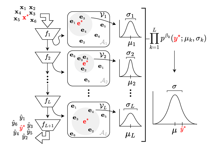
Figure 2: The input data $\bm{x}_{1},\bm{x}_{2},\bm{x}_{3},\ldots$ are fed into the network, and the output of each intermediate layer creates a new intermediate space (e.g., $\mathcal{A}_{1}$). Within each intermediate space, we can consider the nearest neighbors of any point in the space. For example, in the box labeled $\mathcal{A}_{1}$, we see that the red test point ${\color[rgb]{1,0,0}x^{*}}$ is closest to $\bm{e}_{1},\bm{e}_{3},\bm{e}_{4}$ (in the first intermediate space), and in $\mathcal{A}_{2}$, the closest points to ${\color[rgb]{1,0,0}x^{*}}$ are $\bm{e}_{2},\bm{e}_{3},\bm{e}_{4}$. We define $L$ Vecchia GPs, denoted by $\mathcal{V}_{1},\ldots,\mathcal{V}_{L}$, which estimate a distribution over the response using the nearest neighbors in their respective intermediate spaces. The resulting distributions are combined in a product-of-experts fashion to yield a single distribution parameterized by $\hat{\mu}$ and $\hat{\sigma}$. Although the neural network generates a point estimate ${\color[rgb]{1,0,0}\hat{y}^{*}}$ for the value of ${\color[rgb]{1,0,0}y^{*}}$, our method provides a distribution that better reflects the uncertainty in the prediction.

4.2 Dataset extraction from a neural network

To begin we describe how we extract a sequence of datasets from a pretrained neural network and the data it was trained on. Suppose the first layer of our pretrained network is of the form $f_{1}(\bm{x})=\sigma(\bm{x}^{T}\bm{W}^{(1)}+\bm{b}^{(1)})$, with, $\bm{W}^{(1)}\in\mathbb{R}^{dxd_{1}}$, $\bm{b}_{1}\in\mathbb{R}^{d_{1}}$ and $\sigma_{1}:\mathbb{R}^{d_{1}}\rightarrow\mathbb{R}^{d_{1}}$. Then $\bm{x}$’s first intermediate representation, $\bm{e}_{1}(\bm{x}):=f_{1}(\bm{x})$, will lie in a subset of $\mathbb{R}^{d_{1}}$, that is $\bm{e}_{1}(\bm{x})\in\mathcal{A}_{1}\subset\mathbb{R}^{d_{1}}$. Similarly, $\bm{x}$’s second intermediate representation is given by, $\bm{e}_{2}(\bm{x}):=(f_{2}\circ f_{1})(\bm{x})$, where $f_{2}(\bm{e}_{2}(\bm{x}))=\sigma(\bm{e}_{2}(\bm{x})\bm{W}^{(2)}+\bm{b}^{(2)})$ with $\bm{W}^{(2)}\in\mathbb{R}^{d_{1}xd_{2}}$, $\bm{b}_{2}\in\mathbb{R}^{d_{2}}$ and $\sigma_{2}:\mathbb{R}^{d_{2}}\rightarrow\mathbb{R}^{d_{2}}$. We can define the remaining $L-2$ intermediate representations in a similar way and by combining the intermediate representations with the responses we can generate $L$ datasets $\{\mathcal{D}_{k}\}_{k=1}^{L}$ where $\mathcal{D}_{k}=\{\bm{e}_{k}(\bm{x}_{i}),y_{i}\}_{i=1}^{n}$. We assume the same ordering of observations for all $L$ datasets, so $y_{i}$ will always refer to the same response for every $\mathcal{D}_{k}$.

An example of generating $L$ datasets is visualized in Figure 3 for the bike UCI dataset. Each of the panels contains one dataset to which we fit a Vecchia GP.

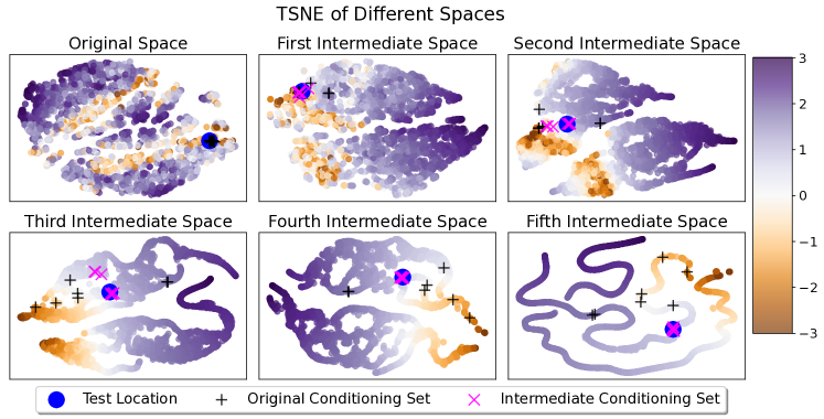
Figure 3: The 2D TSNE projection of input points in the original space of the bike UCI dataset (top left panel) and intermediate spaces (remaining five panels) with the color denoting the response value corresponding to each point. The blue dot is a fixed test point that has been propagated through the network. The black crosses denote the ordered nearest neighbors of the blue dot in the original input space, and their corresponding intermediate representations. The magenta crosses denote the ordered points nearest to the blue point within each intermediate space.

4.3 Conditioning-set selection

Figure 3 suggests that the function $\bm{e}_{k}(\bm{x})\mapsto y$ may be smooth and therefore we choose to estimate this function using a Gaussian process. For computational purposes, we approximate each of the GPs using Vecchia with nearest neighbors computed in the corresponding intermediate space. Doing so gives rise to several conditioning sets for each observation $\bm{x}_{i}$.

For example, consider the $i^{th}$ input $\bm{x}_{i}$ and its previously ordered nearest neighbors. In Figure 3 $\bm{x}_{i}$ is given by the blue dot in the upper left most panel and the black crosses are $\bm{x}_{i}$’s previously ordered nearest neighbors. As $\bm{x}_{i}$ and its nearest neighbors are mapped to their first intermediate representations, we see that $\bm{x}_{i}$’s new nearest neighbors (the magenta crosses) are different than the original conditioning set. The magenta crosses in each subsequent panel represent $\bm{x}_{i}$’s previously ordered nearest neighbors in the corresponding intermediate space. The magenta crosses changes from panel to panel, giving different conditioning sets as $\bm{x}_{i}$ moves through the network.

Letting $g_{k}(i)$ denote the conditioning set for observation $i$ from intermediate space $k$, we can consider the collection of conditioning sets, which we denote by $\mathcal{G}_{k}:=\{g_{k}(1),...,g_{k}(n)\}$. An $L+1$ layer network will have $L$ collections of conditioning sets, $\mathcal{G}_{1},...,\mathcal{G}_{L}$. By using several collections of conditioning sets, we are utilizing the unique information present in the panels titled ‘First Intermediate Space’ through ‘Fifth Intermediate Space’. This approach can lead to better predictions compared to using just one collection of conditioning sets.

4.4 Ensemble building from conditioning sets

Each $\mathcal{G}_{k}$ represents a hypothesis about the conditional independence structure of the data. For instance, with time series data produced by an AR(2) process, the $i^{th}$ observation should depend on the two preceding observations in time, while for an AR(1) process, the conditioning set is limited to the immediately preceding data point. However, in general, it is unclear which $\mathcal{G}_{k}$ is most appropriate.

Since we do not know which $\mathcal{G}_{k}$ is most suitable, we propose an ensemble of Vecchia GPs, each of which is based on one of the collections of conditioning sets. With each Vecchia GP independently fit to its corresponding dataset (e.g. $\mathcal{D}_{k}$), we combine the predictions from each member of the ensemble in a product-of-experts fashion. Details on training and prediction are provided in Appendix A.

5 Application to pretrained models

We report results using networks that were pretrained on a collection of UCI regression tasks and a network pretrained for a face age estimation task. In each case, we compare our results to those obtained with the original network, and, where appropriate, we also compare against other GP-based methods, such as SVI-GP. All GPs use an ARD Matern 3/2 kernel. We assess performance using root mean square error (RMSE) and negative log-likelihood (NLL) on the standardized test data for the UCI regression tasks. We use the mean absolute error (MAE) on the original scale for face age estimation. We combine our predictions in $y$-space and details on this choice are given in Appendix G.

5.1 UCI benchmarks

We trained a feed-forward neural network on three train-validation-test splits of UCI regression tasks. After training, we constructed the deep Vecchia ensemble as detailed in Section 4 and made predictions for the test set using the method described in Appendix A. Additionally, we trained the stochastic variational inference GP (SVI-GP) of [12] and the scaled Vecchia GP of [17] separately on the training data for prediction on the test set.

Table 1 compares NLL (left column under each dataset) and RMSE (right column under each dataset) for different methods on UCI datasets. The bold value in each column is the best performing (lower is better). The value in parentheses is the sample standard deviation of the mean of the metric over the three different data splits. The last line of the table specifies the sample size ($n$) and dimension ($d$) for each dataset. Our method is given by ”DVE”, ”Neural Net” represents the original neural network, ”Vecchia” stands for the scaled Vecchia model of [17], and SVI-GP is the model from [12].

We can see that DVE performs the best among all given models in terms of NLL and is second only to the neural network in RMSE on two datasets. Of course the DVE estimates are built upon the network, but it is remarkable how the DVE is able to provide uncertainty estimates to the neural network’s predictions, providing much better performance than existing GP approximations.

Table 1: NLL (left columns) and RMSE (right columns) on UCI benchmarks

Method	Kin40K		Elevators		KEGG		bike		Protein
DVE	-1.445 (0.011)	0.057 (0.001)	0.424 (0.016)	0.373 (0.007)	-1.021 (0.030)	0.087 (0.002)	-3.154 (0.109)	0.010 (0.002)	0.646 (0.029)	0.494 (0.014)
Neural Net	N/A	0.069 (0.000)	N/A	0.363 (0.006)	N/A	0.085 (0.002)	N/A	0.018 (0.001)	N/A	0.514 (0.042)
Vecchia	-0.028 (0.015)	0.209 (0.015)	0.525 (0.015)	0.414 (0.006)	-0.987 (0.026)	0.090 (0.002)	-0.239 (0.010)	0.183 (0.001)	0.851 (0.003)	0.571 (0.002)
SVI-GP	-0.093 (0.008)	0.068 (0.005)	0.455 (0.017)	0.381 (0.007)	-0.912 (0.033)	0.098 (0.003)	-1.140 (0.047)	0.073 (0.004)	1.083 (0.001)	0.713 (0.001)
($n$,$d$)	(40K,8)		(16.6K,18)		(48.8K,20)		(17.4K, 17)		(45.7K,9)

5.2 Face age estimation

We now use our deep Vecchia ensemble with a pretrained network for face age estimation. Face age estimation involves predicting the age of a subject in a photograph. The moving window regression (MWR) of [27] is a CNN-based approach that uses ordinal regression to solve this problem.

The MWR procedure uses a CNN to extract features of a test image as well as two references images. These features are concatenated together and fed into a feedforward neural network, called a $\rho$-regressor, to predict the age of the test image relative to the reference images. We use the pretrained global $\rho$-regressor for the UTKFace dataset from [27] to form the intermediate representations of a deep Vecchia ensemble as described in Section 4.1. For more details on the MWR procedure, the UTKFace dataset, our processing and comparisons, see Appendix D.

In Table 2, we compare the results of the original global model (Global $\rho$-regressor), the deep Vecchia ensemble (DVE), a scaled Vecchia GP [17] fit to the output of the second to last layer (Vecchia) and the SVI-GP of [12] (SVI-GP) also fit to the outputs of the second-to-last layer. The latter two approaches can be viewed as variants of deep-kernel GPs.

By using the deep Vecchia ensemble, we were able to decrease the MAE for the global model and additionally provide an estimate of the model’s uncertainty. The NLL for the deep ensemble also outperformed the models that provided estimates of uncertainty. The difference in NLL and MAE between the Vecchia GP on the second-to-last layer and the deep ensemble Vecchia supports our claim that there is value in using the information in the intermediate layers for both predictions and uncertainty quantification.

Table 2: MAE and NLL for UTKFace dataset

	MAE	NLL
Global $\rho$-Regressor	4.650	N/A
DVE	4.636	1.085
SVI-GP	4.661	2.450
Vecchia	4.693	1.789

6 Exploring intermediate spaces

In this section we investigate the intermediate spaces of a small network to understand how the deep Vecchia ensemble is using different layers. We fit a feed forward network to samples from the S-curve dataset [28]. In the bottom row of Figure 4, we visualize the internal representations of the network. In the top row of Figure 4, we visualize the original data and the predictions formed by the deep Vecchia ensemble and the neural network. For more details, see Appendix E.

The first internal representation had more separation between yellow and green points compared to the final representation, indicating the earlier layer held information distilled away by the final layer. Deep Vecchia ensemble preserved this information, while the neural network discarded it. The deep Vecchia prediction closely resembled the original dataset, supported by lower RMSE values compared to the neural network’s prediction. We believe a similar phenomenon is occurring with the models used in Section 5.

To check whether the observed behavior held more generally we repeated the experiment using different networks and for every network we checked the results was the same. For example, with four hidden layers with (10, 5, 2, 2) units, the RMSE dropped from 0.18 to 4.2e-5. Changing the number of units per layer to (16,8,4,4) showed the RMSE drop from 0.007 to 3.9e-5.

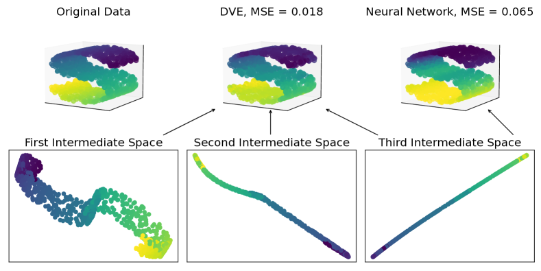
Figure 4: This figure shows the original data from the S-curve dataset in the top left panel. The top middle panel depicts the predictions generated by the deep Vecchia Ensemble, while the top right panel shows the predictions from the neural network. The three panels in the bottom row show the internal representations of the data from the three hidden layers of the network. The color of the points in each of these panels corresponds to the response value. The arrows pointing to the deep Vecchia prediction emphasize that the deep Vecchia ensemble builds predictions from all three layers. In contrast, the final network prediction relies on just the final layer, as indicated by the single arrow pointing to it.

6.1 Interpreting internal representations

Our model can be seen from two perspectives: an ensembling of Vecchia GPs, and a method for quantifying epistemic uncertainty in neural networks. Below we relate both view points to the results in this section.

From the Vecchia ensemble stance, we can see the intermediate representations in Figure 4 as providing three different distance metrics that can be used to compute possibly unique conditioning sets. The requirements to make this connection are formalized in Proposition 1. The proof of which can be found in Appendix B:

Proposition 1.

Consider a sequence of injective functions $f_{1},..,f_{L},f_{L+1}$ and a sequence of metric spaces $\{(M_{i},d_{i})\}_{i=1}^{L+1}$ such that $f_{i}:\mathcal{M}_{i}\rightarrow\mathcal{M}_{i+1}$ for $i=1,...,L$. Then $\{(M_{i},\tilde{d}_{i})\}_{i=2}^{L+1}$ defines a sequence of metric spaces, where $\tilde{d}_{i}(x,y):=d_{i}(\bm{e}_{i}(\bm{x}),\bm{e}_{i}(\bm{x}^{\prime}))$ for any $\bm{x},\bm{x}^{\prime}\in M_{1}$, with $\bm{e}_{i}(\bm{x}):=f_{i}\circ f_{i-1}\circ...\circ f_{1}(\bm{x})$ .

Proposition 1’s requirement that the function be injective ensures unique internal representations for unique input points, but continuity is not required. Discontinuous layers are useful when modeling functions with high Lipschitz constants or discontinuities. In such cases, predicting values using Euclidean nearest neighbors in $\mathbb{R}^{d}$ can be inaccurate, but the function may be continuous with respect to a different distance metric on $\mathbb{R}^{d}$. The difference in continuity is reminiscent of what we observed in Figure 3, where the function became progressively smoother for later intermediate spaces. While a similar goal is accomplished using deep kernels, by using multiple intermediate spaces we allow for competing hypothesis about what distance metric is best to be used.

From the perspective of uncertainty in neural networks, we can see the sequence of distance metrics as measuring how far a test point is away from instances in the training data. Of course, if a test point is close to existing training data with respect to the entire sequence of distance metrics, then the ensemble of Vecchia GPs will provide an estimate with small uncertainty estimates. If the test point is out of distribution, then the internal representations will not match existing data and we will return something close to the GP prior.

7 Conclusion

We presented an approach for UQ of pretrained neural networks. Our model has the added benefit of improving the Vecchia approximation and is the first approach to ensemble over the conditioning sets of the Vecchia approximation. The effectiveness of the model was shown on benchmark regression tasks and face age estimation. The study on internal representations provided insight into the inner workings of the approach.

We believe that our approach can find success in latent space Bayesian optimization [9] procedures that use a neural network to map latent representations to the response of interest, especially if the map between the latent space and the objective is not smooth. Our approach may reduce the need to provide additional structure to the latent space to allow for GP regression such as in [10]. We also believe that our method would work well in any application where nearest neighbors cannot be computed using Euclidean distance between inputs alone, such as high-dimensional regression.

Our proposed model has four key limitations. First, we need the data used to train the network which may not always be available. One possible solution is to simultaneously fit the network and an ensemble inducing-point GPs or to use a smaller validation set to build the deep Vecchia ensemble. The second limitation is that we combined predictions in $y$-space, so we are limited to using a Gaussian likelihood. This can be remedied by combining in $f$-space and defining a procedure to combine the noise terms in each of the Vecchia GP’s likelihoods. The third limitation is that we use a DNN with fixed weights but many BNN methods assume the weights are random variables. To incorporate the DVE into BNNs, each intermediate representation can be expressed by a distribution rather than a point estimate. Then an error-in-variables Vecchia GP can be made by combining the kernel from [1] with the correlation Vecchia strategy of [15]. The final limitation is that our exploration was limited to feed-forward layers. To extend our model to more general architectures, a distance metric between layer outputs can be defined to make our approach applicable.

Given our promising results and a clear path towards solving our current limitations, we believe the deep Vecchia ensemble should be adopted more broadly, and we would be excited to see others improve upon our work.

Appendix A Ensemble Training and Prediction

Training:
For an $L+1$ layer network, we obtain an ensemble of $L$ Vecchia GPs, each with its own set of parameters $\bm{\theta}_{k}=(\sigma_{k}^{2},\bm{\lambda}_{k},\tau_{k})$, where $\sigma_{k}^{2}$ denotes the output variance for the kernel, $\bm{\lambda}_{k}\in\mathbb{R}_{+}^{d_{k}}$ denotes the lengthscales for the ARD kernel, and $\tau_{k}^{2}$ denotes the variance in a Gaussian likelihood. To estimate $\bm{\theta}_{k}$ for each Vecchia GP, we independently employ mini-batch gradient descent within type-II maximum likelihood, optimizing the Vecchia marginal log-likelihood using the corresponding dataset $\mathcal{D}_{k}$:

$$\hat{\bm{\theta}}_{k} =\underset{\bm{\theta}\in\Theta}{\arg\max}\sum_{i=1}^{n}\text{ log }p_{k}(y_{i}|\bm{x}_{i},\bm{X}_{g_{k}(i)},\bm{y}_{g_{k}(i)},\bm{\theta}_{k})$$ (7)

The conditional distribution $p_{k}(y_{i}|\bm{y}_{g_{k}(i)},\bm{\theta}_{k})$ depends on the parameters $\bm{\theta}_{k}$, the intermediate representation, and the conditioning set. This model allows us to effectively capture the unique complexities present in each intermediate space of the neural network. Since we are optimizing the layerwise Vecchia GPs independently, we ignore the hierarchical structure of the intermediate representations. Training the models independently is fundamentally different from a deep Gaussian process [6] as we do not feed the outputs of one GP into the next GP. However, by performing our training in this way, we can more easily work with existing pretrained models. Therefore, our procedure can be viewed as augmenting both the Vecchia GP and the pretrained model.

Prediction:
For a test point $\bm{x}^{*}$, we compute the intermediate representation, $\bm{e}_{k}^{*}:=\bm{e}_{k}(\bm{x}^{*})$, and find the $m$ nearest neighbors of $\bm{e}_{k}^{*}$ in the dataset $\mathcal{D}_{k}$. We then compute the posterior mean $\mu_{k}^{*}$ and variance $\sigma_{k}^{*}$ of $f^{*}$, where $y^{*}|f^{*}\sim\mathcal{N}(f^{*},\sigma_{k}^{2})$. We repeat this for each of the $L$ layers. We then combine the $L$ estimates into a single estimate as given below:

$$\mu(\bm{x}^{*}) =\sigma^{2}(\bm{x}^{*})\sum_{k=1}^{L}\beta_{k}(\bm{e}_{k}^{*})(\sigma_{k}^{*})^{-2}\mu_{k}^{*}\hskip 28.45274pt\sigma^{2}(\bm{x}^{*})=\sum_{k=1}^{L}\beta_{k}(\bm{e}_{k}^{*})(\sigma_{k}^{*})^{-2}$$ (8)

We chose this combining strategy to account for prediction uncertainty. Specifically, our approach implicitly considers the degree of agreement between the collections of conditioning sets for $\bm{x_{i}}$ at each layer. If there is high agreement across the layers, we expect that we are well within the support of our training data and can make confident predictions. In contrast, if there is little agreement, we infer that $\bm{x_{i}}$ is a relatively novel observation and our predictive uncertainty should reflect this. The relative closeness of the test point and its conditioning set within each intermediate space also influences our confidence in the predictions. For instance, if our model has seen many data points similar to $\bm{x_{i}}$ at every layer, we would be more confident in our predictions than if our model had never encountered such points, even if the conditioning sets are consistent across all layers. Our product of experts combining strategy captures these behaviors effectively.

As mentioned in Section 2.3, we have the choice to combine the predictions in either $f$-space or $y$-space, and we investigating the performance of both approaches in Appendix G. We also investigate the impact of different ways of computing the $\beta_{k}$’s in Appendix G. In short, we recommend combining methods in $y$-space using the differential entropy to compute the $\beta_{k}$’s.

Appendix B Proof of Proposition 1

Let $f:M_{1}\rightarrow M_{2}$ be an injective function where $(M_{1},d_{1})$ and $(M_{2},d_{2})$ denote metric spaces. Now define $\tilde{d}_{1}(\bm{x},\bm{x}^{\prime}):=d_{2}(f(\bm{x}),f(\bm{x}^{\prime}))$ and let $\bm{x},\bm{x}^{\prime},\bm{z}\in M_{1}$.

Note that $\tilde{d}_{1}(\bm{x},\bm{x}^{\prime})=d_{2}(f(\bm{x}),f(\bm{x}^{\prime}))=d_{2}(f(\bm{x}^{\prime}),f(\bm{x}))=\tilde{d}_{1}(\bm{x}^{\prime},\bm{x})$.

Additionally, $\tilde{d}_{1}(\bm{x},\bm{x}^{\prime})=d_{2}(f(\bm{x}),f(\bm{x}^{\prime}))\geq 0$ for any $\bm{x},\bm{x}^{\prime}\in M_{1}$.

Now suppose $\tilde{d}_{1}(\bm{x}^{\prime},\bm{x})=0\Leftrightarrow d_{2}(f(\bm{x}^{\prime}),f(\bm{x}))=0$ $\Leftrightarrow f(\bm{x}^{\prime})=f(\bm{x})\Leftrightarrow\bm{x}^{\prime}=\bm{x}$.

Finally, observe $\tilde{d}_{1}(\bm{x},\bm{x}^{\prime})=d_{2}(f(\bm{x}),f(\bm{x}^{\prime}))\leq d_{2}(f(\bm{x}),f(\bm{z}))+d_{2}(f(\bm{z}),f(\bm{x}^{\prime}))=\tilde{d}_{1}(\bm{x},\bm{z})+\tilde{d}_{1}(\bm{z},\bm{x}^{\prime})$.

This establishes that $\tilde{d}_{1}$ is a proper distance metric on $M_{1}$. Now because the composition of injective functions is injective, then each $\tilde{d}_{i}$ will be a proper distance metric, which proves the result.

Appendix C Details on UCI Network and Training

The network used is identical for each UCI regression problem and the weights and activation function are given in Table 3. For each dataset we chose a batchsize and number of epochs such that the training time was about the same for each task. For three random seeds we then performed train-validation-test splits with 64%, 16% and 20%, respectively. Using the first split we chose around 200 random configurations of the hyperparameters in the bottom of Table 3 to train the network on the training data. We evaluated the MSE on the validation set and chose the the hyperparameters that gave the lowest MSE on the validation set. The weights, splits and hyperparameters were then stored for each of the three random seeds.

Table 3: The feed forward neural network from the UCI regression tasks.

Network Parameters
Neurons Per Hidden Layer	512, 128, 64, 32, 16
Activation	SELU
Training Hyperparameters
Hyperparameters Optimized	learning rate, $\alpha$-drop out, weight decay

Appendix D Details on Moving Window Regression Model and UTKFaces

D.1 UTKFace Dataset

The UTKFace dataset [34] which consists of over 20,000 images of faces, to be exact we use the aligned and cropped UTKFace faces. The ages are given by integer values from 0 to 116. We follow [27] in performing alignment with the landmarks found using MTCNN [33].

D.2 Internal Representations from Faces

Below we provide details on our implementation of the global MWR $\rho$-regressor. To begin we use MTCNN [33] for landmark detection. Using the eyes detected from MTCNN we perform a scaling, rotation and translation of the faces. This was in constrast to the method described in [19] which [27] stated in the paper was the method used, but more closely aligns with the public code from [27].

We then find the reference pairs for every observation in the training and test set. This results in a tuple of query image $\bm{x}$, lower reference image $\bm{y}_{1}$ and upper reference image $\bm{y}_{2}$ for each instance $\bm{x}$ in both the training and test data. We concatenate these tuples and feed them through the two fully connected layers of the global $\rho$-regressor which was pretrained for the UTKFace dataset. We store these two intermediate representations for every instance in the training and test set. These intermediate representations are used within our deep Vecchia ensemble.

D.3 MWR Model for Face Age Estimation

Convolutional neural networks (CNNs) have been applied to facial age estimation using models that perform classification [25], regression [19], distribution learning [24] and ordinal regression [23]. The Moving Window Regression (MWR) of [27] works by forming an initial estimate for the age of $\bm{x}$ which we use to find two reference images, ideally one older than the test image ($\bm{y}_{2}$) and one younger than the test image ($\bm{y}_{1}$). The three images are each embedded into a latent space using a common encoder. The latent embeddings are concatenated and fed through a regression network, $\bm{R}$, that estimates the $\rho$-rank, $\rho(\bm{x},\bm{y}_{1},\bm{y}_{2})$, of the test image relative to the reference images. The $\rho$-rank is then used to form a refined age estimate for the test image which results in two new reference images. This procedure repeats until convergence or a predefined number of steps have been taken. For a test image, $\bm{x}$, we assume we have found the reference images $\bm{y}_{1}$ and $\bm{y}_{2}$ by iterating as described above. We form the $k^{th}$ intermediate representation $\bm{e}_{k}(\bm{x})$ by computing the output of the $k^{th}$ layer of the regression network $\bm{R}$ that took ($\bm{x},\bm{y}_{1},\bm{y}_{2})$ as input.

D.4 Comparison Details

To asses the performance of the deep Vecchia ensemble, we use the same train/test split of the UTKFace dataset used in [27]. We measure performance in terms of mean absolute error (MAE) and NLL. We did not observe the nominal MAE of 4.49 stated in [27] using the provided pretrained model and custom aligned and cropped images; we include the MAE value we observed for reference in Table 2.

Appendix E S-Curve Details

In this experiment we use a feedforward network with three hidden layers that each have two units followed by a SeLU activation function. We utilized the S-curve dataset comprised of 1000 samples [28] which can be seen as a 1D curve that is embedded in 3D space. This dataset is illustrated in the top left panel of Figure 4. Each hidden layer of the network was made up of two units that were followed by the SeLU activation function. The three intermediate representations can be visualized by plotting them directly. We colored the points by the response value in the experiment, and the resulting plot is displayed in the three panels at the bottom of the figure. The top row’s remaining two panels show the predictions (and RMSE) from the Deep Vecchia Ensemble and the neural network, respectively. The Deep Vecchia Ensemble utilized all three intermediate representations to form predictions, while the network only used the final intermediate representation. Using the Deep Vecchia Ensemble resulted in an improvement in RMSE.

Appendix F Weighting Schemes for GP Ensembles

There are many choices for how to compute $\beta_{k}$, for example the temperature endowed softmax approach of [5] sets $\beta_{k}(\bm{x}^{*})\propto\text{exp}(-T\psi_{k}(\bm{x}^{*}))$, where $T$ is an inverse temperature parameter that controls the sparsity of the prediction and $\psi_{k}(\bm{x}^{*})$ is a functional that measures the confidence of the $k^{th}$ model’s prediction.

If we choose not to use the softmax function we can alternatively compute $\beta_{k}\propto\psi_{k}(\bm{x}^{*})$, in which case different $\psi_{k}(\bm{x}^{*})$’s result in weighting schemes from the product of experts literature. When $\psi_{k}(\bm{x}^{*})=0$ we recover the standard PoE model, $\psi_{k}(\bm{x}^{*})=\sigma_{k}^{2}(\bm{x}^{*})$ provides higher weight to models with low posterior variance and $\psi_{k}(\bm{x}^{*})=\frac{1}{2}(\text{log}\sigma^{2}-\text{log}\sigma_{k}^{2}(\bm{x}^{*}))$ corresponds to the differential entropy weighting of [3]. Yet another choice of $\psi_{k}$ is the Wasserstein distance between the prior and the posterior [5].

Appendix G Combining predictions

Recomendations
In short, when we combine our predictions in $y$-space using ”Posterior Variance” method in Table 4 without the softmax function. We believe this is a good way to combine predictions when the noise term from each ensemble member is different and there is not a well defined way to combine the noise terms. However, we also believe that combining in $f$-space can be improved by finding a principled approach to combining the noise terms and this is worth investigating to extend our results to non-Gaussian likelihoods.

Analyzing the impact of combining methods
When combining the predictions from the ensemble of Deep Vecchia GPs, we have several choices to make. First we need to decide if we should combine the predictions in $y$-space as in [20] or in $f$-space as in [5, 7]. Then we need to decide how to compute the unnormalized version of the weights $\beta_{k}(\bm{x}_{*})$. Finally, we need to decide whether we should use a tempered softmax version of the weights or simply normalize the weights without using the softmax function. If a softmax is used, we also need to decide on a value of the temperature parameter $T$.

To quantify the impact of these choices on the Deep Vecchia Ensemble, we use two datasets from the UCI regression tasks, bike and kin40k. After forming the individual GP predictions we combine the predictions using all meaningful combinations of the options in Table 4. For example, we may combine Wasserstein weigthing in $f$-space using softmax with the temperatuer set to 3. For each combination we iterate over the same three train-validation-test splits as in Section 5.1. Training is done on the train set and results are presented for the validation set.

Table 4: Different options for combining Deep Vecchia Ensemble predictions. Weigthing formulas correspond to unnormalized weights.

Component	Options
Weighting	Uniform $\beta_{k}(\bm{x}_{*})=1$
	Posterior Variance $\beta_{k}(\bm{x}_{*})=1/\sigma_{j}^{2}(\bm{x}_{*})$
	Differential Entropy $\beta_{k}(\bm{x}_{*})=0.5(\sigma_{**}^{2}-\sigma_{j}^{2}(\bm{x}_{*}))$
	Wasserstein Dist. $\mu_{j}(\bm{x}_{*})^{2}+(\sigma_{**}^{2}-\sigma_{j}^{2}(\bm{x}_{*}))^{2}$
Combining space	$f$-space / $y$-space
softmax	True / False
Temperature (T)	1, 3, 5

G.1 Combining in $f$-space vs $y$-space

It has been shown for PoE models relying on disjoint partitions of the data, that combining in $f$-space can be preferable. Additionally, for non-Gaussian likelihoods it necessary to combine in $f$-space as combining in $y$-space may result in intractable inference [5]. However, the effect of combining in $y$-space vs. $f$-space is different here than what was observed in [5], as we do not use GPs on disjoint partitions of the data. Additionally, each Vecchia GP likelihood has its own value for the observation noise. For simplicity we take an average of these observation noise terms, but a more principled approach would likely improve the results of combining in $f$-space. We do not address this issue here and simply compare combining in $y$-space to combining in $f$-space with a simple average of observation noise terms.

From Figure 5, Figure 7 and Figure 6 we see that the NLL is lower when combining in $y$-space. This holds for every combination of combining method, combining space and temperature value. While the story is not so clear when considering RMSE, the results are at least similar when combining in $y$-space or $f$-space. Therefore, we suggest combining in $y$-space when using a simple average of the noise terms from each Vecchia GP. However, these results will certainly change if the noise terms from each Vecchia GP are combined in a more principled way, and especially if the noise terms influence the weight being assigned to each GP in the ensemble. A complete investigation of combining in $f$-space for the deep Vecchia ensemble would likely result in further imporprovment over existing methods.

G.2 Softmax vs No Softmax

For the bike dataset, the NLL and RMSE values for ”Posterior Variance” in Figure 5 are as good as any any NLL and RMSE value given in Figure 7 (considering the error bars of each plot). This implies there is no value of $T$ for the softmax that outperforms no softmax on the bike dataset. The same observation holds when comparing kin40k results without softmax (Figure 5) to those using softmax (Figure 6). Furthermore, without the use of a softmax function we do not need to choose the value of the hyperparameter $T$. Therfore, for our work we did not use the softmax function. We believe that similar results may may hold for other datasets when using the deep Vecchia ensemble and combining in $f$-space as we have. Again these results may change if the Veccchia GP noise terms are combined differently, but we do not investigate that here.

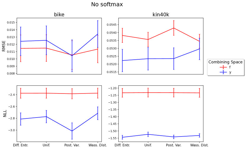
Figure 5: The RMSE and NLL (lower is better) for Deep Vecchia ensemble using different combining methods in both $f$-space (red) and $y$-space (blue) without using the temperature endowed softmax. The left column shows the results on bike and the right columns show the results on kin40k. The vertical bars on each plot repersent one standard deviation (from three repeats). In terms of NLL, combing in $y$-space has better results for every combining method. The results for RMSE are not as clear.

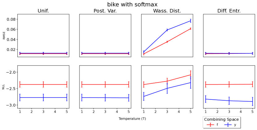
Figure 6: The RMSE and NLL vs temperature (T) for Deep Vecchia ensemble using different combining methods in both $f$-space (red) and $y$-space (blue). The results shown are all for the bike dataset. The vertical bars on each plot represent one standard deviation (from three repeats). It appears that increasing the value of $T$ had meaningful change on the NLL of Wasserstein distance and differential entropy, but not on posterior variance or uniform weighting. For RMSE only Wasserstein distance changed as we varied $T$.

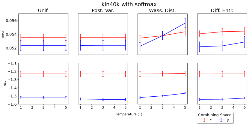
Figure 7: The RMSE and NLL vs temperature (T) for Deep Vecchia ensemble using different combining methods in both $f$-space (red) and $y$-space (blue). The results shown are all for the kin40k dataset. The vertical bars on each plot represent one standard deviation (from three repeats). Just as in Figure 7 NLL changed for Wasserstein distance and differential entropy as we varied $T$, but not for other methods. RMSE for Wasserstein distance and differential entropy were the only two that changed as we increased $T$.

G.3 Choosing a weighting scheme

Table 4 lists four options for computing the weights, $\beta_{k}$, in the row labeled ”Weighting”. Given that we are combining in $y$-space and not using the softmax function, we suggest using the posterior variance in settings similar to ours. The reason being that posterior variance is simple to compute and is among the top performers for both bike and kin40k.

References

- [1] François Bachoc, Louis Béthune, Alberto Gonzalez-Sanz and Jean-Michel Loubes “Gaussian Processes on Distributions based on Regularized Optimal Transport” In International Conference on Artificial Intelligence and Statistics, 2023, pp. 4986–5010 PMLR
- [2] David Bau et al. “Network dissection: Quantifying interpretability of deep visual representations” In Proceedings of the IEEE conference on computer vision and pattern recognition, 2017, pp. 6541–6549
- [3] Yanshuai Cao and David J Fleet “Generalized product of experts for automatic and principled fusion of Gaussian process predictions” In arXiv preprint arXiv:1410.7827, 2014
- [4] Tianqi Chen, Emily Fox and Carlos Guestrin “Stochastic gradient hamiltonian monte carlo” In International conference on machine learning, 2014, pp. 1683–1691 PMLR
- [5] Samuel Cohen, Rendani Mbuvha, Tshilidzi Marwala and Marc Deisenroth “Healing products of Gaussian process experts” In International Conference on Machine Learning, 2020, pp. 2068–2077 PMLR
- [6] Andreas Damianou and Neil D Lawrence “Deep gaussian processes” In Artificial intelligence and statistics, 2013, pp. 207–215 PMLR
- [7] Marc Deisenroth and Jun Wei Ng “Distributed gaussian processes” In International Conference on Machine Learning, 2015, pp. 1481–1490 PMLR
- [8] Yarin Gal and Zoubin Ghahramani “Dropout as a bayesian approximation: Representing model uncertainty in deep learning” In international conference on machine learning, 2016, pp. 1050–1059 PMLR
- [9] Rafael Gómez-Bombarelli et al. “Automatic chemical design using a data-driven continuous representation of molecules” In ACS central science 4.2 ACS Publications, 2018, pp. 268–276
- [10] Antoine Grosnit et al. “High-dimensional Bayesian optimisation with variational autoencoders and deep metric learning” In arXiv preprint arXiv:2106.03609, 2021
- [11] Kaiming He, Xiangyu Zhang, Shaoqing Ren and Jian Sun “Deep residual learning for image recognition” In Proceedings of the IEEE conference on computer vision and pattern recognition, 2016, pp. 770–778
- [12] James Hensman, Nicolo Fusi and Neil D Lawrence “Gaussian processes for big data” In arXiv preprint arXiv:1309.6835, 2013
- [13] Geoffrey E Hinton “Training products of experts by minimizing contrastive divergence” In Neural computation 14.8 MIT Press, 2002, pp. 1771–1800
- [14] Felix Jimenez and Matthias Katzfuss “Scalable bayesian optimization using vecchia approximations of gaussian processes” In International Conference on Artificial Intelligence and Statistics, 2023, pp. 1492–1512 PMLR
- [15] Myeongjong Kang and Matthias Katzfuss “Correlation-based sparse inverse Cholesky factorization for fast Gaussian-process inference” In Statistics and Computing 33.3 Springer, 2023, pp. 56
- [16] Matthias Katzfuss and Joseph Guinness “A General Framework for Vecchia Approximations of Gaussian Processes” In Statistical Science 36.1 Institute of Mathematical Statistics, 2021, pp. 124–141 DOI: 10.1214/19-STS755
- [17] Matthias Katzfuss, Joseph Guinness and Earl Lawrence “Scaled Vecchia approximation for fast computer-model emulation” In SIAM/ASA Journal on Uncertainty Quantification 10.2 SIAM, 2022, pp. 537–554
- [18] Balaji Lakshminarayanan, Alexander Pritzel and Charles Blundell “Simple and scalable predictive uncertainty estimation using deep ensembles” In Advances in neural information processing systems 30, 2017
- [19] Wanhua Li et al. “Bridgenet: A continuity-aware probabilistic network for age estimation” In Proceedings of the IEEE/CVF Conference on Computer Vision and Pattern Recognition, 2019, pp. 1145–1154
- [20] Jeremiah Liu et al. “Simple and principled uncertainty estimation with deterministic deep learning via distance awareness” In Advances in Neural Information Processing Systems 33, 2020, pp. 7498–7512
- [21] Wesley J Maddox et al. “A simple baseline for bayesian uncertainty in deep learning” In Advances in neural information processing systems 32, 2019
- [22] Radford M Neal “Bayesian learning for neural networks” 118, Lecture Notes in Statistics Springer New York, NY, 1996
- [23] Zhenxing Niu et al. “Ordinal regression with multiple output cnn for age estimation” In Proceedings of the IEEE conference on computer vision and pattern recognition, 2016, pp. 4920–4928
- [24] Hongyu Pan, Hu Han, Shiguang Shan and Xilin Chen “Mean-variance loss for deep age estimation from a face” In Proceedings of the IEEE conference on computer vision and pattern recognition, 2018, pp. 5285–5294
- [25] Rasmus Rothe, Radu Timofte and Luc Van Gool “Deep expectation of real and apparent age from a single image without facial landmarks” In International Journal of Computer Vision 126.2 Springer, 2018, pp. 144–157
- [26] Didier Rullière, Nicolas Durrande, François Bachoc and Clément Chevalier “Nested Kriging predictions for datasets with a large number of observations” In Statistics and Computing 28.4 Springer, 2018, pp. 849–867
- [27] Nyeong-Ho Shin, Seon-Ho Lee and Chang-Su Kim “Moving Window Regression: A Novel Approach to Ordinal Regression” In Proceedings of the IEEE/CVF Conference on Computer Vision and Pattern Recognition, 2022, pp. 18760–18769
- [28] Joshua B Tenenbaum, Vin de Silva and John C Langford “A global geometric framework for nonlinear dimensionality reduction” In science 290.5500 American Association for the Advancement of Science, 2000, pp. 2319–2323
- [29] Michalis Titsias “Variational learning of inducing variables in sparse Gaussian processes” In Artificial intelligence and statistics, 2009, pp. 567–574 PMLR
- [30] Volker Tresp “A Bayesian committee machine” In Neural computation 12.11 MIT Press One Rogers Street, Cambridge, MA 02142-1209, USA journals-info …, 2000, pp. 2719–2741
- [31] Aldo V Vecchia “Estimation and model identification for continuous spatial processes” In Journal of the Royal Statistical Society: Series B (Methodological) 50.2 Wiley Online Library, 1988, pp. 297–312
- [32] Andrew Gordon Wilson, Zhiting Hu, Ruslan Salakhutdinov and Eric P Xing “Deep kernel learning” In Artificial intelligence and statistics, 2016, pp. 370–378 PMLR
- [33] Kaipeng Zhang, Zhanpeng Zhang, Zhifeng Li and Yu Qiao “Joint face detection and alignment using multitask cascaded convolutional networks” In IEEE signal processing letters 23.10 IEEE, 2016, pp. 1499–1503
- [34] Zhifei Zhang, Yang Song and Hairong Qi “Age progression/regression by conditional adversarial autoencoder” In Proceedings of the IEEE conference on computer vision and pattern recognition, 2017, pp. 5810–5818