A fermionic path integral for
exact enumeration of polygons on the simple cubic lattice

Abstract

Enumerating polygons on regular lattices is a classic problem in rigorous statistical mechanics. The goal of enumerating polygons on the square lattice via fermionic path integration was achieved using a free-fermion quadratic action in the late 1970s. Given that polygon edges only link 2 vertices, it is considered plausible, if not natural, that an action of degree 2 in the Grassmann variables might suffice to enumerate lattice polygons in any dimension. Nevertheless, on nonplanar lattices the problem has remained open for more than four decades. Here we derive the Grassmann action for exact enumeration of polygons on the simple cubic lattice. Moreover, we prove that this action is not quadratic but quartic — corresponding to a model of interacting fermions.

I Introduction

An important problem in statistical mechanics and enumerative combinatorics concerns how to count certain kinds of objects, such as polygons, polinominoes and polycubes of fixed size, on regular lattices [1]. Here we address the problem of exact enumeration of multipolygons, defined as connected or disconnected undirected graphs whose edges can link only nearest-neighbor lattice sites and all of whose nodes have even degree. A free-fermion quadratic Grassmann action for exact enumeration of 2D multipolygons on the square lattice has been known since the late 1970s [2]. These results were subsequently published by Samuel [3, 4, 5] in 1980 in a seminal trilogy of papers presenting the fermionic path integral formulation of classical lattice spin models. Many advances followed [18, 12, 11, 13, 17, 16, 6, 15, 14, 8, 7, 10, 9], yet for the next 42 years the analogous problem of finding the action for enumerating 3D multipolygons had remained unsolved — until now. Here we derive the Grassmann action for exact enumeration of multipolygons on the simple cubic lattice.

Moreover, considering that an edge connects precisely two vertices of a polygon and assuming that both vertices contribute one Grassmann variable each to the edge terms of the action, it follows that a quadratic Grassmann action should suffice for polygon enumeration not only in two dimensions but in any lattice dimension. The underlying intuition is rooted in familiar commonplace observations, for example if one wishes to string together a bead necklace, it suffices to make 2 holes per bead. Indeed, it is often assumed that polygons on the cubic lattice should be enumerable with a quadratic action. This conjecture, though plausible, turns out to be wrong. Overturning the conventional wisdom, we prove that the action that enumerates polygons on the simple cubic lattice is not quadratic but quartic — hence unsolvable via existing methods that rely on the usual pfaffian methods that apply to quadratic actions. We also show that, quite remarkably, the action for the cubic lattice is not polynomial in the edge weights.

Our strategy is to exploit how the ferromagnetic 3D Ising model can be formulated in two different ways. On the one hand, it can be formulated in a low temperature variable in terms of the generating function of closed surfaces on the simple cubic lattice [5]. On the other hand, it is also possible to formulate the model in a high temperature variable in terms of the generating function of multipolygons. The latter approach is more commonly used in statistical mechanics [19, 20, 21, 22]. We leverage the known [22] exact correspondence between the two formulations and “work backwards,” thereby obtaining the desired Grassmann action.

The high and low temperature formulations of the Ising model are reviewed in Sec. II. A review of Grassmann variables and Berezin integration is given in Sec. III. This section also gives a detailed explanation of the Grassmann actions for the 2D and 3D Ising model. Sec. IV presents the results and advances and Sec. V concludes with a brief discussion.

II The high and low temperature formulations of the 3D Ising model.

The Hamiltonian of the isotropic ferromagnetic Ising model with $N$ classical spins with nearest-neighbor interactions and zero external magnetic field is typically defined as $H_{N}=-J\sum_{\mbox{$\left\langle\,{ij}\,\right\rangle$}}\sigma_{i}\sigma_{j}$ where the $J$ is the isotropic coupling, $\sigma_{i}=\pm 1$ and $\left\langle\,{ij}\,\right\rangle$ denotes the set of all pairs $(i,j)$ of nearest-neighbor spins on the chosen lattice. The total number of sites is $N=L^{d}$ for a system of linear size $L$ on a $d$-dimensional grid lattice. In what follows we restrict our attention to the cases $d=2,3$ for the square and simple cubic lattices respectively. Although diverse boundary conditions can be used, we assume periodic boundary conditions without loss of generality. Indeed, it is well known that the thermodynamic limit of the nearest-neighbor Ising model is independent of boundary conditions. The canonical partition function is conventionally defined according to $Z_{N}(\beta)=\sum\exp[-\beta H_{N}]$, where $\beta=1/(k_{\mbox{\tiny B}}T)$ is the temperature parameter as usual and the sum is over all possible spin configurations.

Let $K=\beta J$ be the (adimensional) reduced temperature parameter. For studying the behavior at low temperatures (i.e. high $\beta$), by convention [3, 23] one uses the low temperature variable $u=\exp[-K]$ (although sometimes the square or fourth power of this quantity is used instead [22]). On the other hand, for studying the high temperature behavior of the model it is often preferable [19, 20, 21, 22] to use the high temperature variable $t=\tanh[K]$. For non-negative reduced temperatures $0\leq K\leq+\infty$, the low and high temperature variables are uniquely given by each other, according to

$$u ={\sqrt{1-t\over 1+t}}$$

$$t ={1-u^{2}\over 1+u^{2}}\leavevmode\nobreak\ .$$

In the high temperature variable $t$, it is well known [19] that the partition function can be expressed as

$$Z_{N}=2^{N}(1-t^{2})^{-Nd/2}\Lambda_{N}(t)\leavevmode\nobreak\ ,$$ (1)

where $\Lambda(t)$ is the generating function for the number of multipolygons of fixed length on the $d$-dimensional lattice. Specifically, if we write $\Lambda_{N}$ as the expansion

$$\Lambda_{N}(t)=\sum_{n=0}^{Nd}a_{n}t^{n}\leavevmode\nobreak\ ,$$

then $a_{n}$ is the number of multipolygons with $n$ edges, with the total number of all edges being $Nd$. Note that $a_{0}=1$, corresponding to the single empty graph. For clarity we repeat here the textbook derivation of the Eq. (1). First observe that $\sigma_{i}\sigma_{j}=\pm 1$, so that $\exp[-\beta H_{N}]$ is given by

$$\exp\left[K\textstyle\sum\sigma_{i}\sigma_{j}\right] =\prod\exp[K\sigma_{i}\sigma_{j}]$$

$$=\prod\cosh K+\sigma_{i}\sigma_{j}\sinh K$$

$$=\prod(\cosh K)(1+\sigma_{i}\sigma_{j}t)\leavevmode\nobreak\ .$$ (2)

Noting that $\cosh K=1/\sqrt{1-t^{2}}$ and that the total number of terms in the product is equal to the number $Nd$ of bonds, we can write the partition function as

$$Z_{N}=(1-t^{2})^{-Nd/2}\sum_{\sigma_{1}}\sum_{\sigma_{2}}\cdots\sum_{\sigma_{N}}\prod_{\small\mbox{$\left\langle\,{ij}\,\right\rangle$}}(1+\sigma_{i}\sigma_{j}t)\leavevmode\nobreak\ .$$ (3)

Each $\sigma_{i}$ is summed over $\pm 1$, so the only terms that survive upon expanding the product are those with no odd powers of any of the $\sigma_{i}$. Remaining even powers $\sigma_{i}^{2n}$ contribute a factor $1^{2n}+(-1)^{2n}=2$ for each of the $N$ sites. The product is over all possible nearest-neighbor “bonds,” hence

$$Z_{N}=2^{N}(1-t^{2})^{-Nd/2}\sum_{G\in\mathcal{M}}t^{m(G)}\leavevmode\nobreak\ ,$$ (4)

where $m(G)$ is the number of edges of the graph $G$ and $\mathcal{M}$ is the set of all undirected unweighted graphs on the lattice whose edges only link nearest-neighbor nodes and whose nodes all have even degree, with the unique empty graph having $m=0$. Eq. (1) follows from (4) by observing that these graphs $G\in\mathcal{M}$ are precisely what we have been calling multipolygons. Feynman [19] referred to multipolygons as “closed graphs” due to the fact that there are no dangling edges or common sides, i.e. no nodes of degree 1 or 3. In 3D such multipolygons need not be planar.

Alternatively, we can express the partition function in terms of the low temperature variable $u$, by counting the number of magnetic domain wall configurations. Let $\Xi(u)$ be the generating function for the number of domain wall configurations of fixed size [23]. In 2D this will again correspond to the number of multipolygons of fixed length (because the 2D Ising model is self-dual). In contrast, in 3D magnetic domain walls are closed surfaces on the dual lattice. Specifically, if we write the expansion

$$\Xi_{N}(u)=\sum_{n=0}^{Nd}b_{n}u^{2n}\leavevmode\nobreak\ ,$$

then $b_{n}$ is the number of domain wall configurations of length $n$ (2D) or area $n$ (3D). Taking into account the ground state energy $-NdJ$, and a factor $2$ arising from the twofold degeneracy associated with each domain wall configuration, the partition function is then given in terms of $\Xi_{N}$, as is well known [23]:

$$Z_{N}=2u^{-Nd}\leavevmode\nobreak\ \Xi_{N}(u)\leavevmode\nobreak\ .$$ (5)

Per-site partition function and the other generating functions in the thermodynamic limit $N\to\infty$ are defined as usual according to $Z=\lim_{N\to\infty}Z_{N}^{1/N}$, $\Lambda=\lim_{N\to\infty}\Lambda_{N}^{1/N}$ and $\Xi=\lim_{N\to\infty}\Xi_{N}^{1/N}$.

Crucially, given $\Xi_{N}$ one can obtain $\Lambda_{N}$ (and v.v.):

$$\Lambda_{N}(t) =2^{1-N}(1-t^{2})^{Nd/2}u^{-Nd}\leavevmode\nobreak\ \Xi_{N}(u)$$

$$=2^{1-N}(1+t)^{Nd}\leavevmode\nobreak\ \Xi_{N}\left(\sqrt{1-t\over 1+t}\right)\leavevmode\nobreak\ .$$ (6)

In 2D, both $\Xi$ and $\Lambda$ are explicitly known because of Onsager’s solution [24]. But in 3D neither $\Xi$ nor $\Lambda$ is explicitly known. However, there are partial results in 3D. The fermionic path integral for $\Xi$ has been known [5] since 1980. In contrast, until now no analogous expression for $\Lambda$ has been known. Our main contribution here is to obtain the fermionic path integral for $\Lambda$ for the simple cubic lattice, by using (6).

III The Grassmann action for the Ising model

III.1 Grassmann variables and Berezin integration

The fermionic aspect of the 2D Ising model was already implicitly apparent in the original works of Onsager and of Kaufmann, as seen from their use of quaternion algebra [24] and generators of the Pauli spin matrices [25]. A few decades later, in 1964, Schultz, Mattis and Lieb formally showed that the 2D Ising model is equivalent to a free-fermion model [26], by employing fermionic creation and annihilation operators satisfying canonical anticommutation relations. It was only in 1980 that the much more powerful fermionic path integral formulation of the 2D Ising model was given [3] in terms of Grassmann variables, i.e. fully anticommuting quantities.

Let $\eta_{i}\leavevmode\nobreak\ (i=1,2,\ldots,N)$ be a set of Grassmann numbers that satisfy

$$\eta_{i}\eta_{j}+\eta_{j}\eta_{i}=0\leavevmode\nobreak\ .$$ (7)

In particular, such quantities are nilpotent, $\eta_{i}^{2}=0$. A general power series in these $N$ quantities, with real or complex coefficients, can thus only have $2^{N}$ terms at most, so that the Grassmann algebra thus generated has dimension $2^{N}$. Integrals of Grassmann variables are known as Berezin integrals, in honor of Felix Berezin [27], who showed how to modify Feynman’s (bosonic) path integrals to be applicable to fermions. Berezin integration is a translationally invariant linear operation defined (in the standard convention used in physics) according to

$$\displaystyle\int\eta_{i}d\eta_{i} \leavevmode\nobreak\ =\leavevmode\nobreak\ 1\leavevmode\nobreak\ ,$$ (8)

$$\displaystyle\int d\eta_{i}\quad \leavevmode\nobreak\ =\leavevmode\nobreak\ 0\leavevmode\nobreak\ .$$ (9)

Multiple integrals can be defined as iterated integrals. Let $d\eta$ be shorthand for $d\eta_{1}d\eta_{2}\ldots d\eta_{N}$ and $\eta$ for the entire set $\{\eta_{1},\eta_{2},\ldots,\eta_{N}\}$. Consider a general function

$$f(\eta) =a_{0}+\sum_{i}^{N}a_{i}\eta_{i}+\sum_{i<j}^{N}a_{ij}\eta_{i}\eta_{j}$$

$$\quad\quad+\cdots+a_{123\ldots N}\eta_{1}\eta_{2}\cdots\eta_{N}\leavevmode\nobreak\ .$$ (10)

Then from the definition of Berezin integration we find

$$\int f(\eta)d\eta=a_{123\ldots N}\leavevmode\nobreak\ .$$ (11)

Hence, Berezin integrals can be used retain only those terms that “saturate” the integral. Using the Lagrangian path integral formulation of Hamiltonian systems, a Berezin integral $\int e^{S}d\eta$ of an exponentiated Grassmann action $S$ can be used to select states with specific properties, rendering it an extremely powerful tool in exact enumeration problems.

We will also require the use of a key property of how Berezin integrals transform under changes of variables. For usual Riemann integrals $\int f(x)dx$ over, say, the reals $\mathbb{R}$, a change of variables $x=ay$ with $a\in\mathbb{R}$ leads to $dx=ady$ for the differentials. However, for Grassmann variables $x$ and $y$, if $x=ay$ with $a\in\mathbb{R}$, then $dx=dy/a$ because of (8). In other words, the scaling is in the opposite sense. Let us apply such scale transformations to the actions, considered as functionals of the $\eta$. Let $q$ Grassmann variables reside at each of $N$ lattice sites. Consider the result of the dilation $\eta_{i}\mapsto\lambda\eta_{i}$, for all $qN$ Grassmann variables. Let $\eta^{\prime}=\lambda\eta$ be the rescaled variables. Then applying the rule for changing Grassmann variables, we obtain $\int d\eta\leavevmode\nobreak\ e^{S(\eta)}=\int d\eta^{\prime}\leavevmode\nobreak\ e^{S[\eta^{\prime}]}=\lambda^{-qN}\int d\eta\leavevmode\nobreak\ e^{S[\lambda\eta]}$. Taking the $qN$-th root of $\lambda$ we thus get

$$\lambda\int d\eta\leavevmode\nobreak\ e^{S(\eta)}=\int d\eta\leavevmode\nobreak\ e^{S[\lambda^{1/qN}\eta]}\leavevmode\nobreak\ .$$ (12)

This renormalization of the Grassmann variables will play a central role in the derivation below of the exact Grassmann action for 3D multipolygons.

III.2 2D multipolygons

The original work of Samuel [3] included a remarkable “one line” solution of the 2D Ising model, leading immediately to Onsager’s solution [24] in less than a “a page of algebra” [3]. The generating function for 2D multipolygons, whose coefficients are the celebrated series found by Cyril Domb, also easily follows (see also ref. [28]). In notation similar to that of ref. [23], the action for the isotropic model can be written as

$$S_{2D}(\eta) =u^{2}S_{L}(\eta)+S_{C}(\eta)+S_{M}(\eta)\leavevmode\nobreak\ ,$$ (13)

$$S_{L}(\eta) =\sum_{x\in\mathcal{L}}^{N}\bigg{[}\eta_{+1}(x)\eta_{-1}(x+\hat{1})$$

$$\quad\quad\quad\quad+\eta_{+2}(x)\eta_{-2}(x+\hat{2})\bigg{]}\leavevmode\nobreak\ ,$$ (14)

$$S_{M}(\eta) =\sum_{x\in\mathcal{L}}^{N}(\eta_{-1}(x)\eta_{+1}(x)+\eta_{-2}(x)\eta_{+2}(x))\leavevmode\nobreak\ ,$$ (15)

$$S_{C}(\eta) =\sum_{x\in\mathcal{L}}^{N}\bigg{[}\eta_{+1}(x)\eta_{-2}(x)+\eta_{+2}(x)\eta_{-1}(x)$$

$$\quad\quad\quad\quad+\eta_{+2}(x)\eta_{+1}(x)+\eta_{-2}(x)\eta_{-1}(x)\bigg{]}\leavevmode\nobreak\ .$$ (16)

The sums are over all sites of the dual lattice $\mathcal{L}$ of the magnetic domain walls. The subscripts $M$, $L$, and $C$ denote monomers, lines and corners [23]. Each line term is associated with a single edge with weight $u^{2}$ of a single segment of domain wall. It can be checked by manual Berezin integration, for any given configuration of lines, monomers and corners, that sites attached to 1 or 3 lines give zero contribution, making the full Berezin integral vanish. Sites with 2 and 4 attached line terms contribute with a factor $u^{2}$ for each line. Sites with no lines contribute $-1$ but such sites can only ever appear in pairs, so for even $N$ the factor can be neglected.

The Berezin integral of the (exponentiated) action (13) thus enumerates multipolygons on the square lattice, thereby counting all possible magnetic domain wall configurations of the 2D Ising model. Hence,

$$\Xi(u)=(-1)^{N}\int\prod^{N}_{x\in\mathcal{L}}d\eta_{-1}d\eta_{+1}d\eta_{-2}d\eta_{+2}\exp[S_{2D}]\leavevmode\nobreak\ .$$ (17)

We will write such expressions more compactly as

$$\Xi(u)=(-1)^{N}\int d\eta\exp[S_{2D}]\leavevmode\nobreak\ .$$ (18)

The partition function is then given by (5). In the literature the factor $(-1)^{N}$ is usually omitted because $N$ can be taken as even and, moreover, it can be neglected in general when taking the thermodynamic limit since $\lim_{N\to\infty}(-1)^{1/N}=1$, but we retain the sign for completeness. Fourier transformation and the application of the well known determinant formula for Gaussian integrals immediately leads [3] to Onsager’s solution (not shown here, see Eq. (3.12) in ref. [3]).

III.3 The action for the 3D Ising model

In 1980 Samuel also wrote down the analogous Grassmann action for the 3D Ising model [5]. However, this action enumerates not multipolygons but rather closed surfaces. Let $\eta$ denote the set of $12N$ Grassmann variables $\eta_{\pm\nu}(x,\mu)$ following the notation of ref. [23], where $x$ is the site index as before and $\mu$ is the edge index, with $\pm\nu$ describing the side of the edge where the variable resides. See Figure 1 for the arrangement of the Grassmann variables. Then the action for the isotropic Ising model can be written as

$$S_{3D}(\eta,u)=u^{2}\leavevmode\nobreak\ S_{4}(\eta)+S_{2}(\eta)\leavevmode\nobreak\ ,$$ (19)

where

$$\leavevmode\nobreak\ \leavevmode\nobreak\ S_{4}(\eta) =\sum_{x}^{N}\bigg{\{}$$

$$\begin{array}[t]{l}\leavevmode\nobreak\ \leavevmode\nobreak\ \leavevmode\nobreak\ \eta_{+2}(x,3)\eta_{-2}(x+\hat{2},3)\eta_{+3}(x,2)\eta_{-3}(x+\hat{3},2)\\ +\leavevmode\nobreak\ \eta_{+1}(x,3)\eta_{-1}(x+\hat{1},3)\eta_{+3}(x,1)\eta_{-3}(x+\hat{3},1)\\ +\leavevmode\nobreak\ \eta_{+1}(x,2)\eta_{-1}(x+\hat{1},2)\eta_{+2}(x,1)\eta_{-2}(x+\hat{2},1)\bigg{\}}\leavevmode\nobreak\ ,\end{array}\vspace{-2cm}\leavevmode\nobreak\$$ (23)

$$S_{2}(\eta) =\sum_{x}^{N}\sum_{\mu=1}^{3}\sum_{\begin{subarray}{c}\leavevmode\nobreak\ \nu,\rho\neq\mu\\ \nu<\rho\end{subarray}}^{3}\bigg{\{}\begin{array}[t]{l}\displaystyle\leavevmode\nobreak\ \leavevmode\nobreak\ \leavevmode\nobreak\ \eta_{+\nu}(x,\mu)\leavevmode\nobreak\ \eta_{-\rho}(x,\mu)\\ +\leavevmode\nobreak\ \eta_{+\rho}(x,\mu)\leavevmode\nobreak\ \eta_{+\nu}(x,\mu)\\ +\leavevmode\nobreak\ \eta_{+\rho}(x,\mu)\leavevmode\nobreak\ \eta_{-\nu}(x,\mu)\\ +\leavevmode\nobreak\ \eta_{-\rho}(x,\mu)\leavevmode\nobreak\ \eta_{-\nu}(x,\mu)\\ +\leavevmode\nobreak\ \eta_{-\nu}(x,\mu)\leavevmode\nobreak\ \eta_{+\nu}(x,\mu)\\ +\leavevmode\nobreak\ \eta_{-\rho}(x,\mu)\leavevmode\nobreak\ \eta_{+\rho}(x,\mu)\leavevmode\nobreak\ \bigg{\}}\leavevmode\nobreak\ .\nobreak\leavevmode\end{array}$$ (30)

The quartic “plaquette” terms $u^{2}S_{4}$ and the quadratic “hinge” terms $S_{2}$ above correspond to the terms $S_{P}(\eta)$ and $S_{E}(\eta)+S_{M}(\eta)$, respectively, in ref. [23].

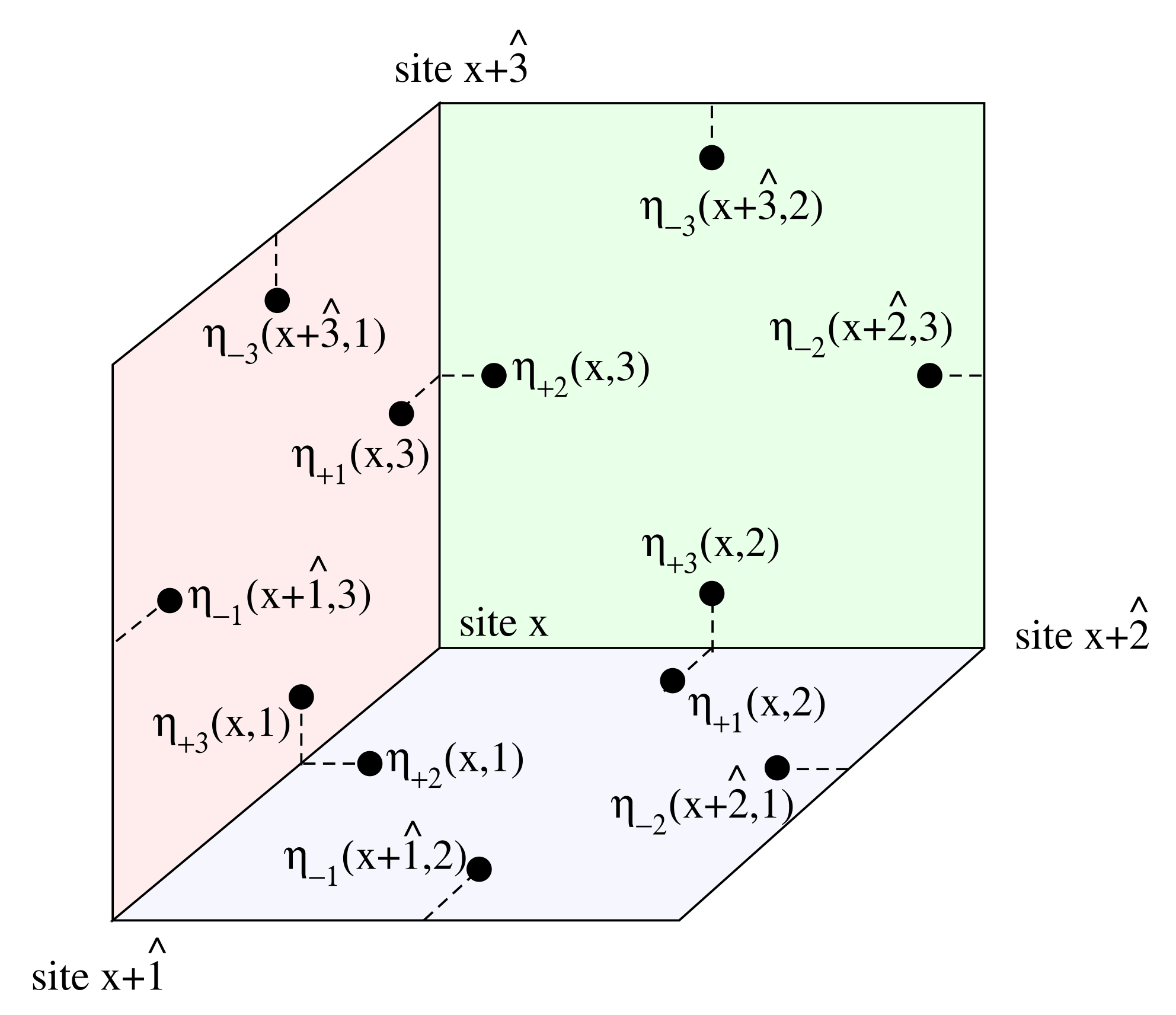
Figure 1: Arrangement of the Grassmann variables on the (dual) simple cubic lattice. The variables $\eta_{\pm\nu}(x,\mu)$ are indexed by the position $x$, by the type of edge $\mu$, and by positive or negative directions $\pm\nu$. The 3 primitive translation vectors are denoted $\widehat{1}$, $\widehat{2}$ and $\widehat{3}$. For a different perspective of the same arrangement, see Figure 6 of ref. [23].

As with the 2D action, it is easy to see that this action enumerates closed surfaces, as follows. Edges with 1 or 3 attached plaquettes give contribution zero and render the full Berezin integral zero. Edges with 2 or 4 attached plaquettes contribute with a factor $u^{2}$ for each plaquette. Edges with no plaquette give a factor of $-1$. Let $d\eta$ be shorthand according to

$$d\eta=\prod_{x}^{N}\prod_{\mu=1}^{3}\prod_{\nu\neq\mu}^{3}d\eta_{-\nu}(x,\mu)d\eta_{+\nu}(x,\mu)\leavevmode\nobreak\ .$$

Then the partition function is given by (5) with

$$\Xi_{N}(u)=(-1)^{3N}\int d\eta\exp[S_{3D}]\leavevmode\nobreak\ .$$ (32)

Since this action is not quadratic, it does not correspond to a model of free fermions, but rather to a model of interacting fermions. Moreover, pfaffian and determinant formulas cannot be used in the usual manner because the integrals are not Gaussian. Nevertheless, over the decades significant progress been made even without being able to obtain explicit expressions and the Grassmannization research program has, overall, been tremendously successful  [18, 12, 11, 13, 17, 16, 6, 15, 14, 8, 7, 10, 9].

IV The quartic action for enumerating 3D multipolygons

We now present our main results. In what follows, we will use the action (19) as a the starting point to arrive at the analogous action for counting multipolygons on the simple cubic lattice. Substituting (32) into (6) we get

$$\Lambda_{N}(t)=2^{1-N}(1+t)^{3N}\leavevmode\nobreak\ (-1)^{3N}\int d\eta\leavevmode\nobreak\ e^{S_{3D}(\eta,u)}\leavevmode\nobreak\ .$$ (33)

Applying the rescaling (12) to (33) we arrive at our first result:

$$\Lambda_{N}(t)=(-1)^{3N}\int d\eta\leavevmode\nobreak\ e^{S_{3D}[2^{1/(12N)-1/12}(1+t)^{1/4}\eta,u]]}\leavevmode\nobreak\ .$$

Let $S_{3DM}$ denote the Grassmann action for exact enumeration of multipolygons on the simple cubic lattice. Then the above result can be written

$$\Lambda_{N}(t) =(-1)^{3N}\int d\eta\exp[{S_{3DM}}]$$ (34)

$$S_{3DM}(\eta,t) ={S_{3D}(2^{1/(12N)-1/12}(1+t)^{1/4}\eta,u)}\leavevmode\nobreak\ .$$ (35)

Of particular interest in statistical mechanics are the thermodynamic limits of various quantities, such as partition functions and generating functions. Using (19) and taking the limit $N\to\infty$, the (35) simplifies to

$$S_{3DM}(\eta,t) =\frac{(1+t)^{1/2}}{\sqrt[6]{2}}S_{2}(\eta)+\frac{(1-t)}{\sqrt[3]{2}}S_{4}(\eta)\leavevmode\nobreak\ ,$$ (36)

with $S_{2}$ and $S_{4}$ given by (LABEL:eq-Sh ) and (23) respectively.

Finally, the claim that $S_{3DM}$ in (36) is quartic follows immediately from observing that $S_{4}$ by definition (23) is quartic in the Grassmann variables. Whereas quadratic actions correspond to free fermion models, quartic actions are associated with (typically unsolved) models of interacting fermions. The known singularity at $t=t_{c}$ of $\Lambda(t)$ for the simple cubic lattice bears an important relation to string and gauge field theories [9]. Indeed, it is possible to represent the continuum limit of the 3D Ising model in terms of a fermion string theory [29, 30, 31].

Note that $S_{3DM}$ is not polynomial in the edge weight $t$, because Eq. (36) contains a square root term that leads to a non-terminating binomial power series in $t$. Hence, on the cubic lattice there are no well defined polynomial “edge terms” in the action, in contrast to the action $S_{2D}$ for the square lattice, which has the edge terms $S_{L}$ in (13). Planar and nonplanar polygons are very different indeed.

Nevertheless, note that upon expansion of the corresponding exponential and subsequent saturation of the Berezin integral, all surviving terms have an even number of quadratic terms contributing, such that the square root completely vanishes and the dependence on $t$ is again polynomial. Indeed, every plaquette contributes $(1-t)/\sqrt[3]{2}$ and every “missing plaquette” contributes precisely $(1+t)/\sqrt[3]{2}$ in the thermodyamic limit.

V Discussion and Conclusion

In summary, we have solved the 42-year-old problem of finding the Grassmann action for exact enumeration of polygons on the simple cubic lattice. The Grassmann action for enumerating multipolygons on the cubic lattice is quartic, not quadratic, and has a remarkable non-polynomial dependence on the edge weight $t$. The significance of these results is that, on the simple cubic lattice, enumerating multipolygons is of the same order of difficulty as enumerating closed surfaces — not easier.

Nevertheless, it should be emphasized that there is no reason at all to expect this action to be unique. In the 2D case it is possible to give a constructive proof of this non-uniqueness, using the pfaffian or determinant formulas for the Gaussian integrals. In the 3D case the question is not so clear. Absent a mathematical proof, we cannot in principle completely rule out the existence of a different — possibly even quadratic — action that performs the same enumeration, however unlikely this may seem. These and similar issues merit further investigation.

Finally, we note that the results presented here suggest that Grassmann actions can be found for polygon enumeration on diverse other regular lattices. We have preliminary results generalizing the above results to other nonplanar lattices, which we hope to publish when time permits.

References

- [1] A. J. Guttmann (Ed.) Polygons, Polyominoes and Polycubes (Springer, Dordrecht, 2009).
- [2] S. Samuel, The Use of Anticommuting Integrals in Statistical Mechanics I. Lawrence Berkeley National Laboratory. LBNL Report #: LBL-8217 (1978).
- [3] S. Samuel, The use of anticommuting variable integrals in statistical mechanics. I. The computation of partition functions, J. Math. Phys. 21, 2806–2814 (1980).
- [4] S. Samuel, The use of anticommuting variable integrals in statistical mechanics. II. The computation of correlation functions, J. Math. Phys. 21, 2815–2819 (1980).
- [5] S. Samuel, The use of anticommuting variable integrals in statistical mechanics. III. Unsolved models”, J. Math. Phys. 21, 2820–2833 (1980).
- [6] Ising fermions (II). Three dimensions, C. Itzykson, Nucl. Phys. B 210, 477 (1982).
- [7] V. N. Plechko, Simple solution of two-dimensional Ising model on a torus in terms of Grassmann integrals, Theor Math Phys 64, 748 (1985).
- [8] R. Shankar, Exact critical-behavior of a random-bond two-dimensional Ising-model, Phys. Rev. Lett., 58, 2466 (1987).
- [9] A. M. Polyakov, Gauge Fields and Strings (Harwood Academic Publishers, London, 1987).
- [10] C. Itzykson J. M. and Drouffe Statistical Field Theory. Vol 1 (Cambridge, Cambridge University Press,1991).
- [11] F. Mila, Low-energy sector of the Kagome antiferromagnet, Phys. Rev. Lett., 81, 2356 (1998).
- [12] R. Moessner, S. L. Sondhi, Resonating valence bond phase in the triangular lattice quantum dimer model, Phys. Rev. Lett. 86, 1881 (2001).
- [13] F. Ardonne, P. Fendley, E. Fradkin, Topological order and conformal quantum critical points, Annals of Phys. 310, 493 (2004).
- [14] L. Pollet, M. N. Kiselev, N. V. Prokof’ev, B. V. Svistunov, Grassmannization of classical models, New J. Phys. 18, 113025 (2016).
- [15] A. Smerald, F. Mila, Spin-liquid behaviour and the interplay between Pokrovsky-Talapov and Ising criticality in the distorted, triangular-lattice, dipolar Ising antiferromagnet, SciPost Phys 5, 30 (2018).
- [16] B. Dittrich, C. Goeller, E. R. Livine, A. Riello, Quasi-local holographic dualities in non-perturbative 3d quantum gravity I - Convergence of multiple approaches and examples of Ponzano-Regge statistical duals, Nucl. Phys. B 938, 807 (2019).
- [17] N. Matsumoto, K. Kawabata, Y. Ashida, S. Furukawa, M. Ueda Continuous Phase Transition without Gap Closing in Non-Hermitian Quantum Many-Body Systems, Phys. Rev. Lett. 125, 260601 (2020).
- [18] S. Balasubramanian, V. Galitski, A. Vishwanath, Classical vertex model dualities in a family of two-dimensional frustrated quantum antiferromagnets, Phys. Rev. B 106, (2022).
- [19] R. P. Feynman, Statistical Mechanics: A Set Of Lectures (CRC Press, Boca Raton, 1998).
- [20] B. M. McCoy and T. T. Wu, The Two-Dimensional Ising Model (Cambrigde, Harvard, 1973).
- [21] D. Hansel, J. M. Maillard, J. Oitmaa, and M. J. Velgakis, Analytical properties of the anisotropic cubic Ising model, J. Stat. Phys. 48, 69-80 (1987).
- [22] A. J. Guttmann and I. G. Enting, Series studies of the Potts model. I: The simple cubic Ising model, J. Phys. A 26, 807-822 (1993).
- [23] C. R. Gattringer, S. Jaimungal, G. W. Semenoff, Loops, surfaces and Grassmann representation in two- and three- dimensional Ising models, Int. J. Mod. Phys. A 14, 4549-4574 (1999).
- [24] L. Onsager, Crystal Statistics. I. A Two-Dimensional Model with an Order-Disorder Transition Phys. Rev. 65, 117 (1944).
- [25] B. Kaufman, Crystal Statistics. II. Partition Function Evaluated by Spinor Analysis, Phys. Rev. 76, 1232 (1949).
- [26] T. D. Schultz, D. C. Mattis and E. H. Lieb, Two-Dimensional Ising Model as a Soluble Problem of Many Fermions, Rev. Mod. Phys. 36, 856 (1964).
- [27] F. A. Berazin, The Method of Second Quantization (Academic Press, 1966).
- [28] G. M. Viswanathan, The double hypergeometric series for the partition function of the 2D anisotropic Ising model, J. Stat. Mech. 2021 073104 (2021).
- [29] A. M. Polyakov, String representations and hidden symmetries for gauge fields, Phys. Lett. B 82, 247 (1979).
- [30] Vl. S. Dotsenko, 3D Ising model as a free fermion string theory: An approach to the thermal critical index calculation, Nucl. Phys. B 285, 45 (1987).
- [31] Vl. S. Dotsenko and A.M. Polyakov, Fermion representations for the 2D and 3D Ising models, in Conformal Field Theory and Solvable Lattice Models, Eds. M. Jimbo, T. Miwa, A. Tsuchiya (Academic press, 1988).