Explaining Deep Learning for ECG Analysis: Building Blocks for Auditing and Knowledge Discovery

Abstract

Deep neural networks have become increasingly popular for analyzing ECG data because of their ability to accurately identify cardiac conditions and hidden clinical factors. However, the lack of transparency due to the black box nature of these models is a common concern. To address this issue, explainable AI (XAI) methods can be employed. In this study, we present a comprehensive analysis of post-hoc XAI methods, investigating the local (attributions per sample) and global (based on domain expert concepts) perspectives. We have established a set of sanity checks to identify sensible attribution methods, and we provide quantitative evidence in accordance with expert rules. This dataset-wide analysis goes beyond anecdotal evidence by aggregating data across patient subgroups. Furthermore, we demonstrate how these XAI techniques can be utilized for knowledge discovery, such as identifying subtypes of myocardial infarction. We believe that these proposed methods can serve as building blocks for a complementary assessment of the internal validity during a certification process, as well as for knowledge discovery in the field of ECG analysis.

1 Introduction

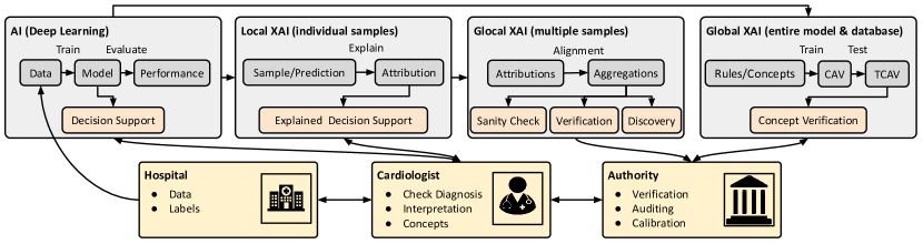
Figure 1: Overview of different XAI approaches proposed in the context of ECG analysis along with corresponding applications (orange boxes). A deep learning model is trained on ECG data, which is supposed to be used as a decision support system. Local XAI methods allow the extraction of per-sample attribution maps for this model, which can be used as side information for practitioners. We propose sanity checks to identify XAI methods that behave reliably. Under the name of glocal XAI, we introduce attribution maps aggregated over entire subgroups of patients, which can be used for auditing as well as knowledge discovery. Finally, we propose to use global XAI methods to verify if expert concepts are exploited by the model, which can serve as a complementary auditing component to assess the internal consistency of the model.

The electrocardiogram (ECG) is one of the most frequently performed diagnostic procedures [1] and plays a unique role in the first-in-line assessment of a patient’s cardiac state. Until this day, most ECGs are assessed manually with only limited support through rule-based algorithms implemented in ECG devices subject to well-known limitations [2]. In the last few years, this analysis paradigm has started to change drastically as a consequence of evidence from an increasing number of studies, which demonstrate the enormous diagnostic potential of the ECG in combination with modern deep learning methods, see [3] for a recent perspective. Most remarkably, this does not only apply to the prediction of diagnostic statements as routinely assessed also by cardiologists, from myocardial infarctions [4] over comprehensive prediction of ECG statements [5, 6], and rhythm abnormalities [7] to challenging conditions such as hypertrophic cardiomyopathy [8], but includes conditions that are hard or even impossible to infer from an ECG for human experts. For example, a number of recent works demonstrated the ability to infer age and sex [9], ejection fraction [10], atrial fibrillation during sinus rhythm [11], anemia [12] or even non-cardiac conditions such as diabetes [13] or cirrhosis [14]. These very promising findings will eventually transform the role the ECG plays in routine diagnostics with enormous potential for cost savings and improved patient journeys through more precise decisions for follow-up diagnostics or treatments.

Modern deep learning models owe their superior performance to their large number of millions to billions of parameters, which allow to capture complicated combinations of input features. However, this flexibility comes at the price of the impossibility to interpret such models on a parameter basis, which is why these are often perceived as black boxes. This led to the emergence of explainable AI (XAI) as a subfield of machine learning, which tries to shed light on the decision process implemented by neural networks, see [15, 16, 17, 18] for general reviews. Here it is important to keep in mind that different use cases pose different requirements for the combined ML+XAI system (see Fig. 1 for an overview). These range from (1) Providing side-information to medical experts (2) Auditing of the ML system before deployment, e.g., to ensure that the models avoid excessive exploitation of spurious correlations or rely on undesired features/principles, see [19] for a recent application (3) Scientific discovery through using the ML model as a proxy for the relations between input and output in the data. While the first use-case is very important, it can eventually only be assessed within user studies. In this work, we focus primarily on the last two aspects and provide building blocks that can be employed in these contexts. Both topics relate to the frequent question of the alignment of neural network decisions and cardiologists’ decision rules, which is rarely assessed systematically beyond single hand-picked examples. At this point, we present two methods that provide quantitative evidence of whether a neural network systematically exploits specific decision rules and which segments of the signal are most relevant for the classification decision across all samples with a particular pathology across an entire dataset. In both cases, we find good agreement across a diverse set of four pathologies.

Various XAI methods have been applied to deep learning models trained on ECG data, see [20] for a recent review, mostly in the form of ad-hoc adaptations of existing methods mostly from computer vision. With very exceptions, such as [21] or [22], who relied on model-inherent attention weights, most approaches involved so-called post-hoc XAI methods applied to trained models. The clearly most popular approach considered in the ECG literature is GradCAM [23], used for example by [24, 12, 25, 26, 27, 28]. GradCAM is followed in popularity by saliency maps [29], see [30, 31, 32, 33]. Other choices include LIME [34]. These techniques provide visually appealing attribution maps that are in most cases used to argue whether the decision criteria of deep neural networks align with human expert knowledge.

However, prior approaches rarely provided arguments why a particular XAI method was chosen or if it was appropriate for this purpose. We argue that the ECG is particularly suited for a structured evaluation due to its periodic structure and ECG features as well-defined signal features. This makes it possible to set up precise sanity checks for XAI methods, allowing you to assess whether they attribute consistently, both in a temporal as well as spatial manner. As one exemplary finding, we demonstrate that most existing approaches including GradCAM with the exception of saliency maps, fail to attribute in a temporally focused manner, which clearly puts into question existing approaches in the field.

As second contribution, we aim to stress opportunities for XAI methods beyond attribution maps. To this end, we apply TCAV [35], which allows to assess if a model uses a given concept, defined via examples. Again, we argue that the ECG domain represents an ideal application domain for such techniques due to the availability of high-quality ECG features and concepts as defined via cardiologists’ decision rules, and demonstrate potential application for auditing ML models in the ECG domain.

As third main contribution, we strongly argue for the automated analysis of attributions in a beat-aggregated form, in line with earlier proposals in the literature [31, 25, 36]. We exploit the periodic structure of the signal to provide attribution maps on the level of median beats. These can be compared in a meaningful way across samples and patients. In this way, attribution maps can be aggregated across patients (with similar pathologies) to derive dataset-wide patterns from sample-specific attribution maps. We showcase this approach for three major diagnostic classes.

Finally, we demonstrate that such aggregated attribution maps are more informative for subgroup discovery than the original input signals (median beats) or high-level model features, which stresses how informative attribution maps are if the signals are aligned. As an explorative study, we use this insight to identify clinical meaningful subgroups of anteroseptal myocardial infarctions, which, ultimately, relates back to the diagnostic criteria used to annotate the dataset.

2 Results

Our experiments are based on the PTB-XL dataset [37, 38, 39], a publicly available ECG dataset comprising 21799 12-lead ECGs of 10 seconds length annotated with ECG statements from a broad set of 71 statements. To demonstrate the impact of model complexity on the types of insights that can be achieved, we contrast two different model architectures: On the one hand, we consider the XResNet as a prototypical example of a parameter-heavy, state-of-the-art convolutional neural network, known for its good performance on PTB-XL [5]. On the other hand, we work with LeNet, which is a shallow convolutional neural network.

We consider a set of five conditions taken from the sub-diagnostic level (consisting of 23 labels) of the PTB-XL dataset, which covers the NORM class (representing healthy subjects) and a broad range of pathologies: These are chronic anterior and inferior myocardial infarction (AMI/IMI), which represent two localizations of the myocardial infarction, left ventricular hypertrophy (LVH), which describes the pathological increase in left ventricular mass, and complete left bundle branch block (CLBBB) as a form of conduction disturbance, which causes a delayed activation of the left ventricle. The corresponding model performances can be found in the supplementary material.

2.1 Sanity checks: Necessary conditions for attribution methods

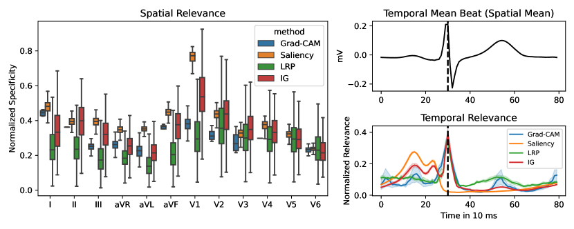
(a) P-wave amplitude (XResNet)

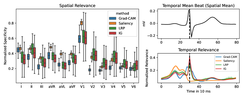
(b) P-wave amplitude (LeNet)

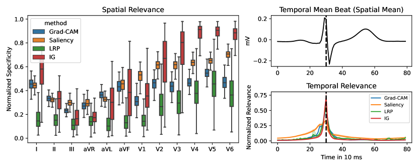
(c) R-peak amplitude (XResNet)

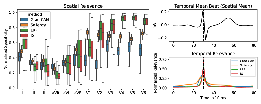
(d) R-peak amplitude (LeNet)

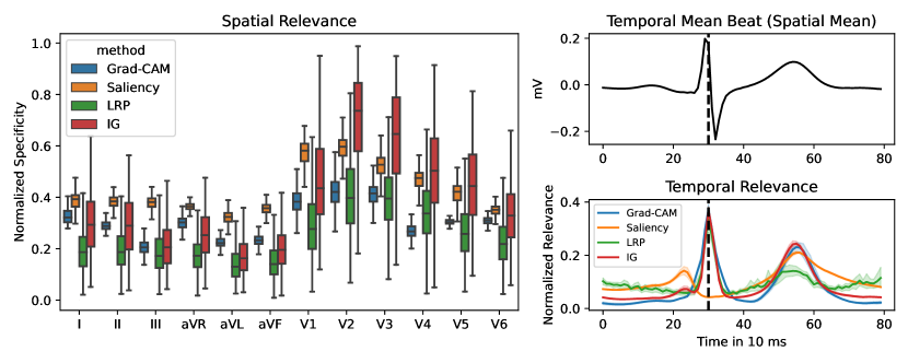
(e) T-wave amplitude (XResNet)

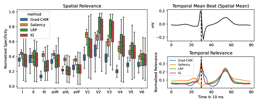
(f) T-wave amplitude (LeNet)

Figure 2: Results of the experiments as described in Section 4.4 of all three considered experiments: P-wave amplitude (Fig. 2(a), Fig. 2(b)), R-peak amplitude (Fig. 2(c), Fig. 2(d) ) and T-wave amplitude (Fig. 2(f)) for LeNet and XResNet, respectively. Each subplot is organized in the same way: On the left, we show spatial specificities with different attribution methods color-coded. In the lower right plot, we show temporal specificities with different attribution methods color-coded. These properties are computed for all samples and their attributions are concatenated to allow for analysis across the whole dataset. For spatial specificity, we consider boxplots, where the leads are on the x-axis and the specificity is on the y-axis. For temporal specificity, we consider continuous line-plots, where time is on the x-axis and the temporal specificity is on the y-axis. In the upper right plot, we provide a median beat as a reference for better localization. we compute the median beat attributions across the whole dataset and scale them to have a norm of one. If only the segment in the lead under consideration was relevant, the spatial specificity would be one, and the temporal specificity strongly peaked around the corresponding segment. In terms of spatial specificity, saliency shows the highest specificity among the limb leads with a comparably small variance. For temporal specificity, all methods attribute more relevance to the QRS complex than to the interval in question, which questions their validity.

We consider four different attribution methods that are widely used either in the ECG domain or in the broader XAI community, in particular in the context of image data: Layer-wise Relevance Propagation (LRP) [40], Integrated Gradients (IG) [41], Gradient-weighted Class Activation Mapping (GradCAM) [23], and Saliency maps [29]. All of them belong to the family of post-hoc attribution methods which attribute relevance to input features as a measure of the feature’s importance for a particular classification decision. Interestingly, applying them to an identical trained model leads to qualitatively different attribution maps, which is a well-known issue in the XAI community [42].

We use ECG parameter regression tasks as sanity checks, i.e., train regression models for both model architectures to predict P-, R- or T-wave amplitudes from the raw signal. The expectation behind this task is that the attributions corresponding to this model should show high temporal and spatial specificity. For example, the prediction of the P-wave amplitude in lead V1 should be strongly influenced by the P-wave in V1, which should be reflected in the corresponding attribution map. We define two measures, the spatial specificity and the temporal specificity, to quantify how effectively the method prioritizes the correct lead or temporal segment in the ECG. The results of the sanity check are compiled in Fig. 2.

Comparing spatial specificities across all experiments, we observe a largely consistent ranking among methods and leads: while LRP and IG are most specific in the precordial leads (V1-V6) followed by saliency, in the limb leads (I, II, III, aVR, aVL, aVF) saliency is the most specific method. Furthermore, we observed significantly less variance in the attributions for saliency, particularly in comparison to LRP and IG. These observations provide a first argument in favor of saliency, as we prefer methods that provide reliable results across all samples rather than only on average. Generally, attributions are significantly more specific in the precordial leads than in the limb leads (especially in V1, V2 and V3). We relate this to the fact that only two of the six limb leads are independent, whereas the remaining four can be computed as linear combinations of any two given limb leads. This leads to strong correlations, in particular among the limb leads, which cannot be disentangled without any further assumptions. The analysis of the cross-correlations among leads in Fig. 11 in the supplementary material, shows significantly less cross-correlation in V1 and V2 as compared to the other leads, which is also reflected in the overall largest absolute spatial specificities in Fig. 2.

In terms of temporal specificity, IG and LRP, which are both constrained by completeness properties (i.e. the sum of attributions equals the output prediction up to approximation effects) attribute the largest fraction of relevance to the R-peak even if the R-peak is not directly relevant for the given task (e.g., for predicting the P-wave or T-wave amplitude). Interestingly, a similar effect is observed for GradCAM. It is not completely implausible that the model could use the R-peak for localization within each beat and therefore could also attribute relevance to the R-peak. If we impose as a necessary condition for sensible attributions that when predicting a particular amplitude, the region around the corresponding segment should show the overall largest attribution across the entire temporal attribution plot, saliency is the single XAI method, which satisfies this condition in all six experiments. This result clearly speaks against all considered methods apart from saliency, which we, therefore, consider as only reference attribution method in the following experiments.

2.2 Global XAI: Does the model exploit cardiologists’ decision rules?

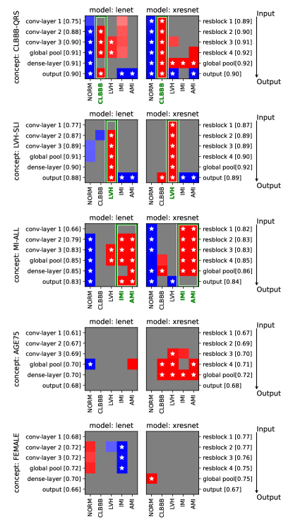
Figure 3: Concept-based analysis: Investigating which of five concepts (from top to bottom: CLBBB-QRS, LVH-SLI, MI-ALL, AGE75, FEMALE) are used consistently for the prediction of a certain class in LeNet(left) vs. XResNet(right). Within a block (i.e., a particular concept-model combination to be tested) rows denote different layers in the model and columns represent the different output classes. TCAV values are colored in red (blue) if larger (smaller) than 0.5, i.e., if they have a positive (negative) influence on the prediction score of a particular class. Stars indicate prediction intervals that do not overlap with 0.5, i.e., correspond to cases where concepts are consistently exploited. The numbers in brackets are the respective CAV accuracies, which describe how well a concept can be linearly separated.

The aggregated attribution maps are an effective tool to highlight which parts of the signal are most relevant for certain decisions/predictions. However, it remains unclear whether, for example, low or high voltage amplitudes or the particular morphology at the location are decisive for the attribution of a signal, let alone how cardiologists’ decision rules can be related to the model behavior. For this reason, we draw on Testing with concept activation vectors (TCAV)[35] as a complementary approach, which, in contrast to the attribution methods discussed so far, allows to test a trained model for its alignment with human-comprehensible concepts. These concepts are defined through examples and can therefore include abstract concepts and relate to specific hidden layers of the model. Accordingly, the TCAV scores, which quantify how a specific concept is exploited, depend on the hidden layer and may vary between different layers. Our aim is to use it to provide insights that generalize across different training runs for a given model architecture. This goes beyond the usual TCAV setting, where only a single model instance is considered. Without loss of generality, we focus on a single well-established concept for each of the three pathologies CLBBB, LVH and MI (in addition to age and sex as two concepts that are not pathology-specific to demonstrate the versatility of the approach).

Fig. 3 depicts the results of the concept-based analysis. The pathology-specific concepts CLBBB-QRS (indicating QRS width greater than 120 ms [43]), LVH-SLI (indicating a Sokolow-Lyon index larger than 35 mm [44]), and MI-ALL (three criteria on pathological Q-waves [45]) are used consistently throughout all layers of both models, exhibiting a strong positive impact on the model prediction of their related pathologies. This is indicated by the red squares marked with asterisks, which almost entirely fill the green rectangles, which highlights the TCAV values of the pathologies matching the corresponding concepts. Interestingly, both CLBBB-QRS and MI-ALL show a consistently negative effect on the prediction of the normal class, which we consider as a consistency check confirming the validity of our analysis. In the case of LVH-SLI, there is no consistent effect on the prediction of the normal class, which aligns with a sizable number of normal samples satisfying the criterion [46].

Summarizing the investigation of the first three pathology-specific concepts, this experiment shows in a so far unseen, consistent fashion that across both model architectures, the concepts are exploited and have a positive effect on the classes they were designed for. The fact that concepts, in a few cases, are also exploited for other classes simply reflects the fact that the rules are not perfectly specific and are additionally influenced by co-occurring diseases. For example, the negative impact of the concept LVH-SLI on MI predictions aligns with decreasing R-amplitudes for MIs, as opposed to increasing R-amplitudes for LVH.

For LeNet, the AGE75 concept (indicating a patient aged 75 years or older) exhibits some negative influence on the prediction of the normal class. In contrast, for XResNet, the concept is exploited differently in terms of a positive effect on the predictions of the four considered pathologies. Finally, the concept FEMALE has a negative effect on IMI for the LeNet and seems to have a positive influence on NORM for one layer of the XResNet, which is most likely related to the different prevalence of pathologies in the PTB-XL dataset comparing men and women.

2.3 Glocal XAI: Insights from aggregated aligned attributions

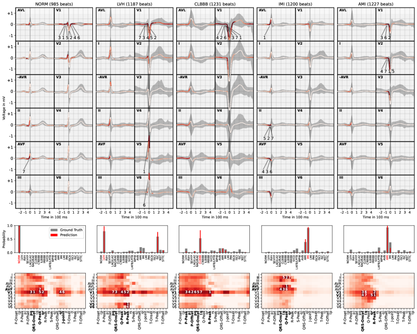
Figure 4: Results of the glocal (dataset-wide) analysis for saliency as an attribution method for a XResNet model. Here, we consider five classes: 1. NORM normal ECG as reference 2. LVH left ventricular hypertrophy 3. CLBBB complete left branch bundle block 4. IMI (chronic) inferior myocardial infarction and 5. AMI (chronic) anterior myocardial infarction. For each class, we aggregate a median beat for the top 100 predictions per class and also provide the mean of ground truth labels (gray bars) as compared to the prediction (red bars) below each plot (see LVH for inter dependencies with _ISC). On top of each plot, we visualize the absolute attributions color-coded, where deep red indicates high attribution for the respective diagnosis (e.g. the QS-complex in V1 and V2 for AMI is highly relevant). At the bottom, we show the relevance distribution broken down according to ECG segments with the top 7 segments with thehighest relevance per segment length marked, which allows for quantitative statements about the relevance distribution. These show good agreement with the relevant segments used in decision rules from clinical literature.

In the XAI literature, one distinguishes local and global attributions, where the former are sample-specific and the latter characterize the entire model. We propose to compute aggregated beat-aligned attributions across entire subgroups with common pathologies to infer global model insights and refer to this approach as glocal XAI.

Fig. 4 summarizes the outcome of this analysis for the five subclasses under consideration in terms of median beats and attributions (top panel), average predictions (middle panel), and in terms of attributions aggregated on segment level for a XResNet model. A largely consistent plot for the LeNet can be found in Fig. 13 in the supplementary material.

2.3.1 Left ventricular hypertrophy (LVH)

The early sign of LVH (left ventricular hypertrophy) is an increase in R-amplitude, which is caused by the increased left ventricular mass. That is why the Sokolow-Lyon index is a frequently used, but relatively unspecific diagnostic tool to assist in the diagnosis of LVH. The Sokolow-Lyon index is calculated as the sum of the R-amplitude in V5 and the S-amplitude in V1. The sum must exceed 3.5 mV to be considered an indicator of LVH.

Both models agree on assigning the highest attributions to the R-peaks in V5, V1, and V6 (in that order). They also attribute relevance to the ST-segment in V1. However, the two models differ in the rest of their attributions: the LeNet places slightly more relevance on the R-peak in V2, while the XResNet additionally focuses on the QR-interval and the beginning of the Q-wave (all in V1).

The strong emphasis on the R-peak in V5 and V6 by both models aligns well with its presence in various LVH concepts and rules, such as the Sokolow-Lyon-Index LVH-SLI. However, except for some attribution in V1, there are no indications of S-peak amplitudes, which are part of some LVH decision rules (e.g., LVH-S12,LVH-LI).

2.3.2 Complete left bundle branch block (CLBBB)

In the case of CLBBB, the consequence of the caused conduction disturbance and at the same time the dominant ECG finding is a widening of the QRS complex to at least 120 ms [43]. Further criteria include, for example, a QS-complex or rS-complex in V1 [47].

First of all, both models focus strongly on V1, with the R-peak in V2 as the only minor exception (for LeNet). Both models put most attribution on the R-peak in V1. Further relevance is attributed to the second half of the P-wave and the PQ-segment, as well as the beginning of the ST-segment. The models differ in their emphasis: XResNet focuses more on the Q-wave, while LeNet places more emphasis on the ST-segment (all in V1).

One might speculate that the attribution maps reveal a focus on the smoother morphology of the onset of the QRS complex compared to normal samples. On the other hand, it is difficult to determine the significance of the QRS width in an attribution map (which was found to be consistently exploited by both models, as shown in the global XAI analysis in Section 2.2). The strong focus on V1 is consistent with decision rules that are based on large QS or rS-complexes in this lead, V1.

2.3.3 Anterior/inferior myocardial infarction (AMI/IMI)

For the characterization of ECG changes related to chronic myocardial infarction, we use the consensus definition [45], which focuses particularly on pathological Q-waves. For the manifestation of the localization of anterior vs. inferior myocardial infarction, we refer to [48] which suggests that AMIs are predominantly detected through QS waves in V1–V3 and IMIs through longer and deeper Q-waves in II, III and aVF.

For IMI and AMI, there is a strong similarity between the aggregated attribution maps of both models. In the case of IMI, both models focus on the Q-peak and the first half of the Q-wave in aVL, II, aVF and III with minor differences in terms of ranking. For AMI, both models focus almost exclusively on leads V1 and V2 and the area between the QRS-onset and R-peak. Both put most relevance on the R-peak and slightly less attribution on the QRS-onset in V1 and V2.

The attributions for both localizations of the chronic MI align very well with the corresponding diagnostic criteria applied in the clinical setting, both in terms of spatial and temporal localization. The clarity and consistency of these patterns across different models is surprising.

2.4 Knowledge discovery: Identifying subclasses using glocal XAI

In this section, we demonstrate the effectiveness of attributions in revealing sub-structures within a model, beyond the granularity of label information. To do this, we first present evidence in a controlled environment using the hierarchical labels provided by PTB-XL. Then, we use this framework to uncover intriguing insights into a shift in the interpretation of female ECGs and the possibility of ASMIs.

2.4.1 Confirmative analysis: Discovery of sub-diagnostic classes of myocardial infarction

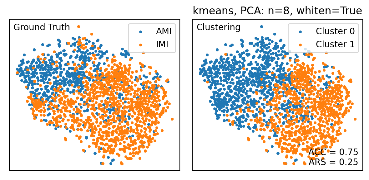
(a) Input

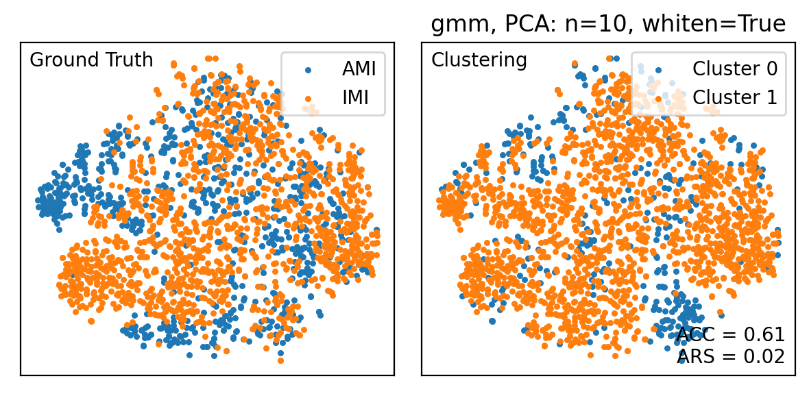
(b) Hidden Features

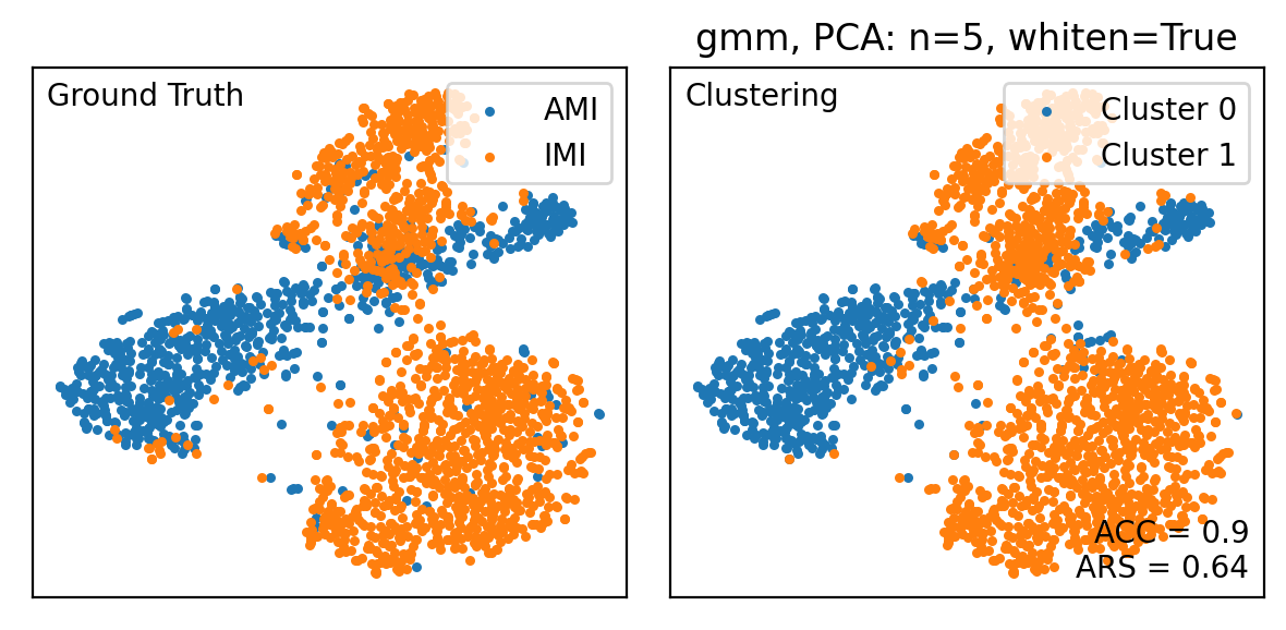
(c) Attribution

Figure 5: Results of the experiments as described in Section 2.4.1. TSNE embeddings (with default parameters each) of three different representations extracted from a XResNet model: Fig. 5(a) for the input median beats, Fig. 5(b) for the hidden features after global pooling and Fig. 5(c) for the saliency attributions. In each subplot, we color-coded the ground truth labels left and the resulting clustering on the right. The plots reveal that (aligned) attributions are the most effective input representation for subclass discovery.

In this section, we propose an experiment to discover sub-diagnostic classes within a super-diagnostic class using aggregated attribution maps as a source for knowledge discovery, instead of input or hidden feature representations. Building on the insights from the previous section (Glocal XAI), we focus on the differentiation of myocardial infarctions (MI) into anterior (AMI) and inferior (IMI) myocardial infarctions (see Section 2.3.3). For this, we train a model capable of classifying into five super-diagnostic classes (including MI). Once trained, we fit clustering models on all samples labelled as MI (specifically we filter for samples that were labeled with MI as the exclusive super-diagnostic label and either uniquely AMI ($n=702$) or IMI ($n=1250$). In order to provide evidence for the efficiency of (1) attribution maps in discovering sub-diagnostics, we consider the following representations as baselines: (2) median input beats and (3) features from deeper layers of the trained model.

In Fig. 5, we show the results of this experiment, where we observed the best clustering performance on attributions, i.e. an accuracy of 90% for attributions (Fig. 5(c)) compared to 75% for input (Fig. 5(a)) and only 61% for hidden features (Fig. 5(b))

In Fig. 6, both clusters are visualized, with cluster 0 predominantly corresponding to AMI and cluster 1 predominantly to IMI. The median beats for both clusters were computed by aggregating the corresponding beats, based on the attribution clusters, along with the corresponding mean attributions on top. The resulting clusters agree with the glocal analysis of supervised models in Fig. 4.

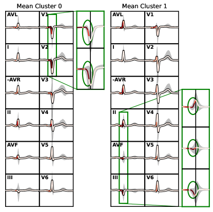
Figure 6: Analysis of the cluster means of the Gaussian Mixture Model fitted on attributions as described in Section 2.4.

2.4.2 Explorative analysis: Identifying subgroups within anteroseptal myocardial infarction

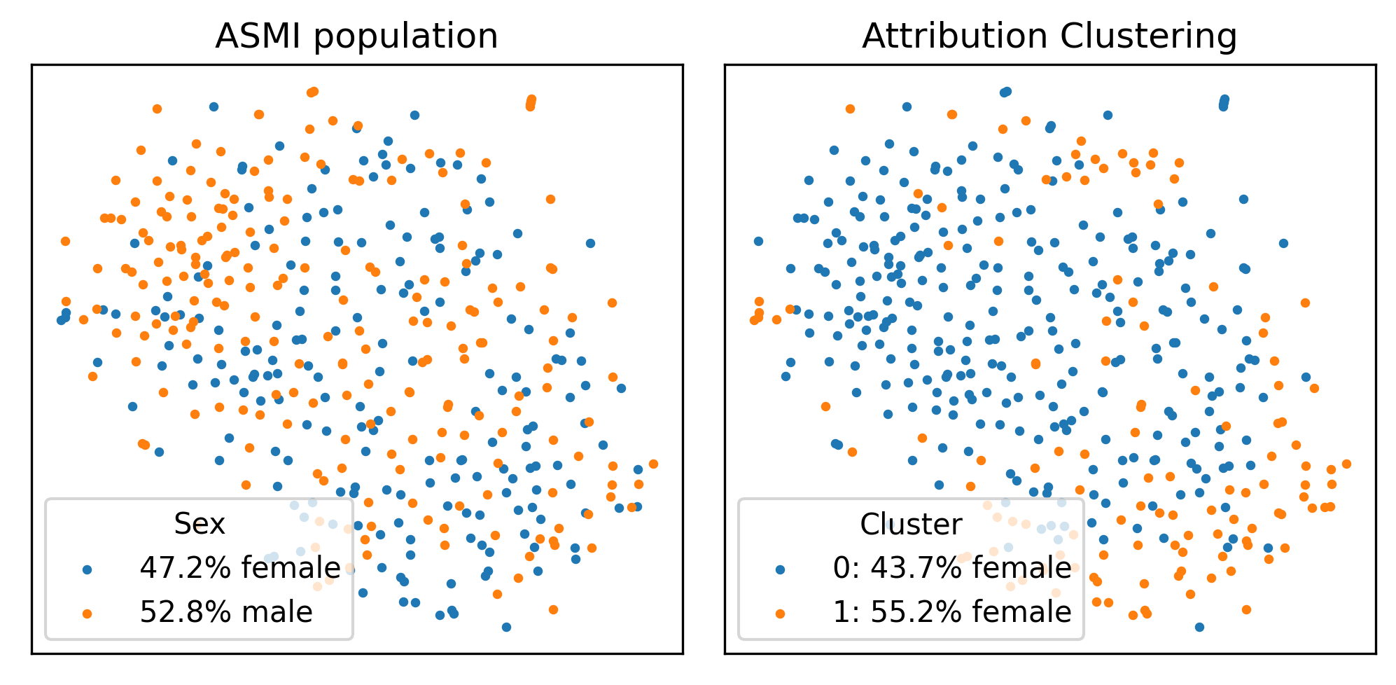
(a) TSNE embeddings for the XResNet model.

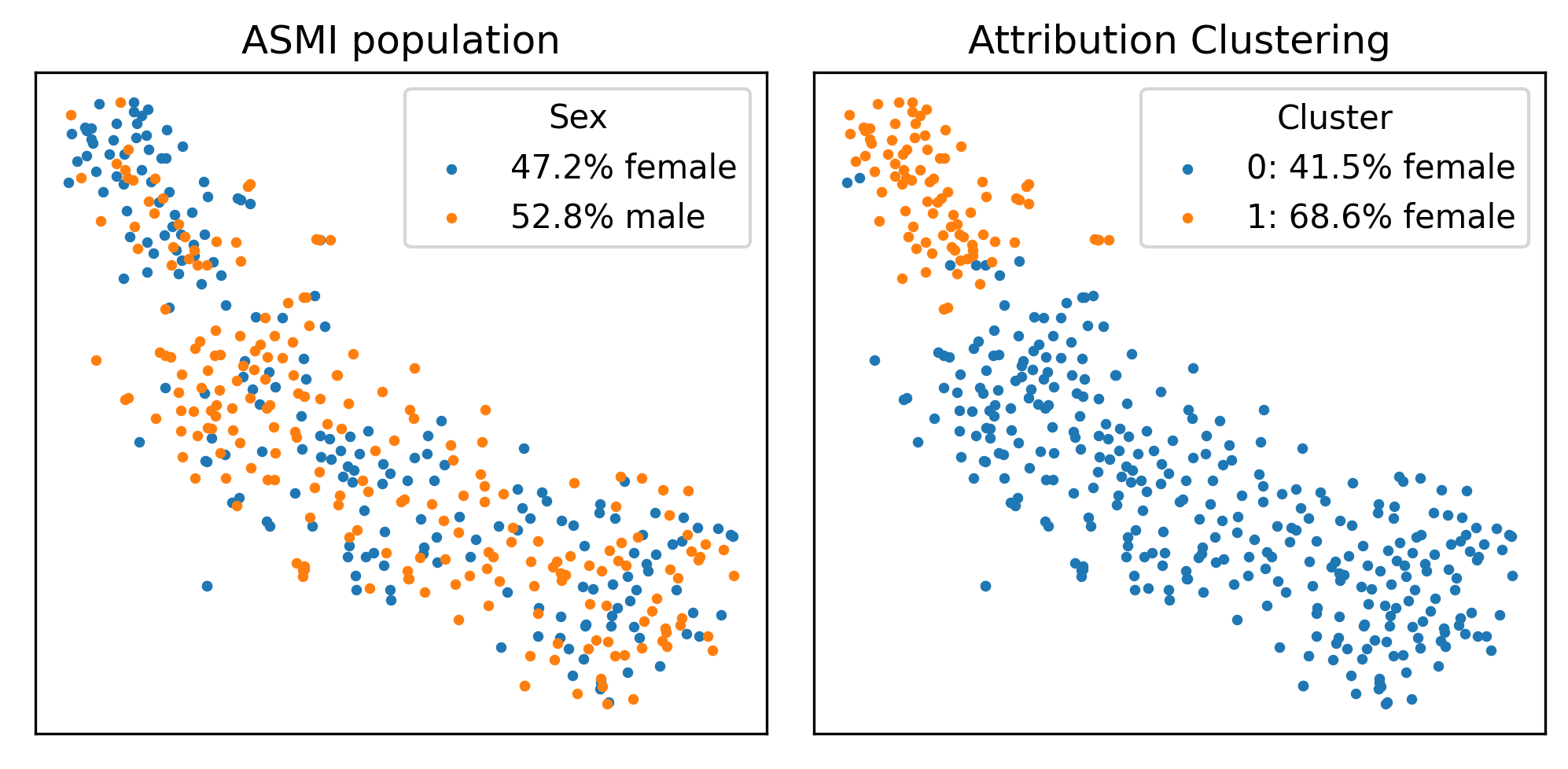
(b) TSNE embeddings for the LeNet model.

(c) Cluster means based on XResNet.

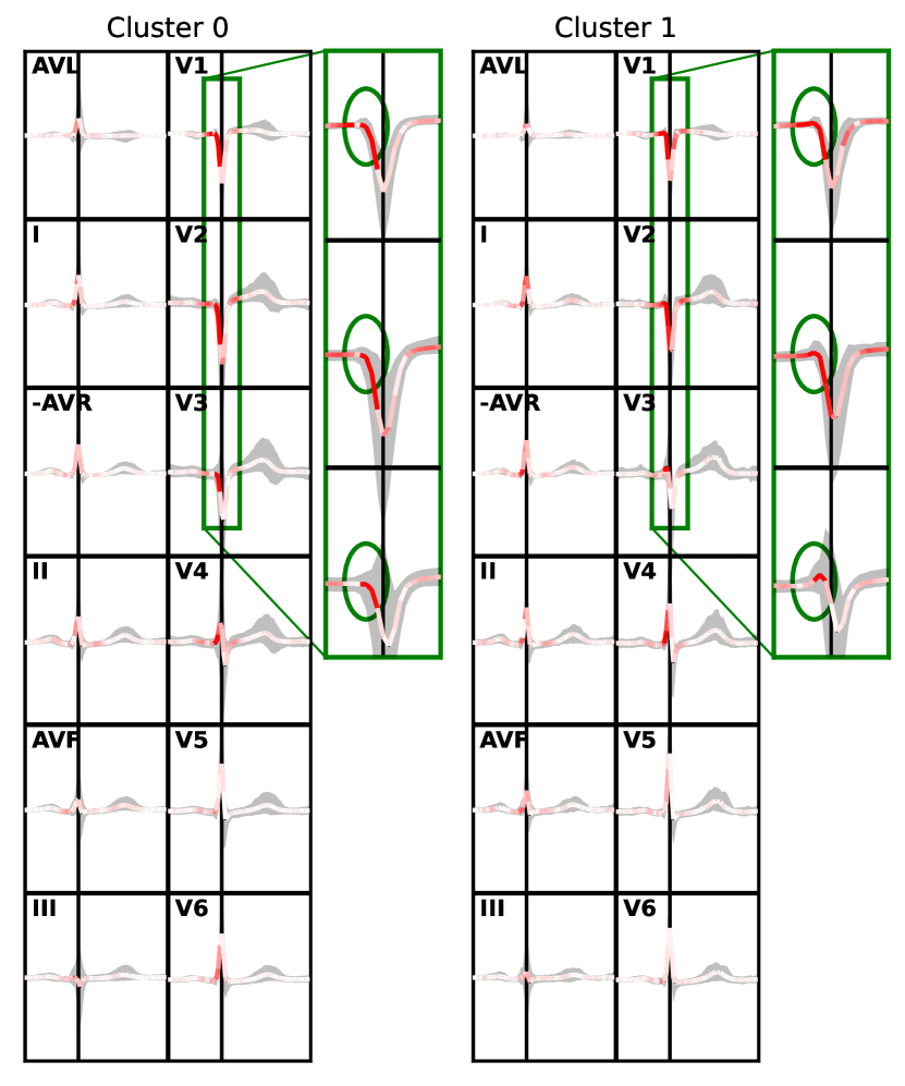
(d) Cluster means based on LeNet.

Figure 7: Explorative analysis of the substructure of the ASMI (anteroseptal myocardial infarction) for the XResNet model on the left (Fig. 7(a) and Fig. 7(c)) and LeNet model on the right (Fig. 7(b) and Fig. 7(d)). Top plots Fig. 7(a) and Fig. 7(b): TSNE embeddings (based on attributions) for ASMI colored by sex (left) and cluster assignment (right, as in Fig. 5(c)) reveals two distinct clusters. Bottom plots Fig. 7(c) and Fig. 7(d): Corresponding cluster means and median beats for ASMI attribution clusters reveal distinct morphological differences, which can be associated with different degrees of severity of the myocardial infarction. Encircled regions in the plots indicate regions where the difference between the corresponding attributions, which are used for clustering, are significantly different from zero, i.e. the main regions where one expects to find differences between both clusters. These reveal a cluster of transmural ASMIs (cluster 1) and a cluster of less severe ASMIs and according to modern diagnostic standards even normal variants (cluster 0).

We go one step beyond confirmation and demonstrate how the proposed approach can be used to identify clinically relevant structures for pathologies, where no further substructure is known. Here, we focus on a particular sub-condition, the anteroseptal myocardial infarction (ASMI), which is one of the two most frequent myocardial infarction localizations in PTB-XL.

Using the method from the previous section, we cluster the aligned attribution maps for all ASMI samples and visualize the corresponding embeddings in Fig. 7(a) and Fig. 7(b) for XResNet and LeNet, respectively. In Fig. 7(c) and Fig. 7(d) we visualize the mean beats corresponding to the respective clusters, where we highlight the regions of interest via ellipses. Interestingly, both model types identify similar clusters highlighting the area before the vertical line in leads V1, V2, V3.

The main difference between the clusters is the presence or absence of an R-peak. In the case of the LeNet, see Fig. 7(d), a remnant R-peak is clearly visible in cluster 1 in all three leads V1, V2, V3, in the case of the XResNet only in V3 and V2. In both cases, cluster 0 shows clear signs of a transmural anteroseptal myocardial infarction, in particular, no visible R-peaks in leads V1, V2, V3. As the size of the R-peak is indicative for extension of the scar, cluster 0 hence encompasses ASMIs of a less severe degree.

Going beyond a descriptive analysis, we aim to explore the potential clinical meaning of these results and identify sex as the most significant covariate discriminating both clusters. And indeed, for women such ECG changes are in some cases even considered as normal variants [48], which aligns very well with the majority of female samples in this cluster 1 (XResNet: 55% LeNet:69% all ASMIs: 53%). This is also supported by the mean predicted probabilities for the non-transmural cluster 1, both models show a reduced AMI probability (compared to the set of all ASMI predictions) and an increased NORM probability. Again, this pattern is most clearly exposed in the case of the LeNet (AMI 0.27 and NORM 0.41 on cluster 1 as compared to AMI 0.72 and NORM 0.09 on all ASMI samples). Indeed, the explicit inspection of a subset of 10 female samples of the LeNet cluster 1 revealed that these would be diagnosed as normal variants according to modern standards, whereas they would have been diagnosed as ASMIs due to R-progression according to the common diagnostic standards at the time the PTB-XL dataset was created.

3 Discussion

We propose sanity checks based on an ECG parameter regression task. Surprisingly, three out of the four considered attribution methods do not show a sensible degree of temporal or spatial specificity and show a strong bias toward attributing relevance to the QRS-complex, which typically contains the highest signal amplitudes. In particular, GradCAM, the most widely used attribution method in the field of ECG analysis, fails to satisfy the sanity check. Saliency maps, the only method that passed the sanity check, show a high degree of temporal specificity. Gradient noise, a major drawback of saliency methods, can be very effectively reduced by aggregating attributions across beats and samples. The outcome of the sanity check not only call into question results achieved using attribution methods that did not pass the sanity check in the field of ECG analysis, and serves as a warning against blindly applying of off-the-shelf attribution methods in any domain.

We see the ability to test if deep learning models exploit a certain (abstract) concept as a decisive advance in the global analysis of ML models. It provides crucial new insights into the model that are difficult to attain with conventional attribution methods. The ECG domain is particularly well-suited for this purpose due to the availability of large rulebooks comprising decades of cardiologists’ expert knowledge, which are mostly formulated in terms of ECG features that can be automatically extracted from the signal. We demonstrated the potential of this technology for selected concepts and pathologies and found a compelling alignment with expert knowledge. We envision that this approach could serve as a component to assess the internal validity of a machine learning algorithm during the certification process for automatic ECG analysis algorithms. On the one hand, it allows for the verification of certain concepts that are considered to be mandatory for every model deployed in clinical environments. On the other hand, it can also be used to check whether concepts related to sensitive attributes are systematically exploited. This provides a complementary perspective to the fairness literature, which mostly relies only on model performance, see e.g., [49], and addresses on the fundamental question of whether the model should be allowed to exploit sensitive attributes for its decision.

Most of the existing applications of attribution methods in the field demonstrate insights based on single hand-picked examples. Our analysis provides strong arguments in favor of aligned attribution maps, which can be defined on beat level or even on the level of individual ECG segments composing the beat, that can be aggregated across entire patient subgroups. To summarize, our analysis shows an unexpectedly strong similarity between the attribution maps of both model architectures, in particular also in terms of ranking of the most relevant segments. The quantified attribution distribution onto segments and leads can be used to compare to cardiologists’ decision rules. We find good agreement for the most relevant parts both in terms of spatial and temporal localization. This technique finds its boundaries when decision rules can no longer be directly related to single ECG features but to more abstract concepts, which could be analysed in the global XAI section. To the best of our knowledge, we are the first to make such statements in a quantitative manner broken down according to leads and segments in a dataset-wide analysis as opposed to anecdotal evidence based on single hand-picked examples. This technology could serve as a complementary assessment of the internal validity during a certification process but can also be used for knowledge discovery.

We demonstrate that aligned attribution maps represent the most reliable way of identifying subclasses within a given superclass (compared to aligned raw signals or hidden features), which is a surprising observation. It crucially relies on the alignment, which is non-trivial to be achieved in other data domains. However, similar techniques have been used in the literature to identify spatially localized artifacts compromising image classifiers [50]. Concept-based methods that directly relate to structures in the models’ hidden representations [51] might be a way to overcome the limitations of the requirement of aligned samples and might provide a characterization on the level of individual segments rather than entire beats.

Applying the same approach to anteroseptal myocardial infarctions, we demonstrate that the method can distinguish transmural from non-transmural myocardial infarctions as clinically meaningful subgroups. This goes as far as providing hints on the internal consistency of diagnostic classes. We see the ability to question diagnostic knowledge through data-driven insights as a promising path to advance the field of ECG analysis providing insights that even extend to diagnostic criteria underlying the different conditions. Here, the most accurate model does not necessarily allow the deepest insights. The more complex XResNet has sufficient model capacity to learn essentially arbitrary input-output patterns. However, the shallower LeNet, due to its smaller model capacity, reveals the tension between the NORM condition and the diagnostic criterion used to diagnose ASMI. Extending this approach to further pathologies to deepen the understanding of ECG signs through such a combination of data- and model-driven techniques represents a promising perspective for future research.

4 Methods

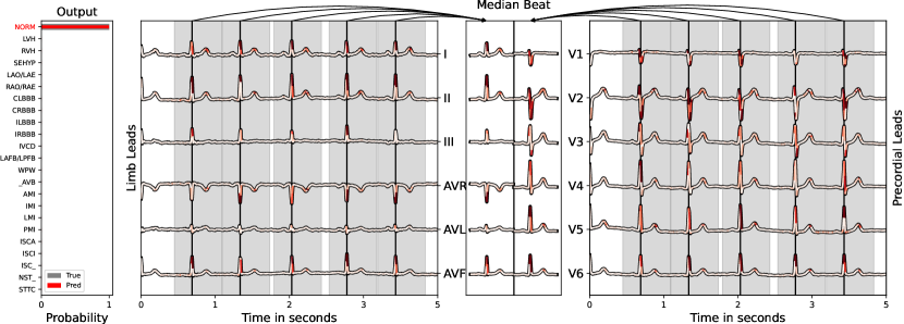
Figure 8: Example 12-lead ECG with saliency attributions color-coded on top of the signal, where deep red indicates high attribution for the given model’s output. In order to allow for aggregation of the median beat (centered in the plot), we provide R-peaks as vertical lines along the signals which are used to crop 300 ms before and 500 ms after each peak (gray boxes around R-peaks).

This section is organized as follows: In Section 4.2, we introduce the dataset and the models used for our analysis. In Section 4.3, we introduce local XAI methods, along with task-specific sanity checks and beat-level aggregation. Finally, in Section 4.5, we provide a complementary perspective from the point of view of concept-based XAI. Fig. 1 provides a schematic overview of the different components of the proposed approach and their interrelations.

4.1 Pathologies

The left bundle branch block is a blockage or severe delay in electrical conduction in the left tawara (bundle branch) branch or fascicles. The septum is not excited from left to right, but from right to left. The main QRS vector therefore initially points to the left and forward. The delayed excitation of the muscle-strong left ventricle is reflected in the broad QRS complexes. A review on LBBB criteria [47]includes, in addition to the widening of the QRS complex, a QS complex or rS complex in V1.

Myocardial infarctions are called anterior/inferior myocardial infarctions depending on whether they involve the anterior wall or inferior wall. Chronic myocardial infarctions are mainly identifiable via pathological Q-waves [48]. The relevance of the channels depends on the localisation of the myocardial infarct. For AMI, it describes vanishing R-waves and appearing QS-waves in anterior leads V1 and V2 and with increased extension also V3. For IMI, longer Q-waves are found in the inferior leads II, III and aVF. We stress at this point that what we are referring to as myocardial infarctions (MIs) are chronic as opposed to acute MIs, which account for the vast majority of MIs in PTB-XL. This is an important distinction as the diagnostic criteria differ for chronic as compared to acute MI.

Left ventricle hypertrophy describes an increase in the mass of the left ventricle. The increased mass causes an increase in the R-Amplitude. Further, the effect is compounded by a shift of the QRS axis to the left and a convergence of the hypertrophied heart towards the chest wall. In connection with a reduced coronary perfusion reserve and subendocardial ischemia, T-wave changes result (initially T-flattening, later a T-negativation). It is important to stress that LVH shows a complex continuum of different stages [48], which cannot be resolved here due to a binary annotation in the PTB-XL dataset.

4.2 Data & Models

We base our experiments on the PTB-XL data set [37, 38, 39], which covers 21799 ECGs from 18869 patients annotated with ECG statements from a broad set of 71 statements covering diagnostic statements and form- and rhythm-related statements. We focus on the 23 statements at the sub-diagnostic level to allow a sufficiently finegrained analysis without adding the complexity of the full set of 44 diagnostic labels, some of which are only sparsely populated. We follow the benchmarking protocol for PTB-XL, which was put forward in [5], which uses eight of the ten stratified folds for training and the remaining two for validation (model selection) and testing. As in prior work, we use the macro average of the area under the receiver operating curve as performance metric. The ECG features that are used for the concept-based explainability methods, see below, are extracted by the University of Glasgow ECG analysis program [52].

In terms of model architectures, we work with convolutional neural networks as they are to date the predominantly used model architecture in the field, see e.g.,[7, 53, 10], even though recent works suggest that recurrent architectures [54] or structured state space models [55] might further improve over the convolutional state-of-the-art. We consider both a shallow model inspired by the LeNet architecture [56] and a ResNet-based [57] architecture, which was shown to lead to competitive results [5] for ECG classification tasks on PTB-XL. The two model architectures are described in more detail below:

LeNet: shallow model inspired by the LeNet architecture [56], which is composed of 3 one-dimensional Convolutional Layers (with kernel size 5, stride 2 and output channels 32, 64 and 128, respectively), interleaved with BatchNorm, ReLU and pooling layers (the first two pooling layers are MaxPool and the last one AvgPool). This is followed by two fully-connected layers, again interleaved with ReLU as activation.

XResNet: ResNet-based [57] architecture, which were shown to lead to competitive results [5] for ECG classification tasks on PTB-XL. More specifically, we use a one-dimensional adaptation of the XResNet architecture[58], which is described in detail in [5]. In our experiments, we use a xresnet1d50 architecture.

The task is framed as a multi-label classification task and consequently, binary cross-entropy is used as optimization objective. We work at a sampling frequency of 100 Hz and use input sizes of 250 tokens, corresponding to 2.5s, which were shown to lead to the best results for the given task [55].

4.3 Local XAI

The XAI community has put forward a range of post-hoc interpretability methods, which can be used to assess the attribution of input features. These methods commonly provide an attribution (map), which shares the shape of the input and indicates the relevance of particular parts of the input sequence for a classification decision at hand. This allows us to temporally resolve the most relevant parts of the sequence but also to identify the most discriminative leads for a particular condition. We consider and compare four different XAI methods that are either predominantly used in the ECG community or are popular choices in the XAI community. More specifically, we consider GradCAM [23], saliency maps [29], integrated gradients (IG) [41] and layer-wise relevance propagation (LRP) [40], where the latter is equivalent to gradient * input in the case of ReLU activations [59]. Saliency maps explain model predictions by using the norm of their respective input gradients. GradCAM attribution maps consist of a (feature depended) weighting of the activation gradient of the respective model prediction. Integrated Gradients (IG) creates attribution maps by integrating the input gradient (of a chosen output neuron) from a predefined baseline input to the sample under consideration. Layer-wise Relevance Propagation (LRP) propagates the model prediction from the output neuron back to the input. In each layer, an attribution is assigned to each neuron using the LRP rules, which (approximately) preserve the sum of attributions across layers.

4.4 Sanity checks

The first sanity check relies on ECG parameter regression. The intuition behind this experiment is the expectation that a model that was trained to regress a particular amplitude in a particular lead from the raw signal should focus spatially on this particular lead and temporally on the corresponding segment. To implement this experiment, we fit a regression model to a feature present in each lead (P-wave, R-wave and T-wave amplitude), i.e. a model with 12 output neurons, one for each lead feature. For this, we used the same model architectures introduced above and use the mean squared error as optimization objective. As regression targets we use ECG parameters extracted by the University of Glasgow ECG analysis program [52], a commercial ECG analysis software. For a given sample and a chosen lead $L$ which we use for parameter regression, we compute an attribution map $(\mathbf{a}^{L})_{tl}$ (where $t=1\ldots T$ and $l=1\ldots 12$). In order to compare across different methods, the attribution maps are analyzed both spatially as well as temporally.

We define a measure $(s^{L})_{l}$ for the spatial specificity as follows:

First, we compute temporally aggregated attributions $(\mathbf{\tilde{a}}^{L})_{l}$ by computing euclidean norm of the attribution map $(\mathbf{a}^{L})_{tl}$ along the temporal direction ($t$). We define the spatial specificity $s^{L}_{l}$ as the ratio between temporally aggregated attribution in the target lead, $(\mathbf{\tilde{a}}^{L})_{L}$ and the euclidean norm of the temporally aggregated attributions $(\mathbf{\tilde{a}}^{L})_{l}$ along the remaining channel dimension ($l$). We visualize the median and quantiles over all samples and obtain in this way a spatial specificity score for each lead $L$, which can be visualized in terms of boxplots.

This ratio is close to one if the attribution is specific to the lead in question. We expect a sensible attribution method to be spatially specific. We also define a measure $(t^{L})_{\tau}$ for the temporal specificity as described below:

We extract temporally aligned (beat-wise) attributions by cropping from 300ms before until 500ms after the R-peak $(\mathbf{b}^{L})_{b\tau l}$, where $b=1,\ldots,B$ enumerates the number of beats in the sample and $\tau=1\ldots 80$. We compute spatially aggregated attributions $(\mathbf{\tilde{b}}^{L})_{b\tau}$ by calculating the euclidean norm along the channel axis ($l$) of $\mathbf{b}^{L}_{b\tau l}$. Then we define the temporal specificity $(t^{L})_{\tau}$ as the median of $(\mathbf{\tilde{b}}^{L})_{b\tau}$ over all beats ($b$) from all samples entering the analysis. We additionally take the median across all leads $L$ as we are not interested in resolving the temporal specificity of single channels.

4.5 Global XAI

We base our approach on TCAV [35], which allows testing a trained model for alignment with human-comprehensible concepts. Concepts are defined through examples and can therefore include also abstract concepts. First, a vector (CAV) encoding the meaning of the concept is trained using the collected examples. Second, the gradient of pathology predictions in the direction of the concept vector is calculated to assess whether the trained model uses the concept for the prediction of those pathologies. The definition of a concept is in this case always tied to a chosen hidden feature layer in the model architecture, where one expects that low-level concepts that directly relate to signal features are most clearly expressed in feature layers close to the input layers, whereas more abstract concepts at a higher semantic level are expected to be found in higher feature layers. Therefore we always include a range of different feature layers in our analysis.

First, we create a binary data set per concept, each consisting of positive examples of the concept and randomly drawn data points that do not contain the concept. Second, we use these datasets to train a linear classifier in the feature space of a hidden layer for each concept. We interpret the accuracy of the linear classifier as a measure of how well the concept can be defined in said feature space. The classifier then yields the concept activation vector (CAV), which we use to compute the TCAV values via directional derivatives, see the technical description in App. A.5).

This definition relies on the linear separability of positive and negative samples in feature space, which we assess via the accuracy of the linear classifier on which the CAV is based (prerequisite 1). To circumvent accidental findings, the process is carried out for 10 CAVs for 10 trained models with different seeds. It is worth mentioning, that the negative samples are resampled at each CAV fitting. From these 100 TCAV values, we extract 0.05 and 0.95 percentiles. We are interested in observing consistent model behaviour and therefore exclude all concepts where the above confidence interval spans more than 0.5 (prerequisite 2). If the confidence intervals do not overlap with 0.5 (indicating that the concept is neither consistently exploited in a positive nor in a negative fashion), the concept does not have a consistent impact on the model (prerequisite 3). If the prediction interval lies above(below) 0.5 it has a consistent positive(negative) impact on the model prediction of the particular class under consideration. We base our discussion on which concepts are consistently used in particular models on those concepts that fulfill all three prerequisites.

4.6 Glocal XAI

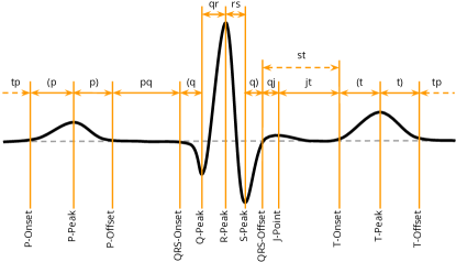
Figure 9: Our used segmentation/annotation schema based on ECGDeli [60] fiducial points (lower annotations), enriched by segments (upper annotations).

We aim to align attribution maps based on beats, i.e. R-peaks, or alternatively based on ECG segments. Both require an ECG delineation as a first step. For this, we trained a model capable of segmenting 12-lead ECG samples into 24 different segments. For our purpose, we trained a 2d U-Net [61] with convolutional kernels that span the entire feature axis. The crucial advantage of this approach compared to conventional ECG delineation models is the ability to exploit the consistency of segmentations across several leads as opposed to segmenting all leads individually. As labels we used fiducial points extracted from ECGDeli [60] for PTB-XL (as segments of length 1) as well as the segments between them, see Fig. 9, leading to a total of 24 different segments. In general, given a 12 lead ECG sample of length L $\mathbf{x}\in\mathbb{R}^{L\times 12}$, our segmentation model $S:\mathbb{R}^{L\times 12}\rightarrow\mathbb{R}^{L\times 12\times M}$ computes for each timestamp a soft assignment score for all $M$ segment classes (which can be interpreted as a probability distribution over all M segment classes). The model is trained with random patches minimizing the categorical cross-entropy with the Adam optimizer. The model showed strong results and showed good overlap with the ground-truth annotations, but also showed more reliable segmentations based on a manual inspection in cases of disagreement with ECGDeli. We defer a detailed performance analysis of this model to future work.The ECG-features for the concept-based analysis were taken from the PTB-XL+ dataset [62]. We provide soft segmentation maps [63] for the entire PTB-XL dataset.

We perform a robust R-peak detection based on the soft predictions for the R-peak class in the segmentation. We perform a peak detection (distance of 30 timestamps and minimum output probability of 0.25) based on the spatial maximum of V1-V4. The R-peaks identified in this way are part of the data repository released with this paper. We then extract median beats from the signal by extracting the signal 300 ms before until 500 ms after each identified R-peaks. We proceed similarly for the attribution maps to extract corresponding beat-centered attribution maps. We can then aggregate the signal to derive representative median beats across several beats within a given sample but also across entire subsets of patients, which share a common pathology. To illustrate the aggregation procedure, we provide an example of (a 5s segment of) one 12-lead ECG signal together with attributions. In this particular case, we want to demonstrate the following basic principles: 1. 12-lead ECG of arbitrary length (minimum of 2.5 seconds) is diagnosed as NORM with high confidence. 2. on top of the signal we visualize the attribution for this diagnosis. 3. Moreover we highlight the respective R-peaks which are used to crop and compute the median beat of this signal. The center of the plot shows the corresponding median beat superimposed with the corresponding attributions.

For Fig. 4 and Fig. 13, we perform experiments on entire subgroups of pathological samples by filtering the top 100 model predictions per class as these most clearly express the patterns exploited by the model.

For the segment-specific parts of Fig. 4 and Fig. 13, the idea is to distribute attributions using the soft segmentation outputs as weighting factors. To this end, we computed the aggregated maps $\mathbf{m}\in\mathbb{R}^{12\times M}$ of the raw signal $\mathbf{x}\in\mathbb{R}^{L\times 12}$ and the segmentations $\mathbf{s}\in\mathbb{R}^{L\times 12\times M}$ (similar for the attributions) as $\mathbf{m}_{i}=\mathbf{x}_{:,i}^{\top}\mathbf{s}_{:,i,:}$ for each i in 1,…,12 where each $\mathbf{m}_{i}\in\mathbb{R}^{M}$ is concatenated to $\mathbf{m}=\left[\mathbf{m}_{1},\ldots,\mathbf{m}_{12}\right]$ and normalized by temporal sum $\mathbf{\tilde{s}}=\sum_{i=0}^{L}{\mathbf{s}_{i,:,:}}$.

4.7 Knowledge discovery

We complement aligned median beats and attributions by hidden feature representations. Here, we use features from layers after the global pooling operation (present in all our considered models) to ensure translation invariance.

As performance metrics we report (1) standard accuracy (ACC) after assigning the clusters to classes and (2) adjusted Rand score (ARS) suited for comparing similarities among clustering.

In order to avoid issues with dimensionality for clustering, all representations were dimensionally reduced via projecting onto the first $k$ principal components that manage to capture 75% of the total variance. Since each representation differs in multiple unknown properties, there is no single clustering model, which is best-suited for all representations. Instead, we carefully selected models and hyper-parameters for each representation maximizing the clustering scores. In this sense, our result is a confirmative study indicating the best possible score (within the range of considered clustering algorithms and hyperparameters) that can be achieved given the ground truth label assignments. The best clustering results were achieved for (1) attributions and (3) hidden features using Gaussian Mixture Models (GMMs), for (2) inputs using k-means.

We demonstrate a structured procedure to gain further insights into the identified clusters. To this end, we plot the (aligned) mean attributions of both clusters and identify temporally as well as spatially localized regions where both deviate most strongly, see Fig. 10. In a second step, we visualize these regions but this time superimposed on the cluster means in terms of the original signals, see Fig. 6 for MI or Fig. 7(c)/Fig. 7(d) for ASMI.

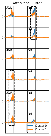
Figure 10: Means of GMM cluster in terms of attributions (MI subclusters as extracted from a XResNet). Localized regions of large deviations pointing towards the most crucial differences between the clusters are marked by dashed rectangles.

Data availability

The PTB-XL dataset underlying this work is publicly available [37, 38]. We provide soft segmentation maps [63] for the entire PTB-XL dataset as computed by our custom segmentation algorithm.

Code availability

We provide the source code to reproduce the main results of our investigations as part of the supplementary material. It will eventually be provided in a publicly accessible code repository after acceptance. The code builds on the XAI software packages captum [64] and zennit [65].

Author Contributions

P.W., T.M., N.S. contributed to the design of the work. P.W. and T.M. contributed the analysis and the creation of models, experiments and results. N.S. supervised the work. All authors interpreted the results, P.W., T.M. and N.S. wrote the first draft and all authors revised it. All authors approved the submitted version.

Competing Interests

The authors declare no competing interests.

Appendix A Supplementary Material

A.1 Data and Models

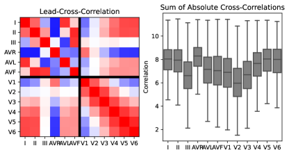
Figure 11: Cross-Correlations among leads showing leads V2, V3 and III have less cross-correlation compared to other leads.

In Fig. 11 we provide cross-correlations among leads highlighting how much the leads in 12 lead ECG signals correlate with each other. This cross-correlation is most prominent in the limb leads, where four out of six leads are synthetic, i.e. a linear combination of the remaining two leads, which are linearly independent. This fact provides evidence for the drop in the performance of attributions methods in terms of spatial specificity in some leads.

For the task of predicting the sub-diagnostic labels of PTB-XL, in terms of macro AUC, i.e. the mean across all individual label AUCs, we observe that shallow convolutional models like LeNet (macro AUC $0.9245\pm 0.0030$) are almost competitive with deep models like XResNet (macro AUC $0.9292\pm 0.0043$). To put this into perspective, we also report the performance on the more comprehensive set of all 71 labels at the most finegrained level in PTB-XL, where we notice a bigger gap between the XResNet model (macro AUC $0.9286\pm 0.0028$) and the LeNet (macro AUC $0.9022\pm 0.0043$). Both values should be set into perspective with the performance of the best-performing models in [5] (sub-diagnostic: macro AUC $0.93$ and all: macro AUC $0.925$).

A.2 Sanity checks

In Tab. 1, we describe the result of the regression experiment introduced in Section 4.4. The results in terms of mean absolute error and coefficient of determination are provided in Tab. 1, showing slight advantages of the LeNet models in two of the three experiments. Overall, each considered model performs reasonably well such that the analysis is not affected significantly by the choice of the model architecture.

Model	MAE$\downarrow$	$\text{r}^{2}\uparrow$
Task	P-Wave Amp.
LeNet	$0.0199\pm 0.0004$	$0.7693\pm 0.0247$
XResNet	$\mathbf{0.0187\pm 0.0004}$	$\mathbf{0.7822\pm 0.0219}$
Task	R-Peak Amp.
LeNet	$\mathbf{0.0602\pm 0.0010}$	$\mathbf{0.9742\pm 0.0021}$
XResNet	$0.0801\pm 0.0013$	$0.9491\pm 0.0026$
Task	T-Wave Amp.
LeNet	$\mathbf{0.0352\pm 0.0008}$	$\mathbf{0.9402\pm 0.0079}$
XResNet	$0.0385\pm 0.0005$	$0.9308\pm 0.0070$

Table 1: Results of regression experiments as described in Section 4.4, where we report mean and standard deviation (obtained by bootstrapping) mean absolute error (MAE) and coefficient of determination ($r^{2}$) for each pair of models (LeNet and XResNet) and task (P- and T-wave and R-peak amplitudes in all 12 leads).

A.3 Global XAI

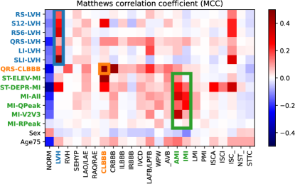
Figure 12: Matthews correlation coefficient (MCC) for all pairs of concepts and pathology.

We summarize commonly used concepts/decision rules for the pathologies considered in this work Tab. 2 along with formalized versions of them in terms of automatically extracted ECG parameters. In Fig. 12, we analyze the overlap between annotations for particular pathologies and specific concepts in terms of Matthews correlation coefficients (MCCs). For the selection of the most discriminative concept for each pathology, we use the concept with the highest MCC value for the given pathology. Therefore, we picked LVH-SLI for LVH, CLBBB-QRS for CLBBB and MI-ALL for IMI/AMI.

	name	description	formalized condition
AMI/IMI	MI-V2V3	Any Q Wave in leads $V_{2}$-$V_{3}$ $\geq 0.02s$	((Q_Dur_V2 $>$0.02) & (Q_Dur_V3 $>$0.02))
		or QS complex in leads $V_{2}$-$V_{3}$ [45]	| ((R_Amp_V2 $=$ 0) & (R_Amp_V3 $=$0))
	MI-RPEAK	R wave $\geq 0.04s$ in $V_{1}$-$V_{2}$ and $R/S\geq 1$ with a	(R_Dur_V1 $>$ 0.04) & (R_Dur_V2 > 0.04)
		concordant positive T wave in absence of conduction defect[45]	& (R_Amp_V1 $>$ 0) & (R_Amp_V2 > 0)
			& (T_Amp_V1 $>$ 0) & (T_Amp_V2 > 0)
			& (abs(R_Amp_V1) $>$ abs(S_Amp_V1))
			& (abs(R_Amp_V2) $>$ abs(S_Amp_V2))
	MI-QPEAK	Q wave $\geq 0.03s$ and $\geq 1$mm or QS complex	(Q_Dur_X$\geq 0.03$) & (abs(Q_Amp_X)$\geq 0.1$)
		in leads I, II, aVL, aVF or $V_{4}$-$V_{6}$ in any 2 leads	& (Q_Dur_Y$\geq 0.03$) & (abs(Q_Amp_Y)$\geq 0.1$)
		of a contiguous lead grouping (I, aVL; $V_{1}$-$V_{6}$; II, III, aVF) [45]	& $(X\neq Y)$ & ($X,Y\in$ {I, aVL}
			| $X,Y\in$ {V4, V5, V6} | $X,Y\in$ {II, aVF})
	MI-ALL	Combination of all three [45]	MI-V2V3 $\vee$ MI-RPEAK $\vee$ MI-QPEAK
CLBBB
	CLBBB-QRS	QRS duration $\geq 0.12s$ [43]	QRS_Dur_Global $\geq 0.12$
ISC
	ISC-ST-ELEV	New ST-elevation at the J-Point in two contiguous leads	($X\neq Y$)
		with the cut-point: $\geq$ 1mm in all leads other than leads $V_{2}$-$V_{3}$	& (($X,Y\in$ {I, aVL} | $X,Y\in$ {V1, V4, V5, V6} | $X,Y\in$ {II, III, aVF})
		where the following cut-points apply:	& ((ST_Amp_X $\geq$ 0.1) & (ST_Amp_Y $\geq$ 0.1))
		$\geq$ 2mm in men $\geq$ 40 years; $\geq$ 2.5mm in men $\leq$ 40 years	| ($X,Y\in$ {V1, V2}
		, or $\geq$ 1.5mm in women regardless of age [45]	& ((SEX=0 & AGE$\geq$40 & ST_Amp_X$\geq$0.15 & ST_Amp_Y$\geq$0.15)
			| (SEX=0 & AGE<40 & ST_Amp_X$\geq$0.15 & ST_Amp_Y$\geq$0.15)
			| (SEX=0 & ST_Amp_X$\geq$0.15 & ST_Amp_Y$\geq$0.15))))
	ISC-ST-DEPR	New horizontal or downsloping ST-depression $\geq$ 0.5mm	($X\neq Y$)
		in two contiguous leads and/or T inversion > 1mm	& ($X,Y\in$ {I, aVL} | $X,Y\in$ {V1, V4, V5, V6} | $X,Y\in$ {II, III, aVF})
		in two contiguous leads with prominent R wave	& ((ST_Amp_X $\leq$ -0.5 & ST_Amp_Y $\leq$ -0.5)
		or R/S ratio > 1 [45]	| ((T_Morph_X $=-1$ & R_Amp_X$>2$
			| abs(R_Amp_X) > abs(S_Amp_X))
			& T_Morph_Y $=-1$ & R_Amp_Y$>2$)
			| abs(R_Amp_Y) > abs(S_Amp_Y))))
LVH	LVH-LI	Lewis-Index > 16mm [66]	R_Amp_I + S_Amp_III
			- R_Amp_III - S_Amp_I > 1.6
	LVH-SLI	Sokolow-Lyon-Index > 35mm [44]	R_Amp_V5 + S_Amp_V1 > 3.5
		Romhilt-Estes Score [67]
	LVH-RS	includes LVH-RS, LVH-S12, LVH-R56:	((R_Amp_I> 2) | (R_Amp_II> 2) |
		Largest R or S Wave in the limb leads $\geq 20$mm	(R_Amp_III> 2) | (S_Amp_I> 2) |
			(S_Amp_II> 2) | (S_Amp_III> 2))
	LVH-S12	S wave in $V_{1}$ or $V_{2}\geq$ 30mm	((S_Amp_V1> 3) | (S_Amp_V2> 3))
	LVH-R56	R wave in $V_{5}$ or $V_{6}\geq$ 30mm	((R_Amp_V5 > 3) | (R_Amp_V6 > 3))
Other	FEMALE	sex of the patient (female=True, male=False)	-
	AGE75	age $\geq 75$ years	-

Table 2: Formalized concept descriptions

A.4 Glocal XAI

Fig. 13 shows the results of the glocal analysis (corresponding to Fig. 4 in the main text) for a LeNet instead of a XResNet model architecture.

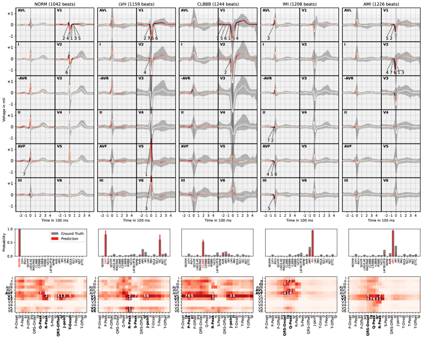
Figure 13: Results of the glocal (dataset-wide) analysis for the saliency as attribution method and LeNet as model architecture (analogous to Fig. 4).

A.5 XAI methods

In order to make the paper self-contained, we provide short technical descriptions of the XAI methods used in this study. For more details, we refer the reader to the original publications.

With TCAV [35] it is possible to test a trained model against human comprehensible concepts. These concepts are implicitly defined by data. In contrast to the attribution maps, with TCAV we can explicitly determine, whether e.g. a high magnitude at the R-Peak of a signal is of high importance for the prediction of a certain pathology. In general, the TCAV approach works as follows. First, a binary data set is compiled per concept, where the concept occurs in the positive samples and the negative samples represent a random composition of data points in which the concept does not occur. Second, for every dataset, we train a linear classifier that tries to differentiate the positive samples from the negative samples in feature space. The orthogonal vector of the linear classifier is called concept activation vector (CAV). It provides the direction in which the concept lies in the feature space, as depicted in Figure 14. Using the CAV, we can determine the TCAV score. First, we calculate for every data point $x_{i}$ belonging to class k the sensitivity $S_{C,k,l}(x_{i})$ which constitutes the directional derivative of a class k in the direction of the CAV $v_{C}^{l}$ :

$$\begin{split}S_{C,k,l}(x_{i})&=\frac{\partial h_{l,k}(x_{i})}{\partial v_{C}^{l}}\\ &=\nabla h_{l,k}(f_{l}(x_{i}))*v_{C}^{l},\end{split}$$ (1)

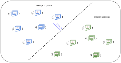
Figure 14: The concept activation vector ($v_{l}^{C}$) of concept $C$ at layer $l$ is a vector orthogonal to the classifier’s decision boundary, which differentiates data points in which the concept occurs from random negative samples. All data points are projected into the feature space of layer $l$ of the given model. In other words, the linear classifier learns to detect for a data sample, whether the given concept C is present in the feature space at layer $l$ of the model.

In a second step, the TCAV score is built as the fraction of data points $x_{i}$ that belong to class $k$, that have a positive sensitivity $S_{C,k,l}(x_{i})$:

$$TCAV_{C,k,l}=\frac{\lvert\{x\in X_{k}:S_{C,k,l}(x)>0\}\rvert}{\lvert X_{k}\rvert}$$ (2)

It provides a global score that allows assessing the importance of concept $C$ at layer $l$ of the model for the prediction of class $k$.

Saliency maps [29] infer attribution simply from input gradients of the corresponding class outputs. Denoting the model’s output logits for class $k$ by $F_{k}(x)$, the saliency for input sample $x$, we define saliency maps as [29]

$$S_{k}(x)=\left|\frac{\partial F_{k}}{\partial x}\right|$$ (3)

GradCAM [23] takes a different approach in that it does not use the gradient information directly as attribution maps, but rather to calculate weights for the activation feature maps. To this end, on a given convolutional layer, for every $K$ feature maps, it computes the activation gradient $\frac{\delta y^{c}}{\delta A^{k}}$ of the class $c$ we try to explain. Then, it calculates for every feature map $A^{k}$ a weight $\alpha^{k}$ by simply applying a global mean pooling to the gradient:

$$\alpha^{k}_{c}=\frac{1}{Z}\sum_{i}\sum_{j}\frac{\delta y^{c}}{\delta A^{k}_{i,j}}\,,$$ (4)

where $Z$ corresponds to the number of entries in the feature map. The attribution map is then given by the ReLU activation of a weighted mean of the feature maps:

$$G=\text{ReLU}(\frac{1}{K}\sum_{k}\alpha^{k}_{c}A^{k})$$ (5)

Layer-wise relevance propagation (LRP) [40] propagates the model prediction $f(x)$ from output to input, assigning attributions to each neuron in the network, which are computed based on activations and weights of the same layer and attributions of connected neurons. A key idea of the method is that attributions are conserved across layers, i.e., the sum of the attributions at each layer $k$ yields the model prediction $f(x)$:

$$\sum_{i}R^{k}_{i}=f(x)$$ (6)

The exact update procedure is dependent on the rule that is used. We use the $\epsilon$-rule for all layers, which is formally equivalent to taking the product of input and input gradient (Gradient * Input) for models with only ReLU activations [59] as those considered in this work:

$$R_{j}=\sum_{k}\frac{a_{j}w_{jk}}{\epsilon\sum_{j}{a_{j}w_{jk}}}R_{k}$$ (7)

We also tested the Z-Plus rule for convolutional layers, which represents a default choice in the imaging domain:

$$R_{j}=\sum_{k}\frac{z_{jk}^{+}}{\sum_{k}{z_{jk}^{+}}}R_{k}$$ (8)

with $z_{jk}^{+}=x_{j}w_{jk}^{+}$ and $w_{jk}^{+}=1_{w_{jk\geq 0}}w_{jk}$. Due to worse results in the sanity check, we omit this rule and use the $\epsilon$-rule throughout the model.

Integrated Gradients (IG) [41] is a model-agnostic explainability method that computes attribution maps by integrating over multiple gradients. It starts with a baseline $\boldsymbol{b}$, which is chosen as an input with neutral prediction, e.g. a null tensor, which would in our case represent an ECG with no electrical activity. To explain the prediction of class $k$ for a given input ECG $x\in\mathbb{R}^{m\times n}$, IG integrates the gradients of the model prediction for class $k$ w.r.t to all interpolated data points between the baseline $\boldsymbol{b}$ and $\boldsymbol{x}$:

$$IG_{k,i}(\boldsymbol{x})=(x_{i}-b_{i})\times\int_{0}^{1}\frac{\partial F_{k}(\boldsymbol{b}+\alpha\times(\boldsymbol{x}-\boldsymbol{b}))}{\partial x_{i}}d\alpha$$ (9)

where $F_{k}(\boldsymbol{x})$ is the logit for a data point $\boldsymbol{x}$ for class $k$ and $IG_{k,i,j}(\boldsymbol{x})$ the explanation of class $k$ for the $i$-th timestep in input $\boldsymbol{x}$. The full explanation is then given by: $IG_{k}(\boldsymbol{x})$, which is also called attribution map. It assigns an attribution score to each timestep $i$ in the input $\boldsymbol{x}$. By superimposing the attribution map on the ECG, we can mark the relevant areas in the ECG and thus simplify the interpretation of the diagnosis.

References

- [1] CDC, “National Ambulatory Medical Care Survey: 2016 National Summary Tables,” tech. rep., Centers for Disease Control and Prevention, 2019.
- [2] J. Schläpfer and H. J. Wellens, “Computer-interpreted electrocardiograms: benefits and limitations,” Journal of the American College of Cardiology, vol. 70, no. 9, pp. 1183–1192, 2017.
- [3] E. J. Topol, “What’s lurking in your electrocardiogram?,” The Lancet, vol. 397, no. 10276, p. 785, 2021.
- [4] N. Strodthoff and C. Strodthoff, “Detecting and interpreting myocardial infarction using fully convolutional neural networks,” Physiological Measurement, vol. 40, p. 015001, jan 2019.
- [5] N. Strodthoff, P. Wagner, T. Schaeffter, and W. Samek, “Deep learning for ECG analysis: Benchmarks and insights from PTB-XL,” IEEE Journal of Biomedical and Health Informatics, pp. 1–1, 2020.
- [6] A. H. Kashou, W.-Y. Ko, Z. I. Attia, M. S. Cohen, P. A. Friedman, and P. A. Noseworthy, “A comprehensive artificial intelligence–enabled electrocardiogram interpretation program,” Cardiovascular Digital Health Journal, vol. 1, pp. 62–70, Sept. 2020.
- [7] A. Y. Hannun, P. Rajpurkar, M. Haghpanahi, G. H. Tison, C. Bourn, M. P. Turakhia, and A. Y. Ng, “Cardiologist-level arrhythmia detection and classification in ambulatory electrocardiograms using a deep neural network,” Nature Medicine, vol. 25, pp. 65–69, Jan. 2019.
- [8] G. H. Tison, J. Zhang, F. N. Delling, and R. C. Deo, “Automated and interpretable patient ECG profiles for disease detection, tracking, and discovery,” Circulation: Cardiovascular Quality and Outcomes, vol. 12, Sept. 2019.
- [9] Z. I. Attia, P. A. Friedman, P. A. Noseworthy, F. Lopez-Jimenez, D. J. Ladewig, G. Satam, P. A. Pellikka, T. M. Munger, S. J. Asirvatham, C. G. Scott, R. E. Carter, and S. Kapa, “Age and sex estimation using artificial intelligence from standard 12-lead ECGs,” Circulation: Arrhythmia and Electrophysiology, vol. 12, Sept. 2019.
- [10] Z. I. Attia, S. Kapa, F. Lopez-Jimenez, P. M. McKie, D. J. Ladewig, G. Satam, P. A. Pellikka, M. Enriquez-Sarano, P. A. Noseworthy, T. M. Munger, S. J. Asirvatham, C. G. Scott, R. E. Carter, and P. A. Friedman, “Screening for cardiac contractile dysfunction using an artificial intelligence–enabled electrocardiogram,” Nature Medicine, vol. 25, pp. 70–74, Jan. 2019.
- [11] Z. I. Attia, P. A. Noseworthy, F. Lopez-Jimenez, S. J. Asirvatham, A. J. Deshmukh, B. J. Gersh, R. E. Carter, X. Yao, A. A. Rabinstein, B. J. Erickson, et al., “An artificial intelligence-enabled ecg algorithm for the identification of patients with atrial fibrillation during sinus rhythm: a retrospective analysis of outcome prediction,” The Lancet, vol. 394, no. 10201, pp. 861–867, 2019.
- [12] J. myoung Kwon, Y. Cho, K.-H. Jeon, S. Cho, K.-H. Kim, S. D. Baek, S. Jeung, J. Park, and B.-H. Oh, “A deep learning algorithm to detect anaemia with ECGs: a retrospective, multicentre study,” The Lancet Digital Health, vol. 2, pp. e358–e367, July 2020.
- [13] A. R. Kulkarni, A. A. Patel, K. V. Pipal, S. G. Jaiswal, M. T. Jaisinghani, V. Thulkar, L. Gajbhiye, P. Gondane, A. B. Patel, M. Mamtani, and H. Kulkarni, “Machine-learning algorithm to non-invasively detect diabetes and pre-diabetes from electrocardiogram,” BMJ Innovations, 2022.
- [14] J. C. Ahn, Z. I. Attia, P. Rattan, A. F. Mullan, S. Buryska, A. M. Allen, P. S. Kamath, P. A. Friedman, V. H. Shah, P. A. Noseworthy, and D. A. Simonetto, “Development of the AI-cirrhosis-ECG score: An electrocardiogram-based deep learning model in cirrhosis,” American Journal of Gastroenterology, vol. 117, pp. 424–432, Dec. 2021.
- [15] I. Covert, S. Lundberg, and S.-I. Lee, “Explaining by removing: A unified framework for model explanation,” Journal of Machine Learning Research, vol. 22, no. 209, pp. 1–90, 2021.
- [16] S. M. Lundberg and S.-I. Lee, “A unified approach to interpreting model predictions,” Advances in Neural Information Processing Systems, vol. 30, 2017.
- [17] W. Samek, G. Montavon, S. Lapuschkin, C. J. Anders, and K.-R. Müller, “Explaining deep neural networks and beyond: A review of methods and applications,” Proceedings of the IEEE, vol. 109, no. 3, pp. 247–278, 2021.
- [18] A. Saporta, X. Gui, A. Agrawal, A. Pareek, S. Q. Truong, C. D. Nguyen, V.-D. Ngo, J. Seekins, F. G. Blankenberg, A. Y. Ng, et al., “Benchmarking saliency methods for chest x-ray interpretation,” Nature Machine Intelligence, vol. 4, no. 10, pp. 867–878, 2022.
- [19] A. J. DeGrave, J. D. Janizek, and S.-I. Lee, “AI for radiographic COVID-19 detection selects shortcuts over signal,” Nature Machine Intelligence, vol. 3, pp. 610–619, May 2021.
- [20] Y. M. Ayano, F. Schwenker, B. D. Dufera, and T. G. Debelee, “Interpretable machine learning techniques in ECG-based heart disease classification: A systematic review,” Diagnostics, vol. 13, p. 111, Dec. 2022.
- [21] Q. Yao, R. Wang, X. Fan, J. Liu, and Y. Li, “Multi-class arrhythmia detection from 12-lead varied-length ecg using attention-based time-incremental convolutional neural network,” Information Fusion, vol. 53, pp. 174–182, 2020.
- [22] Y. Elul, A. A. Rosenberg, A. Schuster, A. M. Bronstein, and Y. Yaniv, “Meeting the unmet needs of clinicians from AI systems showcased for cardiology with deep-learning–based ECG analysis,” Proceedings of the National Academy of Sciences, vol. 118, June 2021.
- [23] R. R. Selvaraju, M. Cogswell, A. Das, R. Vedantam, D. Parikh, and D. Batra, “Grad-CAM: Visual explanations from deep networks via gradient-based localization,” International Journal of Computer Vision, vol. 128, pp. 336–359, Oct. 2019.
- [24] S. Raghunath, A. E. U. Cerna, L. Jing, D. P. vanMaanen, J. Stough, D. N. Hartzel, J. B. Leader, H. L. Kirchner, M. C. Stumpe, A. Hafez, A. Nemani, T. Carbonati, K. W. Johnson, K. Young, C. W. Good, J. M. Pfeifer, A. A. Patel, B. P. Delisle, A. Alsaid, D. Beer, C. M. Haggerty, and B. K. Fornwalt, “Prediction of mortality from 12-lead electrocardiogram voltage data using a deep neural network,” Nature Medicine, vol. 26, pp. 886–891, May 2020.
- [25] R. R. van de Leur, K. Taha, M. N. Bos, J. F. van der Heijden, D. Gupta, M. J. Cramer, R. J. Hassink, P. van der Harst, P. A. Doevendans, F. W. Asselbergs, et al., “Discovering and visualizing disease-specific electrocardiogram features using deep learning: proof-of-concept in phospholamban gene mutation carriers,” Circulation: Arrhythmia and Electrophysiology, vol. 14, no. 2, p. e009056, 2021.
- [26] S. D. Goodfellow, A. Goodwin, R. Greer, P. C. Laussen, M. Mazwi, and D. Eytan, “Towards understanding ecg rhythm classification using convolutional neural networks and attention mappings,” in Machine learning for healthcare conference, pp. 83–101, PMLR, 2018.
- [27] S. A. Hicks, J. L. Isaksen, V. Thambawita, J. Ghouse, G. Ahlberg, A. Linneberg, N. Grarup, I. Strümke, C. Ellervik, M. S. Olesen, et al., “Explaining deep neural networks for knowledge discovery in electrocardiogram analysis,” Scientific reports, vol. 11, no. 1, pp. 1–11, 2021.
- [28] L. Lu, T. Zhu, A. H. Ribeiro, L. Clifton, E. Zhao, A. L. P. Ribeiro, Y.-T. Zhang, and D. A. Clifton, “Knowledge discovery with electrocardiography using interpretable deep neural networks,” medRxiv, 2022.
- [29] K. Simonyan, A. Vedaldi, and A. Zisserman, “Deep inside convolutional networks: Visualising image classification models and saliency maps,” arXiv preprint arXiv:1312.6034, 2013.
- [30] J.-M. Kwon, S. Y. Lee, K.-H. Jeon, Y. Lee, K.-H. Kim, J. Park, B.-H. Oh, and M.-M. Lee, “Deep learning–based algorithm for detecting aortic stenosis using electrocardiography,” Journal of the American Heart Association, vol. 9, no. 7, p. e014717, 2020.
- [31] Y. Jones, F. Deligianni, and J. Dalton, “Improving ecg classification interpretability using saliency maps,” in 2020 IEEE 20th International Conference on Bioinformatics and Bioengineering (BIBE), pp. 675–682, 2020.
- [32] E. M. Lima, A. H. Ribeiro, G. M. Paixão, M. H. Ribeiro, M. M. Pinto-Filho, P. R. Gomes, D. M. Oliveira, E. C. Sabino, B. B. Duncan, L. Giatti, et al., “Deep neural network-estimated electrocardiographic age as a mortality predictor,” Nature communications, vol. 12, no. 1, pp. 1–10, 2021.
- [33] Y. Cho, J.-m. Kwon, K.-H. Kim, J. R. Medina-Inojosa, K.-H. Jeon, S. Cho, S. Y. Lee, J. Park, and B.-H. Oh, “Artificial intelligence algorithm for detecting myocardial infarction using six-lead electrocardiography,” Scientific reports, vol. 10, no. 1, pp. 1–10, 2020.
- [34] J. W. Hughes, J. E. Olgin, R. Avram, S. A. Abreau, T. Sittler, K. Radia, H. Hsia, T. Walters, B. Lee, J. E. Gonzalez, and G. H. Tison, “Performance of a convolutional neural network and explainability technique for 12-lead electrocardiogram interpretation,” JAMA Cardiology, vol. 6, p. 1285, Nov. 2021.
- [35] B. Kim, M. Wattenberg, J. Gilmer, C. Cai, J. Wexler, F. Viegas, et al., “Interpretability beyond feature attribution: Quantitative testing with concept activation vectors (tcav),” in International conference on machine learning, pp. 2668–2677, PMLR, 2018.
- [36] T. Bender, J. M. Beinecke, D. Krefting, C. Müller, H. Dathe, T. Seidler, N. Spicher, and A.-C. Hauschild, “Analysis of a deep learning model for 12-lead ecg classification reveals learned features similar to diagnostic criteria,” arXiv preprint arXiv:2211.01738, 2022.
- [37] P. Wagner, N. Strodthoff, R.-D. Bousseljot, D. Kreiseler, F. I. Lunze, W. Samek, and T. Schaeffter, “PTB-XL, a large publicly available electrocardiography dataset,” Scientific Data, vol. 7, no. 1, p. 154, 2020.
- [38] P. Wagner, N. Strodthoff, R.-D. Bousseljot, W. Samek, and T. Schaeffter, “PTB-XL, a large publicly available electrocardiography dataset,” 2020.
- [39] A. L. Goldberger, L. A. N. Amaral, L. Glass, J. M. Hausdorff, P. C. Ivanov, R. G. Mark, J. E. Mietus, G. B. Moody, C.-K. Peng, and H. E. Stanley, “PhysioBank, PhysioToolkit, and PhysioNet,” Circulation, vol. 101, no. 23, pp. e215–e220, 2000.
- [40] S. Bach, A. Binder, G. Montavon, F. Klauschen, K.-R. Müller, and W. Samek, “On pixel-wise explanations for non-linear classifier decisions by layer-wise relevance propagation,” PLOS ONE, vol. 10, p. e0130140, July 2015.
- [41] M. Sundararajan, A. Taly, and Q. Yan, “Axiomatic attribution for deep networks,” in International Conference on Machine Learning, pp. 3319–3328, PMLR, 2017.
- [42] S. Krishna, T. Han, A. Gu, J. Pombra, S. Jabbari, S. Wu, and H. Lakkaraju, “The disagreement problem in explainable machine learning: A practitioner’s perspective,” arXiv preprint arXiv:2202.01602, 2022.
- [43] B. Surawicz, R. Childers, B. J. Deal, and L. S. Gettes, “Aha/accf/hrs recommendations for the standardization and interpretation of the electrocardiogram: part iii: intraventricular conduction disturbances a scientific statement from the american heart association electrocardiography and arrhythmias committee, council on clinical cardiology; the american college of cardiology foundation; and the heart rhythm society endorsed by the international society for computerized electrocardiology,” Journal of the American College of Cardiology, vol. 53, no. 11, pp. 976–981, 2009.
- [44] M. Sokolow and T. P. Lyon, “The ventricular complex in left ventricular hypertrophy as obtained by unipolar precordial and limb leads,” American heart journal, vol. 37, no. 2, pp. 161–186, 1949.
- [45] K. Thygesen, J. S. Alpert, A. S. Jaffe, B. R. Chaitman, J. J. Bax, D. A. Morrow, H. D. White, and E. G. on behalf of the Joint European Society of Cardiology (ESC)/American College of Cardiology (ACC)/American Heart Association (AHA)/World Heart Federation (WHF) Task Force for the Universal Definition of Myocardial Infarction, “Fourth universal definition of myocardial infarction (2018),” Journal of the American College of Cardiology, vol. 72, no. 18, pp. 2231–2264, 2018.
- [46] N. Samesima, L. F. Azevedo, L. D. N. J. D. Matos, L. S. Echenique, C. E. Negrao, and C. A. Pastore, “Comparison of electrocardiographic criteria for identifying left ventricular hypertrophy in athletes from different sports modalities,” Clinics, vol. 72, no. 6, pp. 343–350, 2017.
- [47] M. H. Nikoo, A. Aslani, and M. V. Jorat, “Lbbb: state-of-the-art criteria,” International Cardiovascular Research Journal, 2013.
- [48] P. Rautaharju and F. Rautaharju, Investigative electrocardiography in epidemiological studies and clinical trials. Springer Science & Business Media, 2007.
- [49] L. Seyyed-Kalantari, H. Zhang, M. B. A. McDermott, I. Y. Chen, and M. Ghassemi, “Underdiagnosis bias of artificial intelligence algorithms applied to chest radiographs in under-served patient populations,” Nature Medicine, vol. 27, pp. 2176–2182, Dec. 2021.
- [50] S. Lapuschkin, S. Wäldchen, A. Binder, G. Montavon, W. Samek, and K.-R. Müller, “Unmasking clever hans predictors and assessing what machines really learn,” Nature communications, vol. 10, no. 1, pp. 1–8, 2019.
- [51] J. Vielhaben, S. Blücher, and N. Strodthoff, “Multi-dimensional concept discovery (mcd): A unifying framework with completeness guarantees,” arXiv preprint arXiv:2301.11911, 2023.
- [52] P. Macfarlane, B. Devine, and E. Clark, “The university of Glasgow (Uni-G) ECG analysis program,” in Computers in Cardiology, 2005, pp. 451–454, 2005.
- [53] A. H. Ribeiro, M. H. Ribeiro, G. M. M. Paixão, D. M. Oliveira, P. R. Gomes, J. A. Canazart, M. P. S. Ferreira, C. R. Andersson, P. W. Macfarlane, W. Meira, T. B. Schön, and A. L. P. Ribeiro, “Automatic diagnosis of the 12-lead ECG using a deep neural network,” Nature Communications, vol. 11, Apr. 2020.
- [54] T. Mehari and N. Strodthoff, “Self-supervised representation learning from 12-lead ECG data,” Computers in Biology and Medicine, vol. 141, p. 105114, 2022.
- [55] T. Mehari and N. Strodthoff, “Advancing the state-of-the-art for ecg analysis through structured state space models,” arXiv preprint arXiv:2211.07579, 2022. Extended abstract Machine Learning for Health 2022.
- [56] Y. LeCun, B. Boser, J. S. Denker, D. Henderson, R. E. Howard, W. Hubbard, and L. D. Jackel, “Backpropagation applied to handwritten zip code recognition,” Neural computation, vol. 1, no. 4, pp. 541–551, 1989.
- [57] K. He, X. Zhang, S. Ren, and J. Sun, “Deep residual learning for image recognition,” in Proceedings of the IEEE conference on computer vision and pattern recognition, pp. 770–778, 2016.
- [58] T. He, Z. Zhang, H. Zhang, Z. Zhang, J. Xie, and M. Li, “Bag of tricks for image classification with convolutional neural networks,” in Proceedings of the IEEE Conference on Computer Vision and Pattern Recognition, pp. 558–567, 2019.
- [59] M. Ancona, E. Ceolini, C. Öztireli, and M. Gross, “Towards better understanding of gradient-based attribution methods for deep neural networks,” in International Conference on Learning Representations, 2018.
- [60] N. Pilia, C. Nagel, G. Lenis, S. Becker, O. Dössel, and A. Loewe, “ECGdeli - an open source ECG delineation toolbox for MATLAB,” SoftwareX, vol. 13, p. 100639, Jan. 2021.
- [61] O. Ronneberger, P. Fischer, and T. Brox, “U-net: Convolutional networks for biomedical image segmentation,” in International Conference on Medical image computing and computer-assisted intervention, pp. 234–241, Springer, 2015.
- [62] N. Strodthoff, T. Mehari, C. Nagel, P. J. Aston, A. Sundar, C. Graff, J. K. Kanters, W. Haverkamp, O. Dössel, A. Loewe, M. Bär, and T. Schaeffter, “PTB-XL+, a comprehensive electrocardiographic feature dataset,” Scientific Data, 2023. awaiting publication.
- [63] P. Wagner, T. Mehari, W. Haverkamp, and N. Strodthoff, “PTB-XL (v1.0.1) Soft Segmentations (Delineation),” Feb. 2023.
- [64] N. Kokhlikyan, V. Miglani, M. Martin, E. Wang, J. Reynolds, A. Melnikov, N. Lunova, and O. Reblitz-Richardson, “Pytorch captum.” https://github.com/pytorch/captum, 2019.
- [65] C. J. Anders, D. Neumann, W. Samek, K.-R. Müller, and S. Lapuschkin, “Software for dataset-wide xai: From local explanations to global insights with Zennit, CoRelAy, and ViRelAy,” arxiv preprint arxiv:2106.13200, 2021.
- [66] T. Lewis, Heart, ch. 5, pp. 367–402. Shaw, 1914.
- [67] D. W. Romhilt, K. E. Bove, R. J. Norris, E. Conyers, S. Conrada, D. T. Rowlands, and R. C. Scott, “A critical appraisal of the electrocardiographic criteria for the diagnosis of left ventricular hypertrophy,” Circulation, vol. 40, pp. 185–196, Aug. 1969.