DistriBlock: Identifying adversarial audio samples by leveraging characteristics of the output distribution

Abstract

Adversarial attacks can mislead automatic speech recognition (ASR) systems into predicting an arbitrary target text, thus posing a clear security threat. To prevent such attacks, we propose DistriBlock, an efficient detection strategy applicable to any ASR system that predicts a probability distribution over output tokens in each time step. We measure a set of characteristics of this distribution: the median, maximum, and minimum over the output probabilities, the entropy of the distribution, as well as the Kullback-Leibler and the Jensen-Shannon divergence with respect to the distributions of the subsequent time step. Then, by leveraging the characteristics observed for both benign and adversarial data, we apply binary classifiers, including simple threshold-based classification, ensembles of such classifiers, and neural networks. Through extensive analysis across different state-of-the-art ASR systems and language data sets, we demonstrate the supreme performance of this approach, with a mean area under the receiver operating characteristic for distinguishing target adversarial examples against clean and noisy data of 99% and 97%, respectively. To assess the robustness of our method, we show that adaptive adversarial examples that can circumvent DistriBlock are much noisier, which makes them easier to detect through filtering and creates another avenue for preserving the system’s robustness.

1 Introduction

Voice recognition technologies are widely used in the devices that we interact with daily—in smartphones or virtual assistants—and are also being adapted for more safety-critical tasks like self-driving cars [46] and healthcare applications. Safeguarding these systems from malicious attacks thus plays a more and more critical role, since manipulated erroneous transcriptions can potentially lead to severe security harms.

Figure 1: Proposed workflow to identify AEs: (1) compute output probability distribution characteristics per time step, (2) use a detector to tell benign data and AEs apart. $c^{1}$ to $c^{T}$ represent input characteristics, while $s^{c}$ denotes final scores.

State-of-the-art automated speech recognition systems are based on deep learning [20, 11, 9, 34]. Unfortunately, deep neural networks (NNs) are highly vulnerable to adversarial attacks, since the inherent properties of the model make it easy to generate inputs—referred to as adversarial examples (AEs)—that are necessarily mislabeled, simply by incorporating a low-level additive perturbation [41, 15, 19, 12]. A well-established method to generate AEs also applicable to ASR systems, is the Carlini & Wagner (C&W) attack [7]. It aims to minimize a perturbation $\delta$ that—when added to a benign audio signal x—induces the system to recognize a phrase chosen by the attacker. Moreover, attacks specifically developed for ASR systems shape the perturbations to fall below the estimated time-frequency masking threshold of human listeners, rendering $\delta$ hardly perceptible, and sometimes even inaudible to humans [39, 33]. This underlines the urgent need for approaches to automatically detect AE attacks on ASR systems.

Motivated by the intuition that attacks may result in a higher prediction uncertainty displayed by the ASR system, we develop a novel detection technique that allows to efficiently distinguish adversarial from benign audio signals and can be used for any ASR system that estimates a probability distribution over tokens at each step of generating the output sequence—which is the case for the vast majority of state-of-the-art systems. More precisely, our contributions are as follows:

1. We propose DistriBlock: binary classifiers that build on characteristics of the probability distribution over tokens, which can be interpreted as a simple proxy of the prediction uncertainty of the ASR system.

2. We perform an extensive empirical analysis across diverse state-of-the-art ASR models, attack types, and datasets covering a range of languages, that demonstrate the superiority of DistriBlock over previous detection methods.

3. We propose adaptive attacks specifically designed to counteract DistriBlock, but show that the resulting adversarial examples contain a higher level of noise, which makes them easier to spot for human ears and identifiable using filtering techniques.

2 Related work

When it comes to mitigating the impact of adversarial attacks, there are two main research directions. On the one hand, there is a strand of research dedicated to enhancing the robustness of models. On the other hand, there is a separate research direction that focuses on designing detection mechanisms to recognize the presence of adversarial attacks.

Concerning the robustness of models, there are diverse strategies, one of which involves modifying the input data within the ASR system. This concept has been adapted from the visual to the auditory domain. Examples of input data modifications include quantization, temporal smoothing, down-sampling, low-pass filtering, slow feature analysis, and auto-encoder reformation [24, 18, 31]. However, these techniques become less effective once integrated into the attacker’s deep learning framework [48]. Another strategy to mitigate adversarial attacks is to accept their existence and force them to be perceivable by humans [14], with the drawback that the AEs can continue misleading the system. Adversarial training [23], in contrast, involves employing AEs during training to enhance the NN’s resiliency against adversarial attacks. Due to the impracticality of covering all potential attack classes through training, adversarial training has major limitations when applied to large and complex data sets, such as those commonly used in speech research [51]. Additionally, this approach demands high computational costs and can result in reducing the accuracy of benign data. A recent method borrowed from the field of image recognition is adversarial purification, where generative models are employed to cleanse the input data prior to inference [49, 28]. However, only a few studies have investigated this strategy within the realm of audio. Presently, its ASR applications are confined to smaller vocabularies, and it necessitates substantial computational resources, while also resulting in decreased accuracy when applied to benign data [47].

In the context of improving the discriminative power against adversarial attacks, [35] introduced a noise flooding (NF) detector method that quantifies the random noise needed to change the model’s prediction, with smaller levels observed for AEs. Subsequently, they leverage this information to build binary classifiers. However, NF was only tested against a genetic untargeted attack on a 10-word speech classification system. A prominent non-differentiable approach uses the inherent temporal dependency (TD) in raw audio signals [48]. This strategy requires a minimal length of the audio stream for optimal performance. Unfortunately, [50] successfully evaded the detection mechanism of TD by preserving the necessary temporal correlations, leading to the generation of robust AEs once again. [13] proposed AEs detection based on uncertainty measures for hybrid ASR systems that utilize stochastic NNs. They applied their method to a limited vocabulary tailored for digit recognition. One of these uncertainty metrics—the mean-entropy—is also among those characteristics of the output distribution that we investigate, next to many others, for constructing defenses against AEs in this paper. It’s worth noting that [26] also utilized the averaged Kullback Leibler divergence between the output distributions of consecutive time steps (which they referred to as mean temporal distance), but to monitor the performance of ASR systems in noisy multi-channel environments.

3 Background

Adversarial attacks

Let $f(\cdot)$ be the ASR system’s function, that maps an audio input to the sequence of words it most likely contains. Moreover, let $x$ be an audio signal with label transcript $y$ that is correctly predicted by the ASR, i.e., $y=f(x)$. A targeted AE can be created by finding a small perturbation $\delta$ that causes the ASR system to predict a desired transcript $\hat{y}$ given $x+\delta$, i.e., $f(x+\delta)=\hat{y}\neq y=f(x).$ This perturbation $\delta$ is usually estimated by gradient descent-based minimization of the following function

$$l(x,\delta,\hat{y})=l_{t}(f(x+\delta),\hat{y})+c\cdot l_{a}(x,\delta)\enspace,$$ (1)

which includes two loss functions: (1) a task-specific loss, $l_{t}(\cdot)$, to find a distortion that induces the model to output the desired transcription target $\hat{y}$, and (2) an acoustic loss, $l_{a}(\cdot)$, that is used to make the noise $\delta$ smaller in energy and/or imperceptible to human listeners. In the initial steps of the iterative optimization procedure, the weighting parameter c is usually set to small values to first find a viable AE. Later, c is often increased, in order to minimize the distortion, to render it as inconspicuous as possible.

The most prominent targeted attacks for audio are the C&W Attack and the Imperceptible also known as Psychoacoustic Attack, two well-established optimization-based adversarial algorithms. In the C&W attack [7], $l_{t}$ is the negative log-likelihood of the target phrase and $l_{a}=|\delta|_{2}^{2}$. Moreover, $|\delta|$ is constrained to be smaller than a predefined value $\epsilon$, which is decreased step-wise in an iterative process. The Psychoacoustic Attack [39, 33] is divided into two stages. The first stage of the attack follows the approach outlined by C&W. The second stage of the algorithm aims to decrease the perceptibility of the noise by using frequency masking, following psychoacoustic principles. For untargeted adversarial attacks, the objective is to prevent models from predicting the correct output but no specific target transcription is given. Several untargeted attacks on ASR systems have been proposed. These include the projected gradient descent (PGD) [23], a well-known general attack method, as well as two black-box attacks—the Kenansville attack [2, 1] utilizing signal processing methods to discard certain frequency components, and the genetic attack [3] that results from a gradient-free optimization algorithm.

End-to-end ASR systems

An E2E ASR system [32] can be described as a unified ASR model that directly transcribes a speech waveform into text, as opposed to orchestrating a pipeline of separate ASR components. In general terms, the input of the system is a series of acoustic features extracted from overlapping speech frames. The model processes this series of acoustic features and predicts a probability distribution over tokens (e.g., phonemes, characters, or sub-word units) in each time step. Subsequently, utilizing a decoding and alignment algorithm, it determines the output text. Ideally, E2E ASR models are fully differentiable and thus can be trained end-to-end by maximizing the conditional log-likelihood with respect to the desired output. Various E2E ASR models follow an encoder-only or an encoder-decoder architecture and typically are built using recurrent neural network (RNN) or transformer layers. Special care is taken of the unknown temporal alignments between the input waveform and output text, where the alignment can be modeled explicitly (e.g., CTC [17], RNN-T [16]), or implicitly using attention [44]. Furthermore, language models can be integrated to improve prediction accuracy by considering the most probable sequences [42].

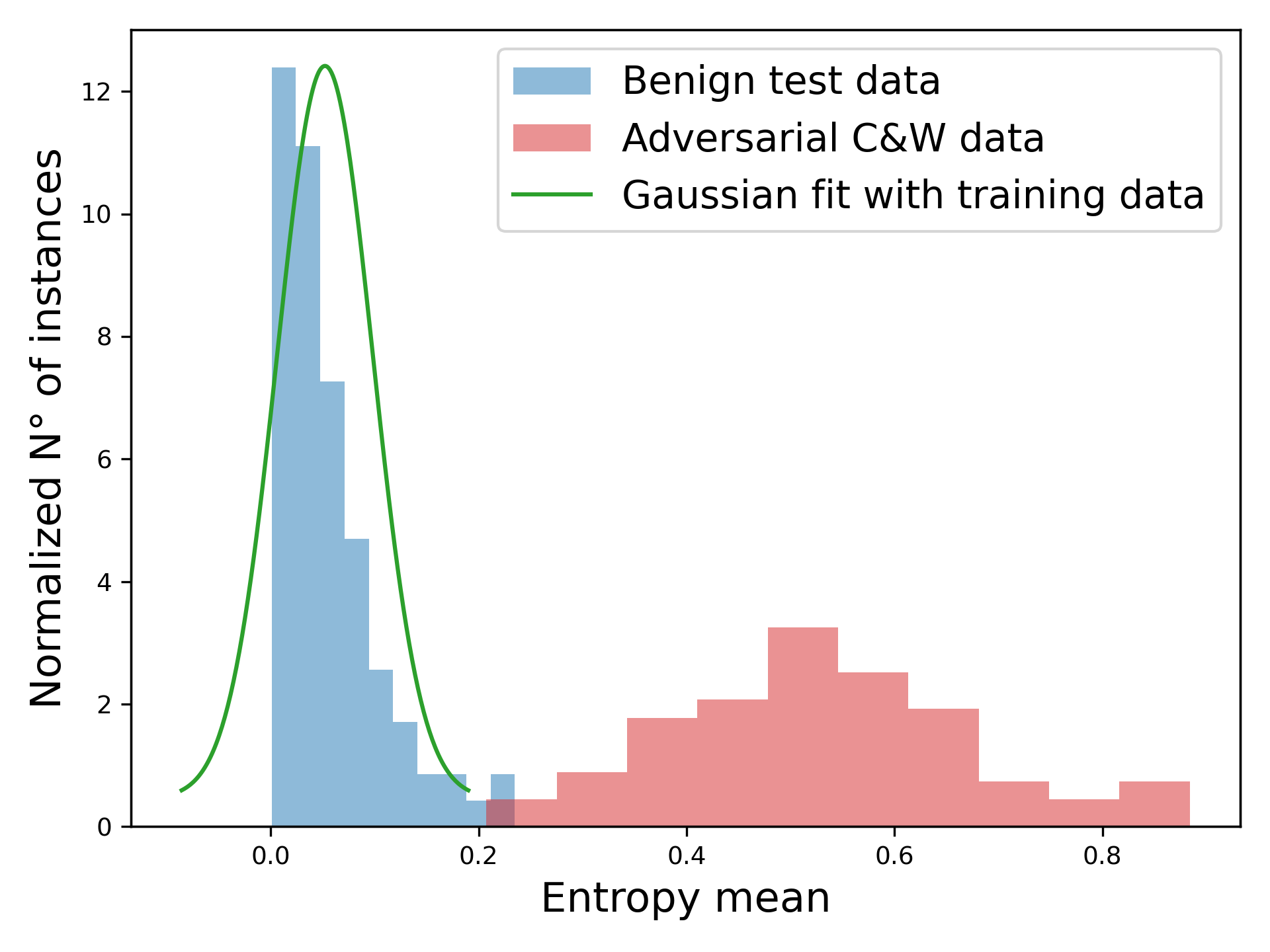
(a) Benign test-clean data vs.
C&W AEs.

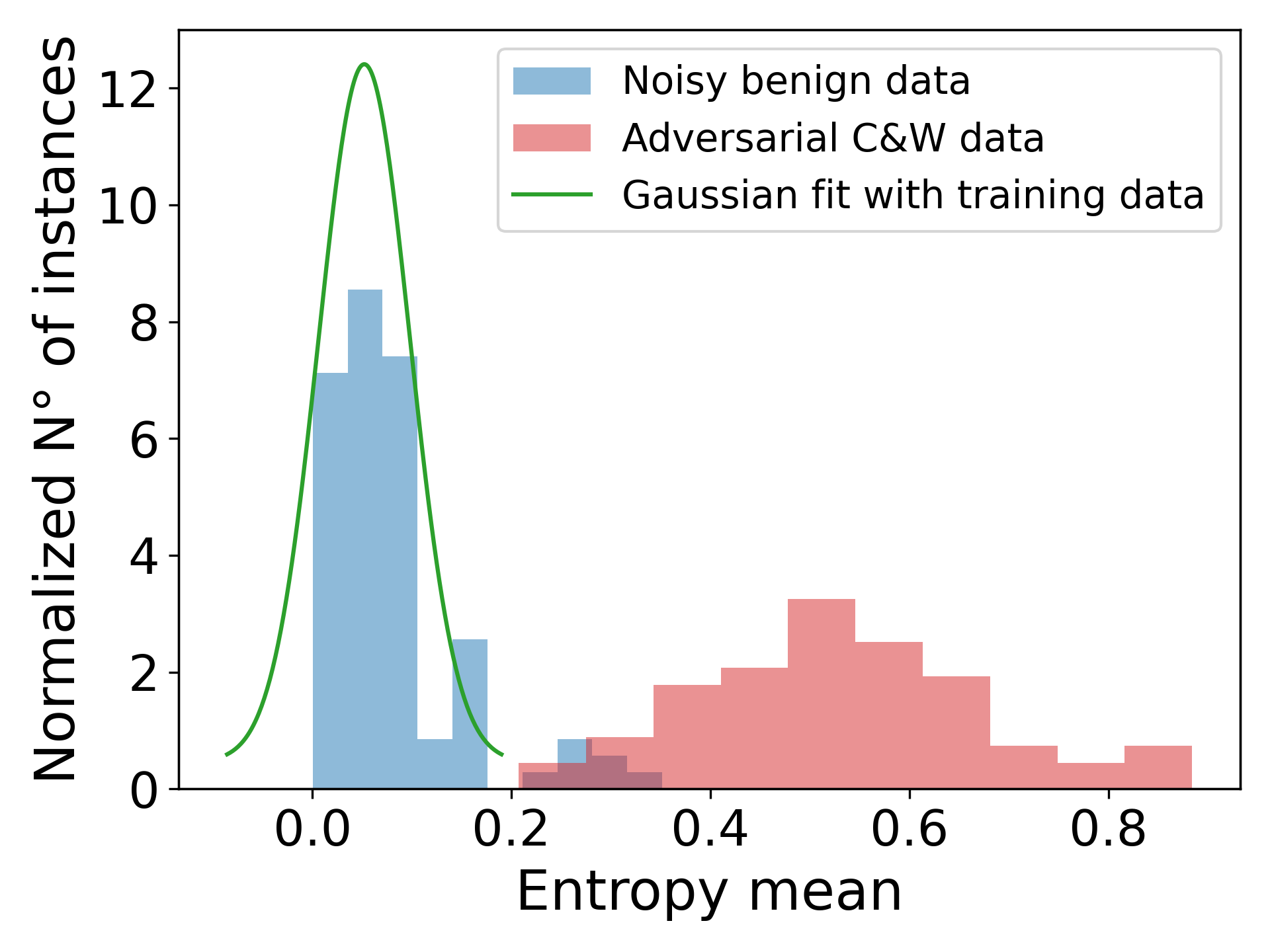
(b) Noisy benign data vs.
C&W AEs.

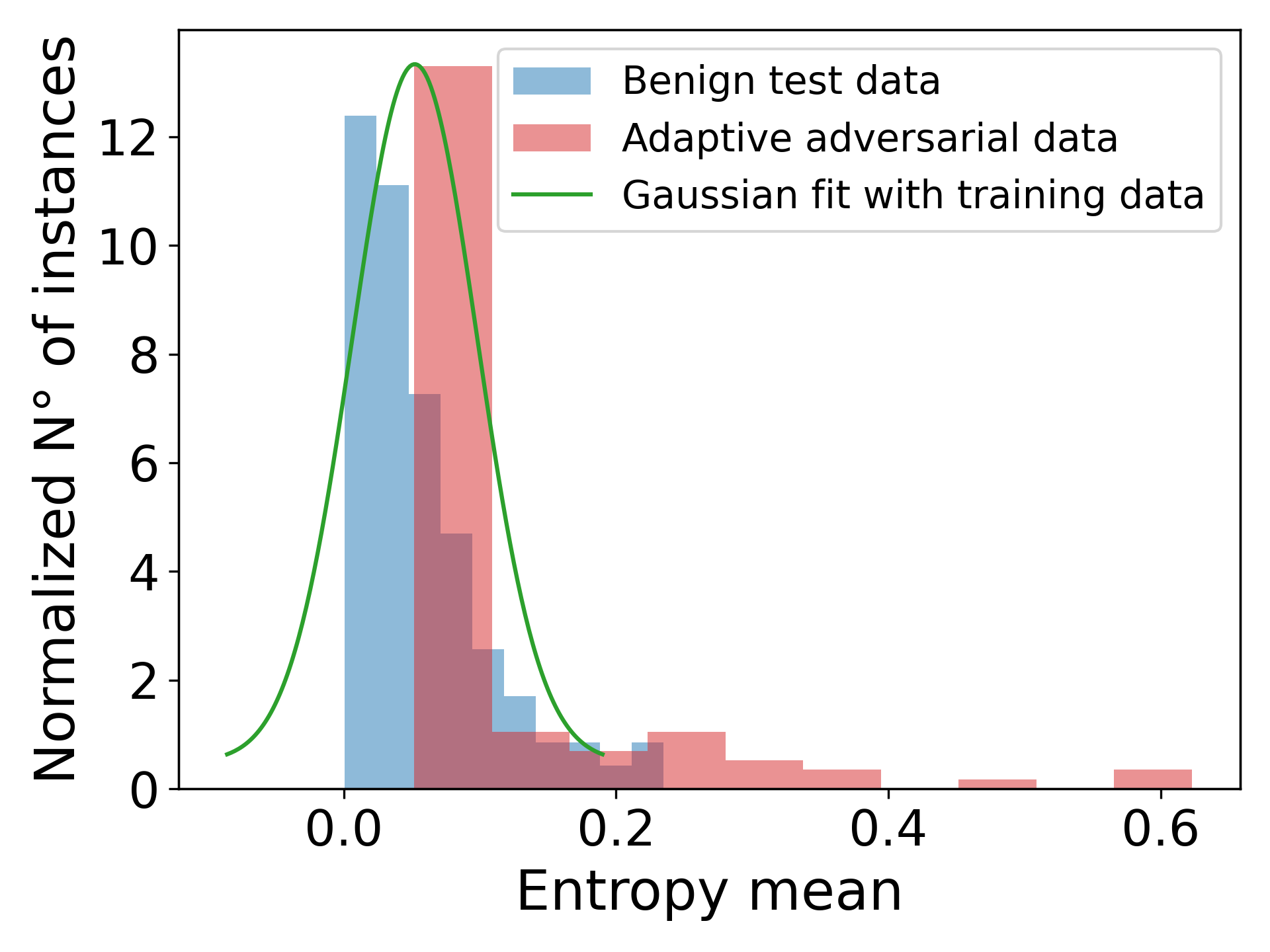
(c) Benign test-clean data vs. adaptive
C&W AEs.

Figure 2: Histograms of the mean-entropy of the LSTM model’s predictive distribution for 100 benign test samples vs. 100 C&W AEs.

4 Detecting Adversarial Examples with DistriBlock

We propose to leverage the probability distribution over the tokens from the output vocabulary to quantify uncertainty in order to identify adversarial attacks. This builds on the intuition that an adversarial input may lead to an higher uncertainty displayed by the ASR system. A schematic of our approach is displayed in Fig. 1. An audio clip—either benign or malicious—is fed to the ASR system. The system then generates probability distributions over the output tokens in each time step. The third step is to compute pertinent characteristics of these output distributions, as detailed below. Then, we use the mean, median, maximum, or minimum to aggregate the values of the characteristics into a single score per utterance. Lastly, we employ a binary classifier for differentiating adversarial instances from test data samples.

Characteristics of the output distribution

We assume that for each time step $t$ the ASR system produces a probability distribution $p^{(t)}$ over the tokens $i\in\mathcal{V}$ of a given output vocabulary $\mathcal{V}$. As a first characteristic, we use a common measure to quantify the total uncertainty in the predicted distribution of each time step, namely the Shannon entropy $H(p^{(t)})=-\sum_{i=1}^{|\mathcal{V}|}p^{(t)}(i)\cdot\log p^{(t)}(i)$. Moreover, since speech is processed sequentially from overlapping frames of the audio signal, acoustic features should transition gradually in the sequence (i.e., often the same token is predicted multiple times in a row). This should be displayed by a high similarity between probability distributions of subsequent time steps. However, the additional noise added to the speech signal of AEs potentially leads to larger changes. We, therefore, access the similarity between output distributions in two successive time steps in terms of the Kullback–Leibler divergence (KLD), $D_{\text{KL}}(p^{(t)}\|p^{(t+1)})=\sum_{i=1}^{|\mathcal{V}|}p^{(t)}(i)\cdot\log\frac{p^{(t)}(i)}{p^{(t+1)}(i)}$, as well as the Jensen-Shannon divergence (JSD), $D_{\text{JS}}(p^{(t)},p^{(t+1)})=\frac{1}{2}D_{\text{KL}}(p^{(t)}\|M)+\frac{1}{2}D_{\text{KL}}(p^{(t+1)}\|M)\text{,}$ with $M=\frac{1}{2}(p^{(t)}+p^{(t+1)})$, which can be seen as a symmetrized version of the KLD. In addition, we compute simple characteristics of the distributions for every $t\in\{1,\dots,T\}$: the median of $p^{(t)}(i),i=1,2,\dots,|\mathcal{V}|$, the minimum $\min_{i\in\{1,\dots,|\mathcal{V}|\}}p^{(t)}(i)$, and the maximum $\max_{i\in\{1,\dots,|\mathcal{V}|\}}p^{(t)}(i)$. Finally, we aggregate the step-wise values of the different characteristics into a single score, respectively, by taking the mean, median, minimum, or maximum of the values for different time steps.

Binary classifier

The extracted characteristics of the output distribution can then be used as features for a binary classifier. An option to obtain simple classifiers is to fit a Gaussian distribution to each score computed for the utterances from a held-out set of benign data. If the probability of a new audio sample is below a chosen threshold, this example is classified as adversarial. For illustration, Fig. 2 displays example histograms of the mean-entropy values of the predictive distribution given benign and adversarial inputs, respectively. A more sophisticated approach is to employ ensemble models (EMs), in which multiple Gaussian distributions, fitted to a single score each, produce a unified decision by a majority vote. Another option is to construct an NN that takes all the characteristics described above as input.

Adaptive attack

An adversary with complete knowledge of the defense strategy can implement so-called adaptive attacks. We implement such attacks, to challenge the robustness of DistriBlock. For this, we construct a new loss $l_{k}$ by adding a penalty $l_{s}$ to the loss function in Equation (1), weighted with some factor $\alpha$, that is

$$l_{k}(x,\delta,\hat{y})=(1-\alpha)\cdot l(x,\delta,\hat{y})+\alpha\cdot l_{s}(x)\enspace.$$ (2)

When attacking a Gaussian classifier that is based on characteristic $c$, $l_{s}(x)$ corresponds to the $L_{1}$ norm of the difference between the mean $\overline{s}^{c}$ of the Gaussian fitted to the respective scores of benign data (resulting from aggregating $c$ over each utterance) and the score of $x$. When attacking an EM, $l_{s}$ is set to

$$l_{s}(x)=\sum_{i=1}^{I}\lvert\overline{s}^{c_{i}}-s^{c_{i}}(x)\rvert\enspace,$$

where $c_{1}\dots c_{I}$ corresponds to the characteristics used by the Gaussian classifiers of the ensemble is composed of. In the case of NNs, $l_{s}(x)$ is simply the $L_{1}$ norm, quantifying the difference between the NN’s predicted outcome (a probability value) and one (indicating the highest probability for the benign category). We also investigated other options for choosing $l_{s}$, which are described in App. A.

5 Experiments

Table 1: Performance of ASR systems on benign and noisy data, in terms of word and sentence error rate on 100 utterances. A cross in the LM column indicates that the ARS system integrates a language model.

			Benign data		Noisy data
Model	Language	LM	WER	SER	WER	SER	SNR${}_{\text{Seg}}$	SNR
LSTM	Italian (It)	✗	15.65%	52%	31.74%	72%	-3.65	6.52
LSTM	English (En)	✗	5.37%	31%	8.46%	45%	2.75	6.67
LSTM	English (En-LM)	✓	4.23%	24%	5.68%	30%	2.75	6.67
wav2vec	Mandarin (Ma)	✓	4.37%	28%	8.49%	43%	5.25	4.50
wav2vec	German (Ge)	✗	8.65%	33%	16.08%	51%	-2.66	7.85
Trf	Mandarin (Ma)	✗	4.79%	29%	7.40%	40%	5.25	4.50
Trf	English (En)	✓	3.10%	20%	11.87%	44%	2.75	6.67

This section provides information on experimental settings, assesses the quality of trained ASR systems, and evaluates both the strength of the adversarial attacks and the effectiveness of the proposed detection method.

5.1 Experimental Settings

Datasets

We use the LibriSpeech dataset [30] comprising approximately 1,000 hours of English speech, sampled at a rate of 16KHz, extracted from audiobooks. We further use Aishell [6], an open-source speech corpus for Mandarin Chinese. Since Chinese is a tonal language, the speech of this corpus exhibits significant and meaningful variations in pitch. Additionally, we consider the Common Voice (CV) corpus [4], one of the largest multilingual open-source audio collections available in the public domain. Created through crowdsourcing, CV includes additional complexities within the recordings, such as background noise and reverberation.

ASR systems

We analyze a variety of fully integrated PyTorch-based state-of-the-art deep learning E2E speech engines. More specifically, we investigate three different models. The first employs a wav2vec2 encoder [5] and a CTC decoder. The second integrates an encoder, a decoder, and an attention mechanism between them, as initially proposed with the Listen, Attend, and Spell (LAS) system [8], employing a CRDNN encoder and a LSTM for decoding [10]. The third model implements a transformer architecture relying on attention mechanisms for both encoding and decoding [43, 45]. The models are shortly referred to as wav2vec, LSTM, and Trf, respectively, in our tables. We trained these models on the data sets described above.

To improve generalization and make the classifiers more robust, we applied standard data augmentation techniques provided in SpeechBrain: corruption with random samples from a noise collection, removing portions of the audio, dropping frequency bands, and resampling the audio signal at a slightly different rate.

Table 2: Quality of different targeted attacks. Results are averaged over 100 adversarial examples. WER and SER are measured w.r.t. the target utterance. The adaptive attack is customized for mean-median GCs.

	C&W attack				Psychoacoustic attack				Adaptive attack
Model	WER	SER	SNR${}_{\text{Seg}}$	SNR	WER	SER	SNR${}_{\text{Seg}}$	SNR	WER	SER	SNR${}_{\text{Seg}}$	SNR
LSTM (It)	0.84%	3.00%	17.79	44.51	0.84%	3.00%	18.17	38.52	0.84%	3.00%	-1.47	18.36
LSTM (En)	1.09%	2.00%	14.91	33.29	1.09%	2.00%	15.14	31.92	0.30%	1.00%	0.23	14.01
LSTM (En-LM)	1.19%	2.00%	17.50	36.46	1.19%	2.00%	17.82	33.93	1.19%	2.00%	3.81	17.45
wav2vec (Ma)	0.08%	1.00%	22.22	31.35	0.08%	1.00%	22.73	30.66	0.08%	0.00%	-4.28	4.55
wav2vec (Ge)	0.00%	0.00%	20.58	50.86	0.00%	0.00%	21.08	41.46	0.00%	0.00%	-12.12	11.23
Trf (Ma)	0.00%	0.00%	31.93	49.35	0.00%	0.00%	29.47	32.69	0.00%	0.00%	1.24	9.45
Trf (En)	0.00%	0.00%	27.85	53.54	0.00%	0.00%	25.70	37.68	0.00%	0.00%	1.99	15.52

Table 3: Quality of different untargeted attacks. Results are averaged over 100 adversarial examples. WER and SER are measured w.r.t the predicted transcription from clean data given by the ASR system.

	PGD attack				Genetic attack				Kenansville attack
Model	WER	SER	SNR${}_{\text{Seg}}$	SNR	WER	SER	SNR${}_{\text{Seg}}$	SNR	WER	SER	SNR${}_{\text{Seg}}$	SNR
LSTM (It)	121%	100%	7.39	25.76	41.6%	83.0%	3.04	35.13	73.2%	95.0%	-6.1	6.32
LSTM (En)	95%	100%	15.13	25.91	24.5%	85.0%	6.49	33.59	49.8%	85.0%	1.32	7.4
LSTM (En-LM)	100%	100%	15.19	26.21	23.8%	83.0%	6.63	33.59	49.3%	78.0%	1.32	7.4
wav2vec (Ma)	90%	100%	20.09	23.68	36.2%	94.0%	6.24	23.74	62.4%	99.0%	6.18	6.33
wav2vec (Ge)	102%	100%	6.88	26.79	30.7%	78.0%	1.72	33.39	49.3%	86.0%	-5.73	6.89
Trf (Ma)	126%	100%	19.49	26.41	44.1%	96.0%	4.36	23.74	73.8%	98.0%	6.18	6.33
Trf (En)	102%	100%	14.88	26.58	17.8%	77.0%	8.79	33.59	40.7%	72.0%	1.32	7.4

Adversarial attacks

To generate the AEs, we utilized a repository that contains a PyTorch implementation of all considered attacks [29]. For each data set, we randomly selected 200 samples that were not longer than five seconds from the test set . For targeted attacks, each of these samples was assigned a new adversarial target transcript sourced from the same dataset. Our selection process adhered to three guiding principles: (1) the audio file’s original transcription cannot be used as the new target description, (2) there should be an equal number of tokens in both the original and target transcriptions, and (3) each audio file should receive a unique target transcription. A selection of benign, adversarial, and noisy data employed in our experiments is available online at https://confunknown.github.io/characteristics_demo_AEs/.

To create adaptive attacks, we started from 100 adversarial examples we already created. Then, we minimized the loss function described in Equation (2) by 1,000 steps of gradient descent. We kept $\alpha$ constant at a value of 0.3, while $\delta$ remains unchanged during the initial 500 iterations, after which it is gradually reduced. This approach noticeably diminishes the discriminative capability of our defense across all models, but comes at the expense of generating noisy AEs. Other choices of hyperparameters resulted in less noisy AEs but also led to weaker attacks (most of the generated samples did not successfully deceive DistriBlock, see App. A.).

Adversarial example detectors

We construct three kinds of binary classifiers: Based on the 24 scores (resulting from combing each of the 4 aggregation methods with the 6 characteristics) we obtain 24 simple Gaussian classifiers (GC) per model. To construct an ensemble model, we implement a majority voting technique, utilizing a total of 3, 5, 7, or 9 best-performing GCs. The choice of which GCs to incorporate is determined by evaluating the performance of each characteristic on the 100 C&W attacks (used for validation only) for each model and ranking them in descending order. The outcome of the ranking can be found in App. B. The neural network architecture consists of three fully connected layers, each with 72 hidden nodes, followed by an output neuron with sigmoid activation function to generate a probability output in the range of 0 to 1. The network is trained on 80 C&W AEs and 80 test samples using ADAM optimization [21] with an initial learning rate of 0.0001 for 250 epochs. Running the assessment with our detectors took approximately an extra 20 msec per sample, utilizing an NVIDIA A40 with a memory capacity of 48 GB, see App. C for more details.

5.2 Quality of ASR systems and adversarial attacks

To assess the quality of the trained models as well as the performance of the AEs, we measured the word error rate (WER), the character error rate (CER), the sentence error rate (SER), the Signal-to-Noise Ratio (SNR) as defined by [7], and the Segmental Signal-to-Noise Ratio (SNR_Seg). Definitions of all metrics are available in App. D.

Table 4: AUROC for DistriBlock models (mean-median-GC ad NN trained on C&W AEs) compared to baselines (NF and TD) w.r.t the task of distinguishing different types of targeted AEs from clean and noisy test data.

	Benign vs. C&W adversarial data				Noisy vs. C&W adversarial data				Benign vs. Psychoacoustic adversarial data
Model	NF	TD	GC	NN	NF	TD	GC	NN	NF	TD	GC	NN
LSTM (It)	0.8736	0.8564	0.9980	0.9955	0.9186	0.8237	0.9686	0.9103	0.8871	0.8557	0.9972	0.9943
LSTM (En)	0.8741	0.9695	0.9993	0.9982	0.9410	0.9694	0.9966	0.9940	0.8868	0.9697	0.9993	0.9982
LSTM (En-LM)	0.9345	0.9097	0.9508	0.9825	0.9680	0.8852	0.9454	0.9775	0.9447	0.9266	0.9557	0.9840
wav2vec (Ma)	0.8993	0.9937	0.9902	0.9852	0.9406	0.9817	0.9570	0.9427	0.9014	0.9935	0.9897	0.9853
wav2vec (Ge)	0.8725	0.9836	0.9982	0.9637	0.9372	0.9557	0.9863	0.9065	0.8749	0.9835	0.9973	0.9596
Trf (Ma)	0.9106	0.9828	0.9894	0.9990	0.9546	0.9790	0.9571	0.9798	0.9116	0.9910	0.9929	0.9974
Trf (En)	0.9100	0.9770	1.0000	0.9999	0.9728	0.9351	0.9769	0.9531	0.9098	0.9903	1.0000	0.9995
Avg. AUROC	0.8963	0.9532	0.9894	0.9892	0.9475	0.9328	0.9697	0.9520	0.9023	0.9586	0.9903	0.9883

Table 5: Average classification accuracies with classification thresholds guaranteeing a maximum 1% FPR (if possible) and a minimum 50% TPR. FPRs are indicated after the slash and accuracies were averaged over the tasks of distinguishing 100 C&W and Psychoacoustic AEs from 100 noisy and clean test samples. Results related to each task are given in App. H

Model	NF	TD	GC	EM=3	EM=5	EM=7	EM=9	NN
LSTM (It)	79.5% / 0.05	76.3% / 0.09	93.0% / 0.01	87.8% / 0.00	84.5% / 0.00	82.0% / 0.01	82.0% / 0.00	90.5% / 0.01
LSTM (En)	79.3% / 0.02	82.4% / 0.01	98.0% / 0.03	97.5% / 0.00	97.8% / 0.00	97.8% / 0.00	97.3% / 0.00	96.7% / 0.01
LSTM (En-LM)	86.3% / 0.00	81.3% / 0.06	81.3% / 0.01	88.8% / 0.02	90.5% / 0.01	95.0% / 0.01	91.3% / 0.02	92.0% / 0.01
wav2vec (Ma)	68.0% / 0.01	96.8% / 0.00	87.8% / 0.00	90.8% / 0.01	89.5% / 0.00	85.3% / 0.00	85.0% / 0.00	89.5% / 0.01
wav2vec (Ge)	90.5% / 0.01	96.0% / 0.00	97.3% / 0.00	92.3% / 0.03	91.8% / 0.04	90.0% / 0.04	92.3% / 0.03	90.1% / 0.01
Trf (Ma)	95.8% / 0.00	81.8% / 0.01	86.0% / 0.00	86.8% / 0.00	87.0% / 0.00	87.3% / 0.00	85.0% / 0.00	94.5% / 0.01
Trf (En)	95.8% / 0.01	92.8% / 0.04	98.0% / 0.01	96.8% / 0.01	97.3% / 0.01	97.3% / 0.01	97.0% / 0.01	95.0% / 0.01
Avg. accuracy / FPR	85.0% / 0.01	86.7% / 0.03	91.6% / 0.01	91.5% / 0.01	91.2% / 0.01	90.6% / 0.01	90.0% / 0.01	92.6% / 0.01

Quality of ASR systems

Tab. 1 presents the performance of the ASR systems on 100 test samples. In addition, we evaluated the models on noisy audio data to determine performance in a situation that better mimics reality. To do so, we obtained noisy versions of the 100 test samples by adding noise utilizing SpeechBrain’s environmental corruption function. The noise instances were randomly sampled from the Freesound section of the MUSAN corpus [40, 22], which includes room impulse responses, as well as 929 background noise recordings. The impact of noisy data on system performance is evident, resulting in a significant rise of the WER.

As a sanity check, we checked that the performances of all trained models on the full test set (see Tab. 16 in the appendix) are consistent with those documented by [36], where you can also find detailed hyperparameter information for all these models.

Quality of adversarial attacks

To estimate the effectiveness of the targeted adversarial attacks, we measured the word and sentence error w.r.t. the target utterances, reported in Tab. 2. We achieved nearly 100% success in generating targeted adversarial data for all attack types across all models. For the C&W attack, the lowest average SNR achieved was $31.35$ dB, while the least distorted AEs had an SNR of $53.54$ dB. In a related study by [7], they reported a mean distortion of $31$ dB over a different model. The AEs generated with the proposed adaptive adversarial attack also achieve a success rate of almost 100%. However, the AEs turned out to be much noisier, as displayed by a maximum average SNR of $18.36$ dB over all models. This makes the perturbations more easily perceptible to humans.

For untargeted attacks, we measured the word and sentence error relative to the true label, i.e., the higher the WER or SER the stronger the attack. Results are presented in Tab. 3. In the case of a genetic attack, we observed a minimal effect on the WER, with the rate remaining below 50% for all models. PGD and Kenansville both restrict the magnitude of the perturbation of an AE based on a predefined factor value that we set to 25 for PGD and to 10 for Kenansville. Results for different choices are shown in App. F).

Table 6: AUROC for DistriBlock models (mean-median-GC ad NN trained on C&W AEs) compared to baselines (NF and TD) w.r.t the task of distinguishing different types of untargeted AEs from clean test data.

	Benign vs. PGD adversarial data				Benign vs. Genetic adversarial data				Benign vs. Kenansville adversarial data
Model	NF	TD	GC	NN	NF	TD	GC	NN	NF	TD	GC	NN
LSTM (It)	0.7109	0.6516	0.9387	0.9156	0.5653	0.5283	0.5788	0.6791	0.8076	0.7331	0.8246	0.8992
LSTM (En)	0.7790	0.6742	0.9595	0.9643	0.5756	0.5053	0.4969	0.6814	0.7677	0.7554	0.8878	0.8972
LSTM (En-LM)	0.8745	0.8093	0.9984	0.9098	0.6879	0.5277	0.6384	0.7137	0.8026	0.7365	0.7881	0.8901
wav2vec (Ma)	0.8130	0.7178	0.8369	0.8357	0.6203	0.6009	0.6656	0.7067	0.8938	0.8539	0.9669	0.9525
wav2vec (Ge)	0.67075	0.74645	0.7785	0.4983	0.4750	0.5832	0.6482	0.6310	0.7514	0.7883	0.9273	0.8685
Trf (Ma)	0.8637	0.8592	0.8020	0.9311	0.6130	0.5854	0.6938	0.8402	0.9042	0.8964	0.9993	0.9993
Trf (En)	0.8590	0.7388	0.7499	0.5192	0.6185	0.5190	0.4555	0.6081	0.7826	0.7159	0.8942	0.9280
Avg. AUROC	0.7958	0.7425	0.8663	0.7963	0.5936	0.5500	0.5967	0.6943	0.8157	0.7828	0.8983	0.9193

Table 7: Evaluating filtering to preserve system robustness in accuracy with 100 clean test set samples and 100 adaptive C&W AEs, using a threshold aiming for a maximum 1% FPR when feasible.

	Pre-filtering					LPF+SG filtering. Results reported based on WER% and CER% values
Model	GC	EM=3	EM=7	EM=9	NN	GC	EM=3	EM=7	EM=9	NN
LSTM (It)	50.0%	46.0%	43.5%	48.5%	49.5%	94.0% / 97.0%	91.5% / 95.0%	88.5% / 90.5%	87.0% / 88.5%	97.5% / 99.0%
LSTM (En)	51.5%	54.5%	65.5%	73.0%	65.5%	98.0% / 96.5%	98.0% / 96.5%	97.0% / 97.5%	97.0% / 97.0%	99.5% / 100.0%
LSTM (En-LM)	35.5%	50.0%	54.5%	54.5%	61.0%	98.0% / 99.5%	96.5% / 98.5%	91.0% / 99.0%	91.5% / 97.5%	98.5% / 99.5%
wav2vec (Ma)	43.5%	62.0%	57.5%	69.5%	59.0%	92.5% / 92.5%	93.5% / 93.5%	90.5% / 90.5%	93.0% / 93.0%	94.5% / 94.5%
wav2vec (Ge)	49.0%	46.0%	44.5%	90.0%	44.5%	95.5% / 93.0%	96.0% / 95.5%	92.0% / 93.5%	97.5% / 98.5%	98.5% / 98.5%
Trf (Ma)	38.0%	41.5%	40.5%	38.0%	49.5%	75.0% / 75.0%	78.0% / 78.0%	73.5% / 73.5%	71.0% / 71.0%	89.0% / 89.0%
Trf (En)	50.0%	49.5%	50.0%	50.0%	49.5%	93.5% / 98.5%	91.5% / 97.0%	82.5% / 88.0%	76.5% / 84.5%	98.5% / 100.0%
Avg. AUROC	45.4%	49.9%	50.9%	60.5%	54.1%	92.4% / 93.1%	92.1% / 93.4%	87.9% / 90.4%	87.6% / 90.0%	96.6% / 97.2%

5.3 Performance of adversarial example detectors

Detecting C&W and Psychoacoustic attacks

We investigated the performance of our binary classifiers constructed as described in Sec. 4 by measuring the area under the receiver operating characteristic (AUROC) for the task of distinguishing different targeted attacks from clean and noisy test data (where we used 100 test samples and 100 AEs in each setting). Results for the neural network trained on C&W attacks and the GC using the mean-median characteristic are presented in Tab. 4. We compare the results obtained by our classifiers with those obtained by NF and TD as baseline methods. It’s worth noting that the performance of TD on noisy data hasn’t been analyzed before, and former investigations were limited to the English language [48]. Similarly, NF was solely tested against the untargeted genetic attack in a 10-word classification system. Our findings show that DistriBlock consistently outperforms NF and TD across all models but one, achieving an average AUROC score of 99% for clean and 97% for noisy data.

Note that the GC does not need any adversarial data and only requires estimating the characteristics on benign data. While the mean-median performs well as characteristic of the GC for all models, the performance of single models can be further pushed by picking another characteristic based on the performance of a validation set, as discussed in App. G. A ranking of the GCs using different characteristics based on the AUROCs for detecting C&W AEs is shown in App. B. For us, it was a bit surprising, that the mean-median lead to the best results. However, the mean-entropy, which has a clear notion as uncertainty measure and was used in the context of AE detection before, is about as good. The metrics measuring the distance between distributions in successive steps (KLD and JSD) are overall less effective. Finally, we note that the neural networks perform surprisingly well at identifying Psychoacoustic AEs, although they were trained only on a small set of C&W attacks, thus showing a good transferability between attack types.

To evaluate the classification accuracy of the AE detectors, we adopted a conservative threshold selection criterion based on a validation set: we picked the threshold with the highest false positive rate (FPR) below 1% (if available) while maintaining a minimum true positive rate (TPR) of 50%. Next to GCs and NNs we now as well consider EMs build on a total of 3, 5, 7, or 9 best-performing GCs. The resulting classification accuracies (averaged over the tasks of distinguishing C&W and Psychoacoustic attacks from noisy and clean test samples, respectively) are shown in Tab. 5. DistriBlock again outperforms NF and TD on 5 of the 7 models. Detailed results can be found in App. H.

Detecting untargeted attacks

To assess the transferability of our detectors to untargeted attacks, we investigated the defense performance of GCs based on the mean-median characteristic and NNs trained on C&W AEs when exposed to PGD, genetic, or Kenansville attacks. Results are reported in Tab. 6. Although the detection performance decreases in comparison to targeted attacks, our methods are still way more efficient than NF and TD, with AUROCs even exceeding 90% for the Kenansville attack. While NF and TD received (with thresholds picked as before) an average accuracy of 64,8% and 63,6% over all models and all three untargeted attacks, DistriBlock achieved with GC 69,5% and with an ensemble of 5 GCs 73,5% accuracy. Detailed results can be found in App. I.

In general, AEs resulting from the genetic attack prove challenging to detect, which may be attributed to its limited impact on the output text as displayed by a relatively low WER (compare Tab. 3). Luckily, untargeted attacks are in general less threatening and all AEs we investigated are characterized by noise, making them easily noticeable by human hearing.

Detecting adaptive adversarial attacks

Finally, we evaluate the detection performance of our classifiers when challenged with the adaptive attack. Again, we calculated the classification accuracy based on a threshold aiming for a maximum FPR smaller than 1% (where feasible). The results shown on the left side of Tab. 7 demonstrate that the defense provided by DistriBlock can be easily mitigated if the adversary knows about the defense mechanism. However, one can leverage the fact that the adaptive attacks result in much noisier examples. To do so, we compare the predicted transcription of an input signal with the transcription of its filtered version using metrics like WER and CER. More specifically, we employed two filtering methods: a low-pass filter (LPF) eliminating high-frequency components with a 7 kHz cutoff frequency [27] and a PyTorch-based Spectral Gating (SG) [37, 38], an audio-denoising algorithm that calculates noise thresholds for each frequency band and generates masks to suppress noise below these thresholds. We then tried to distinguish attacks from benign data based on the WER and CER resulting from comparing the transcription after filtering to that before filtering. For that we again constructed a simple Gaussian classifier, i.e., we performed threshold-based classification. The resulting accuracies are shown on the right side of Tab. 7, and demonstrate that the adaptive AEs can be efficiently detected due to their noisiness. We studied alternative ways to generate adaptive AEs, using different hyperparameters and loss functions, as outlined in App. A. In settings that lead to less noisy adaptive AEs, DistriBlock demonstrated high robustness in the detection of AEs. In summary, either DistriBlock could defend even adaptive attacks, or the attacks got that noisy, that the suggested filtering-based technique could be used for defense.

6 Discussion & Conclusion

In this work we propose DistriBlock, a novel detection strategy for adversarial attacks on neural network-based state-of-the-art ASR systems. DistriBlock constructs simple classifiers based on features extracted from the distribution over tokens produced by the ASR models in each prediction step. We performed an extensive empirical analysis including 3 state-of-the-art neural ASR systems trained on 4 different languages, 5 prominent attack types (two targeted and one untargeted white-box attack, as well as two untargeted black-box attacks), and settings with clean and noisy benign data. Our results demonstrate that simple Gaussian classifiers based on the mean-median probability and mean-entropy of the distributions over all time steps are highly effective adversarial example detectors. Notably, their construction is simple and only requires benign data, and the computational overhead during prediction is negligible. While the entropy is a measure of total prediction uncertainty and the results are in accordance with our intuition that attacks result in higher uncertainty, the effectiveness of the median as a decision criterion remains to be understood.

We also investigated neural network-based classifiers using a larger variety of distributional characteristics as input features. Although the neural networks were small and only trained on a tiny data set with only one kind of AEs, they generalized well to other kind of attacks. We suspect that the performance and robustness could be further increased by training larger models on bigger datasets containing different kind of AEs (maybe even resulting from adaptive attacks) and noisy data. DistriBlock clearly outperformed two existing detection methods that we used as baselines in the detection of all investigated attacks (and that to the best of our knowledge presented state of the art so far), showing an average accuracy increase of 5.89% for detection of targeted attacks and an increase of 8.67% for untargeted attacks compared to the better performing baseline.

To challenge our defense strategy, we proposed specific adaptive attacks that aim at generating AEs that are indistinguishable from benign data based on the induced distributional characteristics. These adaptive attacks can either be still detected by DistiBlock with high accuracy or are that noisy that they can be identified efficiently by comparing the difference in output transcripts before and after applying a noise-filter. In future work, it will be interesting to evaluate if the investigated characteristics of output distributions can also serve as indicators of other pertinent aspects, such as speech quality and intelligibility, which is a target for future work.

Appendix

Appendix A Adaptive attack—Additional settings

For an adaptive attack, we construct a new loss, $l_{k}$ explained in detail in Section 4.

$$l_{k}(x,\delta,\hat{y})=(1-\alpha)\cdot l(x,\delta,\hat{y})+\alpha\cdot l_{s}(x)\enspace.$$

We perform 1,000 iterations on 100 randomly selected examples from the adversarial dataset, beginning with inputs that already mislead the system. We evaluated the adaptive attacks resulting from different settings for the minimization procedure of the loss:

1. We kept $\alpha$ constant at 0.3, while $\delta$ remained only unchanged during the initial 500 iterations. Afterward, $\delta$ is gradually reduced each time the perturbed signal successfully deceives the system.

2. We experimented with three fixed $\alpha$ values: 0.3, 0.6, and 0.9, while $\delta$ is gradually reduced each time the perturbed signal successfully deceives the system.

3. We increased the $\alpha$ value by 20% after each successful attack, while the $\delta$ factor remains unchanged during the initial 30 iterations.

4. We kept $\alpha$ constant at 0.3 and set the $l_{s}$ for attacking an EM, as defined in Section 4. We employed an EM-based on two characteristics: the median-mean and the mean-KLD.

5. We kept $\alpha$ constant at 0.3, and we redefined the $l_{s}$ term from the loss $l_{k}$ as follows:

   $$l_{s}(x,\hat{x})=\sum_{t=1}^{T-1}\lvert D_{\text{KL}}(p_{x}^{(t)}\|p_{x}^{(t+1)})-D_{\text{KL}}(p_{\hat{x}}^{(t)}\|p_{\hat{x}}^{(t+1)})\rvert\enspace.$$ (3)

   We assume that for each time step $t\in\{1,\dots,T\}$ the ASR system produces a probability distribution $p^{(t)}$ over the tokens $i\in\mathcal{V}$ of a given output vocabulary $\mathcal{V}$. Where $x$ represents the benign example, and $\hat{x}$ is its adversarial counterpart.

6. To minimize the statistical distance from the benign data distribution, we calculated for the same time step $t\in\{1,\dots,T\}$ the KLD between the output probability distribution $p^{(t)}$ related to the benign data $x$ and its adversarial counterpart $\hat{x}$. We kept $\alpha$ constant at 0.3, then we set the $l_{s}$ term to:

   $$l_{s}(x,\hat{x})=\sum_{t=1}^{T}\lvert D_{\text{KL}}(p_{x}^{(t)}\|p_{\hat{x}}^{(t)})\rvert\enspace.$$ (4)

Results for the second setting are reported in Tab. 8. Regardless of the chosen $\alpha$ value, the second setting is unable to produce robust adversarial samples and has only a minimal effect on our proposed defense. This is due to the faster reduction of $\delta$, making it harder to generate an adaptive AE that circumvents DistriBlock. Similar outcomes are evident in the fifth and sixth settings, where the modified loss $l_{s}$ does not yield improvement, as illustrated in Tab. 11, and Tab. 12. In the third configuration, some models exhibit enhanced outcomes by diminishing the discriminative capability of our defense. Nevertheless, the adaptive AEs generated in this scenario are characterized by noise, as indicated in Tab. 9, with SNR_Seg values below 30 dB. The fourth setting presents a noise improvement with higher SNR_Seg values compared to prior settings, as shown in Tab. 10. However, detectors are still able to discriminate many AEs from benign data. We opt for the first setting in the main paper, as it substantially diminishes our defense’s discriminative power across all models. But, this comes at the expense of generating noisy data, results are presented in Tab. 13. To mitigate this issue, we propose the use of filtering as an additional method to maintain the system’s robustness. We demonstrate that adaptive AEs can be efficiently detected due to their noisiness, as described in Sec. 5.3. In general, we observe that using an $\alpha$ value above 0.3 increases the difficulty of generating adaptive adversarial examples.

Table 8: Average SNR of 100 adaptive C&W AEs generated with different $\alpha$ values and AUROC with respect to these AEs and 100 test samples. ^(∗) denotes best-performing score-characteristic.

		$\alpha=0.3$		$\alpha=0.6$		$\alpha=0.9$
Model	Score-Characteristic(∗)	SNR${}_{\text{Seg}}$	GC AUROC	SNR${}_{\text{Seg}}$	GC AUROC	SNR${}_{\text{Seg}}$	GC AUROC
LSTM (It)	Mean-Median	17.5	0.9635	17.13	0.8882	17.4	0.964
LSTM (En)	Mean-Median	14.78	0.9875	14.78	0.9741	14.75	0.9735
LSTM (En-LM)	Max-Max	17.42	0.9869	17.39	0.9762	17.37	0.9567
wav2vec (Ma)	Mean-Entropy	22.18	0.9912	22.16	0.9849	22.13	0.9779
wav2vec (Ge)	Max-Min	20.27	0.9774	19.82	0.8516	20.55	0.9803
Trf (Ma)	Median-Max	31.69	0.9893	31.74	0.9891	31.8	0.977
Trf (En)	Max-Median	27.54	1.000	27.61	1.000	27.65	1.000

Table 9: Average SNR of 100 adaptive C&W AEs generated with adapted $\alpha$ value and AUROC with respect to these AEs and 100 test samples. ^(∗) denotes best-performing score-characteristic.

Model	Score-Characteristic(∗)	WER/CER	SER	SNR${}_{\text{Seg}}$	SNR	GC AUROC
LSTM (It)	Mean-Median	0.84%	3.00%	6.64	27.29	0.4656
LSTM (En)	Mean-Median	0.20%	1.00%	9.51	24.2	0.5333
LSTM (En-LM)	Max-Max	0.40%	1.00%	12.91	29.77	0.7437
wav2vec (Ma)	Mean-Entropy	0.08%	1.00%	13.76	21.34	0.9146
wav2vec (Ge)	Max-Min	0.00%	0.00%	12.21	33.7	0.6666
Trf (Ma)	Median-Max	0.00%	0.00%	14.48	24.71	0.7857
Trf (En)	Max-Median	0.00%	0.00%	15.91	35.49	0.9835

Table 10: Average SNR of 100 adaptive C&W AEs generated with constant $\alpha=0.3$ and $l_{s}$ aiming to attack an ensemble of GCs with mean-median and mean-KLD characteristic, and AUROC with respect to these AEs and 100 test samples.

Model	WER/CER	SER	SNR${}_{\text{Seg}}$	SNR	GC AUROC
LSTM (It)	0.84%	3.00%	16	38.77	0.8014
LSTM (En)	1.09%	2.00%	14.08	30.29	0.8509
LSTM (En-LM)	1.19%	2.00%	17.25	35.37	0.8701
wav2vec (Ma)	0.08%	1.00%	21.91	29.83	0.523
wav2vec (Ge)	0.00%	0.00%	17.61	41.65	0.4437
Trf (Ma)	0.00%	0.00%	27.58	35.52	0.5286
Trf (En)	0.00%	0.00%	22.84	39.82	0.7631

Table 11: Average SNR of 100 adaptive C&W AEs generated with constant $\alpha=0.3$ and $l_{s}$ as defined in Equation (3), and AUROC with respect to these AEs and 100 test samples.

Model	WER/CER	SER	SNR${}_{\text{Seg}}$	SNR	GC AUROC
LSTM (It)	0.84%	3.00%	17.73	44.37	0.9976
LSTM (En)	1.09%	2.00%	14.91	33.29	0.9993
LSTM (En-LM)	1.19%	2.00%	17.5	36.45	0.957
wav2vec (Ma)	0.08%	1.00%	22.22	31.35	0.9904
wav2vec (Ge)	0.00%	0.00%	20.58	50.86	0.9982
Trf (Ma)	0.00%	0.00%	30.41	42.81	0.9921

Table 12: Average SNR of 100 adaptive C&W AEs generated with constant $\alpha=0.3$ and $l_{s}$ as defined in Equation (4), and AUROC with respect to these AEs and 100 test samples.

Model	WER/CER	SER	SNR${}_{\text{Seg}}$	SNR	GC AUROC
LSTM (It)	0.84%	3.00%	17.76	44.5	0.9978
LSTM (En)	1.09%	2.00%	14.91	33.29	0.9993
LSTM (En-LM)	1.19%	2.00%	17.5	36.46	0.9551
wav2vec (Ma)	0.08%	1.00%	22.22	31.35	0.9902
wav2vec (Ge)	0.00%	0.00%	20.58	50.86	0.9982
Trf (Ma)	0.00%	0.00%	28.29	35.09	0.7562
Trf (En)	0.00%	0.00%	24.78	43.55	0.995

Table 13: Average SNR of 100 adaptive C&W AEs generated with constant $\alpha=0.3$ and keeping $\delta$ unchanged during the initial 500 iterations, and AUROC with respect to these AEs and 100 test samples. ^(∗) denotes best-performing score-characteristic.

Model	Score-Characteristic(∗)	WER/CER	SER	SNR${}_{\text{Seg}}$	SNR	GC AUROC
LSTM (It)	Mean-Median	0.84%	3.00%	-1.47	18.36	0.335
LSTM (En)	Mean-Median	0.30%	1.00%	0.23	14.01	0.295
LSTM (En-LM)	Max-Max	0.40%	1.00%	3.18	16.82	0.425
wav2vec (Ma)	Mean-Entropy	0.08%	1.00%	-4.30	4.09	0.375
wav2vec (Ge)	Max-Min	0.00%	0.00%	-12.96	10.88	0.255
Trf (Ma)	Median-Max	0.00%	0.00%	-1.09	8.01	0.285
Trf (En)	Max-Median	0.00%	0.00%	-0.19	14.69	0.250

Appendix B Characteristic ranking

For the GCs, we determine the best-performing characteristics by ranking them according to the average AUROC on a validation set across all models. This ranking, which is shown in Tab. 14, determines the choice of characteristics to utilize for the EMs, where we implement a majority voting technique, using a total of 3, 5, 7, or 9 GCs.

Table 14: Ranking of best-performing characteristic. AUROC with respect to 100 benign data and 100 C&W AEs. ⁽⁾ indicates the characteristic chosen for a specific EM.

Score-Characteristic	Benign data vs. C&W AEs
Mean-Median(3,5,7,9)	0.9872
Mean-Entropy(3,5,7,9)	0.9871
Max-Entropy(3,5,7,9)	0.9808
Median-Entropy(5,7,9)	0.9796
Max-Median(5,7,9)	0.9759
Median-Max(7,9)	0.9733
Mean-Max(7,9)	0.9617
Mean-Min(9)	0.9541
Min-Max(9)	0.9523
Median-Median	0.9488
Max-Min	0.9365
Median-Min	0.9339

Score-Characteristic	Benign data vs. C&W AEs
Mean-KLD(0)	0.9162
Max-JSD(0)	0.8480
Max-KLD(0)	0.8319
Min-Median(0)	0.8242
Max-Max(0)	0.7764
Min-Min(0)	0.7751
Min-Entropy(0)	0.7703
Min-KLD(0)	0.7066
Mean-JSD(0)	0.6717
Median-KLD	0.6706
Min-JSD	0.6669
Median-JSD	0.6368

Appendix C Computational overhead

The computational overhead assessment involves measuring the overall duration the system requires to predict 100 audio clips, utilizing an NVIDIA A40 with a memory capacity of 48 GB. As a result, running the assessment with our NN detectors took approximately an extra 20 msec per sample, therefore the proposed method is suitable for real-time usage. Results are reported in Tab. 15.

Table 15: Computational overhead to predict 100 audio clips measured in seconds.

Model	Elapsed time	With NN detector	Overhead	Avg. time/sample
LSTM (It)	53.005	53.452	0.447	0.004
LSTM (En)	55.742	58.038	2.295	0.023
LSTM (En-LM)	46.358	48.252	1.894	0.019
wav2vec (Ma)	13.339	14.772	1.432	0.014
wav2vec (Ge)	13.736	14.992	1.255	0.013
Trf (Ma)	32.070	34.656	2.586	0.026
Trf (En)	63.460	66.671	3.211	0.032
Avg. across all models	39.67	41.55	1.87	0.02

Appendix D Performance indicators of ASR systems

We used the following, standard performance indicators:

WER

The word error rate, is given by

$$\text{WER}=100\cdot\frac{S+D+I}{N}\enspace,$$

where $S$, $D$, and $I$ are the number of words that were substituted, deleted, and inserted, respectively, and $N$ is the reference text’s total word count. When evaluating ARS systems, the reference text corresponds to the label utterance of the test sample, and when evaluating adversarial attacks it corresponds to the malicious target transcription of the AE. We aim for ASR models with low WER on the original data, i.e., modes that recognize the ground-truth transcript with high accuracy. From the attacker’s standpoint, the aim of targeted attacks is to minimize the WER as well, but relative to the target transcription. In untargeted attacks, the objective is to have a model with a high WER w.r.t. the ground-truth text.

CER

The character error rate, is calculated like the WER, with the difference that instead of counting word errors, it counts character errors, with N representing the total character count of the reference text.

SER

The sentence error rate is defined as

$$\text{SER}=100\cdot\frac{N_{E}}{N_{T}}\enspace,$$

where $N_{E}$ is the number of audio clips that have at least one transcription error, and $N_{T}$ is the total number of examples. Again $N_{T}$ may correspond to either the number of samples in the test set or the number of adversarial examples.

SNR

As reported in [7], the relative loudness of an audio signal $x$ is given by the function:

$$dB(x)=\max_{t\in\{0,\dots,|x|-1\}}20\cdot\log_{10}x(t)\text{,}$$

Then the level of distortion given by a perturbation $\delta$ to an audio signal $x$ is defined as

$$\text{SNR}=dB(x)-dB(\delta)\text{,}$$

where a higher SNR indicates a lower level of added noise.

SNR_Seg

The Segmental Signal-to-Noise Ratio measures the noise energy in Decibels and considers the entire audio signal. To obtain it, the energy ratios are computed segment by segment, which better reflects human perception than the non-segmental version [25]. The results are then averaged:

$$\text{SNR${}_{\text{Seg}}$}=\frac{10}{M}\cdot\sum_{m=0}^{M-1}\log_{10}\frac{\sum_{t=mF}^{mF+F-1}x(t)^{2}}{\sum_{t=mF}^{mF+F-1}\delta(t)^{2}}\enspace,$$

where $M$ is the number of frames in a signal and $F$ is the frame length, $x$ represents the clean audio signal and $\delta$ the adversarial perturbation. Thus, a higher SNR_Seg indicates less additional noise.

Appendix E Performance of ASR systems

Tab. 16 presents the performance of the different models on the indicated datasets. The results align with those reported by [36], where detailed hyperparameter information for (the training of) all models can be found.

Table 16: Performance of the ASR systems on benign data, in terms of word and sentence error rate, on the full test sets. A cross in the LM column indicates that the ASR system integrates a language model.

Model	Data	Language	LM	# Utterances	Tokenizer	WER/ CER	SER
LSTM	CV-Corpus	Italian	✗	12,444	BPE	17.78%	69.68%
LSTM	Librispeech	English	✗	2,620	BPE	4.24%	42.44%
LSTM	Librispeech	English	✓	2,620	BPE	2.91%	32.06%
wav2vec	Aishell	Mandarin	✓	7,176	Bert-Char	5.05%	39.30%
wav2vec	CV-Corpus	German	✗	15,415	Char	10.31%	46.56%
Trf	Aishell	Mandarin	✗	7,176	BPE	6.23%	42.35%
Trf	Librispeech	English	✓	2,620	BPE	2.21%	26.03%

Appendix F Untargeted attacks

To expand the range of adversarial attacks, we explore three untargeted attacks: PGD, genetic, and Kenansville. The primary objective is to achieve a high WER w.r.t the ground-truth transcription. Each adversarial attack type is evaluated under distinct settings. Regarding PGD, the perturbation $\delta$ is limited to a predefined value $\epsilon$, calculated as $\epsilon=||x||_{2}/10^{\frac{SNR}{20}}$. We experimented with SNR values of 10 and 25. For Kenansville, the perturbation $\delta$ is controlled by removing frequencies that have a magnitude below a certain threshold $\theta$, determined by scaling the power of a signal with an SNR factor given by $10^{\frac{-SNR}{10}}$. Subsequently, all frequencies that have a cumulative power spectral density smaller than $\theta$ are set to zero, and the reconstructed signal is formed using the remaining frequencies. Our Kenansville experiments involve a factor of 10, 15, and 25. Similar to PGD and Kenansville, the smaller perturbation is associated with higher SNR values. In genetic attack, the settings vary based on the number of iterations, we experimented with 1,000 and 2,000 iterations. The outcomes are detailed in Tab. 17 and Tab. 18 respectively.

In the case of PGD, we choose a factor of 25, as it induces a WER exceeding 50% across all models and maintains a higher segmental SNR. As for Kenansville, we opt for a factor of 10, as it is the only setting that demonstrates a genuine threat to the system by yielding a higher WER. In the context of a genetic attack, adjusting the number of iterations doesn’t result in a significant difference.

Table 17: Quality of PGD and genetic attacks. Results are averaged over 100 adversarial examples. WER and SER are measured w.r.t the ground truth transcription.

	PGD: Factor values of 10 – 25				Genetic: Number of iterations 1,000 - 2,000
Model	WER	SER	SNR${}_{\text{Seg}}$	SNR	WER	SER	SNR${}_{\text{Seg}}$	SNR
LSTM (It)	119% - 121%	100% - 100%	-7.64 - 7.39	11.38 - 25.76	39.9% - 41.6%	81% - 83%	3.67 - 3.04	35.13 - 35.13
LSTM (En)	107% - 95%	100% - 100%	-0.12 - 15.13	12.62 - 25.91	22.9% - 24.5%	86% - 85%	6.58 - 6.49	33.59 - 33.59
LSTM (En-LM)	108% - 100%	100% - 100%	0.01 - 15.19	12.59 - 26.21	20.7% - 23.8%	79% - 83%	7.00 - 6.63	33.59 - 33.59
wav2vec (Ma)	120% - 90%	100% - 100%	4.56 - 20.09	10.38 - 23.68	36.6% - 36.2%	94% - 94%	6.21 - 6.24	23.74 - 23.74
wav2vec (Ge)	118% - 102%	100% - 100%	-8.28 - 6.88	12.45 - 26.79	28.4% - 30.7%	76% - 78%	2.44 - 1.72	33.39 - 33.39
Trf (Ma)	128% - 126%	100% - 100%	4.35 - 19.49	12.15 - 26.41	44.1% - 44.1%	96% - 96%	4.36 - 4.36	23.74 - 23.74
Trf (En)	109% - 102%	100% - 100%	-0.49 - 14.88	13.10 - 26.58	15.9% - 17.8%	74% - 77%	9.16 - 8.79	33.59 - 33.59

Table 18: Quality of Kenansville attack. Results are averaged over 100 adversarial examples. WER and SER are measured w.r.t the ground truth transcription

	Kenansville: Factor values of 10 – 15 – 25
Model	WER	SER	SNR${}_{\text{Seg}}$	SNR
LSTM (It)	73.19% - 46.38% - 21.01%	95.00% - 83.00% - 63.00%	-6.10 /  -1.37 / 7.94	6.32 / 10.58 / 20.48
LSTM (En)	49.85% - 20.95% - 7.33%	85.00% - 65.00% - 42.00%	1.32 /   6.06 / 15.38	7.40 / 12.42 / 23.28
LSTM (En-LM)	49.33% - 19.92% - 5.26%	78.00% - 56.00% - 29.00%	1.32 /   6.06 / 15.38	7.40 / 12.42 / 23.28
wav2vec (Ma)	62.41% - 22.04% - 5.13%	99.00% - 69.00% - 35.00%	6.18 / 11.12 / 20.43	6.33 / 10.80 / 21.28
wav2vec (Ge)	49.32% - 26.71% - 10.62%	86.00% - 67.00% - 35.00%	-5.73 /  -1.22 / 7.83	6.89 / 11.93 / 22.83
Trf (Ma)	73.84% - 43.99% - 8.49%	98.00% - 88.00% - 38.00%	6.18 / 11.12 / 20.43	6.33 / 10.80 / 21.28
Trf (En)	40.66% - 13.73% - 4.02%	72.00% - 46.00% - 24.00%	1.32 /   6.06 / 15.38	7.40 / 12.42 / 23.28

Appendix G Performance of Gaussian classifiers

We fit 24 Gaussian classifiers for each model based on 24 characteristics. We then evaluate the performance of these GCs by measuring the AUROC and the area under the precision-recall curve (AUPRC) for the tasks of distinguishing AEs from clean and noisy data. For the calculation we used 100 samples from the clean test dataset, 100 C&W AEs, and 100 Psychoacoustic AEs. The results are presented in the following tables: Tab. 19 corresponds to the LSTM (It) model, Tab. 20 corresponds to the LSTM (En) model, Tab. 21 corresponds to the LSTM (En-LM) model, Tab. 22 corresponds to the wav2vec (Ma) model, Tab. 23 corresponds to the wav2vec (Ge) model, Tab. 24 corresponds to the Trf (Ma) model, and Tab. 25 corresponds to the Trf (En) model. The best AUROC values are shown in bold, as well as the top-performing score characteristic for detecting the C&W attack.

Table 19: Comparing GCs on clean and noisy data for the LSTM (It) model, assessing AUROC/AUPRC with 100 samples each from clean test data, C&W AEs, and Psychoacoustic AEs.

	C&W attack		Psychoacoustic attack
Score-Characteristic	Noisy data vs. AEs	Benign data vs. AEs	Noisy data vs. AEs	Benign data vs. AEs
Mean-Entropy	0.9360 / 0.9542	0.9812 / 0.9850	0.9301 / 0.9461	0.9769 / 0.9800
Max-Entropy	0.8122 / 0.8577	0.9571 / 0.9580	0.8072 / 0.8507	0.9513 / 0.9490
Min-Entropy	0.6496 / 0.5446	0.6602 / 0.5476	0.7240 / 0.6108	0.7372 / 0.6216
Median-Entropy	0.9092 / 0.8770	0.9276 / 0.8847	0.9011 / 0.8769	0.9196 / 0.8762
Mean-Max	0.9288 / 0.9414	0.9628 / 0.9709	0.9214 / 0.9244	0.9556 / 0.9535
Max-Max	0.7395 / 0.6594	0.7426 / 0.6606	0.7436 / 0.6637	0.7482 / 0.6659
Min-Max	0.8064 / 0.8377	0.9081 / 0.9077	0.7998 / 0.8285	0.8984 / 0.8924
Median-Max	0.8930 / 0.8459	0.9027 / 0.8259	0.8803 / 0.8254	0.8911 / 0.8168
Mean-Min	0.9457 / 0.9602	0.9879 / 0.9895	0.9460 / 0.9611	0.9887 / 0.9903
Max-Min	0.8090 / 0.8615	0.9706 / 0.9722	0.8084 / 0.8629	0.9720 / 0.9736
Min-Min	0.7582 / 0.7201	0.7492 / 0.6992	0.7675 / 0.7228	0.7565 / 0.7016
Median-Min	0.9285 / 0.9522	0.9855 / 0.9883	0.9292 / 0.9533	0.9860 / 0.9888
Mean-Median	0.9591 / 0.9681	0.9887 / 0.9900	0.9592 / 0.9687	0.9887 / 0.9902
Max-Median	0.8401 / 0.8829	0.9621 / 0.9698	0.8332 / 0.8782	0.9602 / 0.9687
Min-Median	0.8240 / 0.7814	0.8003 / 0.7435	0.8050 / 0.7384	0.7883 / 0.7163
Median-Median	0.9387 / 0.9573	0.9805 / 0.9851	0.9395 / 0.9585	0.9815 / 0.9860
Mean-JSD	0.4435 / 0.4813	0.4917 / 0.5387	0.4334 / 0.4666	0.4806 / 0.5375
Max-JSD	0.8556 / 0.8674	0.9479 / 0.9238	0.8433 / 0.8218	0.9337 / 0.8759
Min-JSD	0.5727 / 0.4897	0.5589 / 0.4916	0.5554 / 0.4803	0.5405 / 0.4818
Median-JSD	0.4651 / 0.4471	0.4316 / 0.4221	0.4630 / 0.4399	0.4305 / 0.4229
Mean-KLD	0.6444 / 0.6914	0.7538 / 0.7860	0.6472 / 0.6994	0.7550 / 0.7886
Max-KLD	0.6996 / 0.6959	0.7928 / 0.7890	0.7062 / 0.7210	0.7967 / 0.7953
Min-KLD	0.6573 / 0.5420	0.6487 / 0.5439	0.6419 / 0.5316	0.6302 / 0.5306
Median-KLD	0.4087 / 0.4123	0.4029 / 0.4131	0.4152 / 0.4145	0.4065 / 0.4147

Table 20: Comparing GCs on clean and noisy data for the LSTM (En) model, assessing AUROC/AUPRC with 100 samples each from clean test data, C&W AEs, and Psychoacoustic AEs.

	C&W attack		Psychoacoustic attack
Score-Characteristic	Noisy data vs. AEs	Benign data vs. AEs	Noisy data vs. AEs	Benign data vs. AEs
Mean-Entropy	0.9946 / 0.9943	0.9979 / 0.9979	0.9951 / 0.9949	0.9981 / 0.9981
Max-Entropy	0.9832 / 0.9833	0.9945 / 0.9939	0.9847 / 0.9855	0.9960 / 0.9959
Min-Entropy	0.6962 / 0.6150	0.6792 / 0.6143	0.6884 / 0.6119	0.6686 / 0.6079
Median-Entropy	0.9928 / 0.9938	0.9909 / 0.9946	0.9945 / 0.9954	0.9913 / 0.9950
Mean-Max	0.9819 / 0.9559	0.9854 / 0.9625	0.9824 / 0.9706	0.9863 / 0.9744
Max-Max	0.6823 / 0.6131	0.6855 / 0.6175	0.6847 / 0.6143	0.6881 / 0.6184
Min-Max	0.9618 / 0.9551	0.9805 / 0.9656	0.9623 / 0.9497	0.9808 / 0.9577
Median-Max	0.9920 / 0.9930	0.9900 / 0.9937	0.9933 / 0.9943	0.9907 / 0.9943
Mean-Min	0.9743 / 0.9783	0.9897 / 0.9902	0.9758 / 0.9790	0.9897 / 0.9899
Max-Min	0.9252 / 0.9311	0.9471 / 0.9508	0.9255 / 0.9304	0.9488 / 0.9521
Min-Min	0.5512 / 0.5324	0.5895 / 0.5646	0.5652 / 0.5470	0.5994 / 0.5726
Median-Min	0.9737 / 0.9790	0.9910 / 0.9919	0.9778 / 0.9825	0.9935 / 0.9940
Mean-Median	0.9981 / 0.9982	0.9998 / 0.9998	0.9982 / 0.9983	0.9996 / 0.9996
Max-Median	0.9883 / 0.9903	0.9994 / 0.9994	0.9879 / 0.9899	0.9992 / 0.9992
Min-Median	0.6964 / 0.7068	0.7100 / 0.7143	0.6719 / 0.6884	0.6854 / 0.6941
Median-Median	0.9928 / 0.9937	0.9981 / 0.9980	0.9920 / 0.9929	0.9974 / 0.9971
Mean-JSD	0.9306 / 0.9407	0.9312 / 0.9435	0.9305 / 0.9408	0.9314 / 0.9440
Max-JSD	0.9792 / 0.9784	0.9872 / 0.9808	0.9793 / 0.9784	0.9871 / 0.9807
Min-JSD	0.8813 / 0.7833	0.8855 / 0.8071	0.8715 / 0.7847	0.8775 / 0.8133
Median-JSD	0.2499 / 0.4439	0.2407 / 0.4258	0.2511 / 0.4472	0.2414 / 0.4302
Mean-KLD	0.9925 / 0.9943	0.9803 / 0.9887	0.9926 / 0.9943	0.9803 / 0.9887
Max-KLD	0.8043 / 0.7857	0.7832 / 0.7830	0.7790 / 0.7212	0.7580 / 0.7218
Min-KLD	0.8651 / 0.7926	0.8598 / 0.7856	0.8619 / 0.7783	0.8537 / 0.7693
Median-KLD	0.2970 / 0.4802	0.2591 / 0.4639	0.2960 / 0.4806	0.2571 / 0.4643

Table 21: Comparing GCs on clean and noisy data for the LSTM (En-LM) model, assessing AUROC/AUPRC with 100 samples each from clean test data, C&W AEs, and Psychoacoustic AEs.

	C&W attack		Psychoacoustic attack
Score-Characteristic	Noisy data vs. AEs	Benign data vs. AEs	Noisy data vs. AEs	Benign data vs. AEs
Mean-Entropy	0.9889 / 0.9923	0.9895 / 0.9931	0.9899 / 0.9927	0.9906 / 0.9936
Max-Entropy	0.9604 / 0.9574	0.9775 / 0.9727	0.9587 / 0.9545	0.9745 / 0.9682
Min-Entropy	0.9922 / 0.9935	0.9913 / 0.9925	0.9908 / 0.9923	0.9895 / 0.9908
Median-Entropy	0.9846 / 0.9903	0.9935 / 0.9950	0.9858 / 0.9908	0.9943 / 0.9955
Mean-Max	0.9760 / 0.9838	0.9850 / 0.9914	0.9775 / 0.9846	0.9858 / 0.9917
Max-Max	0.9949 / 0.9954	0.9946 / 0.9950	0.9939 / 0.9946	0.9936 / 0.9941
Min-Max	0.9361 / 0.9053	0.9606 / 0.9245	0.9316 / 0.8820	0.9543 / 0.8989
Median-Max	0.9829 / 0.9891	0.9867 / 0.9921	0.9843 / 0.9899	0.9877 / 0.9925
Mean-Min	0.7303 / 0.7413	0.7314 / 0.7406	0.7405 / 0.7486	0.7405 / 0.7480
Max-Min	0.6505 / 0.6348	0.6734 / 0.6645	0.6444 / 0.6030	0.6639 / 0.6477
Min-Min	0.7277 / 0.7242	0.7140 / 0.6860	0.7293 / 0.7233	0.7140 / 0.6817
Median-Min	0.6071 / 0.5909	0.6065 / 0.5799	0.6152 / 0.5908	0.6137 / 0.5798
Mean-Median	0.9603 / 0.9648	0.9557 / 0.9598	0.9631 / 0.9669	0.9601 / 0.9629
Max-Median	0.9294 / 0.9210	0.9519 / 0.9481	0.9311 / 0.9265	0.9537 / 0.9524
Min-Median	0.8821 / 0.8876	0.8650 / 0.8693	0.8726 / 0.8657	0.8538 / 0.8477
Median-Median	0.7448 / 0.7329	0.7455 / 0.7365	0.7636 / 0.7668	0.7651 / 0.7686
Mean-JSD	0.9808 / 0.9866	0.9845 / 0.9903	0.9818 / 0.9874	0.9853 / 0.9909
Max-JSD	0.9706 / 0.9727	0.9756 / 0.9742	0.9668 / 0.9643	0.9717 / 0.9668
Min-JSD	0.6186 / 0.5869	0.6481 / 0.5707	0.6304 / 0.5882	0.6587 / 0.5735
Median-JSD	0.9848 / 0.9901	0.9875 / 0.9920	0.9855 / 0.9904	0.9873 / 0.9920
Mean-KLD	0.9836 / 0.9909	0.9866 / 0.9922	0.9840 / 0.9910	0.9870 / 0.9924
Max-KLD	0.8095 / 0.7712	0.8165 / 0.7515	0.8102 / 0.7734	0.8183 / 0.7604
Min-KLD	0.8343 / 0.8542	0.8807 / 0.8805	0.8316 / 0.8520	0.8787 / 0.8753
Median-KLD	0.9808 / 0.9875	0.9873 / 0.9919	0.9826 / 0.9892	0.9887 / 0.9932

Table 22: Comparing GCs on clean and noisy data for the wav2vec (Ma) model, assessing AUROC/AUPRC with 100 samples each from clean test data, C&W AEs, and Psychoacoustic AEs.

	C&W attack		Psychoacoustic attack
Score-Characteristic	Noisy data vs. AEs	Benign data vs. AEs	Noisy data vs. AEs	Benign data vs. AEs
Mean-Entropy	0.9304 / 0.9516	0.9847 / 0.9861	0.9359 / 0.9563	0.9877 / 0.9890
Max-Entropy	0.9191 / 0.9464	0.9656 / 0.9757	0.9168 / 0.9449	0.9651 / 0.9751
Min-Entropy	0.4755 / 0.4991	0.4801 / 0.4981	0.4738 / 0.4991	0.4786 / 0.4984
Median-Entropy	0.8618 / 0.8151	0.8742 / 0.8076	0.8602 / 0.8284	0.8725 / 0.8293
Mean-Max	0.8018 / 0.7473	0.8562 / 0.7748	0.8205 / 0.7615	0.8777 / 0.7978
Max-Max	0.4655 / 0.4928	0.4710 / 0.5065	0.4881 / 0.4987	0.4935 / 0.5146
Min-Max	0.9413 / 0.9488	0.9752 / 0.9700	0.9341 / 0.9404	0.9686 / 0.9623
Median-Max	0.6932 / 0.6398	0.7052 / 0.6190	0.6779 / 0.6409	0.6910 / 0.6198
Mean-Min	0.8056 / 0.7694	0.8624 / 0.8121	0.8098 / 0.7834	0.8665 / 0.8325
Max-Min	0.8944 / 0.9026	0.9587 / 0.9433	0.9044 / 0.9236	0.9688 / 0.9671
Min-Min	0.4487 / 0.4762	0.4448 / 0.4822	0.4693 / 0.4943	0.4634 / 0.4911
Median-Min	0.8804 / 0.8710	0.9144 / 0.8960	0.8889 / 0.8911	0.9215 / 0.9185
Mean-Median	0.9383 / 0.9526	0.9814 / 0.9820	0.9431 / 0.9575	0.9859 / 0.9866
Max-Median	0.8783 / 0.8795	0.9119 / 0.8954	0.8933 / 0.9180	0.9272 / 0.9385
Min-Median	0.7322 / 0.6711	0.7558 / 0.7082	0.7264 / 0.6731	0.7504 / 0.7058
Median-Median	0.8705 / 0.8471	0.8981 / 0.8685	0.8870 / 0.8770	0.9142 / 0.8931
Mean-JSD	0.8066 / 0.7671	0.8121 / 0.7649	0.7888 / 0.7128	0.7904 / 0.7022
Max-JSD	0.9295 / 0.8795	0.9422 / 0.8917	0.9357 / 0.9023	0.9497 / 0.9110
Min-JSD	0.5726 / 0.5591	0.6205 / 0.5930	0.5966 / 0.5652	0.6435 / 0.6042
Median-JSD	0.8090 / 0.7942	0.7787 / 0.7749	0.8008 / 0.7889	0.7691 / 0.7689
Mean-KLD	0.9226 / 0.8971	0.9505 / 0.9198	0.9240 / 0.9090	0.9533 / 0.9327
Max-KLD	0.6909 / 0.6416	0.7639 / 0.7198	0.7057 / 0.6566	0.7748 / 0.7335
Min-KLD	0.5710 / 0.5529	0.6131 / 0.5778	0.5926 / 0.5774	0.6330 / 0.5976
Median-KLD	0.8711 / 0.8661	0.8685 / 0.8733	0.8759 / 0.8824	0.8735 / 0.8885

Table 23: Comparing GCs on clean and noisy data for the wav2vec (Ge) model, assessing AUROC/AUPRC with 100 samples each from clean test data, C&W AEs, and Psychoacoustic AEs.

	C&W attack		Psychoacoustic attack
Score-Characteristic	Noisy data vs. AEs	Benign data vs. AEs	Noisy data vs. AEs	Benign data vs. AEs
Mean-Entropy	0.9659 / 0.9609	0.9782 / 0.9755	0.9394 / 0.9313	0.9577 / 0.9506
Max-Entropy	0.9587 / 0.9682	0.9832 / 0.9867	0.9314 / 0.9181	0.9612 / 0.9333
Min-Entropy	0.6523 / 0.5829	0.6677 / 0.6020	0.6885 / 0.6313	0.7070 / 0.6421
Median-Entropy	0.9707 / 0.9674	0.9782 / 0.9720	0.9592 / 0.9482	0.9713 / 0.9534
Mean-Max	0.9000 / 0.8961	0.9176 / 0.9178	0.8729 / 0.8650	0.8958 / 0.8915
Max-Max	0.6418 / 0.5844	0.6521 / 0.5904	0.6518 / 0.5915	0.6621 / 0.5975
Min-Max	0.9277 / 0.9422	0.9313 / 0.9528	0.8933 / 0.8756	0.9003 / 0.8866
Median-Max	0.9652 / 0.9483	0.9722 / 0.9522	0.9571 / 0.9413	0.9697 / 0.9493
Mean-Min	0.9842 / 0.9878	0.9916 / 0.9951	0.9661 / 0.9673	0.9849 / 0.9874
Max-Min	0.9653 / 0.9725	0.9955 / 0.9968	0.9430 / 0.9515	0.9871 / 0.9886
Min-Min	0.6702 / 0.6191	0.7755 / 0.7527	0.6530 / 0.6029	0.7652 / 0.7377
Median-Min	0.9820 / 0.9867	0.9907 / 0.9949	0.9632 / 0.9668	0.9863 / 0.9902
Mean-Median	0.9882 / 0.9916	0.9925 / 0.9957	0.9762 / 0.9796	0.9904 / 0.9936
Max-Median	0.9722 / 0.9786	0.9945 / 0.9963	0.9512 / 0.9587	0.9886 / 0.9909
Min-Median	0.7049 / 0.6920	0.7855 / 0.7429	0.6907 / 0.6369	0.7594 / 0.6767
Median-Median	0.9871 / 0.9906	0.9920 / 0.9954	0.9739 / 0.9777	0.9901 / 0.9937
Mean-JSD	0.5886 / 0.5690	0.5926 / 0.5952	0.5925 / 0.5803	0.5955 / 0.5980
Max-JSD	0.6457 / 0.5488	0.6500 / 0.5470	0.5896 / 0.5152	0.5940 / 0.5139
Min-JSD	0.4062 / 0.4272	0.4276 / 0.4314	0.3717 / 0.4086	0.3920 / 0.4135
Median-JSD	0.4632 / 0.4811	0.4463 / 0.4690	0.4833 / 0.4844	0.4714 / 0.4742
Mean-KLD	0.9848 / 0.9881	0.9842 / 0.9882	0.9769 / 0.9805	0.9758 / 0.9802
Max-KLD	0.8647 / 0.8146	0.8945 / 0.8332	0.8966 / 0.8950	0.9299 / 0.9218
Min-KLD	0.4115 / 0.4252	0.4535 / 0.4692	0.3802 / 0.4101	0.4160 / 0.4386
Median-KLD	0.7156 / 0.7853	0.5832 / 0.7004	0.7028 / 0.7222	0.5787 / 0.6448

Table 24: Comparing GCs on clean and noisy data for the Trf (Ma) model, assessing AUROC/AUPRC with 100 samples each from clean test data, C&W AEs, and Psychoacoustic AEs.

	C&W attack		Psychoacoustic attack
Score-Characteristic	Noisy data vs. AEs	Benign data vs. AEs	Noisy data vs. AEs	Benign data vs. AEs
Mean-Entropy	0.9640 / 0.9643	0.9845 / 0.9806	0.9652 / 0.9723	0.9902 / 0.9913
Max-Entropy	0.9449 / 0.9462	0.9714 / 0.9686	0.9405 / 0.9470	0.9710 / 0.9704
Min-Entropy	0.7269 / 0.6768	0.7623 / 0.6765	0.7659 / 0.7399	0.8011 / 0.7427
Median-Entropy	0.9758 / 0.9516	0.9888 / 0.9651	0.9768 / 0.9672	0.9900 / 0.9756
Mean-Max	0.9370 / 0.9383	0.9640 / 0.9596	0.9350 / 0.9459	0.9658 / 0.9697
Max-Max	0.6942 / 0.6329	0.7444 / 0.6672	0.6895 / 0.6258	0.7362 / 0.6587
Min-Max	0.9392 / 0.9287	0.9616 / 0.9456	0.9279 / 0.9254	0.9532 / 0.9420
Median-Max	0.9754 / 0.9686	0.9902 / 0.9800	0.9749 / 0.9630	0.9898 / 0.9720
Mean-Min	0.9574 / 0.9604	0.9877 / 0.9846	0.9617 / 0.9670	0.9898 / 0.9895
Max-Min	0.9312 / 0.9381	0.9734 / 0.9694	0.9272 / 0.9415	0.9772 / 0.9782
Min-Min	0.8524 / 0.8271	0.8882 / 0.8563	0.8686 / 0.8486	0.9013 / 0.8673
Median-Min	0.9304 / 0.9414	0.9744 / 0.9755	0.9309 / 0.9420	0.9743 / 0.9766
Mean-Median	0.9501 / 0.9526	0.9813 / 0.9778	0.9552 / 0.9594	0.9838 / 0.9826
Max-Median	0.9135 / 0.9084	0.9288 / 0.9194	0.9056 / 0.9123	0.9221 / 0.9243
Min-Median	0.8269 / 0.8071	0.8673 / 0.8325	0.8516 / 0.8230	0.8908 / 0.8554
Median-Median	0.9126 / 0.9240	0.9582 / 0.9587	0.9155 / 0.9259	0.9600 / 0.9610
Mean-JSD	0.5298 / 0.5220	0.5471 / 0.5346	0.5321 / 0.5281	0.5448 / 0.5420
Max-JSD	0.7353 / 0.6682	0.7415 / 0.6570	0.8301 / 0.7646	0.8450 / 0.7649
Min-JSD	0.9071 / 0.8349	0.9096 / 0.8314	0.8217 / 0.7458	0.8222 / 0.7262
Median-JSD	0.9445 / 0.9453	0.9653 / 0.9551	0.9407 / 0.9305	0.9601 / 0.9355
Mean-KLD	0.8082 / 0.7941	0.8447 / 0.8413	0.8027 / 0.7663	0.8415 / 0.8126
Max-KLD	0.7386 / 0.6619	0.7507 / 0.6879	0.7329 / 0.6543	0.7450 / 0.6851
Min-KLD	0.8820 / 0.8628	0.8943 / 0.8720	0.7920 / 0.7664	0.8091 / 0.7729
Median-KLD	0.9443 / 0.9482	0.9689 / 0.9578	0.9364 / 0.9161	0.9637 / 0.9315

Table 25: Comparing GCs on clean and noisy data for the Trf (En) model, assessing AUROC/AUPRC with 100 samples each from clean test data, C&W AEs, and Psychoacoustic AEs.

	C&W attack		Psychoacoustic attack
Score-Characteristic	Noisy data vs. AEs	Benign data vs. AEs	Noisy data vs. AEs	Benign data vs. AEs
Mean-Entropy	0.9897 / 0.9911	0.9999 / 0.9999	0.9794 / 0.9796	0.9959 / 0.9951
Max-Entropy	0.9509 / 0.9663	0.9989 / 0.9989	0.9397 / 0.9380	0.9895 / 0.9700
Min-Entropy	0.9352 / 0.9142	0.9635 / 0.9272	0.9271 / 0.9184	0.9629 / 0.9421
Median-Entropy	0.9846 / 0.9885	0.9997 / 0.9997	0.9789 / 0.9836	0.9984 / 0.9985
Mean-Max	0.9861 / 0.9880	0.9994 / 0.9994	0.9672 / 0.9635	0.9884 / 0.9844
Max-Max	0.9248 / 0.9088	0.9633 / 0.9428	0.9138 / 0.8991	0.9619 / 0.9395
Min-Max	0.9252 / 0.9097	0.9682 / 0.9417	0.9032 / 0.8830	0.9486 / 0.9134
Median-Max	0.9835 / 0.9878	0.9992 / 0.9992	0.9787 / 0.9834	0.9983 / 0.9984
Mean-Min	0.9733 / 0.9808	0.9985 / 0.9987	0.9666 / 0.9761	0.9979 / 0.9983
Max-Min	0.9005 / 0.9425	0.9999 / 0.9999	0.9009 / 0.9422	0.9999 / 0.9999
Min-Min	0.9054 / 0.8908	0.9338 / 0.9183	0.8948 / 0.8617	0.9248 / 0.8941
Median-Min	0.9717 / 0.9787	0.9984 / 0.9986	0.9618 / 0.9709	0.9975 / 0.9980
Mean-Median	0.9864 / 0.9900	0.9998 / 0.9998	0.9821 / 0.9867	0.9993 / 0.9993
Max-Median	0.9299 / 0.9566	1.0000 / 1.0000	0.9269 / 0.9541	1.0000 / 1.0000
Min-Median	0.9307 / 0.9256	0.9560 / 0.9516	0.9230 / 0.9137	0.9498 / 0.9435
Median-Median	0.9897 / 0.9919	0.9999 / 0.9999	0.9860 / 0.9892	0.9996 / 0.9996
Mean-JSD	0.5715 / 0.5876	0.5621 / 0.5674	0.5934 / 0.5940	0.5864 / 0.5836
Max-JSD	0.9664 / 0.9657	0.9840 / 0.9756	0.9660 / 0.9655	0.9851 / 0.9761
Min-JSD	0.8169 / 0.7506	0.8112 / 0.7362	0.7960 / 0.7053	0.7899 / 0.6875
Median-JSD	0.9180 / 0.8757	0.9400 / 0.8769	0.8828 / 0.8001	0.9039 / 0.8093
Mean-KLD	0.8612 / 0.9011	0.8797 / 0.9104	0.8683 / 0.9056	0.8868 / 0.9165
Max-KLD	0.8734 / 0.8825	0.8912 / 0.8982	0.8833 / 0.8808	0.8986 / 0.8947
Min-KLD	0.7115 / 0.6631	0.7557 / 0.6719	0.6937 / 0.6744	0.7463 / 0.6902
Median-KLD	0.8882 / 0.8065	0.9094 / 0.8030	0.8670 / 0.7941	0.8863 / 0.7789

Appendix H Evaluation of binary classifiers for identifying targeted attacks

To evaluate the performance of our classifiers, we compute various goodness-of-fit metrics, including accuracy, false positive rate (FPR), true positive rate (TPR), precision, recall, and F1 score. These metrics are derived from the analysis of two types of errors: false positives (FP) and true negatives (TN) across all models. To calculate these metrics, we employ a conservative threshold chosen based on a validation set to achieve a maximum 1% FPR (if applicable) while maintaining a minimum 50% TPR. To determine the threshold, the validation set considers only benign data and C&W AEs, which is then applied to noisy data and Psychoacoustic AEs.

LSTM (It) model performance

Tab. 26: C&W AEs vs. benign data, Tab. 27: C&W AEs vs. noisy data, Tab. 28: Psychoacoustic AEs vs. benign data, Tab. 29: Psychoacoustic AEs vs. noisy data.

Table 26: LSTM (It) binary classifiers’ goodness-of-fit metrics, using a threshold of maximum 1% FPR (if available) and a minimum 50% TPR, with 100 benign data and 100 C&W AEs.

Classifier	Accuracy	TP	FP	TN	FN	FPR	TPR	Precision	Recall	F1
NF	80.50%	67	6	94	33	0.06	0.67	0.9178	0.6700	0.7746
TD	77.50%	64	9	91	36	0.09	0.64	0.8767	0.6400	0.7399
GC	98.00%	96	0	100	4	0.00	0.96	1.0000	0.9600	0.9796
EM=3	92.50%	85	0	100	15	0.00	0.85	1.0000	0.8500	0.9189
EM=5	89.50%	79	0	100	21	0.00	0.79	1.0000	0.7900	0.8827
EM=7	86.50%	73	0	100	27	0.00	0.73	1.0000	0.7300	0.8439
EM=9	86.50%	73	0	100	27	0.00	0.73	1.0000	0.7300	0.8439
NN	96.00%	92	0	100	8	0.00	0.92	1.0000	0.9200	0.9583

Table 27: LSTM (It) binary classifiers’ goodness-of-fit metrics, using a threshold of maximum 1% FPR (if applicable) and a minimum 50% TPR, with 100 noisy data and 100 C&W AEs.

Classifier	Accuracy	TP	FP	TN	FN	FPR	TPR	Precision	Recall	F1
NF	77.00%	60	6	94	40	0.06	0.60	0.9091	0.6000	0.7229
TD	75.00%	59	9	91	41	0.09	0.59	0.8676	0.5900	0.7024
GC	88.50%	77	0	100	23	0.00	0.77	1.0000	0.7700	0.8701
EM=3	83.00%	66	0	100	34	0.00	0.66	1.0000	0.6600	0.7952
EM=5	79.50%	59	0	100	41	0.00	0.59	1.0000	0.5900	0.7421
EM=7	78.00%	56	0	100	44	0.00	0.56	1.0000	0.5600	0.7179
EM=9	77.50%	55	0	100	45	0.00	0.55	1.0000	0.5500	0.7097
NN	85.00%	71	1	99	29	0.01	0.71	0.9861	0.7100	0.8256

Table 28: LSTM (It) binary classifiers’ goodness-of-fit metrics, with a threshold of maximum 1% FPR (if exist) and a minimum 50% TPR, with 100 benign and 100 Psychoacoustic AEs.

Classifier	Accuracy	TP	FP	TN	FN	FPR	TPR	Precision	Recall	F1
NF	82.00%	67	3	97	33	0.03	0.67	0.9571	0.6700	0.7882
TD	77.50%	64	9	91	36	0.09	0.64	0.8767	0.6400	0.7399
GC	97.50%	96	1	99	4	0.01	0.96	0.9897	0.9600	0.9746
EM=3	92.50%	85	0	100	15	0.00	0.85	1.0000	0.8500	0.9189
EM=5	89.50%	79	0	100	21	0.00	0.79	1.0000	0.7900	0.8827
EM=7	86.00%	73	1	99	27	0.01	0.73	0.9865	0.7300	0.8391
EM=9	86.50%	73	0	100	27	0.00	0.73	1.0000	0.7300	0.8439
NN	96.00%	92	0	100	8	0.00	0.92	1.0000	0.9200	0.9583

Table 29: LSTM (It) binary classifiers’ goodness-of-fit metrics, with a threshold of maximum 1% FPR (if exist) and a minimum 50% TPR, with 100 noisy data and 100 Psychoacoustic AEs.

Classifier	Accuracy	TP	FP	TN	FN	FPR	TPR	Precision	Recall	F1
NF	78.50%	60	3	97	40	0.03	0.60	0.9524	0.6000	0.7362
TD	75.00%	59	9	91	41	0.09	0.59	0.8676	0.5900	0.7024
GC	88.00%	77	1	99	23	0.01	0.77	0.9872	0.7700	0.8652
EM=3	83.00%	66	0	100	34	0.00	0.66	1.0000	0.6600	0.7952
EM=5	79.50%	59	0	100	41	0.00	0.59	1.0000	0.5900	0.7421
EM=7	77.50%	56	1	99	44	0.01	0.56	0.9825	0.5600	0.7134
EM=9	77.50%	55	0	100	45	0.00	0.55	1.0000	0.5500	0.7097
NN	85.00%	71	1	99	29	0.01	0.71	0.9861	0.7100	0.8256

LSTM (En) model performance

Tab. 30: C&W AEs vs. benign data, Tab. 31: C&W AEs vs. noisy data, Tab. 32: Psychoacoustic AEs vs. benign data, Tab. 33: Psychoacoustic AEs vs. noisy data.

Table 30: LSTM (En) binary classifiers’ goodness-of-fit metrics, using a threshold of maximum 1% FPR (if available) and a minimum 50% TPR, with 100 benign data and 100 C&W AEs.

Classifier	Accuracy	TP	FP	TN	FN	FPR	TPR	Precision	Recall	F1
NF	80.50%	62	1	99	38	0.01	0.62	0.9841	0.6200	0.7607
TD	82.41%	65	1	99	34	0.01	0.66	0.9848	0.6566	0.7879
GC	98.50%	100	3	97	0	0.03	1.00	0.9709	1.0000	0.9852
EM=3	98.50%	97	0	100	3	0.00	0.97	1.0000	0.9700	0.9848
EM=5	99.00%	98	0	100	2	0.00	0.98	1.0000	0.9800	0.9899
EM=7	99.00%	98	0	100	2	0.00	0.98	1.0000	0.9800	0.9899
EM=9	98.50%	97	0	100	3	0.00	0.97	1.0000	0.9700	0.9848
NN	98.00%	97	1	99	3	0.01	0.97	0.9898	0.9700	0.9798

Table 31: LSTM (En) binary classifiers’ goodness-of-fit metrics, using a threshold of maximum 1% FPR (if applicable) and a minimum 50% TPR, with 100 noisy data and 100 C&W AEs.

Classifier	Accuracy	TP	FP	TN	FN	FPR	TPR	Precision	Recall	F1
NF	78.50%	58	1	99	42	0.01	0.58	0.9831	0.5800	0.7296
TD	82.41%	65	1	99	34	0.01	0.66	0.9848	0.6566	0.7879
GC	97.50%	98	3	97	2	0.03	0.98	0.9703	0.9800	0.9751
EM=3	96.50%	93	0	100	7	0.00	0.93	1.0000	0.9300	0.9637
EM=5	96.50%	93	0	100	7	0.00	0.93	1.0000	0.9300	0.9637
EM=7	96.50%	93	0	100	7	0.00	0.93	1.0000	0.9300	0.9637
EM=9	96.00%	92	0	100	8	0.00	0.92	1.0000	0.9200	0.9583
NN	95.50%	92	1	99	8	0.01	0.92	0.9892	0.9200	0.9534

Table 32: LSTM (En) binary classifiers’ goodness-of-fit metrics, with a threshold of maximum 1% FPR (if exist) and a minimum 50% TPR, with 100 benign and 100 Psychoacoustic AEs.

Classifier	Accuracy	TP	FP	TN	FN	FPR	TPR	Precision	Recall	F1
NF	80.00%	62	2	98	38	0.02	0.62	0.9688	0.6200	0.7561
TD	82.41%	65	1	99	34	0.01	0.66	0.9848	0.6566	0.7879
GC	98.50%	100	3	97	0	0.03	1.00	0.9709	1.0000	0.9852
EM=3	98.50%	97	0	100	3	0.00	0.97	1.0000	0.9700	0.9848
EM=5	99.00%	98	0	100	2	0.00	0.98	1.0000	0.9800	0.9899
EM=7	99.00%	98	0	100	2	0.00	0.98	1.0000	0.9800	0.9899
EM=9	98.50%	97	0	100	3	0.00	0.97	1.0000	0.9700	0.9848
NN	98.00%	97	1	99	3	0.01	0.97	0.9898	0.9700	0.9798

Table 33: LSTM (En) binary classifiers’ goodness-of-fit metrics, with a threshold of maximum 1% FPR (if exist) and a minimum 50% TPR, with 100 noisy data and 100 Psychoacoustic AEs.

Classifier	Accuracy	TP	FP	TN	FN	FPR	TPR	Precision	Recall	F1
NF	78.00%	58	2	98	42	0.02	0.58	0.9667	0.5800	0.7250
TD	82.41%	65	1	99	34	0.01	0.66	0.9848	0.6566	0.7879
GC	97.50%	98	3	97	2	0.03	0.98	0.9703	0.9800	0.9751
EM=3	96.50%	93	0	100	7	0.00	0.93	1.0000	0.9300	0.9637
EM=5	96.50%	93	0	100	7	0.00	0.93	1.0000	0.9300	0.9637
EM=7	96.50%	93	0	100	7	0.00	0.93	1.0000	0.9300	0.9637
EM=9	96.00%	92	0	100	8	0.00	0.92	1.0000	0.9200	0.9583
NN	95.50%	92	1	99	8	0.01	0.92	0.9892	0.9200	0.9534

LSTM (En-LM) model performance

Tab. 34: C&W AEs vs. benign data, Tab. 35: C&W AEs vs. noisy data, Tab. 36: Psychoacoustic AEs vs. benign data, Tab. 37: Psychoacoustic AEs vs. noisy data.

Table 34: LSTM (En-LM) binary classifiers’ goodness-of-fit metrics, using a threshold of maximum 1% FPR (if available) and a minimum 50% TPR, with 100 benign data and 100 C&W AEs.

Classifier	Accuracy	TP	FP	TN	FN	FPR	TPR	Precision	Recall	F1
NF	89.00%	78	0	100	22	0.00	0.78	1.0000	0.7800	0.8764
TD	81.50%	70	7	93	30	0.07	0.70	0.9091	0.7000	0.7910
GC	83.00%	67	1	99	33	0.01	0.67	0.9853	0.6700	0.7976
EM=3	91.00%	84	2	98	16	0.02	0.84	0.9767	0.8400	0.9032
EM=5	93.00%	87	1	99	13	0.01	0.87	0.9886	0.8700	0.9255
EM=7	97.00%	95	1	99	5	0.01	0.95	0.9896	0.9500	0.9694
EM=9	94.00%	90	2	98	10	0.02	0.90	0.9783	0.9000	0.9375
NN	92.50%	86	1	99	14	0.01	0.86	0.9885	0.8600	0.9198

Table 35: LSTM (En-LM) binary classifiers’ goodness-of-fit metrics, using a threshold of maximum 1% FPR (if applicable) and a minimum 50% TPR, with 100 noisy data and 100 C&W AEs.

Classifier	Accuracy	TP	FP	TN	FN	FPR	TPR	Precision	Recall	F1
NF	83.50%	67	0	100	33	0.00	0.67	1.0000	0.6700	0.8024
TD	80.00%	67	7	93	33	0.07	0.67	0.9054	0.6700	0.7701
GC	79.00%	59	1	99	41	0.01	0.59	0.9833	0.5900	0.7375
EM=3	86.50%	75	2	98	25	0.02	0.75	0.9740	0.7500	0.8475
EM=5	88.00%	77	1	99	23	0.01	0.77	0.9872	0.7700	0.8652
EM=7	93.00%	87	1	99	13	0.01	0.87	0.9886	0.8700	0.9255
EM=9	88.00%	78	2	98	22	0.02	0.78	0.9750	0.7800	0.8667
NN	91.50%	84	1	99	16	0.01	0.84	0.9882	0.8400	0.9081

Table 36: LSTM (En-LM) binary classifiers’ goodness-of-fit metrics, with a threshold of maximum 1% FPR (if exist) and a minimum 50% TPR, with 100 benign and 100 Psychoacoustic AEs.

Classifier	Accuracy	TP	FP	TN	FN	FPR	TPR	Precision	Recall	F1
NF	89.00%	78	0	100	22	0.00	0.78	1.0000	0.7800	0.8764
TD	82.50%	70	5	95	30	0.05	0.70	0.9333	0.7000	0.8000
GC	83.50%	67	0	100	33	0.00	0.67	1.0000	0.6700	0.8024
EM=3	91.00%	84	2	98	16	0.02	0.84	0.9767	0.8400	0.9032
EM=5	93.00%	87	1	99	13	0.01	0.87	0.9886	0.8700	0.9255
EM=7	97.00%	95	1	99	5	0.01	0.95	0.9896	0.9500	0.9694
EM=9	94.50%	90	1	99	10	0.01	0.90	0.9890	0.9000	0.9424
NN	92.50%	86	1	99	14	0.01	0.86	0.9885	0.8600	0.9198

Table 37: LSTM (En-LM) binary classifiers’ goodness-of-fit metrics, with a threshold of maximum 1% FPR (if exist) and a minimum 50% TPR, with 100 noisy data and 100 Psychoacoustic AEs.

Classifier	Accuracy	TP	FP	TN	FN	FPR	TPR	Precision	Recall	F1
NF	83.50%	67	0	100	33	0.00	0.67	1.0000	0.6700	0.8024
TD	81.00%	67	5	95	33	0.05	0.67	0.9306	0.6700	0.7791
GC	79.50%	59	0	100	41	0.00	0.59	1.0000	0.5900	0.7421
EM=3	86.50%	75	2	98	25	0.02	0.75	0.9740	0.7500	0.8475
EM=5	88.00%	77	1	99	23	0.01	0.77	0.9872	0.7700	0.8652
EM=7	93.00%	87	1	99	13	0.01	0.87	0.9886	0.8700	0.9255
EM=9	88.50%	78	1	99	22	0.01	0.78	0.9873	0.7800	0.8715
NN	91.50%	84	1	99	16	0.01	0.84	0.9882	0.8400	0.9081

wav2vec (Ma) model performance

Tab. 38: C&W AEs vs. benign data, Tab. 39: C&W AEs vs. noisy data, Tab. 40: Psychoacoustic AEs vs. benign data, Tab. 41: Psychoacoustic AEs vs. noisy data.

Table 38: wav2vec (Ma) binary classifiers’ goodness-of-fit metrics, using a threshold of maximum 1% FPR (if available) and a minimum 50% TPR, with 100 benign data and 100 C&W AEs.

Classifier	Accuracy	TP	FP	TN	FN	FPR	TPR	Precision	Recall	F1
NF	73.00%	47	1	99	53	0.01	0.47	0.9792	0.4700	0.6351
TD	97.50%	95	0	100	5	0.00	0.95	1.0000	0.9500	0.9744
GC	90.50%	81	0	100	19	0.00	0.81	1.0000	0.8100	0.8950
EM=3	94.00%	89	1	99	11	0.01	0.89	0.9889	0.8900	0.9368
EM=5	92.50%	85	0	100	15	0.00	0.85	1.0000	0.8500	0.9189
EM=7	87.00%	74	0	100	26	0.00	0.74	1.0000	0.7400	0.8506
EM=9	86.50%	73	0	100	27	0.00	0.73	1.0000	0.7300	0.8439
NN	93.50%	88	1	99	12	0.01	0.88	0.9888	0.8800	0.9312

Table 39: wav2vec (Ma) binary classifiers’ goodness-of-fit metrics, using a threshold of maximum 1% FPR (if applicable) and a minimum 50% TPR, with 100 noisy data and 100 C&W AEs.

Classifier	Accuracy	TP	FP	TN	FN	FPR	TPR	Precision	Recall	F1
NF	63.00%	27	1	99	73	0.01	0.27	0.9643	0.2700	0.4219
TD	96.00%	92	0	100	8	0.00	0.92	1.0000	0.9200	0.9583
GC	85.00%	70	0	100	30	0.00	0.70	1.0000	0.7000	0.8235
EM=3	87.50%	76	1	99	24	0.01	0.76	0.9870	0.7600	0.8588
EM=5	86.50%	73	0	100	27	0.00	0.73	1.0000	0.7300	0.8439
EM=7	83.50%	67	0	100	33	0.00	0.67	1.0000	0.6700	0.8024
EM=9	83.50%	67	0	100	33	0.00	0.67	1.0000	0.6700	0.8024
NN	85.50%	72	1	99	28	0.01	0.72	0.9863	0.7200	0.8324

Table 40: wav2vec (Ma) binary classifiers’ goodness-of-fit metrics, with a threshold of maximum 1% FPR (if exist) and a minimum 50% TPR, with 100 benign and 100 Psychoacoustic AEs.

Classifier	Accuracy	TP	FP	TN	FN	FPR	TPR	Precision	Recall	F1
NF	73.00%	47	1	99	53	0.01	0.47	0.9792	0.4700	0.6351
TD	97.50%	95	0	100	5	0.00	0.95	1.0000	0.9500	0.9744
GC	90.50%	81	0	100	19	0.00	0.81	1.0000	0.8100	0.8950
EM=3	94.00%	89	1	99	11	0.01	0.89	0.9889	0.8900	0.9368
EM=5	92.50%	85	0	100	15	0.00	0.85	1.0000	0.8500	0.9189
EM=7	87.00%	74	0	100	26	0.00	0.74	1.0000	0.7400	0.8506
EM=9	86.50%	73	0	100	27	0.00	0.73	1.0000	0.7300	0.8439
NN	93.50%	88	1	99	12	0.01	0.88	0.9888	0.8800	0.9312

Table 41: wav2vec (Ma) binary classifiers’ goodness-of-fit metrics, with a threshold of maximum 1% FPR (if exist) and a minimum 50% TPR, with 100 noisy data and 100 Psychoacoustic AEs.

Classifier	Accuracy	TP	FP	TN	FN	FPR	TPR	Precision	Recall	F1
NF	63.00%	27	1	99	73	0.01	0.27	0.9643	0.2700	0.4219
TD	96.00%	92	0	100	8	0.00	0.92	1.0000	0.9200	0.9583
GC	85.00%	70	0	100	30	0.00	0.70	1.0000	0.7000	0.8235
EM=3	87.50%	76	1	99	24	0.01	0.76	0.9870	0.7600	0.8588
EM=5	86.50%	73	0	100	27	0.00	0.73	1.0000	0.7300	0.8439
EM=7	83.50%	67	0	100	33	0.00	0.67	1.0000	0.6700	0.8024
EM=9	83.50%	67	0	100	33	0.00	0.67	1.0000	0.6700	0.8024
NN	85.50%	72	1	99	28	0.01	0.72	0.9863	0.7200	0.8324

wav2vec (Ge) model performance

Tab. 42: C&W AEs vs. benign data, Tab. 43: C&W AEs vs. noisy data, Tab. 44: Psychoacoustic AEs vs. benign data, Tab. 45: Psychoacoustic AEs vs. noisy data.

Table 42: wav2vec (Ge) binary classifiers’ goodness-of-fit metrics, using a threshold of maximum 1% FPR (if available) and a minimum 50% TPR, with 100 benign data and 100 C&W AEs.

Classifier	Accuracy	TP	FP	TN	FN	FPR	TPR	Precision	Recall	F1
NF	89.50%	80	1	99	20	0.01	0.80	0.9877	0.8000	0.8840
TD	98.00%	96	0	100	4	0.00	0.96	1.0000	0.9600	0.9796
GC	99.00%	98	0	100	2	0.00	0.98	1.0000	0.9800	0.9899
EM=3	96.00%	92	0	100	8	0.00	0.92	1.0000	0.9200	0.9583
EM=5	96.00%	92	0	100	8	0.00	0.92	1.0000	0.9200	0.9583
EM=7	94.50%	89	0	100	11	0.00	0.89	1.0000	0.8900	0.9418
EM=9	95.50%	91	0	100	9	0.00	0.91	1.0000	0.9100	0.9529
NN	94.00%	89	1	99	11	0.01	0.89	0.9889	0.8900	0.9368

Table 43: wav2vec (Ge) binary classifiers’ goodness-of-fit metrics, using a threshold of maximum 1% FPR (if applicable) and a minimum 50% TPR, with 100 noisy data and 100 C&W AEs.

Classifier	Accuracy	TP	FP	TN	FN	FPR	TPR	Precision	Recall	F1
NF	91.50%	84	1	99	16	0.01	0.84	0.9882	0.8400	0.9081
TD	94.00%	88	0	100	12	0.00	0.88	1.0000	0.8800	0.9362
GC	95.50%	91	0	100	9	0.00	0.91	1.0000	0.9100	0.9529
EM=3	91.50%	83	0	100	17	0.00	0.83	1.0000	0.8300	0.9071
EM=5	91.50%	83	0	100	17	0.00	0.83	1.0000	0.8300	0.9071
EM=7	89.50%	79	0	100	21	0.00	0.79	1.0000	0.7900	0.8827
EM=9	91.50%	83	0	100	17	0.00	0.83	1.0000	0.8300	0.9071
NN	88.00%	77	1	99	23	0.01	0.77	0.9872	0.7700	0.8652

Table 44: wav2vec (Ge) binary classifiers’ goodness-of-fit metrics, with a threshold of maximum 1% FPR (if exist) and a minimum 50% TPR, with 100 benign and 100 Psychoacoustic AEs.

Classifier	Accuracy	TP	FP	TN	FN	FPR	TPR	Precision	Recall	F1
NF	89.50%	80	1	99	20	0.01	0.80	0.9877	0.8000	0.8840
TD	98.00%	96	0	100	4	0.00	0.96	1.0000	0.9600	0.9796
GC	99.00%	98	0	100	2	0.00	0.98	1.0000	0.9800	0.9899
EM=3	93.00%	92	6	94	8	0.06	0.92	0.9388	0.9200	0.9293
EM=5	92.00%	92	8	92	8	0.08	0.92	0.9200	0.9200	0.9200
EM=7	90.50%	89	8	92	11	0.08	0.89	0.9175	0.8900	0.9036
EM=9	93.00%	91	5	95	9	0.05	0.91	0.9479	0.9100	0.9286
NN	92.50%	86	1	99	14	0.01	0.86	0.9885	0.8600	0.9198

Table 45: wav2vec (Ge) binary classifiers’ goodness-of-fit metrics, with a threshold of maximum 1% FPR (if exist) and a minimum 50% TPR, with 100 noisy data and 100 Psychoacoustic AEs.

Classifier	Accuracy	TP	FP	TN	FN	FPR	TPR	Precision	Recall	F1
NF	91.50%	84	1	99	16	0.01	0.84	0.9882	0.8400	0.9081
TD	94.00%	88	0	100	12	0.00	0.88	1.0000	0.8800	0.9362
GC	95.50%	91	0	100	9	0.00	0.91	1.0000	0.9100	0.9529
EM=3	88.50%	83	6	94	17	0.06	0.83	0.9326	0.8300	0.8783
EM=5	87.50%	83	8	92	17	0.08	0.83	0.9121	0.8300	0.8691
EM=7	85.50%	79	8	92	21	0.08	0.79	0.9080	0.7900	0.8449
EM=9	89.00%	83	5	95	17	0.05	0.83	0.9432	0.8300	0.8830
NN	86.00%	73	1	99	27	0.01	0.73	0.9865	0.7300	0.8391

Trf (Ma) model performance

Tab. 46: C&W AEs vs. benign data, Tab. 47: C&W AEs vs. noisy data, Tab. 48: Psychoacoustic AEs vs. benign data, Tab. 49: Psychoacoustic AEs vs. noisy data.

Table 46: Trf (Ma) binary classifiers’ goodness-of-fit metrics, using a threshold of maximum 1% FPR (if available) and a minimum 50% TPR, with 100 benign data and 100 C&W AEs.

Classifier	Accuracy	TP	FP	TN	FN	FPR	TPR	Precision	Recall	F1
NF	95.00%	90	0	100	10	0.00	0.90	1.0000	0.9000	0.9474
TD	81.00%	64	2	98	36	0.02	0.64	0.9697	0.6400	0.7711
GC	87.50%	75	0	100	25	0.00	0.75	1.0000	0.7500	0.8571
EM=3	90.50%	81	0	100	19	0.00	0.81	1.0000	0.8100	0.8950
EM=5	90.00%	80	0	100	20	0.00	0.80	1.0000	0.8000	0.8889
EM=7	90.50%	81	0	100	19	0.00	0.81	1.0000	0.8100	0.8950
EM=9	87.50%	75	0	100	25	0.00	0.75	1.0000	0.7500	0.8571
NN	98.50%	98	1	99	2	0.01	0.98	0.9899	0.9800	0.9849

Table 47: Trf (Ma) binary classifiers’ goodness-of-fit metrics, using a threshold of maximum 1% FPR (if applicable) and a minimum 50% TPR, with 100 noisy data and 100 C&W AEs.

Classifier	Accuracy	TP	FP	TN	FN	FPR	TPR	Precision	Recall	F1
NF	96.50%	93	0	100	7	0.00	0.93	1.0000	0.9300	0.9637
TD	81.50%	65	2	98	35	0.02	0.65	0.9701	0.6500	0.7784
GC	84.50%	69	0	100	31	0.00	0.69	1.0000	0.6900	0.8166
EM=3	83.00%	66	0	100	34	0.00	0.66	1.0000	0.6600	0.7952
EM=5	84.00%	68	0	100	32	0.00	0.68	1.0000	0.6800	0.8095
EM=7	84.00%	68	0	100	32	0.00	0.68	1.0000	0.6800	0.8095
EM=9	82.50%	65	0	100	35	0.00	0.65	1.0000	0.6500	0.7879
NN	91.50%	84	1	99	16	0.01	0.84	0.9882	0.8400	0.9081

Table 48: Trf (Ma) binary classifiers’ goodness-of-fit metrics, with a threshold of maximum 1% FPR (if exist) and a minimum 50% TPR, with 100 benign and 100 Psychoacoustic AEs.

Classifier	Accuracy	TP	FP	TN	FN	FPR	TPR	Precision	Recall	F1
NF	95.00%	90	0	100	10	0.00	0.90	1.0000	0.9000	0.9474
TD	82.00%	64	0	100	36	0.00	0.64	1.0000	0.6400	0.7805
GC	87.50%	75	0	100	25	0.00	0.75	1.0000	0.7500	0.8571
EM=3	90.50%	81	0	100	19	0.00	0.81	1.0000	0.8100	0.8950
EM=5	90.00%	80	0	100	20	0.00	0.80	1.0000	0.8000	0.8889
EM=7	90.50%	81	0	100	19	0.00	0.81	1.0000	0.8100	0.8950
EM=9	87.50%	75	0	100	25	0.00	0.75	1.0000	0.7500	0.8571
NN	97.50%	96	1	99	4	0.01	0.96	0.9897	0.9600	0.9746

Table 49: Trf (Ma) binary classifiers’ goodness-of-fit metrics, with a threshold of maximum 1% FPR (if exist) and a minimum 50% TPR, with 100 noisy data and 100 Psychoacoustic AEs.

Classifier	Accuracy	TP	FP	TN	FN	FPR	TPR	Precision	Recall	F1
NF	96.50%	93	0	100	7	0.00	0.93	1.0000	0.9300	0.9637
TD	82.50%	65	0	100	35	0.00	0.65	1.0000	0.6500	0.7879
GC	84.50%	69	0	100	31	0.00	0.69	1.0000	0.6900	0.8166
EM=3	83.00%	66	0	100	34	0.00	0.66	1.0000	0.6600	0.7952
EM=5	84.00%	68	0	100	32	0.00	0.68	1.0000	0.6800	0.8095
EM=7	84.00%	68	0	100	32	0.00	0.68	1.0000	0.6800	0.8095
EM=9	82.50%	65	0	100	35	0.00	0.65	1.0000	0.6500	0.7879
NN	90.50%	82	1	99	18	0.01	0.82	0.9880	0.8200	0.8962

Trf (En) model performance

Tab. 50: C&W AEs vs. benign data, Tab. 51: C&W AEs vs. noisy data, Tab. 52: Psychoacoustic AEs vs. benign data, Tab. 53: Psychoacoustic AEs vs. noisy data.

Table 50: Trf (En) binary classifiers’ goodness-of-fit metrics, using a threshold of maximum 1% FPR (if available) and a minimum 50% TPR, with 100 benign data and 100 C&W AEs.

Classifier	Accuracy	TP	FP	TN	FN	FPR	TPR	Precision	Recall	F1
NF	95.00%	91	1	99	9	0.01	0.91	0.9891	0.9100	0.9479
TD	95.00%	96	6	94	4	0.06	0.96	0.9412	0.9600	0.9505
GC	100.00%	100	0	100	0	0.00	1.00	1.0000	1.0000	1.0000
EM=3	99.50%	99	0	100	1	0.00	0.99	1.0000	0.9900	0.9950
EM=5	100.00%	100	0	100	0	0.00	1.00	1.0000	1.0000	1.0000
EM=7	100.00%	100	0	100	0	0.00	1.00	1.0000	1.0000	1.0000
EM=9	100.00%	100	0	100	0	0.00	1.00	1.0000	1.0000	1.0000
NN	99.00%	99	1	99	1	0.01	0.99	0.9900	0.9900	0.9900

Table 51: Trf (En) binary classifiers’ goodness-of-fit metrics, using a threshold of maximum 1% FPR (if applicable) and a minimum 50% TPR, with 100 noisy data and 100 C&W AEs.

Classifier	Accuracy	TP	FP	TN	FN	FPR	TPR	Precision	Recall	F1
NF	96.50%	94	1	99	6	0.01	0.94	0.9895	0.9400	0.9641
TD	88.00%	82	6	94	18	0.06	0.82	0.9318	0.8200	0.8723
GC	96.50%	93	0	100	7	0.00	0.93	1.0000	0.9300	0.9637
EM=3	94.50%	89	0	100	11	0.00	0.89	1.0000	0.8900	0.9418
EM=5	95.00%	90	0	100	10	0.00	0.90	1.0000	0.9000	0.9474
EM=7	95.00%	90	0	100	10	0.00	0.90	1.0000	0.9000	0.9474
EM=9	94.50%	89	0	100	11	0.00	0.89	1.0000	0.8900	0.9418
NN	92.50%	86	1	99	14	0.01	0.86	0.9885	0.8600	0.9198

Table 52: Trf (En) binary classifiers’ goodness-of-fit metrics, with a threshold of maximum 1% FPR (if exist) and a minimum 50% TPR, with 100 benign and 100 Psychoacoustic AEs.

Classifier	Accuracy	TP	FP	TN	FN	FPR	TPR	Precision	Recall	F1
NF	95.00%	91	1	99	9	0.01	0.91	0.9891	0.9100	0.9479
TD	97.50%	96	1	99	4	0.01	0.96	0.9897	0.9600	0.9746
GC	99.50%	100	1	99	0	0.01	1.00	0.9901	1.0000	0.9950
EM=3	99.00%	99	1	99	1	0.01	0.99	0.9900	0.9900	0.9900
EM=5	99.50%	100	1	99	0	0.01	1.00	0.9901	1.0000	0.9950
EM=7	99.50%	100	1	99	0	0.01	1.00	0.9901	1.0000	0.9950
EM=9	99.50%	100	1	99	0	0.01	1.00	0.9901	1.0000	0.9950
NN	98.50%	98	1	99	2	0.01	0.98	0.9899	0.9800	0.9849

Table 53: Trf (En) binary classifiers’ goodness-of-fit metrics, with a threshold of maximum 1% FPR (if exist) and a minimum 50% TPR, with 100 noisy data and 100 Psychoacoustic AEs.

Classifier	Accuracy	TP	FP	TN	FN	FPR	TPR	Precision	Recall	F1
NF	96.50%	94	1	99	6	0.01	0.94	0.9895	0.9400	0.9641
TD	90.50%	82	1	99	18	0.01	0.82	0.9880	0.8200	0.8962
GC	96.00%	93	1	99	7	0.01	0.93	0.9894	0.9300	0.9588
EM=3	94.00%	89	1	99	11	0.01	0.89	0.9889	0.8900	0.9368
EM=5	94.50%	90	1	99	10	0.01	0.90	0.9890	0.9000	0.9424
EM=7	94.50%	90	1	99	10	0.01	0.90	0.9890	0.9000	0.9424
EM=9	94.00%	89	1	99	11	0.01	0.89	0.9889	0.8900	0.9368
NN	90.00%	81	1	99	19	0.01	0.81	0.9878	0.8100	0.8901

Appendix I Evaluation of binary classifiers for identifying untargeted attacks

To evaluate the performance of our classifiers, we compute various goodness-of-fit metrics, including accuracy, FPR, TPR, precision, recall, and F1 score. These metrics are derived from the analysis of two types of errors: FP and TN across all models. To calculate these metrics, we employ a conservative threshold chosen based on a validation set to achieve a maximum 1% FPR (if applicable) while maintaining a minimum 50% TPR. To determine the threshold, the validation set considers only benign data and C&W AEs, which is then applied to PGD, genetic and Kenansville AEs. The resulting classification accuracies (averaged over the tasks of distinguishing PGD, genetic and Kenansville attacks from clean test samples, respectively) are shown in Tab. 54. DistriBlock again outperforms NF and TD on all models.

Table 54: Average classification accuracies with classification thresholds guaranteeing a maximum 1% FPR (if possible) and a minimum 50% TPR. FPRs are indicated after the slash and accuracies were averaged over the tasks of distinguishing 100 PGD, genetic and Kenansville AEs from 100 clean test samples, respectively.

Model	NF	TD	GC	EM=3	EM=5	EM=7	EM=9	NN
LSTM (It)	67.3% / 0.32	60.3% / 0.43	73.5% / 0.49	74.5% / 0.36	73.8% / 0.31	71.0% / 0.31	70.5% / 0.32	71.3% / 0.11
LSTM (En)	67.5% / 0.27	61.1% / 0.44	69.7% / 0.61	73.5% / 0.50	74.5% / 0.49	75.3% / 0.47	75.2% / 0.47	70.7% / 0.14
LSTM (En-LM)	76.7% / 0.25	66.5% / 0.37	70.8% / 0.25	76.3% / 0.31	78.2% / 0.31	77.3% / 0.40	79.7% / 0.31	69.3% / 0.10
wav2vec (Ma)	69.3% / 0.08	63.8% / 0.67	75.0% / 0.31	77.8% / 0.33	79.2% / 0.27	75.5% / 0.23	74.2% / 0.25	68.3% / 0.12
wav2vec (Ge)	54.5% / 0.71	63.5% / 0.69	65.8% / 0.66	65.8% / 0.60	65.2% / 0.62	66.3% / 0.56	66.7% / 0.58	62.0% / 0.25
Trf (Ma)	62.8% / 0.64	69.2% / 0.26	73.8% / 0.27	84.3% / 0.12	84.0% / 0.12	84.2% / 0.13	81.2% / 0.13	81.5% / 0.03
Trf (En)	55.3% / 0.80	60.5% / 0.75	57.8% / 0.84	59.3% / 0.80	59.3% / 0.81	59.2% / 0.82	59.5% / 0.81	60.8% / 0.27
Avg. accuracy / FPR	64.8% / 0.44	63.6% / 0.52	69.5% / 0.49	73.1% / 0.43	73.5% / 0.42	72.7% / 0.42	72.4% / 0.41	69.1% / 0.15

LSTM (It) model performance

Tab. 55: PGD AEs vs. benign data, Tab. 56: genetic AEs vs. benign data, Tab. 57: Kenansville AEs vs. benign data.

Table 55: LSTM (It) binary classifiers’ goodness-of-fit metrics, using a threshold of maximum 1% FPR (if available) and a minimum 50% TPR, with 100 benign data and 100 PGD AEs.

Classifier	Accuracy	TP	FP	TN	FN	FPR	TPR	Precision	Recall	F1
NF	69.50%	67	28	72	33	0.28	0.67	0.7053	0.6700	0.6872
TD	64.00%	64	36	64	36	0.36	0.64	0.6400	0.6400	0.6400
GC	86.50%	96	23	77	4	0.23	0.96	0.8067	0.9600	0.8767
EM=3	85.00%	85	15	85	15	0.15	0.85	0.8500	0.8500	0.8500
EM=5	83.50%	79	12	88	21	0.12	0.79	0.8681	0.7900	0.8272
EM=7	81.00%	73	11	89	27	0.11	0.73	0.8690	0.7300	0.7935
EM=9	80.50%	73	12	88	27	0.12	0.73	0.8588	0.7300	0.7892
NN	81.00%	63	1	99	37	0.01	0.63	0.9844	0.6300	0.7683

Table 56: LSTM (It) binary classifiers’ goodness-of-fit metrics, using a threshold of maximum 1% FPR (if available) and a minimum 50% TPR, with 100 benign data and 100 genetic AEs.

Classifier	Accuracy	TP	FP	TN	FN	FPR	TPR	Precision	Recall	F1
NF	53.50%	67	60	40	33	0.60	0.67	0.5276	0.6700	0.5903
TD	51.00%	64	62	38	36	0.62	0.64	0.5079	0.6400	0.5664
GC	56.00%	96	84	16	4	0.84	0.96	0.5333	0.9600	0.6857
EM=3	55.50%	85	74	26	15	0.74	0.85	0.5346	0.8500	0.6564
EM=5	55.50%	79	68	32	21	0.68	0.79	0.5374	0.7900	0.6397
EM=7	52.00%	73	69	31	27	0.69	0.73	0.5141	0.7300	0.6033
EM=9	51.50%	73	70	30	27	0.70	0.73	0.5105	0.7300	0.6008
NN	62.50%	49	24	76	51	0.24	0.49	0.6712	0.4900	0.5665

Table 57: LSTM (It) binary classifiers’ goodness-of-fit metrics, using a threshold of maximum 1% FPR (if available) and a minimum 50% TPR, with 100 benign data and 100 Kenansville AEs.

Classifier	Accuracy	TP	FP	TN	FN	FPR	TPR	Precision	Recall	F1
NF	79.00%	67	9	91	33	0.09	0.67	0.8816	0.6700	0.7614
TD	65.99%	64	31	66	36	0.32	0.64	0.6737	0.6400	0.6564
GC	78.00%	96	40	60	4	0.40	0.96	0.7059	0.9600	0.8136
EM=3	83.00%	85	19	81	15	0.19	0.85	0.8173	0.8500	0.8333
EM=5	82.50%	79	14	86	21	0.14	0.79	0.8495	0.7900	0.8187
EM=7	80.00%	73	13	87	27	0.13	0.73	0.8488	0.7300	0.7849
EM=9	79.50%	73	14	86	27	0.14	0.73	0.8391	0.7300	0.7807
NN	70.50%	49	8	92	51	0.08	0.49	0.8596	0.4900	0.6242

LSTM (En) model performance

Tab. 58: PGD AEs vs. benign data, Tab. 59: genetic AEs vs. benign data, Tab. 60: Kenansville AEs vs. benign data.

Table 58: LSTM (En) binary classifiers’ goodness-of-fit metrics, using a threshold of maximum 1% FPR (if available) and a minimum 50% TPR, with 100 benign data and 100 PGD AEs.

Classifier	Accuracy	TP	FP	TN	FN	FPR	TPR	Precision	Recall	F1
NF	79.00%	62	4	96	38	0.04	0.62	0.9394	0.6200	0.7470
TD	64.82%	65	36	64	34	0.36	0.66	0.6436	0.6566	0.6500
GC	76.00%	100	48	52	0	0.48	1.00	0.6757	1.0000	0.8065
EM=3	84.00%	97	29	71	3	0.29	0.97	0.7698	0.9700	0.8584
EM=5	87.00%	98	24	76	2	0.24	0.98	0.8033	0.9800	0.8829
EM=7	88.50%	98	21	79	2	0.21	0.98	0.8235	0.9800	0.8950
EM=9	88.00%	97	21	79	3	0.21	0.97	0.8220	0.9700	0.8899
NN	83.50%	68	1	99	32	0.01	0.68	0.9855	0.6800	0.8047

Table 59: LSTM (En) binary classifiers’ goodness-of-fit metrics, using a threshold of maximum 1% FPR (if available) and a minimum 50% TPR, with 100 benign data and 100 genetic AEs.

Classifier	Accuracy	TP	FP	TN	FN	FPR	TPR	Precision	Recall	F1
NF	51.00%	62	60	40	38	0.60	0.62	0.5082	0.6200	0.5586
TD	50.51%	65	64	35	34	0.65	0.66	0.5039	0.6566	0.5702
GC	50.50%	100	99	1	0	0.99	1.00	0.5025	1.0000	0.6689
EM=3	53.00%	97	91	9	3	0.91	0.97	0.5160	0.9700	0.6736
EM=5	52.50%	98	93	7	2	0.93	0.98	0.5131	0.9800	0.6735
EM=7	53.50%	98	91	9	2	0.91	0.98	0.5185	0.9800	0.6782
EM=9	53.00%	97	91	9	3	0.91	0.97	0.5160	0.9700	0.6736
NN	58.50%	49	32	68	51	0.32	0.49	0.6049	0.4900	0.5414

Table 60: LSTM (En) binary classifiers’ goodness-of-fit metrics, using a threshold of maximum 1% FPR (if available) and a minimum 50% TPR, with 100 benign data and 100 Kenansville AEs.

Classifier	Accuracy	TP	FP	TN	FN	FPR	TPR	Precision	Recall	F1
NF	72.50%	62	17	83	38	0.17	0.62	0.7848	0.6200	0.6927
TD	67.84%	65	30	70	34	0.30	0.66	0.6842	0.6566	0.6701
GC	82.50%	100	35	65	0	0.35	1.00	0.7407	1.0000	0.8511
EM=3	83.50%	97	30	70	3	0.30	0.97	0.7638	0.9700	0.8546
EM=5	84.00%	98	30	70	2	0.30	0.98	0.7656	0.9800	0.8596
EM=7	84.00%	98	30	70	2	0.30	0.98	0.7656	0.9800	0.8596
EM=9	84.50%	97	28	72	3	0.28	0.97	0.7760	0.9700	0.8622
NN	70.00%	49	9	91	51	0.09	0.49	0.8448	0.4900	0.6203

LSTM (En-LM) model performance

Tab. 61: PGD AEs vs. benign data, Tab. 62: genetic AEs vs. benign data, Tab. 63: Kenansville AEs vs. benign data.

Table 61: LSTM (En-LM) binary classifiers’ goodness-of-fit metrics, using a threshold of maximum 1% FPR (if available) and a minimum 50% TPR, with 100 benign data and 100 PGD AEs.

Classifier	Accuracy	TP	FP	TN	FN	FPR	TPR	Precision	Recall	F1
NF	89.00%	78	0	100	22	0.00	0.78	1.0000	0.7800	0.8764
TD	77.00%	70	16	84	30	0.16	0.70	0.8140	0.7000	0.7527
GC	83.50%	67	0	100	33	0.00	0.67	1.0000	0.6700	0.8024
EM=3	87.50%	84	9	91	16	0.09	0.84	0.9032	0.8400	0.8705
EM=5	92.50%	87	2	98	13	0.02	0.87	0.9775	0.8700	0.9206
EM=7	90.00%	95	15	85	5	0.15	0.95	0.8636	0.9500	0.9048
EM=9	93.50%	90	3	97	10	0.03	0.90	0.9677	0.9000	0.9326
NN	72.50%	49	4	96	51	0.04	0.49	0.9245	0.4900	0.6405

Table 62: LSTM (En-LM) binary classifiers’ goodness-of-fit metrics, using a threshold of maximum 1% FPR (if available) and a minimum 50% TPR, with 100 benign data and 100 genetic AEs.

Classifier	Accuracy	TP	FP	TN	FN	FPR	TPR	Precision	Recall	F1
NF	63.50%	78	51	49	22	0.51	0.78	0.6047	0.7800	0.6812
TD	53.00%	70	64	36	30	0.64	0.70	0.5224	0.7000	0.5983
GC	58.50%	67	50	50	33	0.50	0.67	0.5726	0.6700	0.6175
EM=3	63.00%	84	58	42	16	0.58	0.84	0.5915	0.8400	0.6942
EM=5	63.50%	87	60	40	13	0.60	0.87	0.5918	0.8700	0.7045
EM=7	60.00%	95	75	25	5	0.75	0.95	0.5588	0.9500	0.7037
EM=9	65.00%	90	60	40	10	0.60	0.90	0.6000	0.9000	0.7200
NN	63.50%	49	22	78	51	0.22	0.49	0.6901	0.4900	0.5731

Table 63: LSTM (En-LM) binary classifiers’ goodness-of-fit metrics, using a threshold of maximum 1% FPR (if available) and a minimum 50% TPR, with 100 benign data and 100 Kenansville AEs.

Classifier	Accuracy	TP	FP	TN	FN	FPR	TPR	Precision	Recall	F1
NF	77.50%	78	23	77	22	0.23	0.78	0.7723	0.7800	0.7761
TD	69.50%	70	31	69	30	0.31	0.70	0.6931	0.7000	0.6965
GC	70.50%	67	26	74	33	0.26	0.67	0.7204	0.6700	0.6943
EM=3	78.50%	84	27	73	16	0.27	0.84	0.7568	0.8400	0.7962
EM=5	78.50%	87	30	70	13	0.30	0.87	0.7436	0.8700	0.8018
EM=7	82.00%	95	31	69	5	0.31	0.95	0.7540	0.9500	0.8407
EM=9	80.50%	90	29	71	10	0.29	0.90	0.7563	0.9000	0.8219
NN	72.00%	49	5	95	51	0.05	0.49	0.9074	0.4900	0.6364

wav2vec (Ma) model performance

Tab. 64: PGD AEs vs. benign data, Tab. 65: genetic AEs vs. benign data, Tab. 66: Kenansville AEs vs. benign data.

Table 64: wav2vec (Ma) binary classifiers’ goodness-of-fit metrics, using a threshold of maximum 1% FPR (if available) and a minimum 50% TPR, with 100 benign data and 100 PGD AEs.

Classifier	Accuracy	TP	FP	TN	FN	FPR	TPR	Precision	Recall	F1
NF	73.50%	47	0	100	53	0.00	0.47	1.0000	0.4700	0.6395
TD	59.00%	95	77	23	5	0.77	0.95	0.5523	0.9500	0.6985
GC	77.50%	81	26	74	19	0.26	0.81	0.7570	0.8100	0.7826
EM=3	80.50%	89	28	72	11	0.28	0.89	0.7607	0.8900	0.8203
EM=5	84.00%	85	17	83	15	0.17	0.85	0.8333	0.8500	0.8416
EM=7	82.50%	74	9	91	26	0.09	0.74	0.8916	0.7400	0.8087
EM=9	80.00%	73	13	87	27	0.13	0.73	0.8488	0.7300	0.7849
NN	68.00%	49	13	87	51	0.13	0.49	0.7903	0.4900	0.6049

Table 65: wav2vec (Ma) binary classifiers’ goodness-of-fit metrics, using a threshold of maximum 1% FPR (if available) and a minimum 50% TPR, with 100 benign data and 100 genetic AEs.

Classifier	Accuracy	TP	FP	TN	FN	FPR	TPR	Precision	Recall	F1
NF	61.50%	47	24	76	53	0.24	0.47	0.6620	0.4700	0.5497
TD	57.00%	95	81	19	5	0.81	0.95	0.5398	0.9500	0.6884
GC	59.50%	81	62	38	19	0.62	0.81	0.5664	0.8100	0.6667
EM=3	60.50%	89	68	32	11	0.68	0.89	0.5669	0.8900	0.6926
EM=5	63.50%	85	58	42	15	0.58	0.85	0.5944	0.8500	0.6996
EM=7	60.00%	74	54	46	26	0.54	0.74	0.5781	0.7400	0.6491
EM=9	58.50%	73	56	44	27	0.56	0.73	0.5659	0.7300	0.6376
NN	64.50%	49	20	80	51	0.20	0.49	0.7101	0.4900	0.5799

Table 66: wav2vec (Ma) binary classifiers’ goodness-of-fit metrics, using a threshold of maximum 1% FPR (if available) and a minimum 50% TPR, with 100 benign data and 100 Kenansville AEs.

Classifier	Accuracy	TP	FP	TN	FN	FPR	TPR	Precision	Recall	F1
NF	73.00%	47	1	99	53	0.01	0.47	0.9792	0.4700	0.6351
TD	75.50%	95	44	56	5	0.44	0.95	0.6835	0.9500	0.7950
GC	88.00%	81	5	95	19	0.05	0.81	0.9419	0.8100	0.8710
EM=3	92.50%	89	4	96	11	0.04	0.89	0.9570	0.8900	0.9223
EM=5	90.00%	85	5	95	15	0.05	0.85	0.9444	0.8500	0.8947
EM=7	84.00%	74	6	94	26	0.06	0.74	0.9250	0.7400	0.8222
EM=9	84.00%	73	5	95	27	0.05	0.73	0.9359	0.7300	0.8202
NN	72.50%	49	4	96	51	0.04	0.49	0.9245	0.4900	0.6405

wav2vec (Ge) model performance

Tab. 67: PGD AEs vs. benign data, Tab. 68: genetic AEs vs. benign data, Tab. 69: Kenansville AEs vs. benign data.

Table 67: wav2vec (Ge) binary classifiers’ goodness-of-fit metrics, using a threshold of maximum 1% FPR (if available) and a minimum 50% TPR, with 100 benign data and 100 PGD AEs.

Classifier	Accuracy	TP	FP	TN	FN	FPR	TPR	Precision	Recall	F1
NF	46.00%	80	88	12	20	0.88	0.80	0.4762	0.8000	0.5970
TD	64.50%	96	67	33	4	0.67	0.96	0.5890	0.9600	0.7300
GC	63.50%	98	71	29	2	0.71	0.98	0.5799	0.9800	0.7286
EM=3	69.00%	92	54	46	8	0.54	0.92	0.6301	0.9200	0.7480
EM=5	67.00%	92	58	42	8	0.58	0.92	0.6133	0.9200	0.7360
EM=7	68.50%	89	52	48	11	0.52	0.89	0.6312	0.8900	0.7386
EM=9	69.00%	91	53	47	9	0.53	0.91	0.6319	0.9100	0.7459
NN	53.00%	49	43	57	51	0.43	0.49	0.5326	0.4900	0.5104

Table 68: wav2vec (Ge) binary classifiers’ goodness-of-fit metrics, using a threshold of maximum 1% FPR (if available) and a minimum 50% TPR, with 100 benign data and 100 genetic AEs.

Classifier	Accuracy	TP	FP	TN	FN	FPR	TPR	Precision	Recall	F1
NF	48.00%	80	84	16	20	0.84	0.80	0.4878	0.8000	0.6061
TD	54.50%	96	87	13	4	0.87	0.96	0.5246	0.9600	0.6784
GC	52.00%	98	94	6	2	0.94	0.98	0.5104	0.9800	0.6712
EM=3	51.50%	92	89	11	8	0.89	0.92	0.5083	0.9200	0.6548
EM=5	51.00%	92	90	10	8	0.90	0.92	0.5055	0.9200	0.6525
EM=7	54.00%	89	81	19	11	0.81	0.89	0.5235	0.8900	0.6593
EM=9	52.50%	91	86	14	9	0.86	0.91	0.5141	0.9100	0.6570
NN	62.00%	49	25	75	51	0.25	0.49	0.6622	0.4900	0.5632

Table 69: wav2vec (Ge) binary classifiers’ goodness-of-fit metrics, using a threshold of maximum 1% FPR (if available) and a minimum 50% TPR, with 100 benign data and 100 Kenansville AEs.

Classifier	Accuracy	TP	FP	TN	FN	FPR	TPR	Precision	Recall	F1
NF	69.50%	80	41	59	20	0.41	0.80	0.6612	0.8000	0.7240
TD	71.50%	96	53	47	4	0.53	0.96	0.6443	0.9600	0.7711
GC	82.00%	98	34	66	2	0.34	0.98	0.7424	0.9800	0.8448
EM=3	77.00%	92	38	62	8	0.38	0.92	0.7077	0.9200	0.8000
EM=5	77.50%	92	37	63	8	0.37	0.92	0.7132	0.9200	0.8035
EM=7	76.50%	89	36	64	11	0.36	0.89	0.7120	0.8900	0.7911
EM=9	78.50%	91	34	66	9	0.34	0.91	0.7280	0.9100	0.8089
NN	71.00%	49	7	93	51	0.07	0.49	0.8750	0.4900	0.6282

Trf (Ma) model performance

Tab. 70: PGD AEs vs. benign data, Tab. 71: genetic AEs vs. benign data, Tab. 72: Kenansville AEs vs. benign data.

Table 70: Trf (Ma) binary classifiers’ goodness-of-fit metrics, using a threshold of maximum 1% FPR (if available) and a minimum 50% TPR, with 100 benign data and 100 PGD AEs.

Classifier	Accuracy	TP	FP	TN	FN	FPR	TPR	Precision	Recall	F1
NF	55.00%	90	80	20	10	0.80	0.90	0.5294	0.9000	0.6667
TD	74.50%	64	15	85	36	0.15	0.64	0.8101	0.6400	0.7151
GC	70.50%	75	34	66	25	0.34	0.75	0.6881	0.7500	0.7177
EM=3	90.50%	81	0	100	19	0.00	0.81	1.0000	0.8100	0.8950
EM=5	90.00%	80	0	100	20	0.00	0.80	1.0000	0.8000	0.8889
EM=7	90.50%	81	0	100	19	0.00	0.81	1.0000	0.8100	0.8950
EM=9	87.50%	75	0	100	25	0.00	0.75	1.0000	0.7500	0.8571
NN	75.00%	51	1	99	49	0.01	0.51	0.9808	0.5100	0.6711

Table 71: Trf (Ma) binary classifiers’ goodness-of-fit metrics, using a threshold of maximum 1% FPR (if available) and a minimum 50% TPR, with 100 benign data and 100 genetic AEs.

Classifier	Accuracy	TP	FP	TN	FN	FPR	TPR	Precision	Recall	F1
NF	46.00%	90	98	2	10	0.98	0.90	0.4787	0.9000	0.6250
TD	56.50%	64	51	49	36	0.51	0.64	0.5565	0.6400	0.5953
GC	63.50%	75	48	52	25	0.48	0.75	0.6098	0.7500	0.6726
EM=3	72.00%	81	37	63	19	0.37	0.81	0.6864	0.8100	0.7431
EM=5	72.00%	80	36	64	20	0.36	0.80	0.6897	0.8000	0.7407
EM=7	71.50%	81	38	62	19	0.38	0.81	0.6807	0.8100	0.7397
EM=9	68.50%	75	38	62	25	0.38	0.75	0.6637	0.7500	0.7042
NN	71.00%	49	7	93	51	0.07	0.49	0.8750	0.4900	0.6282

Table 72: Trf (Ma) binary classifiers’ goodness-of-fit metrics, using a threshold of maximum 1% FPR (if available) and a minimum 50% TPR, with 100 benign data and 100 Kenansville AEs.

Classifier	Accuracy	TP	FP	TN	FN	FPR	TPR	Precision	Recall	F1
NF	87.50%	90	15	85	10	0.15	0.90	0.8571	0.9000	0.8780
TD	76.50%	64	11	89	36	0.11	0.64	0.8533	0.6400	0.7314
GC	87.50%	75	0	100	25	0.00	0.75	1.0000	0.7500	0.8571
EM=3	90.50%	81	0	100	19	0.00	0.81	1.0000	0.8100	0.8950
EM=5	90.00%	80	0	100	20	0.00	0.80	1.0000	0.8000	0.8889
EM=7	90.50%	81	0	100	19	0.00	0.81	1.0000	0.8100	0.8950
EM=9	87.50%	75	0	100	25	0.00	0.75	1.0000	0.7500	0.8571
NN	98.50%	98	1	99	2	0.01	0.98	0.9899	0.9800	0.9849

Trf (En) model performance

Tab. 73: PGD AEs vs. benign data, Tab. 74: genetic AEs vs. benign data, Tab. 75: Kenansville AEs vs. benign data.

Table 73: Trf (En) binary classifiers’ goodness-of-fit metrics, using a threshold of maximum 1% FPR (if available) and a minimum 50% TPR, with 100 benign data and 100 PGD AEs.

Classifier	Accuracy	TP	FP	TN	FN	FPR	TPR	Precision	Recall	F1
NF	47.50%	91	96	4	9	0.96	0.91	0.4866	0.9100	0.6341
TD	61.50%	96	73	27	4	0.73	0.96	0.5680	0.9600	0.7138
GC	50.00%	100	100	0	0	1.00	1.00	0.5000	1.0000	0.6667
EM=3	50.00%	99	99	1	1	0.99	0.99	0.5000	0.9900	0.6644
EM=5	50.50%	100	99	1	0	0.99	1.00	0.5025	1.0000	0.6689
EM=7	50.50%	100	99	1	0	0.99	1.00	0.5025	1.0000	0.6689
EM=9	50.50%	100	99	1	0	0.99	1.00	0.5025	1.0000	0.6689
NN	53.00%	49	43	57	51	0.43	0.49	0.5326	0.4900	0.5104

Table 74: Trf (En) binary classifiers’ goodness-of-fit metrics, using a threshold of maximum 1% FPR (if available) and a minimum 50% TPR, with 100 benign data and 100 genetic AEs.

Classifier	Accuracy	TP	FP	TN	FN	FPR	TPR	Precision	Recall	F1
NF	50.00%	91	91	9	9	0.91	0.91	0.5000	0.9100	0.6454
TD	51.50%	96	93	7	4	0.93	0.96	0.5079	0.9600	0.6644
GC	50.00%	100	100	0	0	1.00	1.00	0.5000	1.0000	0.6667
EM=3	51.00%	99	97	3	1	0.97	0.99	0.5051	0.9900	0.6689
EM=5	51.00%	100	98	2	0	0.98	1.00	0.5051	1.0000	0.6711
EM=7	51.00%	100	98	2	0	0.98	1.00	0.5051	1.0000	0.6711
EM=9	51.00%	100	98	2	0	0.98	1.00	0.5051	1.0000	0.6711
NN	56.50%	49	36	64	51	0.36	0.49	0.5765	0.4900	0.5297

Table 75: Trf (En) binary classifiers’ goodness-of-fit metrics, using a threshold of maximum 1% FPR (if available) and a minimum 50% TPR, with 100 benign data and 100 Kenansville AEs.

Classifier	Accuracy	TP	FP	TN	FN	FPR	TPR	Precision	Recall	F1
NF	68.50%	91	54	46	9	0.54	0.91	0.6276	0.9100	0.7429
TD	68.50%	96	59	41	4	0.59	0.96	0.6194	0.9600	0.7529
GC	73.50%	100	53	47	0	0.53	1.00	0.6536	1.0000	0.7905
EM=3	77.00%	99	45	55	1	0.45	0.99	0.6875	0.9900	0.8115
EM=5	76.50%	100	47	53	0	0.47	1.00	0.6803	1.0000	0.8097
EM=7	76.00%	100	48	52	0	0.48	1.00	0.6757	1.0000	0.8065
EM=9	77.00%	100	46	54	0	0.46	1.00	0.6849	1.0000	0.8130
NN	73.00%	49	3	97	51	0.03	0.49	0.9423	0.4900	0.6447

Appendix J Word sequence length impact

In nearly all instances, we noticed no substantial decrease in performance, consistently maintaining an AUROC score exceeding 98% across all models, regardless of the word sequence length, supported by the results given in Table 76.

Table 76: Comparing AUROC scores across various word sequence lengths using a combined dataset of 100 benign samples and 100 C&W AEs.

Model $\setminus$ # of words	2	3	4	5	6	7	8	9	10+
LSTM (It)	-	1.000	1.000	1.000	1.000	1.000	1.000	1.000	0.994
LSTM (En)	1.000	-	1.000	1.000	1.000	1.000	1.000	1.000	0.998
LSTM (En-LM)	1.000		0.917	1.000	1.000	1.000	1.000	1.000	0.995
wav2vec (Ma)		-	1.000	1.000	0.986	1.000	0.991	1.000	1.000
wav2vec (Ge)	-		1.000	1.000	1.000	0,992	1.000	1.000	1.000
Trf (Ma)	-	-	1.000	1.000	1.000	1.000	1.000	1.000	1.000
Trf (En)	1.000	-	1.000	1.000	1.000	1.000	1.000	1.000	1.000

Appendix K Transferred attack

To assess the transferability of targeted adversarial attacks between models, we tested whether the effectiveness of these attacks, specifically tailored to one model, remains consistent when tested on another ASR system. The results indicate a lack of transferability, as the WER in all cases is much closer to 100% than the expected 0%, as depicted in Tab. 77.

Table 77: WER performance of transferred attacks on chosen pairs of source and target models with 100 samples each from C&W AEs, and Psychoacoustic AEs.

Source Model	Target model	C&W attack	Psychoacoustic attack
wav2vec (Ma)	Trf (Ma)	99.33%	99.24%
Trf (Ma)	wav2vec (Ma)	99.41%	99.41%
LSTM (En)	LSTM (En-LM)	103.58%	103.28%
LSTM (En)	Trf (En)	104.48%	104.58%
LSTM (En-LM)	LSTM (En)	104.98%	104.68%
LSTM (En-LM)	Trf (En)	104.68%	104.68%
Trf (En)	LSTM (En)	106.17%	105.37%
Trf (En)	LSTM (En-LM)	104.68%	104.78%

References

- [1] Hadi Abdullah, Muhammad Sajidur Rahman, Washington Garcia, Kevin Warren, Anurag Swarnim Yadav, Tom Shrimpton, and Patrick Traynor. Hear "no evil", see "kenansville": Efficient and transferable black-box attacks on speech recognition and voice identification systems. In 2021 IEEE Symposium on Security and Privacy (SP), pages 712–729, 2021.
- [2] Hadi Abdullah, Kevin Warren, Vincent Bindschaedler, Nicolas Papernot, and Patrick Traynor. Sok: The faults in our ASRs: An overview of attacks against automatic speech recognition and speaker identification systems. 2021 IEEE Symposium on Security and Privacy (SP), pages 730–747, 2020.
- [3] Moustafa Farid Alzantot, Bharathan Balaji, and Mani B. Srivastava. Did you hear that? adversarial examples against automatic speech recognition. ArXiv, abs/1801.00554, 2018.
- [4] Rosana Ardila, Megan Branson, Kelly Davis, Michael Kohler, Josh Meyer, Michael Henretty, Reuben Morais, Lindsay Saunders, Francis Tyers, and Gregor Weber. Common voice: A massively-multilingual speech corpus. In Proceedings of the Twelfth Language Resources and Evaluation Conference, pages 4218–4222, Marseille, France, May 2020. European Language Resources Association.
- [5] Alexei Baevski, Henry Zhou, Abdelrahman Mohamed, and Michael Auli. Wav2vec 2.0: A framework for self-supervised learning of speech representations. In Proceedings of the 34th International Conference on Neural Information Processing Systems, NIPS’20, Red Hook, NY, USA, 2020. Curran Associates Inc.
- [6] Hui Bu, Jiayu Du, Xingyu Na, Bengu Wu, and Hao Zheng. Aishell-1: An open-source mandarin speech corpus and a speech recognition baseline. In Oriental COCOSDA 2017, page Submitted, 2017.
- [7] Nicholas Carlini and David Wagner. Audio adversarial examples: Targeted attacks on speech-to-text. In 2018 IEEE security and privacy workshops (SPW), pages 1–7. IEEE, 2018.
- [8] William Chan, Navdeep Jaitly, Quoc Le, and Oriol Vinyals. Listen, attend and spell: A neural network for large vocabulary conversational speech recognition. In 2016 IEEE International Conference on Acoustics, Speech and Signal Processing (ICASSP), pages 4960–4964, 2016.
- [9] Zhehuai Chen, Yu Zhang, Andrew Rosenberg, Bhuvana Ramabhadran, Pedro J. Moreno, Ankur Bapna, and Heiga Zen. MAESTRO: Matched Speech Text Representations through Modality Matching. In Proc. Interspeech 2022, pages 4093–4097, 2022.
- [10] Jan Chorowski, Dzmitry Bahdanau, Dmitriy Serdyuk, Kyunghyun Cho, and Yoshua Bengio. Attention-based models for speech recognition. In Proceedings of the 28th International Conference on Neural Information Processing Systems - Volume 1, NIPS’15, page 577–585, Cambridge, MA, USA, 2015. MIT Press.
- [11] Yu-An Chung, Yu Zhang, Wei Han, Chung-Cheng Chiu, James Qin, Ruoming Pang, and Yonghui Wu. w2v-BERT: Combining contrastive learning and masked language modeling for self-supervised speech pre-training. 2021 IEEE Automatic Speech Recognition and Understanding Workshop (ASRU), pages 244–250, 2021.
- [12] Tianyu Du, Shouling Ji, Jinfeng Li, Qinchen Gu, Ting Wang, and Raheem Beyah. Sirenattack: Generating adversarial audio for end-to-end acoustic systems. In Proceedings of the 15th ACM Asia Conference on Computer and Communications Security, ASIA CCS ’20, page 357–369, New York, NY, USA, 2020. Association for Computing Machinery.
- [13] Sina Däubener, Lea Schönherr, Asja Fischer, and Dorothea Kolossa. Detecting adversarial examples for speech recognition via uncertainty quantification. In Proc. Interspeech 2020, pages 4661–4665, 2020.
- [14] Thorsten Eisenhofer, Lea Schönherr, Joel Frank, Lars Speckemeier, Dorothea Kolossa, and Thorsten Holz. Dompteur: Taming audio adversarial examples. In 30th USENIX Security Symposium (USENIX Security 21). USENIX Association, August 2021.
- [15] Ian J. Goodfellow, Jonathon Shlens, and Christian Szegedy. Explaining and harnessing adversarial examples. In Yoshua Bengio and Yann LeCun, editors, 3rd International Conference on Learning Representations, ICLR 2015, San Diego, CA, USA, May 7-9, 2015, Conference Track Proceedings, 2015.
- [16] Alex Graves. Sequence transduction with recurrent neural networks. ICML — Workshop on Representation Learning, abs/1211.3711, 2012.
- [17] Alex Graves, Santiago Fernández, Faustino Gomez, and Jürgen Schmidhuber. Connectionist temporal classification: Labelling unsegmented sequence data with recurrent neural networks. In Proceedings of the 23rd International Conference on Machine Learning, ICML ’06, page 369–376, New York, NY, USA, 2006. Association for Computing Machinery.
- [18] Chuan Guo, Mayank Rana, Moustapha Cissé, and Laurens van der Maaten. Countering adversarial images using input transformations. In 6th International Conference on Learning Representations, ICLR 2018, Vancouver, BC, Canada, April 30 - May 3, 2018, Conference Track Proceedings. OpenReview.net, 2018.
- [19] Andrew Ilyas, Shibani Santurkar, Dimitris Tsipras, Logan Engstrom, Brandon Tran, and Aleksander Madry. Adversarial examples are not bugs, they are features. In H. Wallach, H. Larochelle, A. Beygelzimer, F. d'Alché-Buc, E. Fox, and R. Garnett, editors, Advances in Neural Information Processing Systems, volume 32. Curran Associates, Inc., 2019.
- [20] Jacob Kahn, Ann Lee, and Awni Hannun. Self-training for end-to-end speech recognition. In ICASSP 2020 - 2020 IEEE International Conference on Acoustics, Speech and Signal Processing (ICASSP), pages 7084–7088, 2020.
- [21] Diederik P. Kingma and Jimmy Ba. Adam: A method for stochastic optimization. In Yoshua Bengio and Yann LeCun, editors, 3rd International Conference on Learning Representations, ICLR 2015, San Diego, CA, USA, May 7-9, 2015, Conference Track Proceedings, 2015.
- [22] Tom Ko, Vijayaditya Peddinti, Daniel Povey, Michael L Seltzer, and Sanjeev Khudanpur. A study on data augmentation of reverberant speech for robust speech recognition. In 2017 IEEE International Conference on Acoustics, Speech and Signal Processing (ICASSP), pages 5220–5224. IEEE, 2017.
- [23] Aleksander Madry, Aleksandar Makelov, Ludwig Schmidt, Dimitris Tsipras, and Adrian Vladu. Towards deep learning models resistant to adversarial attacks. In 6th International Conference on Learning Representations, ICLR 2018, Vancouver, BC, Canada, April 30 - May 3, 2018, Conference Track Proceedings. OpenReview.net, 2018.
- [24] Dongyu Meng and Hao Chen. Magnet: A two-pronged defense against adversarial examples. In Proceedings of the 2017 ACM SIGSAC Conference on Computer and Communications Security, CCS ’17, page 135–147, New York, NY, USA, 2017. Association for Computing Machinery.
- [25] Paul Mermelstein. Evaluation of a segmental SNR measure as an indicator of the quality of ADPCM coded speech. Journal of the Acoustical Society of America, 66:1664–1667, 1979.
- [26] Bernd T. Meyer, Sri Harish Mallidi, Angel Mario Castro Martínez, Guillermo Payá-Vayá, Hendrik Kayser, and Hynek Hermansky. Performance monitoring for automatic speech recognition in noisy multi-channel environments. In 2016 IEEE Spoken Language Technology Workshop (SLT), pages 50–56, 2016.
- [27] Brian Monson, Eric Hunter, Andrew Lotto, and Brad Story. The perceptual significance of high-frequency energy in the human voice. Frontiers in psychology, 5:587, 06 2014.
- [28] Weili Nie, Brandon Guo, Yujia Huang, Chaowei Xiao, Arash Vahdat, and Anima Anandkumar. Diffusion models for adversarial purification. In International Conference on Machine Learning (ICML), 2022.
- [29] Raphael Olivier and Bhiksha Raj. Recent improvements of ASR models in the face of adversarial attacks. Interspeech, 2022.
- [30] Vassil Panayotov, Guoguo Chen, Daniel Povey, and Sanjeev Khudanpur. Librispeech: an ASR corpus based on public domain audio books. In 2015 IEEE International Conference on acoustics, speech and signal processing (ICASSP), pages 5206–5210. IEEE, 2015.
- [31] Matias Pizarro, Dorothea Kolossa, and Asja Fischer. Robustifying automatic speech recognition by extracting slowly varying features. In Proc. 2021 ISCA Symposium on Security and Privacy in Speech Communication, pages 37–41, 2021.
- [32] Rohit Prabhavalkar, Takaaki Hori, Tara N. Sainath, Ralf Schlüter, and Shinji Watanabe. End-to-end speech recognition: A survey. IEEE/ACM Transactions on Audio, Speech, and Language Processing, 32:325–351, 2024.
- [33] Yao Qin, Nicholas Carlini, Garrison Cottrell, Ian Goodfellow, and Colin Raffel. Imperceptible, robust, and targeted adversarial examples for automatic speech recognition. In Kamalika Chaudhuri and Ruslan Salakhutdinov, editors, Proceedings of the 36th International Conference on Machine Learning, volume 97 of Proceedings of Machine Learning Research, pages 5231–5240. PMLR, 09–15 Jun 2019.
- [34] Alec Radford, Jong Wook Kim, Tao Xu, Greg Brockman, Christine McLeavey, and Ilya Sutskever. Robust speech recognition via large-scale weak supervision. In Proceedings of the 40th International Conference on Machine Learning, ICML’23. JMLR.org, 2023.
- [35] Krishan Rajaratnam and Jugal Kalita. Noise flooding for detecting audio adversarial examples against automatic speech recognition. In 2018 IEEE International Symposium on Signal Processing and Information Technology (ISSPIT), pages 197–201, 2018.
- [36] Mirco Ravanelli, Titouan Parcollet, Peter Plantinga, Aku Rouhe, Samuele Cornell, Loren Lugosch, Cem Subakan, Nauman Dawalatabad, Abdelwahab Heba, Jianyuan Zhong, Ju-Chieh Chou, Sung-Lin Yeh, Szu-Wei Fu, Chien-Feng Liao, Elena Rastorgueva, François Grondin, William Aris, Hwidong Na, Yan Gao, Renato De Mori, and Yoshua Bengio. SpeechBrain: A general-purpose speech toolkit, 2021. arXiv:2106.04624.
- [37] Tim Sainburg. timsainb/noisereduce: v1.0, June 2019.
- [38] Tim Sainburg, Marvin Thielk, and Timothy Q Gentner. Finding, visualizing, and quantifying latent structure across diverse animal vocal repertoires. PLoS computational biology, 16(10):e1008228, 2020.
- [39] Lea Schönherr, Katharina Kohls, Steffen Zeiler, Thorsten Holz, and Dorothea Kolossa. Adversarial attacks against automatic speech recognition systems via psychoacoustic hiding. In Network and Distributed System Security Symposium (NDSS), 2019.
- [40] David Snyder, Guoguo Chen, and Daniel Povey. MUSAN: A Music, Speech, and Noise Corpus, 2015. arXiv:1510.08484v1.
- [41] Christian Szegedy, Wojciech Zaremba, Ilya Sutskever, Joan Bruna, Dumitru Erhan, Ian J. Goodfellow, and Rob Fergus. Intriguing properties of neural networks. In Yoshua Bengio and Yann LeCun, editors, 2nd International Conference on Learning Representations, ICLR 2014, Banff, AB, Canada, April 14-16, 2014, Conference Track Proceedings, 2014.
- [42] Shubham Toshniwal, Anjuli Kannan, Chung-Cheng Chiu, Yonghui Wu, Tara N. Sainath, and Karen Livescu. A comparison of techniques for language model integration in encoder-decoder speech recognition. 2018 IEEE Spoken Language Technology Workshop (SLT), pages 369–375, 2018.
- [43] Ashish Vaswani, Noam Shazeer, Niki Parmar, Jakob Uszkoreit, Llion Jones, Aidan N Gomez, Łukasz Kaiser, and Illia Polosukhin. Attention is all you need. In I. Guyon, U. Von Luxburg, S. Bengio, H. Wallach, R. Fergus, S. Vishwanathan, and R. Garnett, editors, Advances in Neural Information Processing Systems, volume 30. Curran Associates, Inc., 2017.
- [44] Shinji Watanabe, Takaaki Hori, Suyoun Kim, John R. Hershey, and Tomoki Hayashi. Hybrid ctc/attention architecture for end-to-end speech recognition. IEEE Journal of Selected Topics in Signal Processing, 11(8):1240–1253, 2017.
- [45] Thomas Wolf, Lysandre Debut, Victor Sanh, Julien Chaumond, Clement Delangue, Anthony Moi, Pierric Cistac, Tim Rault, Remi Louf, Morgan Funtowicz, Joe Davison, Sam Shleifer, Patrick von Platen, Clara Ma, Yacine Jernite, Julien Plu, Canwen Xu, Teven Le Scao, Sylvain Gugger, Mariama Drame, Quentin Lhoest, and Alexander Rush. Transformers: State-of-the-art natural language processing. In Proceedings of the 2020 Conference on Empirical Methods in Natural Language Processing: System Demonstrations, pages 38–45, Online, October 2020. Association for Computational Linguistics.
- [46] Shuangshuang Wu, Shujuan Huang, Wenqi Chen, Feng Xiao, and Wenjuan Zhang. Design and implementation of intelligent car controlled by voice. In 2022 International Conference on Computer Network, Electronic and Automation (ICCNEA), pages 326–330, 2022.
- [47] Shutong Wu, Jiongxiao Wang, Wei Ping, Weili Nie, and Chaowei Xiao. Defending against adversarial audio via diffusion model. In The Eleventh International Conference on Learning Representations, 2023.
- [48] Zhuolin Yang, Bo Li, Pin-Yu Chen, and Dawn Song. Characterizing audio adversarial examples using temporal dependency. In International Conference on Learning Representations, 2019.
- [49] Jongmin Yoon, Sung Ju Hwang, and Juho Lee. Adversarial purification with score-based generative models. In Proceedings of The 38th International Conference on Machine Learning (ICML 2021), 2021.
- [50] Hongting Zhang, Pan Zhou, Qiben Yan, and Xiao-Yang Liu. Generating robust audio adversarial examples with temporal dependency. In Christian Bessiere, editor, Proceedings of the Twenty-NinthGoodfellowSS14 International Joint Conference on Artificial Intelligence, IJCAI-20, pages 3167–3173. International Joint Conferences on Artificial Intelligence Organization, 7 2020. Main track.
- [51] Huan Zhang, Hongge Chen, Zhao Song, Duane Boning, inderjit dhillon, and Cho-Jui Hsieh. The limitations of adversarial training and the blind-spot attack. In International Conference on Learning Representations, 2019.