A Tale of Two Approximations: Tightening Over-Approximation for DNN Robustness Verification via Under-Approximation

Abstract.

The robustness of deep neural networks (DNNs) is crucial to the hosting system’s reliability and security. Formal verification has been demonstrated to be effective in providing provable robustness guarantees. To improve its scalability, over-approximating the non-linear activation functions in DNNs by linear constraints has been widely adopted, which transforms the verification problem into an efficiently solvable linear programming problem. Many efforts have been dedicated to defining the so-called tightest approximations to reduce overestimation imposed by over-approximation.

In this paper, we study existing approaches and identify a dominant factor in defining tight approximation, namely the approximation domain of the activation function. We find out that tight approximations defined on approximation domains may not be as tight as the ones on their actual domains, yet existing approaches all rely only on approximation domains. Based on this observation, we propose a novel dual-approximation approach to tighten over-approximations, leveraging an activation function’s underestimated domain to define tight approximation bounds. We implement our approach with two complementary algorithms based respectively on Monte Carlo simulation and gradient descent into a tool called DualApp. We assess it on a comprehensive benchmark of DNNs with different architectures. Our experimental results show that DualApp significantly outperforms the state-of-the-art approaches with $100\%-1000\%$ improvement on the verified robustness ratio and $10.64\%$ on average (up to $66.53\%$) on the certified lower bound.

1. Introduction

Deep neural networks (DNNs) are the most crucial components in AI-empowered software systems. They must be guaranteed reliable and secure when the hosting system is safety-critical. Robustness is central to their safety and reliability, ensuring that neural networks can function correctly even under environmental perturbations and adversarial attacks (Szegedy et al., 2014; Goodfellow et al., 2015; Wu and Kwiatkowska, 2020). Studying the robustness of DNNs from both training and engineering perspectives attracts researchers from both AI and SE communities (Szegedy et al., 2014; Goodfellow et al., 2015; Ilyas et al., 2019; Zhang et al., 2023; Liu et al., 2022; Pan, 2020). More recently, the emerging formal verification efforts on the robustness of neural networks aim at providing certifiable robustness guarantees for the neural networks (Huang et al., 2020; Liu et al., 2021; Wing, 2021). Certified robustness of neural networks is necessary for guaranteeing that the hosting software system is both safe and secure. It is particularly crucial to those safety-critical applications such as autonomous drivings (Bojarski et al., 2016; Apollo, 2017), medical diagnoses (Titano et al., 2018), and face recognition  (Sun et al., 2015).

Formally verifying the robustness of neural networks is computationally complex and expensive due to the high non-linearity and non-convexity of neural networks. The problem has been proved NP-complete even for the simplest fully-connected networks with the piece-wise linear activation function ReLU (Katz et al., 2017). It is significantly more difficult for those networks that contain differentiable S-curve activation functions such as Sigmoid, Tanh, and Arctan (Zhang et al., 2018). To improve scalability, a practical solution is to over-approximate the nonlinear activation functions by using linear upper and lower bounds. The verification problem is then transformed into an efficiently solvable linear programming problem. The linear over-approximation is a prerequisite for other advanced verification approaches based on abstraction (Singh et al., 2019; Pulina and Tacchella, 2010; Elboher et al., 2020), interval bound propagation (IBP) (Huang et al., 2019), and convex optimization (Wong and Kolter, 2018; Salman et al., 2019).

As over-approximations inevitably introduce overestimation, the corresponding verification approaches sacrifice completeness and may fail to prove or disprove the robustness of a neural network (Liu et al., 2021). Consequently, we cannot conclude that a neural network is not robust when we fail to prove its robustness via over-approximation. An ideal approximation must be as tight as possible to resolve such uncertainties. Intuitively, an approximation is tighter if it introduces less overestimation to the robustness verification result.

Considerable efforts have been devoted to finding tight over-approximations for precise verification results (Zhang et al., 2018; Lee et al., 2020b; Wu and Zhang, 2021; Lin et al., 2019; Tjandraatmadja et al., 2020). The definition of tightness can be classified into two categories: neuron-wise and network-wise. An approximation method based on network-wise tightness is dedicated to defining a linear approximation so that the output for each neuron in the neural network is tight. An approximation method based on neuron-wise tightness only guarantees that the approximation is tight on the current neuron, while it does not consider the tightness of networks widely. Lyu et al. (Lyu et al., 2020) and Zhang et al. (Zhang et al., 2022b) claim that computing the tightest approximation is essentially a network-wise non-convex optimization problem, and thus almost impractical to solve directly due to high computational complexity. Hence, approximating each individual activation function separately is still an effective and practical solution. Experimental results have shown that existing tightness characterizations of neuron-wise over-approximations do not always imply precise verification results (Zhang et al., 2022b; Salman et al., 2019). It is therefore desirable to explore missing factors in defining tighter neuron-wise approximations.

In this paper we report a new, crucial factor for defining tight over-approximation, namely approximation domain of an activation function, which is missed by all existing approximation approaches. An approximation domain refers to an interval of $x$, on which an activation function $\sigma(x)$ is over-approximated by upper and lower linear bounds. Through both theoretical and experimental analyses, we identify that existing approaches rely only on the approximation domain of an activation function to define linear lower and upper bounds, yet the bound that is tight on the approximation domain may not be tight on the activation function’s actual domain. The actual domain of $\sigma(x)$ must be enclosed by the approximation domain to guarantee the soundness of the over-approximation. Unfortunately, computing the actual domain of an activation function on each neuron of a DNN is as difficult as the verification problem, thus impractical.

Towards estimating the actual domain, we propose a novel dual-approximation approach which, unlike existing approaches, leverages the underestimated domain, i.e., an interval that is enclosed by the actual domain of an activation function, to define a tight linear approximation. We first devise two under-approximation algorithms to compute the underestimated domain based on Monte Carlo simulation and gradient descent, respectively. In the Monte Carlo algorithm, we select a number of samples from the perturbed input region and feed them into a DNN, recording the maximum and minimum of each neuron as the underestimated domain. For the gradient-based algorithm, we feed the image into a DNN to obtain the gradient of each neuron relative to the input. Based on this, we fine-tune the input value and feed them into the DNN again to get the underestimated domain.

We then use both underestimated and approximation domains to define tight linear bounds for the activation function. Specifically, we define a linear over-approximation bound on the underestimated domain and check if it is valid on the approximation domain. In a valid case, we approximate the activation function using the bound; otherwise, we define a bound on the original approximation domain. The underestimated domain is an inner approximation of the actual domain, which guarantees tightness, whereas the approximation domain guarantees soundness. Through an extensive analysis on a wide range of benchmarks and datasets, we demonstrate that our dual-approximation approach can produce tighter linear approximation than the state-of-the-art approaches that claim to provide the tightest approximation. In particular, our approach achieves $100\%-1000\%$ improvement on the verified robustness ratio and $10.64\%$ on average (up to 66.53%) on the certified lower bound.

Overall, we make three main contributions:

1. We identify a crucial factor, called approximation domain, in defining tight over-approximation for the DNN robustness verification by a thorough study of the state-of-the-art over-approximation methods.

2. We propose two under-approximation algorithms for computing underestimated domains, together with a dual-approximation approach to defining tight over-approximation for the DNN robustness verification.

3. We implement our approach into a tool called DualApp and demonstrate its outperformance over the state-of-the-art tools on a wide range of benchmarks. We also experimentally explore the optimal parameter settings for computing more precise underestimated approximation domains.

2. Preliminaries

2.1. Deep Neural Networks

A deep neural network (DNN) is a network of nodes called neurons connected end to end as shown in Figure 1, which implements a mathematical function $F:\mathbb{R}^{n}\rightarrow\mathbb{R}^{m}$, e.g., $n=3$ and $m=2$ for the 2-hidden-layer DNN in Figure 1. Neurons except input ones are also functions $f:\mathbb{R}^{k}\rightarrow\mathbb{R}$ in the form of $f(x)=\sigma(Wx+b)$, where $k$ is the dimension of input vector $x$, $\sigma(\cdot)$ is called an activation function, $W$ a matrix of weights and $b$ a bias. During calculation, a vector of $n$ numbers is fed into the neural network from the input layer and propagated layer by layer through the internal hidden layers after being multiplied by the weights on the edges, summed at the successor neurons with the bias and then computed by the neurons using the activation function. The neurons on the output layer compute the output values, which are regarded as probabilities of classifying an input vector to every label. The input vector can be an image, a sentence, a voice, or a system state, depending on the application domains of the deep neural network.

Given an $l$-layer neural network, let $W^{(i)}$ be the matrix of weights between the $i$-th and $(i+1)$-th layers, and $b^{(i)}$ the biases on the corresponding neurons, where $i=1,\ldots,l-1$. The function $F:\mathbb{R}^{n}\rightarrow\mathbb{R}^{m}$ implemented by the neural network can be defined by:

(Network Function) $$F(x)=W^{(l-1)}\sigma(z^{(l-1)}(x)),$$

(Layer Function) where $$z^{(i)}(x)=W^{(i)}\sigma(z^{(i-1)}(x))+b^{(i)}$$

(Initialization) and $$z^{(0)}(x)=x$$

for $i=1,\ldots,l-1$. For the sake of simplicity, we use $\hat{z}^{(i)}(x)$ to denote $\sigma(z^{(i)}(x))$ and $\Phi(x)=\arg\max_{\ell\in L}F(x)$ to denote the label $\ell$ such that the probability $F_{\ell}(x)$ of classifying $x$ to $\ell$ is larger than those to other labels, where $L$ represents the set of all labels. The activation function $\sigma$ usually can be a Rectified Linear Unit (ReLU), $\sigma(x)=max(x,0)$), a Sigmoid function $\sigma(x)=\frac{1}{1+e^{-x}}$, a Tanh function $\sigma(x)=\frac{e^{x}-e^{-x}}{e^{x}+e^{-x}}$, or an Arctan function $\sigma(x)=tan^{-1}(x)$. As ReLU neural networks have been comprehensively studied (Liu et al., 2021), we focus on the networks with only S-curved activation functions, i.e., Sigmoid, Tanh, and Arctan.

Given a training dataset, the task of training a DNN is to fine-tune the weights and biases so that the trained DNN achieves desired precision on test sets. Although a DNN is a precise mathematical function, its correctness is very challenging to guarantee due to the lack of formal specifications and the inexplicability of itself. Unlike programmer-composed programs, the machine-trained models are almost impossible to assign semantics to the internal computations.

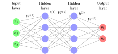
Figure 1. A 4-layer feedforward DNN with two hidden layers.

2.2. Neural Network Robustness Verification

Despite the challenge in verifying the correctness of DNNs, formal verification is still useful to verify their safety-critical properties. One of the most important properties is robustness, stating that the prediction of a neural network is still unchanged even if the input is manipulated under a reasonable range:

Definition 0 (Neural Network Robustness).

A neural network $F:\mathbb{R}^{n}\rightarrow\mathbb{R}^{m}$ is called robust with respect to an input $x_{0}$ and an input region $\Omega$ around $x_{0}$ if $\forall x\in\Omega,\Phi(x)=\Phi(x_{0})$ holds.

Usually, input region $\Omega$ around input $x_{0}$ is defined by a $\ell_{p}$-norm ball around $x_{0}$ with a radius of $\epsilon$, i.e. $\mathbb{B}_{p}(x_{0},\epsilon)=\{x|\|x-x_{0}\|_{p}\leq\epsilon\}$. In this paper, we focus on the infinity norm and verify the robustness of the neural network in $\mathbb{B}_{\infty}(x_{0},\epsilon)$ on image classification tasks. A corresponding robust verification problem is to compute the largest $\epsilon_{0}$ s.t. neural network $F$ is robust in $\mathbb{B}_{\infty}(x_{0},\epsilon_{0})$. The largest $\epsilon$ is called a certified lower bound, which is a metric for measuring both the robustness of neural networks and the precision of robustness verification approaches. Another problem is to compute the ratio of pictures that can be classified correctly when given a fixed $\epsilon$, and that is called a verified robustness ratio.

Assuming that the output label of $x_{0}$ is $c$, i.e. $\Phi(x_{0})=c$, proving $F$’s robustness in Definition 2.1 is equivalent to showing $\forall x\in\Omega,\forall\ell\in L/\{c\},F_{c}(x)-F_{\ell}(x)>0$ holds. Thus, the verification problem is equivalent to solving the following optimization problem:

(1) $$\min_{x\in\Omega}(F_{c}(x)-\max_{\ell\in L/\{c\}}(F_{\ell}(x)))$$

We can conclude that $F$ is robust in $\Omega$ if the result is positive. Otherwise, there exists some input $x^{\prime}$ in $\Omega$ and $\ell^{\prime}$ in $L/\{c\}$ such that $F_{\ell^{\prime}}(x^{\prime})\geq F_{c}(x^{\prime})$. Namely, the probability of classifying $x^{\prime}$ by $F$ to $\ell^{\prime}$ is greater than or equal to the one to $c$, and consequently, $x^{\prime}$ may be classified as $\ell^{\prime}$, meaning that $F$ is not robust in $\Omega$.

2.3. Verification via Linear Over-Approximation

The optimization problem in Equation 1 is computationally expensive, and it is typically impractical to compute the precise solution. The root reason for the high computational complexity of the problem is the non-linearity of the activation function $\sigma$. Even when $\sigma$ is piece-wise linear, e.g., the commonly used ReLU ($\sigma(x)=\max(x,0)$), the problem is NP-complete (Katz et al., 2017). A pragmatic solution to simplify the verification problem is to over-approximate $\sigma(x)$ by linear constraints and symbolic propagation and transform it into an efficiently-solvable linear programming problem (Wang et al., 2018, 2022).

Definition 0 (Linear Over-Approximation).

Let $\sigma(x)$ be a non-linear function on $[l,u]$ and $h_{L}(x)=\alpha_{L}x+\beta_{L},h_{U}(x)=\alpha_{U}x+\beta_{U}$ be two linear functions for some $\alpha_{L},\alpha_{U},\beta_{L},\beta_{U}\in\mathbb{R}$. $h_{L}(x)$ and $h_{U}(x)$ are called the lower and upper linear bounds of $\sigma(x)$ on $[l,u]$ respectively if $h_{L}(x)\leq\sigma(x)\leq h_{U}(x)$ holds for all $x$ in $[l,u]$.

By Definition 2.2, we can simplify Equation 1 to the following efficiently solvable linear optimization problem. Note here that $z$ is an interval, instead of a number:

(2) $$\begin{split}&\min(\min(z_{c}^{(m)}(x))-\max(z_{\ell}^{(m)}(x)))\\ s.t.\quad&z^{(i)}(x)=W^{(i)}\hat{z}^{(i-1)}(x)+b^{(i)},i\in{1,...,m}\\ &h_{L}^{(i)}(x)\leq\hat{z}^{(i)}(x)\leq h_{U}^{(i)}(x),i\in{1,...,m-1}\\ &x\in\Omega,\ell\in L/c,\hat{z}^{(0)}(x)=[x,x]\end{split}$$

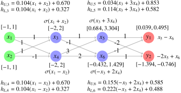
Figure 2. Verifying the robustness of a 4-layer Sigmoid network by the linear over-approximation.

Example 0.

Let us consider the example in Figure 2, which shows the verification process of a simple neural network based on linear approximation. It is a fully-connected neural network with two hidden layers, $x_{1},x_{2}$ are input neurons, and $y_{1},y_{2}$ are output neurons. The intervals represent the range of neurons before the application of the activation function. We conduct linear bounds for each neuron with an activation function using the information of intervals. $h_{U,i}$ and $h_{L,i}$ are the upper and lower linear bounds of $\mathit{\sigma}(x_{i})$ respectively. From the computed intervals of output neuron, we have $\min(y_{1})-\max(y_{2})>0$ for all the possible $(x_{1},x_{2})$ in the input domain $[-1,1]\times[-1,1]$. Consequently, we can conclude that the network is robust in the input domain with respect to the class corresponding to $y_{1}$.

Definition 0 (Approximation Soundness).

Given a neural network $F$ and its input region $\Omega$, a linear over-approximation is called sound if, for all $x$ in $\Omega$, we have $F_{L}(x)\leq F(x)\leq F_{U}(x)$, where $F_{L}$ and $F_{U}$ are the approximated lower and upper bounds of $F$.

The essence of the soundness lies in the actual output range of a network on each output neuron being enclosed by the one after over-approximation. The guarantee of no input in $\Omega$ misclassified by an over-approximated network implies that there must be no input in $\Omega$ misclassified by the original network.

The approximation inevitably introduces the overestimation of output ranges. In Example 2.3, the real output range of $y_{1}$ is $[0.127,0.392]$, which is computed by solving the optimization problems of minimizing and maximizing $y_{1}$, respectively. The one computed by over-approximation is $[0.039,0.495]$. We use the increase rate of an output range with and without the over-approximation to measure the overestimation. Specifically, let $s_{over}$ and $s_{act}$ be the lengths of the overestimated interval and the actual one, respectively. The overestimation ratio $r$ is $\frac{s_{over}-s_{act}}{s_{act}}$, which can be up to 72.08% for $y_{1}$, even for such a simple neural network in Example 2.3.

The overestimation introduced by over-approximation usually renders verifying an actual robust neural network infeasible (also known as incompleteness). For instance, when we have $\min(y_{1})-\max(y_{2})<0$ by solving Problem 2, there may be two reasons. One is that there exists some input such that the output on $y_{1}$ is indeed less than the one on $y_{2}$; the other reason is that the overestimation of $y_{1}$ and $y_{2}$ causes inequality. The network is robust in the latter case while not in the former; however, the algorithms simply report unknown as they cannot distinguish the underlying causes.

2.4. Variant Approximation Tightness Definitions

Reducing the overestimation of approximation is the key to reducing failure cases. The precision of approximation is characterized by the notion of tightness (Zhang et al., 2022b). Many efforts have been made to define the tightest possible approximations. The tightness definitions can be classified into neuron-wise and network-wise categories.

1) Neuron-wise Tightness. The tightness of activation functions’ approximations can be measured independently. Given two upper bounds $h_{U}(x)$ and $h^{\prime}_{U}(x)$ of activation function $\sigma(x)$ on the interval $[l,u]$, $h_{U}(x)$ is apparently tighter than $h^{\prime}_{U}(x)$ if $h_{U}(x)<h^{\prime}_{U}(x)$ for any $x$ in $[l,u]$ (Lyu et al., 2020). However, when $h_{U}(x)$ and $h^{\prime}_{U}(x)$ intersect between $[l,u]$, their tightness becomes non-comparable. Another neuron-wise tightness metric is the area size of the gap between the bound and the activation function, i.e., $\int_{l}^{u}(h_{U}(x)-\sigma(x))dx$. A smaller area implies a tighter approximation (Henriksen and Lomuscio, 2020; Müller et al., 2022b). Apparently, an over-approximation that is tighter than another by the definition of (Lyu et al., 2020) is also tighter by the definition of (Henriksen and Lomuscio, 2020), but not vice versa. What’s more, another metric is the output range of the linear bounds. An approximation is considered to be the tightest if it preserves the same output range as the activation function (Zhang et al., 2022b).

2) Network-wise Tightness. Recent studies have shown that neuron-wise tightness does not always guarantee that the compound of all the approximations of the activation functions in a network is tight too (Zhang et al., 2022b). This finding explains why the so-called tightest approaches based on their neuron-wise tightness metrics achieve the best verification results only for certain networks. It inspires new approximation approaches that consider multiple and even all the activation functions in a network to approximate simultaneously. The compound of all the activation functions’ approximations is called the network-wise tightest with respect to an output neuron if the neuron’s output range is the precisest.

Unfortunately, finding the network-wise tightest approximation has been proved a non-convex optimization problem, and thus computationally expensive (Lyu et al., 2020; Zhang et al., 2022b). From a pragmatic viewpoint, a neuron-wise tight approximation is useful if all the neurons’ composition is also network-wise tight. The work (Zhang et al., 2022b) shows that there exists such a neuron-wise tight approach under certain constraints when the networks are monotonic. However, their approach does not guarantee to be optimal when the neural networks contain both positive and negative weights.

Note that an activation function can be approximated more tightly using two more pieces of linear bounds. In this paper, we focus on one-piece linear approximation defined in Definition 2.2. This method is the most efficient since the reduced problem is a linear programming problem that can be efficiently solved in polynomial time. For piece-wise approximations, it is challenging because as the number of linear bounds drastically blows up, and the corresponding reduced problem is proved to be NP-complete (Singh et al., 2019).

3. Motivation

In this section we show that the over-approximation inevitably introduces overestimation. We observe that the overestimation of intervals is accumulatively propagated as the intervals are propagated on a layer basis. We then identify an important factor called approximation domain for explaining why existing, so-called tightest over-approximation approaches still introduce large overestimation. Finally, we illustrate that the precise approximation domain and the tight over-approximation are interdependent.

3.1. Interval Overestimation Propagation

Neural network verification methods based on over-approximation will inevitably introduce overestimation more or less, as shown in Section 2.3. For the approximation of an activation function, if the maximum value of its upper bound is larger than the maximum value of the actual value, or the minimum value of its lower bound is smaller than the minimum value of the actual value, the approximation is imprecise and introduces too much overestimation.

In our experiment, we found that the overestimation can be accumulated and propagated layer by layer. We evaluate four state-of-the-art linear over-approximation approaches, including NeWise (NW) (Zhang et al., 2022b), DeepCert (DC) (Wu and Zhang, 2021), VeriNet (VN) (Henriksen and Lomuscio, 2020), and RobustVerifier (RV) (Lin et al., 2019), to verify the neural network model defined in Figure 2 with $50,000$ different weights and input intervals, and record the size of real intervals and overestimated intervals during the process. Figure 3 shows the overestimation of each neuron with the network in Figure 2, together with the overestimation distribution of the $50,000$ cases for $y_{1}$ and $y_{2}$. In Figure 3(a), the overestimation is over $400\%$ for $x_{3}$, $x_{4}$, $x_{5}$, $x_{6}$, and around $50\%$ for $y_{1}$, $y_{2}$. Note that the overestimation of $y_{1}$ and $y_{2}$ is smaller than the ones in the hidden layers. This is due to the non-monotonicity of neural networks and the normalization of activation functions. We can find in Figure 3(b) that most of the overestimations are distributed between $50\%$ and $100\%$, while it is over $300\%$ in more than $10\%$ cases.

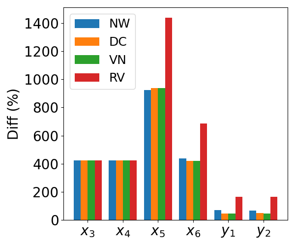
(a) Overestimation on a network.

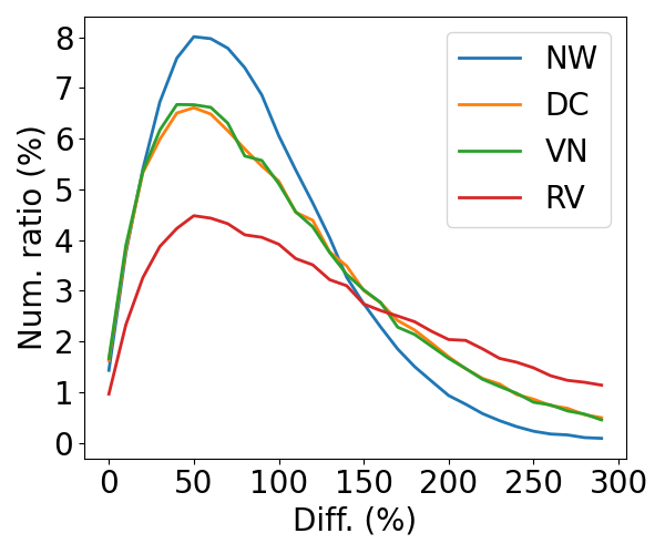
(b) Overestimation distribution.

Figure 3. The overestimation of each neuron in the network in Figure 2 (a) and the overestimation distribution on 50,000 variant networks with the same network architecture (b).

There are two main reasons for the accumulative propagation. One apparent reason is the over-approximations of activation functions, which is inevitable but can be reduced by defining tight ones. The other reason is that over-approximations must be defined on overestimated domains of the activation function to guarantee the soundness of it. This further introduces overestimation to approximations as the domains’ overestimation increases. Due to the layer dependency in neural networks, such dual overestimation is accumulated and propagated to the output layer.

3.2. Approximation Domain

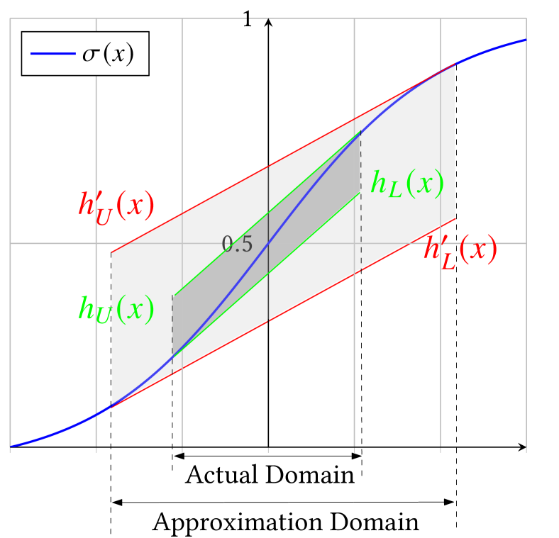
(a) Tangent line at end points (Zhang et al., 2022b).

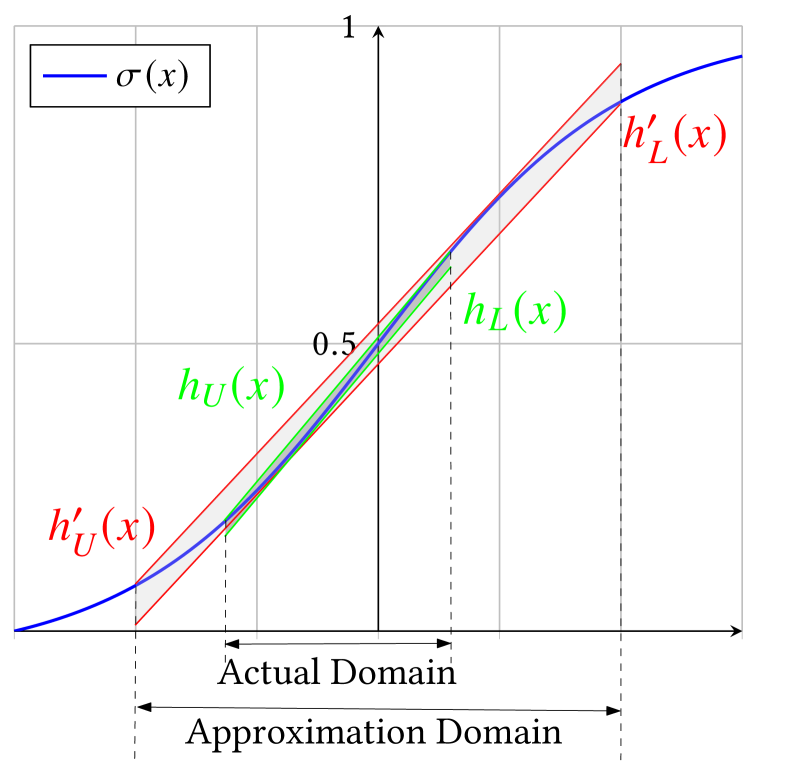
(b) Minimal area (Henriksen and Lomuscio, 2020).

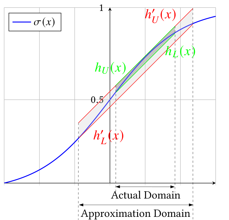
(c) Parallel line (Wu and Zhang, 2021; Zhang et al., 2018).

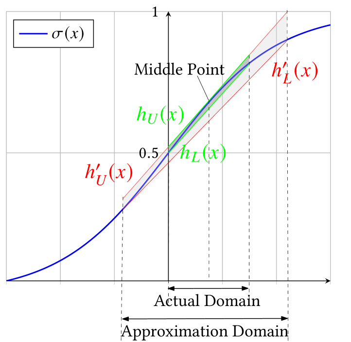
(d) Tangent line at middle point (Henriksen and Lomuscio, 2020).

Figure 4. The differences between the linear over-approximations that are defined on the estimated approximation and the actual one respectively according to the four state-of-the-art approaches. The red lines refer to the upper and lower bounds defined on approximation domains, and the green lines refer to those defined on actual domains. The light and dark gray areas represent the corresponding overestimation introduced by the over-approximations, respectively.

To justify the second reason for the accumulative propagation in Section 3.1, we introduce the notion of approximation domain, to represent the domain of activation functions, on which over-approximations are defined.

Definition 0 (Approximation Domain).

Given a neural network $F$ and an input region $\mathbb{B}_{\infty}(x_{0},\epsilon)$, the approximation domain of the $r$-th hidden neuron in the $i$-th layer is $[l_{r}^{(i)},u_{r}^{(i)}]$, where,

$$\begin{split}l_{r}^{(i)}=&\min z_{r}^{(i)}(x),u_{r}^{(i)}=\max z_{r}^{(i)}(x)\\ s.t.\quad&z^{(j)}(x)=W^{(j)}\hat{z}^{j-1}(x)+b^{(j)},j\in{1,...,i}\\ &h_{L}(z^{(j)}(x))\leq\hat{z}^{(j)}(x)\leq h_{U}(z^{(j)}(x)),j\in{1,...,i-1}\\ &x\in\mathbb{B}_{\infty}(x_{0},\epsilon),\hat{z}^{(0)}(x)=x\end{split}$$

Definition 3.1 formulates the way of the existing over-approximation approaches (Zhang et al., 2022b; Henriksen and Lomuscio, 2020; Zhang et al., 2018; Wu and Zhang, 2021) to compute overestimated domains of activation functions for defining their over-approximations. Given two different approximation domains $[l_{r},u_{r}]$ and $[l^{\prime}_{r},u^{\prime}_{r}]$, we say $[l_{r},u_{r}]$ is more precise than $[l^{\prime}_{r},u^{\prime}_{r}]$ if $l_{r}\geq l^{\prime}_{r}$ and $u_{r}\leq u^{\prime}_{r}$. Let us consider the activation functions on neurons $x_{5}$ and $x_{6}$ in Figure 2 as an example. Their domains are estimated based on the approximations of $x_{3}$ and $x_{4}$ by solving the corresponding linear programming problems in Definition 3.1. The approximation domains are $[0.684,3.304]$ and $[-0.432,1.429]$, respectively. As shown in Figure 3(a), they are much overestimated compared with the actual ones.

3.3. The Overestimation Interdependency

We show the interdependency between the two problems of defining tight over-approximations for activation functions and computing the precise approximation domains. The interdependency means that tighter over-approximations of activation functions result in more precise approximation domains and vice versa. Here we follow the approximation tightness definition in (Lyu et al., 2020), by which a lower bound $h_{L}(x)$ is called tighter than another $h^{\prime}_{L}(x)$ if $h_{L}(x)\geq h^{\prime}_{L}(x)$ holds for all $x$ in the approximation domain of $\sigma$. Likewise, an upper bound $h_{U}(x)$ is tighter than another $h^{\prime}_{U}(x)$ if $h_{U}(x)\leq h^{\prime}_{U}(x)$. Apparently, a tighter approximation by definition (Lyu et al., 2020) is still tighter by the minimal-area-based definition (Henriksen and Lomuscio, 2020).

Theorem 3.2.

Suppose that there are two over-approximations $h_{L}(z^{(j)}(x)),h_{U}(z^{(j)}(x))$ and ${h^{\prime}}_{L}(z^{(j)}(x)),{h^{\prime}}_{U}(z^{(j)}(x))$ for each $z^{(j)}(x)$ in Definition 3.1 and $h_{L}(z^{(j)}(x)),h_{U}(z^{(j)}(x))$ are tighter than ${h^{\prime}}_{L}(z^{(j)}(x)),{h^{\prime}}_{U}(z^{(j)}(x))$, respectively. The approximation domain $[l_{r}^{(i)},u_{r}^{(i)}]$ computed by $h_{L}(z^{(j)}(x)),h_{U}(z^{(j)}(x))$ must be more precise than the one $[{l^{\prime}}_{r}^{(i)},{u^{\prime}}_{r}^{(i)}]$ by ${h^{\prime}}_{L}(z^{(j)}(x)),{h^{\prime}}_{U}(z^{(j)}(x))$.

Intuitively, Theorem 3.2 claims that tighter approximations lead to more precise approximation domains for the activation functions of the neurons in subsequent layers of a DNN.

Theorem 3.3.

Given two approximation domains $[l_{r}^{(i)},u_{r}^{(i)}]$ and $[{l^{\prime}}_{r}^{(i)},{u^{\prime}}_{r}^{(i)}]$ such that ${l^{\prime}}_{r}^{(i)}<l_{r}^{(i)}$ and $u_{r}^{(i)}<{u^{\prime}}_{r}^{(i)}]$, for any over-approximation $({h^{\prime}}_{L}(z^{(j)}(x)),{h^{\prime}}_{U}(z^{(j)}(x)))$ of continuous function $\sigma(x)$ on $[{l^{\prime}}_{r}^{(i)},{u^{\prime}}_{r}^{(i)}]$, there exists an over-approximation $(h_{L}(z^{(j)}(x))$, $h_{U}(z^{(j)}(x)))$ on $[l_{r}^{(i)},u_{r}^{(i)}]$ such that $\forall z^{(j)}(x)\in[l_{r}^{(i)},u_{r}^{(i)}],h^{\prime}_{L}(x)\leq h_{L}(z^{(j)}(x)),h^{\prime}_{U}(x)\geq h_{U}(z^{(j)}(x))$.

Theorem 3.3 claims that more precise approximation domains lead to tighter over-approximations of the activation function. Altogether, the two theorems preserve the tightness of an approximation through propagation in a neural network. The proofs of Theorems 3.2 and 3.3 are given in Appendix A.

The above two theorems show the overestimation interdependency of the two problems. As examples, Figure 4 depicts the differences between the over-approximations that are defined on overestimated approximation domains and the actual domains based on the corresponding approximation approaches (Zhang et al., 2022b; Henriksen and Lomuscio, 2020; Wu and Zhang, 2021; Zhang et al., 2018). Apparently, there exist much tighter over-approximations if we can reduce the overestimation of approximation domains. These examples show the importance of more precise approximation domains for activation functions to define tighter over-approximations.

It is worth mentioning that it is almost impractical to define over-approximations directly on the actual domain of activation functions for non-trivial neural networks, e.g., those which have two or more hidden layers. The reason is that computing the actual domains is at least as computationally expensive as the neural network verification problem per se. If we could compute the domains for all the activation functions on hidden neurons, the robustness verification problem would then be efficiently solvable by solving the linear constraints between the last hidden layer and the output layer by using linear programming.

4. The Dual-Approximation Approach

In this section we present our dual-approximation approach for defining tight over-approximation for activation functions guided by under-approximations. Specifically, we propose two algorithms to compute underestimated approximation domains for each activation function and define different over-approximation strategies according to both overestimated and underestimated domains.

4.1. Approach Overview

Figure 5 depicts an illustration of our dual-approximation approach and the comparisons with those approaches defined only based on approximation domains. For each activation function, we compute an overestimated and an underestimated approximation domain, denoted by $[l_{\mathit{\mathit{over}}},u_{\mathit{over}}]$ and $[l_{\mathit{under}},u_{\mathit{under}}]$, respectively. Underestimated domains provide useful information for defining over-approximations. Let $h(x)$ be a linear lower or upper bound of $\sigma$ on the interval $[l_{\mathit{under}},u_{\mathit{under}}]$. We take it as a linear over-approximation lower or upper bound for $\sigma$ on the approximation domain $[l_{\mathit{\mathit{over}}},u_{\mathit{over}}]$ if it satisfies the condition in Definition 2.2. According to Theorem 3.3, we can define a tighter $h(x)$ on $[l_{\mathit{under}},u_{\mathit{under}}]$ than those defined on $[l_{\mathit{over}},u_{\mathit{over}}]$ and make sure $h(x)$ is a valid over-approximation bound on $[l_{\mathit{\mathit{over}}},u_{\mathit{over}}]$. Thus, the underestimated domain is used to guarantee the over-approximation’s tightness, while the approximation domain to guarantee its soundness. We therefore call it a dual-approximation approach.

Figure 5. An illustration of our dual-approximation approach and comparison with other over-approximation approaches.

As shown in Figure 5, we take the tangent line at $(l_{\mathit{under}},\sigma(l_{\mathit{under}}))$ as the lower bound of $\sigma$. Apparently, this lower bound is much tighter than the one defined by the tangent line at $(l_{\mathit{over}},\sigma(l_{\mathit{over}}))$ (the dark green line according to the approach by NeWise (Zhang et al., 2022b)) on the actual domain $[l_{\mathit{actual}},u_{\mathit{actual}}]$ of $\sigma$. It is also tighter than the green tangent line parallel to the upper bound, according to the approaches in DeepCert (Wu and Zhang, 2021) and RobustVerifier (Lin et al., 2019).

4.2. Under-Approximation Algorithms

We introduce two approaches, i.e., Monte Carlo and gradient-based, for underestimating the actual domain of the activation functions. In other word, we propose two strategies to compute $[l_{\mathit{under}},u_{\mathit{under}}]$. The two strategies are complementary in that the former is more efficient but computes less precise underestimated input domain, while the latter performs in the opposite way.

Input : $F$: a network; $x_{0}$: an input to $F$; $\epsilon$: a $\ell_{\infty}$-norm radius; $n$: number of samples

Output : $l_{L,r}^{(i)},u_{L,r}^{(i)}$ for each hidden neuron $r$ on layer $i$

1 Randomly generate $n$ samples $S_{n}$ from $\mathbb{B}_{\infty}(x_{0},\epsilon)$;

$l_{L}\leftarrow\infty,u_{L}\leftarrow-\infty$;

  // Initialize all upper and lower bounds

2 for each sample $x_{p}$ in $S_{n}$ do

3       for each hidden layer $i$ do

4             for each neuron $r$ on layer $i$ do

                   $v_{p,r}^{(i)}:=F_{r}^{(i)}(x_{p})$;

                    // Compute the output of neuron $r$

                   $l_{L,r}^{(i)}\leftarrow\min(l_{L,r}^{(i)},v_{p,r}^{(i)})$ ;

                    // Update $r$’s lower bound

                   $u_{L,r}^{(i)}\leftarrow\max(u_{L,r}^{(i)},v_{p,r}^{(i)})$;

                    // Update $r$’s upper bound

5                  

6            

7      

Algorithm 1 The Monte Carlo Approach.

The Monte Carlo Approach. A simple yet efficient approach for under-approximation is to randomly generate a number of valid samples and feed them into the network to track the reachable bounds of each hidden neuron’s input. A sample is valid if the distance between it and the original input is less than a preset perturbation distance $\epsilon$.

Algorithm 1 shows the pseudo-code of the Monte Carlo approach. First, we randomly generate $n$ valid samples from $\mathbb{B}_{\infty}(x_{0},\epsilon)$ (Line 1) and initialize the lower and upper bounds $l_{L,r}^{(i)}$ and $u_{L,r}^{(i)}$ of each hidden neuron (Line 2). Then we feed each sample into the network (Line 3), record the input value $v^{(i)}_{p,r}$ of each activation function (Line 6), and update the corresponding lower or upper bound by $v^{(i)}_{L,r}$ (Lines 7-8). The time complexity of Algorithm 1 is $O(n\sum_{i=1}^{m}k_{i}k_{i-1})$, where $m$ refers to the layer of the neural network, and $k_{i}$ refers to the number of neurons of layer $i$.

The Gradient-Based Approach. The conductivity of neural networks allows us to approximate the actual domain of each hidden neuron by gradient descent (Ruder, 2016). The basic idea of gradient descent is to compute two valid samples according to the gradient of an objective function to minimize and maximize the output value of the function, respectively. Using gradient descent, we can compute locally optimal lower and upper bounds as the underestimated input domains of activation functions.

Algorithm 2 shows the pseudo-code of the gradient-based approach. Its inputs include a neural network $F$, an input $x_{0}$ of $F$, an $\ell_{\infty}$-norm radius $\epsilon$, and a step length $a$ of gradient descent. It returns an underestimated input domain for each neuron on the hidden layers. It gets function $F^{(i)}_{r}$ of the neural network on neuron $r$ (Line 3), computes its gradient, and records its sign $\eta^{i}_{r}$ as the direction to update $x_{0}$ (Line 4). Then, the gradient descent is conducted one step forward to generate a new input $x_{\mathit{lower}}$ (Line 5). $x_{\mathit{lower}}$ is then modified to make sure it is in the normal ball. By feeding $x_{\mathit{lower}}$ to $F^{(i)}_{r}$, we obtain an under-approximated lower bound $l_{L,r}^{(i)}$ (Line 7). The upper bound can be computed likewise (Lines 8-10).

Considering the time complexity of Algorithm 2, we need to compute the gradient for each neuron on the $i$th hidden layer, of which time complexity is $O(\sum_{j=1}^{i}k_{j}k_{j-1})$. Thus, given an $m$-hidden-layer network, the time complexity of the gradient-based algorithm is $O(\sum_{i=1}^{m}k_{i}(\sum_{j=1}^{i}k_{j}k_{j-1}))$. This is higher than the time complexity of the Monte Carlo algorithm, while it obtains a more precise underestimated domain. We compare the efficiency and effectiveness of the two algorithms in Experiment II.

Input : $F$: a network; $x_{0}$: an input to $F$; $\epsilon$: a $\ell_{\infty}$-norm radius; $a$: the step length of gradient descent

Output : $l_{L,r}^{(i)},u_{L,r}^{(i)}$ for each neuron $r$ in each hidden layer $i$

1 for each hidden layer $i={1,\ldots,m}$ do

2       for each neuron $r$ on layer $i$ do

3             Get the function $F_{r}^{(i)}$of neuron $r$;

             $\eta_{r}^{(i)}\leftarrow sign(F_{r}^{(i)^{\prime}}(x_{0}))$;

              // Get the sign of gradient of $r$

             $x_{\mathit{lower}}\leftarrow x_{0}-a\eta_{r}^{(i)}$;

              // One-step forward

             Cut $x_{\mathit{lower}}$ s.t. $x_{\mathit{lower}}\in\mathbb{B}_{\infty}(x_{0},\epsilon)$;

              // Make $x_{\mathit{lower}}$ valid

             $l_{L,r}^{(i)}\leftarrow F_{r}^{(i)}(x_{\mathit{lower}})$;

              // Compute and store the lower bound

             $x_{\mathit{upper}}\leftarrow x_{0}+a\eta_{r}^{(i)}$;

              // Compute the upper case

4             Cut $x_{\mathit{upper}}$ s.t. $x_{\mathit{upper}}\in\mathbb{B}_{\infty}(x_{0},\epsilon)$

             $u_{L,r}^{(i)}\leftarrow F_{r}^{(i)}(x_{\mathit{upper}})$ ;

              // Compute and store the upper bound

5            

6      

Algorithm 2 The Gradient-Based Approach.

4.3. Over-Approximation Strategies

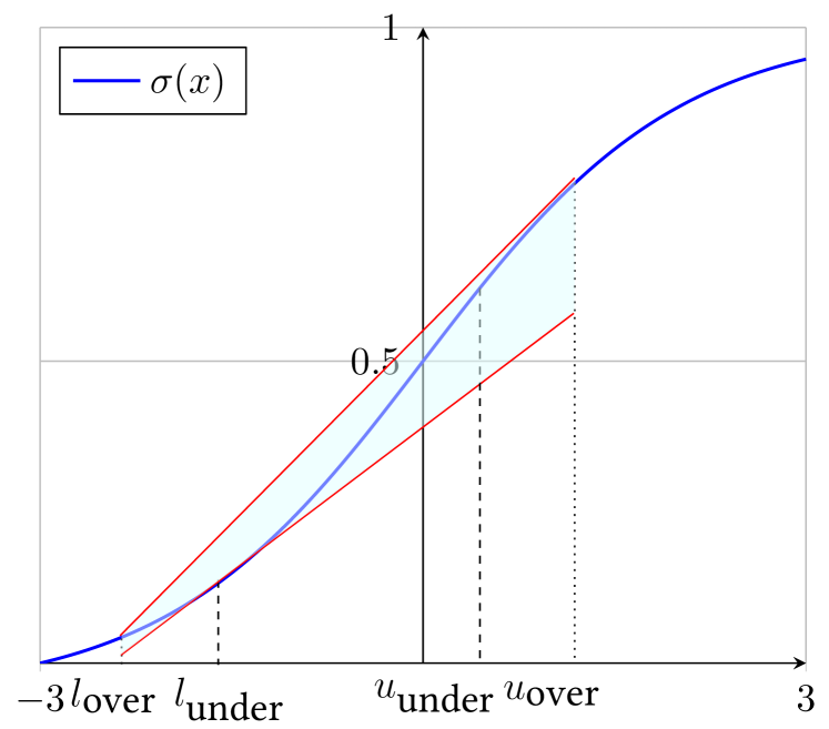
(a) I: $\sigma^{\prime}(l_{\mathit{over}})<k<\sigma^{\prime}(u_{\mathit{over}})$.

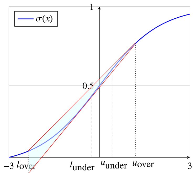
(b) I: $\sigma^{\prime}(l_{\mathit{over}})<k<\sigma^{\prime}(u_{\mathit{over}})$

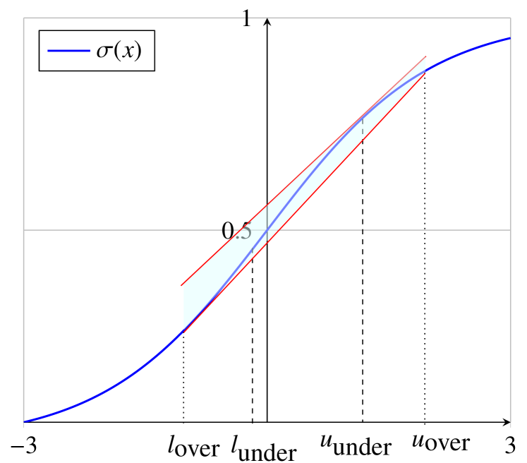
(c) II: $\sigma^{\prime}(l_{\mathit{over}})>k>\sigma^{\prime}(u_{\mathit{over}})$.

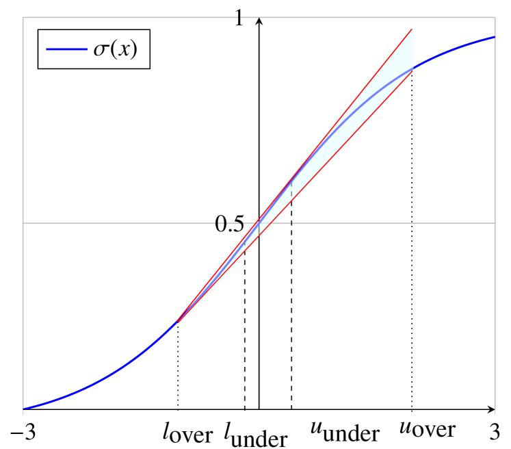
(d) II: $\sigma^{\prime}(l_{\mathit{over}})>k>\sigma^{\prime}(u_{\mathit{over}})$.

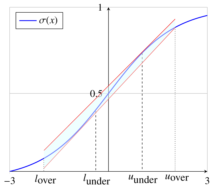
(e) III: $\sigma^{\prime}(l_{\mathit{over}})\!<\!k\wedge\sigma^{\prime}(u_{\mathit{over}})\!<\!k$.

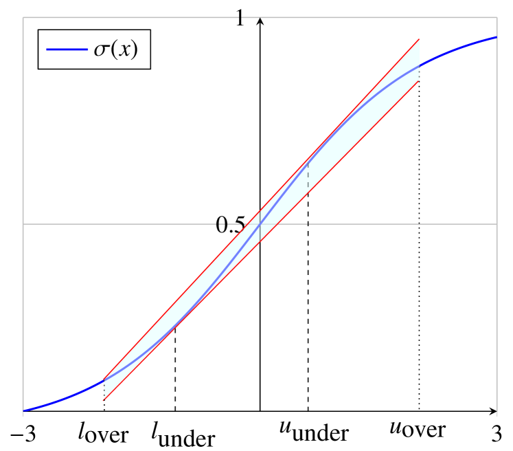
(f) III: $\sigma^{\prime}(l_{\mathit{over}})\!<\!k\wedge\sigma^{\prime}(u_{\mathit{over}})\!<\!k$.

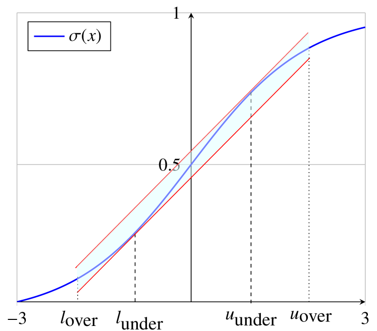
(g) III: $\sigma^{\prime}(l_{\mathit{over}})\!<\!k\!\wedge\!\sigma^{\prime}(u_{\mathit{over}})\!<\!k$.

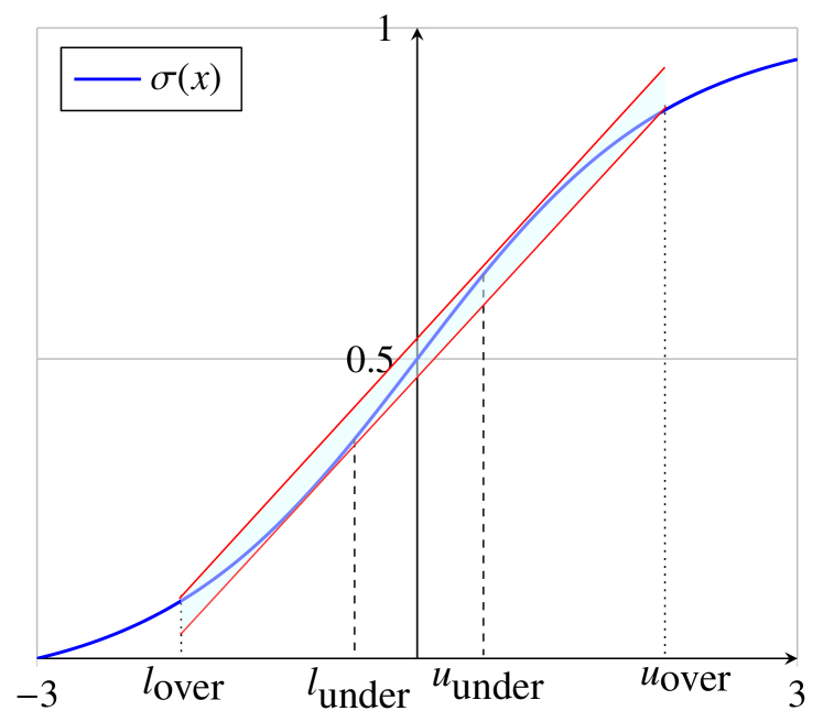
(h) III: $\sigma^{\prime}(l_{\mathit{over}})\!<\!k\!\wedge\!\sigma^{\prime}(u_{\mathit{over}})\!<\!k$.

Figure 6. The linear over-approximation based on overestimated and underestimated approximation domains.

We omit the superscript and subscript and consider finding the approximation method of $\sigma(x)$ with the information of upper and lower approximation domains. We assume that the lower approximation domain of input $x$ is $[l_{\mathit{under}},u_{\mathit{under}}]$ and the upper approximation interval is $[l_{\mathit{over}},u_{\mathit{over}}]$. As in (Wu and Zhang, 2021), we consider three cases according to the relation between the slopes of $\sigma$ at the two endpoints of upper approximation interval $\sigma^{\prime}(l_{\mathit{over}})$, $\sigma^{\prime}(u_{\mathit{over}})$ and $k=\frac{\sigma(u_{\mathit{over}})-\sigma(l_{\mathit{over}})}{u_{\mathit{over}}-l_{\mathit{over}}}$.

Case I. When $\sigma^{\prime}(l_{\mathit{over}})<k<\sigma^{\prime}(u_{\mathit{over}})$, the line connecting the two endpoints is the upper bound. For the lower bound, the tangent line of $\sigma$ at $l_{\mathit{under}}$ is chosen if it is sound (Figure 6(a)), otherwise the tangent line of $\sigma$ at $d$ crossing $(u_{\mathit{over}},\sigma(u_{\mathit{over}}))$ is chosen (Figure 6(b)). Namely, we have $h_{U}(x)=k(x-u_{over})+\sigma(u_{over})+$, and

(3) $$h_{L}(x)=\begin{cases}\sigma^{\prime}(l_{\mathit{under}})(x-l_{\mathit{under}})+\sigma(l_{\mathit{under}}),&l_{\mathit{under}}<d\\ \sigma^{\prime}(d)(x-d)+\sigma(d),&l_{\mathit{under}}\geq d.\end{cases}$$

Case II. When $\sigma^{\prime}(l_{\mathit{over}})>k>\sigma^{\prime}(u_{\mathit{over}})$, it is the symmetry of Case 1. the line connecting the two endpoints can be the lower bound. For upper bound, the tangent line of $\sigma$ at $u_{\mathit{under}}$ is chosen if it is sound (Figure 6(c)), otherwise the tangent line of $\sigma$ at $d$ crossing $(l_{\mathit{under}},\sigma(l_{\mathit{under}}))$ is chosen (Figure 6(d)). That is, $h_{L}(x)=k(x-l_{over})+\sigma(l_{over})$, and

(4) $$h_{U}(x)=\begin{cases}\sigma^{\prime}(u_{\mathit{under}})(x-u_{\mathit{under}})+\sigma(u_{\mathit{under}}),&u_{\mathit{under}}>d\\ \sigma^{\prime}(d)(x-d)+\sigma(d),&u_{\mathit{under}}\leq d.\end{cases}$$

Case III. When $\sigma^{\prime}(l_{\mathit{over}})<k$ and $\sigma^{\prime}(u_{\mathit{over}})<k$, we first consider the upper bound. If the tangent line of $\sigma$ at $u_{\mathit{under}}$ is sound, we choose it to be the upper bound (Figure 6(e) and Fig 6(g)); otherwise we choose the tangent line of $\sigma$ at $d_{1}$ crossing $(l_{\mathit{under}},\sigma(l_{\mathit{under}}))$ (Figure 6(f) and Figure 6(h)). Then we consider the lower bound. The tangent line of $\sigma$ at $l_{\mathit{under}}$ is chosen if it is sound (Figure 6(f) and Figure 6(g)), otherwise we choose the tangent line of $\sigma$ at $d_{2}$ crossing $(u_{\mathit{over}},\sigma(u_{\mathit{over}}))$ (Figure 6(e) and Figure 6(h)). Namely, we have:

(5) $$h_{U}(x)=\begin{cases}\sigma^{\prime}(u_{\mathit{\mathit{under}}})(x-u_{\mathit{under}})+\sigma(u_{\mathit{under}}),&u_{\mathit{under}}>d_{1}\\ \sigma^{\prime}(d_{1})(x-d_{1})+\sigma(d_{1}),&u_{\mathit{under}}\leq d_{1},\end{cases}$$

(6) $$h_{L}(x)=\begin{cases}\sigma^{\prime}(l_{\mathit{under}})(x-l_{\mathit{under}})+\sigma(l_{\mathit{under}}),&l_{\mathit{under}}<d_{2}\\ \sigma^{\prime}(d_{2})(x-d_{2})+\sigma(d_{2}),&l_{\mathit{under}}\geq d_{2}.\end{cases}$$

The goal of our approximation strategy is to make the overestimated output interval as close as possible to the actual one of each hidden neuron. An over-approximation is the provably tightest neuron-wise if it preserves the same output interval as the activation function on the actual domain (Zhang et al., 2022b). As described in Theorem 3.3, a more precise range allows us to define a tighter over-approximation. Under the premise of guaranteeing soundness, we use the guiding significance of the underestimated domain to make the over-approximation closer to the actual domain so as to obtain more precise approximation bounds. Through layer-by-layer transmission, we obtain more accurate intervals for the deeper hidden neurons (by Theorem 3.2), on which tighter over-approximations can be defined (by Theorem 3.3). In this way, the overestimation interdependency during defining over-approximations is alleviated by computing the underestimated domains. The soundness proof for our approach is given in Appendix B.

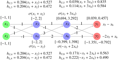
Figure 7. The approximations defined in our approach and the propagated intervals for the network in Figure 2.

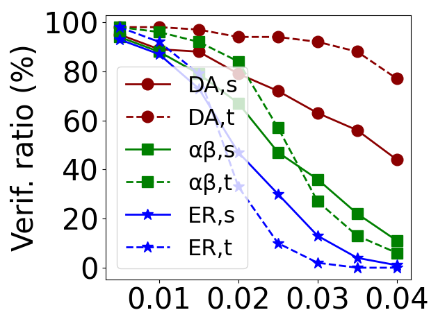
(a) FC 6*500

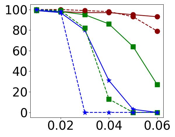
(b) FC PGD 0.1

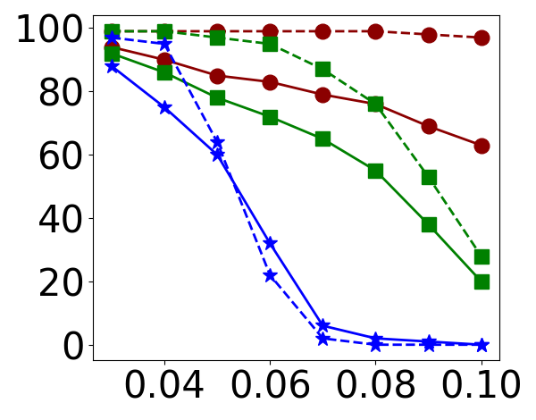
(c) FC PGD 0.3

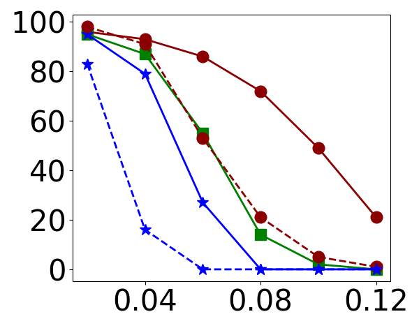
(d) ConvMed

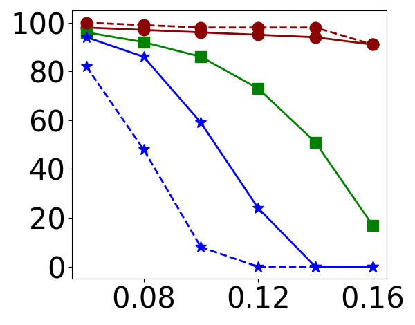
(e) Conv PGD 0.1

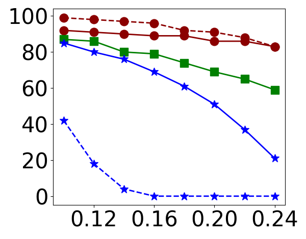
(f) Conv PGD 0.3

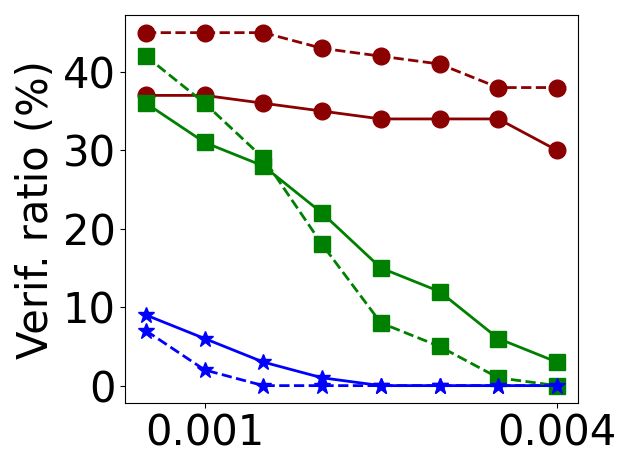
(g) FC 6*500

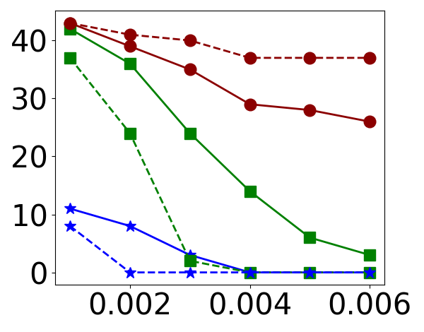
(h) FC PGD 0.0078

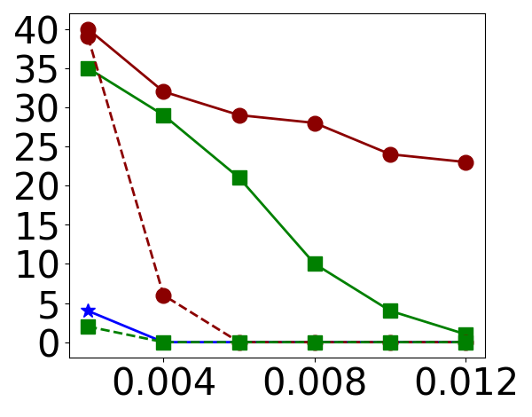
(i) FC PGD 0.0313

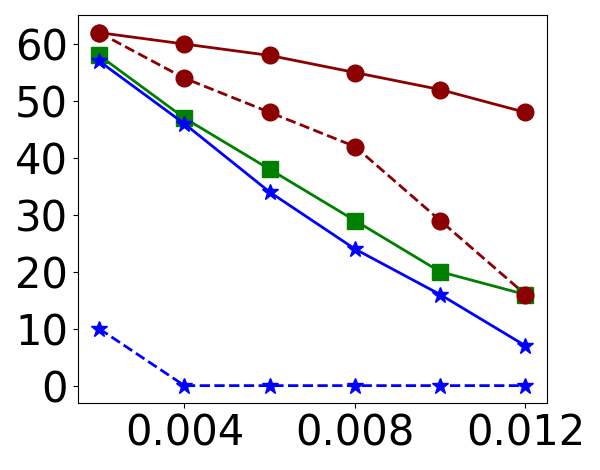
(j) ConvMed

(k) Conv PGD 0.0078

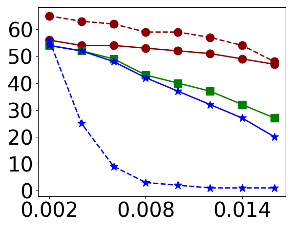
(l) Conv PGD 0.0078

Figure 8. Comparison of the verified robustness rate of DualApp, $\alpha$-$\beta$-CROWN, and ERAN on 24 neural networks and two datasets. (a-f) refer to the comparison on MNIST while (g-l) to CIFAR-10. The horizontal axis represents the perturbation $\epsilon$, and the vertical axis represents the ratio of images that are verified robustness. Legend $DA,s$ refers to the result of DualApp on the neural network with sigmoid activation function, and $ER,t$ refers to the result of ERAN with tanh.

Example 0.

We reconsider the network in Figure 2. Figure 7 shows the approximations and the propagated intervals for neurons in hidden layers and the output layer. As $x_{3},x_{4}$ have precise input intervals, only the activation functions of $x_{5},x_{6}$ need to be under-approximated. Thus, we only need to redefine their approximations according to our approach. We underestimate the input domains of $x_{5},x_{6}$ and use them to guide the over-approximations in our approach. We achieve $9.74\%$ and $0.27\%$ reductions for the overestimation of $y_{1},y_{2}$’s output ranges.

Example 4.1 demonstrates the effectiveness of our proposed dual-approximation approach even when it is applied to only one hidden layer. That is, the overestimation of propagated intervals can be further reduced through defining tighter over-approximations based on both underestimated and approximation domains. Tighter over-approximations can produce more precise verification results, and we will show this experimentally in the next section.

5. Implementation and Evaluation

We implement our dual-approximation approach into a tool called DualApp. We assess it, along with six state-of-the-art tools, with respect to the DNNs with the S-curved activation functions. Our goal is threefold:

1. to demonstrate that, compared to the state of the art, DualApp is more tight on robustness verification results;

2. to explore the hyper-parameter space for our two methods that leverage under-approximation; and

3. to measure the trade-off between these two complementary under-approximation methods.

5.1. Benchmark and Implementation

Competitors. We consider six state-of-the-art DNN robustness verification tools: $\alpha$-$\beta$-CROWN (Zhang et al., 2022a), ERAN (Müller et al., 2022b), NeWise (Zhang et al., 2022b), DeepCert (Wu and Zhang, 2021), VeriNet (Henriksen and Lomuscio, 2020), and RobustVerifier (Lin et al., 2019). They rely on the over-approximation domain to define and optimize linear lower and upper bounds except that ERAN is based on the abstract domain combining floating point polyhedra with intervals (Singh et al., 2019).

Datasets and Neural Networks. In the comparison experiment with $\alpha$-$\beta$-CROWN and ERAN, we collect 24 models exposed by ERAN for MNIST (LeCun et al., 1998) and CIFAR-10 (Krizhevsky et al., 2009), including CNNs and FNNs trained with normal training method and adversarial training method with PGD attack (Wang et al., 2021). These models contain Sigmoid and Tanh activation functions. For NeWise, DeepCert, VeriNet, and RobustVerifier, we collect and train totally 84 convolutional neural networks (CNNs) and fully-connected neural networks (FNNs) on image datasets MNIST, Fashion MNIST (Xiao et al., 2017) and CIFAR-10. Sigmoid, Tanh, and Arctan are contained in these models, respectively. As most researches are based on the ReLU activation function, there are few public neural networks in benchmarks with S-curved activate functions, and their sizes are small.

Metrics. We use two metrics in our comparisons: (i) verified robustness ratio, which is the percentage of images that must be correctly classified under a fixed perturbation $\epsilon$, and (ii) certified lower bound, which is the largest perturbation $\epsilon$ within which all input images must be correctly classified. We consider strong baselines in that we assess DualApp on the benchmarks and metrics for which the competitors report the optimal performance. In particular, we use (i) for the comparison with $\alpha$-$\beta$-CROWN and ERAN as both report the highest verified robustness rate as in, e.g., the 2022 VNN-COMP competition (Müller et al., 2022a).

Implementation. For a fair comparison, we implemented the approximation strategies of NeWise, DeepCert, VeriNet, RobustVerifier, and our dual-approximation algorithm in DualApp using python with the TensorFlow framework. We apply the method used in NeWise to train neural networks and load datasets. We implement the algorithms and strategies defined in Section 4 to compute under-approximation domains and linear upper and lower bounds, thus obtaining the final output intervals and verification results for each image. To compute the certified lower bound, we set the initial value of $\epsilon$ to $0.05$ and update it $15$ times using the dichotomy method based on the verification results.

Experimental Setup. We conducted all the experiments on a workstation equipped with a 32-core AMD Ryzen Threadripper PRO 5975WX CPU, 256GB RAM, and an Nvidia RTX 3090Ti GPU running Ubuntu 22.04.

5.2. Experimental Results

Table 1. Comparison of the verification time among DualApp, $\alpha$-$\beta$-CROWN, and ERAN on 24 neural networks and two datasets. We report the average time of verifying 100 images on 6 neural networks with the same architecture used in Figure 8, e.g., the time of FC models on MNIST refers to the experiments in Figure 8(a)-8(c).

Dataset	Model	DualApp	$\alpha$-$\beta$-CROWN	ERAN
MNIST	FC	3.81s	2.30s	14.39s
	CONV	1.09s	2.25s	3.30s
CIFAR-10	FC	3.12s	4.46s	34.16s
	CONV	1.81s	0.88s	6.46s

Table 2. Comparing the DualApp (DA) and four state-of-the-art tools including NeWise (NW), DeepCert (DC), VeriNet (VN), and RobustVerifier (RV) on the CNNs and FNNs with the Sigmoid activation function. ${\rm CNN}_{l-k}$ denotes a CNN with $l$ layers and $k$ filters of size $3\times 3$ on each layer. ${\rm FNN}_{l\times k}$ denotes a FNN with $l$ layers and $k$ neurons on each layer.

Dataset	Model	Nodes	DA	NW		DC		VN		RV		DA Time (s)	Others Time (s)
			Bounds	Bounds	Impr. (%)	Bounds	Impr. (%)	Bounds	Impr. (%)	Bounds	Impr. (%)
Mnist	${\rm CNN}_{4-5}$	8,690	0.05819	0.05698	2.12	0.05394	7.88	0.05425	7.26	0.05220	11.48	14.70	0.98 $\pm$ 0.02
	${\rm CNN}_{5-5}$	10,690	0.05985	0.05813	2.96	0.05481	9.20	0.05503	8.76	0.05125	16.78	20.13	2.67 $\pm$ 0.29
	${\rm CNN}_{6-5}$	12,300	0.06450	0.06235	3.45	0.05898	9.36	0.05882	9.66	0.05409	19.25	25.09	4.86 $\pm$ 0.34
	${\rm CNN}_{8-5}$	14,570	0.11412	0.09559	19.38	0.08782	29.95	0.08819	29.40	0.06853	66.53	34.39	11.89 $\pm$ 0.21
	${\rm FNN}_{5\times 100}$	510	0.00633	0.00575	10.09	0.00607	4.28	0.00616	2.76	0.00519	21.97	7.10	0.79 $\pm$ 0.05
	${\rm FNN}_{6\times 200}$	1,210	0.02969	0.02909	2.06	0.02511	18.24	0.02829	4.95	0.01811	63.94	8.64	2.82 $\pm$ 0.34
Fashion Mnist	${\rm CNN}_{4-5}$	8,690	0.07703	0.07473	3.08	0.07204	6.93	0.07200	6.99	0.06663	15.61	15.26	1.06 $\pm$ 0.09
	${\rm CNN}_{5-5}$	10,690	0.07288	0.07044	3.46	0.06764	7.75	0.06764	7.75	0.06046	20.54	20.95	3.18 $\pm$ 0.42
	${\rm CNN}_{6-5}$	12,300	0.07655	0.07350	4.15	0.06949	10.16	0.06910	10.78	0.06265	22.19	25.96	5.63 $\pm$ 0.77
	${\rm FNN}_{1\times 50}$	60	0.03616	0.03284	10.11	0.03511	2.99	0.03560	1.57	0.02922	23.75	0.84	0.02 $\pm$ 0.00
	${\rm FNN}_{5\times 100}$	510	0.00801	0.00710	12.82	0.00776	3.22	0.00789	1.52	0.00656	22.10	2.98	0.65 $\pm$ 0.00
Cifar-10	${\rm CNN}_{3-2}$	2,514	0.03197	0.03138	1.88	0.03120	2.47	0.03119	2.50	0.03105	2.96	5.54	0.32 $\pm$ 0.02
	${\rm CNN}_{5-5}$	10,690	0.01973	0.01926	2.44	0.01921	2.71	0.01913	3.14	0.01864	5.85	31.45	4.86 $\pm$ 0.41
	${\rm CNN}_{6-5}$	12,300	0.02338	0.02289	2.14	0.02240	4.38	0.02234	4.66	0.02124	10.08	43.51	10.53 $\pm$ 0.67
	${\rm FNN}_{5\times 100}$	510	0.00370	0.00329	12.46	0.00368	0.54	0.00368	0.54	0.00331	11.78	2.97	0.64 $\pm$ 0.01
	${\rm FNN}_{3\times 700}$	2,110	0.00428	0.00348	22.99	0.00427	0.23	0.00426	0.47	0.00397	7.81	32.68	10.85 $\pm$ 0.58

Experiment I: Comparisons with the Competitors. Figure 8 shows the comparison results among our approach with the Monte Carlo algorithm, $\alpha$-$\beta$-CROWN, and ERAN on 24 networks with Sigmoid and Tanh activation functions. In this experiment, the perturbation $\epsilon$ is set to increase in a fixed step for each network. Following the strategy for choosing image samples in all the competing tools, we choose the first 100 images from the corresponding test set to verify. We take 1000 samples for each image to compute the underestimated domain in our method. The experimental results strongly show our method can reduce overestimation and compute higher verified robustness ratios. In most cases, our method improves by dozens to hundreds of percent compared with the other two methods. In particular, the improvement becomes significantly greater as the perturbation $\epsilon$ increases. For example, in Figure 8(b), the improvement of our method relative to $\alpha$-$\beta$-CROWN is $12.79\%$ when $\epsilon=0.04$ on Sigmoid networks, and the number reaches $244.44\%$ when $\epsilon$ enlarge to $0.06$. In Figure 8(l), the improvement even reaches $5600\%$ compared with ERAN on Tanh networks when $\epsilon=0.012$. That is because large perturbations imply large input intervals and consequently large overestimation of approximation domains. The underestimated domains become more dominant in defining tight over-approximations. These experimental results further demonstrate the importance of underestimated domains in tightening the over-approximations.

Regarding the verification efficiency, Table 1 shows the verification time of the experiments in Figure 8. We observe that DualApp is more efficient than ERAN on all the experiments. The verification time of DualApp is similar to that of $\alpha$-$\beta$-CROWN, with each being more efficient on half of the experiments. The extra time by DualApp is spent on computing underestimated domains.

Table 2 shows the comparison results between our approach with the Monte Carlo algorithm and the other four tools on 16 networks with Sigmoid activation function. We randomly choose 100 inputs from each test set and compute the average of their certified lower bounds. In our method, we take 1000 samples for each image to compute the underestimated domain. The result shows that our approach outperforms all four competitors in all cases. On average, the improvement of our approach achieves $10.64\%$ compared to others. Regarding efficiency, our Monte Carlo approach takes a little more time than other tools because of the sampling procedure. We trade time for a more precise approximation. For Tanh and Arctan neural networks, our approach also performs best on these models among all the tools. We defer the results to Appendix C.1.

To conclude, the experimental results demonstrate that, compared with those approaches that rely only on approximation domains, our dual-approximation approach introduces less overestimation and consequently returns more precise verification results on both robustness rates and certified bounds. The improvement is even more significant with larger perturbations. That is because larger perturbations cause more overestimation to approximation domains, which in return make over-approximations less tight.

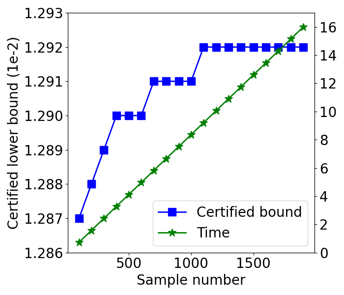
(a) Monte Carlo algorithm

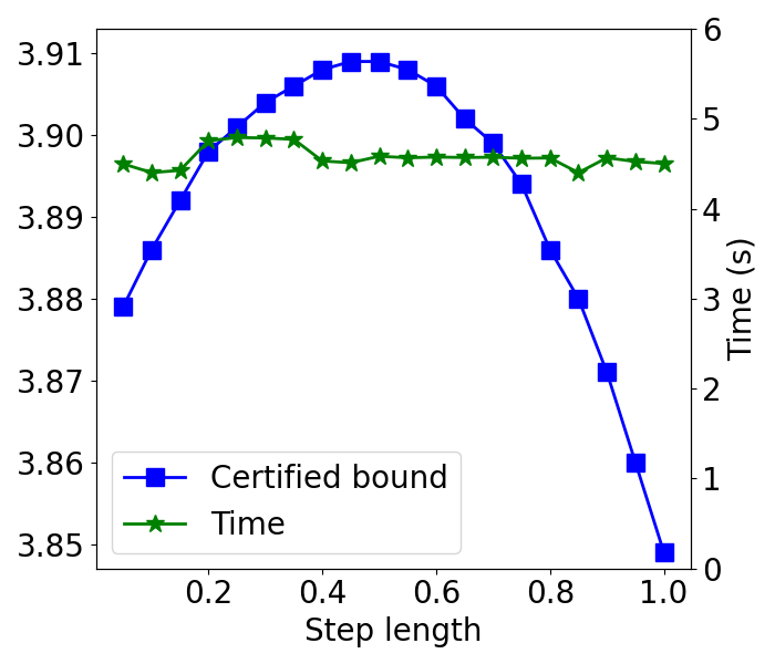
(b) Gradient-based algorithm

Figure 9. Exploring the influence of sample number and step length on certified lower bounds.

(a) FNNs on MNIST.

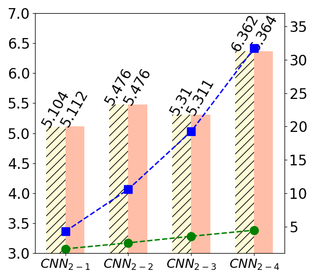
(b) CNNs on MNIST.

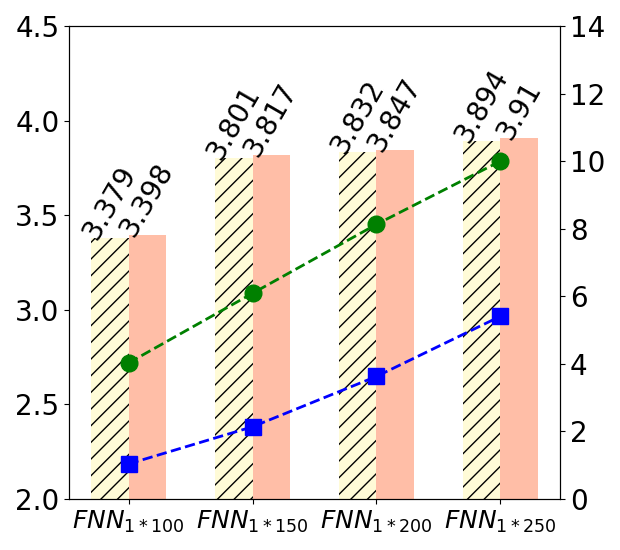
(c) FNNs on Fashion MNIST.

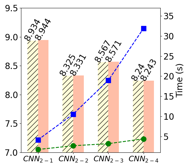
(d) FNNs on Fashion MNIST.

Figure 10. Comparison between the Monte Carlo and gradient-based algorithms for the robustness verification on 4 FNNs and 4 CNNs. The sample number is set to $1000$ while the step length to $0.45$.

Experiment II: Hyper-parameters. As approximation-based verification is intrinsically incomplete and the optimal values of hyper-parameters are unknowable, it is important to explore the hyper-parameter space for more effective and efficient verification. Hence, we measure the impacts of the two hyper-parameters, i.e., the sample number and the step length of gradient descent, in our Monte Carlo and gradient-based algorithms, respectively. They are quantitatively measured with respect to the certified lower bound and verification time. A larger lower bound implies a better hyper-parameter setting with respect to verification results.

We conduct the experiments on eight neural networks trained on MNIST and Fashion MNIST, respectively. Figure 9(a) shows the relation between certified lower bounds and the number of samples, resp. the time cost, for an FNN_1∗150 trained on Fashion MNIST. The computed bound is monotonously increasing with more samples, and stabilizes around $1000$ samples, which indicates that the under-approximation domain cannot be improved by simply running more simulations. Figure 9(b) shows the result of the gradient-based algorithm for the same FNN_1∗150. We consider the step length from $0.05\epsilon$ to $\epsilon$ by step of $0.05\epsilon$. It indicates that when the step length is set around $0.45\epsilon$, the computed bound is maximal.

As for the efficiency, we observe a linear relationship between the number of samples and the overhead for the Monte Carlo method. In contrast, the time cost is almost the same and independent of the step length. This conclusion is applicable to other networks and perturbation $\epsilon$. The complete experimental results are provided in Appendix C.2.

Experiment III: Monte Carlo vs. Gradient. We evaluate the performance of our two under-approximation algorithms. Figure 10 shows the certified lower bounds and the time cost of two algorithms on eight FNNs and eight CNNs with the Sigmoid activation function, respectively. We set the sample number to $1000$ and step length to $0.45$ (the optimal hyper-parameters from Experiment II). We observe that, compared to the Monte Carlo algorithm, the certified lower bounds computed by the gradient-based algorithm are always larger. The reason is that local information of neural network functions such as monotonicity can be obtained through gradients for computing more precise underestimated domains. This further demonstrates the usefulness of underestimated domains in defining tight over-approximations.

The experimental results also show that, the gradient-based algorithm costs less time on simple FNNs, while more time on complex CNNs. With small-sized neural networks, the gradient-based algorithm is faster as fewer steps are required in computing the gradient.

6. Related Work

This work is a sequel to existing efforts on approximation-based DNN robustness analysis. We classify them into two categories.

Over-approximation verification approaches. Due to the intrinsic complexity in the neural network robustness verification, approximating the non-linear activation functions is the mainstreaming approach for scalability. Zhang et al. defined three cases for over-approximating S-curved activation functions (Zhang et al., 2018). Wu and Zhang proposed a fine-grained approach and identified five cases for defining tighter approximations (Wu and Zhang, 2021). Lyu et al. proposed to define tight approximations by optimization at the price of sacrificing efficiency. Henriksen and Lomuscio (Henriksen and Lomuscio, 2020) defined tight approximations by minimizing the gap area between the bound and the curve. However, all these approaches are proved superior to others only on specific networks (Zhang et al., 2022b). The approximation approach in (Zhang et al., 2022b) is proved to be the tightest when the networks are monotonous. All these approaches only consider overestimated approximation domains, and thus they are superior to each other only on some selected network models. It is also unclear under what conditions these approaches except (Zhang et al., 2022b) are theoretically better than others. We believe that, the under-estimated domains could provide useful information to these approaches for defining tighter over-approximations.

Paulsen and Wang recently proposed an interesting approach for synthesizing tight approximations guided by generated examples (Paulsen and Wang, 2022a, b). Similar to our approach, these approaches compute sound and tight over-approximations from unsound templates. However, they require global optimization techniques to guarantee soundness, which is very time-consuming, while our approach ensures the soundness of individual neurons statistically.

Under-approximation analysis approaches. The essence of our dual approximation approach is to underestimate activation functions’ domains for guiding the definition of tight over-approximations. There are several related under-approximation approaches based on either white-box attacks (Chakraborty et al., 2018) or testings (He et al., 2022). For instance, the fast gradient sign method (FGSM) (Goodfellow et al., 2015) is a well-known approach for generating adversarial examples to intrigue corner cases for classifications. Other attack approaches include C&W (Carlini and Wagner, 2017), DeepFool (Moosavi-Dezfooli et al., 2016), and JSMA (Papernot et al., 2016). The white-box testing for neural networks is to generate specific test cases to intrigue target neurons under different coverage criteria. Various test case generation and selection approaches have been proposed (Lee et al., 2020a; Sun et al., 2019; Yu et al., 2022; Guo et al., 2018; Gao et al., 2022). We believe that our approach provides a flexible hybrid mechanism to combine these attack- and testing-based under-approximation approaches into over-approximation-based verification approaches for neural network robustness verification. These sophisticated attack and testing approaches can be used for underestimating the approximation domains. We would consider integrating them into our dual-approximation approach for the improvement of both tightness and efficiency.

7. Conclusion

We have proposed a dual-approximation approach to define tight over-approximations for the robustness verification of DNNs. Underlying this approach is our finding of approximation domain of the activation function that is crucial in defining tight over-approximations, yet overlooked by all existing approximation approaches. Accordingly, we have devised two complementary under-approximation algorithms to compute underestimated domains, which are proved to be useful to define tight over-approximations for neural networks. Based on this, we proposed a novel dual-approximation approach to define tight over-approximations via the additional underestimated domain of activation functions. Our experimental results have demonstrated the outperformance of our approach over the state of the art.

Our dual-approximation approach sheds light on a new direction at integrating under-approximation approaches such as attacks and testings into over-approximation-based verification approaches for neural networks. Besides, it could also be integrated into other abstraction-based neural network verification approaches (Gehr et al., 2018; Singh et al., 2019; Zhang et al., 2020) as they require non-linear activation functions that shall be over-approximated to handle abstract domains. In addition to the robustness verification, we believe that our approach is also applicable to the variants of robustness verification problems, such as fairness (Bastani et al., 2019) and $\epsilon$-weekend robustness (Huang et al., 2022). Verifying those properties can be reduced to optimization problems that contain the nonlinear activation functions in networks.

Appendix A The Proofs of Theorems

In this section, we give the proof of Theorem 3.2 and Theorem 3.3 proposed in Section 3.3.

A.1. Proof of Theorem 3.2

Theorem A.1 (3.1).

Suppose that there are two over-approximations $h_{L}(z^{(j)}(x)),h_{U}(z^{(j)}(x))$ and ${h^{\prime}}_{L}(z^{(j)}(x)),{h^{\prime}}_{U}(z^{(j)}(x))$ for each $z^{(j)}(x)$ in Definition 3.1 and $h_{L}(z^{(j)}(x)),h_{U}(z^{(j)}(x))$ are tighter than ${h^{\prime}}_{L}(z^{(j)}(x)),{h^{\prime}}_{U}(z^{(j)}(x))$, respectively. The approximation domain $[l_{r}^{(i)},u_{r}^{(i)}]$ computed by $h_{L}(z^{(j)}(x)),h_{U}(z^{(j)}(x))$ must be more precise than the one $[{l^{\prime}}_{r}^{(i)},{u^{\prime}}_{r}^{(i)}]$ by ${h^{\prime}}_{L}(z^{(j)}(x)),{h^{\prime}}_{U}(z^{(j)}(x))$.

Proof.

Assume that there is a neuron $N_{i}$ with m neurons $N_{1}$, $N_{2}$, $\cdots$, $N_{m}$ connected to it on the last layer. There are two over-approximation methods, one of which is tighter than the other. For $N_{i}$, the tighter approximated output of it is $[l_{i},u_{i}]$, and the looser is $[l^{\prime}_{i},u^{\prime}_{i}]$ where $l^{\prime}_{i}\leq l_{i}$ and $u_{i}\leq u^{\prime}_{i}$. For $N_{1}$, $N_{2}$, $\cdots$, $N_{m}$, they are $[l_{1},u_{1}]$, $[l_{2},u_{2}]$, $\cdots$, $[l_{m},u_{m}]$ and $[l^{\prime}_{1},u^{\prime}_{1}]$, $[l^{\prime}_{2},u^{\prime}_{2}]$, $\cdots$, $[l^{\prime}_{m},u^{\prime}_{m}]$, respectively. Let $w_{1}$, $w_{2}$, $\cdots$, $w_{m}$ and $b_{1}$, $b_{2}$, $\cdots$, $b_{m}$ be the weights of biases of the connection between $N_{i}$ and $N_{1}$, $N_{2}$, $\cdots$, $N_{m}$. We consider three cases where the weights are positive or negative:

Case I: All weights are positive. If $w_{1},w_{2},\cdots,w_{m}>0$, then the approximation domains of $N_{i}$ are $[l_{i},u_{i}]$ and $[l^{\prime}_{i},u^{\prime}_{i}]$ where

$$l_{i}= \enspace w_{1}l_{1}+w_{2}l_{2}+\cdots+w_{m}l_{m}+b_{1}+b_{2}+\cdots+b_{m}$$

$$u_{i}= \enspace w_{1}u_{1}+w_{2}u_{2}+\cdots+w_{m}u_{m}+b_{1}+b_{2}+\cdots+b_{m}$$

$$l^{\prime}_{i}= \enspace w_{1}l^{\prime}_{1}+w_{2}l^{\prime}_{2}+\cdots+w_{m}l^{\prime}_{m}+b_{1}+b_{2}+\cdots+b_{m}$$

$$u^{\prime}_{i}= \enspace w_{1}u^{\prime}_{1}+w_{2}u^{\prime}_{2}+\cdots+w_{m}u^{\prime}_{m}+b_{1}+b_{2}+\cdots+b_{m}$$

Clearly, $l_{i}\geq l^{\prime}_{i}$ and $u_{i}\leq u^{\prime}_{i}$. We know that $[l_{i},u_{i}]$ is tighter than $[l^{\prime}_{i},u^{\prime}_{i}]$.

Case II: $m-1$ weights are positive. If $w_{1},w_{2},\cdots,w_{m-1}>0$ and $w_{m}\leq 0$, then:

$$l_{i}= \enspace w_{1}l_{1}+w_{2}l_{2}+\cdots+w_{m-1}l_{m-1}+w_{m}u_{m}+$$

$$\enspace b_{1}+b_{2}+\cdots+b_{m}$$

$$u_{i}= \enspace w_{1}u_{1}+w_{2}u_{2}+\cdots+w_{m-1}u_{m-1}+w_{m}l_{m}+$$

$$\enspace b_{1}+b_{2}+\cdots+b_{m}$$

$$l^{\prime}_{i}= \enspace w_{1}l^{\prime}_{1}+w_{2}l^{\prime}_{2}+\cdots+w_{m-1}l^{\prime}_{m-1}+w_{m}u^{\prime}_{m}+$$

$$\enspace b_{1}+b_{2}+\cdots+b_{m}$$

$$u^{\prime}_{i}= \enspace w_{1}u^{\prime}_{1}+w_{2}u^{\prime}_{2}+\cdots+w_{m-1}u^{\prime}_{m-1}+w_{m}l^{\prime}_{m}+$$

$$\enspace b_{1}+b_{2}+\cdots+b_{m}$$

Since $l_{1}\geq l^{\prime}_{1}$, $l_{2}\geq l^{\prime}_{2}$, $\cdots$, $l_{m-1}\leq l^{\prime}_{m-1}$ and $u_{m}\leq u^{\prime}_{m}$, we have $l_{i}\geq l^{\prime}_{i}$. Similarly, $u_{i}\leq u^{\prime}_{i}$, and then $[l_{i},u_{i}$ is tighter than $[l^{\prime}_{i},u^{\prime}_{i}]$.

Case III: No weights are positive. If $w_{1},w_{2},\cdots.w_{m}<=0$, then:

$$l_{i}= \enspace w_{1}u_{1}+w_{2}u_{2}+\cdots+w_{m}u_{m}+b_{1}+b_{2}+\cdots+b_{m}$$

$$u_{i}= \enspace w_{1}l_{1}+w_{2}l_{2}+\cdots+w_{m}l_{m}+b_{1}+b_{2}+\cdots+b_{m}$$

$$l^{\prime}_{i}= \enspace w_{1}u^{\prime}_{1}+w_{2}u^{\prime}_{2}+\cdots+w_{m}u^{\prime}_{m}+b_{1}+b_{2}+\cdots+b_{m}$$

$$u^{\prime}_{i}= \enspace w_{1}l^{\prime}_{1}+w_{2}l^{\prime}_{2}+\cdots+w_{m}l^{\prime}_{m}+b_{1}+b_{2}+\cdots+b_{m}$$

Clearly, $l_{i}\geq l^{\prime}_{i}$ and $u_{i}\leq u^{\prime}_{i}$, and then $[l_{i},u_{i}$ is tighter than $[l^{\prime}_{i},u^{\prime}_{i}]$.

From the three cases above, we can conclude that whether the weights $w$ of connection between two neurons are positive or non-positive, and regardless of the biases $b$, if the over-approximation is tighter, the approximation domain of neurons in the next layer will be more precise. ∎

A.2. Proof of Theorem 3.3

Theorem A.2 (3.2).

Given two approximation domains $[l_{r}^{(i)},u_{r}^{(i)}]$ and $[{l^{\prime}}_{r}^{(i)},{u^{\prime}}_{r}^{(i)}]$ such that ${l^{\prime}}_{r}^{(i)}<l_{r}^{(i)}$ and $u_{r}^{(i)}<{u^{\prime}}_{r}^{(i)}]$, for any over-approximation $({h^{\prime}}_{L}(z^{(j)}(x)),{h^{\prime}}_{U}(z^{(j)}(x)))$ of continuous function $\sigma(x)$ on $[{l^{\prime}}_{r}^{(i)},{u^{\prime}}_{r}^{(i)}]$, there exists an over-approximation $(h_{L}(z^{(j)}(x))$, $h_{U}(z^{(j)}(x)))$ on $[l_{r}^{(i)},u_{r}^{(i)}]$ such that $\forall z^{(j)}(x)\in[l_{r}^{(i)},u_{r}^{(i)}],h^{\prime}_{L}(x)\leq h_{L}(z^{(j)}(x)),h^{\prime}_{U}(x)\geq h_{U}(z^{(j)}(x))$.

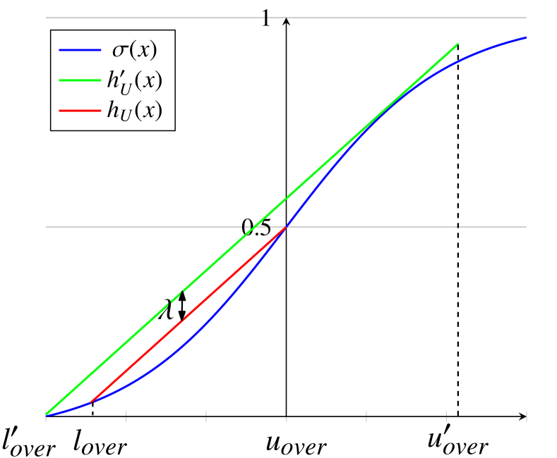
(a) $h_{U}(x)=h^{\prime}_{U}(x)-\lambda$

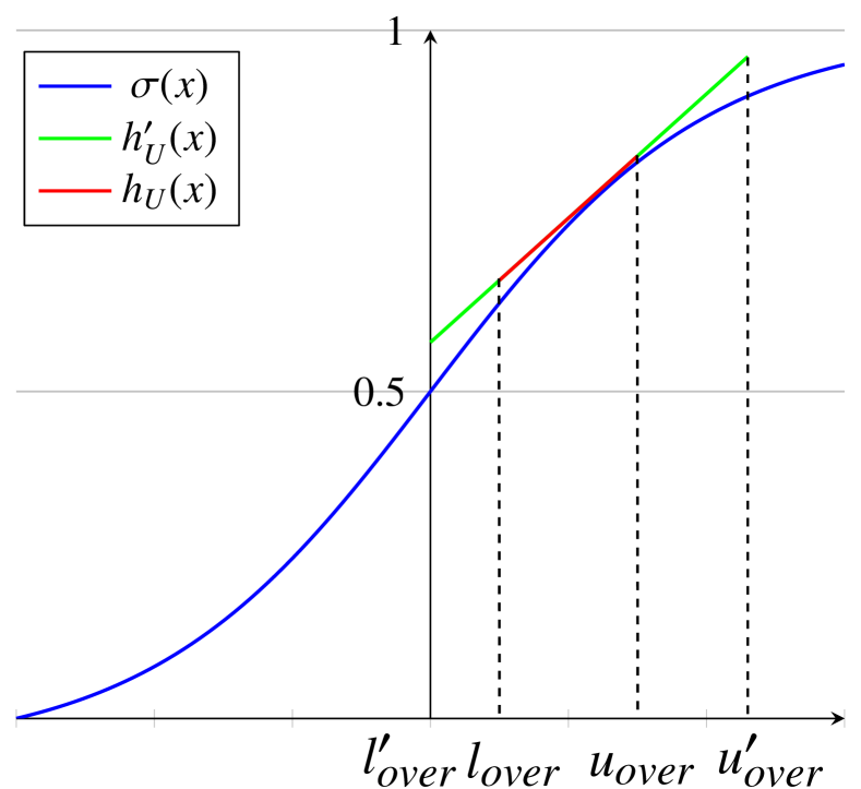
(b) $h_{U}(x)=h^{\prime}_{U}(x)$

Figure 11. Two cases of defining $h_{U}(x)$ based on $h^{\prime}_{U}(x)$

Proof.

To simplify, We omit superscript and subscript and use $[l_{over},u_{over}]$ and $[l^{\prime}_{over},u^{\prime}_{over}]$ to denote the overestimated approximation domains. Since we have $l^{\prime}_{over}<l_{over}$ and $u_{over}<u^{\prime}_{over}$, which means $[l_{over},u_{over}]\subset[l^{\prime}_{\mathit{over}},u^{\prime}_{\mathit{over}}]$, and $\sigma$ is a continuous function, we can conclude that the range of $\sigma$ satisfies: $\sigma([l_{\mathit{over}},u_{\mathit{over}}])\subset\sigma([l^{\prime}_{\mathit{over}},u^{\prime}_{\mathit{over}}])$. Given the linear upper bound $h^{\prime}_{U}(x)$ on $[l^{\prime}_{over},u^{\prime}_{over}]$, we can define a linear upper bound $h_{U}(x)$ on $[l_{over},u_{over}]$ as:

(7) $$h_{U}(x)=\begin{cases}h^{\prime}_{U}(x)-\lambda&\mathit{if}~{}\forall x\in[l_{over},u_{over}],\exists\lambda>0,\\ &\quad h^{\prime}_{U}(x)-\sigma(x)\geq\lambda\\ h^{\prime}_{U}(x)&\mathit{otherwise}\end{cases}$$

The two cases above are intuitively shown in Figure 11. Apparently, $h_{U}(x)$ is tighter than $h^{\prime}_{U}(x)$ since $h_{U}(x)\leq h^{\prime}_{U}(x)$.

Now we show that $h_{U}(x)$ is a sound upper bound for $\sigma$ on $[l_{over},u_{over}]$. That is, for all $x$ in $[l_{over},u_{over}]$, if $h_{U}(x)=h^{\prime}_{U}(x)-\lambda$, then $h_{U}(x)-\sigma(x)=h^{\prime}_{U}(x)-\lambda-\sigma(x)$. Since $h^{\prime}_{U}(x)-\sigma(x)\geq\lambda$, we have $h_{U}(x)-\sigma(x)\geq 0$, and in this case $h_{U}(x)$ is sound. Moreover, if $h_{U}(x)=h^{\prime}_{U}(x)$, since $h^{\prime}_{U}(x)$ is a linear upper bound, $h^{\prime}_{U}(x)\geq\sigma(x)$, and $h_{U}(x)\geq\sigma(x)$. For the linear lower bound, the proof is similar. We can conclude that more precise approximation domains lead to tighter over-approximations of activation functions. ∎

Appendix B Soundness of Our Approach

We demonstrate the soundness of our dual-approximation approach. For non-linear functions $\sigma(x)$, we first underestimate its actual domain using Monte Carlo or gradient-based approaches, and then over-approximate it on both the underestimated domain and the overestimated domain. The over-approximation strategy computes $h_{L}(x)$ and $h_{U}(x)$ for each case. We prove that our approach is sound by showing $\forall x\in[l_{over},u_{over}],h_{L}(x)\leq\sigma(x)\leq h_{U}(x)$.

Theorem B.1.

The dual-approximation approach is sound.

Proof.

Consider the three cases defined in Section 4.3. In case I, the linear upper bound $h_{U}(x)=k(x-u_{over})+\sigma(u_{over})$. Let $f(x)=h_{U}(x)-\sigma(x)$, we show $h_{U}(x)$ is sound by proving $f(x)\geq 0$. The derivative of $f(x)$ is $f^{\prime}(x)=k-\sigma^{\prime}(x)$.

If $l_{over},u_{over}<0$, as $\sigma^{\prime}(l_{over})<k<\sigma^{\prime}(u_{over})$ and $\sigma(x)$ is monotonically increasing, there must exists $x_{0}\in(l_{over},u_{over})$ where $\sigma^{\prime}(x_{0})=k$. When $x\in[l_{over},x_{0}]$, $f^{\prime}(x)>0$, and $f(x)$ is monotonically increasing; when $x\in[x_{0},u_{over}]$, $f^{\prime}(x)<0$, and $f(x)$ is monotonically decreasing. The two minimum occurs at $l_{over}$ and $u_{over}$. Since $f(l_{over})=f(u_{over})=0$, we can conclude that $f(x)\geq 0$.

If $l_{over}<0$ and $u_{over}>0$, we divide $[l_{over},u_{over}]$ into $[l_{over},0]$ and $[0,u_{over}]$, and consider them separately. For $x\in[l_{over},0]$, the case is similar to the above. There exists some $x_{0}$ where $f^{\prime}(x_{0})=0$. $f(x)$ is monotonically increasing in $[l_{over},x_{0}]$, and monotonically decreasing in $[x_{0},0]$. For $x\in[0,u_{over}]$, as $k<\sigma^{\prime}(u_{over})$ and $\sigma(x)$ is monotonically decreasing, we know that $f^{\prime}(x)<0$, and $f(x)$ is monotonically decreasing in $[0,u_{over}]$. All in all, $f(x)$ is monotonically increasing in $[l_{over},x_{0}]$, and monotonically decreasing in $[x_{0},u_{over}]$. The two minimum occurs at $l_{over}$ and $u_{over}$. Since $f(l_{over})=f(u_{over})=0$, we know that $f(x)\geq 0$.

The condition where $l_{over},u_{over}>0$ is nonexistent in this case.

In the proof above, we show that $\forall x\in[l_{over},u_{over}]$, the upper bound $h_{U}(x)\geq\sigma(x)$, and thus it is sound. As for the lower bound $h_{L}(x)$, as well as Case II and III, the proof is similar. ∎

Appendix C Additional Experimental Results

Table 3. Additional Comparison result I: Comparison of Monte-Carlo-version DualApp (DA) and existing tools, NeWise (NW), DeepCert (DC), VeriNet (VN) and RobustVerifier (RV) on 16 Sigmoid networks.

Database	Model	Nodes	DA	NW	Impr. (%)	DC	Impr. (%)	VN	Impr. (%)	RV	Impr. (%)	DA Time (s)	Others Time(s)
			Bounds	Bounds		Bounds		Bounds		Bounds
Mnist	${\rm CNN}_{3-2}$	2,514	0.06119	0.06074	0.74	0.05789	5.70	0.05803	5.45	0.05686	7.62	2.81	0.15 ±0.02
	${\rm CNN}_{3-4}$	5018	0.04875	0.04776	2.07	0.04721	3.26	0.04715	3.39	0.04639	5.09	3.44	0.15 ±0.02
	${\rm CNN}_{4-5}$	8690	0.04863	0.04763	2.10	0.04551	6.86	0.04548	6.93	0.04355	11.66	15.33	0.89 ±0.03
	${\rm FNN}_{3\times 50}$	160	0.00779	0.00693	12.41	0.0076	2.50	0.00768	1.43	0.00649	20.03	3.28	0.15 ±0.02
	${\rm FNN}_{3\times 100}$	310	0.00885	0.00777	13.90	0.00858	3.15	0.00871	1.61	0.00744	18.95	5.46	0.22 ±0.02
Fashion Mnist	${\rm CNN}_{3-2}$	2,514	0.03006	0.02839	5.88	0.02584	16.33	0.02930	2.59	0.02811	6.94	2.86	0.15 ±0.01
	${\rm CNN}_{3-4}$	5,018	0.03430	0.03125	9.76	0.03084	11.22	0.03390	1.18	0.03094	10.86	5.92	0.28 ±0.03
	${\rm FNN}_{3\times 50}$	160	0.00574	0.00476	20.59	0.00447	28.41	0.00565	1.59	0.00476	20.59	3.15	0.14 ±0.01
	${\rm FNN}_{3\times 100}$	310	0.00497	0.00391	27.11	0.00387	28.42	0.00490	1.43	0.00471	5.52	5.32	0.42 ±0.08
	${\rm FNN}_{3\times 400}$	1210	0.00442	0.00312	41.67	0.00322	37.27	0.00437	1.14	0.00355	24.51	25.22	4.20 ±0.21
	${\rm FNN}_{3\times 700}$	2,110	0.00408	0.00284	43.66	0.00290	40.69	0.00401	1.75	0.00318	28.30	50.12	12.14 ±0.39
Cifar-10	${\rm CNN}_{3-4}$	5,018	0.01136	0.01064	6.77	0.01067	6.47	0.01133	0.26	0.01118	1.61	4.87	0.28 ±0.03
	${\rm CNN}_{4-5}$	8690	0.01942	0.01863	4.24	0.01917	1.30	0.01912	1.57	0.01887	2.91	17.22	1.17 ±0.08
	${\rm FNN}_{3\times 50}$	160	0.00455	0.00406	12.07	0.00454	0.22	0.00452	0.66	0.00415	9.64	6.68	2.07 ±0.26
	${\rm FNN}_{3\times 100}$	310	0.00469	0.00401	16.96	0.00468	0.21	0.00466	0.64	0.00426	10.09	12.23	3.98±0.84
	${\rm FNN}_{3\times 200}$	610	0.00408	0.00344	18.60	0.00407	0.25	0.00406	0.49	0.00377	8.22	30.27	12.82 ±2.11

Table 4. Additional Comparison result II: Comparison results of Monte-Carlo-version DualApp (DA) and existing tools, NeWise (NW), DeepCert (DC), VeriNet (VN), and RobustVerifier (RV) on 16 Tanh networks.

Database	Model	Nodes	DA	NW	Impr. (%)	DC	Impr. (%)	VN	Impr. (%)	RV	Impr. (%)	DA Time (s)	Others Time(s)
			Bounds	Bounds		Bounds		Bounds		Bounds
Mnist	${\rm CNN}_{3-2}$	2,514	0.02677	0.02558	4.65	0.02618	2.25	0.02622	2.10	0.02565	4.37	3.34	0.16 ±0.02
	${\rm FNN}_{3\times 50}$	160	0.00545	0.00456	19.52	0.00529	3.02	0.00536	1.68	0.00439	24.15	3.02	0.14 ±0.00
	${\rm FNN}_{3\times 100}$	310	0.00623	0.00499	24.85	0.00609	2.30	0.00616	1.14	0.00512	21.68	5.28	0.37 ±0.01
	${\rm FNN}_{3\times 200}$	610	0.00676	0.00508	33.07	0.00663	1.96	0.00669	1.05	0.00557	21.36	10.42	1.19 ±0.05
	${\rm FNN}_{3\times 400}$	1,210	0.00672	0.00479	40.29	0.00660	1.82	0.00667	0.75	0.00553	21.52	24.28	4.63 ±0.12
	${\rm FNN}_{3\times 700}$	2,110	0.00665	0.00459	44.88	0.00650	2.31	0.00660	0.76	0.00537	23.84	50.48	12.27 ±0.43
Fashion Mnist	${\rm CNN}_{3-2}$	2514	0.09247	0.09091	1.72	0.08805	5.02	0.08772	5.41	0.08387	10.25	3.22	0.15 ±0.02
	${\rm CNN}_{3-4}$	5018	0.07704	0.07452	3.38	0.0729	5.68	0.07295	5.61	0.06848	12.50	5.68	0.26 ±0.05
	${\rm FNN}_{3\times 50}$	160	0.01035	0.00915	13.11	0.01013	2.17	0.0102	1.47	0.00858	20.63	3.87	0.20 ±0.01
	${\rm FNN}_{3\times 100}$	310	0.00921	0.00797	15.56	0.00907	1.54	0.00911	1.10	0.00778	18.38	6.33	0.57 ±0.12
	${\rm FNN}_{3\times 700}$	2,110	0.00757	0.00634	19.40	0.00749	1.07	0.00751	0.80	0.00666	13.66	78.02	13.44 ±0.62
Cifar-10	${\rm CNN}_{3-4}$	5018	0.02551	0.02469	3.32	0.02528	0.91	0.02523	1.11	0.02492	2.37	6.02	0.26 ±0.05
	${\rm CNN}_{4-5}$	8690	0.01942	0.01863	4.24	0.01917	1.30	0.01912	1.57	0.01887	2.91	7.79	1.73 ±0.24
	${\rm FNN}_{3\times 50}$	160	0.00287	0.00232	23.71	0.00285	0.70	0.00285	0.70	0.00254	12.99	7.79	1.73 ±0.24
	${\rm FNN}_{3\times 100}$	310	0.00253	0.00194	30.41	0.00251	0.80	0.00251	0.80	0.00225	12.44	19.47	10.45 ±4.36
	${\rm FNN}_{3\times 700}$	2,110	0.00229	0.00155	47.74	0.00226	1.33	0.00228	0.44	0.00201	13.93	122.89	66.01 ±12.74

Table 5. Additional Comparison results III: Comparison of Monte-Carlo-version DualApp (DA) and existing tools, NeWise (NW), DeepCert (DC), VeriNet (VN) and RobustVerifier (RV) on 18 Arctan networks.

Database	Model	Nodes	DA	NW	Impr. (%)	DC	Impr. (%)	VN	Impr. (%)	RV	Impr. (%)	DA	Others Time(s)
			Bounds	Bounds		Bounds		Bounds		Bounds
Mnist	${\rm CNN}_{3-2}$	2,514	0.01920	0.01821	5.44	0.01836	4.58	0.01896	1.27	0.01829	4.98	2.78	0.15 ±0.02
	${\rm FNN}_{3\times 50}$	160	0.00568	0.00481	18.09	0.00437	29.98	0.00558	1.79	0.00465	22.15	3.02	0.16 ±0.02
	${\rm FNN}_{3\times 100}$	310	0.00635	0.00518	22.59	0.00495	28.28	0.00627	1.28	0.00529	20.04	5.11	0.37 ±0.04
	${\rm FNN}_{3\times 200}$	610	0.00716	0.00547	30.90	0.00554	29.24	0.00708	1.13	0.00587	21.98	10.34	1.20 ±0.02
	${\rm FNN}_{3\times 400}$	1,210	0.00733	0.00528	38.83	0.00551	33.03	0.00725	1.10	0.00589	24.45	25.46	4.65 ±0.42
	${\rm FNN}_{3\times 700}$	2,110	0.00721	0.00506	42.49	0.00532	35.53	0.00713	1.12	0.00572	26.05	50.98	12.18 ±0.23
Fashion Mnist	${\rm CNN}_{3-2}$	2,514	0.03006	0.02839	5.88	0.02584	16.33	0.02930	2.59	0.02811	6.94	2.86	0.15 ±0.01
	${\rm CNN}_{3-4}$	5,018	0.03430	0.03125	9.76	0.03084	11.22	0.03390	1.18	0.03094	10.86	5.92	0.28 ±0.03
	${\rm FNN}_{3\times 50}$	160	0.00574	0.00476	20.59	0.00447	28.41	0.00565	1.59	0.00476	20.59	3.15	0.14 ±0.01
	${\rm FNN}_{3\times 100}$	310	0.00497	0.00391	27.11	0.00387	28.42	0.00490	1.43	0.00471	5.52	5.32	0.42 ±0.08
	${\rm FNN}_{3\times 200}$	610	0.00471	0.00349	34.96	0.00358	31.56	0.00466	1.07	0.00390	20.77	10.56	1.20 ±0.06
	${\rm FNN}_{3\times 400}$	1210	0.00442	0.00312	41.67	0.00322	37.27	0.00437	1.14	0.00355	24.51	25.22	4.20 ±0.21
	${\rm FNN}_{3\times 700}$	2,110	0.00408	0.00284	43.66	0.00290	40.69	0.00401	1.75	0.00318	28.30	50.12	12.14 ±0.39
Cifar-10	${\rm CNN}_{3-4}$	5,018	0.01136	0.01064	6.77	0.01067	6.47	0.01133	0.26	0.01118	1.61	4.87	0.28 ±0.03
	${\rm FNN}_{3\times 50}$	160	0.00323	0.00262	23.28	0.00266	21.43	0.00321	0.62	0.00283	14.13	7.26	1.67 ±0.16
	${\rm FNN}_{3\times 100}$	310	0.00277	0.00216	28.24	0.00220	25.91	0.00275	0.73	0.00248	11.69	13.88	4.33±0.88
	${\rm FNN}_{3\times 200}$	610	0.00255	0.00189	34.92	0.00196	30.10	0.00253	0.79	0.00228	11.84	27.94	10.48 ±1.56
	${\rm FNN}_{3\times 700}$	2,110	0.00246	0.00167	47.31	0.00179	37.43	0.00245	0.41	0.00212	16.04	79.10	36.44 ±3.85

C.1. Additional Results for Experiment I

This section presents the effectiveness comparison of DualApp with NeWise, DeepCert, VeriNet, and RobustVerifier on additional 16 Sigmoid, 16 Tanh, and 18 Arctan neural networks. The results are shown in Table 3, 4, and 5 respectively. All the experiments clearly show that our method outperforms our competitors on all datasets and models.

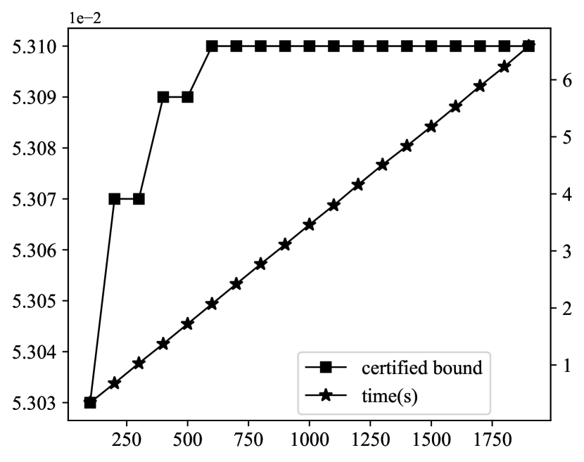
(a) Sampling-based results on $\rm{CNN}_{2-3}$ trained on Mnist.

(b) Sampling-based results on $\rm{FNN}_{1\times 200}$ trained on Mnist.

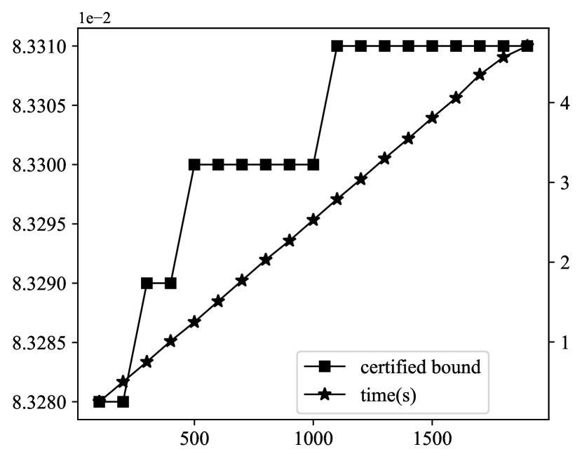
(c) Sampling-based results on $\rm{CNN}_{2-2}$ trained on Fashion Mnist.

(d) Gradient-based results on $\rm{CNN}_{2-3}$ trained on Mnist.

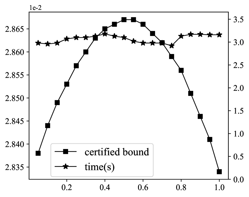
(e) Gradient-based results on $\rm{FNN}_{1\times 200}$ trained on Mnist.

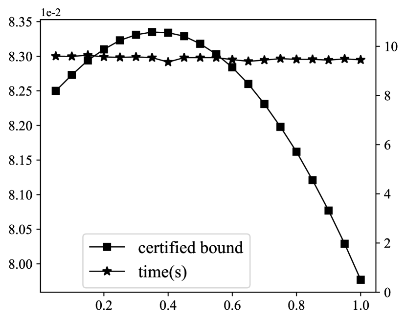
(f) Gradient-based results on $\rm{CNN}_{2-2}$ trained on Fashion Mnist.

Figure 12. Additional Experimental results: The effect of hyper-parameters in the Monte Carlo and gradient-based algorithms. The main coordinate denotes certified bounds and the second coordinate denotes the time consumed.

C.2. Additional Results for Experiment III

This section presents additional results on the exploration of hyper-parameters in the Monte Carlo algorithm and gradient-based algorithm. The results are shown in Figure 12. In the Monte Carlo algorithm, the computed certified lower bounds are maximal when the sample number is around 1000. In the gradient-based algorithm, they are maximal when the step length is around $0.45\epsilon$. All these experiments are consistent with our conclusions in the text.

References

- (1)
- Apollo (2017) Apollo. 2017. ApolloAuto. https://github.com/ApolloAuto/apollo. Accessed: 2022-05-06.
- Bastani et al. (2019) Osbert Bastani, Xin Zhang, and Armando Solar-Lezama. 2019. Probabilistic verification of fairness properties via concentration. Proc. ACM Program. Lang. 3 (2019), 118:1–118:27.
- Bojarski et al. (2016) Mariusz Bojarski, Davide Del Testa, Daniel Dworakowski, Bernhard Firner, Beat Flepp, Prasoon Goyal, Lawrence D. Jackel, Mathew Monfort, Urs Muller, Jiakai Zhang, Xin Zhang, Jake Zhao, and Karol Zieba. 2016. End to End Learning for Self-Driving Cars. CoRR abs/1604.07316 (2016).
- Carlini and Wagner (2017) Nicholas Carlini and David A. Wagner. 2017. Towards Evaluating the Robustness of Neural Networks. In IEEE Symposium on Security and Privacy (S&P’17). 39–57.
- Chakraborty et al. (2018) Anirban Chakraborty, Manaar Alam, Vishal Dey, Anupam Chattopadhyay, and Debdeep Mukhopadhyay. 2018. Adversarial Attacks and Defences: A Survey. CoRR abs/1810.00069 (2018).
- Elboher et al. (2020) Yizhak Yisrael Elboher, Justin Gottschlich, and Guy Katz. 2020. An abstraction-based framework for neural network verification. In International Conference on Computer Aided Verification (CAV’20). Springer, 43–65.
- Gao et al. (2022) Xinyu Gao, Yang Feng, Yining Yin, Zixi Liu, Zhenyu Chen, and Baowen Xu. 2022. Adaptive Test Selection for Deep Neural Networks. In IEEE/ACM International Conference on Software Engineering (ICSE’22). ACM, 73–85.
- Gehr et al. (2018) Timon Gehr, Matthew Mirman, Dana Drachsler-Cohen, Petar Tsankov, Swarat Chaudhuri, and Martin Vechev. 2018. AI2: Safety and Robustness Certification of Neural Networks with Abstract Interpretation. In IEEE Symposium on Security and Privacy (S&P’18). IEEE, 3–18.
- Goodfellow et al. (2015) Ian J. Goodfellow, Jonathon Shlens, and Christian Szegedy. 2015. Explaining and Harnessing Adversarial Examples. In International Conference on Learning Representations (ICLR’15).
- Guo et al. (2018) Jianmin Guo, Yu Jiang, Yue Zhao, Quan Chen, and Jiaguang Sun. 2018. DLFuzz: differential fuzzing testing of deep learning systems. In ACM Joint European Software Engineering Conference and Symposium on the Foundations of Software Engineering (ESEC/FSE’18). 739–743.
- He et al. (2022) Yingzhe He, Guozhu Meng, Kai Chen, Xingbo Hu, and Jinwen He. 2022. Towards Security Threats of Deep Learning Systems: A Survey. IEEE Trans. Software Eng. 48 (2022), 1743–1770.
- Henriksen and Lomuscio (2020) Patrick Henriksen and Alessio Lomuscio. 2020. Efficient Neural Network Verification via Adaptive Refinement and Adversarial Search. In European Association for Artificial Intelligence (ECAI’20). 2513–2520.
- Huang et al. (2019) Po-Sen Huang, Robert Stanforth, Johannes Welbl, Chris Dyer, Dani Yogatama, Sven Gowal, Krishnamurthy Dvijotham, and Pushmeet Kohli. 2019. Achieving Verified Robustness to Symbol Substitutions via Interval Bound Propagation. In Conference on Empirical Methods in Natural Language Processing and 9th International Joint Conference on Natural Language Processing EMNLP-IJCNLP’19. 4081–4091.
- Huang et al. (2022) Pei Huang, Yuting Yang, Minghao Liu, Fuqi Jia, Feifei Ma, and Jian Zhang. 2022. -weakened robustness of deep neural networks. In International Symposium on Software Testing and Analysis (ISSTA’22). 126–138.
- Huang et al. (2020) Xiaowei Huang, Daniel Kroening, Wenjie Ruan, James Sharp, Youcheng Sun, Emese Thamo, Min Wu, and Xinping Yi. 2020. A survey of safety and trustworthiness of deep neural networks: Verification, testing, adversarial attack and defence, and interpretability. Comput. Sci. Rev. 37 (2020), 100270.
- Ilyas et al. (2019) Andrew Ilyas, Shibani Santurkar, Dimitris Tsipras, Logan Engstrom, Brandon Tran, and Aleksander Madry. 2019. Adversarial Examples Are Not Bugs, They Are Features. In Advances in Neural Information Processing Systems (NeurIPS’19). 125–136.
- Katz et al. (2017) Guy Katz, Clark Barrett, David L Dill, Kyle Julian, and Mykel J Kochenderfer. 2017. Reluplex: An Efficient SMT Solver for Verifying Deep Neural Networks. In International Conference on Computer Aided Verification (CAV’17). Springer, 97–117.
- Krizhevsky et al. (2009) Alex Krizhevsky, Geoffrey Hinton, et al. 2009. Learning Multiple Layers of Features from Tiny Images. (2009).
- LeCun et al. (1998) Yann LeCun, Léon Bottou, Yoshua Bengio, and Patrick Haffner. 1998. Gradient-based learning applied to document recognition. Proc. IEEE 86 (1998), 2278–2324.
- Lee et al. (2020a) Seokhyun Lee, Sooyoung Cha, Dain Lee, and Hakjoo Oh. 2020a. Effective white-box testing of deep neural networks with adaptive neuron-selection strategy. In ACM SIGSOFT International Symposium on Software Testing and Analysis (ISSTA’20). 165–176.
- Lee et al. (2020b) Sungyoon Lee, Jaewook Lee, and Saerom Park. 2020b. Lipschitz-Certifiable Training with a Tight Outer Bound. In NeurIPS’20. 16891–16902.
- Lin et al. (2019) Wang Lin, Zhengfeng Yang, Xin Chen, Qingye Zhao, Xiangkun Li, Zhiming Liu, and Jifeng He. 2019. Robustness Verification of Classification Deep Neural Networks via Linear Programming. In IEEE/CVF Conference on Computer Vision and Pattern Recognition (CVPR’19). 11418–11427.
- Liu et al. (2021) Changliu Liu, Tomer Arnon, Christopher Lazarus, Christopher A. Strong, Clark W. Barrett, and Mykel J. Kochenderfer. 2021. Algorithms for Verifying Deep Neural Networks. Found. Trends Optim. 4 (2021), 244–404.
- Liu et al. (2022) Zixi Liu, Yang Feng, Yining Yin, and Zhenyu Chen. 2022. DeepState: Selecting Test Suites to Enhance the Robustness of Recurrent Neural Networks. In IEEE/ACM International Conference on Software Engineering (ICSE’22). 598–609.
- Lyu et al. (2020) Zhaoyang Lyu, Ching-Yun Ko, Zhifeng Kong, Ngai Wong, Dahua Lin, and Luca Daniel. 2020. Fastened CROWN: Tightened Neural Network Robustness Certificates. In AAAI Conference on Artificial Intelligence (AAAI’20). 5037–5044.
- Moosavi-Dezfooli et al. (2016) Seyed-Mohsen Moosavi-Dezfooli, Alhussein Fawzi, and Pascal Frossard. 2016. DeepFool: A Simple and Accurate Method to Fool Deep Neural Networks. In IEEE/CVF Conference on Computer Vision and Pattern Recognition (CVPR’16). 2574–2582.
- Müller et al. (2022b) Mark Müller, Gleb Makarchuk, Gagandeep Singh, Markus Püschel, and Martin T Vechev. 2022b. PRIMA: general and precise neural network certification via scalable convex hull approximations. Proc. ACM Program. Lang. 6 (2022), 1–33.
- Müller et al. (2022a) Mark Niklas Müller, Christopher Brix, Stanley Bak, Changliu Liu, and Taylor T Johnson. 2022a. The Third International Verification of Neural Networks Competition (VNN-COMP 2022): Summary and Results. arXiv preprint arXiv:2212.10376 (2022).
- Pan (2020) Rangeet Pan. 2020. Does fixing bug increase robustness in deep learning?. In IEEE/ACM International Conference on Software Engineering (ICSE’20) (Companion Volume). 146–148.
- Papernot et al. (2016) Nicolas Papernot, Patrick D. McDaniel, Somesh Jha, Matt Fredrikson, Z. Berkay Celik, and Ananthram Swami. 2016. The Limitations of Deep Learning in Adversarial Settings. In IEEE European Symposium on Security and Privacy (EuroS&P’16). 372–387.
- Paulsen and Wang (2022a) Brandon Paulsen and Chao Wang. 2022a. Example Guided Synthesis of Linear Approximations for Neural Network Verification. In International Conference on Computer Aided Verification (CAV’22). Springer, 149–170.
- Paulsen and Wang (2022b) Brandon Paulsen and Chao Wang. 2022b. LinSyn: Synthesizing Tight Linear Bounds for Arbitrary Neural Network Activation Functions. In International Conference on Tools and Algorithms for the Construction and Analysis of Systems (TACAS’22). Springer, 357–376.
- Pulina and Tacchella (2010) Luca Pulina and Armando Tacchella. 2010. An Abstraction-Refinement Approach to Verification of Artificial Neural Networks. In International Conference on Computer Aided Verification (CAV’10). Springer, 243–257.
- Ruder (2016) Sebastian Ruder. 2016. An overview of gradient descent optimization algorithms. CoRR abs/1609.04747 (2016).
- Salman et al. (2019) Hadi Salman, Greg Yang, Huan Zhang, Cho-Jui Hsieh, and Pengchuan Zhang. 2019. A Convex Relaxation Barrier to Tight Robustness Verification of Neural Networks. In Annual Conference on Neural Information Processing Systems (NeurIPS’19). 9832–9842.
- Singh et al. (2019) Gagandeep Singh, Timon Gehr, Markus Püschel, and Martin T. Vechev. 2019. An abstract domain for certifying neural networks. Proc. ACM Program. Lang. 3, POPL (2019), 41:1–41:30.
- Sun et al. (2019) Youcheng Sun, Xiaowei Huang, Daniel Kroening, James Sharp, Matthew Hill, and Rob Ashmore. 2019. Structural test coverage criteria for deep neural networks. In IEEE/ACM International Conference on Software Engineering (ICSE’19). 320–321.
- Sun et al. (2015) Yi Sun, Ding Liang, Xiaogang Wang, and Xiaoou Tang. 2015. DeepID3: Face Recognition with Very Deep Neural Networks. CoRR abs/1502.00873 (2015).
- Szegedy et al. (2014) Christian Szegedy, Wojciech Zaremba, Ilya Sutskever, Joan Bruna, Dumitru Erhan, Ian J. Goodfellow, and Rob Fergus. 2014. Intriguing properties of neural networks. In International Conference on Learning Representations (ICLR’14).
- Titano et al. (2018) Joseph J Titano, Marcus Badgeley, Javin Schefflein, Margaret Pain, Andres Su, Michael Cai, Nathaniel Swinburne, John Zech, Jun Kim, Joshua Bederson, et al. 2018. Automated deep-neural-network surveillance of cranial images for acute neurologic events. Nat. Med. 24, 9 (2018), 1337–1341.
- Tjandraatmadja et al. (2020) Christian Tjandraatmadja, Ross Anderson, Joey Huchette, Will Ma, Krunal Patel, and Juan Pablo Vielma. 2020. The Convex Relaxation Barrier, Revisited: Tightened Single-Neuron Relaxations for Neural Network Verification. In Advances in Neural Information Processing Systems (NeurIPS’20). 21675–21686.
- Wang et al. (2018) Shiqi Wang, Kexin Pei, Justin Whitehouse, Junfeng Yang, and Suman Jana. 2018. Formal Security Analysis of Neural Networks using Symbolic Intervals. In USENIX Security’18. 1599–1614.
- Wang et al. (2021) Tai Wang, Xinge Zhu, Jiangmiao Pang, and Dahua Lin. 2021. Probabilistic and Geometric Depth: Detecting Objects in Perspective. In ICRL’21, Vol. 164. PMLR, 1475–1485.
- Wang et al. (2022) Zi Wang, Aws Albarghouthi, Gautam Prakriya, and Somesh Jha. 2022. Interval universal approximation for neural networks. Proc. ACM Program. Lang. 6, POPL (2022), 1–29.
- Wing (2021) Jeannette M. Wing. 2021. Trustworthy AI. Commun. ACM 64 (2021), 64–71.
- Wong and Kolter (2018) Eric Wong and J. Zico Kolter. 2018. Provable Defenses against Adversarial Examples via the Convex Outer Adversarial Polytope. In International Conference on Machine Learning (ICML’18). 5283–5292.
- Wu and Kwiatkowska (2020) Min Wu and Marta Kwiatkowska. 2020. Robustness Guarantees for Deep Neural Networks on Videos. In IEEE/CVF Conference on Computer Vision and Pattern Recognition (CVPR’20). 308–317.
- Wu and Zhang (2021) Yiting Wu and Min Zhang. 2021. Tightening Robustness Verification of Convolutional Neural Networks with Fine-Grained Linear Approximation. In AAAI Conference on Artificial Intelligence (AAAI’21). 11674–11681.
- Xiao et al. (2017) Han Xiao, Kashif Rasul, and Roland Vollgraf. 2017. Fashion-MNIST: a Novel Image Dataset for Benchmarking Machine Learning Algorithms. CoRR abs/1708.07747 (2017).
- Xue et al. (2023) Zhiyi Xue, Si Liu, Zhaodi Zhang, Yiting Wu, and Min Zhang. 2023. A Tale of Two Approximations: Tightening Over-Approximation for DNN Robustness Verification via Under-Approximation. Technical Report. https....
- Yu et al. (2022) Jing Yu, Shukai Duan, and Xiaojun Ye. 2022. A White-Box Testing for Deep Neural Networks Based on Neuron Coverage. IEEE Trans. Neural Netw. and Learn. Syst. (2022), 1–13.
- Zhang et al. (2022a) Huan Zhang, Shiqi Wang, Kaidi Xu, Linyi Li, Bo Li, Suman Jana, Cho-Jui Hsieh, and J. Zico Kolter. 2022a. General Cutting Planes for Bound-Propagation-Based Neural Network Verification. CoRR abs/2208.05740 (2022). https://doi.org/10.48550/arXiv.2208.05740 arXiv:2208.05740
- Zhang et al. (2018) Huan Zhang, Tsui-Wei Weng, Pin-Yu Chen, Cho-Jui Hsieh, and Luca Daniel. 2018. Efficient Neural Network Robustness Certification with General Activation Functions. In Advances in Neural Information Processing Systems (NeurIPS’18). 4944–4953.
- Zhang et al. (2020) Yuhao Zhang, Luyao Ren, Liqian Chen, Yingfei Xiong, Shing-Chi Cheung, and Tao Xie. 2020. Detecting numerical bugs in neural network architectures. In ACM Joint European Software Engineering Conference and Symposium on the Foundations of Software Engineering (ESEC/FSE’20). 826–837.
- Zhang et al. (2022b) Zhaodi Zhang, Yiting Wu, Si Liu, Jing Liu, and Min Zhang. 2022b. Provably Tightest Linear Approximation for Robustness Verification of Sigmoid-like Neural Networks. In IEEE/ACM International Conference on Automated Software Engineering (ASE’22). ACM, 80:1–80:13.
- Zhang et al. (2023) Zhaodi Zhang, Zhiyi Xue, Yang Chen, Si Liu, Yueling Zhang, Jing Liu, and Min Zhang. 2023. Boosting Verified Training for Robust Image Classifications via Abstraction. In IEEE/CVF Conference on Computer Vision and Pattern Recognition (CVPR’23).