Coagulation equations with source leading to anomalous self-similarity

Abstract

We study the long-time behaviour of the solutions to Smoluchowski coagulation equations with a source term of small clusters. The source drives the system out-of-equilibrium, leading to a rich range of different possible long-time behaviours, including anomalous self-similarity. The coagulation kernel is non-gelling, homogeneous, with homogeneity $\gamma\leq-1$, and behaves like $x^{\gamma+\lambda}y^{-\lambda}$ when $y\ll x$ with $\gamma+2\lambda>1$. Our analysis shows that the long-time behaviour of the solutions depends on the parameters $\gamma$ and $\lambda$. More precisely, we argue that the long-time behaviour is self-similar, although the scaling of the self-similar solutions depends on the sign of $\gamma+\lambda$ and on whether $\gamma=-1$ or $\gamma<-1$. In all these cases, the scaling differs from the usual one that has been previously obtained when $\gamma+2\lambda<1$ or $\gamma+2\lambda\geq 1,\gamma>-1$. In the last part of the paper, we present some conjectures supporting the self-similar ansatz also for the critical case $\gamma+2\lambda=1,\gamma\leq-1$.

Keywords: Smoluchowski coagulation equations; injection; non-equilibrium; long-time behaviour; dimensional analysis

1 Introduction

1.1 Motivation

In this paper, we study the long-time behaviour of solutions to the Smoluchowski coagulation equation with source (or injection). A commonly used approach is to assume that the concentration distribution, after a proper choice of a scaling function $L(t)$, asymptotically approaches a stationary shape: the shape function is then called a self-similar profile to the coagulation equation. Some references about successful uses of self-similar solutions to Smoluchowski coagulation equations in the mathematical and physical literature can be found here [1, 2, 3, 10, 16].

Once this dynamical scaling hypothesis, i.e., the existence of a self-similar scale, has been made, mere dimensional considerations allow to determine the time-dependence of the scale for a large class of homogenenous coagulation rate kernels $K(x,y)$, which behave like $x^{\gamma+\lambda}y^{-\lambda}+y^{\gamma+\lambda}x^{-\lambda}$ for some parameters $\gamma,\lambda\in{\mathbb{R}}$.

In the absence of gelation, it has been shown that the scaling $L(t):=t^{\frac{1+s}{1-\gamma}}$ allows to find self-similar solutions to the coagulation equation, both in the case without source ($s=0$) and in the case with a constant source ($s=1$), provided that the condition $\gamma+2\lambda<1$ holds in the latter case. We will call such solutions standard self-similar solutions.

We emphasize that the presence of a source term can strongly affect the long-time behaviour. Indeed, in the regime $\gamma+2\lambda\geq 1$, self-similar solutions can still exist but one needs to allow for more complex dependence of the scaling on the parameters of the rate kernel. In this work, we first summarize known results about the long-time properties of solutions to the Smoluchowski coagulation equation with a constant source term, including stationary solutions when they exist. Then we study new self-similar solutions which exhibit anomalous scaling. These include cases where $L(t)\neq t^{\frac{1+s}{1-\gamma}}$ or where more detailed analysis is needed to capture the asymptotic form correctly. Our aim in this paper is to provide plausible conjectures about the long-time behaviour using formal asymptotics.

The physical motivation to look for such solutions to coagulation equations with a source comes from two particular examples: from coagulation processes relevant in atmospheric science, see for instance [10], [15] and [17], and from applications in epitaxial growth, see [12], [13]. In the first case, the commonly used free molecular rate kernel belongs to the regime where $\gamma+2\lambda>1$, and we recall in Sec. 2.1 the results from [4] about how the standard self-similar ansatz needs to be adjusted in this case. For epitaxial growth, a wide range of values of $\gamma$ and $\lambda$ might occur, including some of the anomalous marginal cases discussed here. The physical motivation and relevant parameter values in epitaxial growth are discussed, for example, in [13, Sec. II].

1.2 Discrete and continuous coagulation equation with source

We are interested in the behaviour of the solutions to the following spatially homogeneous problem

$$\partial_{t}f\left(t,x\right)=\mathbb{K}\left[f\right]\left(t,x\right)+\eta\left(x\right)$$ (1.1)

where $\mathbb{K}\left[f\right]$ is the classical Smoluchowski coagulation operator

$$\mathbb{K}\left[f\right]\left(t,x\right)=\frac{1}{2}\int_{0}^{x}K\left(x-y,y\right)f\left(t,x-y\right)f\left(t,y\right)dy-\int_{0}^{\infty}K\left(x,y\right)f\left(t,x\right)f\left(t,y\right)dy\,.$$ (1.2)

Here, $K\left(x,y\right)$ is the coagulation rate kernel whose form depends on the specific microscopic mechanism resulting in the coagulation of the monomer clusters. We will assume in the following that $K\left(x,y\right)=K\left(y,x\right).$ The function $f\left(t,x\right)$ denotes the distribution function for clusters with size $x$ at time $t$. The function $\eta\left(x\right)$ in (1.1) is a source of clusters with volume $x$ which we take to be constant in time. We will assume that $\eta\left(x\right)$ decreases fast enough for large sizes $x$. To be concrete, most of the mathematical results will assume that $\eta\left(x\right)$ is supported in the interval $[1,L_{\eta}]$; this sets the scale $x=1$ to correspond to monomers and $x=L_{\eta}$ is an upper bound for the size of injected clusters. As shown, for instance in [6] and in [9], but also in Section 3, the presence of the source in equation (1.1) enriches the dynamics of the coagulation equation and leads to intricate, mathematically challenging problems.

In many applications of the Smoluchowski coagulation equations, the sizes of the clusters described by the equation take only a set of discrete values because all the clusters are just aggregates of monomers. Assuming that the size of each monomer is one, we can obtain the discrete coagulation equations by looking for solutions to (1.1), (1.2) with the form

$$f\left(t,x\right)=\sum_{k=1}^{\infty}n_{k}\left(t\right)\delta\left(x-k\right)$$ (1.3)

where

$$\eta\left(x\right)=\sum_{k=1}^{\infty}\eta_{k}\delta\left(x-k\right)$$ (1.4)

Then (1.1), (1.2) reduces to the following system of infinitely many ordinary differential equations

$$\partial_{t}n_{k}=\frac{1}{2}\sum_{\ell=1}^{k-1}K\left(k-\ell,\ell\right)n_{k-\ell}n_{\ell}-\sum_{\ell=1}^{\infty}K\left(k,\ell\right)n_{k}n_{\ell}+\eta_{k}.$$ (1.5)

We will here focus on the continuous case, keeping in mind that often one can use the continuous self-similar solutions also to approximate large-time evolution of similarly scaled solutions to the discrete equation [7, 9].

In this work, we assume that the coagulation kernel is homogeneous, i.e., there exists a $\gamma\in\mathbb{R}$ such that

$$K\left(ax,ay\right)=a^{\gamma}K\left(x,y\right)\ \ ,\ x,y>0,\ a>0.$$ (1.6)

Then, the kernel $K$ can be written in the following way

$$K\left(x,y\right)=\left(x+y\right)^{\gamma}F\left(\frac{x}{x+y}\right)\ \text{with\ }F\left(s\right)=F\left(1-s\right)\ \ ,\ s\in\left(0,1\right),$$ (1.7)

where the function $F$ is continuous.

We additionally assume that $K(x,y)\approx y^{\alpha}x^{\beta}$ when $x\ll y$ and $K(x,y)\approx x^{\alpha}y^{\beta}$ when $y\ll x$, for some $\alpha,\beta\in\mathbb{R}.$ This assumption on the behaviour of the coagulation rate between clusters of very different sizes is equivalent to assuming the following asymptotic behaviour for the function $F$ near the origin

$$F\left(s\right)\sim\frac{1}{s^{\lambda}}\ \ \text{as\ \ }s\rightarrow 0^{+}$$ (1.8)

where, without loss of generality, we are taking $\gamma+\lambda=\max{\{\alpha,\beta\}}$ and $\lambda=-\min{\{\alpha,\beta\}}$, hence $\gamma+2\lambda\geq 0$.

We also restrict our attention here to the case in which gelation does not take place. To this end, we make the following assumption on the parameters $\gamma$ and $\lambda$

$$\gamma<1\text{ and }\gamma+\lambda<1.$$ (1.9)

We refer to [5] for more details about the gelation regimes for some ranges of exponents. Since we are considering a coagulation equation with a source term, the non-gelation assumption does not imply mass conservation but, instead, it corresponds to a linear increase of the total mass in time. This is crucial for the dimensional considerations done in Section 3. More precisely, as we will see in Section 3, different assumptions on the parameters $\gamma$ and $\lambda$ lead to different behaviour of some of the moments of the solution $f$ to equation (1.1). It is therefore useful to introduce the following notation:

$$M_{\mu}=\int_{0}^{\infty}x^{\mu}f\left(t,x\right)dx,\ \mu\in\mathbb{R}.$$ (1.10)

We will also consider, see Section 4.1, the moments of the discrete equation (1.5). These will be denoted as

$$m_{J}=\sum_{k=1}^{\infty}k^{J}c_{k}\ \ \text{for each }J\in\mathbb{R}.$$ (1.11)

Two of these moments will play a central role in determining the long-time asymptotics of the cluster distribution of the system, namely, $M_{0}$ and $M_{1}$ which represent, respectively, the total number of clusters of the system and the total number of monomers contained in all of the clusters.

The assumptions on the kernel $K$ that we make in this paper, are slightly stronger than the assumptions made in [9], [8] and [4]. In these papers, it was enough to assume upper and lower bounds of the form $x^{\gamma+\lambda}y^{-\lambda}+y^{\gamma+\lambda}x^{-\lambda}$ for the kernel $K$, while here we need to prescribe the asymptotic behaviour as $x$, $y$ tend to zero or to infinity. These assumptions will be needed to compute the detailed asymptotics of the solutions $f$ to equation (1.1).

2 Classification of the behaviour for different parameter regimes

2.1 Review of previous results

Existence/non-existence of stationary solutions: the role of the critical parameter $\gamma+2\lambda=1$

Since we are considering a coagulation equation with source, one interesting problem is to study the existence of non-equilibrium stationary solutions for equation (1.1), i.e., solutions to the following equation

$$\mathbb{K}f=\eta.$$ (2.1)

For the class of kernels we are interested in, the existence of solutions to (2.1) has been proven in [9] under the additional assumption that $\gamma+2\lambda<1$. Moreover, the solutions $f$ to (2.1) behave as the power law $x^{-\frac{\gamma+3}{2}}$ for large values of $x$. In [9], it is also proven that solutions to (2.1) do not exist if $\gamma+2\lambda\geq 1$. These results are in agreement with the formal asymptotics obtained in [11] for the discrete equation (1.5).

The argument used in [9] to prove the existence of solutions to (2.1) when $\gamma+2\lambda<1$ is based on the fact that the main contribution to the flux of mass, from the source to the region of large clusters, is given by the interaction of clusters of similar sizes, while the contribution due to the interaction of clusters of very different sizes is negligible. In contrast, the argument to prove non-existence when $\gamma+2\lambda\geq 1$ is based on the fact that, for this range of exponents, the transfer of clusters of size $x$ of order one towards very large cluster sizes is so fast that the concentration of clusters with size of order one would become zero at stationarity, hence a contradiction. It is therefore natural to expect that $\gamma+2\lambda=1$ is a critical value and to expect different behaviours for the solutions to equation (1.1) when $\gamma+2\lambda<1$ and $\gamma+2\lambda\geq 1$.

As explained in [8], for the case $\gamma+2\lambda<1$, and in [4], for $\gamma+2\lambda>1,\gamma>-1$, the solutions to equation (2.1) are of great interest for the analysis of the long-time behaviour of the solutions to equation (1.1). Indeed, they describe the behaviour of the solutions $f$ to equation (1.1) in the region of small sizes.

The results in [9] suggest that when $\gamma+2\lambda<1$ then $f(t,x)\sim x^{-\frac{\gamma+3}{2}}$ as $t\rightarrow\infty$ and when $x$ is of order $1$. Instead, when $\gamma+2\lambda>1$ and $\gamma>-1$, the analysis in [9] suggests that $f(t,x)\rightarrow 0$ as $t\rightarrow\infty$ and when $x$ is of order $1$. From these considerations we clearly see that $\gamma+2\lambda=1$ is a threshold case at the intersection of different behaviours for the solution $f$ to equation (1.1).

Standard self-similar long-time behaviour when $\gamma+2\lambda<1$

In [8] the long-time behaviour of the solutions to equation (1.1) is analysed when $\gamma+2\lambda<1$. In that case, the scaling properties of the kernel $K$, together with the existence of a solution to equation (2.1) lead to the following self-similar ansatz with standard scale $L(t)$: the solutions $f$ to equation (1.1) behave, for large times and large sizes, as

$$f(t,x)=\frac{t}{L(t)^{2}}\Phi(\xi)\ \text{ with }\ \xi=\frac{x}{L(t)}\,,\quad L(t):=t^{\frac{2}{1-\gamma}}$$ (2.2)

where the self-similar profile $\Phi$ satisfies the following equation

$$-\frac{2}{1-\gamma}\xi\Phi_{\xi}-\frac{3+\gamma}{1-\gamma}\Phi=\mathbb{K}\left[\Phi\right],$$ (2.3)

with the boundary condition

$$\lim_{\xi\rightarrow 0}\int_{0}^{\xi}\int_{\xi-x}^{\infty}K\left(x,y\right)x\Phi\left(x\right)\Phi\left(y\right)dydx=\int_{0}^{\infty}x\eta\left(x\right)dx.$$ (2.4)

This ansatz is also supported by the numerical study conducted in [5]. The fact that we are considering a coagulation equation with a source term is, in this case, reflected in the boundary condition (2.4) which is absent in the theory of self similar solutions to the classical coagulation equation.

Standard self-similar long-time behaviour when $\gamma+2\lambda>1$ and $\gamma>-1$

The long-term behaviour in the complementary case $\gamma+2\lambda\geq 1$, has been studied in [4] for $\gamma>-1$. As explained in that paper, we expect two slightly different behaviours to occur when $\gamma+2\lambda>1$ and when $\gamma+2\lambda=1$. Indeed, dimensional arguments that will be presented in detail in Section 3, imply that if $\gamma+2\lambda>1$ and if we assume standard self-similar scalings, then the moment $M_{\gamma+\lambda}\rightarrow\infty$ as time goes to infinity, while if $\gamma+2\lambda=1$, then $M_{\gamma+\lambda}$ converges to a constant as time goes to infinity. For this reason, the case $\gamma+2\lambda=1$ will be separately mentioned in Section 2.2.

When we assume the kernel $K$ to be as in (1.6), (1.7), the loss term in the coagulation operator (1.2) depends on the moment $M_{\gamma+\lambda}$ and tends to infinity if $M_{\gamma+\lambda}$ tends to infinity. Therefore, when $\gamma+2\lambda>1$, we expect, in the region of small clusters, the loss term of the coagulation operator to tend to infinity and the solutions $f$ to equation (1.1) to tend to zero as time goes to infinity. Notice that this scenario is compatible with the non-existence of stationary solutions.

In contrast, in the region of large cluster sizes, we can approximate part of the coagulation operator in equation (1.1) with a transport term, representing the coagulation of the small clusters injected by the source with very large clusters. Hence, we expect the solutions $f$ to equation (1.1) to behave like the solutions to the following equation for large sizes and large times

$$\partial_{t}f(t,x)+\partial_{x}\left(\frac{x^{\gamma+\lambda}}{M_{\gamma+\lambda}}f(t,x)\right)=\mathbb{K}f(t,x).$$ (2.5)

A heuristic derivation of this equation is presented in Section 2.3. Notice that equation (2.5) is compatible with the existence of self-similar solutions, i.e., solutions that are invariant under the rescalings that preserve the form of the equation and that are compatible with the linear growth of the mass, i.e., solutions of the form (2.2).

It is proven in [4] that, when $\gamma+2\lambda>1$, self-similar solutions of the form (2.2) exist if and only if $\gamma>-1$. The profile equation (2.3) merely attains a new term corresponding to the additional growth term in (2.5). Some properties of the self-similar solutions in the case $\gamma+2\lambda>1$ and $\gamma>-1$ have been studied in [4]. In particular, it is proven there that the self-similar solutions are zero near zero and decay exponentially for large sizes.

The reason why the assumption $\gamma\leq-1$ is not compatible with the existence of self-similar solutions of the form (2.2) is that, in that case, the $0$-th moment of the self-similar solution, $M_{0}(f_{s})$, grows in time as $t^{-\frac{\gamma+1}{1-\gamma}}$ when $\gamma<-1$ and tends to a constant if $\gamma=-1$. The fact that $M_{0}$ is non-decreasing is not compatible with equation (2.5), where only coagulation and growth take place, and hence we would expect the zero-th moment to decrease in time.

2.2 Overview of the results obtained in this paper

The goal of this paper is to analyse the long-time behaviour of the solutions to equation (1.1) under the assumption that $\gamma$ and $\lambda$ satisfy $\gamma+2\lambda\geq 1$ and $\gamma\leq-1$, which complements the results discussed above in Section 2.1 for non-gelling kernels.

Anomalous self-similarity in the case $\gamma+2\lambda>1$ and $\gamma\leq-1$

As we will see in Section 3, when $\gamma\leq-1$ and $\gamma+2\lambda>1$ equation (2.5) has some anomalous scaling properties that depend also on the sign of $\gamma+\lambda$. See Figure 1 for a visual representation of how the scale $L(t)$ changes depending on the values of $\gamma$ and $\lambda$.

We then expect that anomalous self-similar solutions exist for this equation; these solutions will be studied in Section 5.1 (when $\gamma+\lambda>0$ and $\gamma<-1$), in Section 5.2 (when $\gamma+\lambda\leq 0$ and $\gamma<-1$), and in Section 5.3 (when $\gamma=-1$). The precise notion of how the long-time behaviour of the solutions $f$ of equation (1.1) become anomalous will be described at the beginning of each subsection.

In all the cases considered in Sections 5.1, 5.2 and 5.3, dimensional analysis considerations, that will be presented in detail in Section 3, imply that the moment $M_{\gamma+\lambda}$ tends to infinity as time tends to infinity. However, as will be explained in Section 2.3, we expect that the solution $f$ to equation (1.1) approaches, in the inner region (cf. Section 2.3) of sizes of order $1$, a so-called quasi-stationary solution to equation (1.1), i.e., a solution to

$$\mathbb{K}\left[f\right]\left(x\right)-M_{\gamma+\lambda}f\left(x\right)x^{-\lambda}+\eta\left(x\right)=0.$$ (2.6)

We say that the solutions to this equation are quasi-stationary because $M_{\gamma+\lambda}=M_{\gamma+\lambda}(f)$ depends on time, namely, it increases in time.

When $M_{\gamma+\lambda}\rightarrow\infty$ for large times and for $\gamma+2\lambda>1$ we obtain in Section 3.2 that the inner region produces a flux of clusters to the outer region (cf. Section 2.3). This flux can be computed (cf. Section 4.1) analysing equation (2.6) and depends on the $M_{\gamma+\lambda}$ moment in the following way

$$J_{c}\left(M_{\gamma+\lambda}\right)\simeq KM_{\gamma+\lambda}\exp\left(-a\left(M_{\gamma+\lambda}\right)^{\frac{2}{\gamma+2\lambda}}\right)$$ (2.7)

where $a$ and $K$ are suitable positive constants. A similar analysis has been performed in [12] and [13] in the regime $\gamma\leq-1$, $\gamma+\lambda=0$ where asymptotic formulas which are consistent with (2.7) have been obtained.

When $\gamma+2\lambda>1$, $\gamma+\lambda>0$ and when $\gamma+2\lambda>1$, $\gamma=-1$, we obtain that the flux of particles $J_{c}(M_{\gamma+\lambda})$ is negligible because $M_{\gamma+\lambda}$ tends to infinity polynomially. As we will see in Sections 5.1 and 5.3, this will lead to anomalous self-similarity with degenerated profiles. Instead, when $\gamma+2\lambda>1$ and $\gamma+\lambda\leq 0$ this flux of particles tends to infinity as the moment $M_{\gamma+\lambda}$ tends to infinity logarithmically. The profile in this case is obtained in Section 5.2. According to the behaviour of $J_{c}(M_{\gamma+\lambda})$ and $M_{\gamma+\lambda}$ for different regimes we obtain different characteristic lengths as shown in Fig. 1.

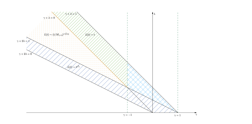
Figure 1: Dependence on time of the characteristic length as the parameters $\gamma$ and $\lambda$ change.

Comments on the critical case $\gamma+2\lambda=1$

In this paper, we also consider the limiting case $\gamma+2\lambda=1$. It appears to lead to interesting new possible asymptotic behaviour but it is also the case for which we have the least complete results. Here, we will give a few preliminary results which allow us to formulate conjectures for possible behaviour in the limiting case.

It has been observed in [4] that when $\gamma>-1$ and $\gamma+2\lambda=1$, a dimensional analysis argument implies that $M_{\gamma+\lambda}$ tends to a constant as time tends to infinity. Therefore, in this case, we do not expect the loss term of the coagulation operator to tend to infinity as time tends to infinity. Hence, we do not expect the solution $f$ to equation (1.1) to tend to zero for small sizes. Instead, we expect that in the region of small sizes the solutions to equation (1.1) behave like the solution to equation (2.6) with a constant $M_{\gamma+\lambda}$, where $M_{\gamma+\lambda}$ includes also the contribution from $f$ at large cluster sizes. We refer to [4] and to Section 2.3 for the details of the derivation of this equation. In particular, we recall that for these parameter values a self-similar solution with the standard scaling does exist, in the sense of Sec. 2.1. This self-similar solution is expected to describe the long-time behaviour, in the region of large clusters, of the solutions $f$ to equation (1.1).

Interestingly, the existence/non-existence of solutions to equation (2.6) is an open problem. In this paper, we present some formal arguments that suggest that there exists a critical value $M_{\text{crit}}$ such that when $M_{\gamma+\lambda}<M_{\text{crit}}$ a solution does not exist, while when $M_{\gamma+\lambda}\geq M_{\text{crit}}$, a solution exists. Note that this is compatible with the results in [9], where it is proven that when $\gamma+2\lambda=1$ a solution to (2.6) does not exist if $M_{\gamma+\lambda}=0$.

For the complementary case, $\gamma\leq-1$ and $\gamma+2\lambda=1$, we also conjecture that the solutions $f$ are well approximated by the solutions of (2.6) at small cluster sizes. On the other hand, for large sizes, it has been proven in [4] that there are no self-similar solutions with the additional property

$$\int_{0}^{1}x^{-\lambda}\Phi(dx)<\infty\,.$$

This result is not conclusive: there could still be standard self-similar solutions such that $\int_{0}^{1}x^{-\lambda}\Phi(dx)=\infty$. In this paper, we conjecture that, when $\gamma+2\lambda=1$ and $\gamma\leq-1$, standard self-similar solutions, for equation (2.5), with $\int_{0}^{1}x^{-\lambda}\Phi(dx)=\infty$ could exist. In Figure 6 (cf. Section 6), we emphasize that the form of the self-similar solutions strongly depends on the sign of the parameter $1-(\gamma+2\lambda)$, and it should not come as a surprise that that the analysis of the critical case $\gamma+2\lambda=1$ is highly non trivial.

2.3 Splitting the size space into inner, matching and outer regions

In this section we derive heuristically equations (2.5) and (2.6) describing, respectively, the behaviour of $f$ in the outer and the inner region. Here, we only sketch the results, as similar computations are presented in detail in [4].

As a first step, we rewrite equation (1.1) as a continuity equation for the “mass” density $xf(t,x)$. Namely, if $f$ is a solution to (1.1), then

$$\partial_{t}\left(xf(t,x)\right)+\partial_{x}J[f(t,\cdot)](x)=x\eta\left(x\right)$$ (2.8)

where the mass current observable, $J$, can be defined by

$$J[f(t,\cdot)](x):=\int_{0}^{x}dy\int_{x-y}^{\infty}dzK(y,z)yf\left(t,y\right)f\left(t,z\right).$$ (2.9)

Integrating over the $x$ variable, we get the corresponding continuity equation with source term. Assuming that the total injection rate has been scaled to one, we find

$$\partial_{t}\int_{0}^{z}xf(t,x)dx+J[f(t,\cdot)](z)=1,\qquad z>L_{\eta}\,.$$

We then split the solution $f$ into three parts, $f=f_{in}+f_{m}+f_{out}$, with $f_{in}=f_{(0,\ell)},$ $f_{m}=f_{(\ell,L_{0})}$ and $f_{out}=f_{(L_{0},\infty)}$. Here, $L_{0}:=\epsilon L(t)$ is some suitably chosen characteristic length which guarantees that most of the mass lies in $f_{out}$ (see Section 3), while $1\ll\ell\ll L_{0}(t)$. See Figure 2 for an illustration of the inner, matching and outer regions.

Using this decomposition in the definition of the flux $J$, (2.9), yields

$$J[f(t,\cdot)](z)=\int_{0}^{z}\int_{z-x}^{\infty}xK(x,y)\left[f_{in}(x)+f_{m}(x)+f_{out}(x)\right]\left[f_{in}(y)+f_{m}(y)+f_{out}(y)\right]dydx\,.$$

We can then analyse each of the resulting terms using the asymptotic behaviour of the kernel $K$, as well as using the fact that we expect a stationary solution for $x\ll L_{0}(t)$. This results in equations for $f_{in}$, $f_{m}$ and $f_{out}$.

In particular, we deduce that $f_{in}$ satisfies

$$1=J[f_{in}](z)+M_{\gamma+\lambda}\int_{0}^{z}x^{1-\lambda}f_{in}(x)dx.$$ (2.10)

Equation (2.10) is just equation (2.6) written in flux form, and we will thus assume that $\overline{f}=f_{in}$ is a solution to that equation. Since we assumed that most of the mass lies in the outer region, we can here use $M_{\gamma+\lambda}(f)=M_{\gamma+\lambda}(f_{out})$ and we will assume that $M_{\gamma+\lambda}(f_{m})\ll M_{\gamma+\lambda}(f)$. A consequence of equation (2.10) is that we expect to have that

$$M_{\gamma+\lambda}M_{1-\lambda}^{in}=1,$$ (2.11)

where we are using the notation $M_{1-\lambda}(f_{in})=M_{1-\lambda}^{in}$ and (1.10). We stress here that equation (2.10) is expected to describe the behaviour of $f$ in the inner region both when $\gamma+2\lambda>1$ (hence when $M_{\gamma+\lambda}\rightarrow\infty$ as time tends to infinity) and when $\gamma+2\lambda=1$ (hence when $M_{\gamma+\lambda}$ is constant in time). The behaviours of the solutions to (2.10) in both cases are studied in Section 4. The relation (2.11) is derived by considering $z$ going to infinity in equation (2.10).

Instead, when $z\approx\ell$, we deduce that

$$1=J[f_{m}](z)+M_{1-\lambda}^{in}z^{\gamma+\lambda+1}f_{m}(z)+M_{\gamma+\lambda}\int_{0}^{z}x^{1-\lambda}f_{m}(x)dx.$$

This equation contains the coagulation term, due to the interaction of particles of comparable sizes of order $\ell$, the loss term, due to the interaction between particles of order $\ell$ and particles of order $L$ and it contains a growth term, due to the interaction of particles of order $\ell$ with particles of order $1$. Finally, we remark that the term $1$ in the right-hand side of the above equation represents the flux of mass due to the source.

Finally, we have that $f_{out}$ satisfies

$$\partial_{t}\int_{0}^{z}xf_{out}(t,x)dx+M_{1-\lambda}^{in}z^{\gamma+\lambda+1}f(z)+J[f_{out}(t,\cdot)](z)=1\quad\text{ where }z\approx L(t).$$

Notice that (2.11) implies that this equation is just the flux formulation of equation (2.5), as expected.

Figure 2: The inner, the matching and the outer region are illustrated.

3 Characteristic length and main hypotheses when $\gamma+2\lambda>1$

In this Section, we determine the different possible qualitative behaviours for the solutions to (1.1) combining dimensional analysis arguments with some estimates for the evolution of the moments $M_{0}$ and $M_{1}$ which yield the behaviour of the total number of clusters and the total mass in the system, respectively. We start the section by recalling the dimensional analysis for the coagulation equation without source, then in Section 3.2 we will explain how these arguments change when we have the source.

The main ansatz that we make in this paper is to assume that there exists a characteristic length $L$ depending on $t$ which characterizes the typical size of the clusters for long-times. Typicality here is with respect to the probability distribution $f(t,x)/M_{0}(t)$. Since the expected value for the size of the cluster is then equal to $M_{1}/M_{0}$, our goal is to choose $L=L(t)$ so that the following relation between $[M_{1}]$ and $[M_{0}]$ is satisfied

$$\left[M_{1}\right]=\left[M_{0}\right]\left[L\right]\,,$$ (3.1)

up to some factor of order one on the right hand side. After fixing the scale $L(t)$, we also assume that it then determines the scale of all other relevant moments $q$,

$$\left[M_{q}\right]\approx\left[M_{0}\right]\left[L\right]^{q}.$$

This would certainly be true if the dominant contribution to the moment comes from a self-similar solution as in (2.2). Notice that (3.1) implicitly assumes that $M_{0}(f_{out})\approx M_{0}(f)$ and that $M_{0}(f_{in})$ is negligible. Later we will see that these assumptions are self-consistent.

3.1 Dimensional analysis without source

In this first case, we assume that there is no source and that gelation does not take place. Hence, $[M_{1}]\approx 1$. Together with (3.1) this implies that $[M_{0}]=[L]^{-1}$. On the other hand, since $f$ satisfies the coagulation equation and since the kernel is homogeneous, we have the following ODE describing the evolution in time of the $0$-th moment

$$\frac{d}{dt}M_{0}=-[M_{0}]^{2}[L]^{\gamma}.$$ (3.2)

Using the relation between $[M_{0}]$ and $L$, equation (3.2) can be rewritten as $\frac{d}{dt}[M_{0}]=-[M_{0}]^{2-\gamma}.$ Note that since $\gamma<1$, the number of particles is always decreasing in time, as expected. As we will see later this will, instead, depend on the assumptions on the parameters $\gamma$ and $\lambda$ when we consider the coagulation equation with source. Solving the ODE for $[M_{0}]$, we deduce that $[M_{0}]\approx t^{-\frac{1}{1-\gamma}}$. Hence the characteristic length is $L\approx t^{\frac{1}{1-\gamma}}$. We will next see how this argument changes if we consider the coagulation equation with a source.

3.2 Dimensional analysis with source

In this section, we will consider only the case $\gamma+2\lambda>1$ as the case $\gamma+2\lambda=1$ is different and more challenging, therefore it will be considered separately in Section 6.

Since we are in the non-gelling regime and we are considering the coagulation equation with source we deduce that the first moment evolves according to the following ODE

$$\frac{dM_{1}}{dt}=\int_{\mathbb{R}_{*}}x\eta(x)dx=1\,.$$

Here, we have adapted the microscopic time-scale so that the total injection rate from the source leads to rate one injection of the total mass. This scaling assumption will be continued to be used from now on.

In the last equality comes from our assumption that Therefore,

$$M_{1}(t)=M_{1,0}+t$$

where $M_{1,0}$ is the initial mass of monomers. We then have the following asymptotic behaviour for long-times

$$M_{1}\approx t\ \ \text{as\ \ }t\rightarrow\infty.$$ (3.3)

As in Section 3.1, the dimensional analysis, combined with our assumption on the existence of a characteristic length $L$, will allow to assume (3.1). Thanks to (3.3), this results in the following relation between $\left[M_{0}\right]$ and the characteristic length $L$

$$\left[M_{0}\right]\left[L\right]=t.$$ (3.4)

Notice that to deduce equations (3.3) and (3.4), we only used the non-gelling conditions for $\gamma$ and $\lambda$, hence these asymptotics hold for any value of $\gamma+\lambda<1$ and $\gamma<1$.

We now compute the derivative of $M_{0}.$ We use the assumption that most of the clusters are in the region where $x\gg 1$ and therefore that $M_{0}$ is given approximately by the integral (or sum) on this region of cluster sizes, i.e., $M_{0}\approx M_{0}(f_{out})$.

Using the homogeneity of the kernel, we can write the dimensions of the coagulation operator $\mathbb{K}\left[f\right]$ in (1.1) as $\left[M_{0}\right]^{2}\left[L\right]^{\gamma-1}.$ Moreover, each coagulation event reduces the number of clusters by one. On the other hand, there is an implicit source of clusters in equation (2.5), represented by the growth term. The added clusters can be transferred to large cluster sizes by means of different mechanisms which may or may not contribute to an increase of $M_{0}$.

One mechanism consists in the coagulation of a cluster with size of order one with a large cluster. However, such a transfer mechanism does not modify the number of large clusters $M_{0}.$ On the contrary the coagulation of two large clusters results in the reduction of one cluster by reaction. Therefore, the contribution of the coagulation mechanism to $\frac{dM_{0}}{dt}$ is $-\left[M_{0}\right]^{2}\left[L\right]^{\gamma},$ where we use the fact that this term yields the order of magnitude of $\int_{0}^{\infty}\mathbb{K}\left[f\right]dx.$ Finally, the number of large clusters $M_{0}$ can increase due to the flux of small clusters to large clusters, due to iterated coagulation events of the small injected clusters. The flux of clusters from small cluster to large cluster sizes has been computed in (2.7).

We then have the following equation that yields the order of magnitude for the change of $M_{0}$

$$\frac{dM_{0}}{dt}=J_{c}\left(M_{\gamma+\lambda}\right)-\left[M_{0}\right]^{2}\left[L\right]^{\gamma},$$

We notice that this equation can be obtained from (2.5) by integrating over the size variable and taking into account the influx of particles from zero, represented here by $J_{c}(M_{\gamma+\lambda})$. Combining the previous formula with (3.4) we obtain the following equation for $M_{0}$

$$\frac{dM_{0}}{dt}=J_{c}\left(M_{\gamma+\lambda}\right)-\left[M_{0}\right]^{2-\gamma}t^{\gamma}.$$ (3.5)

The equation (3.5) allows to obtain many different behaviours for the solutions for different choices of the exponents $\gamma$ and $\lambda.$ Let us point out that the type of behaviours allowed by (3.5) is much richer than the ones obtained for the coagulation equation without injection (3.2). A major difference with the problem without injection is the fact that in the problem with injection we can have both increasing and decreasing number of clusters $M_{0}.$ In the case of coagulation without injection the number of clusters $M_{0}$ can only decrease due to the effect of the coagulation.

By (2.7), the fluxes $J_{c}\left(M_{\gamma+\lambda}\right)$ depend exponentially in $M_{\gamma+\lambda}$. Our assumption about the characteristic length $L$ indicates that $\left[M_{\gamma+\lambda}\right]=\left[M_{0}\right]\left[L\right]^{\gamma+\lambda}.$ Now if $M_{\gamma+\lambda}$ tends to infinity as a power law of $t$, the flux of monomers $J_{c}\left(M_{\gamma+\lambda}\right)$ would be exponentially small and therefore the gain of monomers would be negligible. In such a case, the number of clusters evolves according to the equation

$$\frac{dM_{0}}{dt}=-\left[M_{0}\right]^{2-\gamma}t^{\gamma}$$ (3.6)

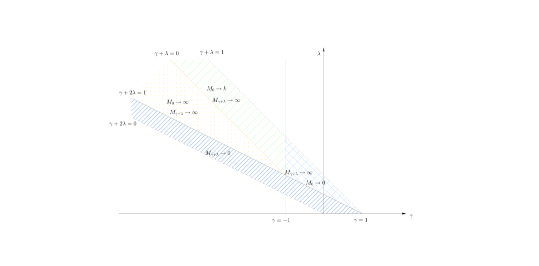
Figure 3: In this picture we show how the behaviour of the moments $M_{\gamma+\lambda}$ and $M_{0}$ change as the parameters $\lambda$ and $\gamma$ change.

We stress that the approximation (3.6) can be expected to be valid only if $M_{\gamma+\lambda}$ tends to infinity sufficiently fast, for instance, like a power law. Failing that, the analysis of (3.5) suggests different behaviours for $M_{0}$. We refer to Figure 3 for a summary of how $M_{0}$ and $M_{\gamma+\lambda}$ change depending on the parameters $\gamma$ and $\lambda$. The results from the analysis of the various scenarios in the regime $\gamma+2\lambda>1$ are summarized in the following:

• If $\gamma>-1$, we obtain from (3.6) the asymptotics $\left[M_{0}\right]\approx t^{-\frac{1+\gamma}{1-\gamma}}.$ Then, the number of clusters converges to zero and (3.4) implies $L\approx t^{\frac{2}{1-\gamma}}.$ This corresponds to the self similar behaviour that has been considered in [4], see equality (2.2) for the self-similar solution. Note that in this case we have $\left[M_{\gamma+\lambda}\right]=\left[M_{0}\right]\left[L\right]^{\gamma+\lambda}\approx t^{\frac{\gamma+2\lambda-1}{1-\gamma}}$ that converges to infinity as a power law, since $\gamma+2\lambda>1$. This implies that $J_{c}\left(M_{\gamma+\lambda}\right)$ converges to zero exponentially fast, justifying the approximation (3.6) and therefore asserting the self-consistency of this approximated equation.

• If $\gamma=-1$, we obtain the asymptotic behaviour $\left[M_{0}\right]\approx\left(\log\left(t\right)\right)^{-\frac{1}{2}}.$ Using (3.4) we obtain $L\approx t\left(\log\left(t\right)\right)^{\frac{1}{2}}$ as $t\rightarrow\infty.$ This corresponds to a class of self-similar solutions with a logarithmic correction that will be described in Section 5.3. Note that in this case we have

  $$\left[M_{\gamma+\lambda}\right]\approx\left(\log\left(t\right)\right)^{\frac{1}{2}\left(\gamma+\lambda-1\right)}t^{\gamma+\lambda}=\left(\log\left(t\right)\right)^{\frac{1}{2}\left(\lambda-2\right)}t^{\lambda-1}\text{ as }t\rightarrow\infty.$$

  Since $\gamma+2\lambda>1$ and $\gamma=-1$, we have here $\lambda>1.$ Hence, $\left[M_{\gamma+\lambda}\right]$ tends to infinity like a power law. Therefore, given (2.7), $J_{c}\left(M_{\gamma+\lambda}\right)$ is exponentially small, showing the consistency of the approximation (3.6).

• If $\gamma<-1$ we have two possibilities:

  • If $\left(\gamma+\lambda\right)>0$, (3.6) implies that $M_{0}$ approaches to a constant as $t\rightarrow\infty.$ We expect the number of clusters to tend to a constant for large times, because the rate of destruction of clusters due to the coagulation process is too slow to make the number of cluster decreasing and the flux of particles from the origin is too slow to make it increase. Using (3.4) it follows that $L\approx t.$ Then $\left[M_{\gamma+\lambda}\right]\approx t^{\gamma+\lambda}.$ Therefore, if $\left(\gamma+\lambda\right)>0$, we obtain that the fluxes $J_{c}\left(M_{\gamma+\lambda}\right)$ are exponentially small and the approximation (3.6) is self-consistent.

  • If $\left(\gamma+\lambda\right)\leq 0$, dimensional considerations do not imply $\left[M_{\gamma+\lambda}\right]$ approaching polynomially to infinity for large times. Therefore, due to (2.7) we can expect to have a nontrivial contribution to the number of clusters $M_{0}$ due to the fluxes of small clusters to large clusters $J_{c}\left(M_{\gamma+\lambda}\right)$. Due to the exponential dependence of the fluxes $J_{c}\left(M_{\gamma+\lambda}\right)$ in $M_{\gamma+\lambda}$, the only way in which we can avoid these fluxes to be exponentially small is by assuming that they increase at most in a logarithmic manner in $t$ (by construction with a power law behaviour) as $t\rightarrow\infty.$ Using that $\left[M_{\gamma+\lambda}\right]=\left[M_{0}\right]\left[L\right]^{\gamma+\lambda}$ and using also (3.4) it follows that

    $$L^{1-\left(\gamma+\lambda\right)}\approx\frac{t}{[M_{\gamma+\lambda}]}.$$ (3.7)

    Then $[M_{0}]\cdot t^{\frac{\left(\gamma+\lambda\right)}{1-\left(\gamma+\lambda\right)}}\approx[M_{\gamma+\lambda}]^{\frac{1}{1-(\gamma+\lambda)}}.$ Therefore, the contribution of the coagulation term to $-\frac{dM_{0}}{dt}$ is of the order $\left[M_{0}\right]^{2-\gamma}t^{\gamma}\approx\frac{\left[M_{0}\right][M_{\gamma+\lambda}]^{\frac{1-\gamma}{1-(\gamma+\lambda)}}}{t^{\frac{\lambda}{1-\left(\gamma+\lambda\right)}}}.$ Since $M_{\gamma+\lambda}$ grows logarithmically, we have that, when $\gamma+2\lambda>1$, it then follows that this term is much smaller than $\frac{dM_{0}}{dt}.$ Therefore (3.5) reduces to

    $$\frac{dM_{0}}{dt}=J_{c}\left(M_{\gamma+\lambda}\right).$$

    Using now (2.7) we can obtain the logarithmic dependence of $M_{\gamma+\lambda}.$ Indeed, using that $[M_{0}]\approx[M_{\gamma+\lambda}]^{\frac{1}{1-(\gamma+\lambda)}}\cdot t^{-\frac{\left(\gamma+\lambda\right)}{1-\left(\gamma+\lambda\right)}}$ it then follows that

    $$M_{\gamma+\lambda}\simeq\left(\frac{1}{a_{\gamma+2\lambda}}\log\left(t^{\frac{1}{1-\left(\gamma+\lambda\right)}}\right)\right)^{\frac{\gamma+2\lambda}{2}}\ \ \text{as\ \ }t\rightarrow\infty.$$ (3.8)

    We stress that the constant $a_{\gamma+2\lambda}$ in (3.8) depends on the value of $\gamma+2\lambda$.

    Combining this formula with $\left[M_{\gamma+\lambda}\right]=\left[M_{0}\right]\left[L\right]^{\gamma+\lambda}$ and (3.4) we can obtain the scaling laws for $M_{0}$ and $L$ (including logarithmic terms). These scalings will allow to obtain approximate solutions to the coagulation equation, that will be determined in Section 5.2.

The dimensional considerations above include all the cases for which standard self-similar solutions to equation (1.1) do not exist for homogeneous kernels of the form (1.7) with $F$ satisfying (1.8) and the non-gelation conditions (1.9). In the following sections we provide the formal computations, based on asymptotic analysis techniques, that allow to justify the long-time behaviour of the solutions to (1.1).

4 Behaviour in the inner region

In this section we analyse the long-time behaviour of the solutions $f$ to equation (1.1) in the region of sizes $x$ of order $1$. We assume that the kernel $K$ satisfies (1.7) and (1.8) with parameters that satisfy the non-gelation condition (1.9) and that satisfy $\gamma+2\lambda\geq 1$.

As already anticipated in the introduction, we expect two different behaviours depending on the long-time behaviour of the $M_{\gamma+\lambda}$ moment. As we discussed in Section 3, dimensional considerations imply that when $\gamma+2\lambda>1$, then $M_{\gamma+\lambda}$ tends to infinity as time tends to infinity (although in different ways depending on the signs of $\gamma+1$ and of $\gamma+\lambda$). The long-time behaviour of the solution $f$ to equation (1.1) in the region of small sizes corresponding to $M_{\gamma+\lambda}\rightarrow\infty$ as $t\rightarrow\infty$ is studied in Section 4.1.

When, instead, $\gamma+2\lambda=1$ and $\gamma>-1$, dimensional considerations show that $M_{\gamma+\lambda}$ tends to a constant as time goes to infinity. For more details, we refer to [4] and to Section 3. When $\gamma+2\lambda=1$ and $\gamma\leq-1$, we also expect that $M_{\gamma+\lambda}$ tends to a constant and therefore we expect the same behaviour as in the case $\gamma+2\lambda=1$ and $\gamma>-1$ in the inner region. For this set of parameters, the long-time behaviour of the solution $f$ to equation (1.1) in the region of small sizes is studied in Section 4.2.

4.1 Behaviour of the solutions to (2.6) when $M_{\gamma+\lambda}\rightarrow\infty$ as $t\rightarrow\infty$

The goal of this Section is to obtain the behaviour of the solutions to (2.6) when the moment $M_{\gamma+\lambda}\to\infty$ for large times. In order to do this, we first recall that there exists a characteristic cluster size $L\left(t\right)$ satisfying $\lim_{t\rightarrow\infty}L\left(t\right)=\infty$ such that most of the monomers of the system are contained in the clusters with sizes of order $L\left(t\right).$

We make some additional assumption which will allow to simplify the problem.

• The cluster distribution $f(t,x)$ can be approximated by means of a discrete distribution $c_{n}(t)$ for small values of $x.$

• We will assume that $\eta_{n}=a\delta_{n,1}$ for some $a>0.$ Rescaling the values of $c_{n}$ and changing the unit of time we can assume without loss of generality that $a=1.$

Combining the assumption on the existence of a characteristic size with the approximation $K\left(j,n\right)\simeq\left(j\right)^{\gamma+\lambda}\left(n\right)^{-\lambda}$ for $n$ of order one and $j$ large, as well as, assumptions (i) and (ii) we obtain the following discrete version of equation (2.6) for the concentrations $c_{n}\left(t\right)$ in the inner region, namely when $n\approx 1$,

$$\frac{1}{2}\sum_{j=1}^{n-1}K\left(n-j,j\right)c_{n-j}c_{j}-\left[\sum_{j=1}^{L\left(t\right)}K\left(j,n\right)c_{j}\right]c_{n}-\frac{M_{\gamma+\lambda}}{\left(n\right)^{\lambda}}c_{n}+\delta_{n,1}=0.$$ (4.1)

We mention that a similar strategy has been used for a Becker–Döring model in [14].

We make also the following additional assumption which allows to simplify (4.1).

• We consider only solutions to (4.1) that satisfy

  $$\sum_{j=2}^{L\left(t\right)}K\left(j,n\right)c_{j}\ll\max\left\{K\left(1,n\right)c_{1},\frac{M_{\gamma+\lambda}}{\left(n\right)^{\lambda}}\right\}$$ (4.2)

  as $M_{\gamma+\lambda}\rightarrow\infty$ uniformly for all the values of $n\in\left[1,L\left(t\right)\right].$

We notice that condition (iii) is motivated by the strong interaction between particles of size $1$ and $n$ that, as explained in the introduction, we expect to have when $\gamma+2\lambda\geq 1$. Assumption (iii) implies that we can approximate (4.1) by

$$\frac{1}{2}\sum_{j=1}^{n-1}K\left(n-j,j\right)c_{n-j}c_{j}-K\left(1,n\right)c_{1}c_{n}-\frac{M_{\gamma+\lambda}}{\left(n\right)^{\lambda}}c_{n}+\delta_{n,1}=0.$$ (4.3)

Notice that the equation (4.3) can be solved recursively for arbitrary values of $n.$ Indeed, we can determine $c_{1}$ as the unique positive solution to the equation

$$K\left(1,1\right)\left(c_{1}\right)^{2}+M_{\gamma+\lambda}c_{1}=1$$ (4.4)

Therefore, we can determine $c_{n}$ for $n\geq 2$ by means of the iterative formula

$$c_{n}=\frac{1}{2\left(K\left(1,n\right)c_{1}+\frac{M_{\gamma+\lambda}}{\left(n\right)^{\lambda}}\right)}\sum_{j=1}^{n-1}K\left(n-j,j\right)c_{n-j}c_{j}\ \ \ \ n\geq 2.$$ (4.5)

It is then possible to prove that the solutions to (4.4), (4.5) satisfy the following asymptotics

$$c_{n}\simeq\frac{\left[\left(2\pi\right)^{\frac{\gamma}{2}+\lambda}K\right]\left(M_{\gamma+\lambda}\right)^{2}}{n^{\gamma+\lambda}\sqrt{1+\frac{\left(M_{\gamma+\lambda}\right)^{2}}{n^{\gamma+2\lambda}}}}\exp\left(-\left(M_{\gamma+\lambda}\right)^{\frac{2}{\gamma+2\lambda}}\int_{0}^{\frac{n}{\left(M_{\gamma+\lambda}\right)^{\frac{2}{\gamma+2\lambda}}}}\log\left(1+\frac{1}{y^{\gamma+2\lambda}}\right)dy\right)$$ (4.6)

as $M_{\gamma+\lambda}\rightarrow\infty$ and $1\ll n\ll L\left(t\right)$ for a suitable constant $K>0$ independent of $M_{\gamma+\lambda}.$

Strategy for the justification of (4.6)

In this section we only give the main ideas for the computation of (4.6), some more details can be found in the appendix A. These ideas are very similar to the ones in [12], [13]. First of all notice that, if $M_{\gamma+\lambda}\rightarrow\infty$, we can approximate the first values of the sequence $\left\{c_{n}\right\}_{n\in\mathbb{N}}$ solving (4.4), (4.5). We have

$$c_{1}\simeq\frac{1}{M_{\gamma+\lambda}}\ ,\ \ c_{2}\simeq\frac{1}{2}\frac{2^{\lambda}K\left(1,1\right)}{\left(M_{\gamma+\lambda}\right)^{3}}\ ,\ \ c_{3}\simeq\frac{1}{2}\frac{3^{\lambda}2^{\lambda}K\left(2,1\right)\left(K\left(1,1\right)\right)^{2}}{\left(M_{\gamma+\lambda}\right)^{5}}\ ,\ ...$$ (4.7)

We now want to approximate the values of $\left\{c_{n}\right\}_{n\in\mathbb{N}}$ using the approximation given by (4.5) for a range of values of $n$ for which the term $K\left(1,n\right)\left(n\right)^{\lambda}c_{1}$ becomes comparable or larger than $M_{\gamma+\lambda}.$ Notice that, due to the asymptotics of $c_{1}$ in (4.7) we have that $K\left(1,n\right)\left(n\right)^{\lambda}c_{1}$ becomes comparable to $M_{\gamma+\lambda}$ if $K\left(1,n\right)\left(n\right)^{\lambda}c_{1}\simeq\frac{\left(n\right)^{\gamma+2\lambda}}{M_{\gamma+\lambda}}\approx M_{\gamma+\lambda},$ i.e., for  $n\approx\left(M_{\gamma+\lambda}\right)^{\frac{2}{\gamma+2\lambda}}.$

We would like to check that the main contribution to the convolution term $\sum_{j=1}^{n-1}K\left(n-j,j\right)c_{n-j}c_{j}$ is due to the terms multiplying $c_{1}$ if $t\rightarrow\infty$ and $1\ll n\leq L\left(t\right).$ We first check this for the range of values of $n$ for which $K\left(1,n\right)\left(n\right)^{\lambda}c_{1}\ll M_{\gamma+\lambda},$ i.e., $n\ll\left(M_{\gamma+\lambda}\right)^{\frac{2}{\gamma+2\lambda}}.$ In this case, we can approximate (4.5) as

$$c_{n}=\frac{\left(n\right)^{\lambda}}{M_{\gamma+\lambda}}\left[\frac{1}{2}\sum_{j=1}^{n-1}K\left(n-j,j\right)c_{n-j}c_{j}+\delta_{n,1}\right]\ \ ,\ \ n\geq 1.$$ (4.8)

The asymptotic formulas (4.7) suggest to rescale the concentrations $c_{n}$ as

$$c_{n}=\frac{X_{n}}{\left(M_{\gamma+\lambda}\right)^{2n-1}}\ \ ,\ \ n\in\mathbb{N}.$$ (4.9)

Using (4.8) then we obtain the following equation for the variables $X_{n}$

$$X_{n}=\frac{\left(n\right)^{\lambda}}{2}\sum_{j=1}^{n-1}K\left(n-j,j\right)X_{n-j}X_{j}\ \ ,\ \ n\geq 2\ \ ,\ \ X_{1}=1.$$ (4.10)

Notice that (4.10) allows to obtain the sequence of coefficients $\left\{X_{n}\right\}_{n\in\mathbb{N}}$ in an iterative manner. We claim that under the assumption $\gamma+2\lambda\geq 1$ the asymptotic behaviour of the solutions to (4.10) can be approximated by the solutions to the problem

$$X_{n}=\left(n\right)^{\lambda}K\left(n-1,1\right)X_{n-1}X_{1}\ \ \ \text{for }n\text{ large}.$$ (4.11)

Using (1.7), (1.8), as well as the fact that $X_{1}=1$, we obtain the leading order approximation

$$X_{n}=\left(n\right)^{\gamma+2\lambda}X_{n-1}\ \ \text{for }n\text{ large}$$

and, finally we deduce the approximation

$$X_{n}\simeq\frac{K}{n^{\gamma+\lambda}}\left(n!\right)^{\gamma+2\lambda}\ \ \text{as }n\rightarrow\infty$$ (4.12)

for some suitable constant $K$.

Some careful computations combined with the use of Euler–Maclaurin formulas as well as Stirling’s approximation for the factorial in (4.12) then lead to desired asymptotics for the concentrations $c_{n}$ (cf.(4.6)). We refer to the appendix A for further details.

4.2 Solutions to (2.6) for $M_{\gamma+\lambda}$ of order $1$

In this section, we discuss formal asymptotics on the behaviour of the solutions to equation (2.6). In particular, assuming that a solution to (2.6) exists, we derive the following large-size behaviour for the solution $\overline{f}$ to equation (2.6)

$$\overline{f}(x)\approx x^{\lambda-1}x^{-M_{\gamma+\lambda}^{2}}\text{ as }x\rightarrow\infty$$ (4.13)

when $M_{\gamma+\lambda}\neq 1$ and

$$\overline{f}(x)\approx\frac{1}{x^{(\gamma+3)/2}(\ln(x))^{2}}\text{ as }x\rightarrow\infty$$ (4.14)

when $M_{\gamma+\lambda}=1$.

Notice that, when $M_{\gamma+\lambda}<1$ the assumption that a solution $\overline{f}$ of (2.6) exists together with (4.13), implies that

$$\int_{0}^{\infty}x^{1-\lambda}\overline{f}(x)dx=\infty.$$

This is a contradiction. Indeed a solution to equation (2.6) should be such that $M_{1-\lambda}(\overline{f})\leq 1/M_{\gamma+\lambda}<\infty$ as will be explained in Step 1. This is the reason why we expect solutions to equation (2.6) to exist only when $M_{\gamma+\lambda}>1$.

Before showing how we obtain the asymptotics (4.13) and (4.14) we stress that the behaviour for $\overline{f}$ in (4.14) reminds the one derived in [9] for $M_{\gamma+\lambda}=0$ and for $\gamma+2\lambda<1$, i.e., $\overline{f}\approx x^{-(\gamma+3)/2}$ for $x$ large, but here we have logarithmic corrections.

The rest of the section is devoted to the derivation of (4.13) under the assumption that $M_{\gamma+\lambda}\neq 1$. We do not show (4.14) as it can be proven using very similar arguments. We present here preliminary results: a detailed and rigorous analysis of the existence of solutions for equation (2.6) is challenging and goes beyond the aim of this paper.

We divide the derivation of (4.13) in steps as follows.

Step 1: Reformulation of equation (2.6)

As a first step to derive (4.13), it is convenient to rewrite equation (2.6) in flux form as follows:

$$J[\overline{f}](x)=\int_{0}^{x}z\eta(z)dz-M_{\gamma+\lambda}\int_{0}^{x}z^{1-\lambda}\overline{f}(z)dz.$$ (4.15)

Here $J[\overline{f}](x)$ is the flux of mass from the region of particles of size less than $x$ to the region of particles of sizes bigger than $x$ and is defined as in (2.9), namely

$$J[\overline{f}](x)=\int_{0}^{x}\int_{x-z}^{\infty}K(y,z)z\overline{f}(z)\overline{f}(y)dydz.$$

Motivated by (4.15), we define the function $g$ as $g(x):=x^{1-\lambda}\overline{f}(x)$. Then $g$ satisfies the following equation

$$\tilde{J}[g](x)=\int_{0}^{x}z\eta(z)dz-M_{\gamma+\lambda}\int_{0}^{x}g(z)dz$$ (4.16)

where

$$\tilde{J}[g](x):=\int_{0}^{x}\int_{x-z}^{\infty}W(y,z)g(z)g(y)dydz=J[\overline{f}](x)\quad\text{ with }\quad W(y,z)=z^{\lambda}y^{\lambda-1}K(y,z).$$

We now study the behaviour of the solution $g$ to equation (4.16) as $x\rightarrow\infty$.

To this end we first show that

$$\int_{0}^{\infty}z\eta(z)dz=M_{\gamma+\lambda}\int_{0}^{\infty}g(z)dz.$$ (4.17)

Step 2: (4.17) holds

Since $g$ is a solution to equation (4.16), then $\int_{0}^{\infty}g(x)dx\leq\frac{1}{M_{\gamma+\lambda}}.$ Assume, by contradiction, that $\int_{0}^{\infty}z\eta(z)dz\neq M_{\gamma+\lambda}\int_{0}^{\infty}g(z)dz$. This would imply that there exists a constant $c>0$ such that

$$\int_{0}^{\infty}z\eta(z)dz-M_{\gamma+\lambda}\int_{0}^{\infty}g(z)dz=c=\lim_{x\rightarrow\infty}\tilde{J}[g](x).$$

Since in [9] it has been proven that the equation for the constant flux solution $J[f]=c$ does not have solutions when $\gamma+2\lambda\geq 1$, we deduce that $c=0.$ Therefore, (4.17) follows.

Step 3: equation for $\int_{x}^{\infty}g(y)dy$

As a consequence of Step 2, considering large values of $x$ in equation (4.16), we have that

$$\tilde{J}[g](x)=M_{\gamma+\lambda}\int_{x}^{\infty}g(z)dz.$$ (4.18)

We introduce the notation $G(x):=\int_{x}^{\infty}g(y)dy$. Thanks to Step 2 we know that $G(x)\rightarrow 0$ as $x\rightarrow\infty$. Moreover (4.17) implies that

$$G(x)\int_{0}^{x}g(z)dz=\frac{1}{M_{\gamma+\lambda}}G(x)-G(x)^{2}$$

where we normalized the source $\eta$ so that $\int_{0}^{\infty}x\eta(x)dx=1$.

The above observation allows to rewrite equation (4.18) as

$$\int_{0}^{x}g(z)\int_{x}^{\infty}\left[W(y,z)-1\right]g(y)dydz+\int_{0}^{x}g(z)\int_{x-z}^{x}W(y,z)g(y)dydz=\left(M_{\gamma+\lambda}-\frac{1}{M_{\gamma+\lambda}}\right)G(x)+G(x)^{2}.$$ (4.19)

We recall that, since the source is zero in $(0,1]$, then $\overline{f}((0,1))=0$ and $g((0,1))=0$.

Step 4: the first term in left-hand side of (4.19) tends to zero faster than $G(x)$ as $x\rightarrow\infty$

Let us consider a function $\varepsilon(x)$ such that $\varepsilon=\varepsilon(x)\rightarrow 0$ as $x\rightarrow\infty$ so slowly that $G(\varepsilon(x)x)\rightarrow 0$ as $x\rightarrow\infty$. We can rewrite the first term on the left hand side of equation (4.19) as follows

$$\int_{0}^{x}g(z)\int_{x}^{\infty}\left[W(y,z)-1\right]g(y)dydz=\int_{1}^{\varepsilon x}g(z)\int_{x}^{\infty}\left[W(y,z)-1\right]g(y)dydz$$

$$+\int_{\varepsilon x}^{x}g(z)\int_{x}^{\infty}\left[W(y,z)-1\right]g(y)dydz.$$

Using the fact that on the domain of integration of the first integral on the right-hand side of the equality above we have that $z\ll y$, we can use the approximation for $K$ given by (1.8), together with the fact that $\gamma+2\lambda=1$, to deduce that for large values of $x$

$$\int_{1}^{\varepsilon x}g(z)\int_{x}^{\infty}\left[W(y,z)-1\right]g(y)dydz\leq\varepsilon G(1)G(x)$$

where $\varepsilon=\varepsilon(x)$ tends to zero as $x\rightarrow\infty$.

On the other side, using again the properties of the kernel $W$ we deduce that

$$\int_{\varepsilon x}^{x}g(z)\int_{x}^{\infty}\left[W(y,z)-1\right]g(y)dydz\leq G(\varepsilon x)G(x).$$

The desired conclusion then follows.

Step 5: approximation of the second term in left-hand side of (4.19) as $x\rightarrow\infty$

We rewrite the second term in the left-hand side of equation (4.19) as follows

$$\iint_{S_{x}}W(y,z)g(y)g(z)dydz=\iint_{S_{x}\cap\{y<\varepsilon z\}}W(y,z)g(y)g(z)dydz+\iint_{S_{x}\cap\{\varepsilon z<y<\frac{z}{\varepsilon}\}}W(y,z)g(y)g(z)dydz$$

$$+\iint_{S_{x}\cap\{y>\frac{z}{\varepsilon}\}}W(y,z)g(y)g(z)dydz$$

where $S_{x}:=\{(y,z)\in\mathbb{R}_{*}\times\mathbb{R}_{*}:0<z<x,\ x-z<y<x\}$.

Now notice that

$$\iint_{S_{x}\cap\{\varepsilon z<y<\frac{z}{\varepsilon}\}}W(y,z)g(y)g(z)dydz\leq(G(\varepsilon x))^{2}.$$

On the other side, using the asymptotics of the kernel $W$, we deduce that, as $x\rightarrow\infty$

$$\iint_{S_{x}\cap\{y<\varepsilon z\}}W(y,z)g(y)g(z)dydz+\iint_{S_{x}\cap\{y>\frac{z}{\varepsilon}\}}W(y,z)g(y)g(z)dydz$$

$$\approx\int_{1}^{\varepsilon x}\int_{x-z}^{x}\left(1+\frac{y}{z}\right)g(y)g(z)dydz\approx x\int_{1}^{\varepsilon x}\frac{G(x-z)-G(x)}{z}g(z)dz\approx-xG(1)\frac{dG(x)}{dx}.$$

Step 6: asymptotics of $f$

Using the asymptotics computed in Steps 4 and 5 as well as the fact that $M_{\gamma+\lambda}>1$ and keeping only the leading terms in (4.19), we deduce

$$-xG(1)\frac{dG(x)}{dx}\approx\left(M_{\gamma+\lambda}-\frac{1}{M_{\gamma+\lambda}}\right)G(x)$$

as $x$ tends to infinity. Therefore, for large sizes $x$ we expect that

$$G(x)\approx x^{-(M_{\gamma+\lambda}^{2}-1)},$$

where we used (2.11) since $G(1)=M^{in}_{1-\lambda}$. From this we infer that, for large sizes, $g(x)\approx x^{-M_{\gamma+\lambda}^{2}}$ and, therefore, (4.13) follows.

5 Anomalous self-similarity for $\gamma+2\lambda>1$

In this section we study the anomalous self-similar solutions to equation (2.5) under the assumptions that $\gamma+2\lambda>1$ and $\gamma\leq-1$. Notice that in all the cases specified below we expect that these self-similar solutions describe the long-time behaviour of equation (1.1). The self-similar behaviour need to be matched with (2.7) in the region of small sizes.

We divide this section according to different assumptions on the parameters $\gamma$ and $\lambda$ that lead to different scalings. We start briefly recalling the dimensional analysis in Section 3 and summarizing the self-similar behaviour derived in this section, in the regime $\gamma+2\lambda>1$, $\gamma\leq-1$.

• If $\gamma<-1$ and $\gamma+\lambda>0$, the dimensional analysis in Section 3 implies that $M_{0}$ approaches to a constant as $t\rightarrow\infty$. This is due to the fact that the rate of destruction of clusters due to the coagulation process is slow and at the same time the influx of small particles is negligible, more precisely since $\left[M_{\gamma+\lambda}\right]\approx t^{\gamma+\lambda}$ then $J_{c}\left(M_{\gamma+\lambda}\right)$ is exponentially small. The scaling is

  $$L(t)=t.$$

  The self-similar solution is of the form given by a Dirac $\delta$-function,

  $$f(t,x)=\frac{b}{t}\delta\left(\frac{x}{t}-\frac{1}{b}\right).$$

  Here, the constant $b$ depends on the initial data.

• If $\gamma<-1$, and $\gamma+\lambda\leq 0$, the dimensional analysis made in Section 3 suggests that $M_{0}$ tends to infinity as time tends to infinity. This is due to the influx of small particles in the system which, in this case, is stronger than the coagulation term. For these reasons, we expect the moment $M_{\gamma+\lambda}$ to increase at most logarithmically in time so that $J_{c}(M_{\gamma+\lambda})$ is not negligible. The scaling is

  $$L(t)=\left(\frac{t}{M_{\gamma+\lambda}}\right)^{\frac{1}{1-\gamma-\lambda}}.$$

  The corresponding self-similar solution will be

  $$f(t,x)=\frac{t}{\left(\frac{t}{M_{\gamma+\lambda}}\right)^{\frac{2}{1-(\gamma+\lambda)}}}\Phi_{\infty}\left(\frac{x}{\left(\frac{t}{M_{\gamma+\lambda}}\right)^{\frac{1}{1-(\gamma+\lambda)}}}\right)$$

  where $\Phi_{\infty}$ is given by

  $$\Phi_{\infty}(\xi)=\frac{C}{\xi^{\gamma+\lambda}}\exp\left(\int_{0}^{\xi}\frac{1}{\left(1-(\gamma+\lambda)-\eta^{1-(\gamma+\lambda)}\right)}\frac{d\eta}{\eta^{\gamma+\lambda}}\right).$$

• If $\gamma=-1$ (hence $\gamma+\lambda>0$), the dimensional analysis made in Section 3 suggests that $M_{0}$ tends to zero as time goes to infinity. This is due to the fact that the contribution to the evolution of the number of particles of the coagulation operator is larger than the influx of particles $[J_{c}(M_{\gamma+\lambda})]$. Indeed, in this case we have that $M_{\gamma+\lambda}\sim t^{\lambda-1}(\log(t))^{1/2(\lambda-2)}$, hence, $M_{\gamma+\lambda}$ increases like a power law. The contribution due to the injected small particles to the total number of particles, $J_{c}(M_{\gamma+\lambda})$, is therefore negligible. The characteristic length is

  $$L(t)=t(\ln(t))^{1/2}.$$

  The corresponding self-similar solution is

  $$f(t,x)=\frac{1}{at\ln(t)}\delta\left(\frac{x}{t\ln(t)^{1/2}}-a\right).$$

  Here the constant $a$ depends on the kernel, i.e., $a^{2}=K(1,1)$.

5.1 Self-similarity when $\gamma+\lambda>0$, $\gamma<-1$

In Section 3 we showed that when $\gamma+\lambda>0$, $\gamma<-1$ and $\gamma+2\lambda>1$, equation (1.1) is compatible with a self-similar behaviour. In particular, we expect the solutions $f$ to equation (1.1) to behave, as time goes to infinity and in the region of large sizes, as self-similar solutions to equation (2.5) with the following scaling properties:

$$[x]=\left[t\right]\quad\text{ and }\quad[f]=\frac{1}{[t]}.$$ (5.1)

The aim of this Section is to study these self-similar solutions and check that they are consistent with the scenario derived in Section 3.

Time dependent equation in self-similar variables

Motivated by (5.1), we consider the change of variables

$$f(t,x)=\frac{1}{t}\Phi(\tau,y)\quad\text{ with }\ \tau=\ln(t)\ \text{ and }\ y=\frac{x}{t}$$

in equation (2.5) and deduce that the function $\Phi$ should satisfy the following equation

$$\partial_{\tau}\Phi(\tau,y)-\Phi(\tau,y)-y\partial_{y}\Phi(\tau,y)+\frac{\partial_{y}(y^{\gamma+\lambda}\Phi(\tau,y))}{\int_{\mathbb{R}_{*}}x^{\gamma+\lambda}\Phi(\tau,x)dx}=e^{(1+\gamma)\tau}\mathbb{K}[\Phi](\tau,y)$$ (5.2)

We recall from the dimensional analysis of Section 3 that the moment $M_{0}[\Phi](\tau)$ converges to a constant as time goes to infinity. We will denote this constant by $M_{0,\infty}:=\lim_{\tau\to\infty}M_{0}[\Phi](\tau)$.

Since we are assuming that $1+\gamma<0$, the coagulation term in the above equation becomes negligible as $\tau$ tends to infinity. Hence, the above equation can be approximated by the following equation, for large $\tau$,

$$\partial_{\tau}\Phi(\tau,y)+\partial_{y}\left(\left(\frac{y^{\gamma+\lambda}}{M_{\gamma+\lambda}}-y\right)\Phi(\tau,y)\right)=0.$$ (5.3)

We make the ansatz that $\Phi(\tau,\cdot)\to\Phi_{b}$ as $\tau\to\infty$, where $\Phi_{b}$ is a solution to

$$\frac{d}{dy}\left(\left(\frac{y^{\gamma+\lambda}}{M_{\gamma+\lambda}}-y\right)\Phi(y)\right)=0$$ (5.4)

We will see in the rest of this subsection that this ansatz is self-consistent.

The self-similar profile

As explained in more detail below, (5.4) has a family of solutions $\Phi_{b}$ given by

$$\Phi_{b}(y)=b\,\delta\left(y-\frac{1}{b}\right),\quad b>0.$$ (5.5)

To compute the value of $b$, we impose that $\int_{0}^{\infty}\Phi_{b}(y)dy=M_{0,\infty}.$ Hence,

$$b=M_{0,\infty}.$$ (5.6)

We note that the value of $b$ depends on the initial value $\Phi(y,0)$ because $M_{0}$ is not constant under the evolution (5.3). Actually, $M_{0}$ is modified significantly for times $\tau$ of order $1$ by the coagulation term on the right hand-side of (5.2) in a way which strongly depends on the initial data. On the other hand, we will check next that $\Phi(y,\tau)$ can approach $\Phi_{b}(y)$ in (5.5), with $b>0$ arbitrary. We stress that this is very different from the situation that takes place in the critical case $\gamma=-1,\gamma+2\lambda>1$ (see Section 5.3). For this critical case, a suitable function $\Phi(y,\tau)$ approaches to $b\delta(y-\frac{1}{b})$ as $\tau\to\infty$, but the value of $b$ is uniquely determined by the collision kernel $K$ independently of the initial data.

Convergence to the self-similar profile

We will now show that the steady states $\Phi_{b}$ defined in (5.5) are asymptotically stable as $\tau\to\infty$ by using the method of characteristics to solve (5.3).

We start by applying a change of variables to obtain a simpler form of the model. We define the new variables

$$G(w,s)=y^{\gamma+\lambda}\Phi(y,\tau),\quad kw=\frac{y^{1-(\gamma+\lambda)}}{1-(\gamma+\lambda)},\quad s=(1-(\gamma+\lambda))\tau,$$

where the constant $k$ is defined by

$$\frac{k^{a}}{(1-(\gamma+\lambda))^{\frac{1}{1-(\gamma+\lambda)}}}=1,\quad\text{ with }\quad a:=\frac{\gamma+\lambda}{1-(\gamma+\lambda)}.$$

Then, (5.3) becomes

$$\frac{\partial G}{\partial s}+\frac{\partial}{\partial w}\left(\left(\frac{1}{\int_{0}^{\infty}G(\eta,s)\eta^{a}d\eta}-w\right)G\right)=0,\quad w>0,\ s>0$$ (5.7)

with boundary conditions

$$G(0,s)=0,\ s>0,\quad G(w,0)=G_{0}(w),\ w>0$$ (5.8)

where the initial value is given by $G_{0}(w)=y^{\gamma+\lambda}\Phi(y,0)$.

The equations for characteristics are given by

$$\frac{\partial w}{\partial s}(s,w_{0})=-w(s,w_{0})+h(s),\quad\frac{dG}{ds}(w(s,w_{0}),s)=0,\quad w(0,w_{0})=w_{0}$$ (5.9)

where

$$h(s):=\frac{1}{\int_{0}^{\infty}G(\eta,s)\eta^{a}d\eta}.$$

Notice that we can describe the evolution of $G$ using the solutions to the characteristics $w$. For $w_{0}>0$ and $s\geq 0$, $G$ is given by

$$G(w(s,w_{0}),s)=\frac{G_{0}(w_{0})}{\frac{\partial w}{\partial w_{0}}(s,w_{0})},\quad w(0,w_{0})=w_{0}.$$

Notice also that (5.9) implies

$$\frac{\partial}{\partial s}\left(\frac{\partial w}{\partial w_{0}}\right)=-\frac{\partial w}{\partial w_{0}},\quad\frac{\partial w}{\partial w_{0}}(0,w_{0})=1.$$

Then

$$\frac{\partial w}{\partial w_{0}}(s,w_{0})=e^{-s}.$$ (5.10)

Suppose that most of the initial mass $G_{0}$ is concentrated in a region $[\varepsilon_{0},1/\varepsilon_{0}]$, and that

$$\int_{0}^{\infty}G_{0}(w)(1+w^{a})dw<\infty.$$

Then, due to (5.10), the length of the interval containing most of the mass shrinks exponentially. More precisely, the length at time $s$ is $(\frac{1}{\varepsilon_{0}}-\varepsilon_{0})e^{-s}$ and one can prove that $G(w,s)$ converges to a Dirac mass supported at some $\bar{w}$ as $s\to\infty$, i.e.,

$$G(w,s)\to m\delta\left(w-\bar{w}\right)\text{ as }s\to\infty$$

for some $m>0$. See Figure 4 for a visual representation. We next compute the values of $m$ and $\bar{w}$ in terms of $b$ and the kernel parameters. Since $G$ approaches to a Dirac, then $h$ converges to a constant. From the equation for characteristics (5.9) it follows that $w(s,w_{0})$ converges to $m^{-\frac{1}{1+a}}$ as $s\to\infty$, therefore $\bar{w}=m^{-\frac{1}{1+a}}$ ensures that $h(\infty)=\overline{w}$. Using the change of variable we have that $M_{0}[\Phi](\tau)=kM_{0}[G](s)$, therefore, from (5.6), it follows that $\lim_{s\to\infty}M_{0}[G](s)=\frac{b}{k},$ which determines $m$ as $m=\frac{b}{k}$. Then $\bar{w}=\left(\frac{b}{k}\right)^{-\frac{1}{1+a}}$. Hence $\Phi(\tau,y)\rightarrow\Phi_{b}(y)$ as $\tau\rightarrow\infty$.

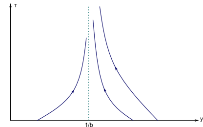
Figure 4: Structure of the characteristic curves.

5.2 Self-similarity when $\gamma+\lambda\leq 0$, $\gamma<-1$

In Section 3 we showed that when $\gamma+\lambda\leq 0$, $\gamma<-1$ and $\gamma+2\lambda>1$, equation (1.1) is compatible with a self-similar behaviour with the following scaling properties:

$$[x]=\left[\frac{t}{M_{\gamma+\lambda}}\right]^{\frac{1}{1-(\gamma+\lambda)}}\quad\text{ and }\quad[f]=\frac{[t]}{\left[\frac{t}{M_{\gamma+\lambda}}\right]^{\frac{2}{1-(\gamma+\lambda)}}}.$$ (5.11)

The aim of this Section is to study these self-similar solutions and check that they are consistent with the scenario derived in Section 3.

Time dependent equation in self-similar variables

Since the natural scaling for the anomalous self-similar solutions are the ones in (5.11), we consider the following self-similar change of variables in equation (2.5)

$$f(t,x)=\frac{t}{\left(\frac{t}{M_{\gamma+\lambda}}\right)^{\frac{2}{1-(\gamma+\lambda)}}}\Phi(\tau,\xi)\quad\text{ with }\ \xi=\frac{x}{\left(\frac{t}{M_{\gamma+\lambda}}\right)^{\frac{1}{1-(\gamma+\lambda)}}}\ \text{ and }\ \tau=\ln(t).$$ (5.12)

Substituting (5.12) in equation (2.5), we deduce that the function $\Phi$ satisfies the following equation

$$\partial_{\tau}\Phi(\tau,\xi)-\frac{1+(\gamma+\lambda)}{1-(\gamma+\lambda)}\Phi(\tau,\xi)-\frac{\xi\partial_{\xi}\Phi(\tau,\xi)}{1-(\gamma+\lambda)}+\frac{2}{1-(\gamma+\lambda)}\left(\frac{\partial_{\tau}M_{\gamma+\lambda}}{M_{\gamma+\lambda}}\right)\Phi(\tau,\xi)$$ (5.13)

$$+\frac{1}{1-(\gamma+\lambda)}\left(\frac{\partial_{\tau}M_{\gamma+\lambda}}{M_{\gamma+\lambda}}\right)\xi\partial_{\xi}\Phi(\tau,\xi)+\partial_{\xi}\left(\xi^{\gamma+\lambda}\Phi(\tau,\xi)\right)=e^{-\frac{\gamma+2\lambda-1}{1-(\gamma+\lambda)}\tau}\left(M_{\gamma+\lambda}\right)^{\frac{1-\gamma}{1-(\gamma+\lambda)}}(\mathbb{K}\Phi)(\tau,\xi)$$

for $\tau>0$ and $\xi>0$.

Notice that, since $\gamma+2\lambda>1$, the contribution to the coagulation operator term is negligible compared to the growth term. This is in agreement with the dimensional considerations performed in Section 3 and with the fact that $M_{0}\rightarrow\infty$ as time goes to infinity. As explained in Section 3, we expect $M_{\gamma+\lambda}$ to increase at most logarithmically, in particular as in (3.8). This implies that

$$\partial_{\tau}M_{\gamma+\lambda}=t\partial_{t}M_{\gamma+\lambda}\ll M_{\gamma+\lambda}\text{ as }\tau=\ln(t)\rightarrow\infty.$$ (5.14)

Moreover, since equation (2.5) is compatible with the existence of self-similar solutions, we make the ansatz: we assume that $\Phi(\tau,\cdot)\rightarrow\Phi_{\infty}$ as $\tau\rightarrow\infty$. Using the fact that $\gamma+2\lambda>1$, the self-similar ansatz and (5.14), we deduce that the self-similar profile $\Phi_{\infty}$ is the solution to the following equation

$$-\frac{1+\gamma+\lambda}{1-(\gamma+\lambda)}\Phi_{\infty}(\xi)-\frac{1}{1-(\gamma+\lambda)}\xi\partial_{\xi}\Phi_{\infty}(\xi)+\partial_{\xi}\left(\xi^{\gamma+\lambda}\Phi_{\infty}(\xi)\right)=0,\quad\text{ for }\xi\geq 0.$$ (5.15)

We now compute $\Phi_{\infty}$ and then we show that the self-similar ansatz is compatible with (5.14).

The self-similar profile

The function $\Phi_{\infty}$ defined as

$$\Phi_{\infty}(\xi)=\frac{C}{\xi^{\gamma+\lambda}}\exp\left(\int_{0}^{\xi}\frac{1}{\left(1-(\gamma+\lambda)-\eta^{1-(\gamma+\lambda)}\right)}\frac{d\eta}{\eta^{\gamma+\lambda}}\right)$$

and such that $\Phi_{\infty}(\xi)=0$ for every $\xi>\xi^{*}$, with $\xi^{*}:=(1-(\gamma+\lambda))^{\frac{1}{1-(\gamma+\lambda)}}$, satisfies (5.15) in weak sense. Here $C$ is the normalization constant given by

$$\frac{1}{C}:=\int_{0}^{\xi^{*}}\frac{1}{\xi^{\gamma+\lambda}}\exp\left(\int_{0}^{\xi}\frac{1}{\left(1-(\gamma+\lambda)-\eta^{1-(\gamma+\lambda)}\right)}\frac{d\eta}{\eta^{\gamma+\lambda}}\right)d\xi.$$

Therefore, $\Phi_{\infty}$ is the self-similar profile.

The properties of the self-similar profile are consistent with the ansatz (5.14)

Now we check that the properties of the self-similar profile $\Phi_{\infty}$ are consistent with (5.14). To this end we use a matched asymptotics argument to combine the behaviour of $f$ in the inner region with the behaviour of $f$ in the outer region.

It has been shown in Section 4 that, in the inner region, when $1\ll n\ll L(t)=t^{\frac{1}{1-(\gamma+\lambda)}}$, the solution $f(t)$ to equation (2.5) behaves as the function $c_{n}$ given by (4.6). Thanks to the Ansatz (5.14) and to the fact that $\gamma+2\lambda>1$ we also have that $M_{\gamma+\lambda}^{\frac{2}{\gamma+2\lambda}}\ll t^{\frac{1}{1-(\gamma+\lambda)}}$ as $t\rightarrow\infty$.

We can therefore consider the following regime: $M_{\gamma+\lambda}^{\frac{2}{\gamma+2\lambda}}\ll n\ll t^{\frac{1}{1-(\gamma+\lambda)}}$ as $t\rightarrow\infty$, where we have that

$$c_{n}(t)\simeq\frac{\left[\left(2\pi\right)^{\frac{\gamma}{2}+\lambda}K\right]\left(M_{\gamma+\lambda}\right)^{2}}{n^{\gamma+\lambda}}\exp\left(-\left(M_{\gamma+\lambda}\right)^{\frac{2}{\gamma+2\lambda}}A_{\gamma+2\lambda}\right)$$ (5.16)

as $t\rightarrow\infty$ and where

$$A_{\gamma+2\lambda}:=\int_{0}^{\infty}\log\left(1+\frac{1}{y^{\gamma+2\lambda}}\right)dy.$$

On the other hand, when $n\approx t^{\frac{1}{1-(\gamma+\lambda)}}$ we expect the solution $f$ to equation (2.5) to behave like (5.12). Since we also have that $\Phi(\tau,\cdot)\rightarrow\Phi_{\infty}$ as $\tau$ tends to infinity, then

$$f(t,n)=t^{-\frac{1+\gamma+\lambda}{1-(\gamma+\lambda)}}M_{\gamma+\lambda}^{\frac{2}{1-(\gamma+\lambda)}}\Phi_{\infty}\left(\xi\right)\quad\text{ with }\ \xi=n\left(\frac{M_{\gamma+\lambda}}{t}\right)^{\frac{1}{1-(\gamma+\lambda)}}.$$

Matching the inner region with the outer region and taking into account that $\Phi_{\infty}(\xi)\sim\xi^{-(\gamma+\lambda)}$ as $\xi\rightarrow 0^{+}$, we deduce that

$$\frac{\left[\left(2\pi\right)^{\frac{\gamma}{2}+\lambda}K\right]\left(M_{\gamma+\lambda}\right)^{2}}{n^{\gamma+\lambda}}\exp\left(-\left(M_{\gamma+\lambda}\right)^{\frac{2}{\gamma+2\lambda}}A_{\gamma+2\lambda}\right)=t^{-\frac{1+\gamma+\lambda}{1-(\gamma+\lambda)}}M_{\gamma+\lambda}^{\frac{2}{1-(\gamma+\lambda)}}n^{-(\gamma+\lambda)}\left(\frac{t}{M_{\gamma+\lambda}}\right)^{\frac{\gamma+\lambda}{1-(\gamma+\lambda)}}.$$

This implies that for a suitable constant $c>0$ we have that

$$cM_{\gamma+\lambda}^{-\frac{\gamma+\lambda}{1-(\gamma+\lambda)}}\exp\left(-M_{\gamma+\lambda}^{\frac{2}{\gamma+2\lambda}}A_{\gamma+2\lambda}\right)=t^{-\frac{1}{1-(\gamma+\lambda)}}$$

and hence,

$$M_{\gamma+\lambda}\simeq\left(\frac{1}{A_{\gamma+2\lambda}}\ln\left(ct^{\frac{1}{1-(\gamma+\lambda)}}\right)\right)^{\frac{\gamma+2\lambda}{2}}\text{ as }t\rightarrow\infty.$$

This is in agreement with the Ansatz (5.14) as $t\rightarrow\infty$ and with (3.8).

Comparison with the physical literature

The result for $\gamma+2\lambda>1$, $\gamma<-1$ and $\gamma+\lambda\leq 0$ obtained in this section is consistent with the results obtained in [12] and in [13]. In these references, the coagulation equation with a source of monomers with the kernel

$$K_{ij}=i^{-\mu}+j^{-\mu}$$

has been considered. This corresponds, in our notation, to $\gamma+\lambda=0$ and $\mu=\lambda=-\gamma>1$. In these papers, it is also found that $c_{n}$ behaves as (5.16) with $M_{0}=M_{\gamma+\lambda}$. Moreover, they obtain the following growth rate for the $0$-th moment

$$M_{\gamma+\lambda}=M_{0}\simeq\left\{\frac{1}{A_{\gamma+2\lambda}}\ln\left[t\ln\left(\frac{\ln t}{A_{\gamma+2\lambda}}\right)^{1-3\lambda/2}\right]\right\}^{\lambda/2}$$

as $t\rightarrow\infty$. This is in agreement with (3.8).

5.3 Self-similarity when $\gamma=-1$

In Section 3 we showed that when $\gamma=-1$ and $\gamma+2\lambda>1$, equation (1.1) is compatible with a self-similar behaviour. In particular we expect the following scaling properties:

$$[x]=[t][\ln(t)]^{\frac{1}{2}}\quad\text{ and }\quad[f]=\frac{1}{[t\ln(t)]}.$$ (5.17)

The aim of this Section is to study the self-similar solutions for equation (2.5) corresponding to the above scalings.

Time dependent equation in self-similar variables

The scaling properties (5.17) suggest to make the following change of variables in equation (2.5)

$$f(t,x)=\frac{1}{t\ln t}\Phi(\tau,y)\quad\text{ with }\quad\tau=\ln t\ \text{ and }\ y=\frac{x}{t\ln(t)^{1/2}}.$$

By elementary computations, we deduce that $\Phi$ satisfies the following equation

$$\partial_{\tau}\Phi(\tau,y)+\partial_{y}\left[\left(\frac{y^{\gamma+\lambda}}{M_{\gamma+\lambda}}-y\right)\Phi(\tau,y)\right]-\frac{1}{2y\tau}\partial_{y}(y^{2}\Phi(\tau,y))=\frac{1}{\tau}\mathbb{K}(\Phi)(\tau,y).$$ (5.18)

Notice that, due to the factor $1/\tau$ in front of it, we expect the contribution of the coagulation operator to the dynamics to be weaker than the one of the growth term. Differently from what happens when $\gamma<-1$, the coagulation term is not exponentially decreasing in time. This explains in particular why we have a different scenario compared to the one that we have when $\gamma+\lambda>0$ and $\gamma<-1$, although in both cases we have that the number of particles tends to a constant as time tends to infinity and that the $M_{\gamma+\lambda}$ grows in time like a power law.

We now make the self-similar ansatz, hence we assume that $\Phi(\tau,\cdot)\rightarrow\Phi_{\infty}$ as $\tau$ tends to infinity. Using the fact that some of the terms in equation (5.18) decay in time as $1/\tau$ we take formally the limit as $\tau$ tends to infinity in equation (5.18) to deduce that $\Phi_{\infty}$ should satisfy the following equation

$$\partial_{y}\left[\left(\frac{y^{\gamma+\lambda}}{M_{\gamma+\lambda}}-y\right)\Phi_{\infty}(y)\right]=0.$$ (5.19)

In the next section we study the form of $\Phi_{\infty}$.

The self-similar profile

In this section we want to study the solutions to equation (5.19). Since we also want $\int_{\mathbb{R}_{*}}x\Phi_{\infty}(x)dx=1$ we deduce that

$$\Phi_{\infty}(y)=\frac{1}{a}\delta(y-a)$$ (5.20)

for some $a>0$. We stress that this case is similar to the one studied in Section 5.1 (cf. equation (5.4)). In that case, we compute the value of $b$ in (5.6) using the fact that $M_{0}$ converges to a constant in time, implying that $b=M_{0,\infty}$ (see (5.6)) and it hence depends on the zeroth moment of the initial datum.

The same type of argument does not work with the set of parameters considered in this section and we will have to adapt it to this case using the precise asymptotic behaviour of $M_{0}$. We therefore analyse in more detail the dynamics for large times. A sketch of the interaction between the growth term and the coagulation term in equation (5.18) is presented in Figure 5. As we will see later, even if the coagulation term tends to zero as time tends to infinity, it will determine the value of $a$ in (5.20).

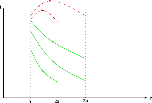
Figure 5: In this figure, the solid line describes the characteristic curves transporting particles to size $y=a$. The dashed line, instead, represents the effect of the coagulation term.

To this end, using the fact that we expect $\Phi(\tau,\cdot)\rightarrow\frac{1}{a}\delta(\cdot-a)$ and using the homogeneity of the kernel $K$, we consider the following approximation for the coagulation operator

$$\mathbb{K}(\Phi)(\tau,y)\simeq\frac{1}{2a^{2}}\int_{0}^{y}K\left(y-x,x\right)\delta\left(y-x-a\right)\delta\left(x-a\right)dx-\frac{1}{a}\Phi\left(\tau,y\right)\int_{0}^{\infty}K(x,y)\delta(x-a)dx$$

$$\simeq\frac{1}{2a^{3}}K(1,1)\delta(y-2a)-\frac{1}{a^{2}}K(1,1)\Phi(\tau,y).$$

Using this approximation for the coagulation operator in equation (5.18), we deduce that

$$\partial_{\tau}\Phi(\tau,y)+\partial_{y}\left[\left(\frac{y^{\gamma+\lambda}}{M_{\gamma+\lambda}}-y-\frac{1}{2\tau}y\right)\Phi(\tau,y)\right]=\frac{K(1,1)}{2a^{3}\tau}\delta(y-2a)+\frac{1}{2\tau}\Phi(\tau,y)-\frac{1}{a^{2}\tau}K(1,1)\Phi(\tau,y)$$

Since the coagulation term in equation (5.18) is of order $1/\tau$ and since the growth term, as time tends to infinity, is negative for sizes larger that $2a$, we can assume that $\Phi(\tau,\cdot)$ is equal to zero on the set $(2a,\infty)$. As a consequence, we can reformulate the equation for $\Phi$ as

$$\partial_{\tau}\Phi(\tau,y)+\partial_{y}\left[\left(\frac{y^{\gamma+\lambda}}{M_{\gamma+\lambda}}-y-\frac{1}{2\tau}y\right)\Phi(\tau,y)\right]=\frac{1}{2\tau}\Phi(\tau,y)-\frac{1}{a^{2}\tau}K(1,1)\Phi(\tau,y)\quad\text{ for }y<2a$$ (5.21)

with the following boundary condition at $y=2a$

$$-\left[\frac{(2a)^{\gamma+\lambda}}{M_{\gamma+\lambda}}-2a-\frac{a}{\tau}\right]\Phi(\tau,2a)=\frac{K(1,1)}{2a^{3}\tau},$$ (5.22)

which is obtained by integrating the above equation over $(2a,\infty)$.

Integrating equation (5.21) from $0$ to $2a$, using the boundary condition (5.22) and using the fact that $M_{0}$ approaches to a constant as time goes to infinity, we deduce that we should have

$$\left(\frac{K(1,1)}{a^{2}\tau}-\frac{1}{2\tau}\right)\int_{0}^{\infty}\Phi(\tau,y)dy=\frac{K(1,1)}{2a^{3}\tau}.$$

Using again the approximation $\Phi(\tau,\cdot)\simeq\frac{1}{a}\delta(\cdot-a)$, and hence the fact that $\int_{\mathbb{R}_{*}}\Phi(\tau,x)dx\simeq\frac{1}{a}$, we deduce that

$$a^{2}=K(1,1).$$ (5.23)

Equation (5.21) then reduces to

$$\partial_{\tau}\Phi(\tau,y)+\left(\frac{y^{\gamma+\lambda}}{M_{\gamma+\lambda}}-y-\frac{y}{2\tau}\right)\partial_{y}\Phi(\tau,y)+\left[(\gamma+\lambda)\frac{y^{\gamma+\lambda-1}}{M_{\gamma+\lambda}}-1\right]\Phi(\tau,y)=0\quad\text{ for }y<2a$$ (5.24)

with the following boundary condition at $y=2a$

$$-\left[\frac{(2a)^{\gamma+\lambda}}{M_{\gamma+\lambda}}-2a-\frac{a}{\tau}\right]\Phi(\tau,2a)=\frac{1}{2a\tau}.$$ (5.25)

Convergence to the self-similar profile

We study equation (5.24) with the boundary condition (5.25) and initial value $\Phi_{0}=\Phi(\tau_{0},\cdot)$ at time $\tau=\tau_{0}\ll 1$, supported in $y<2a$. The families of characteristics for equation (5.24) are

$$\frac{dY}{d\tau}=\frac{Y^{\gamma+\lambda}}{M_{\gamma+\lambda}}-Y-\frac{Y}{2\tau},\quad\text{ for }\tau\geq\tau_{0}\ \text{ with }\ Y(\tau_{0},y_{0})=y_{0}\in(0,2a)$$

and

$$\frac{d\overline{Y}}{d\tau}=\frac{\overline{Y}^{\gamma+\lambda}}{M_{\gamma+\lambda}}-\overline{Y}-\frac{\overline{Y}}{2\tau},\quad\text{ for }\tau\geq\overline{\tau}\ \text{ with }\ \overline{Y}(\overline{\tau},\overline{\tau})=2a.$$

Here $\overline{Y}(\tau,\overline{\tau})=Y(\tau-\overline{\tau},2a)$ where $\bar{\tau}>\tau_{0}$. Hence, the solution $\Phi$ to equation (5.24) satisfies

$$\Phi(\tau,Y(\tau,y_{0}))=\Phi_{0}(y_{0})e^{\int_{\tau_{0}}^{\tau}\left(1-(\gamma+\lambda)\frac{Y(s,y_{0})^{\gamma+\lambda-1}}{M_{\gamma+\lambda}}\right)ds}$$

and using the boundary condition (5.25) we obtain

$$\Phi(\tau,\overline{Y}(\tau,\overline{\tau}))=\Phi(\overline{\tau},2a)e^{\int_{\overline{\tau}}^{\tau}\left(1-(\gamma+\lambda)\frac{\overline{Y}(s,\overline{\tau})^{\gamma+\lambda-1}}{M_{\gamma+\lambda}}\right)ds}=\frac{1}{2a^{2}\overline{\tau}}\frac{1}{(2-2^{\gamma+\lambda}+\frac{1}{\overline{\tau}})}e^{\int_{\overline{\tau}}^{\tau}\left(1-(\gamma+\lambda)\frac{\overline{Y}(s,\overline{\tau})^{\gamma+\lambda-1}}{M_{\gamma+\lambda}}\right)ds}.$$ (5.26)

The contribution of the initial datum $\Phi_{0}$ as time tends to infinity is negligible. Indeed, it is possible to show that

$$\int_{(0,2a)}Y(\tau,y_{0})\Phi(\tau,Y(\tau,y_{0}))dy_{0}\rightarrow 0\text{ as }\tau\rightarrow\infty.$$

Therefore, the asymptotic behaviour of $\Phi$ is given by the long-time behaviour of (5.26). To study the long-time behaviour of $\overline{Y}$, we approximate the equation for the characteristics as

$$\frac{d\overline{Y}}{d\tau}=\frac{\overline{Y}^{\gamma+\lambda}}{a^{\gamma+\lambda-1}}-\overline{Y},\quad\text{ for }\tau\geq\overline{\tau}\ \text{ with }\ \overline{Y}(\overline{\tau},\overline{\tau})=2a$$

where we are using the fact that as $\tau-\overline{\tau}\rightarrow\infty$ we have $M_{\gamma+\lambda}\simeq a^{\gamma+\lambda-1}$ because we expect $\Phi(\tau,\cdot)$ to converge to $\frac{1}{a}\delta_{a}$. Notice that as $\tau-\overline{\tau}\rightarrow\infty$ we have that $\overline{Y}(\tau,\overline{\tau})\rightarrow a$.

Linearizing the ODE for $\overline{Y}$ around the equilibrium $a$, we deduce that as $\tau-\overline{\tau}\rightarrow\infty$ we have that

$$\overline{Y}(\tau,\overline{\tau})=Y(\tau-\overline{\tau},2a)\simeq a+Ke^{-[1-(\gamma+\lambda)](\tau-\overline{\tau})},$$

where the constant $K\simeq a$ depends on $\gamma+\lambda$ and on $a$. This implies that if $\xi=\overline{Y}(\tau,\overline{\tau})$, then, since $a<\xi<2a$ and $0<\frac{\xi-a}{K}<1$, we have that

$$\overline{\tau}=\tau+\frac{1}{1-(\gamma+\lambda)}\ln\left(\frac{\xi-a}{K}\right)\leq\tau.$$

As a consequence, equality (5.26) can be rewritten as

$$\Phi(\tau,\xi)\simeq\frac{1}{2a^{2}\overline{\tau}}\frac{1}{(2-2^{\gamma+\lambda}+\frac{1}{\overline{\tau}})}e^{(1-\gamma-\lambda)(\tau-\overline{\tau})}\simeq\frac{1}{2a^{2}\overline{\tau}}\frac{1}{(2-2^{\gamma+\lambda})}\frac{K}{\xi-a}$$ (5.27)

for large values of $\tau$ and $\overline{\tau}$ and for $\xi>a$. This is compatible with $\Phi(\tau,\cdot)\rightarrow\Phi_{\infty}$ as $\tau\rightarrow\infty$ only when $\overline{\tau}\approx\tau$. Instead when $\overline{\tau}\ll\tau$, in particular, if

$$\tau\approx\frac{1}{1-(\gamma+\lambda)}\left|\log\left(\frac{\xi-a}{K}\right)\right|\,,$$

the approximation is not valid. Indeed, according to (5.27), we would have that $M_{0}$ tends to infinity as $\tau$ tends to infinity.

This argument partially supports the convergence towards the self-similar profile (5.20) where $a^{2}=K(1,1)$. However, a complete result would require more detailed analysis.

6 Conjectures on the self-similar behaviour when $\gamma+2\lambda=1$

As explained in the previous Sections, when $\gamma+2\lambda>1$, we obtained consistent asymptotic behaviour both for $\gamma>-1$, $\gamma=-1$ and $\gamma<-1$ with $M_{\gamma+\lambda}\rightarrow\infty$ as time tends to infinity. Instead, as explained in [4], in the case $\gamma>-1$, $\gamma+2\lambda=1$ there exist self-similar solutions for which the moment $M_{\gamma+\lambda}$ is constant. In the rest of this section, we first recall in Section 6.1 the results obtained in [4] for the case $\gamma>-1$, $\gamma+2\lambda=1$ and describe then in Section 6.2 a possible scenario for the behaviour of the solutions when $\gamma\leq-1$ and $\gamma+2\lambda=1$. We stress that this case is more involved than the other as the matching between the inner and outer regions is non-trivial, see Section 6.2 for more details. Figure 6 also shows that the critical line $\gamma+2\lambda=1$ is at the intersection of a number of different behaviours. There is no obvious choice between them for a dominant behaviour at the critical line which makes this case particularly challenging.

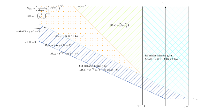
Figure 6: In this picture we show the different behaviours near the critical line $\gamma+2\lambda=1$ in the different regimes $\gamma<-1$, $\gamma=-1$ and $-1<\gamma<1$.

6.1 Comparison with previous results in the case $\gamma>-1$

Self-similarity when $\gamma+2\lambda=1$ and $\gamma>-1$

The long-time behaviour of the solutions $f$ to equation (2.5) when $\gamma+2\lambda=1$ and $\gamma>-1$ is studied in [4]. In particular, it is explained there, via formal arguments, that the solutions $f$ approach, as time tends to infinity, the solution $\overline{f}$ to equation (2.6) in the inner region where $x\approx 1$. On the other hand, the dimensional analysis in Section 3 shows that we can expect the long-time behaviour of the solutions to equation (2.5) to be self similar and with the scalings given by (2.2). The self-similar profiles $\Phi$, then satisfy the following equation

$$-\frac{3+\gamma}{1-\gamma}\Phi\left(\xi\right)-\frac{2}{1-\gamma}\xi\partial_{\xi}\Phi\left(\xi\right)+\frac{1}{M_{\gamma+\lambda}}\frac{\partial}{\partial\xi}\left(\xi^{\gamma+\lambda}\Phi\left(\xi\right)\right)=\mathbb{K}\left[\Phi\right]\left(\xi\right)\ \ ,\ \ \xi>0.$$ (6.1)

In [4] the existence of these self-similar solutions is proven and their properties are analysed. In particular, it is proven in there that the self-similar profiles are zero in an interval near the origin and that they decay exponentially for large sizes. While the exponential decay for large sizes is typically seen in the theory of self-similar solutions for coagulation equations, the fact that the self-similar profile is zero near zero is very peculiar to the coagulation equation with source and to the assumption $\gamma+2\lambda\geq 1$.

In the rest of the section, we analyse the possibilities of having self-similar solutions of the form (2.2) with $\Phi$ satisfying (6.1) when $\gamma+2\lambda=1$, $\gamma\leq-1$.

The argument applied for $\gamma+2\lambda>1$ and $\gamma+\lambda\leq 0$ breaks down as $\gamma+2\lambda\rightarrow 1^{+}$

The analysis done in Section 5.2 for $\gamma+2\lambda>1$ and $\gamma+\lambda\leq 0$ shows that in that case the self-similar profile $\Phi_{\infty}$ is such that $\Phi_{\infty}(\xi)\sim\xi^{-(\gamma+\lambda)}$ as $\xi\rightarrow 0.$ Since this depends only on the sign of $\gamma+\lambda$, taking the limit as $\gamma+2\lambda\rightarrow 1^{+}$, we would expect the same behaviour for the self-similar profile corresponding to the case $\gamma+2\lambda=1$ and $\gamma\leq-1$ (assuming that this self-similar profile exists).

We recall that the dimensional analysis made in Section 3 for $\gamma+2\lambda>1$ and $\gamma+\lambda\leq 0$, gives the characteristic length (3.7) and implies that $M_{\gamma+\lambda}$ is logarithmically increasing in time. The dimensional analysis is valid also when $\gamma+2\lambda=1$ and $\gamma\leq-1$. Therefore, if a self-similar solution exists it should have the following scalings

$$x=\xi\left(\frac{t}{M_{\gamma+\lambda}}\right)^{\frac{1}{1-(\gamma+\lambda)}}\quad f(t,x)=\frac{t}{\left(\frac{t}{M_{\gamma+\lambda}}\right)^{\frac{2}{1-\gamma-\lambda}}}\Phi(\tau,\xi).$$

The function $\Phi$, then, should satisfy the following equation

$$\partial_{\tau}\Phi(\tau,\xi)-\frac{1+(\gamma+\lambda)}{1-(\gamma+\lambda)}\Phi(\tau,\xi)-\frac{\xi\partial_{\xi}\Phi(\tau,\xi)}{1-(\gamma+\lambda)}+\frac{2}{1-(\gamma+\lambda)}\left(\frac{\partial_{\tau}M_{\gamma+\lambda}}{M_{\gamma+\lambda}}\right)\Phi(\tau,\xi)$$ (6.2)

$$+\frac{1}{1-(\gamma+\lambda)}\left(\frac{\partial_{\tau}M_{\gamma+\lambda}}{M_{\gamma+\lambda}}\right)\xi\partial_{\xi}\Phi(\tau,\xi)+\partial_{\xi}\left(\xi^{\gamma+\lambda}\Phi(\tau,\xi)\right)=\left(M_{\gamma+\lambda}\right)^{\frac{1-\gamma}{1-(\gamma+\lambda)}}(\mathbb{K}\Phi)(\tau,\xi)$$

for $\tau>0$ and $\xi>0$. The dominant term in equation (6.2) would be the coagulation term, in contrast with the scenarios described in Section 5 for $\gamma+2\lambda>1$.

On the other hand, the asymptotics derived in Section 4.1 for the case $\gamma+2\lambda>1$ is based on the fact that, when $\gamma+2\lambda\geq 1$, the flux of particles $J_{c}(M_{\gamma+\lambda})$ is given by (4.6). When $\gamma+2\lambda=1$, this reduces to

$$J_{c}(M_{\gamma+\lambda})(x)=\frac{\left[\left(2\pi\right)^{\frac{1}{2}}K\right]\left(M_{\gamma+\lambda}\right)^{2}}{x^{\gamma+\lambda}\sqrt{1+\frac{\left(M_{\gamma+\lambda}\right)^{2}}{x}}}\exp\left(-\left(M_{\gamma+\lambda}\right)^{2}\int_{0}^{\frac{x}{(M_{\gamma+\lambda})^{2}}}\log\left(1+\frac{1}{y}\right)dy\right).$$

In order to match the inner behaviour with the outer self-similar behaviour, we consider in Section 5.2 that $M_{\gamma+\lambda}\ll x\ll t^{\frac{1}{1-(\gamma+\lambda)}}$, as $t\to\infty$ in the formula for the flux of particles. When $\gamma+2\lambda>1$, we have that

$$\int_{0}^{\frac{x}{(M_{\gamma+\lambda})^{\frac{2}{\gamma+2\lambda}}}}\log\left(1+\frac{1}{y^{\gamma+2\lambda}}\right)dy\rightarrow A_{\gamma+2\lambda}$$

as $\frac{x}{(M_{\gamma+\lambda})^{\frac{2}{\gamma+2\lambda}}}\rightarrow\infty$, where $A_{\gamma+2\lambda}:=\int_{0}^{\infty}\log\left(1+\frac{1}{y^{\gamma+2\lambda}}\right)dy<\infty$. Then, for large $x$, the flux of particles behaves like

$$J_{c}(M_{\gamma+\lambda})\approx\left(2\pi\right)^{\frac{\gamma+2\lambda}{2}}K\left(M_{\gamma+\lambda}\right)^{2}\exp\left(-\left(M_{\gamma+\lambda}\right)^{2}A_{\gamma+2\lambda}\right).$$

However, the constant $A_{\gamma+2\lambda}$ is equal to $\infty$ when $\gamma+2\lambda=1$. As a consequence the matching argument explained in Section 5.2 breaks down in that case. The case $\gamma+2\lambda=1$ and $\gamma=-1$ has already been considered in [12] and [13], where a logarithmic correction for $M_{\gamma+\lambda}$ is suggested.

6.2 Conjecture on the existence of self-similar solutions when $M_{\gamma+\lambda}<\infty$

In this section, we analyse the possibility of having self-similar solutions when $M_{\gamma+\lambda}$ is constant. When $\gamma+2\lambda=1$ and $\gamma\leq-1$, we could expect, as explained in Section 2.3, the solutions to equation (1.1) to behave in the inner region ($x\approx 1$) as the solution $\overline{f}$ to (2.6), and, in the outer region ($x\approx t^{\frac{2}{1-\gamma}}$), as self-similar solutions to equation (2.5) of the form (2.2). We check here that this scenario does not lead to any contradictions. However, showing that the long-time behaviour to equation (1.1) is indeed self-similar also when $\gamma+2\lambda=1$ and $\gamma\leq-1$ would need a careful analytic study of the existence of self-similar solutions which we are not going to do here.

Matching between the inner and outer region

Since we are assuming that $M_{\gamma+\lambda}<\infty$, we deduce that the behaviour in the inner region is described by the solution $\overline{f}$ to equation (2.6). The asymptotics as $x$ tends to infinity of $\overline{f}$ suggest that if $M_{\gamma+\lambda}^{in}\geq 1$ then

$$\overline{f}(x)=x^{-\frac{\gamma+3}{2}}\varepsilon(x)$$ (6.3)

where $\varepsilon(x)\rightarrow 0$ as $x\rightarrow\infty$.

In the outer region, when $x\approx t^{\frac{2}{1-\gamma}}$, we expect the solution $f$ to equation (1.1) to behave, for large times, as the self-similar solutions of the form (2.2) where the self-similar profile $\Phi$ satisfies equation (6.1).

We now present asymptotic analysis suggesting that the self-similar profile may behave in two different ways, when $x\ll t^{\frac{2}{1-\gamma}}$, depending on whether $M_{\gamma+\lambda}=1$ or $M_{\gamma+\lambda}\neq 1$. Precisely, we expect that if $M_{\gamma+\lambda}=1$, then

$$\Phi(\xi)\approx\frac{1}{\xi^{\frac{\gamma+3}{2}}\left(\log(\frac{1}{\xi})\right)^{2}},\quad\xi\rightarrow 0$$ (6.4)

while if $M_{\gamma+\lambda}\neq 1$, then

$$\Phi(\xi)\approx\frac{1}{\xi^{\frac{\gamma+3}{2}}}\frac{1}{\xi^{(M_{\gamma+\lambda}^{2}-1)}},\quad\xi\rightarrow 0.$$ (6.5)

Although, if $\Phi$ behaves like (6.5) and $M_{\gamma+\lambda}>1$, then we would have that the $\gamma+\lambda$ moment of $\Phi$ would be equal to infinity, leading to a contradiction. Therefore, we conjecture $M_{\gamma+\lambda}\leq 1$. Even if we also know that $M_{\gamma+\lambda}=\frac{1}{M_{\gamma+\lambda}^{in}}$ and that $M_{\gamma+\lambda}^{in}\geq 1$, we do not know how to determine the value of $M_{\gamma+\lambda}\leq 1$. This could be studied as an eigenvalue problem for equation (6.1) that we do not plan to solve here.

We now explain how we derive (6.4) and (6.5). Since we are assuming that $M_{\gamma+\lambda}<\infty$, then we must have $\Phi(\xi)<\xi^{-\frac{3+\gamma}{2}}$ for small $\xi$. Therefore, considering only the leading terms as $\xi\rightarrow 0$ in equation (6.1) we deduce the following approximate equation

$$\frac{1}{M_{\gamma+\lambda}}\frac{\partial}{\partial\xi}\left(\xi^{\gamma+\lambda}\Phi\left(\xi\right)\right)=\mathbb{K}\left[\Phi\right]\left(\xi\right)\text{ as }\xi\rightarrow 0.$$

We now multiply by $\xi$ and integrate from $0$ to $z$ all the terms in the above equation. Using also the fact that $\lim_{z\rightarrow 0}J[\Phi](z)=0$, we rewrite the approximate equation in the following mass flux form

$$J[\Phi](z)=-\frac{1}{M_{\gamma+\lambda}}z^{\gamma+\lambda+1}\Phi(z)+\frac{1}{M_{\gamma+\lambda}}\int_{0}^{z}x^{\gamma+\lambda}\Phi(x)dx.$$ (6.6)

Let us define the function $H(z):=\int_{0}^{z}x^{1-\lambda}\Phi(x)dx$. We now approximate $J$ with similar arguments to the one presented in Section 4.2. Indeed, assuming that $z\ll 1$, using the asymptotics (1.8) for the kernel and using the fact that $M_{\gamma+\lambda}<\infty$, we deduce that

$$J[\Phi](z)\approx\int_{0}^{z}\int_{z}^{\infty}xK(x,y)\Phi(y)\Phi(x)dydx\text{ as }z\rightarrow 0.$$ (6.7)

Then, assuming that $M_{\gamma+\lambda}=1$, equation (6.6) can be rewritten as

$$(H(z))^{2}\approx z\frac{dH(z)}{dz}.$$

This implies that $H(z)\approx\frac{1}{\log\left(1/z\right)}$ as $z$ tends to zero and, hence by differentiation, we deduce (6.4).

When, instead, $M_{\gamma+\lambda}<1$, we can use (6.7) to rewrite equation (6.6) in the following approximated form:

$$(1-M_{\gamma+\lambda}^{2})H(z)\approx z\frac{dH(z)}{dz}.$$

This implies that $H(z)\approx z^{1-M_{\gamma+\lambda}^{2}}$ and hence (6.5) follows.

Notice that (6.4) and (6.5) with $M_{\gamma+\lambda}\leq 1$ are compatible with (6.3) with $M_{\gamma+\lambda}^{in}\geq 1$. Therefore, this scenario suggests that, in the case of the critical exponents $\gamma+2\lambda=1$ and $\gamma\leq-1$, the long term behaviour of the solution $f$ to equation (1.1) could be given by the self-similar solutions of the form (2.2) for equation (2.5), assuming that these solutions exist.

Relation with the non-existence result in [4]

We recall that in [4] it has been proven that, when $\gamma+2\lambda>1$ and $\gamma>-1$, self-similar solutions for equation (2.5) exist and that the self-similar profile $\Phi$ is zero near the origin. On the other side it has been proven there that self-similar solutions of the form (2.2) to equation (2.5) with $\int_{0}^{1}x^{-\lambda}\Phi(x)dx<\infty$ do not exist. The conjecture we make here is not in contradiction with the non-existence result stated in [4]. Indeed, the condition near the origin, (6.4) as well as (6.5), guarantees that

$$\int_{0}^{1}\xi^{-\lambda}\Phi(\xi)d\xi=\infty$$

for any choice of $M_{\gamma+\lambda}\geq 1$.

It is interesting to compare the behaviour described here for $\gamma+2\lambda=1$ and $\gamma\leq-1$ to the one $\gamma+2\lambda<1$, see [8]. In that case, the existence of self-similar solutions is proven for the coagulation equation with a constant influx coming from the origin. This condition is reflected in the behaviour of the self-similar profile near the origin, i.e., $\Phi(\xi)\approx\xi^{-\frac{(\gamma+3)}{2}}$ as $\xi$ tends to zero. In the case considered here, with $\gamma+2\lambda=1$ and $\gamma\leq-1$, we obtain in (6.4) and in (6.5) the same power law behaviour but with corrections. These corrections are due to the fact that there are no fluxes from the origin.

7 Conclusions

In this work, relying also on [4], [8], we have described several examples of long-time asymptotics for the solutions to the Smoluchowski coagulation equation with source, i.e., to (1.1). This shows that the equation exhibits a very rich class of possible self-similar behaviours, depending only on the range of parameters $\gamma$ and $\lambda$ which characterize the coagulation kernel. We summarize here how the self-similar behaviour of the solutions $f$ to equation (1.1) changes when varying $\gamma$ and $\lambda$.

• When $\gamma+2\lambda<1$ we expect the following self-similar behaviour of $f$ for large $x$ and large $t$

  $$f(t,x)\sim t^{-\frac{3+\gamma}{1-\gamma}}\Phi\left(\frac{x}{t^{\frac{2}{1-\gamma}}}\right)\text{ and }\Phi(\xi)\sim\xi^{-\frac{\gamma+3}{2}}\text{ as }\xi\rightarrow 0.$$

  Rigorous results on the existence of self-similar solutions as above can be found in [8]. While numerical simulations, showing convergence to self-similarity, supported also by matching asymptotics arguments can be found in [5].

• When $\gamma+2\lambda>1$, we expect the following self-similar behaviour of $f$ for large $x$ and large $t$

  parameters	self-similar solution
  $\boldsymbol{\gamma>-1}$	$f(t,x)\sim t^{-\frac{3+\gamma}{1-\gamma}}\Phi\left(\frac{x}{t^{\frac{2}{1-\gamma}}}\right)\ \ \text{ and}\ \ \Phi(\xi)=0\ \text{ for small }\ \xi$
  $\boldsymbol{\gamma=-1}$	$f(t,x)\sim\frac{1}{at\ln t}\delta\left(\frac{x}{t(\ln(t))^{1/2}}-a\right)$
  $\boldsymbol{\gamma<-1,\,\gamma+\lambda>0}$	$f(t,x)\sim\frac{t}{\left(\frac{t}{M_{\gamma+\lambda}}\right)^{\frac{2}{1-(\gamma+\lambda)}}}\Phi\left(x{\left(\frac{M_{\gamma+\lambda}}{t}\right)^{\frac{1}{1-(\gamma+\lambda)}}}\right)$, $\Phi(\xi)\sim\xi^{-(\gamma+\lambda)}$ as $\xi\rightarrow 0$
  $\boldsymbol{\gamma<-1,\,\gamma+\lambda\leq 0}$	$f(t,x)\sim\frac{1}{bt}\delta\left(\frac{x}{t}-b\right)$

  Rigorous results on the existence of self-similar solutions when $\gamma>-1$ can be found in [4]. The analysis of the complementary cases is the main content of this paper.

• When $\gamma+2\lambda=1$ we expect the following self-similar behaviour for large values of $x$ and $t$

  parameters	self-similar solution
  $\boldsymbol{\gamma>-1}$	$f(t,x)\sim t^{-\frac{3+\gamma}{1-\gamma}}\Phi\left(\frac{x}{t^{\frac{2}{1-\gamma}}}\right)$   and    $\Phi(\xi)=0$ for small $\xi$
  $\boldsymbol{\gamma\leq-1}$	$f(t,x)\sim t^{-\frac{3+\gamma}{1-\gamma}}\Phi\left(\frac{x}{t^{\frac{2}{1-\gamma}}}\right)$ with $\Phi(\xi)\sim\frac{\xi^{-\frac{\gamma+3}{2}}}{\log\left(1/\xi\right)}$ or $\Phi(\xi)\sim\xi^{-\frac{\gamma+3}{2}+1-M_{\gamma+\lambda}}$ as $\xi\rightarrow 0$

A rigorous analysis for $\gamma+2\lambda=1$ of the existence/non-existence of standard self-similar solutions which are zero near zero can be found in [4]. Here, we have presented conjectures in the case $\gamma+2\lambda=1$ and $\gamma\leq-1$ and the solutions then have different behaviours near zero. We conjecture that, under these assumptions on the parameters $\gamma$ and $\lambda$, the characteristic length for the self-similar solutions is $L(t)=t^{\frac{2}{1-\gamma}}$. Moreover, using asymptotics analysis, we prove that the behaviour of the self-similar profile $\Phi$ near the origin depends on the value of $M_{\gamma+\lambda}$. We claim that if $M_{\gamma+\lambda}=1$ then $\Phi(\xi)\sim\frac{1}{\log\left(1/\xi\right)}\xi^{-\frac{\gamma+3}{2}}$ as $\xi\rightarrow 0$, while if $M_{\gamma+\lambda}>1$ then $\Phi(\xi)\sim\xi^{-\frac{\gamma+3}{2}}\xi^{1-M_{\gamma+\lambda}}$ as $\xi\rightarrow 0$. A rigorous analysis would be needed to prove this conjecture since our computations are not enough to determine the value of $M_{\gamma+\lambda}$.

Appendix A Some details on the justification of (4.6) (cf. Section 4.1).

We now clarify the asymptotics (4.12). We first recall that the sequence $\left\{X_{n}\right\}_{n\in\mathbb{N}}$ satisfies (4.10). It is convenient to perform the change of variables $X_{n}=\left(n!\right)^{\gamma+2\lambda}Y_{n}$ in (4.10). Noticing that $X_{1}=Y_{1}=1$ we obtain

$$Y_{n} =\frac{\left(n\right)^{\lambda}}{2}\sum_{j=1}^{n-1}K\left(n-j,j\right)\frac{\left(\left(n-j\right)!\right)^{\gamma+2\lambda}\left(\left(j\right)!\right)^{\gamma+2\lambda}}{\left(n!\right)^{\gamma+2\lambda}}Y_{n-j}Y_{j}$$

$$=\left(n\right)^{\gamma+2\lambda}\frac{K\left(n-1,1\right)\left(\left(n-1\right)!\right)^{\gamma+2\lambda}}{n^{\gamma+\lambda}\left(n!\right)^{\gamma+2\lambda}}Y_{n-1}Y_{1}+\sum_{j=2}^{n-2}K\left(n-j,j\right)\frac{\left(\left(n-j\right)!\right)^{\gamma+2\lambda}\left(\left(j\right)!\right)^{\gamma+2\lambda}}{\left(n!\right)^{\gamma+2\lambda}}Y_{n-j}Y_{j}$$

$$=\frac{K\left(n-1,1\right)}{n^{\gamma+\lambda}}Y_{n-1}+\sum_{j=2}^{n-2}K\left(n-j,j\right)\frac{\left(\left(n-j\right)!\right)^{\gamma+2\lambda}\left(\left(j\right)!\right)^{\gamma+2\lambda}}{\left(n!\right)^{\gamma+2\lambda}}Y_{n-j}Y_{j}\ .$$

We need to examine the asymptotic behaviour of $Y_{n}$ as $n\rightarrow\infty.$ We remark that we can have exponential, “subfactorial”, corrections in $Y_{n}.$ Actually, the detailed asymptotics of $Y_{n}$ might depend on the detailed asymptotics of the function $F\left(s\right)$ in (1.7) as $s\rightarrow 0$ (or $s\rightarrow 1$). We remark also that at the leading order we have $\frac{K\left(n-1,1\right)}{n^{\gamma+\lambda}}\simeq\left(\frac{n-1}{n}\right)^{\gamma+\lambda}\simeq 1-\frac{\left(\gamma+\lambda\right)}{n}$ as $n\rightarrow\infty.$ We then obtain the approximation

$$Y_{n}=\left(1-\frac{\left(\gamma+\lambda\right)}{n}\right)Y_{n-1}+\sum_{j=2}^{n-2}K\left(n-j,j\right)\frac{\left(\left(n-j\right)!\right)^{\gamma+2\lambda}\left(\left(j\right)!\right)^{\gamma+2\lambda}}{\left(n!\right)^{\gamma+2\lambda}}Y_{n-j}Y_{j}.$$ (A.1)

The first two terms in (A.1) yield an asymptotic behaviour with the form

$$Y_{n}\simeq\frac{K}{n^{\gamma+\lambda}}\text{ as }n\rightarrow\infty.$$ (A.2)

It remains to check if the terms in the sum $\sum_{j=2}^{n-2}\left[\cdot\cdot\cdot\right]$ in (A.1) provide a negligible contribution. To do this, we assume that $Y_{n-j}$ and$\ Y_{j}$ can be approximated by power laws as indicated above. We then examine the contribution of the factorial terms. We expect to have as the largest term the one with $j=2$. This term can be bounded as

$$K\left(n-2,2\right)\frac{\left(\left(n-2\right)!\right)^{\gamma+2\lambda}\left(\left(2\right)!\right)^{\gamma+2\lambda}}{\left(n!\right)^{\gamma+2\lambda}}Y_{n-2}Y_{2}\leq C\left(n\right)^{\gamma+\lambda}\left(\frac{1}{n^{2}}\right)^{\gamma+2\lambda}\frac{1}{n^{\gamma+\lambda}}\leq\frac{C}{n^{2\left(\gamma+2\lambda\right)}}.$$

The effect of this term can be estimated using that $Y_{n}-Y_{n-1}=-\frac{\left(\gamma+\lambda\right)}{n}Y_{n-1}+O\left(\frac{1}{n^{2\left(\gamma+2\lambda\right)}}\right).$ This shows that the term is of the order $\frac{C}{n^{2\left(\gamma+2\lambda\right)-1}}$ that is much smaller than the term $\frac{K}{n^{\gamma+\lambda}}$ as $n\rightarrow\infty.$ It is possible to show that the remaining terms in the sum yield a contribution smaller than $\frac{C}{n^{2\left(\gamma+2\lambda\right)}}.$ It then follows that the asymptotics (A.2) (and hence (4.12)) holds in the limit $n\rightarrow\infty$.

Arguing similarly, we now compute the asymptotics (4.6) of the solutions for large values of $n$. The approximation of (4.5) becomes

$$c_{n}\simeq\frac{\left(n\right)^{\lambda}}{\left[K\left(1,n\right)\left(n\right)^{\lambda}c_{1}+M_{\gamma+\lambda}\right]}K\left(n-1,1\right)c_{n-1}c_{1}\ \ \text{for }n\text{ sufficiently large.}$$

Using the approximation of $c_{1}$ in (4.7) we obtain

$$c_{n}\simeq\frac{\left(n\right)^{\lambda}}{\left[K\left(1,n\right)\left(n\right)^{\lambda}c_{1}+M_{\gamma+\lambda}\right]}\frac{K\left(n-1,1\right)c_{n-1}}{M_{\gamma+\lambda}}\ \ \text{for }n\text{ sufficiently large}$$ (A.3)

Assuming that this approximation is valid for $n\geq L$ with $L$ sufficiently large, we obtain the following approximation for $c_{n}$

$$c_{n}\simeq c_{L}\prod_{j=L+1}^{n}\left(\frac{\left(j\right)^{\lambda}K\left(j-1,1\right)}{\left[K\left(1,j\right)\left(j\right)^{\lambda}+\left(M_{\gamma+\lambda}\right)^{2}\right]}\right)$$

and using that $K\left(j-1,1\right)\simeq K\left(j-1,1\right)\simeq\left(j-1\right)^{\gamma+\lambda}$ for $j$ large, we get

$$c_{n}\simeq c_{L}\prod_{j=L+1}^{n}\left(\frac{\left(j-1\right)^{\gamma+\lambda}}{\left[\left(j\right)^{\gamma+\lambda}+\frac{\left(M_{\gamma+\lambda}\right)^{2}}{\left(j\right)^{\lambda}}\right]}\right)$$ (A.4)

Thus, we obtain that the approximation of the cluster concentrations $c_{n}$ given by (A.4) is valid for the range of values of $n$ for which we can use (A.3) as an approximation of (4.5).

We can use (A.4) to compute the flux of clusters towards large values of $n.$ To this end, we compute the asymptotic behaviour of the right hand side of (A.4) for large values of $M_{\gamma+\lambda}$ and $n$ that can be rewritten as

$$\prod_{j=L+1}^{n}\left(\frac{\left(j-1\right)^{\gamma+\lambda}}{\left[\left(j\right)^{\gamma+\lambda}+\frac{\left(M_{\gamma+\lambda}\right)^{2}}{\left(j\right)^{\lambda}}\right]}\right)=\exp\left(\sum_{j=L+1}^{n}\log\left(\frac{\left(j-1\right)^{\gamma+\lambda}}{\left(j\right)^{\gamma+\lambda}}\right)-\sum_{j=L+1}^{n}\log\left(1+\frac{\left(M_{\gamma+\lambda}\right)^{2}}{\left(j\right)^{\gamma+2\lambda}}\right)\right).$$

As $M_{\gamma+\lambda}\rightarrow\infty$, we can approximate the second sum inside the exponential as

$$\sum_{j=L+1}^{n}\log\left(1+\frac{\left(M_{\gamma+\lambda}\right)^{2}}{\left(j\right)^{\gamma+2\lambda}}\right)=\left(M_{\gamma+\lambda}\right)^{\frac{2}{\gamma+2\lambda}}\sum_{j=L+1}^{n}\log\left(1+\frac{1}{\left(\frac{j}{\left(M_{\gamma+\lambda}\right)^{\frac{2}{\gamma+2\lambda}}}\right)^{\gamma+2\lambda}}\right)\frac{1}{\left(M_{\gamma+\lambda}\right)^{\frac{2}{\gamma+2\lambda}}}.$$

Using the Euler-McLaurin formula $\sum_{j=m+1}^{n}f\left(j\right)=\int_{m}^{n}f\left(x\right)dx+\frac{1}{2}\left(f\left(n\right)-f\left(m\right)\right)+...$ we get

$$\sum_{j=L+1}^{n}\log\left(1+\frac{1}{\left(\frac{j}{\left(M_{\gamma+\lambda}\right)^{\frac{2}{\gamma+2\lambda}}}\right)^{\gamma+2\lambda}}\right)=\int_{L}^{n}\log\left(1+\frac{1}{\left(\frac{x}{\left(M_{\gamma+\lambda}\right)^{\frac{2}{\gamma+2\lambda}}}\right)^{\gamma+2\lambda}}\right)dx+$$

$$+\frac{1}{2}\left[\log\left(1+\frac{1}{\left(\frac{n}{\left(M_{\gamma+\lambda}\right)^{\frac{2}{\gamma+2\lambda}}}\right)^{\gamma+2\lambda}}\right)-\log\left(1+\frac{1}{\left(\frac{L}{\left(M_{\gamma+\lambda}\right)^{\frac{2}{\gamma+2\lambda}}}\right)^{\gamma+2\lambda}}\right)\right]$$ (A.5)

The next order term in the Euler-Maclaurin formula is bounded by the derivatives of the logarithmic function which give terms of order $\frac{1}{L},\ \frac{1}{n}$ or smaller terms. Therefore, these contributions tend to zero since $L\gg 1.$ However, we must keep the terms in (A) because they give relevant contributions. We will then approximate them as follows

$$\sum_{j=L+1}^{n}\log\left(1+\frac{\left(M_{\gamma+\lambda}\right)^{2}}{\left(j\right)^{\gamma+2\lambda}}\right)$$

$$=\int_{L}^{n}\log\left(1+\frac{\left(M_{\gamma+\lambda}\right)^{2}}{x^{\gamma+2\lambda}}\right)dx+\frac{1}{2}\left(\log\left(1+\frac{\left(M_{\gamma+\lambda}\right)^{2}}{n^{\gamma+2\lambda}}\right)-\log\left(1+\frac{\left(M_{\gamma+\lambda}\right)^{2}}{L^{\gamma+2\lambda}}\right)\right).$$

Using this new formula in (A.4) we would have

$$c_{n} \simeq c_{L}\left(\frac{L}{n}\right)^{\gamma+\lambda}\exp\left(-\left(M_{\gamma+\lambda}\right)^{\frac{2}{\gamma+2\lambda}}\int_{\frac{L}{\left(M_{\gamma+\lambda}\right)^{\frac{2}{\gamma+2\lambda}}}}^{\frac{n}{\left(M_{\gamma+\lambda}\right)^{\frac{2}{\gamma+2\lambda}}}}\log\left(1+\frac{1}{y^{\gamma+2\lambda}}\right)dy\right)\times$$

$$\quad\times\left(1+\frac{\left(M_{\gamma+\lambda}\right)^{2}}{L^{\gamma+2\lambda}}\right)^{\frac{1}{2}}\left(1+\frac{\left(M_{\gamma+\lambda}\right)^{2}}{n^{\gamma+2\lambda}}\right)^{-\frac{1}{2}}$$

On the other hand we have the following approximation for the integral

$$\int_{\frac{L}{\left(M_{\gamma+\lambda}\right)^{\frac{2}{\gamma+2\lambda}}}}^{\frac{n}{\left(M_{\gamma+\lambda}\right)^{\frac{2}{\gamma+2\lambda}}}}\log\left(1+\frac{1}{y^{\gamma+2\lambda}}\right)dy$$

$$\simeq\int_{0}^{\frac{n}{\left(M_{\gamma+\lambda}\right)^{\frac{2}{\gamma+2\lambda}}}}\log\left(1+\frac{1}{y^{\gamma+2\lambda}}\right)dy+\left(\gamma+2\lambda\right)\int_{0}^{\frac{L}{\left(M_{\gamma+\lambda}\right)^{\frac{2}{\gamma+2\lambda}}}}\log\left(y\right)dy$$

$$=\int_{0}^{\frac{n}{\left(M_{\gamma+\lambda}\right)^{\frac{2}{\gamma+2\lambda}}}}\log\left(1+\frac{1}{y^{\gamma+2\lambda}}\right)dy+\frac{\left(\gamma+2\lambda\right)L}{\left(M_{\gamma+\lambda}\right)^{\frac{2}{\gamma+2\lambda}}}\log\left(\frac{L}{\left(M_{\gamma+\lambda}\right)^{\frac{2}{\gamma+2\lambda}}}\right)-\frac{\left(\gamma+2\lambda\right)L}{\left(M_{\gamma+\lambda}\right)^{\frac{2}{\gamma+2\lambda}}}$$

The error in the integral is bounded by

$$\left(M_{\gamma+\lambda}\right)^{\frac{2}{\gamma+2\lambda}}\int_{0}^{\frac{L}{\left(M_{\gamma+\lambda}\right)^{\frac{2}{\gamma+2\lambda}}}}y^{\gamma+2\lambda}dy=C\frac{L^{1+\gamma+2\lambda}}{\left(M_{\gamma+\lambda}\right)^{2}}.$$

Therefore, this correction is negligible if we take $L$ such that $\frac{L^{1+\gamma+2\lambda}}{\left(M_{\gamma+\lambda}\right)^{2}}\ll 1.$

We now combine the previous approximation and we obtain

$$c_{n} \simeq c_{L}\left(\frac{L}{n}\right)^{\gamma+\lambda}\exp\left(-\left(M_{\gamma+\lambda}\right)^{\frac{2}{\gamma+2\lambda}}\int_{0}^{\frac{n}{\left(M_{\gamma+\lambda}\right)^{\frac{2}{\gamma+2\lambda}}}}\log\left(1+\frac{1}{y^{\gamma+2\lambda}}\right)dy\right)\times$$

$$\quad\times\exp\left(-\left(\gamma+2\lambda\right)L\log\left(\frac{L}{\left(M_{\gamma+\lambda}\right)^{\frac{2}{\gamma+2\lambda}}}\right)+\left(\gamma+2\lambda\right)L\right)\times$$

$$\quad\times\left(1+\frac{\left(M_{\gamma+\lambda}\right)^{2}}{L^{\gamma+2\lambda}}\right)^{\frac{1}{2}}\left(1+\frac{\left(M_{\gamma+\lambda}\right)^{2}}{n^{\gamma+2\lambda}}\right)^{-\frac{1}{2}}\ .$$

On the other hand, using the formula above for $c_{L}$ and Stirling’s formula we obtain

$$c_{L} \simeq\frac{K}{L^{\gamma+\lambda}}\frac{\left(L!\right)^{\gamma+2\lambda}}{\left(M_{\gamma+\lambda}\right)^{2L-1}}$$

$$\simeq\frac{K}{L^{\gamma+\lambda}}\left(\sqrt{2\pi L}\right)^{\gamma+2\lambda}\exp\left(\left(\gamma+2\lambda\right)L\log\left(L\right)-\left(\gamma+2\lambda\right)L-\left(2L-1\right)\log\left(M_{\gamma+\lambda}\right)\right)$$

$$=\frac{\left(2\pi\right)^{\frac{\gamma}{2}+\lambda}KM_{\gamma+\lambda}\left(L\right)^{\frac{\gamma}{2}+\lambda}}{L^{\gamma+\lambda}}\exp\left(\left(\gamma+2\lambda\right)L\log\left(L\right)-2L\log\left(M_{\gamma+\lambda}\right)\right)\exp\left(-\left(\gamma+2\lambda\right)L\right)$$

Plugging this approximation above (and assuming that $L^{\gamma+2\lambda}\ll\left(M_{\gamma+\lambda}\right)^{2}$, we obtain

$$c_{n} \simeq\frac{\left(2\pi\right)^{\frac{\gamma}{2}+\lambda}KM_{\gamma+\lambda}\left(L\right)^{\frac{\gamma}{2}+\lambda}}{L^{\gamma+\lambda}}\exp\left(L\log\left(\frac{L^{\gamma+2\lambda}}{\left(M_{\gamma+\lambda}\right)^{2}}\right)\right)\times\exp\left(-\left(\gamma+2\lambda\right)L\right)$$

$$\times\left(\frac{L}{n}\right)^{\gamma+\lambda}\exp\left(-\left(M_{\gamma+\lambda}\right)^{\frac{2}{\gamma+2\lambda}}\int_{0}^{\frac{n}{\left(M_{\gamma+\lambda}\right)^{\frac{2}{\gamma+2\lambda}}}}\log\left(1+\frac{1}{y^{\gamma+2\lambda}}\right)dy\right)\times$$

$$\times\exp\left(-L\log\left(\frac{L^{\gamma+2\lambda}}{\left(M_{\gamma+\lambda}\right)^{2}}\right)+\left(\gamma+2\lambda\right)L\right)\times\left(1+\frac{\left(M_{\gamma+\lambda}\right)^{2}}{L^{\gamma+2\lambda}}\right)^{\frac{1}{2}}\left(1+\frac{\left(M_{\gamma+\lambda}\right)^{2}}{n^{\gamma+2\lambda}}\right)^{-\frac{1}{2}},$$

and after some cancellations

$$c_{n} \simeq\frac{\left(2\pi\right)^{\frac{\gamma}{2}+\lambda}KM_{\gamma+\lambda}\left(L\right)^{\frac{\gamma}{2}+\lambda}}{L^{\gamma+\lambda}}\left(\frac{L}{n}\right)^{\gamma+\lambda}\exp\left(-\left(M_{\gamma+\lambda}\right)^{\frac{2}{\gamma+2\lambda}}\int_{0}^{\frac{n}{\left(M_{\gamma+\lambda}\right)^{\frac{2}{\gamma+2\lambda}}}}\log\left(1+\frac{1}{y^{\gamma+2\lambda}}\right)dy\right)\times$$

$$\times\left(1+\frac{\left(M_{\gamma+\lambda}\right)^{2}}{L^{\gamma+2\lambda}}\right)^{\frac{1}{2}}\left(1+\frac{\left(M_{\gamma+\lambda}\right)^{2}}{n^{\gamma+2\lambda}}\right)^{-\frac{1}{2}}\ .$$

Using that $\left(L\right)^{\frac{\gamma}{2}+\lambda}\left(1+\frac{\left(M_{\gamma+\lambda}\right)^{2}}{L^{\gamma+2\lambda}}\right)^{\frac{1}{2}}\simeq M_{\gamma+\lambda}$ for the range of values of $L$ under consideration ($1\ll L^{\gamma+2\lambda}\ll\left(M_{\gamma+\lambda}\right)^{2}$), we obtain the approximation

$$c_{n}\simeq\frac{\left[\left(2\pi\right)^{\frac{\gamma}{2}+\lambda}K\right]\left(M_{\gamma+\lambda}\right)^{2}}{n^{\gamma+\lambda}\sqrt{1+\frac{\left(M_{\gamma+\lambda}\right)^{2}}{n^{\gamma+2\lambda}}}}\exp\left(-\left(M_{\gamma+\lambda}\right)^{\frac{2}{\gamma+2\lambda}}\int_{0}^{\frac{n}{\left(M_{\gamma+\lambda}\right)^{\frac{2}{\gamma+2\lambda}}}}\log\left(1+\frac{1}{y^{\gamma+2\lambda}}\right)dy\right)$$ (A.6)

which gives the desired asymptotic formula for the stationary concentrations for $1\ll n$ (cf.  (4.6)). Notice that (A.6) implies the following asymptotics for $n\gg\left(M_{\gamma+\lambda}\right)^{\frac{2}{\gamma+2\lambda}}$

$$c_{n}\simeq\frac{\left[\left(2\pi\right)^{\frac{\gamma}{2}+\lambda}K\right]\left(M_{\gamma+\lambda}\right)^{2}}{n^{\gamma+\lambda}}\exp\left(-\left(M_{\gamma+\lambda}\right)^{\frac{2}{\gamma+2\lambda}}\int_{0}^{\infty}\log\left(1+\frac{1}{y^{\gamma+2\lambda}}\right)dy\right).$$ (A.7)

Declaration of interest The authors declare that they have no conflict of interest.

Acknowledgements The authors gratefully acknowledge the support of the Hausdorff Research Institute for Mathematics (Bonn), through the Junior Trimester Program on Kinetic Theory, of the CRC 1060 The mathematics of emergent effects at the University of Bonn funded through the German Science Foundation (DFG), as well as of the Atmospheric Mathematics (AtMath) collaboration of the Faculty of Science of University of Helsinki. The research has been supported by the Academy of Finland, via an Academy project (project No. 339228) and the Finnish centre of excellence in Randomness and STructures (project No. 346306). The research of M.A.F. has also been partially funded by the ERC Advanced Grant 741487 and the Centre for Mathematics of the University of Coimbra - UIDB/00324/2020 (funded by the Portuguese Government through FCT/MCTES). The funders had no role in study design, analysis, decision to publish, or preparation of the manuscript.

M. A. Ferreira CMUC, Department of Mathematics, University of Coimbra,

3000-413 Coimbra, Portugal

E-mail: marina.ferreira@mat.uc.pt

ORCID 0000-0001-5446-4845

Previous affiliation: Department of Mathematics and Statistics, University of Helsinki,

P.O. Box 68, FI-00014 Helsingin yliopisto, Helsinki, Finland

E. Franco: Institute for Applied Mathematics, University of Bonn,

Endenicher Allee 60, D-53115 Bonn, Germany

E-mail: franco@iam.uni-bonn.de

ORCID 0000-0002-5311-2124

J. Lukkarinen: Department of Mathematics and Statistics, University of Helsinki,

P.O. Box 68, FI-00014 Helsingin yliopisto, Helsinki, Finland

E-mail: jani.lukkarinen@helsinki.fi

ORCID 0000-0002-8757-1134

A. Nota: Department of Information Engineering, Computer Science and Mathematics,

University of L’Aquila, 67100 L’Aquila, Italy

E-mail: alessia.nota@univaq.it

ORCID 0000-0002-1259-4761

J. J. L. Velázquez: Institute for Applied Mathematics, University of Bonn,

Endenicher Allee 60, D-53115 Bonn, Germany

E-mail: velazquez@iam.uni-bonn.de

References

- [1] D. J. Aldous, Deterministic and stochastic models for coalescence (aggregation and coagulation): a review of the mean-field theory for probabilists, Bernoulli, (1999), pp. 3–48.
- [2] J. Banasiak, W. Lamb, and P. Laurençot, Analytic methods for coagulation-fragmentation models, CRC Press, 2019.
- [3] S. Chandrasekhar, Stochastic problems in physics and astronomy, Reviews of modern physics, 15 (1943), p. 1.
- [4] I. Cristian, M. A. Ferreira, E. Franco, and J. J. L. Velázquez, Long-time asymptotics for coagulation equations with injection that do not have stationary solutions, arXiv preprint arXiv:2211.16399, (2022).
- [5] S. C. Davies, J. R. King, and J. A. D. Wattis, The Smoluchowski coagulation equations with continuous injection, Journal of Physics A: Mathematical and General, 32 (1999), pp. 7745–7763.
- [6] P. B. Dubovskiĭ, Mathematical Theory of Coagulation, Lecture Notes Series No. 23, Seoul National University, Seoul, 1994.
- [7] C. Eichenberg and A. Schlichting, Self-similar behavior of the exchange-driven growth model with product kernel, Communications in Partial Differential Equations, 46 (2021), pp. 498–546.
- [8] M. A. Ferreira, E. Franco, and J. J. L. Velázquez, On the self-similar behaviour of coagulation systems with injection, To appear in Annales de l’Institut Henri Poincaré C, Analyse Non Linéaire, (2022).
- [9] M. A. Ferreira, J. Lukkarinen, A. Nota, and J. J. L. Velázquez, Stationary non-equilibrium solutions for coagulation systems, Archive for Rational Mechanics and Analysis, 240 (2021), pp. 809–875.
- [10] S. K. Friedlander, Smoke, Dust, and Haze: Fundamentals of Aerosol Dynamics, Oxford University Press, New York, 2000.
- [11] H. Hayakawa, Irreversible kinetic coagulations in the presence of a source, Journal of Physics A: Mathematical and General, 20 (1987), pp. L801–L805.
- [12] P. L. Krapivsky, J. F. F. Mendes, and S. Redner, Logarithmic islanding in submonolayer epitaxial growth, The European Physical Journal B-Condensed Matter and Complex Systems, 4 (1998), pp. 401–404.
- [13] , Influence of island diffusion on submonolayer epitaxial growth, Physical Review B, 59 (1999), p. 15950.
- [14] B. Niethammer, R. L. Pego, A. Schlichting, and J. J. Velázquez, Oscillations in a Becker-Dor̈ing model with injection and depletion, SIAM Journal on Applied Mathematics, 82 (2022), pp. 1194–1219.
- [15] T. Olenius, O. Kupiainen-Määttä, I. K. Ortega, T. Kurtén, and H. Vehkamäki, Free energy barrier in the growth of sulfuric acid-ammonia and sulfuric acid-dimethylamine clusters, The Journal of Chemical Physics, 139 (2013), p. 084312.
- [16] M. Smoluchowski, Drei Vorträge über Diffusion, Brownsche Molekularbewegung und Koagulation von Kolloidteilchen, Zeitschrift fur Physik, 17 (1916), pp. 557–585.
- [17] H. Vehkamäki and I. Riipinen, Thermodynamics and kinetics of atmospheric aerosol particle formation and growth, Chemical Society Reviews, 41 (2012), pp. 5160–73.