Improving Neural Additive Models with Bayesian Principles

Abstract

Neural additive models (NAMs) enhance the transparency of deep neural networks by handling input features in separate additive sub-networks. However, they lack inherent mechanisms that provide calibrated uncertainties and enable selection of relevant features and interactions. Approaching NAMs from a Bayesian perspective, we augment them in three primary ways, namely by a) providing credible intervals for the individual additive sub-networks; b) estimating the marginal likelihood to perform an implicit selection of features via an empirical Bayes procedure; and c) facilitating the ranking of feature pairs as candidates for second-order interaction in fine-tuned models. In particular, we develop Laplace-approximated NAMs (LA-NAMs), which show improved empirical performance on tabular datasets and challenging real-world medical tasks.

1 Introduction

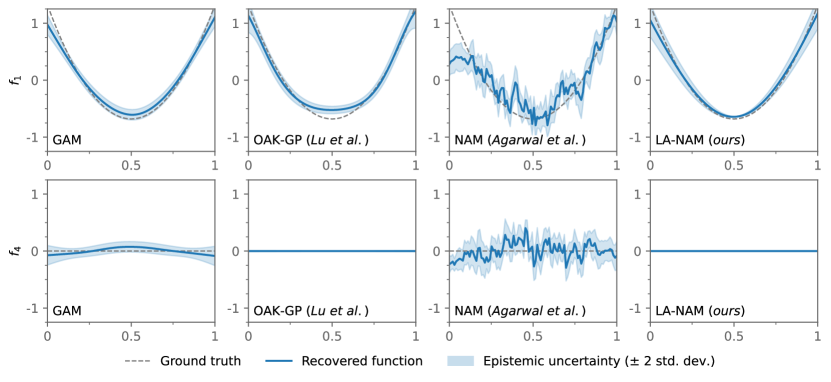
Figure 1: Regression on a synthetic dataset with known additive structure (see Section 4.1 and Section B.8 for details). The la-nam fits the data well, provides useful uncertainty estimates, and along with OAK-GP correctly ignores the uninformative feature ($f_{4}$, bottom.)

Over the past decade, deep neural networks (DNNs) have found successful applications in numerous fields, ranging from computer vision and speech recognition to natural language processing and recommendation systems. This success is often attributed to the growing availability of data in all areas of science and industry. However, the inherent complexity and lack of transparency of DNNs have impeded their use in domains where understanding the reasoning behind their decision-making process is important (Pumplun et al., 2021; Veale et al., 2018).

Model-agnostic methods, such as partial dependence (Friedman, 2001), SHAP (Lundberg & Lee, 2017), and LIME (Ribeiro et al., 2016), provide a standardized approach to explaining predictions in machine learning, but the explanations they generate for DNNs are not faithful representations of their full complexity (Rudin, 2019). Instead, one can enhance transparency in DNNs by acting directly on the architecture and training procedure. For instance, in generalized additive models (Hastie & Tibshirani, 1999), the response variable $y$ is associated with inputs $x_{1}$, …, $x_{p}$ using an additive structure of the form

$$g(\mathop{\mathbb{E}}[y\,|\,x_{1},\,\dots,\,x_{p}])=\beta_{0}+f_{1}(x_{1})+\dots+f_{p}(x_{p}).$$ (1)

The neural additive models (NAMs) introduced by Agarwal et al. (2021) hinge on this concept. In this model architecture, each input dimension is processed by a distinct sub-network, elucidating the connections between the input features and the model’s predictions. However, restricting neural network models in this way can lead to overconfidence, overreliance on uninformative features and obliviousness to underlying feature interactions.

Main contributions.

In this work, we (a) propose a Bayesian variant of the NAM by deriving a tailored linearized Laplace inference (MacKay, 1994) on the subnetworks. We show that this improves intelligibility by encouraging smoothness and enhancing uncertainty estimation. Moreover, (b) this model construction enables the estimation of the marginal likelihood, which serves as a Bayesian model selection criterion. This enables us to mitigate the impact of uninformative features, further contributing to the robustness and trustworthiness of the model. Also, (c) in situations where strong feature interactions exist in the ground-truth function and cause poor performance of first-order additive models, we leverage our Laplace approximation to automatically select informative feature interactions, which can then be added to the model to improve its overall performance. Finally, (d) we show on tabular regression and classifications benchmarks, as well as on challenging real-world medical tasks, that our proposed la-nam performs competitively with the baselines while offering more interpretable global and local explanations.

2 Related Work

Neural additive models.

Several constructions have been proposed for the generalized additive models (GAMs) of Hastie & Tibshirani (1999), using both smoothing splines (Wahba, 1983) and gradient-boosted decision trees (Friedman, 2001; Lou et al., 2012, 2013). Neural networks are also particularly compelling candidates for the construction of GAMs since they can be made to approximate continuous functions up to arbitrary precision given sufficient complexity (Cybenko, 1989; Maiorov & Pinkus, 1999; Lu et al., 2017). The neural additive model (NAM) proposed by Agarwal et al. (2021) is constructed using ensembles of feed-forward networks. In order to fit jagged functions and promote diversity for ensembling, the authors propose the exponential unit (ExU) activation in which weights are learned in logarithmic space. The GAMI-Net proposed around the same time by Yang et al. (2021) is closely related but single networks are used in place of an ensemble, and the model also supports learning of feature interaction terms. Recently proposed extensions to NAMs include feature selection through sparse regularization of the networks (Xu et al., 2022), generation of confidence intervals using spline basis expansion (Luber et al., 2023), and estimation of the skewness, heteroscedasticity, and kurtosis of the underlying data distributions (Thielmann et al., 2023). Our work extends NAMs via Laplace-approximated Bayesian inference to endow them with principled uncertainty estimation and feature interaction and selection abilities within a unified Bayesian framework.

Bayesian neural networks.

Bayesian neural networks promise to marry the expressivity of neural networks with the principled statistical properties of Bayesian inference (MacKay, 1992; Neal, 1993). There are many approximate inference techniques, such as Laplace inference (MacKay, 1992; Daxberger et al., 2021b), stochastic weight averaging (Maddox et al., 2019), dropout (Gal & Ghahramani, 2016), variational inference (e.g., Graves, 2011; Blundell et al., 2015; Khan et al., 2018), ensemble-based methods (Lakshminarayanan et al., 2017; Wang et al., 2019; D’Angelo & Fortuin, 2021), and sampling approaches (e.g., Neal, 1993; Neal et al., 2011; Welling & Teh, 2011). In our work, we leverage linearized Laplace (MacKay, 1994; Khan et al., 2019; Foong et al., 2019; Immer et al., 2021b) for inference in Bayesian NAMs. This is motivated by the Laplace approximation’s ability to provide reliable predictive uncertainties and marginal likelihood estimates, the latter of which is not readily available in most other approximations. Here, we devise a Laplace approximation that is specifically optimized for the structure of NAMs.

Additive Gaussian processes.

Gaussian Processes (GPs) are a powerful and flexible class of probabilistic models. GPs are also compelling for the construction of GAMs as they are characterized by their ability to model complex relationships, providing uncertainty estimates along with their predictions. Additive GPs have been explored in studies by Kaufman & Sain (2010), Duvenaud et al. (2011), Timonen et al. (2021) and Lu et al. (2022). Specifically, the Orthogonal Additive Kernel (OAK) proposed by Lu et al. (2022) enables both selection of features and feature interaction of all orders relying on the efficient computational scheme of Duvenaud et al. (2011) and the orthogonality constraint of Durrande et al. (2012). Our work equips NAMs with similar features through Bayesian inference.

Refer to Appendix C for further treatment of related work.

3 Laplace-Approximated NAM

We introduce a Bayesian formulation of neural additive models and propose a tractable inference procedure, which is based on the linearized Laplace approximation of neural networks (MacKay, 1991; Khan et al., 2019). The proposed model (la-nam) relies on a block-diagonal variant of the Gauss-Newton approximation with Kronecker factorization (Martens & Grosse, 2015) and uses the associated predictive and log-marginal likelihood (Immer et al., 2021a, b) to estimate feature-wise uncertainty and automatically select features. Further, we identify promising feature interactions by mutual information within the posterior.

3.1 Bayesian Neural Additive Model

We consider supervised learning tasks with inputs $\mathbf{x}_{n}\in\mathbb{R}^{D}$ and outputs $y_{n}$ where $y_{n}\in\mathbb{R}$ in regression and $y_{n}\in\{0,1\}$ in classification, and denote $\mathcal{D}=\{(\mathbf{x}_{n},y_{n})\}_{n=1}^{N}$ as the training set containing $N$ sample pairs. A neural additive model is a neural network $f$ consisting of sub-networks $f_{1},\dots,f_{D}$ with parameters $\boldsymbol{\theta}=\{\boldsymbol{\theta}_{1},\dots,\boldsymbol{\theta}_{D}$}, wherein each sub-network applies to an individual input dimension,

$$f(\mathbf{x};\,\boldsymbol{\theta})=f_{1}(x_{1};\,\boldsymbol{\theta}_{1})+\dots+f_{D}(x_{D};\,\boldsymbol{\theta}_{D}).$$ (2)

We refer to the sub-networks $f_{d}:\mathbb{R}\times\mathbb{R}^{P}\to\mathbb{R}$, with parameters $\boldsymbol{\theta}_{d}\in\mathbb{R}^{P}$, as feature networks. For simplicity, we assume that all feature networks share the same architecture. In practice, it can vary to accommmodate mixed feature types such as binary or categorical features. The sum is mapped to an output $y$ using a likelihood function $p(\mathcal{D}\,|\,\boldsymbol{\theta}_{1},\dots,\boldsymbol{\theta}_{D})$ with inverse link function $g^{-1}(\,\cdot\,)$, e.g., the sigmoid for classification, such that we have $\mathop{\mathbb{E}}[y\,|\,\mathbf{x}]=g^{-1}(f(\mathbf{x}))$, and

$$p(\mathcal{D}\,|\,\boldsymbol{\theta})=\prod_{n=1}^{N}p(y_{n}\,|\,f(\mathbf{x}_{n};\,\boldsymbol{\theta})).$$ (3)

We impose a zero-mean Gaussian prior distribution over the parameters of each feature network with prior precision hyperparameters $\boldsymbol{\lambda}=\{\lambda_{1},\dots,\lambda_{D}\}$,

$$p(\boldsymbol{\theta})=p(\boldsymbol{\theta}_{1},\dots,\boldsymbol{\theta}_{D}\,|\,\boldsymbol{\lambda})=\prod_{d=1}^{D}\mathcal{N}(\boldsymbol{\theta}_{d};\,\mathbf{0},\,\lambda_{d}^{-1}\mathbf{I}).$$ (4)

These terms adaptively regularize the network parameters and enable feature selection in a similar fashion to automatic relevance determination (ARD; MacKay, 1994; Neal, 1995). Large values push the corresponding feature networks toward zero and low values encourage highly non-linear fits. In practice, one can also use separate priors and precision terms for each layer of each feature network, as this has been shown to be beneficial in linearized Laplace (Immer et al., 2021a; Antorán et al., 2022).

3.2 Linearized Laplace Approximation

We devise a linearized Laplace approximation of the Bayesian NAM to obtain predictive uncertainties and select features as well as their interactions within a single framework, which we call la-nam. The posterior predictive of the linearized Laplace is well-established and known to provide calibrated uncertainty estimates (Daxberger et al., 2021a). Further, its marginal likelihood estimates are useful to perform automatic relevance determination of feature networks during training and optimize observation noise parameters (MacKay, 1994). Lastly, we use the mutual information in the posterior between feature network pairs to identify promising feature interactions.

We linearize the model around a parameter estimate $\boldsymbol{\theta}^{*}$,

$$f^{\mathrm{lin}}(\mathbf{x};\,\boldsymbol{\theta}^{*}) =f^{\mathrm{lin}}_{1}(x_{1};\,\boldsymbol{\theta}_{1}^{*})+\dots+f^{\mathrm{lin}}_{D}(x_{D};\,\boldsymbol{\theta}_{D}^{*}),$$ (5)

$$f^{\mathrm{lin}}_{d}(x_{d};\,\boldsymbol{\theta}_{d}^{*}) =f_{d}(x_{d};\,\boldsymbol{\theta}_{d}^{*})+\mathcal{J}_{\boldsymbol{\theta}^{*}}^{(d)}(x_{d})(\boldsymbol{\theta}_{d}-\boldsymbol{\theta}_{d}^{*}),$$ (6)

where $\mathcal{J}_{\boldsymbol{\theta}}^{(d)}:\mathbb{R}\to\mathbb{R}^{P}$ is the Jacobian of the $d$-th feature network w.r.t. $\boldsymbol{\theta}_{d}$, such that $[\mathcal{J}_{\boldsymbol{\theta}}^{(d)}]_{i}=\partial f_{d}/\partial\theta_{d,i}$. This step follows from the linearity of the gradient operator and the fact that $\partial f_{d}/\partial\theta_{d^{\prime}\!\!,\,i}=0$ for $d\neq d^{\prime}$.

This reduces the model to a generalized linear model in the Jacobians whose posterior can be approximated with a block-diagonal Laplace approximation as

$$q(\boldsymbol{\theta})=\mathcal{N}(\boldsymbol{\theta}^{*},\,\boldsymbol{\Sigma}^{*}),\quad\boldsymbol{\Sigma}^{*}\approx\begin{bmatrix}\boldsymbol{\Sigma}_{1}&\dots&0\\ \vdots&\ddots&\vdots\\ 0&\dots&\boldsymbol{\Sigma}_{D}\\ \end{bmatrix}\!\!,$$ (7)

where the diagonal covariance blocks are determined using the feature network Jacobians and second derivatives of the log-likelihood, $\gamma_{n}=-\frac{\partial^{2}}{\partial f^{2}}\log p(y_{n}\,|\,f_{n})$, by

$$\boldsymbol{\Sigma}_{d}=\left[\left[\sum_{n=1}^{N}\gamma_{n}\cdot\mathcal{J}_{\boldsymbol{\theta}^{*}}^{(d)}(x_{n,d})^{\top}\mathcal{J}_{\boldsymbol{\theta}^{*}}^{(d)}(x_{n,d})\right]+\lambda_{d}\mathbf{I}\right]^{-1}\!\!\!\!\!\!\!\!.$$ (8)

The approximation also leads to an additive structure over feature networks in the log-marginal likelihood,

$$\log p(\mathcal{D}\,|\,\boldsymbol{\lambda}) \approx\log p(\mathcal{D},\boldsymbol{\theta}^{*}\,|\,\boldsymbol{\lambda})-\tfrac{1}{2}\log|\tfrac{1}{2\pi}\boldsymbol{\Sigma}|$$ (9)

$$\geq\log p(\mathcal{D},\boldsymbol{\theta}^{*}\,|\,\boldsymbol{\lambda})-\tfrac{1}{2}{\textstyle\sum_{d}\log|\tfrac{1}{2\pi}\boldsymbol{\Sigma}_{d}|}$$ (10)

where the lower bound is a consequence of the block-diagonal structure (Immer et al., 2023).

In practice, we further approximate the covariance blocks $\boldsymbol{\Sigma}_{d}$ by using layer-wise Kronecker factorization (Ritter et al., 2018; Daxberger et al., 2021b), thereby avoiding the memory and computational complexity associated with the quadratic size in the number of parameters $P$.

3.2.1 Feature Network Selection

During training, the feature networks are implicitly compared and selected using adaptive regularization. This selection mechanism arises from the optimization of the lower bound on the Laplace approximation to the log-marginal likelihood in Equation 10, which we denote here as $\log q(\mathcal{D}\,|\,\boldsymbol{\lambda})$. In the automatic relevance determination (ARD) procedure of MacKay (1994) and Neal (1995), parameters of the first layer are grouped together according to their input feature and regularized as one. In our case, one feature network corresponds to one group.

We maximize the lower bound on the log-marginal likelihood, $\max_{\boldsymbol{\lambda}}\log q(\mathcal{D}\,|\,\boldsymbol{\lambda})$, by taking gradient-based updates during training with

$$\tfrac{\partial}{\partial\lambda_{d}}\log q(\mathcal{D}\,|\,\boldsymbol{\lambda})=\tfrac{P}{\lambda_{d}}-||\boldsymbol{\theta}_{d}^{*}||_{2}^{2}-\operatorname{Tr}\boldsymbol{\Sigma}_{d}.$$ (11)

An intuition of the corresponding closed-form update derived by MacKay (1991) is given in Tipping (2001): the optimal value of $\lambda_{d}$ is a measure of the concentration of $\boldsymbol{\Sigma}_{d}$ relative to the prior and depends on how well the data determines the parameters $\boldsymbol{\theta}_{d}$. Large values of $\lambda_{d}$ lead to strong regularization and effectively switch off the $d$-th feature network. This is depicted in Figure 1, where our method demonstrates its ability to disregard an uninformative feature. As a result, the procedure can lead to enhanced model interpretability and robustness as it redirects the attention to smaller subsets of informative features.

3.2.2 Feature Network Predictive

Due to linearization, we can obtain function-space predictive uncertainties in a closed form like for Gaussian processes. Given an unobserved sample $\mathbf{x}^{*}$, the predictive variance of the linearized model $f^{\mathrm{lin},\,*}$ corresponds to the sum of predictive variances of the linearized feature networks,

$$\mathop{\mathbb{V}}[f^{\mathrm{lin},\,*}\,|\,\mathbf{x}^{*}] ={\textstyle\sum_{d}\mathop{\mathbb{V}}[f_{d}^{\mathrm{lin},\,*}\,|\,x_{d}^{*}]}$$ (12)

$$={\textstyle\sum_{d}\mathcal{J}_{\theta^{*}}^{(d)}(x_{d}^{*})^{\top}\boldsymbol{\Sigma}_{d}\mathcal{J}_{\theta^{*}}^{(d)}(x_{d}^{*}).}$$ (13)

This is due to the block-diagonal structure of our posterior approximation in Equation 7. We discuss further properties and advantages of this in Section A.1.

As training progresses, the feature networks may shift to satisfy a global intercept value in their sum. They should therefore be shifted back around zero before visualization by removing the expected contribution,

$$\textstyle\hat{f}_{d}(x_{d}^{*})=f_{d}(x_{d}^{*})-\mathop{\mathbb{E}}_{\mathbf{x}\sim p(\mathcal{D})}[f_{d}(x_{d})].$$ (14)

Importantly, this adjustment does not affect the predictive variance $\mathop{\mathbb{V}}[f_{d}^{\mathrm{lin},\,\ast}]$. This variance estimate can be used to generate credible intervals for local and global explanations of the model, as shown in Figure 2 and 4. Notably, this allows the model to not only communicate on which data points it is uncertain, but also which features are responsible for the predictive uncertainty. Also, refer to Figure 1 for an example of the obtained predictive uncertainties.

Table 1: Negative test $\log$-likelihood (lower is better) on the UCI regression (top) and classification (bottom) benchmarks. Results better or within one standard error of the best performance of first-order methods in the first block are in bold. Results in green indicate an improvement beyond one standard error when compared to the corresponding model without second-order interactions. The la-nam performs competitively with the other additive models and often outperforms the nam. Moreover, when 10 interactions are selected, it almost always improves and often reaches competitive performance with the fully-interacting LightGBM.

Dataset nam la-nam oak-gp la-nam₁₀ oak-gp_* LightGBM autompg ($n$ = 392) 2.69 ±0.16 2.46 ±0.08 2.55 ±0.10 2.45 ±0.09 2.46 ±0.14 2.53 ±0.07 concrete ($n$ = 1030) 3.46 ±0.12 3.25 ±0.03 3.19 ±0.09 3.18 ±0.04 2.81 ±0.06 3.09 ±0.09 energy ($n$ = 768) 1.48 ±0.02 1.44 ±0.02 1.46 ±0.02 1.11 ±0.12 0.61 ±0.04 0.81 ±0.05 kin8nm ($n$ = 8192) -0.18 ±0.01 -0.20 ±0.00 0.09 ±0.01 -0.28 ±0.02 0.09 ±0.01 -0.50 ±0.03 naval ($n$ = 11934) -3.87 ±0.01 -7.24 ±0.01 -8.93 ±0.07 -7.44 ±0.07 -9.43 ±0.01 -5.19 ±0.01 power ($n$ = 9568) 2.89 ±0.02 2.85 ±0.01 2.81 ±0.03 2.79 ±0.01 2.73 ±0.02 2.67 ±0.02 protein ($n$ = 45730) 3.02 ±0.00 3.02 ±0.00 3.00 ±0.00 2.94 ±0.01 2.88 ±0.00 2.83 ±0.00 wine ($n$ = 1599) 1.02 ±0.04 0.98 ±0.03 1.14 ±0.04 0.97 ±0.03 1.67 ±0.65 0.96 ±0.03 yacht ($n$ = 308) 2.24 ±0.08 1.81 ±0.10 1.86 ±0.11 0.76 ±0.20 0.79 ±0.17 1.37 ±0.28 australian ($n$ = 690) 0.38 ±0.04 0.34 ±0.03 0.33 ±0.03 0.34 ±0.03 0.35 ±0.03 0.31 ±0.03 breast ($n$ = 569) 0.16 ±0.03 0.10 ±0.02 0.07 ±0.01 0.10 ±0.02 0.09 ±0.01 0.09 ±0.01 heart ($n$ = 270) 0.41 ±0.04 0.33 ±0.02 0.42 ±0.06 0.33 ±0.03 0.42 ±0.06 0.39 ±0.04 ionosphere ($n$ = 351) 0.31 ±0.04 0.25 ±0.04 0.22 ±0.02 0.27 ±0.03 0.21 ±0.03 0.19 ±0.03 parkinsons ($n$ = 195) 0.29 ±0.04 0.26 ±0.03 0.27 ±0.03 0.25 ±0.03 0.21 ±0.02 0.22 ±0.03

3.2.3 Feature Network Interaction

Many datasets are not truly additive and thus require modeling interactions of features to adequately fit the data. However, it is a priori unclear which features exhibit underlying interactions. As the search space grows exponentially for higher-order interactions, we focus here on the second order. In second-order feature interaction detection, the goal is to find a subset of all existing $D^{2}$ interaction pairs that, when added to the model, maximize the gain in performance. For each selected interacting pair $(d,\,d^{\prime})$, we can then append a joint feature network $f_{d,\,d^{\prime}}(x_{d},\,x_{d^{\prime}})$ and perform fine-tuning of the model with the appended networks as part of a secondary training stage.

Our method for detecting and selecting second-order interactions makes use of the mutual information between feature networks. If the mutual information between the feature network parameters $\boldsymbol{\theta}_{d}$ and $\boldsymbol{\theta}_{d^{\prime}}$ is high, then conditioning on the values of either of these should provide information about the other and thus, their functions. This can be an indication that a joint feature network for this pair may improve the data fit.

Although the mutual information between feature networks is zero in the approximation of Equation 7, this is not necessarily the case in the true posterior. For the purpose of determining mutual information of the feature networks, we therefore fit separate last-layer Laplace approximations of the model for all feature pairs. After the first training stage, we consider only the scalar output multiplier weights $\theta_{d}$ of each feature network and for each candidate pair of features $(d,\,d^{\prime})$ determine the scalar marginal variances $\sigma_{d}^{2}$, $\sigma_{d^{\prime}}^{2}$, and co-variance $\sigma_{d,d^{\prime}}^{2}$ in the resulting $D\times D$ posterior covariance matrix and is thus computationally efficient. The mutual information can then be approximated using

$$\mathrm{I}(\theta_{d};\,\theta_{d^{\prime}}) =\mathrm{H}(\theta_{d})+\mathrm{H}(\theta_{d^{\prime}})-\mathrm{H}(\theta_{d},\,\theta_{d^{\prime}})$$ (15)

$$\approx\tfrac{1}{2}\log\left[\sigma_{d}^{2}\sigma_{d^{\prime}}^{2}(\sigma_{d}^{2}\sigma_{d^{\prime}}^{2}-\sigma_{d,d^{\prime}}^{2})^{-1}\right]$$ (16)

$$=\tfrac{1}{2}\log\left[1-\mathrm{Corr}(\theta_{d},\,\theta_{d^{\prime}})^{2}\right]^{-1}.$$ (17)

Finally, we select interactions by computing the mutual information for all feature pairs and taking the top-$k$ highest scoring pairs. Importantly, this can be done after training in the first stage and without the need for an additional model to assess interaction strength. We show in the experiments that with only a few second-order interactions selected this way the performance of the additive model can improve to be at the level of a fully-interacting baseline.

4 Experiments

We evaluate the proposed la-nam on a collection of synthetic and real-world datasets emphasizing its potential for supporting decision-making in the medical field. To assess performance, we compare against the original nam of Agarwal et al. (2021) and other generalized additive models, namely, a smoothing spline generalized additive model (gam), with smoothing parameters selected via cross-validation (Hastie & Tibshirani, 1999; Servén et al., 2018), and a GP with an orthogonal additive kernel (oak-gp; Lu et al., 2022). We also include LightGBM (Ke et al., 2017) as a state-of-the-art fully-interacting model which approximates the maximal attainable performance in tabular regression and classification tasks (Grinsztajn et al., 2022). Detailed information regarding the experimental setup is provided in Section B.7.

Table 2: Comparison of model performance on ICU mortality prediction tasks. Mean and standard error reported with five seeds. AUROC and AUPRC are in percent. Bold indicates best performance first-order methods; green/ red highlights an improvement/decrease with interactions. The oak-gp runs out of memory for HiRID due to the number of features. The la-nam generally outperforms the nam, and improves with 10 interacting features on MIMIC-III, becoming competitive with the fully-interacting LightGBM gold-standard.

Task MIMIC-III ICU Mortality HiRID ICU Mortality Metric AUROC ($\uparrow$) AUPRC ($\uparrow$) NLL ($\downarrow$) AUROC ($\uparrow$) AUPRC ($\uparrow$) NLL ($\downarrow$) nam 77.6 ± 0.03 32.3 ± 0.03 0.274 ± 8e-5 89.6 ± 0.17 60.7 ± 0.14 0.228 ± 1e-2 la-nam 79.6 ± 0.01 34.8 ± 0.04 0.264 ± 5e-5 90.1 ± 0.03 60.5 ± 0.14 0.174 ± 2e-4 oak-gp 79.9 ± 0.03 35.2 ± 0.11 0.263 ± 1e-4 — — — la-nam₁₀ 80.2 ± 0.10 35.2 ± 0.06 0.262 ± 3e-4 90.1 ± 0.01 60.5 ± 0.20 0.174 ± 4e-4 oak-gp_* 71.7 ± 0.66 28.5 ± 0.42 0.288 ± 1e-3 — — — LightGBM 80.6 ± 0.08 35.6 ± 0.19 0.261 ± 3e-4 90.7 ± 0.00 61.6 ± 0.00 0.172 ± 0.00

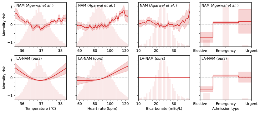
Figure 2: Risk of mortality and associated epistemic uncertainty ($\pm$ 2 std. deviations) on the MIMIC-III mortality prediction task. The la-nam relies on smoother feature curves and provides useful uncertainties while ignoring the uninformative feature.

The nam lacks a built-in notion of epistemic uncertainty. As such, figures which provide the uncertainty associated with its predictions use the standard deviation of the recovered functions across the deep ensemble of feature networks.

4.1 Illustrative Example

To demonstrate the capability of recovering purely additive structures from noisy data, we constructed a synthetic regression dataset for which the true additive functions are known. Generalized additive models are expected to accurately recover the additive functions present in this dataset since it is designed in such a way that there is no interaction between the input features.

In Figure 1, we show the recovered functions for $f_{1}$ and $f_{4}$ along with the ground-truth quadratic function $f_{1}$ and zero function $f_{4}$. The nam exhibits pronounced jumpy behavior due to the presence of noise, resulting in a considerably poor mean fit. In contrast, the proposed la-nam fits the data accurately while maintaining a good estimate of epistemic uncertainty. It is less susceptible to misattributing noise to the recovered functions compared to the nam. This is particularly striking for the uninformative function $f_{4}$, since only the la-nam and oak-gp correctly identify that it should have no effect through their Bayesian model selection. More details and visualizations are in Section B.8

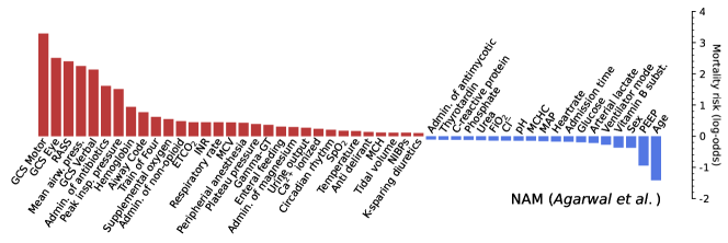
Figure 3: Local explanations for the risk of a sample patient in the HiRID mortality task in the nam. Features which contribute less than 0.1 to the log-odds magnitude are omitted. The NAM selects a large number of features and does not provide uncertainty estimates.

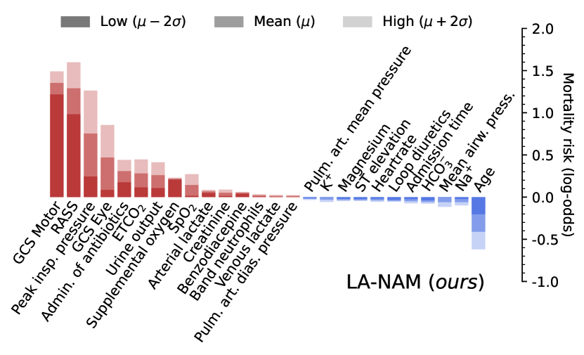
Figure 4: Local explanations from the la-nam for the same patient of Figure 3. Features whose credible intervals overlap with zero are omitted. The model selects far fewer features and provides uncertainty estimates, further aiding interpretation.

4.2 UCI Regression and Classification

We benchmark the la-nam and baselines on the standard selection of UCI regression and binary classification datasets. Each dataset is split into five cross-validation folds and the mean and standard error of model performance are reported across folds. We split off 12.5% of the training data as validation data for the nam. This extra validation data is not required for the la-nam, since it is tuned using the estimated $\log$-marginal likelihood. Additionally, both the la-nam and oak-gp have support for selecting and fitting second-order feature interactions, further enhancing their modeling capacity. For these models, we also present results where we have enabled feature interactions: We identify and fine-tune the top-10 feature pairs of the la-nam (which we denote as la-nam₁₀), and increase the oak-gp’s maximum interaction depth to 2 so that it models all pairwise interactions (denoted as oak-gp_*).

In Table 1, we report the negative $\log$-likelihood averaged over test samples. The nam does not provide an estimate of the observation noise in regression, so it is assigned a maximum likelihood fit using its training data. The la-nam consistently demonstrates competitive performance across multiple datasets. It tends to exhibit lower average negative $\log$-likelihood, indicating better performance, compared to the nam and performs comparatively well versus the oak-gp. la-nam₁₀, which refers to the fined-tuned model with top-10 feature interactions, almost always improves performance on regression when compared to its non-feature-interactive counterpart and often reaches the performance of the fully-interacting LightGBM. Note that this might also be related to its ability to ignore uninformative features, which has been identified as a main weakness of neural networks on tabular data compared to tree-based methods (Grinsztajn et al., 2022). A wider set of models along with additional performance and calibration metrics is considered in Sections B.6 and B.5.

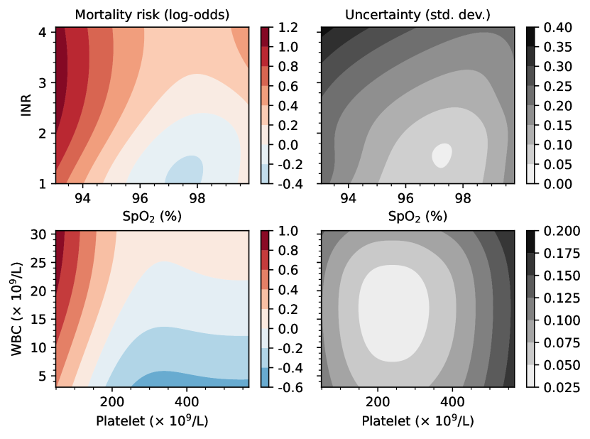
Figure 5: Feature interactions uncovered in the MIMIC-III dataset by the la-nam. (left) Last-layer posterior correlation matrix, used to select the most informative feature interaction pairs. (right) Two selected example feature interactions and associated uncertainty.

4.3 Intensive Care Unit Mortality Prediction

To gain insights into the behavior of our method within a real-world clinical context, we investigate its performance in predicting patient mortality based on vital signs recorded 24 hours after admission into an intensive care unit (ICU). To accomplish this, we utilize the MIMIC-III database (Johnson et al., 2016) and employ the pre-processing outlined by Lengerich et al. (2022). Additionally, we leverage the HiRID database (Faltys et al., 2021) and adopt the pre-processing methodology presented by Yèche et al. (2021). Notably, our objective extends beyond achieving competitive predictive performance: we aim to provide valuable insights into the underlying sources of risk within the ICU to facilitate a clearer understanding of critical care dynamics.

Predictive performance.

Table 2 presents a summary of the test performance achieved by the various methods. For the MIMIC-III dataset, a total of 14,960 patients were considered, with 2,231 held out as the test set. Similarly, the HiRID dataset comprises 27,347 patients, with 8,189 held out for testing purposes. On these tasks, the la-nam demonstrates superior performance compared to the nam in the key evaluation metrics of area under the ROC and precision-recall curve (AUROC and AUPRC), as well as average negative $\log$-likelihood (NLL). Figure 2 showcases a subset of the recovered additive structure from the MIMIC-III dataset. In each subplot, the background displays a histogram depicting the distribution of feature values. Note that the nam exhibits the same jumpy behavior observed in the synthetic example, adversely affecting interpretability, while the la-nam yields smoother curves, due to its optimized Bayesian prior. We find that the identified relationships of the displayed variables and risk by la-nam appear consistent with medical knowledge (personal communication with medical experts). We also find that the la-nam effectively captures and quantifies epistemic uncertainty, aligning with the presence or absence of sufficient samples.

Feature selection.

This experiment also illustrates the ability of the la-nam to assess the relevance of features through the selection of feature networks. Because of their linear dependency, both high bicarbonate levels and low anion gap are indicators of metabolic acidosis (Kraut & Madias, 2010). The la-nam determines that the risk associated with bicarbonate can be adequately captured using only the measurement of the anion gap. Consequently, as demonstrated in Figure 2, it entirely disregards the bicarbonate feature. See Section B.2 for an ablation experiment confirming this.

Interpretability.

The epistemic uncertainty and feature-selecting property of the la-nam play significant roles in the effectiveness of the generated local explanations. This advantage is clear in Figures 3 and 4, where we compare the breakdown of risk factors between the nam and la-nam, respectively. We show that the la-nam selects a noticeably condensed, more concise set of features. Moreover, it provides uncertainties in local explanations, bringing valuable insight by acknowledging the inherent variability and potential limitations of the model. In this case, it allows clinicians to gauge the reliability and robustness of the predicted risk factors, enabling more informed decision-making and facilitating trust in the model’s outputs.

Feature interactions.

In addition to the first-order models, both the la-nam and oak-gp were evaluated with feature interactions (la-nam₁₀ and oak-gp_* in Table 2). Incorporating these interactions led to significantly improved performance for the la-nam₁₀ on the MIMIC-III dataset, reaching competitive performance with the fully-interacting LightGBM gold standard. On the left side of Figure 5, the last-layer correlation matrix for second-order interactions is presented, revealing the relationships between the different feature pair candidates for inclusion in the second-order fine-tuning stage. On the right side, specific interactions involving the risk factors of WBC and Platelet, as well as INR and SpO₂, are depicted. In particular, we show an increase in mortality risk for high white blood cell and low platelet counts as well as for elevated INR and low oxygen saturation. While the first interaction is characteristic of immune thrombocytopenia (Cooper & Ghanima, 2019), a known risk factor for critically ill patients (Baughman et al., 1993; Trehel-Tursis et al., 2012), the second has not been studied in the literature. Hence, by enabling second-order interaction selection, la-nam may also help to discover new risk factors (of course, follow-up studies would be needed).

5 Conclusion

In this work, we have introduced a Bayesian adaptation of the widely used neural additive model and derived a customized linearized Laplace approximation for inference. This approach allows for a natural decomposition of epistemic uncertainty across additive subnetworks, as well as implicit feature selection by optimizing the $\log$-marginal likelihood. Our empirical results illustrate the robustness of our Laplace-approximated neural additive model (la-nam) against noise and uninformative features. Furthermore, when allowed to autonomously select its feature interactions, the la-nam demonstrates performance on par with fully interacting gold-standard baselines. The la-nam thus emerges as a viable option for applications with safety considerations and as a tool for data-driven scientific discovery. Moreover, our work underscores the potential for future research at the intersection of interpretable machine learning and Bayesian inference. Overall, this work contributes to the vision of powerful, robust, yet transparent and understandable machine learning models. We hope that our work will inspire further advances in Bayesian additive models, marrying transparency with probabilistic modeling.

Impact Statement

Since this is basic research, we do not foresee any immediate broader impact. However, as the proposed model can lend itself well to medical tasks (see Section 4.3), it could have an impact on improving medical care. These features may also have relevance in other critical domains where the use of non-transparent models can be problematic, such as jurisdiction, hiring, or finance.

Additionally, in applications where fairness and implicit biases are important considerations, detecting biases or potential lack of fairness could be facilitated by the feature-independence property and the feature-selecting capabilities of our model. However, it should be noted that existing biases in the data will likely propagate to the model, so this should be critically assessed.

Acknowledgments

We thank Ben Lengerich for providing us the pre-processed MIMIC-III dataset used in the paper.

This project was supported by grant #2022-278 of the Strategic Focus Area “Personalized Health and Related Technologies (PHRT)” of the ETH Domain. A. I. acknowledges funding by the Max Planck ETH Center for Learning Systems (CLS). V. F. was supported by a Branco Weiss Fellowship.

Appendix A Additional Theoretical Results and Discussion

In this section, we provide additional details on the derivation of our approximate posterior for Bayesian NAMs and discuss in further detail the interaction detection procedure and theoretical computational bounds.

A.1 Feature Network Independence

The approximate posterior defined in Equation 7 results in feature networks that are mutually independent due to the block-diagonal structure of the covariance matrix. This independence is needed for the decomposition of the predictive variance in Equation 12. We elaborate here on the motivation behind this independence assumption.

As a thought experiment, suppose we wanted to find estimates of two variable terms $b_{1}$ and $b_{2}$, such that their sum is equal to some constant $C$. We also desire that neither term $b_{1}$ or $b_{2}$ dominate the other so that they are roughly equally balanced. One possible setup for finding a maximum a posteriori (MAP) estimate of $b_{1}$ and $b_{2}$ could be to design a cost function $L(b_{1},\,b_{2})$ where the MAP solution is a minimizer,

$$p(b_{1},\,b_{2})=\mathcal{N}([b_{1},\,b_{2}]^{\top};\,\mathbf{0},\,\lambda^{-1}\mathbf{I}),\quad p(C\,|\,b_{1},\,b_{2})=\mathcal{N}(C;\,b_{1}+b_{2},\,1),$$ (A.1)

$$\log p(b_{1},\,b_{2}\,|\,C) \propto\log p(C\,|\,b_{1},\,b_{2})+\log p(b_{1},\,b_{2})$$ (A.2)

$$\propto-(b_{1}+b_{2}-C)^{2}-\lambda(b_{1}^{2}+b_{2}^{2})\quad\overset{\mathrm{def}}{=}-L(b_{1},\,b_{2}).$$ (A.3)

For illustrative purposes, we set $C=20$ and $\lambda=0.01$. In the left side of Figure A.1, we visualize the cost function values $L(b_{1},\,b_{2})$ and highlight the MAP solution as a white cross. Now, suppose we are interested in finding an approximate posterior distribution for $b_{1}$ and $b_{2}$ with a Laplace approximation centered at the MAP estimate. When we treat $b_{1}$ and $b_{2}$ as jointly dependent variables, we obtain the Gaussian approximate posterior distribution depicted on the right side of Figure A.1.

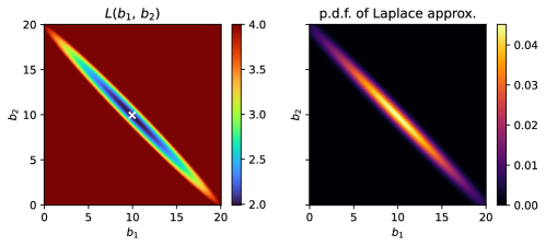
Figure A.1: Laplace approximation of the illustrative example in Section A.1. ($C=20$, $\lambda=0.01$)

In this approximation, $b_{1}$ and $b_{2}$ exhibit strong anti-correlation. This can be attributed to the observation that adjusting $b_{1}$ by some amount $\Delta$ can be accounted for by adjusting $b_{2}$ by $-\Delta$, since $b_{1}+b_{2}=(b_{1}+\Delta)+(b_{2}-\Delta)$. Within the realm of Bayesian NAMs, this property is considered undesirable. Ideally, we want the credible intervals for a feature network $f_{d}$ to solely reflect changes in its shape, without being influenced by vertical translations of other feature networks. To circumvent the scenario illustrated above, one can adopt a strategy where $b_{1}$ and $b_{2}$ are treated as independent variables. This involves performing a first Laplace approximation for $b_{1}$ while keeping $b_{2}$ fixed, followed by a separate Laplace approximation for $b_{2}$ keeping $b_{1}$ fixed. In our model, this is ensured by performing separate Laplace approximations for each feature network.

Nonetheless, the true posterior may contain strong statistical dependency across the feature networks. Therefore, for feature pairs which demonstrate high mutual information (Section A.2.1) or exhibit significant improvement on the marginal likelihood bound (Section A.2.2), we suggest to introduce second-order joint feature networks. The purpose of these networks is to explicitly capture these dependencies in the resulting fine-tuned model.

A.2 Feature Interaction Selection

In this section, we expand on the feature interaction selection based on the mutual information and also provide an alternative selection procedure which is phrased as model selection and optimization of the marginal likelihood.

A.2.1 Feature Interaction via Mutual Information

To select feature interactions, we consider the mutual information (MI) between the posteriors of feature networks. If the mutual information between ${\boldsymbol{\theta}}_{d}$ and ${\boldsymbol{\theta}}_{d^{\prime}}$ is high, it is simultaneously high between the functional posteriors $f_{d}$ and $f_{d^{\prime}}$. This means that conditioning on the output of feature network $f_{d}$ can provide information about the posterior of feature network $f_{d^{\prime}}$, and therefore be an indication that a joint feature network for the interacting features could ultimately improve the la-nam fit. In a separate dense covariance matrix Laplace approximation, each candidate pair $(d,d^{\prime})$ has two marginal posteriors and a joint posterior. These are Gaussian distributions with corresponding covariance matrices ${\boldsymbol{\Sigma}}_{d},{\boldsymbol{\Sigma}}_{d^{\prime}}$, and ${\boldsymbol{\Sigma}}_{d,\,d^{\prime}}$. The mutual information can be approximated using

$$\mathrm{I}({\boldsymbol{\theta}}_{d};\,{\boldsymbol{\theta}}_{d^{\prime}}) \approx-\mbox{$\frac{1}{2}$}\log|{\boldsymbol{\Sigma}}_{d,\,d^{\prime}}({\boldsymbol{\Sigma}}_{d}\oplus{\boldsymbol{\Sigma}}_{d^{\prime}})^{-1}|=-\mbox{$\frac{1}{2}$}\log[|{\boldsymbol{\Sigma}}_{d,\,d^{\prime}}||{\boldsymbol{\Sigma}}_{d}^{-1}||{\boldsymbol{\Sigma}}_{d^{\prime}}^{-1}|],$$ (A.4)

where $\oplus$ denotes block-diagonal concatenation. Constructing the full covariance matrix can be prohibitively expensive for a la-nam containing many feature networks. Instead, we can iteratively compute the covariance blocks $\boldsymbol{\Sigma}_{d,\,d^{\prime}}$ and determine the mutual information of each pair using Jacobians and precision matrices which are at most $2P\times 2P$ large (Daxberger et al., 2021c). Alternatively, we propose to use a last-layer approximation in Section 3.2.3 which turns the computation into $D\times D$ matrices and relies on scalar marginal variances.

For linearized Laplace approximations one can show that this is closely related to maximizing the mutual information of the posterior on $f_{d}$ and $f_{d^{\prime}}$ over the training set. In other words, how much information is gained about $f_{d}$ when observing $f_{d^{\prime}}$ and vice-versa. The joint posterior predictive on $f_{d}$ and $f_{d^{\prime}}$ is a Gaussian with a $2\times 2$ covariance matrix per data point, meaning $N\times N$ marginal predictive covariance matrices ${\mathbf{S}}_{d}$ and ${\mathbf{S}}_{d^{\prime}}$, and a $2N\times 2N$ joint predictive covariance matrix ${\mathbf{S}}_{d,\,d^{\prime}}$, when considering the entire training set. In similar fashion to Equation A.4, the mutual information of the functional posterior distribution can be determined by taking

$$\mathrm{I}({\mathbf{f}}_{d};\,{\mathbf{f}}_{d^{\prime}})=-\mbox{$\frac{1}{2}$}\log|{\mathbf{S}}_{d,\,d^{\prime}}({\mathbf{S}}_{d}\oplus{\mathbf{S}}_{d^{\prime}})^{-1}|=-\mbox{$\frac{1}{2}$}\log[|{\mathbf{S}}_{d,\,d^{\prime}}||{\mathbf{S}}_{d}^{-1}|{\mathbf{S}}_{d^{\prime}}^{-1}|].$$ (A.5)

Moreover, taking ${\mathbf{J}}_{d,\,d^{\prime}}\in\mathbb{R}^{2N\times 2P}$ as the Jacobian matrix of $[f_{d},\,f_{d^{\prime}}]^{\mathrm{\textsf{\tiny T}}}$ with respect to $[\boldsymbol{\theta}_{d},\,\boldsymbol{\theta}_{d^{\prime}}]^{\mathrm{\textsf{\tiny T}}}$ over the training data, with brackets denoting concatenation, we can write the marginal and joint predictive covariances as

$${\mathbf{S}}_{d,\,d^{\prime}}={\mathbf{J}}_{d,\,d^{\prime}}{\boldsymbol{\Sigma}}_{d,\,d^{\prime}}{\mathbf{J}}_{d,\,d^{\prime}}^{\mathrm{\textsf{\tiny T}}}\quad\mathrm{and}\quad{\mathbf{S}}_{d}\oplus{\mathbf{S}}_{d^{\prime}}={\mathbf{J}}_{d,\,d^{\prime}}({\boldsymbol{\Sigma}}_{d}\oplus{\boldsymbol{\Sigma}}_{d^{\prime}}){\mathbf{J}}_{d,\,d^{\prime}}^{\mathrm{\textsf{\tiny T}}}.$$ (A.6)

Plugging Equation A.6 back into the mutual information in Equation A.5, we see that it is equivalent to the parametric mutual information in Equation A.4 when we have $N=P$ and full-rank Jacobians. This shows that the parametric mutual information can also be thought of as an approximation to the functional mutual information.

A.2.2 Feature Interaction as Model Selection

Alternatively, we can phrase the selection of feature interactions as model selection, thereby optimizing the marginal likelihood of the Bayesian model. Mathematically, we can achieve this by choosing the feature pairs that maximize the lower bound to the $\log$-marginal likelihood which stems from the factorized block-diagonal posterior. Adding any feature interaction in the posterior will reduce the slack of the bound in Equation 11 and we aim to choose the ones reducing it the most. For any feature pair $(d,\,d^{\prime})$, taking $\mathbf{J}_{i}\in\mathbb{R}^{N\times P}$ as the Jacobian matrix of $f_{i}$ with respect to $\boldsymbol{\theta}_{i}$ over training data, we can estimate the improvement on the bound by considering

$$\textrm{gain}(d,\,d^{\prime}) =\sum_{i\in\{d,\,d^{\prime}\}}\!\!\![\log|\underbrace{{\mathbf{J}}_{i}^{\mathrm{\textsf{\tiny T}}}\operatorname{diag}[\boldsymbol{\gamma}]{\mathbf{J}}_{i}+\lambda_{i}{\mathbf{I}}}_{P\times P}|]-\log|\underbrace{{\mathbf{J}}_{d,\,d^{\prime}}^{\mathrm{\textsf{\tiny T}}}\operatorname{diag}[\boldsymbol{\gamma}]{\mathbf{J}}_{d,\,d^{\prime}}+\lambda_{d}{\mathbf{I}}\oplus\lambda_{d^{\prime}}{\mathbf{I}}}_{2P\times 2P}|$$ (A.7)

$$=\log|{\mathbf{P}}_{d}|+\log|{\mathbf{P}}_{d^{\prime}}|-\log|{\mathbf{P}}_{d,\,d^{\prime}}|=-\log[|{\mathbf{P}}_{d,\,d^{\prime}}||{\mathbf{P}}_{d}^{-1}||{\mathbf{P}}_{d^{\prime}}^{-1}|],$$ (A.8)

where $\operatorname{diag}[\boldsymbol{\gamma}]$ denotes a diagonal matrix containing $\gamma_{1},\dots,\gamma_{N}$. This quantifies the extent to which the log-marginal likelihood of the la-nam is enhanced when accounting for the posterior interaction between feature networks $f_{d}$ and $f_{d^{\prime}}$. The gain heuristic is derived from subtracting the approximate log-marginal likelihood of the initial model from one where a joint feature network is added.

As with the mutual information procedure, one can simplify this into a scalar case, thus maximizing normalized joint precision values instead of correlations. This makes intuitive sense as well since the precision values can indicate pairwise independence when conditioning on all other variables, that is for all $d^{\prime\prime}\notin\{d,\,d^{\prime}\}$.

A.3 Computational Considerations and Complexities

We briefly discuss the complexity of the proposed method, taking both computation and storage of the various quantities in consideration. For simplicity, we assume a la-nam with $D$ feature networks, each with fixed number of parameters $P$, even though in practice the number of parameters can vary among feature networks.

In order to compute the block-diagonal approximate posterior of Equation 7 we must determine and invert a Laplace-ggn posterior precision matrix for each feature network, resulting in total complexity of $\mathcal{O}(DNP^{2})$ and $\mathcal{O}(DP^{3})$, respectively. Storage of the matrix can be done in $\mathcal{O}(DP^{2})$ and computing its determinant in $\mathcal{O}(DP^{3})$. This can be overly prohibitive for large numbers of parameters, but can be significantly alleviated by using a layer-wise Kronecker-factored approximation (kfac-ggn; Martens & Grosse, 2015). Assuming an architecture with a single layer with hidden size $\mathcal{O}(\sqrt{P})$, kfac-ggn reduces computation of the precision matrix to $\mathcal{O}(DNP)$ and its inversion to $\mathcal{O}(DP^{3/2})$. Further details are provided in Immer et al. (2021b).

A separate Laplace approximation is required for both of the proposed feature interaction selection methods. The approximate covariance matrix must contain off-diagonal blocks since both the mutual information and improvement on the log-marginal likelihood depend on joint covariance matrices for each candidate pair. One option is to perform sub-network Laplace inference (Daxberger et al., 2021c) in order to iteratively score the pairs, which equates to taking $D\cdot(D-1)\,/\,2$ separate Laplace approximations over $2P$ parameters. We propose instead to perform a last-layer approximation by only considering the $D$ output weights of each feature network, which results in computation in $\mathcal{O}(ND^{2})$, storage in $\mathcal{O}(D^{2})$, and inversion for mutual information in $\mathcal{O}(D^{3})$.

Appendix B Additional Results and Experiments

B.1 Comparison of Approximate Inference Methods

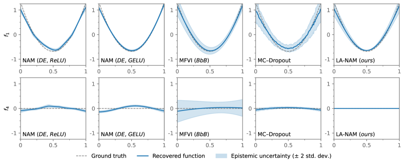
Figure B.1: Comparison of approximate inference methods for Bayesian NAMs on the synthetic data of Section 4.1. All feature networks use one layer of 64 GELU units with the exception of the leftmost model, “NAM (DE, ReLU)”, which uses 64-64-32 ReLU units.

We provide a brief overview of alternative approximate inference methods which can be employed to quantify uncertainty of feature networks in Bayesian NAMs. Figure B.1 displays the recovered functions and predictive intervals generated using these methods on the toy example of Section 4.1.

Deep ensembles (DE).

The nam of Agarwal et al. (2021) effectively operates as a deep ensemble (Lakshminarayanan et al., 2017) even though the authors do not explicitly present it as such. In our experiments, we found that ensembles of feature networks using ReLU and GELU activation tend to exhibit a collapse of diversity in function space, as can be seen in the two leftmost panels of Figure B.1. D’Angelo & Fortuin (2021) also highlight this as a potential limitation of deep ensembles. The utilization of ExU activation proposed by Agarwal et al. (2021) partially restores diversity, and we focus on this configuration when comparing to the la-nam.

Mean-field variational inference (MFVI).

Variational inference can also be used to obtain independent approximate feature network posteriors. In early experiments, we tested the Bayes-by-Backprop (BbB) procedure of Blundell et al. (2015) and found that the method required significant manual tuning since the feature networks tended to either severely underfit the functions or the uncertainty. MFVI also yields log-marginal likelihood estimates, however their use in gradient-optimization of neural network hyperparameters appears to be limited.

MC-Dropout.

Dropout (Gal & Ghahramani, 2016) can be a simple way of introducing uncertainty awareness in the nam but its Bayesian interpretation is not as straightforward as that of the Laplace approximation. It requires multiple forward passes for inference and does not provide an inherent mechanism for feature selection.

B.2 Ablation of the Anion Gap in MIMIC-III

The anion gap is a measure of the difference between the serum concentration of sodium and the serum concentrations of chloride and bicarbonate, i.e. $\mathrm{anion\ gap}=[\mathrm{Na}^{+}]-([\mathrm{Cl}^{-}]+[\mathrm{HCO_{3}^{-}]}).$

Both low bicarbonate levels and thus high anion gap are indicators of acute metabolic acidosis. This is a known risk factor for intensive care mortality with very poor prognosis (Kraut & Madias, 2010, 2012). Figure B.2 shows that the predicted mortality risk increases steadily as the anion gap grows but becomes uncertain above 20 mEq/L due to low sample size.

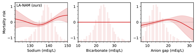
Figure B.2: Sodium, bicarbonate and anion gap mortality risk as predicted by the la-nam.

When presented with both anion gap and bicarbonate in the mortality risk dataset of Section 4.3, the la-nam uses high anion gap as a proxy for the risk of low bicarbonate. We confirm this visually by performing an ablation experiment in which the la-nam is re-trained with the feature network attending to the anion gap removed. Figure B.3 shows that in the ablated model the anion gap risk is moved into the low levels for bicarbonate. The bicarbonate risk increases below 20 mEq/L and becomes uncertain around 15 mEq/L.

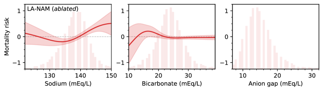
Figure B.3: Sodium and bicarbonate mortality risk with anion gap feature network ablated.

In contrast, the oak-gp does not suppress the bicarbonate, possibly indicating that the orthogonality constraint which it enforces has difficulty addressing redundancy of information when variables are highly correlated.

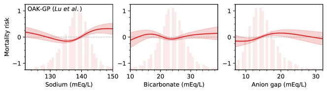
Figure B.4: Sodium, bicarbonate and anion gap mortality risk in the oak-gp of Lu et al. (2022).

B.3 Ablation of the Activation Function

In Figure B.5 and Table B.1, we progressively ablate the feature network depth and activation function of the nam to match ours. Shallow networks and GELU activation encourage smoother fits at the expense of worse predictive uncertainty and performance. This is not a concern for the la-nam when applied to the same architecture

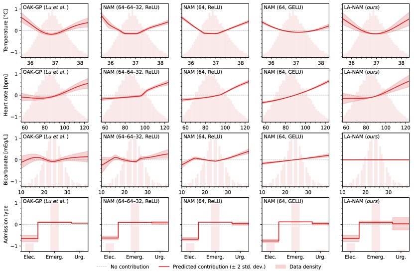
Figure B.5: Progressive ablation of the feature network depth and activation function on the MIMIC-III dataset of Section 4.3. Feature network architecture is denoted in parentheses. “la-nam (ours)” is a single layer of 64 GELU units.

Table B.1: Mean and standard errors over 5 runs for the performance of the ablated models shown in Figure B.5.

MIMIC-III Performance AUROC ($\uparrow$) AUPRC ($\uparrow$) NLL ($\downarrow$) nam (64–64–32, ReLU) 78.89 (±0.04) 34.30 (±0.04) 0.2669 (±2e-4) nam (64, ReLU) 79.02 (±0.02) 34.28 (±0.02) 0.2665 (±1e-4) nam (64, GELU) 77.54 (±0.02) 34.10 (±0.02) 0.2699 (±1e-4) la-nam (64, GELU) 79.58 (±0.01) 34.77 (±0.04) 0.2644 (±1e-4)

B.4 Calibration on the ICU Mortality Prediction Tasks

We assess the calibration of the nam and la-nam predictions on the ICU mortality tasks of Section 4.3. Following the protocol introduced by Ciosek et al. (2020), we present the accuracy as a function of subsets of retained test points in Figure B.6. The points are first sorted based on the confidence level of the models and then progressively added to the subset to determine a rolling accuracy. The median of the rolling accuracy curves for 5 independent runs is shown. On the MIMIC-III dataset, the la-nam demonstrates superior calibration compared to the nam, and it exhibits similar calibration on the significantly larger HiRID ICU dataset. Importantly, the incorporation of feature interactions does not seem to adversely harm calibration.

In Table B.2, we report mean calibration errors and their respective standard errors over the same 5 independent runs. We provide both the standard expected calibration error (ECE) of Guo et al. (2017), and the root Brier score (RBS), a proper calibration error put forward by Gruber & Buettner (2022). Bold values signify best calibration within one standard error, with the exception of la-nam₁₀ where bold indicates on par or better calibration compared to the first-order methods.

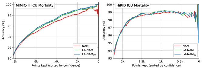
Figure B.6: Calibration curves of the mortality prediction models showing the relationship between uncertainty (horizontal axis) and accuracy (vertical axis). In well-calibrated models, accuracy should increase monotonically.

Table B.2: Calibration errors over the 5 runs of the mortality models assessed in Figure B.6.

Model nam la-nam la-nam₁₀ Metric ECE ($\downarrow$) RBS ($\downarrow$) ECE ($\downarrow$) RBS ($\downarrow$) ECE ($\downarrow$) RBS ($\downarrow$) MIMIC-III ICU Mortality 0.019 ±3.7e-4 0.279 ±1.2e-5 0.009 ±1.6e-4 0.275 ±2.5e-5 0.009 ±6.7e-4 0.275 ±9.6e-5 HiRID ICU Mortality 0.029 ±2.4e-3 0.223 ±3.7e-4 0.009 ±3.3e-4 0.219 ±1.6e-4 0.011 ±4.9e-4 0.219 ±2.3e-4

B.5 Calibration on UCI Datasets

We also provide calibration errors and respective standard errors for the 5-fold UCI benchmarks in Tables B.3 and B.4. For the UCI classification datasets we reuse the metrics of Section B.4, namely the expected calibration error (ECE) of Guo et al. (2017) and the root Brier score (RBS) proposed by Gruber & Buettner (2022). In UCI regression, we provide the quantile error metric proposed by Kuleshov et al. (2018) which we denote as “Calib.” We also present the squared kernel calibration error for Gaussian predictions (SKCE) proposed by Widmann et al. (2022). Similarly to Section B.4, bold denotes best within first-order methods with the exception of la-nam₁₀ where bold means on-par or better.

Table B.3: Calibration error on UCI regression datasets. (Lower is better.)

Model nam la-nam la-nam₁₀ Metric Calib. ($\downarrow$) SKCE ($\downarrow$) Calib. ($\downarrow$) SKCE ($\downarrow$) Calib. ($\downarrow$) SKCE ($\downarrow$) autompg ($n=392$) 0.054 ±0.011 1.9e-3 ±7.0e-4 0.037 ±0.007 1.8e-3 ±3.5e-4 0.043 ±0.009 1.5e-3 ±4.4e-4 concrete ($n=1030$) 0.021 ±0.007 6.2e-4 ±1.6e-4 0.014 ±0.004 6.2e-4 ±1.3e-4 0.015 ±0.005 6.5e-4 ±1.2e-4 energy ($n=768$) 0.042 ±0.018 8.3e-3 ±4.8e-4 0.040 ±0.010 8.9e-3 ±4.1e-4 0.042 ±0.014 6.1e-3 ±1.3e-3 kin8nm ($n=8192$) 0.015 ±0.002 5.6e-5 ±1.0e-5 0.012 ±0.001 2.7e-6 ±4.4e-6 0.007 ±0.001 1.4e-5 ±4.5e-6 naval ($n=11934$) 0.176 ±0.006 3.1e-8 ±4.4e-9 0.077 ±0.029 2.7e-9 ±1.5e-10 0.026 ±0.004 2.2e-9 ±1.8e-11 power ($n=9568$) 0.005 ±0.002 2.3e-4 ±3.1e-5 0.005 ±0.002 1.9e-4 ±1.3e-5 0.008 ±0.001 1.7e-4 ±1.5e-5 protein ($n=45730$) 0.037 ±0.003 1.8e-2 ±2.5e-4 0.020 ±0.002 1.5e-2 ±2.7e-4 0.015 ±0.000 1.5e-2 ±1.5e-4 wine ($n=1599$) 0.021 ±0.002 1.7e-3 ±5.6e-4 0.012 ±0.005 6.9e-4 ±3.2e-4 0.010 ±0.004 5.8e-4 ±3.1e-4 yacht ($n=308$) 0.095 ±0.027 1.8e-2 ±2.0e-3 0.105 ±0.028 1.7e-2 ±2.3e-3 0.111 ±0.024 1.2e-3 ±1.6e-4

Table B.4: Calibration error on UCI classification datasets. (Lower is better.)

Model nam la-nam la-nam₁₀ Metric ECE ($\downarrow$) RBS ($\downarrow$) ECE ($\downarrow$) RBS ($\downarrow$) ECE ($\downarrow$) RBS ($\downarrow$) australian ($n=690$) 0.112 ±0.008 0.330 ±0.017 0.099 ±0.004 0.314 ±0.014 0.084 ±0.004 0.317 ±0.015 breast ($n=569$) 0.064 ±0.018 0.192 ±0.013 0.038 ±0.005 0.163 ±0.010 0.040 ±0.004 0.165 ±0.009 heart ($n=270$) 0.153 ±0.008 0.356 ±0.020 0.136 ±0.011 0.314 ±0.014 0.150 ±0.015 0.315 ±0.015 ionosphere ($n=351$) 0.111 ±0.014 0.292 ±0.014 0.086 ±0.012 0.266 ±0.022 0.080 ±0.006 0.270 ±0.015 parkinsons ($n=195$) 0.139 ±0.006 0.290 ±0.019 0.136 ±0.009 0.280 ±0.023 0.111 ±0.006 0.277 ±0.025

B.6 Additional Results on UCI Datasets and ICU Mortality Tasks

In this section, we report the mean performance and standard errors for additional models and metrics over the 5-fold cross-validation UCI benchmarks of Section 4.2 and ICU mortality tasks of Section 4.3. Bolded values indicate best performance within additive models, and green or red an improvement or decrease beyond one standard error when second-order interactions are added. In addition to the models of Table 1, we give performance for linear and logistic regression, the smoothing-spline gam, and the la-nam with 10 interactions selected using the improvement to the marginal likelihood lower bound which is discussed in Section A.2.2 and denoted as la-nam${}_{\mathrm{10}}^{\dagger}$, instead of the MI-based selection presented in Section 3.2.3. We also benchmark against the gradient boosting-based explainable boosting model (ebm) (Lou et al., 2012; Nori et al., 2019), which is assigned a maximum likelihood fit of the observation noise in regression using its training data and also supports selection of top-10 feature interaction pairs (denoted as ebm₁₀).

Table B.5: Performance of the ebm on the mortality tasks of Section 4.3.

Task	MIMIC-III ICU Mortality			HiRID ICU Mortality
Metric	AUROC ($\uparrow$)	AUPRC ($\uparrow$)	NLL ($\downarrow$)	AUROC ($\uparrow$)	AUPRC ($\uparrow$)	NLL ($\downarrow$)
nam	77.6 ± 0.03	32.3 ± 0.03	0.274 ± 8e-5	89.6 ± 0.17	60.7 ± 0.14	0.228 ± 1e-2
la-nam	79.6 ± 0.01	34.8 ± 0.04	0.264 ± 5e-5	90.1 ± 0.03	60.5 ± 0.14	0.174 ± 2e-4
la-nam10	80.2 ± 0.10	35.2 ± 0.06	0.262 ± 3e-4	90.1 ± 0.01	60.5 ± 0.20	0.174 ± 4e-4
oak-gp	79.9 ± 0.03	35.2 ± 0.11	0.263 ± 1e-4	—	—	—
oak-gp*	71.7 ± 0.66	28.5 ± 0.42	0.288 ± 1e-3	—	—	—
ebm	78.7 ± 0.02	33.6 ± 0.04	0.268 ± 9e-5	90.2 ± 0.03	59.2 ± 0.10	0.177 ± 2e-4
ebm10	79.7 ± 0.03	34.9 ± 0.09	0.264 ± 2e-4	90.5 ± 0.04	61.1 ± 0.23	0.173 ± 4e-4
LightGBM	80.6 ± 0.08	35.6 ± 0.19	0.261 ± 3e-4	90.7 ± 0.00	61.6 ± 0.00	0.172 ± 0.00

B.7 Experimental Setup

Linear/Logistic Regression.

Implementations are provided by the scikit-learn library (Pedregosa et al., 2011). The regularization strength is grid-searched in the set $\{0.001,0.01,0.1,1,10\}$. For logistic regression, we use the L-BFGS solver performing up to 10,000 iterations.

GAM.

We use an open source Python implementation (pygam; Servén et al., 2018). The smoothing parameters are grid-searched: We sample one thousand candidates uniformly from the recommended range of $[10^{-3},\,10^{3}]$ and select using generalized cross-validation scoring (GCV; Golub et al., 1979).

NAM.

We test the NAM with feature networks containing a single hidden layer of 1024 units and ExU activation. We grid-search the learning rate and regularization hyperparameters using the values given in the supplementary material of Agarwal et al. (2021). In practice, we find that combining dropout with a probability of 0.2 and feature dropout of 0.05 along with weight decay of $10^{-5}$ and a learning rate of either 0.01 or 0.001 gave good results.

LA-NAM.

The la-nam is constructed using feature networks containing a single hidden layer of 64 neurons with GELU activation (Hendrycks & Gimpel, 2016). Joint feature networks added for second-order interaction fine-tuning contain two hidden layers of 64 neurons. The feature network parameters and hyperparameters (prior precision, observation noise) are optimized using Adam (Kingma & Ba, 2014), alternating between optimizing both at regular intervals, as in Immer et al. (2021a). We select the learning rate in the discrete set of $\{0.1,\,0.01,\,0.001\}$ which maximizes the ultimate $\log$-marginal likelihood. We use a batch size of 512 and perform early stopping on the $\log$-marginal likelihood restoring the best scoring parameters and hyperparameters at the end of training. We find that the algorithm is fairly robust to the choice of hyperparameter optimization schedule: For all experiments, we use $0.1$ for the hyperparameter learning rate and perform batches of 30 gradient steps on the $\log$-marginal likelihood every 100 epochs of regular training.

OAK-GP.

We use the setup recommended by the authors (See Appendix H. of Lu et al., 2022). Sparse GP regression is used for large UCI regression datasets ($n\geq 1000$). For the UCI classification and ICU mortality prediction tasks variational inference is used, with 200 inducing points for UCI and 800 inducing points for the mortality prediction.

EBM.

The explainable boosting machine (ebm) is an open-source Python implementation of the gradient-boosting GAM that is available as a part of the InterpretML library (Nori et al., 2019). The library defaults for the hyperparameters performed best. We did not find a significant improvement when tuning the learning rate, maximum number of leaves, or minimum number of samples per leaf.

LightGBM.

We use the open-source implementation (Ke et al., 2017). The maximum depth of each tree is selected in the set $\{3,\,7,\,12\}$, and maximum number of leaves in the set $\{8,\,16,\,31\}$. Additionally, the minimum number of samples per leaf is reduced to 2 on small datasets from the default of 20. Early stopping is enabled in all experiments, using a 12.5% split of the training data when the task has no predefined validation data. For the HiRID ICU Mortality task in Table 2, we obtain best performance when using the feature engineering recommended in Yèche et al. (2021).

Hardware.

The deep learning models are trained on a single NVIDIA RTX2080Ti with a Xeon E5-2630v4 core. Other models are trained on Xeon E5-2697v4 cores and Xeon Gold 6140 cores.

B.8 Illustrative Example

In Section 4.1, we present an illustrative example to motivate the capacity of the la-nam and baselines to recover purely additive structure from noisy data. We provide further details on the generation of the synthetic dataset used here. Consider the function $\hat{f}:\mathbb{R}^{4}\to\mathbb{R}$, where $\hat{f}(x_{1},\,x_{2},\,x_{3},\,x_{4})=\hat{f}_{1}(x_{1})+\hat{f}_{2}(x_{2})+\hat{f}_{3}(x_{3})+\hat{f}_{4}(x_{4})$, and

$$\hat{f}_{1}(x_{1})=8(x_{1}-\tfrac{1}{2})^{2},\quad \hat{f}_{2}(x_{2})=\tfrac{1}{10}\exp[-8x_{2}+4]$$ (B.1)

$$\hat{f}_{3}(x_{3})=5\exp[-2(2x_{3}-1)^{2}],\quad \hat{f}_{4}(x_{4})=0.$$ (B.2)

We generate $N=1000$ noisy observations $\{\mathbf{x}_{n},\,y_{n}\}_{n=1}^{N}$ by sampling inputs $\mathbf{x}_{n}$ uniformly from $\mathcal{U}([0,\,1]^{4})$ and generating targets $y_{n}=\hat{f}(\mathbf{x}_{n})+\epsilon_{n}$, where $\epsilon_{n}\sim\mathcal{N}(0,\,1)$ is random Gaussian noise. Figure B.7 shows the recovered functions along with the associated predictive uncertainty for the la-nam and baseline models.

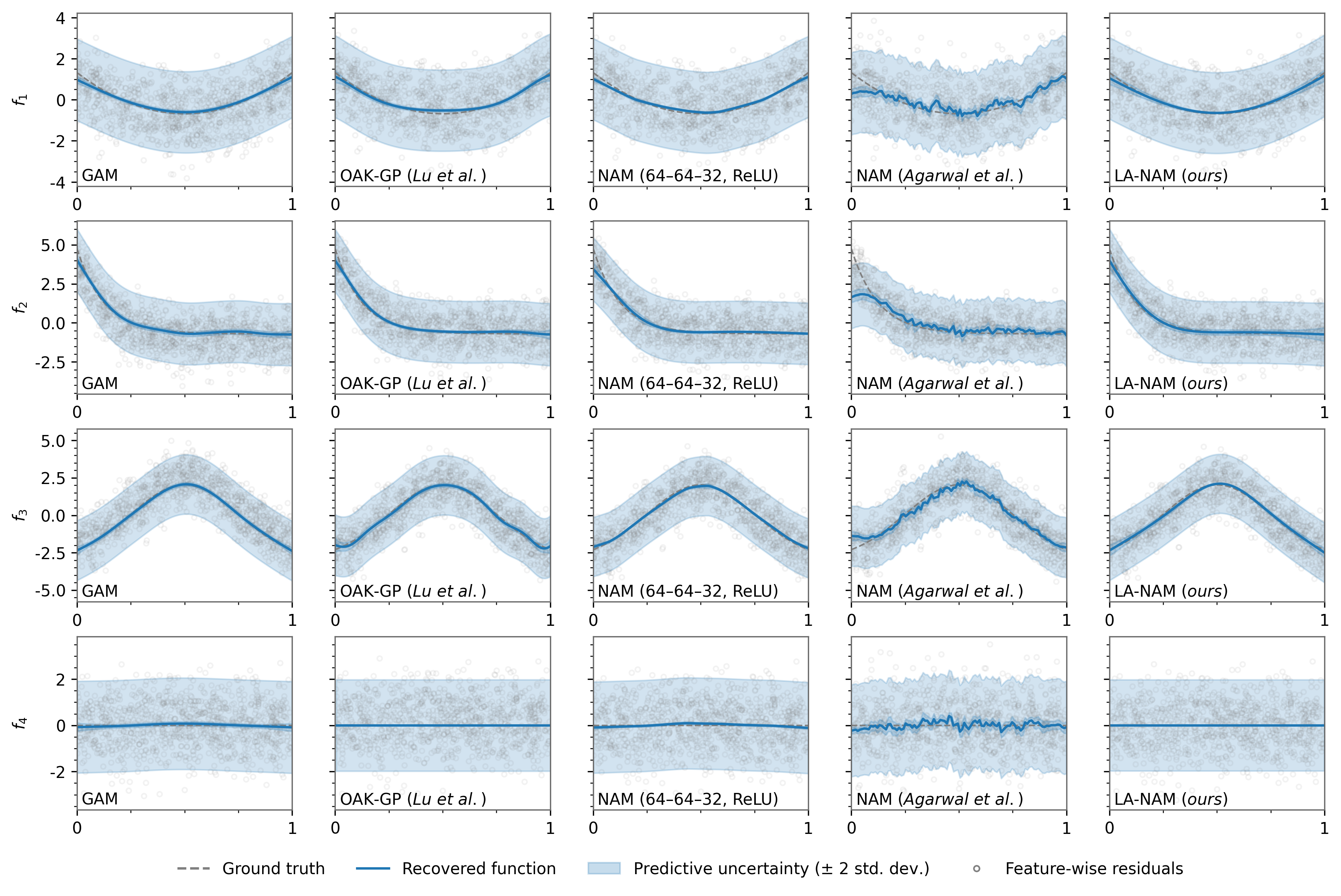
Figure B.7: Recovery of the additive structure of the synthetic dataset of B.8. The feature-wise residuals are the generated data points with mean contribution of the other feature networks subtracted.

B.9 Predicted Mortality Risk in MIMIC-III

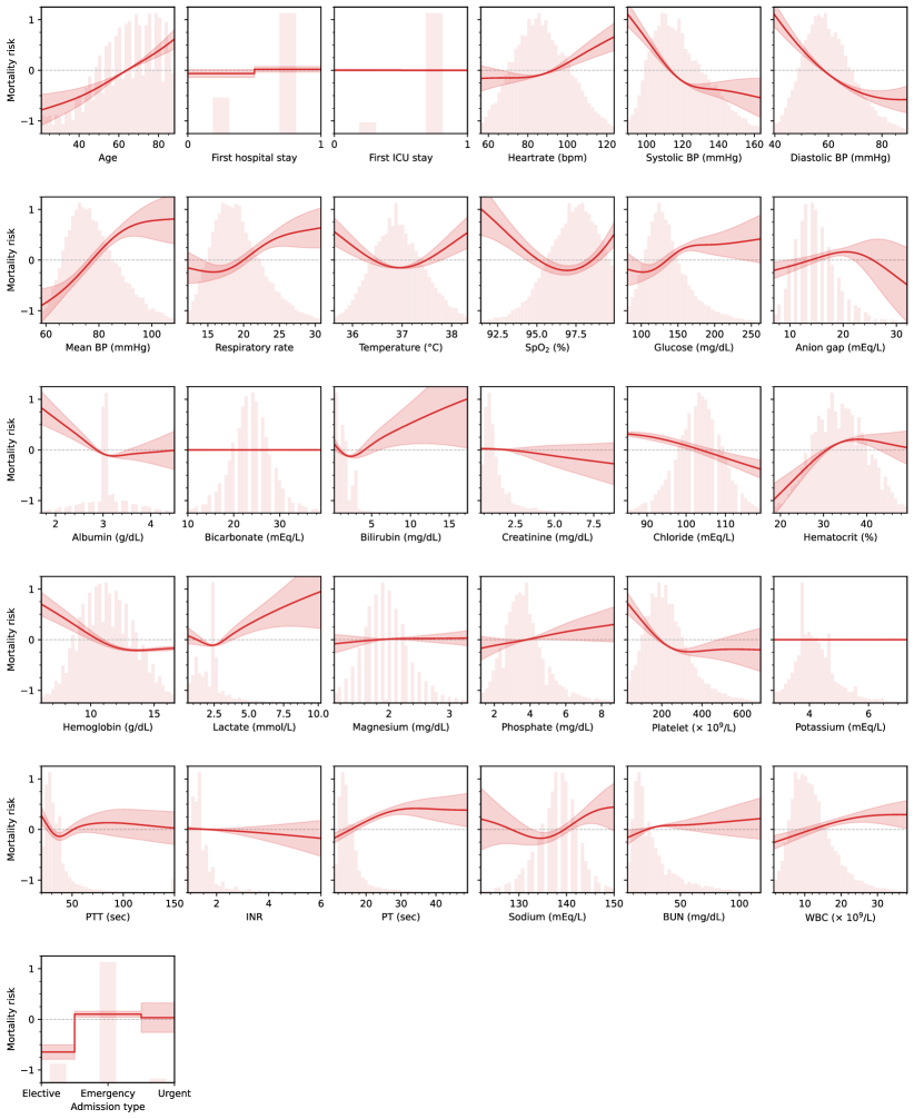
Figure B.8: Complete visualization of the la-nam predicted risk in the MIMIC-III mortality task of Section 4.3.

Appendix C Detailed Related Work

Generalized additive models.

Generalized additive models have been extensively studied and various approaches have been proposed for their construction. Hastie & Tibshirani (1999) initially suggested using smoothing splines (Wahba, 1983) to build the smoothing functions which attend to each feature, fitting them iteratively through “backfitting” (Breiman & Friedman, 1985). One alternative is to construct them using gradient-boosted decision trees (Friedman, 2001). By modifying the boosting algorithm, it becomes possible to cycle through functions in the inner loop, which has been found to be favorable compared to sequential backfitting of boosted trees (Lou et al., 2012). Furthermore, boosted trees facilitate the selection and fitting of feature interactions (Lou et al., 2013). These second-order interactions are believed to contribute to the competitive accuracy achieved by gradient-boosted additive models in comparison to fully interacting models for tabular supervised learning (Caruana et al., 2015; Nori et al., 2019).

Neural additive models.

Neural networks are highly attractive for constructing smoothing functions due to their ability to approximate continuous functions with arbitrary precision given sufficient complexity (Cybenko, 1989; Maiorov & Pinkus, 1999; Lu et al., 2017). Agarwal et al. (2021) proposed the neural additive model (NAM), which utilizes ensembles of feed-forward networks and employs standard backpropagation for fitting. To accommodate jagged functions, they introduced “ExU” dense layers, wherein weights are learned in logarithmic space.

A closely related model, called GAMI-Net, was introduced by Yang et al. (2021), but it employs single networks instead of an ensemble and additionally supports the learning of feature interaction terms. In the GAMI-Net, the feature pair candidates are selected for feature interaction fine-tuning using the ranking procedure of Lou et al. (2013). Yang et al. (2021) acknowledge that this ranking can also be done using neural networks with the approach proposed by Tsang et al. (2018). Alternatively, one can avoid having to select pairs entirely by finding a scalable formulation for all possible pairs, such as in the neural basis model (NBM) of Radenovic et al. (2022). In this work, we propose to rank the feature pair candidates using the available posterior approximation.

Many other extensions have been suggested, including feature selection through sparse regularization of the feature networks (Xu et al., 2022), generation of confidence intervals using regression spline basis expansion (Luber et al., 2023), and estimation of the skewness, heteroscedasticity, and kurtosis of the underlying data distributions (Thielmann et al., 2023).

Bayesian neural networks.

Bayesian neural networks offer the potential to combine the expressive capabilities of neural networks with the rigorous statistical properties of Bayesian inference (MacKay, 1992; Neal, 1993). However, achieving accurate inference in these complex models has proven to be a challenging endeavor (Jospin et al., 2022). The field has explored various techniques for approximate inference, each with its own trade-offs in terms of quality and computational cost.

At one end of the spectrum, we have inexpensive local approximations such as Laplace inference (Laplace, 1774; MacKay, 1992; Khan et al., 2019; Daxberger et al., 2021b) which provides a simple and computationally efficient solution. Other approaches in this category include stochastic weight averaging (Izmailov et al., 2018; Maddox et al., 2019) and dropout (Gal & Ghahramani, 2016; Kingma et al., 2015).

Moving towards more sophisticated approximations, variational methods come into play, offering a range of complexity levels. Researchers have proposed diverse variational approximations, including work by Graves (2011); Blundell et al. (2015); Louizos & Welling (2016); Khan et al. (2018); Osawa et al. (2019). Ensemble-based methods have also been explored as an alternative avenue. This includes recent work by Lakshminarayanan et al. (2017); Wang et al. (2019); Wilson & Izmailov (2020); Ciosek et al. (2020); He et al. (2020); D’Angelo et al. (2021); D’Angelo & Fortuin (2021).

On the other end of the spectrum, we find Markov Chain Monte Carlo (MCMC) approaches, which provide asymptotically correct solutions. Neal (1993); Neal et al. (2011); Welling & Teh (2011); Garriga-Alonso & Fortuin (2021); Izmailov et al. (2021) have contributed to the exploration of these computationally expensive yet theoretically accurate methods.

Beyond the challenges related to approximate inference, recent work has also studied the question of prior choice for Bayesian neural networks (e.g., Fortuin et al., 2021, 2022; Fortuin, 2022; Nabarro et al., 2022; Sharma et al., 2023, and references therein). Additionally, model selection within the Bayesian neural network framework has garnered attention (e.g., Immer et al., 2021a, 2022b, 2022a; Rothfuss et al., 2021, 2022; van der Ouderaa & van der Wilk, 2022; Schwöbel et al., 2022).

In our work, we focus primarily on leveraging the linearized Laplace inference technique proposed by Immer et al. (2021b). We also utilize the associated marginal likelihood estimation method introduced by Immer et al. (2021a). These methods, to the best of our knowledge, have not been previously applied to the NAM.

References

- Agarwal et al. (2021) Agarwal, R., Melnick, L., Frosst, N., Zhang, X., Lengerich, B., Caruana, R., and Hinton, G. E. Neural Additive Models: Interpretable Machine Learning with Neural Nets. In Advances in Neural Information Processing Systems, volume 34, pp. 4699–4711. Curran Associates, Inc., 2021.
- Antorán et al. (2022) Antorán, J., Janz, D., Allingham, J. U., Daxberger, E., Barbano, R. R., Nalisnick, E., and Hernández-Lobato, J. M. Adapting the linearised laplace model evidence for modern deep learning. In International Conference on Machine Learning, pp. 796–821. PMLR, 2022.
- Baughman et al. (1993) Baughman, R. R., Lower, E. E., Flessa, H. C., and Tollerud, D. J. Thrombocytopenia in the intensive care unit. Chest, 104(4):1243–1247, 1993.
- Blundell et al. (2015) Blundell, C., Cornebise, J., Kavukcuoglu, K., and Wierstra, D. Weight uncertainty in neural networks. In ICML, 2015.
- Breiman & Friedman (1985) Breiman, L. and Friedman, J. H. Estimating Optimal Transformations for Multiple Regression and Correlation. Journal of the American Statistical Association, 80(391):580–598, September 1985. ISSN 0162-1459. doi: 10.1080/01621459.1985.10478157.
- Caruana et al. (2015) Caruana, R., Lou, Y., Gehrke, J., Koch, P., Sturm, M., and Elhadad, N. Intelligible Models for HealthCare: Predicting Pneumonia Risk and Hospital 30-day Readmission. In Proceedings of the 21th ACM SIGKDD International Conference on Knowledge Discovery and Data Mining, KDD ’15, pp. 1721–1730, New York, NY, USA, August 2015. Association for Computing Machinery. ISBN 978-1-4503-3664-2. doi: 10.1145/2783258.2788613.
- Ciosek et al. (2020) Ciosek, K., Fortuin, V., Tomioka, R., Hofmann, K., and Turner, R. Conservative uncertainty estimation by fitting prior networks. In International Conference on Learning Representations, 2020.
- Cooper & Ghanima (2019) Cooper, N. and Ghanima, W. Immune thrombocytopenia. New England Journal of Medicine, 381(10):945–955, 2019.
- Cybenko (1989) Cybenko, G. Approximation by superpositions of a sigmoidal function. Mathematics of Control, Signals and Systems, 2(4):303–314, December 1989. ISSN 1435-568X. doi: 10.1007/BF02551274.
- D’Angelo & Fortuin (2021) D’Angelo, F. and Fortuin, V. Repulsive deep ensembles are bayesian. Advances in Neural Information Processing Systems, 34:3451–3465, 2021.
- D’Angelo et al. (2021) D’Angelo, F., Fortuin, V., and Wenzel, F. On stein variational neural network ensembles. arXiv preprint arXiv:2106.10760, 2021.
- Daxberger et al. (2021a) Daxberger, E., Kristiadi, A., Immer, A., Eschenhagen, R., Bauer, M., and Hennig, P. Laplace redux-effortless bayesian deep learning. Advances in Neural Information Processing Systems, 34:20089–20103, 2021a.
- Daxberger et al. (2021b) Daxberger, E., Kristiadi, A., Immer, A., Eschenhagen, R., Bauer, M., and Hennig, P. Laplace Redux - Effortless Bayesian Deep Learning. In Advances in Neural Information Processing Systems, volume 34, pp. 20089–20103. Curran Associates, Inc., 2021b.
- Daxberger et al. (2021c) Daxberger, E., Nalisnick, E., Allingham, J. U., Antorán, J., and Hernández-Lobato, J. M. Bayesian deep learning via subnetwork inference. In International Conference on Machine Learning, pp. 2510–2521. PMLR, 2021c.
- Durrande et al. (2012) Durrande, N., Ginsbourger, D., and Roustant, O. Additive Covariance kernels for high-dimensional Gaussian Process modeling. Annales de la Faculté des sciences de Toulouse : Mathématiques, 21(3):481–499, 2012. ISSN 2258-7519. doi: 10.5802/afst.1342.
- Duvenaud et al. (2011) Duvenaud, D. K., Nickisch, H., and Rasmussen, C. Additive gaussian processes. In Shawe-Taylor, J., Zemel, R., Bartlett, P., Pereira, F., and Weinberger, K. (eds.), Advances in Neural Information Processing Systems, volume 24. Curran Associates, Inc., 2011.
- Faltys et al. (2021) Faltys, M., Zimmermann, M., Lyu, X., Hüser, M., Hyland, S., Rätsch, G., and Merz, T. Hirid, a high time-resolution icu dataset (version 1.1.1). PhysioNet, 2021.
- Foong et al. (2019) Foong, A. Y., Li, Y., Hernández-Lobato, J. M., and Turner, R. E. ’in-between’uncertainty in bayesian neural networks. arXiv preprint arXiv:1906.11537, 2019.
- Fortuin (2022) Fortuin, V. Priors in bayesian deep learning: A review. International Statistical Review, 90(3):563–591, 2022.
- Fortuin et al. (2021) Fortuin, V., Garriga-Alonso, A., van der Wilk, M., and Aitchison, L. Bnnpriors: A library for bayesian neural network inference with different prior distributions. Software Impacts, 9:100079, 2021.
- Fortuin et al. (2022) Fortuin, V., Garriga-Alonso, A., Ober, S. W., Wenzel, F., Ratsch, G., Turner, R. E., van der Wilk, M., and Aitchison, L. Bayesian neural network priors revisited. In International Conference on Learning Representations, 2022.
- Friedman (2001) Friedman, J. H. Greedy Function Approximation: A Gradient Boosting Machine. The Annals of Statistics, 29(5):1189–1232, 2001. ISSN 0090-5364.
- Gal & Ghahramani (2016) Gal, Y. and Ghahramani, Z. Dropout as a Bayesian approximation: Representing model uncertainty in deep learning. In ICML, 2016.
- Garriga-Alonso & Fortuin (2021) Garriga-Alonso, A. and Fortuin, V. Exact Langevin dynamics with stochastic gradients. arXiv preprint arXiv:2102.01691, 2021.
- Golub et al. (1979) Golub, G. H., Heath, M., and Wahba, G. Generalized Cross-Validation as a Method for Choosing a Good Ridge Parameter. Technometrics, 21(2):215–223, May 1979. ISSN 0040-1706, 1537-2723. doi: 10.1080/00401706.1979.10489751.
- Graves (2011) Graves, A. Practical variational inference for neural networks. In NIPS, 2011.
- Grinsztajn et al. (2022) Grinsztajn, L., Oyallon, E., and Varoquaux, G. Why do tree-based models still outperform deep learning on tabular data? arXiv preprint arXiv:2207.08815, 2022.
- Gruber & Buettner (2022) Gruber, S. and Buettner, F. Better uncertainty calibration via proper scores for classification and beyond. Advances in Neural Information Processing Systems, 35:8618–8632, 2022.
- Guo et al. (2017) Guo, C., Pleiss, G., Sun, Y., and Weinberger, K. Q. On calibration of modern neural networks. In International conference on machine learning, pp. 1321–1330. PMLR, 2017.
- Hastie & Tibshirani (1999) Hastie, T. and Tibshirani, R. Generalized Additive Models. Chapman & Hall/CRC, Boca Raton, Fla, 1999. ISBN 978-0-412-34390-2.
- He et al. (2020) He, B., Lakshminarayanan, B., and Teh, Y. W. Bayesian deep ensembles via the neural tangent kernel. Advances in neural information processing systems, 33:1010–1022, 2020.
- Hendrycks & Gimpel (2016) Hendrycks, D. and Gimpel, K. Gaussian error linear units (gelus). arXiv preprint arXiv:1606.08415, 2016.
- Immer et al. (2021a) Immer, A., Bauer, M., Fortuin, V., Rätsch, G., and Khan, M. E. Scalable marginal likelihood estimation for model selection in deep learning. In ICML, 2021a.
- Immer et al. (2021b) Immer, A., Korzepa, M., and Bauer, M. Improving predictions of Bayesian neural nets via local linearization. In Proceedings of The 24th International Conference on Artificial Intelligence and Statistics, pp. 703–711. PMLR, March 2021b.
- Immer et al. (2022a) Immer, A., Hennigen, L. T., Fortuin, V., and Cotterell, R. Probing as quantifying inductive bias. In Proceedings of the 60th Annual Meeting of the Association for Computational Linguistics (Volume 1: Long Papers), pp. 1839–1851, 2022a.
- Immer et al. (2022b) Immer, A., van der Ouderaa, T. F., Fortuin, V., Rätsch, G., and van der Wilk, M. Invariance learning in deep neural networks with differentiable Laplace approximations. In NeurIPS, 2022b.
- Immer et al. (2023) Immer, A., Van Der Ouderaa, T. F., Van Der Wilk, M., Ratsch, G., and Schölkopf, B. Stochastic marginal likelihood gradients using neural tangent kernels. In International Conference on Machine Learning, pp. 14333–14352. PMLR, 2023.
- Izmailov et al. (2018) Izmailov, P., Podoprikhin, D., Garipov, T., Vetrov, D., and Wilson, A. G. Averaging weights leads to wider optima and better generalization. In 34th Conference on Uncertainty in Artificial Intelligence 2018, UAI 2018, pp. 876–885, 2018.
- Izmailov et al. (2021) Izmailov, P., Vikram, S., Hoffman, M. D., and Wilson, A. G. What are Bayesian neural network posteriors really like? In ICML, 2021.
- Johnson et al. (2016) Johnson, A. E. W., Pollard, T. J., Shen, L., Lehman, L.-w. H., Feng, M., Ghassem i, M., Moody, B., Szolovits, P., Anthony Celi, L., and Mark, R. G. MIMIC-III, a freely accessible critical care database. Scientific Data, 3(1):160035, May 2016. ISSN 2052-4463. doi: 10.1038/sdata.2016.35.
- Jospin et al. (2022) Jospin, L. V., Laga, H., Boussaid, F., Buntine, W., and Bennamoun, M. Hands-on bayesian neural networks - a tutorial for deep learning users. IEEE Computational Intelligence Magazine, 17(2):29–48, 2022.
- Kaufman & Sain (2010) Kaufman, C. G. and Sain, S. R. Bayesian functional {ANOVA} modeling using Gaussian process prior distributions. Bayesian Analysis, 5(1):123–149, March 2010. ISSN 1936-0975, 1931-6690. doi: 10.1214/10-BA505.
- Ke et al. (2017) Ke, G., Meng, Q., Finley, T., Wang, T., Chen, W., Ma, W., Ye, Q., and Liu, T.-Y. LightGBM: A Highly Efficient Gradient Boosting Decision Tree. In Advances in Neural Information Processing Systems, volume 30. Curran Associates, Inc., 2017.
- Khan et al. (2018) Khan, M., Nielsen, D., Tangkaratt, V., Lin, W., Gal, Y., and Srivastava, A. Fast and scalable Bayesian deep learning by weight-perturbation in Adam. In ICML, 2018.
- Khan et al. (2019) Khan, M. E., Immer, A., Abedi, E., and Korzepa, M. Approximate inference turns deep networks into Gaussian processes. In NeurIPS, 2019.
- Kingma & Ba (2014) Kingma, D. P. and Ba, J. Adam: A method for stochastic optimization. arXiv preprint arXiv:1412.6980, 2014.
- Kingma et al. (2015) Kingma, D. P., Salimans, T., and Welling, M. Variational dropout and the local reparameterization trick. In Advances in Neural Information Processing Systems 28, 2015.
- Kraut & Madias (2010) Kraut, J. A. and Madias, N. E. Metabolic acidosis: Pathophysiology, diagnosis and management. Nature Reviews Nephrology, 6(5):274–285, May 2010. ISSN 1759-507X. doi: 10.1038/nrneph.2010.33.
- Kraut & Madias (2012) Kraut, J. A. and Madias, N. E. Treatment of acute metabolic acidosis: A pathophysiologic approach. Nature Reviews. Nephrology, 8(10):589–601, October 2012. ISSN 1759-507X. doi: 10.1038/nrneph.2012.186.
- Kuleshov et al. (2018) Kuleshov, V., Fenner, N., and Ermon, S. Accurate uncertainties for deep learning using calibrated regression. In International conference on machine learning, pp. 2796–2804. PMLR, 2018.
- Lakshminarayanan et al. (2017) Lakshminarayanan, B., Pritzel, A., and Blundell, C. Simple and scalable predictive uncertainty estimation using deep ensembles. In NIPS, 2017.
- Laplace (1774) Laplace, P. S. Mémoire sur la probabilité des causes par les évènements. In Mémoires de l’Académie Royale Des Sciences de Paris (Savants Étrangers), volume 6, pp. 621–656. 1774.
- Lengerich et al. (2022) Lengerich, B. J., Caruana, R., Nunnally, M. E., and Kellis, M. Death by Round Numbers: Glass-Box Machine Learning Uncovers Biases in Medical Practice, November 2022.
- Lou et al. (2012) Lou, Y., Caruana, R., and Gehrke, J. Intelligible models for classification and regression. In Proceedings of the 18th ACM SIGKDD International Conference on Knowledge Discovery and Data Mining, KDD ’12, pp. 150–158, New York, NY, USA, August 2012. Association for Computing Machinery. ISBN 978-1-4503-1462-6. doi: 10.1145/2339530.2339556.
- Lou et al. (2013) Lou, Y., Caruana, R., Gehrke, J., and Hooker, G. Accurate intelligible models with pairwise interactions. In Proceedings of the 19th ACM SIGKDD International Conference on Knowledge Discovery and Data Mining, KDD ’13, pp. 623–631, New York, NY, USA, August 2013. Association for Computing Machinery. ISBN 978-1-4503-2174-7. doi: 10.1145/2487575.2487579.
- Louizos & Welling (2016) Louizos, C. and Welling, M. Structured and efficient variational deep learning with matrix Gaussian posteriors. In ICML, 2016.
- Lu et al. (2022) Lu, X., Boukouvalas, A., and Hensman, J. Additive Gaussian processes revisited. In Chaudhuri, K., Jegelka, S., Song, L., Szepesvari, C., Niu, G., and Sabato, S. (eds.), Proceedings of the 39th International Conference on Machine Learning, volume 162 of Proceedings of Machine Learning Research, pp. 14358–14383. PMLR, 17–23 Jul 2022.
- Lu et al. (2017) Lu, Z., Pu, H., Wang, F., Hu, Z., and Wang, L. The Expressive Power of Neural Networks: A View from the Width. In Advances in Neural Information Processing Systems, volume 30. Curran Associates, Inc., 2017.
- Luber et al. (2023) Luber, M., Thielmann, A., and Säfken, B. Structural Neural Additive Models: Enhanced Interpretable Machine Learning, February 2023.
- Lundberg & Lee (2017) Lundberg, S. M. and Lee, S.-I. A Unified Approach to Interpreting Model Predictions. In Advances in Neural Information Processing Systems, volume 30. Curran Associates, Inc., 2017.
- MacKay (1991) MacKay, D. J. C. Bayesian model comparison and backprop nets. In Moody, J., Hanson, S., and Lippmann, R. (eds.), Advances in Neural Information Processing Systems, volume 4. Morgan-Kaufmann, 1991.
- MacKay (1992) MacKay, D. J. C. A practical Bayesian framework for backpropagation networks. Neural Computation, 4(3), 1992.
- MacKay (1994) MacKay, D. J. C. Bayesian nonlinear modeling for the prediction competition. ASHRAE transactions, 100(2):1053–1062, 1994.
- Maddox et al. (2019) Maddox, W. J., Izmailov, P., Garipov, T., Vetrov, D. P., and Wilson, A. G. A simple baseline for Bayesian uncertainty in deep learning. In NeurIPS, 2019.
- Maiorov & Pinkus (1999) Maiorov, V. and Pinkus, A. Lower bounds for approximation by MLP neural networks. Neurocomputing, 25(1):81–91, April 1999. ISSN 0925-2312. doi: 10.1016/S0925-2312(98)00111-8.
- Martens & Grosse (2015) Martens, J. and Grosse, R. Optimizing Neural Networks with Kronecker-factored Approximate Curvature. In International conference on machine learning, pp. 2408–2417. PMLR, 2015.
- Nabarro et al. (2022) Nabarro, S., Ganev, S., Garriga-Alonso, A., Fortuin, V., van der Wilk, M., and Aitchison, L. Data augmentation in bayesian neural networks and the cold posterior effect. In Uncertainty in Artificial Intelligence, pp. 1434–1444. PMLR, 2022.
- Neal (1993) Neal, R. M. Bayesian learning via stochastic dynamics. In Advances in neural information processing systems, pp. 475–482, 1993.
- Neal (1995) Neal, R. M. Bayesian Learning for Neural Networks. PhD thesis, University of Toronto, 1995.
- Neal et al. (2011) Neal, R. M. et al. MCMC using Hamiltonian dynamics. Handbook of Markov Chain Monte Carlo, 2(11), 2011.
- Nori et al. (2019) Nori, H., Jenkins, S., Koch, P., and Caruana, R. InterpretML: A Unified Framework for Machine Learning Interpretability, September 2019.
- Osawa et al. (2019) Osawa, K., Swaroop, S., Khan, M. E. E., Jain, A., Eschenhagen, R., Turner, R. E., and Yokota, R. Practical deep learning with Bayesian principles. In NeurIPS, 2019.
- Pedregosa et al. (2011) Pedregosa, F., Varoquaux, G., Gramfort, A., Michel, V., Thirion, B., Grisel, O., Blondel, M., Prettenhofer, P., Weiss, R., Dubourg, V., Vanderplas, J., Passos, A., Cournapeau, D., Brucher, M., Perrot, M., and Duchesnay, E. Scikit-learn: Machine learning in Python. Journal of Machine Learning Research, 12:2825–2830, 2011.
- Pumplun et al. (2021) Pumplun, L., Fecho, M., Wahl, N., Peters, F., and Buxmann, P. Adoption of Machine Learning Systems for Medical Diagnostics in Clinics: Qualitative Interview Study. Journal of Medical Internet Research, 23(10):e29301, October 2021. doi: 10.2196/29301.
- Radenovic et al. (2022) Radenovic, F., Dubey, A., and Mahajan, D. Neural Basis Models for Interpretability. Advances in Neural Information Processing Systems, 35:8414–8426, December 2022.
- Ribeiro et al. (2016) Ribeiro, M. T., Singh, S., and Guestrin, C. “Why Should I Trust You?”: Explaining the Predictions of Any Classifier. In Proceedings of the 22nd ACM SIGKDD International Conference on Knowledge Discovery and Data Mining, KDD ’16, pp. 1135–1144, New York, NY, USA, August 2016. Association for Computing Machinery. ISBN 978-1-4503-4232-2. doi: 10.1145/2939672.2939778.
- Ritter et al. (2018) Ritter, H., Botev, A., and Barber, D. A Scalable Laplace Approximation for Neural Networks. In 6th International Conference on Learning Representations, ICLR 2018-Conference Track Proceedings, volume 6. International Conference on Representation Learning, 2018.
- Rothfuss et al. (2021) Rothfuss, J., Fortuin, V., Josifoski, M., and Krause, A. Pacoh: Bayes-optimal meta-learning with pac-guarantees. In International Conference on Machine Learning, pp. 9116–9126. PMLR, 2021.
- Rothfuss et al. (2022) Rothfuss, J., Josifoski, M., Fortuin, V., and Krause, A. Pac-bayesian meta-learning: From theory to practice. arXiv preprint arXiv:2211.07206, 2022.
- Rudin (2019) Rudin, C. Stop explaining black box machine learning models for high stakes decisions and use interpretable models instead. Nature Machine Intelligence, 1(5):206–215, 2019.
- Schwöbel et al. (2022) Schwöbel, P., Jørgensen, M., Ober, S. W., and Van Der Wilk, M. Last layer marginal likelihood for invariance learning. In International Conference on Artificial Intelligence and Statistics, pp. 3542–3555. PMLR, 2022.
- Servén et al. (2018) Servén, D., Brummitt, C., Abedi, H., and hlink. pyGAM: Generalized Additive Models in Python. Zenodo, October 2018.
- Sharma et al. (2023) Sharma, M., Rainforth, T., Teh, Y. W., and Fortuin, V. Incorporating unlabelled data into bayesian neural networks. arXiv preprint arXiv:2304.01762, 2023.
- Thielmann et al. (2023) Thielmann, A., Kruse, R.-M., Kneib, T., and Säfken, B. Neural Additive Models for Location Scale and Shape: A Framework for Interpretable Neural Regression Beyond the Mean, January 2023.
- Timonen et al. (2021) Timonen, J., Mannerström, H., Vehtari, A., and Lähdesmäki, H. Lgpr: An interpretable non-parametric method for inferring covariate effects from longitudinal data. Bioinformatics, 37(13):1860–1867, July 2021. ISSN 1367-4803. doi: 10.1093/bioinformatics/btab021.
- Tipping (2001) Tipping, M. E. Sparse bayesian learning and the relevance vector machine. Journal of machine learning research, 1(Jun):211–244, 2001.
- Trehel-Tursis et al. (2012) Trehel-Tursis, V., Louvain-Quintard, V., Zarrouki, Y., Imbert, A., Doubine, S., and Stéphan, F. Clinical and biologic features of patients suspected or confirmed to have heparin-induced thrombocytopenia in a cardiothoracic surgical icu. Chest, 142(4):837–844, 2012.
- Tsang et al. (2018) Tsang, M., Cheng, D., and Liu, Y. Detecting Statistical Interactions from Neural Network Weights, February 2018.
- van der Ouderaa & van der Wilk (2022) van der Ouderaa, T. F. and van der Wilk, M. Learning invariant weights in neural networks. In Uncertainty in Artificial Intelligence, pp. 1992–2001. PMLR, 2022.
- Veale et al. (2018) Veale, M., Van Kleek, M., and Binns, R. Fairness and Accountability Design Needs for Algorithmic Support in High-Stakes Public Sector Decision-Making. In Proceedings of the 2018 CHI Conference on Human Factors in Computing Systems, CHI ’18, pp. 1–14, New York, NY, USA, April 2018. Association for Computing Machinery. doi: 10.1145/3173574.3174014.
- Wahba (1983) Wahba, G. Bayesian “Confidence Intervals” for the Cross-Validated Smoothing Spline. Journal of the Royal Statistical Society: Series B (Methodological), 45(1):133–150, 1983. ISSN 2517-6161. doi: 10.1111/j.2517-6161.1983.tb01239.x.
- Wang et al. (2019) Wang, Z., Ren, T., Zhu, J., and Zhang, B. Function space particle optimization for bayesian neural networks. In International Conference on Learning Representations, 2019.
- Welling & Teh (2011) Welling, M. and Teh, Y. W. Bayesian learning via stochastic gradient langevin dynamics. In ICML, 2011.
- Widmann et al. (2022) Widmann, D., Lindsten, F., and Zachariah, D. Calibration tests beyond classification. arXiv preprint arXiv:2210.13355, 2022.
- Wilson & Izmailov (2020) Wilson, A. G. and Izmailov, P. Bayesian deep learning and a probabilistic perspective of generalization. In NeurIPS, 2020.
- Xu et al. (2022) Xu, S., Bu, Z., Chaudhari, P., and Barnett, I. J. Sparse Neural Additive Model: Interpretable Deep Learning with Feature Selection via Group Sparsity, February 2022.
- Yang et al. (2021) Yang, Z., Zhang, A., and Sudjianto, A. GAMI-Net: An Explainable Neural Network based on Generalized Additive Models with Structured Interactions. Pattern Recognition, 120:108192, December 2021. ISSN 0031-3203. doi: 10.1016/j.patcog.2021.108192.
- Yèche et al. (2021) Yèche, H., Kuznetsova, R., Zimmermann, M., Hüser, M., Lyu, X., Faltys, M., and Rätsch, G. HiRID-ICU-Benchmark — A Comprehensive Machine Learning Benchmark on High-resolution ICU Data. Proceedings of the Neural Information Processing Systems Track on Datasets and Benchmarks, 1, December 2021.