Generalizing Adam To Manifolds For Efficiently Training Transformers

Abstract

One of the primary reasons behind the success of neural networks has been the emergence of an array of new, highly-successful optimizers, perhaps most importantly the Adam optimizer. It is widely used for training neural networks, yet notoriously hard to interpret. Lacking a clear physical intuition, Adam is difficult to generalize to manifolds. Some attempts have been made to directly apply parts of the Adam algorithm to manifolds or to find an underlying structure, but a full generalization has remained elusive.

In this work a new approach is presented that leverages the special structure of the manifolds which are relevant for optimization of neural networks, such as the Stiefel manifold, the symplectic Stiefel manifold, the Grassmann manifold and the symplectic Grassmann manifold: all of these are homogeneous spaces and as such admit a global tangent space representation.

This global tangent space representation is used to perform all of the steps in the Adam optimizer. The resulting algorithm is then applied to train a transformer for which orthogonality constraints are enforced up to machine precision and we observe significant speed-ups in the training process.

Keywords: Adam optimizer, neural network training, manifold optimization, Stiefel manifold, homogeneous spaces, deep learning, deep neural networks, transformer, orthogonality constraints, vanishing gradients, parallel programming

MSC 2020: 53Z50, 53C30, 68T07, 68W10, 90C26

1 Introduction and Related Work

The enormous success of neural networks in recent years has in large part been driven by the development of new and successful optimizers, most importantly Adam [22]. Even though the Adam algorithm is nowadays used to train a wide variety of neural networks, its theoretical properties remain largely obscure [24].

Besides new optimizers, another source of advancement in neural network research has been the inclusion of specific problem-dependent penalization terms into the loss functional. Two of the most important ones are (i) orthogonality constraints (see [32] for an application to transformer neural networks) and (ii) properties relating to a physical system, yielding physics-informed neural networks (PINNs, [29]). Despite successful application in many different settings, an inherent problem is that these regularizers do not provide theoretical guarantees on the preservation of the relevant properties and that they rely on extensive hyperparameter tuning. This makes training neural networks difficult, cumbersome and unpredictable.

What would make these extra terms in the loss functional and the associated hyperparameters redundant would be optimization on spaces that satisfy the associated constraints automatically [3, 25, 23, 26]. Such spaces are in many cases homogeneous spaces (see [28, Chapter 11] and [17, Chapter 17]), a special class of manifolds. Homogeneous spaces that are important for neural networks are the Stiefel manifold, the symplectic Stiefel manifold and the symplectic Grassmann manifold [4, 18]. Regarding point (i), it will be shown in section 4 that optimization on spaces that preserve orthonormality can enable training, or speed it up in other cases (see [23]). For point (ii), the case when the network has to be imbued with physical properties, optimizing on manifolds can be inevitable. This is crucial for “symplectic autoencoders” (see [10]) and also used for “structure-preserving transformers” (see [11]).

In order to fully benefit from introducing manifolds into neural networks, existing powerful optimizers should be extended to this setting, but the obscure nature of the Adam algorithm has meant that its properties have to be severely restricted before this extension can be made.

A first, partly successful, attempt at generalizing Adam is shown in [25], but does not capture the structure of the second moments (see eq. 7). The approach presented in [23] is more involved and the most-closely related one to this work. The authors formulate the optimization problem as an unconstrained variational problem with the corresponding Lagrangian on the Stiefel manifold $\mathcal{M}:=\{Y\in\mathbb{R}^{N\times{}n}:Y^{T}Y=\mathbb{I}_{n}\}$:

$$\mathfrak{L}(Y,\dot{Y},\Lambda,t)=r(t)\left[\frac{1}{2}\mathrm{Tr}\left(\dot{Y}^{T}(\mathbb{I}_{N}-aYY^{T})\dot{Y}\right)-L(Y)\right]-\frac{1}{2}\mathrm{Tr}\left(\bar{A}^{T}(Y^{T}Y-\mathbb{I}_{n})\right),$$ (1)

where $a$ is a parameter that defines a “one-parameter family of Riemannian metrics” on the Stiefel manifold $\mathcal{M}$, i.e. $g_{a}:T_{Y}\mathcal{M}\times{}T_{Y}\mathcal{M}\to\mathbb{R}^{+},\,(V_{1},V_{2})\mapsto\frac{1}{2}\mathrm{Tr}(V_{1}^{T}(\mathbb{I}_{n}-aYY^{T})V_{2})$, and $L$ is the loss function to be minimized. In this description $Y$, which are elements of $\mathcal{M}$, are parameters of the neural network and $\bar{A}\in\mathbb{R}^{n\times{}n}$ is a Lagrange multiplier that enforces the constraint such that the neural network weights are elements of a manifold.

The authors obtain equations of motion through the variational principle and these are then discretized by a clever splitting scheme to obtain the final optimizer, which is used for training the neural network. Stochastic gradient descent (SGD) with momentum is in this case just the solution of the variational problem, which the authors call “Momentum SGD”. In order to obtain a version of Adam, the authors apply a modification to this algorithm to include second moments. This step, however, involves a projection and thus does not generalize Adam completely. As for applications, the authors’ main practical objective is, as it is in this paper, to train a transformer [31].

The remainder of this paper is organized as follows: section 2 presents a high-level description of our approach and discusses the associated operations in some detail. It is shown how Adam can be recovered as a special case of this. Section 3 gives a description of all the relevant aspects of homogeneous spaces that are needed for our framework and section 4 shows an application of the new optimizers for training a transformer. The new optimizers are part of the Julia package GeometricMachineLearning.jl.

Throughout the discussion, the Stiefel manifold will be used as an example to elucidate the more abstract and general concepts; however the mathematical constructions are very general and can, in addition to the Stiefel manifold, be applied to the Grassmann manifold [6] and the symplectic versions of the two manifolds [4].

2 The New Optimizer Framework

Modern optimization of neural networks is almost always done with some version of gradient descent that takes two inputs: a differentiated loss function $\nabla_{Y}L\equiv\nabla{}L$, which is the output of an automatic differentiation (AD) routine, and a cache that stores information about previous gradient descent steps (see e.g. [20, chapter 8]).

In the framework presented here, a high-level optimization algorithm for general neural networks takes the following form:

Algorithm 1 High-level optimization algorithm for neural networks

time $t$, network parameters $Y_{t}$, cache, differential $\nabla{}L$, optim. parameters $\Xi$;

$t\leftarrow t+1$

$\Delta_{t}\leftarrow\mathtt{rgrad}(\nabla{}L)$ $\triangleright$ compute the Riemannian gradient.

$\lambda_{t},\mathcal{B}_{t}\leftarrow\mathtt{lift}(Y_{t},\Delta_{t})$ $\triangleright$ compute the lifted versions of $Y_{t}$ and $\Delta_{t}$.

$\mathtt{cache}\leftarrow\mathtt{update}(\mathtt{cache},\mathcal{B}_{t},t,\Xi)$ $\triangleright$ update the cache based on $\mathcal{B}_{t}$.

$W_{t}\leftarrow\mathtt{velocity}(\mathtt{cache},\Xi)$ $\triangleright$ final velocity used for optimization.

$Y_{t+1}\leftarrow\mathtt{retraction}(Y_{t},W_{t},\lambda_{t})$.

For the case for which all the weights lie on vector spaces (a special case of homogeneous spaces), the functions rgrad, lift and retraction are greatly simplified. Specifically:

• rgrad and lift are identity mappings,

• retraction is regular addition.

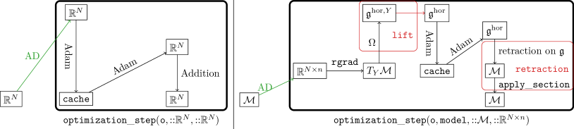
Figure 1: Comparison between regular Adam and Adam adapted to manifolds.

The other mappings, i.e. $\mathtt{update}$ and $\mathtt{velocity}$, as well as the structure of the cache, are however equivalent in both cases. A comparison between those two scenarios is shown in fig. 1.

Algorithm 1 comprises all common first-order optimization algorithms such as (stochastic) gradient descent (with and without momentum) and Adam. The mappings rgrad, lift and retraction, which are needed in addition to the usual steps performed by an optimizer for vector spaces, are now discussed in detail.

Operation 1 (rgrad).

This function computes the Riemannian gradient of a loss function $L$ on a Riemannian matrix manifold $\mathcal{M}\subset\mathbb{R}^{N\times{}n}$ based on its Euclidean gradient $\nabla{}L\in\mathbb{R}^{N\times{}n}$.

For matrix manifolds with Riemannian metric, rgrad can always be found since the Euclidean gradient corresponds to an element of the cotangent space $T_{Y}^{*}\mathcal{M}$ and every element of $T_{Y}^{*}\mathcal{M}$ can be converted to an element of $T_{Y}\mathcal{M}$ with a Riemannian metric $g$ (see [8, Chapter 5]):

$$\langle{}dL,V\rangle\equiv\mathrm{Tr}((\nabla_{Y}L)^{T}V)=g_{Y}(\mathtt{rgrad}(Y,\nabla_{Y}L),V),\quad\forall{}V\in{}T_{Y}\mathcal{M}.$$ (2)

For the Stiefel manifold the canonical metric and the associated gradient are:

$$g_{Y}(V_{1},V_{2})=\mathrm{Tr}\left(V_{1}^{T}\left(\mathbb{I}_{N}-\frac{1}{2}YY^{T}\right)V_{2}\right),$$ (3)

and

$$\mathtt{rgrad}(Y,\nabla{}L)=\nabla{}L-Y\nabla{}L^{T}Y.$$ (4)

How to obtain this canonical metric on $\mathcal{M}$ is discussed in section 3. After we have applied rgrad, we get an element in $T_{Y}\mathcal{M}$. We cannot use this for updating the cache however, since the parametrization of this tangent vector depends on the specific tangent space $T_{Y}\mathcal{M}$. In order to get around this issue we need the notion of a global tangent space representation:

Definition 1 (Global Tangent Space Representation).

A distinct vector space $\mathfrak{g}^{\mathrm{hor}}$ that is isomorphic to $T_{Y}M$ for each $Y\in\mathcal{M}$.

Remark.

Of course every manifold has such a global tangent space representation, because $T_{Y}\mathcal{M}\simeq\mathbb{R}^{d}$ where $d=\mathrm{dim}\mathcal{M}$. But usually the mappings $T_{Y}\mathcal{M}\to\mathbb{R}^{d}$ are very difficult to find. For homogeneous spaces however this is relatively easy (see definition 6).

We can now describe the operation lift in algorithm 1:

Operation 2 (lift).

A mapping from the tangent space $T_{Y}\mathcal{M}$, the output of rgrad, to a global tangent space $\mathfrak{g}^{\mathrm{hor}}$ that is isomorphic to $T_{Y}\mathcal{M}$.

Crucially, every element of the tangent space $T_{Y}\mathcal{M}$, for every $Y\in\mathcal{M}$, can be lifted to $\mathfrak{g}^{\mathrm{hor}}$. Details needed to perform lift are discussed in section 3. For computational purposes lift is performed in two steps as indicated in fig. 1.

Remark.

If $\mathcal{M}$ is a vector space $\mathcal{V}$, then $\mathcal{M}=T_{Y}^{*}\mathcal{M}=T_{Y}\mathcal{M}=\mathfrak{g}^{\mathrm{hor}}=\mathcal{V}$ and no lift is necessary as is the case for the regular Adam algorithm.

In order to define the operation retraction in algorithm 1, we first need the notion of a geodesic.

Definition 2.

A geodesic is the solution of the geodesic differential equation. It is the curve that minimizes the following functional:

$$L(\gamma)=\int_{0}^{1}\sqrt{g_{\gamma(t)}(\dot{\gamma}(t),\dot{\gamma}(t))}.$$

The geodesic differential equation or “geodesic spray” (see [8, chapter 5]) is a second order ordinary differential equation on the manifold $\mathcal{M}$, so takes initial conditions on $T_{Y}\mathcal{M}$. This differential equation can be solved exactly or approximately. In the case in which it is solved approximately, we refer to the approximation as a classical retraction.

Definition 3.

An approximation of the exponential map is referred to as classical retraction and is a map $\mathcal{R}:T\mathcal{M}\to\mathcal{M}$ that satisfies the following two properties: $\mathcal{R}_{Y}(0_{Y})=Y$ and $T_{0_{Y}}\mathcal{R}_{Y}=\mathrm{id}|_{T_{Y}\mathcal{M}}$, i.e. the identity map on $T_{Y}\mathcal{M}$.

Since the Stiefel manifold admits closed-form solutions of its geodesic (see eq. 13), we can use these and do not have to rely on other approximations. Consequently the terms geodesic and retraction will be used interchangeably here.

Remark.

If the considered manifold is a vector space with the canonical metric, the geodesic is simply a straight line: $\gamma(t)=Y+tW$; i.e. the retraction is simple addition in this case (see fig. 1).

For computational purposes the operation retraction in algorithm 1 is different from definition 3, but fulfills the same purpose. For technical reasons its definition is postponed to the next section (see operation 3). Further note that retraction is, analogously to lift, split into two parts. This is indicated in fig. 1.

One can recover the Adam algorithm from algorithm 1 by making the following identifications:

1. The cache in Adam consists of two parameters $\mathcal{B}_{1}^{\mathtt{cache}}$ and $\mathcal{B}_{2}^{\mathtt{cache}}$ for every weight, both of which are elements of $\mathfrak{g}^{\mathrm{hor}}$. They are referred to as the first and second moment.

2. The $\mathtt{cache}=(\mathcal{B}_{1}^{\mathtt{cache}},\mathcal{B}_{2}^{\mathtt{cache}})$ is updated in the following way:

   $$\mathcal{B}_{1}^{\mathtt{cache}}\leftarrow\frac{\beta_{1}-\beta_{1}^{t}}{1-\beta_{1}^{t}}\mathcal{B}_{1}^{\mathtt{cache}}+\frac{1-\beta_{1}}{1-\beta_{1}^{t}}\mathcal{B}_{t},\quad\mathcal{B}_{2}^{\mathtt{cache}}\leftarrow\frac{\beta_{2}-\beta_{2}^{t}}{1-\beta_{2}^{t}}\mathcal{B}_{2}^{\mathtt{cache}}+\frac{1-\beta_{2}}{1-\beta_{2}^{t}}\mathcal{B}_{t}\odot{}\mathcal{B}_{t},$$ (5)

   where $\odot$ is the element-wise Hadamard product, i.e. $(v\odot{}w)_{i}:=v_{i}w_{i}$.

3. For the final velocity:

   $$W_{t}\leftarrow\mathtt{velocity}(\mathtt{cache},\Xi)=-\eta\mathcal{B}^{\mathtt{cache}}_{1}/\sqrt{\mathcal{B}^{\mathtt{cache}}_{2}+\delta},$$ (6)

   where the division $/$ and the addition with the scalar $\delta$ are done element-wise.

The optimization-specific parameters for Adam are $\Xi=(\eta,\beta_{1},\beta_{2},\delta)$. The Adam cache and the Adam operations in equations (5) and (6) are identical for the vector space and the manifold case.

Two related approaches to what is presented here are [25] and [23]. In [25] the authors approximate $\mathcal{B}_{2}^{\mathtt{cache}}$ with a scalar quantity, i.e.

$$\mathcal{B}^{\mathtt{cache}}_{2}\leftarrow\frac{\beta_{2}-\beta_{2}^{t}}{1-\beta_{2}^{t}}\mathcal{B}^{\mathtt{cache}}_{2}+\frac{1-\beta_{2}}{1-\beta_{2}^{t}}||\mathcal{B}_{t}||^{2},$$ (7)

which leads to speed ups in some cases, but ignores the structure of the second moments.

For the case $N=n$, the version of Adam presented in [23] is practically identical to our approach. In this case the global tangent space representation is the collection of skew-symmetric matrices $\mathfrak{g}^{\mathrm{hor}}=\mathfrak{g}=\{\mathcal{B}\in\mathbb{R}^{N\times{}N}:\mathcal{B}^{T}+\mathcal{B}=0\}$. In this case no lift has to be performed. But if $N\neq{}n$, then [23] need a projection, which our algorithm does not need.

In section 4 we compare Adam to two other optimizers: the gradient optimizer and the momentum optimizer which can be derived from the general framework presented in algorithm 1. For these two optimizers:

1. cache is empty; the final velocity $W_{t}$ in algorithm 1 is set to $\mathcal{B}_{t}$ and $\Xi=(\eta)$.

2. cache stores velocity information, i.e. consists of first moments $\mathcal{B}^{\mathtt{cache}}$. This is updated with

   $$\mathcal{B}^{\mathtt{cache}}\leftarrow\alpha\mathcal{B}^{\mathtt{cache}}+\mathcal{B}_{t}.$$ (8)

   The velocity is then computed with $W_{t}\leftarrow\mathtt{velocity(\mathtt{cache},\Xi)}:=-\eta\mathcal{B}^{\mathtt{cache}}$, where $\Xi=(\eta,\alpha)$.

3 Homogeneous Spaces And a Global Tangent Space Representation

In this section we discuss some aspects of homogeneous spaces that are relevant for our algorithm. More extensive treatments can be found in [28, Chapter 11] and [17, Chapter 17]. The Stiefel manifold is used as a concrete example to make abstract constructions more clear, but what is presented here applies to all homogeneous spaces.

Definition 4.

A homogeneous space is a manifold $\mathcal{M}$ on which a Lie group $G$ acts transitively, i.e. the group action $G\times\mathcal{M}\to\mathcal{M}$ is such that $\forall{}Y_{1},Y_{2}\in\mathcal{M}\quad\exists{}\Lambda\in{}G$ s.t. $l_{\Lambda}{}Y_{1}=\Lambda{}Y_{1}=Y_{2}$ (here $l_{\Lambda}$ denotes the left action of an element $\Lambda$ of $G$ onto $\mathcal{M}$).

In the following we will associate a distinct element $E_{\mathcal{M}}\equiv E$ with every homogeneous space $\mathcal{M}$. Because $G$ acts transitively on $\mathcal{M}$, every element of $\mathcal{M}$ can then be represented with an element of $G$ acting on $E$. As an example, consider the orthogonal group $O(N):=\{\lambda\in\mathbb{R}^{N\times{}N}:\lambda^{T}\lambda=\mathbb{I}_{N}\}$ and the Stiefel manifold $\mathcal{M}_{\mathrm{Stiefel}}:=\{Y\in\mathbb{R}^{N\times{}n}:Y^{T}Y=\mathbb{I}_{n}\}$. An element of $O(N)$ is a collection of $N$ orthonormal vectors in $\mathbb{R}^{N}$ and an element of $\mathcal{M}_{\mathrm{Stiefel}}$ is a collection of $n$ orthonormal vectors in $\mathbb{R}^{N}$ where $n<N$. As distinct element for $\mathcal{M}_{\mathrm{Stiefel}}$ we pick:

$$E=\begin{bmatrix}1&0&\ldots&0\\ 0&1&\ldots&0\\ &\ldots&\ldots&\\ 0&0&\ldots&1\\ 0&0&\ldots&0\\ &\ldots&\ldots&\\ 0&0&\ldots&0\end{bmatrix}=\begin{bmatrix}\mathbb{I}_{n}\\ \mathbb{O}\end{bmatrix}\text{, where }\mathbb{O}\in\mathbb{R}^{(N-n)\times{}n}.$$ (9)

If we now apply an element $[y_{1},\ldots,y_{n},y_{n+1},\ldots,y_{N}]=\Lambda\in{}G$ from the left onto $E$, the resulting matrix consists of the first $n$ columns of $\Lambda$: $\Lambda{}E=Y=[y_{1},\ldots,y_{n}]$. So multiplication with $E$ from the right maps $G$ to $\mathcal{M}$. With this we can define the notion of a section:

Definition 5.

A section is a mapping $\lambda:\mathcal{M}\to{}G$ s.t. $\lambda(Y)E=Y$.

Sections are necessary for the computation of lift (see operation 2). We now give a concrete example of a section: Consider the element $Y=[y_{1},y_{2},\ldots,y_{n}]\in\mathcal{M}$. We want to map it to its associated Lie group $G=O(N)$. In order to do so we have to find $(N-n)$ orthonormal vectors that are also orthonormal to $Y$; i.e. we have to find $Q=[q_{1},\ldots,q_{N-n}]$ such that $Y^{T}Q=\mathbb{O}_{n}$ and $Q^{T}Q=\mathbb{I}_{n}$. In the implementation this is done using a $QR$ decomposition (Householder reflections). Details of this are shown in algorithm 2 and further discussed in appendix A.

Algorithm 2 Computation of the lift $Y\mapsto\lambda(Y)\in{}G$ with a $QR$ decomposition.

$A\leftarrow{}\mathcal{P}(\mathbb{R}^{N\times(N-n)})$, $\triangleright$ sample $A$ from a given distribution.

$A\leftarrow A-YY^{T}A$, $\triangleright$ remove the part of $A$ that is spanned by the columns of $Y$.

$Q,R\leftarrow\mathtt{qr}(A)$, $\triangleright$ apply a $QR$ decomposition.

$\lambda(Y)\leftarrow[Y,Q\mathtt{[1:N,1:(N-n)]}]$. $\triangleright$ output $Y$ and the first $(N-n)$ columns of $Q$.

We now proceed with introducing the remaining necessary components that are needed to introduce the global tangent space representation for homogeneous spaces. In the following we assume that the Lie group $G$ is equipped with a Riemannian metric $g$.

First note that $T_{Y}\mathcal{M}\equiv\mathfrak{g}\cdot{}Y$, i.e. the tangent space at $Y$, can be represented by the application of the Lie algebra of $G$ to the element $Y$. The kernel of this map $\mathfrak{g}^{\mathrm{ver},Y}:=\mathrm{ker}(\mathfrak{g}\to{}T_{Y}\mathcal{M})$ is called the vertical component of the Lie algebra at $Y$. Its complement (with respect to the Riemannian metric $g$ on $G$) in $\mathfrak{g}$ is called the horizontal component of $\mathfrak{g}$ at $Y$ and denoted by $\mathfrak{g}^{\mathrm{hor},Y}$; this therefore establishes an isomorphism $\mathfrak{g}^{\mathrm{hor},Y}\simeq{}T_{Y}\mathcal{M}$ and the mapping $\Omega:T_{Y}\mathcal{M}\to\mathfrak{g}^{\mathrm{hor},Y}$ can be found explicitly. For the Stiefel manifold this mapping is:

$$\Omega(\mathtt{rgrad}(Y,\nabla{}L))=\bigg{(}I-\frac{1}{2}YY^{T}\bigg{)}\mathtt{rgrad}(Y,\nabla{}L)Y^{T}-Y(\mathtt{rgrad}(Y,\nabla{}L))^{T}\bigg{(}I-\frac{1}{2}YY^{T}\bigg{)}.$$ (10)

A proof that this indeed established as isomorphism is shown in appendix B. Also see fig. 1 to see where this mapping appears in the algorithm. The mapping $\Omega$ naturally induces a metric on the Stiefel manifold: two vectors of $T_{Y}\mathcal{M}$ can be mapped to $\mathfrak{g}^{\mathrm{hor},Y}\subset\mathfrak{g}$ and the scalar product can be computed in the Lie algebra. If $G=O(N)$ is equipped with the canonical metric one obtains the canonical metric for the Stiefel manifold, presented in equation (3). We can now state a special case of a global tangent space representation as it was defined in definition 1:

Definition 6.

To each homogeneous space we can associate a canonical global tangent space representation $\mathfrak{g}^{\mathrm{hor},E}$ if we have identified a distinct element $E\in\mathcal{M}$. It is the horizontal component of the Lie algebra at the distinct element $E$.

Mapping the output of rgrad (i.e. operation 1), which is an element of $T_{Y}\mathcal{M}$, to the global tangent space representation $\mathfrak{g}^{\mathrm{hor}}$ requires another mapping besides $\Omega:T_{Y}\mathcal{M}\to\mathfrak{g}^{\mathrm{hor},Y}$; one from $\mathfrak{g}^{\mathrm{hor},Y}$ to $\mathfrak{g}^{\mathrm{hor}}\equiv\mathfrak{g}^{\mathrm{hor},E}$. This then completes all the steps required to perform lift (i.e. operation 2).

We obtain this second mapping by first computing a section of $Y$ (see definition 5) and then performing:

$$\Omega(\mathtt{grad}(Y,\nabla{}L))\mapsto\lambda(Y)^{-1}\Omega(\mathtt{grad}(Y,\nabla{}L))\lambda(Y).$$ (11)

The following proposition shows that equation (11) establishes an isomorphism:

Proposition 1.

The map $\mathfrak{g}^{\mathrm{hor},Y}\to\mathfrak{g}^{\mathrm{hor}}$, $Z\mapsto\Lambda^{-1}Z\Lambda$ for any $\Lambda\in{}G$ such that $\Lambda{}E=Y$ is an isomorphism.

Proof.

The considered map is clearly invertible. For the remainder of the proof we have to show that $\Lambda^{-1}Z\Lambda$ is an element of $\mathfrak{g}^{\mathrm{hor}}$ and that for every element $B\in\mathfrak{g}^{\mathrm{hor}}$ there exists $Z_{B}\in\mathfrak{g}^{\mathrm{hor},Y}$ such that $\Lambda^{-1}Z_{B}\Lambda=B$.

For the first part, assume $\Lambda^{-1}Z\Lambda\notin\mathfrak{g}^{\mathrm{hor}}$. This implies that there exists a decomposition $\Lambda^{-1}Z\Lambda=V_{Z}+H_{Z}$ with $V_{Z}\neq 0$ being the vertical part, i.e. $V_{Z}E=0$. But then $Z=\Lambda{}V_{Z}{}\Lambda^{-1}+\Lambda{}H_{Z}\Lambda^{-1}$ with $0\neq\Lambda{}V_{Z}{}\Lambda^{-1}\in\mathfrak{g}^{\mathrm{ver},Y}$. A contradiction.

For the second part, consider $B\in\mathfrak{g}^{\mathrm{hor}}$. By a similar argument as above we can show that $\Lambda{}B\Lambda^{-1}\in\mathfrak{g}^{\mathrm{hor},Y}$. This element fulfills our requirements. ∎

We further note that the particular space $\mathfrak{g}^{\mathrm{hor}}\equiv\mathfrak{g}^{\mathrm{hor},E}$, the horizontal subspace of $\mathfrak{g}$ at $E$, allows for an especially sparse and convenient representation. For the Stiefel manifold:

$$\mathfrak{g}^{\mathrm{hor}}=\left\{\pNiceMatrix[margin=.5em]A&\text{ }-B^{T}\text{ }\\ \text{ }\text{ }\\ B\text{ }0\\ \text{ }\text{ }\CodeAfter\SubMatrix[{1-2}{1-4}]\SubMatrix[{2-1}{4-1}]\UnderBrace[right-shorten,yshift=3pt]{1-1}{4-1}{n}\UnderBrace[left-shorten,yshift=3pt]{1-2}{4-4}{N-n}:A\in\mathbb{R}^{n\times{}n}\text{ is skew-sym, }B\in\mathbb{R}^{N\times(N-n)}\text{ is arbitrary}\right\}.$$ (12)

For fully implementing algorithm 1, we still need a retraction (see operation 3). This equates to finding a geodesic (see definition 2) or an approximation thereof (see definition 3). To do so we utilize the following theorem:

Theorem 1.

Let $\Delta$ be an element of the tangent space $T_{Y}\mathcal{M}$ of a Riemannian homogeneous space $\mathcal{M}$ with Lie group $G$. Then the associated geodesics are $\gamma_{\mathcal{M}}(t;\Delta)=\gamma_{G}(t;\Omega(\Delta))Y$, where $\gamma_{G}$ denotes the geodesic on $G$.

Proof.

See [28, corollary 7.46]. ∎

For $G=O(n)$ the geodesic map $\mathfrak{g}\to{}G$ is just the matrix exponential map. This means that the geodesic for $\Delta\in{}T_{Y}\mathcal{M}$ takes the following form:

$$\gamma_{\mathcal{M}}(t;\Delta)=\gamma_{G}(t;\Omega(\Delta))Y=\exp(t\Omega(\Delta))\lambda(Y)E=\lambda(Y)\exp(t\mathcal{B})E,$$ (13)

where $\mathcal{B}$ is the representation of $\Omega(\Delta)$ in $\mathfrak{g}^{\mathrm{hor}}$, i.e. $\mathcal{B}=\lambda(Y)^{-1}\Omega(\Delta)\lambda(Y)$. It has also been used that $\exp(t\Omega(\Delta))=\exp(t\lambda(Y)\mathcal{B}\lambda(Y)^{-1})=\sum_{n=0}^{\infty}\frac{1}{n!}(t\lambda(Y)\mathcal{B}\lambda(Y)^{-1})^{n}=\lambda(Y)\left(\sum_{n=0}^{\infty}\frac{1}{n!}(t\mathcal{B})^{n}\right)\lambda(Y)^{-1}$. Because of the specific structure of $\mathcal{B}$ (see equation (12)) the computation of the exponential is very cheap (see [4, 18, 16, 12]). This is further discussed in appendix C.

We now finally give the definition of retraction in algorithm 1:

Operation 3 (retraction).

This operation is a map from the global tangent space to the manifold $\mathtt{retraction}:\mathfrak{g}^{\mathrm{hor}}\to\mathcal{M}$ such that $\mathtt{retraction}\circ\Omega:T_{E}\mathcal{M}\to\mathcal{M}$ is a classical retraction according to definition 3 with $\Omega$ being the unique identification $T_{E}\mathcal{M}\to\mathfrak{g}^{\mathrm{hor}}$.

Equation (13) is why the actual computation of the geodesic is split up into two parts, called “retraction on $\mathfrak{g}$” and “apply_section” in fig. 1. The first of these computes $\exp(t\mathcal{B})E$, i.e. is a classical retraction (applied to $\mathcal{B}E\in{}T_{E}\mathcal{M}$) according to definition 3, and the second is the left multiplication by $\lambda(Y)$.

4 Numerical Example: the Transformer

The transformer architecture [31], originally conceived for natural language processing tasks, and the vision transformer [14] (used for processing image data) have largely driven advances in these fields in recent years. Part of the transformer architecture’s allure is that it is a simple and elegant construction that makes the interpretation of the neural network possible, generalizes well to diverse data sets and, perhaps most importantly, its optimization is easily parallelizable which implies good performance on GPUs.

Despite all of this, caution has to be taken when training a transformer network. The original vision transformer paper [14], for example, relies on techniques such as layer normalization [2] and extensive pre-training. Here we demonstrate that this is not necessary when optimizing on the Stiefel manifold; a similar study was performed in [23]. It has also be shown in [32] that weakly-enforced orthogonality constraints, i.e. orthogonality constraints that are added to the loss function via a hyperparameter, are of advantage when dealing with transformers.

The neural networks are trained on the MNIST data set [13]. This data set is split into training and test data; the former consist of 60000 labelled $(28\times 28)$ images and the test data consist of 10000 labelled $(28\times 28)$ images. In order to apply the vision transformer the data are split into 16 $(7\times 7)$ image patches (similar to what was done in [14]), and these collections of 49-dimensional vectors are directly fed into the transformer. The preprocessing steps and the resulting input to the transformer (a $49\times 16$ matrix) are shown in fig. 2. With the terminology used above: $N=49$.

The right part of fig. 2 shows the transformer architecture. At its heart are “multihead attention layers” (introduced in [31]). “Multihead” here refers to the fact that the input is processed multiple times, once for each “head”. Taking as input a matrix $I_{m}\in\mathbb{R}^{49\times 16}$ multihead attention performs the following three computations:

1. Computing three projections (via the matrices $W^{Q}_{i}$, $W^{K}_{i}$ and $W^{V}_{i}$) for each index $i$. The index $i=1,\ldots,7$ indicates the number of the attention head.

2. Weighting the projected “values” $V_{i}:=W^{V}_{i}I_{m}$ by the “queries” $Q_{i}:=W^{Q}_{i}I_{m}$ and the “keys” $K_{i}:=W^{K}_{i}I_{m}$ via an attention mechanism:

   $$\mathtt{Attention}(Q_{i},K_{i},V_{i})=V_{i}\mathrm{softmax}(Q_{i}^{T}K_{i}),$$ (14)

   where the softmax (see appendix D) is computed column-wise.

3. Rearranging the 7 smaller matrices $\in\mathbb{R}^{7\times 16}$ into a bigger one $\in\mathbb{R}^{49\times 16}$ by concatenating them.

So in step (i) the 49-dimensional vectors of the input matrix (see fig. 2) are projected to 7-dimensional vectors with three different projection matrices to obtain “values”, “queries” and “keys”. In step (ii) correlations between the queries and keys are computed via scalar products and these are used to calculate a reweighting of the values. In step (iii) the outputs of the single heads are concatenated so that the multihead attention layer preserves the overall dimension. Also note that the number of heads has to be divisible by $N$ in order to conserve the dimension. The first dimension of the $W_{i}^{(\cdot)}$ matrices is then $n:=N/\mathtt{n\_heads}$.

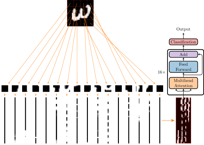
Figure 2: Preprocessing of the images is done in two steps. First the image is split into 16 patches of size $7\times 7$. In the second step the images are flattened and then put together again, yielding a $49\times 16$ matrix. The output is then fed into the transformer.

In our experiments the matrices $W^{Q}_{i}$, $W^{K}_{i}$ and $W^{V}_{i}$ in the multihead-attention layer are constrained to lie on the Stiefel manifold. See appendix E for a further theoretical motivation for this. After applying the multihead attention layer as a preprocessing step, the output is fed into a feedforward neural network with an add connection, i.e.

$$\mathtt{feedforward}:x\mapsto{}x+\sigma(Ax+b).$$ (15)

For this all weights are unconstrained, i.e. $A\in\mathbb{R}^{49\times 49}$ and $b\in\mathbb{R}^{49}$. In our neural network we use 16 such transformer layers. The output of the last transformer is then finally fed into a classification layer that does:

$$\mathtt{classification}:\mathbb{R}^{49\times 16}\to\mathbb{R}^{10},X\mapsto\mathrm{softmax}(WX\mathtt{[1:49,end]}).$$ (16)

This layer takes the last column of the output matrix, multiplies it with a learnable matrix $W\in\mathbb{R}^{10\times{}49}$ and composes it with a softmax.

For the actual training of the transformer we compare four different cases: (i) the transformer with all projection matrices on $\mathbb{R}^{49\times 7}$ and trained with Adam; putting all projection matrices on the Stiefel manifold and optimizing with (ii) gradient descent (iii) gradient descent with momentum and (iv) Adam. The parameters for the various optimizers $\Xi$ are set to the values shown in table 1.

Table 1: Hyperparameters for the various optimizers

Gradient optimizer:	$\eta=0.001$.
Momentum optimizer:	$\eta=0.001$,	$\alpha=0.5$.
Adam optimizer:	$\eta=0.001$,	$\beta_{1}=0.9$,	$\beta_{2}=0.99$,	$\delta=3\cdot 10^{-7}$.

These particular values for the Adam optimizer are typically used as a default and usually do not need much tuning (see [20, chapter 8]). The batch size is set to 2048 and the network is trained for 500 epochs. The data as well as all network parameters are in single precision. For all experiments the regular neural network weights (i.e. the ones in the feedforward neural network and in the classification layer) are initialized with Glorot uniform [19]. The weights that belong to the Stiefel manifold are initialized according to algorithm 3. The probability distributions $\mathcal{P}$ in algorithms 2 and 3 are chosen as products of normal distributions, called with $\mathtt{randn}(N,n)$ in many programming languages.

Algorithm 3 Initializing elements on the Stiefel manifold

$A\leftarrow{}\mathcal{P}(\mathbb{R}^{N\times{}n})$, $\triangleright$ sample $A\in\mathbb{R}^{N\times{}n}$ from a given distribution.

$Q,R\leftarrow\mathtt{qr}(A)$ $\triangleright$ apply a $QR$ decomposition.

$Q\mathtt{[:,1:n]}$ $\triangleright$ output the first $n$ columns of $Q$.

The blue line in fig. 3(a) shows the training of the transformer for which all the weights are in vector spaces (as is usually done); this was called case (i) above. The orange line shows the training for case (iv), i.e. the projections $W^{Q}_{i}$, $W^{K}_{i}$ and $W^{V}_{i}$ in the multi-head attention layer are constrained to lie on the Stiefel manifold. Figure 3(b) shows the difference in training between three optimizers: the standard optimizer (blue, case (ii)), momentum (green, case (iii)) and Adam (orange, case (iv)); we put the weights on the Stiefel manifold in all three cases. The $x$-axis is the epoch and the $y$-axis the training loss.

(a) Training error for Adam optimizers with weights on $\mathbb{R}^{N\times{}n}$ and on $\mathcal{M}$.

(b) Training error for gradient, momentum and Adam optimizers with weights on $\mathcal{M}$.

Figure 3: Training errors for four different optimizers for the problem in fig. 2.

For all of these computations no hyperparameter tuning has been performed. In summary the vision transformer without regularization, dropout or normalization is not able to learn much, as the error rate is stuck at around 1.34, the maximum entropy solution (see appendix D).

As for the comparison of different Stiefel manifold optimizers in fig. 3(b), similar speed-ups are observed as for the Adam optimizer for regular neural networks [22].

We also compare the training times for the four different optimization scenarios shown in fig. 3. The training is performed on CPU (Intel i7-13700K, specified to use 22 cores in parallel) and GPU (Nvidia GeForce RTX 4090). For the GPU implementation we use CUDA.jl (see [7]).

Table 2: Comparison between the times it takes the different optimizers shown in fig. 3 to update the network for the 500 epochs shown.

	Adam	Adam + Stiefel	Gradient + Stiefel	Momentum + Stiefel
GPU	44 minutes	153 minutes	144 minutes	148 minutes
CPU	2783 minutes	2855 minutes	2370 minutes	2369 minutes

Even though GeometricMachineLearning.jl has built-in GPU support, we observe significant performance differences between the Adam optimizer and its Stiefel version (left and right updating scheme in fig. 1). We do not observe this difference if we optimize on the CPU. This is because the AD step(s) in fig. 1 are running completely in parallel on the GPU, whereas the other operations do not. The other operations, necessary for updating the network weights, are very cheap compared to computing the derivative with an AD routine, especially for a big batch size. This is why they do not make the algorithm more expensive in the CPU case; for optimizing on GPU however they become important.

5 Conclusion and Outlook

A generalization of Adam to homogeneous spaces (such as the Stiefel manifold) has been presented. The Adam optimizer for vector spaces can be recovered as a special case.

It has been demonstrated that the resulting optimizers greatly simplify the training of transformer neural networks, as no special techniques like dropout, layer normalization or regularization (and the associated hyperparameter tuning) are needed to achieve convergence. In addition, training the network with manifold structure does not require much more time than training the network without manifold structure on CPU; there is still a relatively large performance gap on GPU however.

Future work will focus on the adaption and implementation of other manifolds and closing the performance gap on GPU by parallelizing the manifold optimizer fully.

Appendix A Computing the Lift $Y\mapsto\lambda(Y)$

The first output of the lift function (i.e. the global section $\lambda$) is computed with a $QR$ decomposition, or more precisely, Householder reflections. These are implemented in most numerical linear algebra libraries.

In essence, Householder reflections take as input an $N\times{}M$ matrix and transform it to an upper-triangular one by a series of $M$ rotations. These rotations are stored in the $Q$ matrix of the $QR$ decomposition.

The computation of the section $\Lambda$ is shown in algorithm 2. The following is needed to ensure $\lambda$ is in fact a lift to $G=O(N)$:

Proposition 2.

Let $Y\in\mathbb{R}^{N\times{}n}$ be a matrix whose columns are orthonormal, $A\in\mathbb{R}^{N\times{}(N-n)}$ be such that $Y^{T}A=\mathbb{O}_{n}$ and $QR=A$ its decomposition. Then $Q^{T}Y=\mathbb{O}_{n}$.

Proof.

Write $Q=[q_{1},\ldots,q_{N-n},\ldots]$. The special structure of $R$ (i.e. $[R]_{ij}=:r_{ij}=0$ for $i>j$) means that the first column of $A=:[a_{1},\ldots,a_{N-n}]$ is a linear combination of $\{q_{1}\}$, the second column is a linear combination of $\{q_{1},q_{2}\}$ and so forth. But this in turn means that every $q_{i}$ ($i=1,\ldots,(N-n$)) can be constructed with columns of $A$. Thus $Q$ and $A$ span the same vector space, and this vector space is orthogonal to $Y$ by assumption. ∎

It should be noted that this specific part of the algorithm is also extendable to, for example, the symplectic Stiefel manifold, as there also exists a Householder routine for this (see [30]). Other $QR$ decompositions may also be used for this step.

Appendix B Induced Isomorphism

The mapping $\Omega$ in equation (10) can be easily shown to established the linear isomorphism $T_{Y}\mathcal{M}\overset{\sim}{\to}\mathfrak{g}^{\mathrm{hor},Y}$:

$$\Omega(\mathtt{rgrad}(Y,\nabla{}L))Y=\bigg{(}I-\frac{1}{2}YY^{T}\bigg{)}\mathtt{rgrad}(Y,\nabla{}L)-\frac{1}{2}Y(\mathtt{rgrad}(Y,\nabla{}L))^{T}Y=\\ \bigg{(}I-\frac{1}{2}YY^{T}\bigg{)}\mathtt{rgrad}(Y,\nabla{}L)+\frac{1}{2}YY^{T}\mathtt{rgrad}(Y,\nabla{}L)=\mathtt{rgrad}(Y,\nabla{}L),$$ (17)

where it was used that $\mathtt{grad}(Y,\nabla{}L)\in{}T_{Y}\mathcal{M}$, i.e. $(\mathtt{grad}(Y,\nabla{}L))^{T}Y=Y^{T}\mathtt{grad}(Y,\nabla{}L)$.

Appendix C Computing Exponentials

As was already discussed by other authors [4, 18, 16, 12], computing the matrix exponential to solve the geodesic in theorem 1 for a matrix manifold with large dimension $N$ and small dimension $n$ only requires computing a matrix exponential of a $2n\times 2n$ dimensional matrix.

The implementation of our algorithm uses the following (also see [12, proposition 3] and [4, proposition 3.8]): The elements of $\mathfrak{g}^{\mathrm{hor}}$ have a special block structure (see equation (12)) that allows each matrix to be written in the following form:

$$\mathfrak{g}^{\mathrm{hor}}=\left\{\begin{bmatrix}\frac{1}{2}A&I\\ B&0\end{bmatrix}\begin{bmatrix}I&0\\ \frac{1}{2}A&-B^{T}\end{bmatrix}:A\in\mathbb{R}^{n\times{}n}\text{ is skew-symmetric, }B\in\mathbb{R}^{N\times{}n}\text{ is arbitrary}\right\}.$$ (18)

The computation of the geodesic can be performed cheaply by recognizing the following (the two block matrices in equation (18) will be called $B^{\prime}$ and $B^{\prime\prime T}$ with $B^{\prime},B^{\prime\prime}\in\mathbb{R}^{N\times 2n}$):

$$\exp(B^{\prime}B^{\prime\prime T})=\sum_{n=0}^{\infty}\frac{1}{n!}(B^{\prime}B^{\prime\prime T})^{n} =I+\sum_{n=1}^{\infty}\frac{1}{n!}B^{\prime}(B^{\prime\prime T}B^{\prime})^{n-1}B^{\prime\prime T}$$ (19)

$$=I+B^{\prime}\left(\sum_{n=1}^{\infty}\frac{1}{n!}(B^{\prime\prime T}B^{\prime})^{n-1}\right)B^{\prime\prime}.$$ (20)

The expression $\mathfrak{A}(B^{\prime},B^{\prime\prime}):=\sum_{n=1}^{\infty}\frac{1}{n!}(B^{\prime\prime T}B^{\prime})^{n-1}$ only involves matrix products of $2n\times 2n$ matrices and can be solved cheaply. To do so we rely on a simple Taylor series expansion:

Algorithm 4 Evaluation of the quantity $\mathfrak{A}(B^{\prime},B^{\prime\prime})\equiv\mathfrak{A}(B^{\prime\prime T}B^{\prime})$.

$\mathtt{output}\leftarrow I$, $\mathtt{product}\leftarrow I$, $t\leftarrow 1$,

while $||\mathtt{product}||<\varepsilon$ do

     $t\leftarrow{}t+1$,

     $\mathtt{product}\leftarrow\frac{1}{t}\mathtt{product*}(B^{\prime\prime T}B^{\prime})$,

     $\mathtt{output}\leftarrow\mathtt{output}+\mathtt{product}$

end while

Here $\varepsilon$ denotes machine precision. With this the retraction takes the form:

$$\mathcal{R}^{\mathrm{geo}}_{Y}(\Delta)\equiv\lambda(Y)\mathtt{retraction}(B)=Y+\lambda(Y)\begin{bmatrix}\frac{1}{2}A&I\\ B&0\end{bmatrix}\mathfrak{A}\left(\begin{bmatrix}\frac{1}{2}A&I\\ \frac{1}{4}A^{2}-B^{T}B&\frac{1}{2}A\end{bmatrix}\right)\begin{bmatrix}I\\ \frac{1}{2}A\end{bmatrix},$$ (21)

where the matrix exponential is now only computed for a small $2n\times 2n$ matrix.

Appendix D The Softmax Activation Function And the Classification Layer

The softmax function maps an arbitrary vector $v\in\mathbb{R}^{\ell}$ to a probability vector $\mathrm{softmax}(v)\in\{w\in(0,1)^{\ell}:\sum_{i=1}^{\ell}{}w_{i}=1\}$ via

$$\mathrm{softmax}(v)=\frac{\exp(v_{i})}{\sum_{i=1}^{\ell}\exp(v_{i})}.$$ (22)

If the output of the softmax is $(\frac{1}{\ell},\ldots,\frac{1}{\ell})$, then we call this the maximum entropy solution. This is what is learned by the network in fig. 2 if we do not constrain the projection matrices to be on the Stiefel manifold. The loss in fig. 3(a) for the case of unconstrained weights is consistently stuck at around 1.34; this is because the output of the network is always $(\frac{1}{10},\ldots,\frac{1}{10})$ and the target is a vector $t\in\{0,1\}^{10}$ with zeros everywhere except for one component. So the resulting $L_{2}$ error is $\sqrt{0.9+9\cdot 0.1}\approx 1.34$.

Appendix E Computing Correlations in the Multihead-Attention Layer

In section 4 multihead attention was described in three steps. Here we elaborate on the second one of these and argue why it makes sense to constrain the projection matrices to be part of the Stiefel manifold.

The attention mechanism in equation (14) describes a reweighting of the “values” $V_{i}$ based on correlations between the “keys” $K_{i}$ and the “queries” $Q_{i}$. First note the structure of these matrices: they are all a collection of 16 7-dimensional vectors, i.e. $V_{i}=[v_{i}^{(1)},\ldots,v_{i}^{(16)}],K_{i}=[k_{i}^{(1)},\ldots,k_{i}^{(16)}]$ and $Q_{i}=[q_{i}^{(1)},\ldots,q_{i}^{(16)}]$ . Those vectors have been obtained by applying the respective projection matrices onto the original image $I_{i}\in\mathbb{R}^{49\times 16}$.

When performing the reweighting of the columns of $V_{i}$ we first compute the correlations between the vectors in $K_{i}$ and in $Q_{i}$ and store the results in a correlation matrix $C_{i}$:

$$[C_{i}]_{mn}=\left(k_{i}^{(m)}\right)^{T}q_{i}^{(n)}.$$ (23)

The columns of this correlation matrix are than rescaled with a softmax function, obtaining a matrix of probability vectors $\mathcal{P}_{i}$:

$$[\mathcal{P}_{i}]_{\bullet{}n}=\mathrm{softmax}([C_{i}]_{\bullet{}n}).$$ (24)

Finally the matrix $\mathcal{P}_{i}$ is multiplied onto $V_{i}$ from the right, resulting in 16 convex combinations of the 16 vectors $v_{i}^{(m)}$ with $m=1,\ldots,16$:

$$V_{i}\mathcal{P}_{i}=\left[\sum_{m=1}^{16}[\mathcal{P}_{i}]_{m1}v_{i}^{(m)},\ldots,\sum_{m=1}^{16}[\mathcal{P}_{i}]_{m16}v_{i}^{(m)}\right].$$ (25)

With this we can now give a better interpretation of what the projection matrices $W_{i}^{V}$, $W_{i}^{K}$ and $W_{i}^{Q}$ should do: they map the original data to lower-dimensional subspaces. We then compute correlations between the representation in the $K$ and in the $Q$ basis and use this correlation to perform a convex reweighting of the vectors in the $V$ basis. These reweighted values are then fed into a standard feedforward neural network.

Because the main task of the $W_{i}^{V}$, $W_{i}^{K}$ and $W_{i}^{Q}$ matrices here is for them to find bases, it makes sense to constrain them onto the Stiefel manifold; they do not and should not have the maximum possible generality.

References

- Absil et al. [2008] P-A Absil, Robert Mahony, and Rodolphe Sepulchre. Optimization algorithms on matrix manifolds. Princeton University Press, Princeton, NJ, 2008.
- Ba et al. [2016] Jimmy Lei Ba, Jamie Ryan Kiros, and Geoffrey E Hinton. Layer normalization. arXiv preprint arXiv:1607.06450, 2016.
- Bécigneul and Ganea [2018] Gary Bécigneul and Octavian-Eugen Ganea. Riemannian adaptive optimization methods. arXiv preprint arXiv:1810.00760, 2018.
- Bendokat and Zimmermann [2021] Thomas Bendokat and Ralf Zimmermann. The real symplectic stiefel and grassmann manifolds: metrics, geodesics and applications. arXiv preprint arXiv:2108.12447, 2021.
- Bendokat and Zimmermann [2022] Thomas Bendokat and Ralf Zimmermann. Geometric optimization for structure-preserving model reduction of hamiltonian systems. IFAC-PapersOnLine, 55(20):457–462, 2022.
- Bendokat et al. [2020] Thomas Bendokat, Ralf Zimmermann, and P-A Absil. A grassmann manifold handbook: Basic geometry and computational aspects. arXiv preprint arXiv:2011.13699, 2020.
- Besard et al. [2018] Tim Besard, Christophe Foket, and Bjorn De Sutter. Effective extensible programming: Unleashing Julia on GPUs. IEEE Transactions on Parallel and Distributed Systems, 2018. ISSN 1045-9219. doi: 10.1109/TPDS.2018.2872064.
- Bishop and Goldberg [1980] Richard L Bishop and Samuel I Goldberg. Tensor analysis on manifolds. Courier Corporation, North Chelmsford, MA, 1980.
- Bolte and Pauwels [2020] Jérôme Bolte and Edouard Pauwels. A mathematical model for automatic differentiation in machine learning. Advances in Neural Information Processing Systems, 33:10809–10819, 2020.
- Brantner and Kraus [2023] Benedikt Brantner and Michael Kraus. Symplectic autoencoders for model reduction of hamiltonian systems. arXiv preprint arXiv:2312.10004, 2023.
- Brantner et al. [2023] Benedikt Brantner, Guillaume de Romemont, Michael Kraus, and Zeyuan Li. Structure-preserving transformers for learning parametrized hamiltonian systems. arXiv preprint arXiv:2312:11166, 2023.
- Celledoni and Iserles [2000] Elena Celledoni and Arieh Iserles. Approximating the exponential from a lie algebra to a lie group. Mathematics of Computation, 69(232):1457–1480, 2000.
- Deng [2012] Li Deng. The mnist database of handwritten digit images for machine learning research. IEEE Signal Processing Magazine, 29(6):141–142, 2012.
- Dosovitskiy et al. [2020] Alexey Dosovitskiy, Lucas Beyer, Alexander Kolesnikov, Dirk Weissenborn, Xiaohua Zhai, Thomas Unterthiner, Mostafa Dehghani, Matthias Minderer, Georg Heigold, Sylvain Gelly, et al. An image is worth 16x16 words: Transformers for image recognition at scale. arXiv preprint arXiv:2010.11929, 2020.
- Duruisseaux and Leok [2022] Valentin Duruisseaux and Melvin Leok. Accelerated optimization on riemannian manifolds via discrete constrained variational integrators. Journal of Nonlinear Science, 32(4):42, 2022.
- Fraikin et al. [2007] Catherine Fraikin, K Hüper, and P Van Dooren. Optimization over the stiefel manifold. In PAMM: Proceedings in Applied Mathematics and Mechanics, volume 7, pages 1062205–1062206. Wiley Online Library, 2007.
- Frankel [2011] Theodore Frankel. The geometry of physics: an introduction. Cambridge university press, Cambridge, England, 2011.
- Gao et al. [2022] Bin Gao, Nguyen Thanh Son, and Tatjana Stykel. Optimization on the symplectic stiefel manifold: Sr decomposition-based retraction and applications. arXiv preprint arXiv:2211.09481, 2022.
- Glorot and Bengio [2010] Xavier Glorot and Yoshua Bengio. Understanding the difficulty of training deep feedforward neural networks. In Yee Whye Teh and Mike Titterington, editors, Proceedings of the Thirteenth International Conference on Artificial Intelligence and Statistics, volume 9 of Proceedings of Machine Learning Research, pages 249–256, Chia Laguna Resort, Sardinia, Italy, 13–15 May 2010. PMLR. URL https://proceedings.mlr.press/v9/glorot10a.html.
- Goodfellow et al. [2016] Ian Goodfellow, Yoshua Bengio, and Aaron Courville. Deep learning. MIT press, Cambridge, MA, 2016.
- Griewank [2003] Andreas Griewank. A mathematical view of automatic differentiation. Acta Numerica, 12:321–398, 2003.
- Kingma and Ba [2014] Diederik P Kingma and Jimmy Ba. Adam: A method for stochastic optimization. arXiv preprint arXiv:1412.6980, 2014.
- Kong et al. [2022] Lingkai Kong, Yuqing Wang, and Molei Tao. Momentum stiefel optimizer, with applications to suitably-orthogonal attention, and optimal transport. arXiv preprint arXiv:2205.14173, 2022.
- Kunstner et al. [2019] Frederik Kunstner, Philipp Hennig, and Lukas Balles. Limitations of the empirical fisher approximation for natural gradient descent. Advances in neural information processing systems, 32, 2019.
- Li et al. [2020] Jun Li, Li Fuxin, and Sinisa Todorovic. Efficient riemannian optimization on the stiefel manifold via the cayley transform. arXiv preprint arXiv:2002.01113, 2020.
- Lin et al. [2023] Wu Lin, Valentin Duruisseaux, Melvin Leok, Frank Nielsen, Mohammad Emtiyaz Khan, and Mark Schmidt. Simplifying momentum-based riemannian submanifold optimization. arXiv preprint arXiv:2302.09738, 2023.
- Mezzadri [2006] Francesco Mezzadri. How to generate random matrices from the classical compact groups. arXiv preprint math-ph/0609050, 2006.
- O’neill [1983] Barrett O’neill. Semi-Riemannian geometry with applications to relativity. Academic press, New York, NY, 1983.
- Raissi et al. [2019] Maziar Raissi, Paris Perdikaris, and George E Karniadakis. Physics-informed neural networks: A deep learning framework for solving forward and inverse problems involving nonlinear partial differential equations. Journal of Computational physics, 378:686–707, 2019.
- Salam et al. [2008] Ahmed Salam, Anas El Farouk, and Eman Al-Aidarous. Symplectic householder transformations for a qr-like decomposition, a geometric and algebraic approaches. Journal of computational and applied mathematics, 214(2):533–548, 2008.
- Vaswani et al. [2017] Ashish Vaswani, Noam Shazeer, Niki Parmar, Jakob Uszkoreit, Llion Jones, Aidan N Gomez, Łukasz Kaiser, and Illia Polosukhin. Attention is all you need. Advances in neural information processing systems, 30, 2017.
- Zhang et al. [2021] Aston Zhang, Alvin Chan, Yi Tay, Jie Fu, Shuohang Wang, Shuai Zhang, Huajie Shao, Shuochao Yao, and Roy Ka-Wei Lee. On orthogonality constraints for transformers. In Proceedings of the 59th Annual Meeting of the Association for Computational Linguistics and the 11th International Joint Conference on Natural Language Processing, volume 2, pages 375–382. Association for Computational Linguistics, 2021.