Distributional Reinforcement Learning with Dual Expectile-Quantile Regression

Abstract

Successful applications of distributional reinforcement learning with quantile regression prompt a natural question: can we use other statistics to represent the distribution of returns? In particular, expectile regression is known to be more efficient than quantile regression for approximating distributions, especially on extreme values, and by providing a straightforward estimator of the mean it is a natural candidate for reinforcement learning. Prior work has answered this question positively in the case of expectiles, with the major caveat that expensive computations must be performed to ensure convergence. In this work, we propose a dual expectile-quantile approach which solves the shortcomings of previous work while leveraging the complementary properties of expectiles and quantiles. Our method outperforms both quantile-based and expectile-based baselines on the MuJoCo continuous control benchmark.

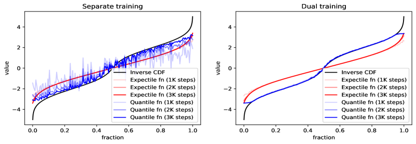
(a) Approximating a distribution with separate and dual training.

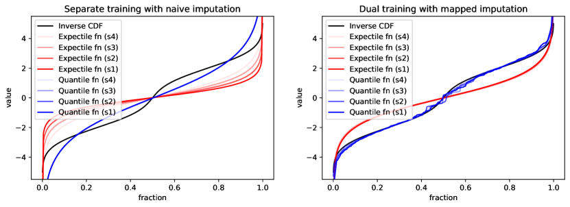
(b) Tabular distributional RL with separate and dual training.

Figure 1: (a) Approximating a bimodal distribution with quantile and expectile regression. Quantile regression approximates the inverse CDF, albeit with high variance, especially on extreme values (left, blue curves). On the other hand, expectiles converge very quickly to the expectile function (left, red curves). However, when training a mapper to generate quantiles from expectiles, quantile estimation becomes much more efficient (right). (b) Distributional RL with function approximation in a chain MDP with 4 states, and a bimodal reward distribution at the last state. The expectile function collapses as the temporal difference error propagates to previous states (left, red curves) while the quantile function is a poor approximation of the inverse CDF (left, blue curves). Our dual method allows to solve both problems (right).

1 Introduction

Distributional reinforcement learning (RL) [3] aims to maintain an estimate of the full distribution of expected return rather than only the mean. It can be used to better capture the uncertainty in the transition matrix of the environment [2], as well as the stochasticity of the policy being evaluated, which may enable faster and more stable training by making better use of the data samples [22].

Non-parametric approximations of the return distribution learned by quantile regression have proven very effective in several domains [7, 8, 37, 17], when combined with deep RL agents such as deep Q-networks (DQN) [24] or soft actor-critic (SAC) [12]. However, quantile-based methods sometimes require an extensive number of steps to outperform the classical agents they are based upon [9], and sometimes fail at solving the task at hand [39]. In this paper, we propose an extension of the non-parametric approach to distributional RL that improves sample efficiency and overall performance. Our approach relies on combining expectile and quantile regression for policy evaluation.

In short, where quantiles are a generalisation of the median, expectiles are a generalisation of the mean. Interestingly, they learn different information about on the distribution: quantiles are trained using an asymmetric L1 loss and are therefore robust to outliers, while expectiles rely on an asymmetric L2 loss, which finds more stable solutions and has better optimization properties. In particular, expectile regression produces the best linear unbiased estimator (BLUE) of any point within the range of the distribution, including all quantiles of the distribution [27]. Moreover, expectile regression provides a straightforward estimator of the mean expected return, i.e., the expectile $0.5$. Finally, expectiles present valuable properties for deep RL that we detail in Section 4. In particular, we show that they allow for an adaptive action selection strategy based on training errors.

The properties listed above make expectile regression a desirable approach for distributional RL. However, in distributional temporal difference learning [3], the distributional Bellman operator requires samples from the target distribution to compute the target during value-function training and, contrary to quantiles, obtaining such samples from expectile values is not obvious. Previous work [30] observed that a naive approach using expectile values as pseudo-samples lacks theoretical guarantees and makes the distribution collapse to the mean in practice. Rowland et al. [30] solved this issue by applying an imputation step that returns samples based on expectile values, and takes the form of finding an approximate solution to an optimization problem. This solution, although effective, is extremely slow, preventing practical applications at scale. Our approach does not have this drawback, as we rely on a dual estimation of quantiles and expectiles, in which quantile values are used to generate samples from the target distribution.

Our contributions can be summarized as follows:

• We propose an implementation of the distributional Bellman operator based on dual estimation of quantiles and expectiles. It solves both in theory and in practice the distribution collapse that previous work observed and does not require intractable computations.

• We show in a toy environment and at scale on continuous control tasks that our proposed operator leads to stronger results than both quantile-based and expectile-based approaches.

• We leverage properties of the expectiles to design an adaptive action selection strategy based on training errors.

• To support the reproducibility of this work, we publicly release the code for our approach.

2 Background

2.1 Distributional reinforcement learning

We consider an environment modeled by a Markov decision process (MDP) $(\mathcal{S},\mathcal{A},R,T,\gamma)$, where $\mathcal{S}$ and $\mathcal{A}$ are a state and action space, respectively, $R(s,a)$ denotes the stochastic reward obtained by taking action $a$ in state $s$, $T(\cdot\mid s,a)$ is the probability distribution over possible next states after taking $a$ in $s$, and $\gamma$ is a discount factor. Furthermore, we write $\pi(\cdot\mid s)$ for a (potentially stochastic) policy selecting the action depending on the current state. We consider the problem of finding a policy maximizing the average discounted return, i.e.,

$$\pi^{*}=\arg\max_{\pi}\mathbb{E}\left[\sum_{t=0}^{\infty}\gamma^{t}R(s_{t},a_{t})\right],$$ (1)

where $a_{t}\sim\pi(\cdot\mid s_{t})$ and $s_{t+1}\sim T(\cdot\mid s_{t},a_{t})$. We can define the action-value random variable for policy $\pi$ as $Z^{\pi}:(s,a)\mapsto\sum_{t=0}^{\infty}\gamma^{t}R(s_{t},a_{t})$, with $s_{0}=s,a_{0}=a$. We will refer to action-value variables as $Z$-functions in the remainder. Note that the $Q$-function, as usually defined in RL [33], is given by $Q^{\pi}(s,a)=\mathbb{E}\left[Z^{\pi}(s,a)\right]$. In this work, we consider approaches that evaluate policies through distributional dynamic programming, i.e., by repeatedly applying the distributional Bellman operator $\mathcal{T}$ to a candidate $Z$-function:

$$\mathcal{T}Z(s_{t},a_{t})=R(s_{t},a_{t})+\gamma Z(s_{t+1},a_{t+1}).$$ (2)

This operator has been shown to be a contraction in the $p$-Wasserstein distance and therefore admits a unique fixed point $Z^{\pi}$ [2]. A major challenge of distributional RL resides in the choice of representation for the action-value distribution, as well as the exact implementation of the distributional Bellman operator.

2.2 Quantile and expectile regression

Let $Z$ be a real-valued probability distribution. The $\alpha$-quantile $q_{\alpha}$ of $Z$ is defined as a value splitting the probability mass of $Z$ in two parts of weights $\alpha$ and $1-\alpha$, respectively:

$$P(z\leq q_{\alpha})=\alpha.$$ (3)

Therefore, the quantile function $\mathcal{Q}_{Z}:\alpha\mapsto q_{\alpha}$ is the inverse cumulative distribution function: $\mathcal{Q}_{Z}=F_{Z}^{-1}$. Alternatively, quantiles are given by the minimizer of an asymmetric $L_{1}$ loss:

$$q_{\alpha}=\arg\min_{q}\mathbb{E}_{z\sim Z}\left[\left(\alpha\mathds{1}_{z>q}+(1-\alpha)\mathds{1}_{z\leq q}\right)\left|z-q\right|\right].$$ (4)

Expectiles and the expectile function $\mathcal{E}_{Z}:\tau\mapsto e_{\tau}$ are defined analogously, as the $\tau$-expectile $e_{\tau}$ minimizes the asymmetric $L_{2}$ loss:

$$e_{\tau}=\arg\min_{e}\mathbb{E}_{z\sim Z}\left[\left(\tau\mathds{1}_{z>e}+(1-\tau)\mathds{1}_{z\leq e}\right)\left(z-e\right)^{2}\right].$$ (5)

Furthermore, while Eq. 3 characterizes quantiles using a condition on probability mass, the expectiles are characterized by a partial moment condition:

$$\tau\int_{e_{\tau}}^{\infty}(z-e_{\tau})dz=(1-\tau)\int_{-\infty}^{e_{\tau}}(e_{\tau}-z)dz.$$ (6)

In particular, the median is the $0.5$-quantile and the mean is the $0.5$-expectile. A consequence is that expectile regression provides a straightforward estimator of the mean return in RL, while the (weighted) mean of quantiles has been used to approximate the mean in previous work on distributional RL with quantile regression [7, 8, 37], even though this estimator is biased when approximating a finite number of quantiles.

As mentioned in the introduction, the $L_{1}$ and $L_{2}$ losses used in quantile and expectile regression, respectively, possess different properties. The $L_{1}$ loss is more robust to outliers [15] while the $L_{2}$ loss provides more stable solutions, as it is continuously differentiable. Interestingly, expectile regression provides the best linear unbiased estimator of any location parameter within the range of the data distribution, including all quantiles [27]. This suggests that equipped with the right tools, expectile regression can give better approximation of the quantiles than quantile regression itself. This idea motivates our dual approach, and we verify this property on a toy example in Section 5.1.

Expectiles possess several other interesting properties, as detailed in [28], some of which we use in our method in Section 4.

2.3 Naive expectile-based distributional RL suffers from target mismatch

Quantile regression has been used for distributional RL in many previous studies [7, 8, 37] where a parameterized quantile function $\mathcal{Q}_{Z}^{\theta}(s,a,\alpha)$ is trained using a quantile temporal difference loss function derived from Eq. 4:

$$\mbox{}\mathcal{L}_{\mathcal{Q}}\left(\mathcal{Q}_{Z}^{\theta}(s,a,\cdot)\right)\!=\!\sum_{i=1}^{N}\sum_{j=1}^{N}l_{\mathcal{Q}}(q_{i},z_{j})\textup{ with }l_{\mathcal{Q}}(q_{i},z_{j})\!=\!\left(\alpha_{i}\mathds{1}_{z_{j}>q_{i}}+(1-\alpha_{i})\mathds{1}_{z_{j}\leq q_{i}}\right)\left|z_{j}-q_{i}\right|,\mbox{}$$ (7)

where the trainable quantile values $q_{i}=\mathcal{Q}_{Z}^{\theta}(s,a,\alpha_{i})$ are obtained by querying the quantile function at various quantile fractions $\alpha_{i}$, which can be fixed by the designer [8], sampled from a distribution [7], or learned during training [37]. In quantile-based temporal difference (QTD), the target samples $z_{j}$ can be obtained by querying the estimated quantile function at the next state-action pair: $z_{j}=r+\gamma\mathcal{Q}_{Z}^{\theta}(s^{\prime},a^{\prime},\alpha_{j})$. Indeed, because the true quantile function is the inverse CDF of the action-value distribution, Dabney et al. [8] and Bellemare et al. [3] showed that quantiles at equidistant fractions minimize the $1$-Wasserstein distance with the action-value distribution and that the resulting projected Bellman operator is a contraction mapping in such a distance. Rowland et al. [31] extended these results to prove the convergence of QTD learning under mild assumptions. We refer to these studies for a more detailed convergence analysis.

In contrast, expectile-based temporal difference (ETD) does not allow the same update rule as the one given by Eq. 7. We first write the generic ETD loss derived from Eq. 5:

$$\mbox{}\mathcal{L}_{\mathcal{E}}\left(\mathcal{E}_{Z}^{\theta}(s,a,\cdot)\right)\!=\!\sum_{i=1}^{N}\sum_{j=1}^{N}l_{\mathcal{E}}(e_{i},z_{j})\textup{ with }l_{\mathcal{E}}(e_{i},z_{j})=\left(\tau_{i}\mathds{1}_{z_{j}>e_{i}}+(1-\tau_{i})\mathds{1}_{z_{j}\leq e_{i}}\right)\left(z_{j}-e_{i}\right)^{2},\mbox{}$$ (8)

with $e_{i}=\mathcal{E}_{Z}^{\theta}(s,a,\tau_{i})$. Here, choosing $z_{j}=r+\gamma\mathcal{E}_{Z}^{\theta}(s^{\prime},a^{\prime},\tau_{j})$, analogously to QTD and non-distributional TD, would cause the update to approximate a different distribution because the expectile function is in general not the inverse CDF of the return distribution. Rowland et al. [30] formalized this idea using the concept of Bellman closedness, i.e., that the Bellman operator yields the same statistics whether it is applied to the target distribution or to the implicit distribution given by statistics of the target distribution (i.e., in our case a mixture of diracs with locations given by quantiles or expectiles). They showed that quantiles are approximately Bellman closed, while expectiles are not.

In practice, one may observe that with the naive approach, every estimated expectile collapses to the mean after multiple updates [30], as we can show that, e.g., the expectile function of a Gaussian distribution is another Gaussian distribution with the same mean and a strictly lower variance [28]. Rowland et al. [30] yield a well-behaved update by adding an imputation step that consists in generating samples $z_{j}$ of the target distribution from estimated expectiles $e_{j}$, which requires solving a root-finding problem. This approach becomes extremely slow as we increase the number of estimated expectiles, rendering it unusable at scale.

3 Related Work

3.1 Distributional RL

Distributional reinforcement learning aims to approximate the distribution of future returns $Z$, instead of its expectation $Q$. This results in several benefits – by ascribing randomness to the value of a state-action pair, an algorithm can learn more efficiently for close states and actions [22], as well as capture possible stochasticity in the environment [21].

Estimating a parameterized distribution is a straightforward approach, and has been mostly explored from both Bayesian [32, 35] and frequentist [17] perspectives. However, this usually requires an expensive likelihood computation, as well as making a restrictive assumption on the shape of the distribution $Z$. For instance, assuming a normal distribution when the actual distribution is heavy-tailed can yield disappointing results.

Thus, non-parametric approaches are also used to approximate the distribution. C51 [2] quantizes the domain where $Z$ has a non-zero density (usually in 51 atoms, hence the name), and performs weighted classification on the atoms, by computing the cross-entropy between $Z$ and $\mathcal{T}Z$. While C51 greatly increases performance over a deterministic evaluation of the $Q$-value, it requires the user to set the bounds of the divided interval, does not have a proper distribution structure, and relies on averaging the mass points to obtain an estimation of the mean. Yet, biased estimation of the mean of a distribution is likely to deteriorate the average performance [23]. Other work optimizes on risk metrics such as Value-at-Risk directly, in order to promote exploration safety or prevent risky outcomes [6, 22, 18].

Another important non-parametric approach to the estimation of a distribution is quantile regression. Quantile regression originally relies on the minimization of an asymmetric $L1$ loss. Estimating the quantiles of a distribution allows to approximate the action-value distribution without relying on a shape assumption. QR-DQN [8] introduced quantile regression as a way to minimize the earth mover’s distance (or Wasserstein loss) between $Z$ and $\mathcal{T}Z$. Further, implicit quantile networks (IQN) [7] embed the quantile fraction, in order to process it in the Q-network of a DQN algorithm. Fully parameterized quantile functions (FQF) [37] additionally learn the optimal quantile fractions, that are then used to compute the values via IQN’s embeddings. However, none of the work above addresses the problem of quantile crossing: the value of the quantile 0.2 should be inferior to the value of the quantile 0.3, to respect the monotonicity of the Cumulative Density Function of $Z$ [13].

3.2 Expectile regression

Expectiles were originally introduced as a family of estimators of location parameters for a given distribution, to palliate possible heteroskedasticity of the error terms in regression [25, 27].

Expectiles can be seen as mean estimators under missing data [28]. Unlike quantiles, they span the entire convex hull of the distribution’s support, and on this ensemble, the expectile function is strictly increasing: an expectile fraction is always associated to a unique value. Expectiles have been used in reinforcement learning successfully before [30], but in a way that requires a slow optimization step to achieve satisfactory performance. Moreover, expectile regression is subject to the same crossing issue as quantiles, albeit empirically less so [36]. Expectiles have also been used in offline reinforcement learning to compute a soft maximum over potential outcomes seen in the offline data [19].

In this paper, we make use of the relation between quantiles and expectiles to learn both at the same time, circumventing the theoretical weaknesses of both approaches. Moreover, our use of monotonically increasing neural networks ensures that neither quantile or expectile curves cross.

4 Method

4.1 Training expectiles and quantiles together

We propose to train a single parameterized $Z$-function using both quantile and expectile regression. We first note that the expectile function at a given state-action pair $\mathcal{E}_{Z(s,a)}:[0,1]\rightarrow\mathbb{R}$ is a strictly increasing function that spans the entire convex hull of the distribution’s support. On the other hand, the quantile function $\mathcal{Q}_{Z(s,a)}:[0,1]\rightarrow\mathbb{R}$ is non-decreasing and spans the distribution’s support. As a consequence, there exists a strictly increasing functional mapping from quantiles to expectiles. In this work, we propose to train a mapper $\mathcal{M}:[0,1]\rightarrow[0,1]$ to approximate a mapping between quantile fractions and corresponding expectile fractions. In other words, we want $\mathcal{Q}_{Z(s,a)}\left(\tau\right)=\mathcal{E}_{Z(s,a)}(\mathcal{M}(\tau))$.

Yao and Tong [38] show that for regression with a location-scale model, quantile and expectile functions share the same feature-dependent parameters:

$$\mathcal{Q}_{Z\mid X}(\tau)=\mu(X)+\sigma(X)\mathcal{Q}_{\epsilon}(\tau)\;\textup{ and }\;\mathcal{E}_{Z\mid X}(\tau)=\mu(X)+\sigma(X)\mathcal{E}_{\epsilon}(\tau),$$ (9)

where $\epsilon$ defines the shape of the distribution, $\mu$ the location and $\sigma$ the scale. As a consequence, under this model, the quantile-to-expectile mapper is independent of the state-action pair $X$, and we can write:

$$\forall s\in\mathcal{S},a\in\mathcal{A},\tau\in[0,1]\;\mathcal{Q}_{Z(s,a)}\left(\tau\right)=\mathcal{E}_{Z(s,a)}(\mathcal{M}_{Z}(\tau)).$$ (10)

Motivated by these properties, we design a practical implementation of Eq. 10 for temporal difference using a parameterized function $S_{\theta}^{s,a}(\tau)$ and a parameterized mapper $m_{\phi}(\tau)$, in order to approximate the expectiles and quantiles of $Z(s,a)$. Following Dabney et al. [7], we sample uniformly in $[0,1]$ a set of fractions $\tau_{1},\dots,\tau_{N}$ at each training step. The expectile loss from Eq. 5 is used to train $\theta$, while the quantile loss from Eq. 4 is used to train both $\theta$ and $\phi$, that is, given a tuple of experience $(s,a,r,s^{\prime},a^{\prime})$:

$$\begin{split}\mathcal{L}^{\theta,\phi}(s,a)&=\mathcal{L}_{\mathcal{E}}(S_{\theta}^{s,a}(\tau))+\mathcal{L}_{\mathcal{Q}}\left(S_{\theta}^{s,a}(m_{\phi}(\tau))\right)\\ &=\sum_{i=1}^{N}\sum_{j=1}^{N}\left(\tau_{i}\mathds{1}_{z_{j}>S_{\theta}^{s,a}(\tau_{i})}+(1-\tau_{i})\mathds{1}_{z_{j}\leq S_{\theta}^{s,a}(\tau_{i})}\right)\left(z_{j}-S_{\theta}^{s,a}(\tau_{i})\right)^{2}\\ &\;\;\;\;+\left(\tau_{i}\mathds{1}_{z_{j}>S_{\theta}^{s,a}(m_{\phi}(\tau_{i}))}+(1-\tau_{i})\mathds{1}_{z_{j}\leq S_{\theta}^{s,a}(m_{\phi}(\tau_{i}))}\right)\left|z_{j}-S_{\theta}^{s,a}(m_{\phi}(\tau_{i}))\right|.\end{split}$$ (11)

As we recalled in Section 2, the way we generate samples $z_{j}$ from the target distribution is crucial in distributional RL. While Rowland et al. [30] resorted to solving a root-finding problem at each training step, we can simply query our estimator of quantiles at the next state-action pair to yield a sound imputation step:

$$\forall j\in{1,\dots,N},\;z_{j}=r+\gamma\cdot\mathrm{stop\_grad}\left(S_{\theta}^{s^{\prime},a^{\prime}}(m_{\phi}(\tau_{j}))\right).$$ (12)

We refer to the algorithm based on the update described in Eqn. 11 and 12 as expectile-quantile temporal difference (EQTD), and provide pseudo-code of its value function update in Algorithm 1.

Algorithm 1 Expectile-quantile temporal difference (EQTD) update pseudo-code

Statistic function $S_{\theta}$, mapper $m_{\phi}$, fractions $(\tau_{i})_{i=1,\dots,N}$, learning rate $\eta$.

Collect experience $(s,a,r,s^{\prime},a^{\prime})$

for $i=1,\dots,N$ do

     Compute expectile values $e_{i}\leftarrow S_{\theta}(s,a,\tau_{i})$ and quantile values $q_{i}\leftarrow S_{\theta}(s,a,m_{\phi}(\tau_{i}))$

     Compute target samples $z_{i}\leftarrow r+\gamma\cdot\mathrm{stop\_grad}(S_{\theta}(s^{\prime},a^{\prime},\alpha_{i}))$

end for

for $i=1,\dots,N$ do

     Compute expectile loss $\mathcal{L}_{\mathcal{E}}\leftarrow\frac{1}{N}\sum_{j=1}^{N}\left(\tau_{i}\mathds{1}_{z_{j}>e_{i}}+(1-\tau_{i})\mathds{1}_{z_{j}\leq e_{i}}\right)\left(z_{j}-e_{i}\right)^{2}$

     Compute quantile loss $\mathcal{L}_{\mathcal{Q}}\leftarrow\frac{1}{N}\sum_{j=1}^{N}\left(\tau_{i}\mathds{1}_{z_{j}>q_{i}}+(1-\tau_{i})\mathds{1}_{z_{j}\leq q_{i}}\right)\left|z_{j}-q_{i}\right|$

     Update statistic function parameters $\theta\leftarrow\theta-\eta\nabla_{\theta}\mathcal{L}_{\mathcal{E}}$

     Update mapper parameters $\phi\leftarrow\phi-\eta\nabla_{\phi}\mathcal{L}_{\mathcal{Q}}$

end for

4.2 Action selection strategy for environment interactions

This section is concerned with the choice of statistic to be considered by the agent when interacting with the environment. Previous studies based on quantiles have considered the CVaR [20] or the (potentially weighted) mean of quantiles [8, 37], and previous work on expectile-based distributional RL used the expectile $0.5$ [30], as it is a natural estimator of the mean. We take a different approach by leveraging properties of the expectiles. Namely, expectile regression offers the possibility of adapting the action selection strategy, even when our goal is to optimize for the mean return. This allows us to propose a method allowing faster propagation of the temporal difference error and, as a result, better sample-efficiency.

Given a tuple of experience $(s,a,r,s^{\prime},a^{\prime})$, we write $\epsilon^{\tau}=S_{\theta}^{s,a}(\tau)-(r+\gamma z^{\prime})$ for the distributional TD error for a fixed $\tau$ with $r\sim R$ and $z^{\prime}\sim Z(s^{\prime},a^{\prime})$, and we define $\epsilon:=\epsilon^{0.5}$. Ideally, after training, we should have $\mathbb{E}\left[\epsilon\right]=0$. However, it is likely that during training, we have $\mathbb{E}\left[\epsilon\right]\neq 0$, as the policy being evaluated has not been fully fitted yet. Thus, acting greedily with respect to the mean may be suboptimal, therefore hurting exploitation.

Expectiles offer the opportunity to act optimally even if the TD error has not been fully reduced yet, by acting greedily with respect to a different expectile $\tau^{\mathrm{act}}$, such that $\mathbb{E}[\epsilon^{\tau^{\mathrm{act}}}]=0$. An interesting property of expectiles is that the expectile indexed by $\tau$ corresponds to the mean of a particular reweighted regression problem, where values above it are rescaled by a factor $\tau$ and values below by a factor $1-\tau$ [28]. Therefore, to obtain the formula for $\tau^{\mathrm{act}}$, we can first write:

$$\mathbb{E}[\epsilon^{\tau}]=\tau\mathbb{E}[\,\epsilon\mid\epsilon\geq 0]\mathrm{Pr}(\epsilon\geq 0)+(1-\tau)\mathbb{E}[\,\epsilon\mid\epsilon<0]\mathrm{Pr}(\epsilon<0).$$ (13)

Then the rescaled error $\epsilon^{\tau^{\mathrm{act}}}$ is centered on $0$ if $\mathbb{E}[\epsilon^{\tau^{\mathrm{act}}}]=0$, i.e.,

$$\tau^{\mathrm{act}}\mathbb{E}[\,|\epsilon|\mid\epsilon\geq 0]\mathrm{Pr}(\epsilon\geq 0)=(1-\tau^{\mathrm{act}})\mathbb{E}[\,|\epsilon|\mid\epsilon<0]\mathrm{Pr}(\epsilon<0),$$ (14)

which, assuming $\epsilon\neq 0$, gives a formula for the selection of $\tau^{\mathrm{act}}$:

$$\tau^{\mathrm{act}}=\frac{1}{1+\frac{\mathbb{E}[\,|\epsilon|\mid\epsilon\geq 0]\mathrm{Pr}(\epsilon\geq 0)}{\mathbb{E}[\,|\epsilon|\mid\epsilon<0]\mathrm{Pr}(\epsilon<0)}}.$$ (15)

In practice, given a batch of training errors $\epsilon$, we compute empirically the expectile fraction $\tau^{\mathrm{act}}$ and use it to act in the environment. In our case, we use soft actor-critic (SAC) [12] as the backbone for our method, so we train the actor on the task of maximizing the corresponding expectile value of the $Z$-function, that is, given an actor $\pi_{\psi}$ parameterized by $\psi$ and a parameter $\alpha$ controlling the entropy of the desired policy, we maximize the following loss by gradient ascent:

$$\mathcal{L}^{\psi}(s,a)=S_{\theta}(s,a_{\psi},\tau^{\mathrm{act}})-\alpha\log\pi_{\psi}(a_{\psi}\mid s),\textup{ with }a_{\psi}\sim\pi_{\psi}(\cdot\mid s).$$ (16)

For better robustness, we perform a soft update of $\tau^{\mathrm{act}}$ at each training step by Polyak averaging [29] with the same forgetting factor as for target networks of the $Z$-function. Also, we noticed in our experiments that individual errors could be very large and challenge the stability of our agent, so we clip $\mathbb{E}[\,|\epsilon|\mid\epsilon\geq 0]$ and $\mathbb{E}[\,|\epsilon|\mid\epsilon\geq 0]$ in Eq. 15. We perform an ablation study in Appendix B.

4.3 Implementation details

4.3.1 Baselines

We experimented with the following baselines to evaluate our approach:

• Soft actor-critic (SAC): We take the SAC implementation provided by CleanRL [16], and further tune it to ensure a fair comparison. In particular, we added layer normalization to the Q-network as it gives stronger results, in line with recent research [14, 1], and re-ran the hyperparameter search.

• Quantile temporal difference (QTD): We approximate quantiles using the general approach described in IQN [7], on top of the SAC method described above, with minor modifications detailed in the next section.

• Expectile temporal difference (ETD): We use a similar approach as for QTD, but trained with an expectile loss and a naive imputation step as described in [30], i.e., expectile values are used as target for the temporal difference loss.

4.3.2 Network architectures and hyperparameters

We base all baselines and our method on the same underlying neural network, derived from CleanRL’s implementation of SAC [16]. Hyperparameters can be found in Appendix A.

For distributional methods, we implemented the $Z$-function as a feed-forward neural network where weights relating to the statistic fraction are forced to be positive, in order to ensure monotonicity of the quantile and expectile functions and prevent quantile crossings [13]. We did not use the fraction proposal network introduced with FQF [37], as well as the sinusoidal embeddings proposed by IQN [7], as they did not lead to any significant improvement. Finally, we found that using layer normalization increased performance for both our method and baselines. Similarly to previous quantile-based methods, we use the $N=200$ statistics sampled at each training step to generate $N$ samples from the target distribution.

The mapper is implemented as a monotonic neural network. To do so, we simply force its weights to be positive, and process the output through a sigmoid function to constrain the output between 0 and 1. Since the mapper is queried to obtain both the candidate and target values, we use a mapper-specific target network updated less frequently than the live network, using Polyak averaging [29].

5 Experiments

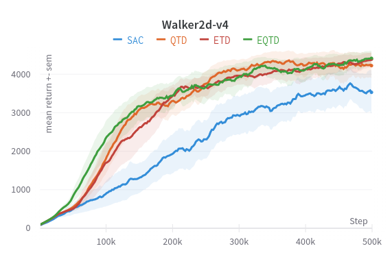
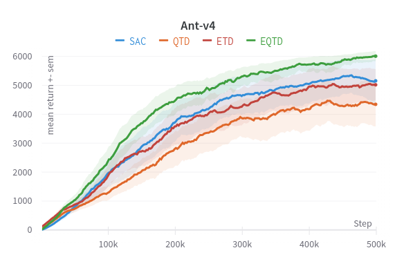
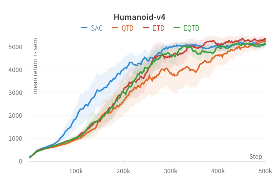
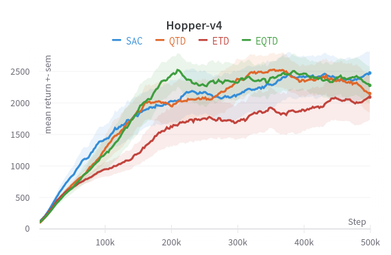
Figure 2: Average return of $5$ seeds on the MuJoCo continuous control benchmark.

5.1 Chain MDP: A toy example

We start by observing the effect of our proposed operator in a toy environment. The MDP comprises $4$ states, with each state pointing to the next through a unique action and without accumulating any reward, until the agent reaches the last state $s_{4}$, where the episode terminates and the agent obtains a reward sampled from a bimodal distribution $r\sim\left(\frac{1}{2}\mathcal{N}(-2,1)+\frac{1}{2}\mathcal{N}(+2,1)\right)$. A visual description of the MDP is given in Appendix C.

Figure 1(a) highlights the advantageous properties of expectile regression that were introduced in prior work [27, 28, 38, 36]. When trying to approximate the distribution of terminal rewards directly from samples (left plot), expectile regression yields more accurate estimates than quantile regression in the low-data regime (recall that the quantile function is the inverse CDF while the expectile function is in general not). Interestingly, the right plot shows that coupling expectile regression with our mapper allows us to recover the quantile function much more efficiently than quantile regression itself!

In Figure 1(b) (left), we illustrate the deficiencies of regular QTD and ETD. QTD is sample-inefficient and fails to approximate the distribution within the given evaluation budget. However, we observe that the distribution information is propagated correctly through temporal difference updates, since the quantile functions estimated at each state coincide. On the contrary, the expectile function collapses to the mean as the error propagates from $s_{4}$ to $s_{1}$. This is due to the fact that expectile values at the next state-action pair cannot be used as pseudo-samples of the return distribution $Z(s^{\prime},a^{\prime})$ [30] .

Finally, Figure 1(b) (right) shows that our dual training method, where the pseudo-samples of $Z(s^{\prime},a^{\prime})$ are the estimated quantiles $S_{\theta}^{s^{\prime},a^{\prime}}(m_{\phi}(\tau))$, solves both issues: the expectile function does not collapse anymore and the quantile function approximation is more accurate.

5.2 MuJoCo: Continuous control with stochastic policies

In this section, we verify that our dual approach also provides benefits at scale, on continuous control environments. We opted for the MuJoCo control benchmark [34], and in particular the set of Gymnasium [11] environments considered in previous work on SAC-based agents [14, 5]: Ant-v4, Hopper-v4, Humanoid-v4, and Walker2d-v4. We train all agents for a total of $500$ thousand environment steps, and plot the average return. We repeat this process for 5 different seeds, in order to reduce the uncertainty of our results. The results of our experiments can be found in Figure 3.

A first observation is that a well-tuned SAC agent is a hard baseline to beat, even for distributional approaches. While distributional approaches clearly beat SAC on Walker2d, they perform similarly or sometimes worse on other environments. However, our dual approach always performs similarly or better than distributional baselines, beats all baselines on Ant, and is the most sample-efficient approach on Hopper and Walker2d. In particular, our dual EQTD approach retains a strong performance when either QTD or ETD fail, suggesting it gets the best of both worlds, as shown in the toy environment.

6 Limitations and broader impact

Limitations. Our method implies that the action-value distribution follows a distribution from the location-scale family (Eq. 9). While this seems limiting, it does not require all states to be allocated the same distributions, only that the mapping between them remains the same. Moreover, the location-scale family is quite broad, as it includes Normal, Student, Cauchy, GEV distributions, and more. More experiments in various environments would be needed to test the robustness of this assumption. Finally, while our method adds limited overhead to distributional baselines compared to previous work [30], it is still slower than a simple SAC baseline.

Broader impact statement. Automated decision making, when employed in resource allocation, has the potential to discriminate populations based on various factors [10] – this is even more true for minorities, that are often not present enough in the training of such algorithms [4]. While this drawback is present in most applications of RL, we believe that moving towards distributional reinforcement learning helps in accounting for edge cases. This is even more true with expectiles, that are notoriously good at representing threshold effects and outliers [27].

7 Conclusion

We proposed a non-parametric approach to distributional reinforcement learning based on the simultaneous estimation of quantiles and expectiles of the action-value distribution. This approach presents the advantage of leveraging the efficiency of the expectile-based loss for both expectile and quantile estimation while solving the theoretical shortcomings of expectile-based distributional reinforcement learning, which tends to lead to a collapse of the expectile function in practice.

We showed on a toy environment how the dual optimization affects the statistics recovered in distributional RL: in short, the quantile function is estimated more accurately than with vanilla quantile regression and the expectile function remains consistent after several steps of temporal difference training. We then assessed the performance of the dual expectile-quantile temporal difference (EQTD) at scale, on the MuJoCo benchmark. Our agent surpassed the performance of both expectile and quantile-based agents, demonstrating its effectiveness in practical scenarios.

For future work, we plan to investigate how the dual EQTD approach can be used in risk-aware decision-making problems, and how it performs when the goal is to minimize risk metrics such as (conditional) value-at-risk. Moreover, we plan to gather insights into what type of behavior is favored by the quantile and expectile loss, respectively.

Appendix

Appendix A Hyperparameters and training setup

We use Pytorch [26] to train our models on a single gpu (NVIDIA A100 80GB). A full training procedure of $500$K training steps and corresponding validation steps takes approximately $6$ hours in our setup.

Key	Value
Discount factor	$0.99$
Batch size	$256$
Actor learning rate	$3\mathrm{e}^{-4}$
Critic learning rate	$1\mathrm{e}^{-3}$
Entropy learning rate	$1\mathrm{e}^{-3}$
Random steps before training	$5000$
Size of hidden layer	$512$
Critic updates per sample	$2$
Samples between actor updates	$2$
Samples between target network updates	$2$
Target network update rate	$0.5$
Variance of exploration noise	$0.1$
Exploration noise clipping	$0.5$

Table 1: Shared hyperparameters

Key	Value
Number of statistics	$200$
Number of samples for critic update	$200$
Fraction distribution	$\mathcal{U}([0,1])$
Magnitude ratio clipping (ETD, EQTD)	$1$
Weight of quantile loss (EQTD)	$5$
Mapper learning rate (EQTD)	$1\mathrm{e}^{-3}$
Target mapper update rate (EQTD)	$5\mathrm{e}^{-4}$

Table 2: Distributional hyperparameters

Appendix B Ablation study for the action selection strategy

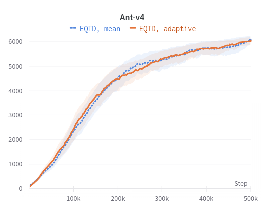
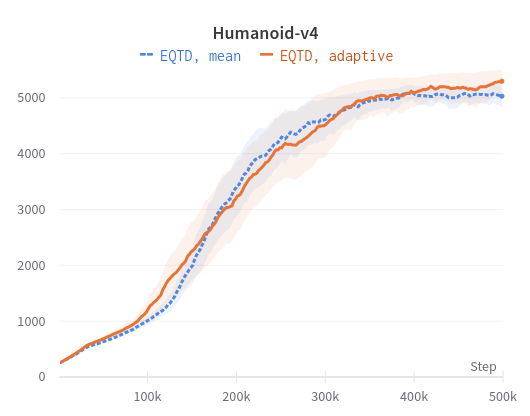
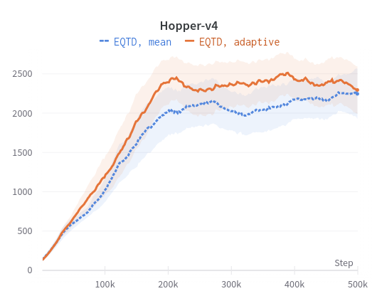
Figure 3: Ablation study of the action selection strategy. Average return of $5$ seeds on the MuJoCo continuous control benchmark.

We perform a short ablation study on the effect of the action selection strategy introduced in Section 4.2, to assess whether the adaptive version brings an improvement over a mean selection. Our ablation study shows that our adaptive action selection strategy may be slightly more sample efficient than a mean selection on Walker2d-v4 and Humanoid-v4, albeit not significantly on our 5 seeds. However, it improves overall performance and sample efficiency on Hopper-v4.

This confirms our initial idea that our adaptative action selection strategy can help in improving the sample efficiency, especially in harder environments such as Hopper.

Appendix C Toy Markov decision process

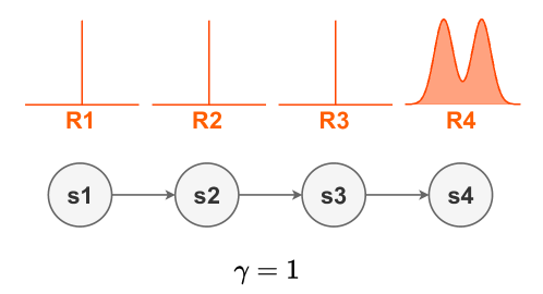
Figure 4: Toy Markov decision process

References

- Ball et al. [2023] Philip J. Ball, Laura Smith, Ilya Kostrikov, and Sergey Levine. Efficient online reinforcement learning with offline data. arXiv preprint arXiv:2302.02948, 2023.
- Bellemare et al. [2017] Marc G. Bellemare, Will Dabney, and Rémi Munos. A distributional perspective on reinforcement learning. In ICML, pages 449–458. PMLR, 2017.
- Bellemare et al. [2023] Marc G. Bellemare, Will Dabney, and Mark Rowland. Distributional Reinforcement Learning. MIT Press, 2023.
- Cavazos et al. [2020] Jacqueline G Cavazos, P Jonathon Phillips, Carlos D Castillo, and Alice J O’Toole. Accuracy comparison across face recognition algorithms: Where are we on measuring race bias? IEEE Transactions on Biometrics, Behavior, and Identity Science, 3(1):101–111, 2020.
- Chen et al. [2021] Xinyue Chen, Che Wang, Zijian Zhou, and Keith W. Ross. Randomized ensembled double q-learning: Learning fast without a model. In ICLR, 2021.
- Chow et al. [2017] Yinlam Chow, Mohammad Ghavamzadeh, Lucas Janson, and Marco Pavone. Risk-constrained reinforcement learning with percentile risk criteria. JMLR, 18(1):6070–6120, 2017.
- Dabney et al. [2018a] Will Dabney, Georg Ostrovski, David Silver, and Rémi Munos. Implicit quantile networks for distributional reinforcement learning. In ICML, pages 1096–1105. PMLR, 2018a.
- Dabney et al. [2018b] Will Dabney, Mark Rowland, Marc Bellemare, and Rémi Munos. Distributional reinforcement learning with quantile regression. In Proceedings of the AAAI Conference on Artificial Intelligence, volume 32, 2018b.
- Duan et al. [2022] Jingliang Duan, Yang Guan, Shengbo Eben Li, Yangang Ren, Qi Sun, and Bo Cheng. Distributional soft actor-critic: Off-policy reinforcement learning for addressing value estimation errors. IEEE Transactions on Neural Networks and Learning Systems, 33(11):6584–6598, 2022.
- Fan et al. [2023] Zimeng Fan, Nianli Peng, Muhang Tian, and Brandon Fain. Welfare and fairness in multi-objective reinforcement learning. In AAMAS, 2023.
- foundation [2023] Farama foundation. Gymnasium, 2023. URL https://github.com/Farama-Foundation/Gymnasium.
- Haarnoja et al. [2018] Tuomas Haarnoja, Aurick Zhou, Pieter Abbeel, and Sergey Levine. Soft actor-critic: Off-policy maximum entropy deep reinforcement learning with a stochastic actor. arXiv preprint arXiv:1801.01290, 2018.
- He [1997] Xuming He. Quantile curves without crossing. The American Statistician, 51(2):186–192, 1997.
- Hiraoka et al. [2022] Takuya Hiraoka, Takahisa Imagawa, Taisei Hashimoto, Takashi Onishi, and Yoshimasa Tsuruoka. Dropout q-functions for doubly efficient reinforcement learning. In ICLR, 2022.
- Hoerl [1962] Arthur E. Hoerl. Application of ridge analysis to regression problems. Chemical Engineering Progress, 58:54–59, 1962.
- Huang et al. [2022] Shengyi Huang, Rousslan Fernand Julien Dossa, Chang Ye, Jeff Braga, Dipam Chakraborty, Kinal Mehta, and João G.M. Araújo. Cleanrl: High-quality single-file implementations of deep reinforcement learning algorithms. JMLR, 23(274):1–18, 2022.
- Jullien et al. [2023] Sami Jullien, Mozhdeh Ariannezhad, Paul Groth, and Maarten de Rijke. A simulation environment and reinforcement learning method for waste reduction. TMLR, 2023.
- Kostas et al. [2021] James Kostas, Yash Chandak, Scott M Jordan, Georgios Theocharous, and Philip Thomas. High confidence generalization for reinforcement learning. In ICML, pages 5764–5773. PMLR, 2021.
- Kostrikov et al. [2022] Ilya Kostrikov, Ashvin Nair, and Sergey Levine. Offline reinforcement learning with implicit q-learning. In ICLR, 2022.
- Ma et al. [2021] Yecheng Ma, Dinesh Jayaraman, and Osbert Bastani. Conservative offline distributional reinforcement learning. In NeurIPS, volume 34, pages 19235–19247. Curran Associates, Inc., 2021.
- Martin et al. [2020] John Martin, Michal Lyskawinski, Xiaohu Li, and Brendan Englot. Stochastically dominant distributional reinforcement learning. In ICML, volume 119, pages 6745–6754. PMLR, 13–18 Jul 2020.
- Mavrin et al. [2019] Borislav Mavrin, Hengshuai Yao, Linglong Kong, Kaiwen Wu, and Yaoliang Yu. Distributional reinforcement learning for efficient exploration. In ICML, pages 4424–4434. PMLR, 2019.
- Metelli et al. [2023] Alberto Maria Metelli, Mirco Mutti, and Marcello Restelli. A tale of sampling and estimation in discounted reinforcement learning. In Proceedings of The 26th International Conference on Artificial Intelligence and Statistics, volume 206, pages 4575–4601. PMLR, 25–27 Apr 2023.
- Mnih et al. [2013] Volodymyr Mnih, Koray Kavukcuoglu, David Silver, Alex Graves, Ioannis Antonoglou, Daan Wierstra, and Martin Riedmiller. Playing Atari with deep reinforcement learning. arXiv preprint arXiv:1312.5602, 2013.
- Newey and Powell [1987] Whitney K. Newey and James L. Powell. Asymmetric least squares estimation and testing. Econometrica, 55(4):819–847, 1987.
- Paszke et al. [2019] Adam Paszke, Sam Gross, Francisco Massa, Adam Lerer, James Bradbury, Gregory Chanan, Trevor Killeen, Zeming Lin, Natalia Gimelshein, Luca Antiga, Alban Desmaison, Andreas Kopf, Edward Yang, Zachary DeVito, Martin Raison, Alykhan Tejani, Sasank Chilamkurthy, Benoit Steiner, Lu Fang, Junjie Bai, and Soumith Chintala. Pytorch: An imperative style, high-performance deep learning library. In NeurIPS, pages 8024–8035. Curran Associates, Inc., 2019.
- Philipps [2021a] Colin Philipps. When is an expectile the best linear unbiased estimator? SSRN, 2021a.
- Philipps [2021b] Collin Philipps. Interpreting expectiles. SSRN, 2021b.
- Polyak and Juditsky [1992] Boris T. Polyak and Anatoli B. Juditsky. Acceleration of stochastic approximation by averaging. SIAM Journal on Control and Optimization, 30(4):838–855, 1992.
- Rowland et al. [2019] Mark Rowland, Robert Dadashi, Saurabh Kumar, Rémi Munos, Marc G. Bellemare, and Will Dabney. Statistics and samples in distributional reinforcement learning. In ICML, pages 5528–5536. PMLR, 2019.
- Rowland et al. [2023] Mark Rowland, Rémi Munos, Mohammad Gheshlaghi Azar, Yunhao Tang, Georg Ostrovski, Anna Harutyunyan, Karl Tuyls, Marc G. Bellemare, and Will Dabney. An analysis of quantile temporal-difference learning. arXiv preprint arXiv:2301.04462, 2023.
- Strens [2000] Malcolm Strens. A Bayesian framework for reinforcement learning. In ICML, volume 2000, pages 943–950, 2000.
- Sutton and Barto [2018] Richard S. Sutton and Andrew G. Barto. Reinforcement Learning: An Introduction. MIT press, 2018.
- Todorov et al. [2012] Emanuel Todorov, Tom Erez, and Yuval Tassa. Mujoco: A physics engine for model-based control. In 2012 IEEE/RSJ International Conference on Intelligent Robots and Systems, pages 5026–5033. IEEE, 2012.
- Vlassis et al. [2012] Nikos Vlassis, Mohammad Ghavamzadeh, Shie Mannor, and Pascal Poupart. Bayesian reinforcement learning. Reinforcement Learning: State-of-the-Art, pages 359–386, 2012.
- Waltrup et al. [2015] Linda Schulze Waltrup, Fabian Sobotka, Thomas Kneib, and Göran Kauermann. Expectile and quantile regression—david and goliath? Statistical Modelling, 15(5):433–456, 2015.
- Yang et al. [2019] Derek Yang, Li Zhao, Zichuan Lin, Tao Qin, Jiang Bian, and Tie-Yan Liu. Fully parameterized quantile function for distributional reinforcement learning. NeurIPS, 32, 2019.
- Yao and Tong [1996] Qiwli Yao and Howell Tong. Asymmetric least squares regression estimation: A nonparametric approach. Journal of Nonparametric Statistics, 6(2-3):273–292, 1996.
- Zhang and Yao [2019] Shangtong Zhang and Hengshuai Yao. Quota: The quantile option architecture for reinforcement learning. In AAAI. AAAI Press, 2019.