Modelling, Analysis, and Control of OmniMorph: an Omnidirectional Morphing Multi-rotor UAV

Abstract

This paper introduces for the first time the design, modelling, and control of a novel morphing multi-rotor Unmanned Aerial Vehicle (UAV) that we call the OmniMorph. The morphing ability allows the selection of the configuration that optimizes energy consumption while ensuring the needed maneuverability for the required task. The most energy-efficient uni-directional thrust (UDT) configuration can be used, e.g., during standard point-to-point displacements. Fully-actuated (FA) and omnidirectional (OD) configurations can be instead used for full pose tracking, such as, e.g., constant attitude horizontal motions and full rotations on the spot, and for full wrench 6D interaction control and 6D disturbance rejection. Morphing is obtained using a single servomotor, allowing possible minimization of weight, costs, and maintenance complexity. The actuation properties are studied, and an optimal controller that compromises between performance and control effort is proposed and validated in realistic simulations.

1 Introduction

Over the last decade, the design, perception, and control of Unmanned Aerial Vehicles (UAVs) have substantially evolved in terms of functionalities and capabilities indoors or outdoors. Research now considers the use of UAVs as Aerial Robotic Manipulators that can interact physically with the environment [1] and humans [2]; contact-based inspection [3], object manipulation [4], and assisting human workers [5] are some of the typical tasks.

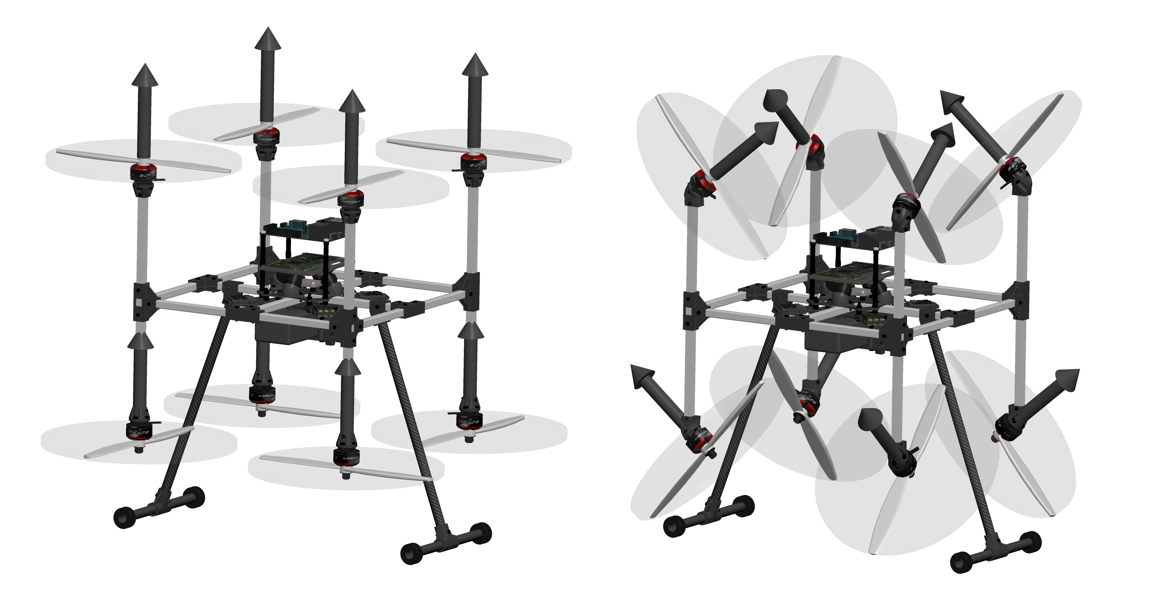
Figure 1: OmniMorph: UA configuration (left) and OD configuration (right).

This led to the development of new multi-rotor aerial vehicles (MRAVs) and especially to the exploration of designs different from the popular underactuated multirotors that use fixed coplanar/collinear propellers (i.e., quadrotors, hexarotors, and their variants). The new designs rely on choosing the number, position, and orientation of the propellers to provide the multirotor with different actuation properties and abilities to achieve a specific task [6].

Recently, several works addressed the design of omnidirectional multirotors. Omnidirectionality is the property of the robot to sustain its weight in any orientation. In the literature, different actuation strategies to achieve omnidirectionality have been proposed. In [7], a novel metric to assess the omnidirectional property of a generic multi-rotor aerial vehicle was presented. This metric is calculated numerically from the force set of the platform, and as such it relies on the platform geometry and thrusters; moreover, it allows a direct assessment of a platform’s omnidirectional property given its weight. [7] also showed the use of this metric in the process of upgrading the design presented in [8], by placing the propellers on a virtual sphere centered around the platform’s center of masss (CoMs) instead of the same plane with the platform’s CoM. In the following, we categorize omnidirectional designs into three main classes.

The first class uses fixedly tilted bi-directional propellers (which generate thrust in both directions by inverting their sense of rotation). The authors in [9] presented one of the first omnidirectional prototypes, where they placed eight bi-directional propellers on the edges of a cube. The novelty of their design is the optimization-based placement and orientation of the propellers, where the cube shape was chosen to ensure a rotation-invariant inertia tensor. Another omnidirectional design with fixed propellers was presented in [10] and [11], achieving omnidirectional wrench generation with six and eight bi-directional propellers, respectively.

The second class, like the design proposed in [12], optimizes the orientation of fixed uni-directional propellers (i.e., able to produce thrust in only one direction, or, in other words, to rotate in only one sense) to achieve omnidirectionality while equally distributing the thrust produced by each propeller and aiming for an isotropic (sphere-like) shape of the corresponding force set. In fact, [12] showed that the minimal number of 7 (seven) uni-directional propellers is necessary to achieve omnidirectional position and orientation tracking. Later, [8] presented a working prototype of the design with experiments.

The third class of omnidirectional platforms relies on a morphing design. Uni- or bi-directional propellers actively tilted by servo motors are used. [13] proposes a quadrotor with propellers individually tilting about their radial axis. The authors of [14] use the same idea (independently controlled radially tilting thrusters) for an hexarotor. Another version of their design was presented in [15], in which double propeller groups were used, two propellers rotating in opposite directions on each rotation axis to increase the platform efficiency and payload capacity in addition to increased force bounds along different directions.

The advantage of the third design approach relies on the possibility to optimize the energy consumed for a given desired orientation, which is obtained by aligning together as much as possible the propeller spinning directions for a given orientation, in a way that each propeller tends to be as much counter aligned as possible to the gravity force. This also allows for balancing dexterity and energy efficiency based on the needs imposed by specific tasks [16] [17]. Indeed, the configuration in which all the directions are aligned is more energetically efficient. In that configuration, the propeller forces are all parallel to each other but the thrust is uni-directional; when this is not the case, there are propeller forces that cancel each other without actively contributing to the motion. That is the price paid to achieve multi/omnidirectionality.

From a control allocation point of view, fixed-propeller multirotors in [9], [10], [8] are controlled by (pseudo)inverting the wrench map between the propellers’ speeds and the total body wrench. Those systems are affine in the control inputs and the tilting angles of the propellers are constant design parameters. A similar control approach is used in [11], where a different rotor input allocation is proposed, based on the infinity-norm minimization; in this way, propellers’ speed constraints are implicitly taken into account, even though with no guarantees. For the second type of omnidirectional platforms, in [8] a dynamic inversion plus input allocation strategy is proposed. The input allocation modifies the minimum norm solution found by inverting the allocation matrix to ensure that the rotational speeds are positive.

The control of the third class of platforms is challenging, as the tilting angle must also be determined, which appears nonlinearly in the dynamics. Feedback linearization at the jerk level has been proposed [13], thanks to the fact that the time-differentiation the system is affine in the (new) control inputs. In [14], a change of variables is used to obtain a static allocation matrix not dependent on the tilting angle; that is pseudo-inverted, and the initial inputs are then computed. Both these methods require the full allocation matrix to be non-singular and may result in unfeasible inputs due to neglected input bounds. [15] proposes a jerk-level control in which the optimal control inputs are obtained by weighted pseudo-inversion of the full allocation matrix. As input constraints are not considered, the inputs are saturated before being integrated and sent to the actuators. The control method avoids singularities by adding a bias to the desired tilting angle in case of a large condition number of the wrench map matrix.

In this work, we overcome some of the limitations of existing concepts and controllers of omnidirectional platforms. Specifically, the contributions of this work are as follows.

• A novel omnidirectional morphing platform design concept, OmniMorph, is proposed. The platform belongs to the third class described in this section and exploits the synchronized drive of all propellers by only one servo motor. This choice allows keeping at the bare minimum the additional payload used to carry additional servo motors in the other designs seen before.

• The actuation properties of OmniMorph are formally studied.

• A novel control method is proposed for multi-rotors with actively and synchronously tilting propellers. Compared to the state of the art, the proposed controller allows automatic transitions between underactuated and omnidirectional configurations while explicitly accounting for input constraints, only indirectly handled through redundancy resolution in the literature [13].

• The proposed design and controller are tested in a realistic simulation environment.

2 OmniMorph Design and model

2.1 Concept and Design

The OmniMorph platform consists of 8 bi-directional propellers attached to the main body frame, placed on the vertices of a cube centered at the CoM, as in Figure 1. The idea of this work is to design a morphing platform, i.e., capable of tilting its propellers, that can span, while flying, a variety of configurations in between two extreme cases: a dexterous but less energetically efficient omnidirectional configuration and an efficient but underactuated unilateral thrust configuration. More than that, we ask that all propellers tilt in a synchronized way, meaning they can be all attached to a single extra actuation unit (a tilting mechanism) driven by only one servo motor. That reduces the complexity and the weight of the prototype, allowing for a higher payload.

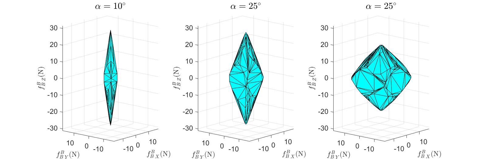
Figure 2: Sets of feasible forces for different values of $\alpha$. The three components of the thrust in the body frame are displayed. OmniMorph is omnidirectional when a sphere with a radius equal to the robot’s weight is inscribed inside the polytope of feasible forces.

Note that each propeller tilts about a different axis of the same amount, which we call the tilting angle $\alpha.$ The change in the orientation of the propellers (morphing), changes (i.e., it morphs) the force and moment feasible sets. When all rotors are parallel to each other (i.e. titling angle $\alpha$ equal to zero) the force set is a thin line, i.e., the generated total thrust can be produced only along one axis, making the vehicle underactuated (UA)—see Figure 1 left. In this case, the platform is, from the actuation point of view, equivalent to the standard underactuated quadrotor, hexarotor, and so on: only 4 DoF s are independently controlled, the 3D position and the heading angle. This configuration is the most energetically efficient and it is recommended in tasks in which the control of the full orientation or full wrench is not essential.

When the tilting angle $\alpha$ assumes positive values, the feasible force set morphs into a polyhedron with non-zero volume. The larger the tilting angle the larger the volume. The total thrust can be generated in all three orthogonal directions, to a certain extent, depending on the tilting angle value. Ultimately, the vehicle can assume an OD configuration similar to the vehicle developed in [9]—see Figure 1, right. Such a configuration allows controlling the 6D full pose of the vehicle sustaining its weight in any possible orientation. A representation of the polytopes of feasible forces of OmniMorph for different values of $\alpha$ computed as in [6] is given in Figure 2.

In the following, the design concept of OmniMorph is detailed. We define a reference frame attached to the robot as a set of an origin and three orthogonal axes: ${\mathcal{F}_{B}:\{O_{B},\mathbf{x}_{B},\mathbf{y}_{B},\mathbf{z}_{B}\}}$, where the origin, $O_{B}$, is coincident with the robot CoM. Hence, as in [18], the matrix whose columns are the positions of each propeller’s center $O_{p_{i}}$ in the body frame, call it $\mathbf{P}=[\bm{p}_{p_{1}}^{B},...,\bm{p}_{p_{8}}^{B}]$, is given by:

$$\mathbf{P}=\frac{L}{\sqrt{3}}\begin{bmatrix}1&-1&1&-1&1&-1&1&-1\\ 1&1&-1&-1&1&1&-1&-1\\ 1&1&1&1&-1&-1&-1&-1\end{bmatrix},$$ (1)

where the propellers are numbered as in Figure 3 and $L$ is a geometric parameter equal to half the length of the cube edge connecting the propellers.

The work in [18] computes some fixed orientations of each propeller to attain omnidirectionality. Especially, in that work, the coordinates in $\mathcal{F}_{B}$ of the thrust unit vectors for the fixed tilted propellers, call them $\bm{b}_{p_{i}}$, are collected in the matrix $\mathbf{B}=[\bm{b}_{p_{1}}\cdots\bm{b}_{p_{8}}]$ given by

$$\mathbf{B}=\begin{bmatrix}-a&b&-b&a&a&-b&b&-a\\ b&a&-a&-b&-b&-a&a&b\\ c&-c&-c&c&c&-c&-c&c\end{bmatrix},$$ (2)

where $a=\frac{1}{2}+\frac{1}{\sqrt{12}},$ $b=\frac{1}{2}-\frac{1}{\sqrt{12}},$ and $c=\frac{1}{\sqrt{3}}$.

Define now as $\bm{b^{\prime}}_{p_{i}}$ the coordinates of the unit vector, centered on $O_{p_{i}}$, that describes the axis of rotation of propeller $i-$th that brings it from the attitude described by (2) to a configuration in which its thrust direction is parallel to $\mathbf{z}_{B},$ thus bringing the robot into the unilateral-thrust configuration. We have that $\bm{b^{\prime}}_{p_{i}}$ is given by the cross product between $\bm{b}_{p_{i}}$ and $\bm{e}_{3}$, where $\bm{e}_{i}$ is the $i-$th column of the identity matrix $\mathbf{I}_{3}\in\mathbb{R}^{3\times 3}.$

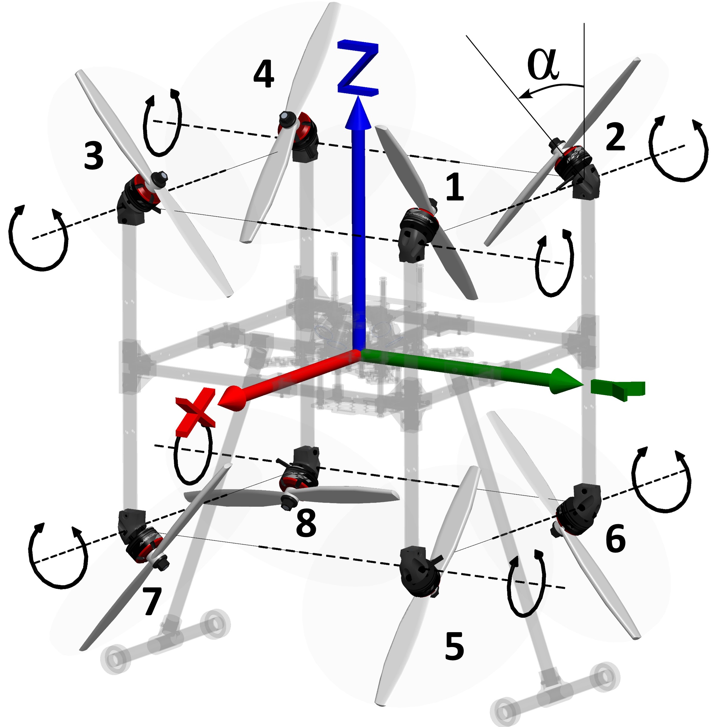
Figure 3: Representation of OmniMorph in which the axes of rotation of the propellers, lying along the cube edges, are highlighted.

Very interestingly, $\bm{b^{\prime}}_{p_{i}}$ is orthogonal to $\bm{b^{\prime}}_{p_{j}}$ $\forall i\in\{1,4,5,8\}$, $\forall j\in\{2,3,6,7\}.$ More than that, by rotating of $\frac{\pi}{12}$ radians (i.e., $15\,\rm{deg}$) around $\mathbf{z}_{B}$ the cube whose edges lie along these axes, one obtains the cube formed connecting the propeller positions. Such a symmetric configuration greatly simplifies the mechanical realization of the tilting mechanism, and, as it will be more clear in the following, is still omnidirectional. Hence, the propeller tilting axes of OmniMorph are conveniently chosen along the edges of the cube whose vertices host the propellers centers—see Figure 3.

To summarize formally, the positions of the centers of the propellers are given in (1), and the attitude is described as follows. Define a frame attached to each propeller ${\mathcal{F^{\prime}}_{p_{i}}:\{O_{p_{i}},\mathbf{x^{\prime}}_{i},\mathbf{y^{\prime}}_{i},\mathbf{z^{\prime}}_{i}\}}$, where $\mathbf{x^{\prime}}_{i}=\bm{b^{\prime}}_{p_{i}}$, $\mathbf{z^{\prime}}_{i}=\mathbf{z}_{B},$ and $\mathbf{y^{\prime}}_{i}$ is chosen orthogonal to the first two. Denote the rotation matrix between ${\mathcal{F}_{B}}$ and ${\mathcal{F^{\prime}}_{p_{i}}}$ with $\mathbf{R^{\prime}}_{p_{i}}$. Eventually, the rotation between ${\mathcal{F}_{B}}$ and each propeller’s frame ${\mathcal{F}_{p_{i}}:\{O_{p_{i}},\mathbf{x}_{i},\mathbf{y}_{i},\mathbf{z}_{i}\}}$ is given by ${{}^{B}\mathbf{R}_{p_{i}}(\alpha)=\mathbf{R^{\prime}}_{p_{i}}\mathbf{R}_{Z}\left(\frac{\pi}{12}\right)\mathbf{R}_{X}(\alpha),}$ where $\mathbf{R}_{X}()$ $\mathbf{R}_{Z}()$ are the elementary rotations about the $X$ and $Z$ axes. Each propeller exerts its thrust along the axis $\mathbf{z}_{i}$ which is rotated by $\alpha$ about an axis lying along the edges of the cube that connects the propellers’ centers.

$\alpha=0$	$\alpha=\frac{\pi}{2}$	$\alpha\neq\frac{\pi}{2},\pi,0$
Underactuated	Fully Actuated unless $\bm{u}_{\omega}=0$	Fully Actuated, Redundant

Table 1: Actuation properties for different values of $\alpha$. Grey circles are the propellers’ planes. Each is associated with a local frame, and a body-fixed frame is in the middle of the robot. The RGB convention is used to indicate the x-, y-, and z- axis, respectively. The direction of the thrust produced by the individual propellers is represented with a thick black arrow.

2.2 Model of the OmniMorph

In this section, the dynamics equations of OmniMoprh are given. Let us define an inertial frame $\mathcal{F}_{W}:\{O_{W},\mathbf{x}_{W},\mathbf{y}_{W},\mathbf{z}_{W}\}$. The position of $O_{B}$ in $\mathcal{F}_{W}$ is indicated as $\bm{p}$ and its attitude is expressed compactly as $\mathbf{R}:=^{W}\mathbf{R}_{B}$.

The dynamic equations of the robot, expressed as Newton-Euler equations of an actuated rigid body, are as follows, where the translational dynamics is expressed in the inertial frame and the rotational dynamics in the body frame. We indicate as $\boldsymbol{\omega}$ the angular velocity of $\mathcal{F}_{B}$ w.r.t. $\mathcal{F}_{W}$ expressed in $\mathcal{F}_{B}$, with $m$ the robot mass, and with $\mathbf{J}\in\mathbb{R}^{3\times 3}$ its rotational inertia.

$$\begin{bmatrix}m\mathbf{I}_{3}&\boldsymbol{0}_{3}\\ \boldsymbol{0}_{3}&\mathbf{J}\end{bmatrix}\begin{bmatrix}\ddot{\bm{p}}\\ \dot{\boldsymbol{\omega}}\end{bmatrix}=\begin{bmatrix}-mg\bm{e}_{3}\\ -\boldsymbol{\omega}\times\mathbf{J}\boldsymbol{\omega}\end{bmatrix}+\begin{bmatrix}\mathbf{R}&\boldsymbol{0}_{3}\\ \boldsymbol{0}_{3}&\mathbf{I}_{3}\end{bmatrix}\begin{bmatrix}\bm{f}_{B}^{B}\\ \boldsymbol{\tau}_{B}^{B}\end{bmatrix}$$ (3)

$\bm{f}_{B}^{B}$ and $\boldsymbol{\tau}_{B}^{B}$ are the total force and torque applied to the CoM, expressed in ${\mathcal{F}_{B}}$.

The rotational kinematics of the robot is:

$$\dot{\mathbf{R}}=\mathbf{R}[\boldsymbol{\omega}]_{\times}.$$ (4)

where $[\boldsymbol{\omega}]_{\times}$ is the skew symmetric matrix associated to $\boldsymbol{\omega}$. Each rotor produces a thrust force and a drag moment which we model, similarly to [19], as follows.

$$\bm{f}_{i}=c_{f}w_{i}|w_{i}|\mathbf{z}_{i},\quad\bm{\tau}_{d_{i}}=-k_{i}c_{\tau}w_{i}|w_{i}|\mathbf{z}_{i},$$ (5)

where $c_{f},c_{\tau}>0$ are the thrust and drag coefficient, respectively, and $w_{i}$ is a scalar with a module equal to the norm of the propeller angular velocity and a sign defined such that $w_{i}>0$ when the thrust produced by the propeller has the same direction of $\mathbf{z}_{i}$. The drag moment is always opposite to the angular velocity of the propeller; as a consequence, $k_{i}=-1$ for propellers with descending chord (i.e., producing thrust in the same direction of the angular velocity, also called ‘counterclockwise’) and $k_{i}=+1$ for propellers with ascending chord (i.e., producing thrust in the opposite direction of the angular velocity, also called ‘clockwise’). The applied body forces and torques are the results of all propellers and their orientation:

$$\bm{f}_{B}^{B}=\sum_{i=1}^{n}\bm{f}_{i}^{B}=\sum_{i=1}^{n}\prescript{B}{}{\mathbf{R}_{p_{i}}}\bm{e}_{3}f_{i}$$ (6)

$$\begin{split}\boldsymbol{\tau}_{B}^{B}&=\sum_{i=1}^{n}\boldsymbol{\tau}_{f_{i}}^{B}+\boldsymbol{\tau}_{d_{i}}^{B}=\sum_{i=1}^{n}\bm{p}_{p_{i}}^{B}\times\bm{f}_{i}^{B}-k_{i}c_{f}^{\tau}\bm{f}_{i}^{B}\\ &=\sum_{i=1}^{n}([\bm{p}_{p_{i}}^{B}]_{\times}-k_{i}c_{f}^{\tau}\mathbf{I}_{3})\prescript{B}{}{\mathbf{R}_{p_{i}}}\bm{e}_{3}f_{i}\end{split}$$ (7)

where $c_{f}^{\tau}=c_{\tau}/c_{f}$. We indicated with $\bm{f}_{i}^{B}$ the thrust force of the $i$-th propeller expressed in $\mathcal{F}_{B}$, and with $\boldsymbol{\tau}_{f_{i}}^{B}$ and $\boldsymbol{\tau}_{d_{i}}^{B}$ the torque produced by the same propeller’s thrust at the CoM and the effect of the propeller’s drag torque at the CoM, respectively.

We denote with $\boldsymbol{u}$ the input of the system, consisting of the single morphing angle ${\alpha}$ and the rotor speeds contained in the vector $\boldsymbol{u}_{w}$ such that

$$\boldsymbol{u}_{w}=[u_{w_{1}}\cdots u_{w_{n}}]^{\top}=[w_{1}|w_{1}|\cdots w_{n}|w_{n}|]^{\top}\in\mathbb{R}^{n}.$$ (8)

Hence, one has $\boldsymbol{u}=\begin{bmatrix}\boldsymbol{u}_{w}^{\top}&\alpha\end{bmatrix}^{\top}\in\mathbb{R}^{9}.$ Based on (6) and (7), we have that the actuation wrench is

$$\mathbf{w}(\boldsymbol{u})=\begin{bmatrix}\bm{f}_{B}^{B}\\ \boldsymbol{\tau}_{B}^{B}\end{bmatrix}=\mathbf{A}(\alpha)\boldsymbol{u}_{\omega}.$$ (9)

Please note that the full expression of $\mathbf{A}(\alpha)$ is given at the end of Sec. 2.3.

2.3 Actuation Properties

First, we define the full allocation matrix ${\mathbf{F}(\boldsymbol{u})\in\mathbb{R}^{6\times 9}}$ as in [6]:

$$\mathbf{F}(\boldsymbol{u})=\begin{bmatrix}\mathbf{F}_{1}(\alpha)&\mathbf{F}_{2}(\boldsymbol{u}_{\omega},\alpha)\end{bmatrix}$$ (10)

with $\mathbf{F}_{1}(\alpha)=\frac{\partial\mathbf{w}}{\partial\boldsymbol{u}_{w}}(\alpha)\in\mathbb{R}^{6\times 8},\mathbf{F}_{2}(\boldsymbol{u})=\frac{\partial\mathbf{w}}{\partial{\alpha}}(\boldsymbol{u})\in\mathbb{R}^{6}.$ Note that, for (9), $\mathbf{F}_{1}=\mathbf{A}(\alpha)$ and $\mathbf{F}_{2}=\frac{\partial(\mathbf{A}(\alpha)\boldsymbol{u}_{w})}{\partial\alpha}.$ Following the method provided in [6], we study the actuation properties of the platform by looking at the rank of $\mathbf{F}(\boldsymbol{u})$ in (10). For all the points in the input space in which $\text{rank}(\mathbf{F}(\boldsymbol{u}))=6$ (full rank), the platform is fully actuated. In those points, the actuation wrench can be changed in every direction by suitably acting on the input. Instead, in all points in which $\text{rank}(\mathbf{F}(\boldsymbol{u}))<6$ (rank deficient) the platform is underactuated, this means that when the input is in those singular points there are some forbidden directions along which the actuation wrench cannot be changed.

First, we note that studying the rank of t$\mathbf{F}(\boldsymbol{u})$ is $6\times 9$ helps us study the rank of the full allocation matrix, $\mathbf{F}(\boldsymbol{u})$:

• $\rm{rank}(\mathbf{F}_{1}(\alpha))=4$ is a sufficient condition for the platform to be underactuated: the rank of the full allocation matrix $\mathbf{F}(\bm{u})$ can be at most $5<6$.

• $\rm{rank}(\mathbf{F}_{1}(\alpha))=6$ is a sufficient condition for the system to be fully actuated;

• If $\rm{rank}(\mathbf{F}_{1}(\alpha))=5$, the full-/under-actuation needs further analysis of $\mathbf{F}_{2}(\boldsymbol{u})\in\mathbb{R}^{6\times 1}$ in relation to $\mathbf{F}_{1}(\alpha)$.

Hence, we study the rank of $\mathbf{F}_{1}(\alpha)$ for various values of $\alpha$, finding that

$$\rm{rank}(\mathbf{F}_{1}(\boldsymbol{\alpha}))=\begin{cases}4&\rm{if}\ \alpha=0+k\pi,k\in\mathbb{N}\\ 5&\rm{if}\ {\alpha}=\frac{\pi}{2}\\ 6&\ \rm{otherwise}\\ \end{cases}$$ (11)

So, from what has been said so far, OmniMorph is underactuated for $\alpha=0$. Moreover, ${\rm{rank}}({\mathbf{F}}{(\bm{u}_{w},0))}=5$ if $\boldsymbol{u}_{w}\neq\bm{0}$ and if not all ${u_{w}}_{i}$ are equal to each other, i.e., the total wrench can be instantaneously changed on a ‘reduced’ five-dimensional manifold.

For $\alpha=\pi/2$, OmniMorph is in general under-actuated. However, it is fully actuated ($\rm{rank}(\mathbf{F}(\boldsymbol{u}_{w},\pi/2))=6)$ if $\boldsymbol{u}_{w}\neq\bm{0}$. An intuitive interpretation is provided in the following. When $\alpha=\pi/2,$ all propellers’ thrusts are on the same plane in $\mathcal{F}_{B}$.

The yaw acceleration can be changed as the individual thrusts generate a torque around the vertical axis of the robot. The pitch and roll accelerations can be changed thanks to the drag moment of the propellers. The translational acceleration in the horizontal plane is clearly changeable by the thrust, but the translational acceleration along $\mathbf{z}_{B}$ is not. As soon as $\alpha$ changes, the propellers’ thrusts have a component in the vertical direction as well, which gives control of the vertical acceleration, unless the propellers’ thrusts are actually zero (mathematically, $\boldsymbol{u}_{w}=\bm{0}$).

Please note that even if the platform is fully actuated it might not be able to fly properly because the propeller thrust intensity may be not large enough to sustain the platform’s weight.

Eventually, for all other values of $\alpha$, the platform is fully actuated. A schematic summary of the OmniMorph actuation properties is in Table 1.

For sufficiently large values of $\alpha,$ the polygon of the achievable forces, see Fig. 2 contains a sphere whose radius corresponds to the weight of the platform: the robot can sustain its weight in any orientation; thus, it is omnidirectional.

The full allocation matrix is reported in the following for the sake of completeness:

$$\mathbb{F}=\frac{1}{c_{f}}\left[\scalebox{0.9}[1.0]{$\begin{matrix}-s_{\alpha}&0&s_{\alpha}\\ 0&s_{\alpha}&-s_{\alpha}&0\\ c_{\alpha}&c_{\alpha}&c_{\alpha}&c_{\alpha}\\ Lc_{\alpha}-\frac{c_{\tau}s_{\alpha}}{c_{f}}&Lc_{\alpha}+Ls_{\alpha}&\frac{c_{\tau}s_{\alpha}}{c_{f}}-Lc_{\alpha}&-Lc_{\alpha}-Ls_{\alpha}\\ -Lc_{\alpha}-Ls_{\alpha}&Lc_{\alpha}+\frac{c_{\tau}s_{\alpha}}{c_{f}}&Lc_{\alpha}+Ls_{\alpha}&-Lc_{\alpha}-\frac{c_{\tau}s_{\alpha}}{c_{f}}\\ Ls_{\alpha}+\frac{c_{\tau}c_{\alpha}}{c_{f}}&Ls_{\alpha}-\frac{c_{\tau}c_{\alpha}}{c_{f}}&Ls_{\alpha}+\frac{c_{\tau}c_{\alpha}}{c_{f}}&Ls_{\alpha}-\frac{c_{\tau}c_{\alpha}}{c_{f}}\\ \end{matrix}$}\right.$$

$$\left.\scalebox{0.85}[1.0]{$\begin{matrix}s_{\alpha}&0&0&-s_{\alpha}\\ 0&-s_{\alpha}&s_{\alpha}&0&\\ c_{\alpha}&c_{\alpha}&c_{\alpha}&c_{\alpha}\\ Lc_{\alpha}+\frac{c_{\tau}s_{\alpha}}{c_{f}}&-Lc_{\alpha}-Ls_{\alpha}&-Lc_{\alpha}+Ls_{\alpha}&-Lc_{\alpha}-\frac{c_{\tau}s_{\alpha}}{c_{f}}\\ -Lc_{\alpha}-Ls_{\alpha}&\frac{c_{\tau}s_{\alpha}}{c_{f}}-Lc_{\alpha}&Lc_{\alpha}-\frac{c_{\tau}s_{\alpha}}{c_{f}}&Lc_{\alpha}+Ls_{\alpha}\\ \frac{c_{\tau}c_{\alpha}}{c_{f}}-Ls_{\alpha}&-Ls_{\alpha}-\frac{c_{\tau}c_{\alpha}}{c_{f}}&-Ls_{\alpha}-\frac{c_{\tau}c_{\alpha}}{c_{f}}&\frac{c_{\tau}c_{\alpha}}{c_{f}}-Ls_{\alpha}\end{matrix}$}\small{\frac{\partial\mathbf{w}}{\partial\alpha}}\right]$$

2.4 Power Consumption Analysis

To analyze the power consumption of the OmniMorph in comparison with a non-morphing fully actuated platform, let us start by computing the input needed to enforce the static equilibrium when the platform is hovering with orientation $\mathbf{R}=\mathbf{I}_{3}$, this can be done by inverting (9) as

$$\boldsymbol{u}^{h}_{w}(\alpha,m)=\left(\mathbf{A}(\alpha)\right)^{\dagger}\begin{bmatrix}mg\bm{e}_{3}\\ \bm{0}\end{bmatrix}.$$ (12)

The power consumed by each brushless motor is equal to the scalar product between the motor torque and its angular velocity. Given that in hovering we can approximate the motor torque with the drag moment and that the drag moment is always opposing the angular velocity, we can write the power consumed by the $i$-th brushless motor as $P(u_{w_{i}})=\|\boldsymbol{\tau}_{d_{i}}\||w_{i}|=c_{\tau}|w_{i}|^{3}=c_{\tau}|u_{w_{i}}|^{3/2}$. The total power consumed by all the motors is then

$$P_{\text{tot}}(\boldsymbol{u}_{w})=\sum_{i=1}^{8}P(u_{w_{i}})=c_{\tau}\sum_{i=1}^{8}|u_{w_{i}}|^{3/2}.$$ (13)

Therefore, $P_{\text{tot}}(\boldsymbol{u}^{h}_{w}(\alpha,m))$ represents the power consumed at hovering by a platform with a certain mass $m$ and a given tilting angle $\alpha$.

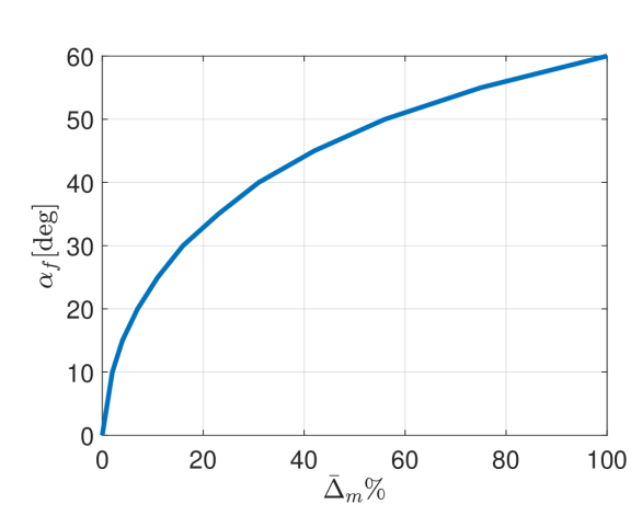
Figure 4: For a given fixed propeller tilting angle $\alpha_{f}$, a morphing design is convenient, provided that the relative mass of the tilting mechanism is lower than $\bar{\Delta}_{m}$

Let us now write the robot’s mass as follows: $m=m_{0}(1+\Delta_{m})$, where $\Delta_{m}$ is the ratio between the mass of the propeller tilting mechanism and $m_{0}$, which is the mass of all other components. Consider a multirotor in which a certain level of dexterity is obtained by tilting the propellers by a fixed angle $\alpha_{f}$. We ask ourselves which is the critical relative mass of a tilting mechanism, $\bar{\Delta}_{m},$ below which a morphing design is convenient for such a platform, taking into account that the morphing design can hover with $\alpha=0$ but will have $\Delta_{m}>0$. To answer this question, we compute numerically $\Delta_{m}(\alpha)$ as the solution of the following implicit relation between $\Delta_{m}$ and $\alpha$

$$P_{\rm{tot}}(\bm{u}_{w}^{h}(0,m_{0}(1+\bar{\Delta}_{m}))=P_{\rm{tot}}(\bm{u}_{w}^{h}(\alpha_{f},m_{0})).$$

The values of $\bar{\Delta}_{m}$ as a function of $\alpha_{f}$ for the OmniMorph are reported in Figure 4. Clearly, for $\alpha_{f}=0,$ namely when no dexterity is required from the fixed-propeller platform, which is then a standard uni-directional platform, one has that $\bar{\Delta}_{m}=0$. On the other side, for instance, for a needed $\alpha$ of 20 deg then the use of a morphing platform is more power efficient even for a weight of the tilting mechanism that constitutes up to 7% of all the other components’ weight. For the OmniMorph, $\alpha_{f}\geq 30\rm{deg}$, which tells us that the morphing platform is more power efficient than a non-morphing one even for a weight of the tilting mechanism that constitutes up to 16% of all the other components’ weight. Note that the minimum $\alpha_{f}$ to attain unidirectionality depends on the maximum motor speed, the propeller type, and the mass of the vehicle. We are considering here the same bi-directional propellers as in [18] with the same maximum motor speed and a mass $m_{0}=1.128\rm{kg}$ equal to the mass of the OmniMorph without any tilting mechanism. Considering also the additional mass of the tilting mechanism, the minimum value of $\alpha$ for which OmniMoprh is omnidirectional is $\alpha\approx 37\rm{deg}$, as shown in Figure 5. Clearly, there is also a maximum value for which OmniMoprh loses omnidirectionality. Omnimorph cannot sustain its weight in hovering as soon as $\alpha\geq 72\rm{deg}.$

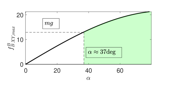
Figure 5: Radius of the maximum inscribed sphere is the feasible force set in Figure 2 for different values of $\alpha$.When this is equal to its weight, OmniMorph can sustain its weight in all orientations.

3 Control

This section introduces a control law that allows OmniMorph to follow a desired 6D trajectory switching between the underactuated and the fully actuated configurations to account for the minimization of trajectory tracking error and the minimization of the input $\bm{u}_{w}$.

Let us define $\ddot{\boldsymbol{q}}=[\ddot{\bm{p}}^{\top},\ \dot{\boldsymbol{\omega}}^{\top}]^{\top}$. Given a reference trajectory for the UAV, indicated through the superscript $(\cdot)^{d}$, we compute the reference acceleration of the robot, call it $\ddot{\boldsymbol{q}}^{r}$, using a PD feedback control plus a feedforward term. The following desired input acceleration is obtained:

$$\ddot{\boldsymbol{q}}^{r}=\begin{bmatrix}\ddot{\bm{p}}^{d}+\mathbf{K}_{p1}\dot{\bm{e}}_{p}+\mathbf{K}_{p2}\bm{e}_{p}\\ {\dot{\bm{\omega}}}^{d}+\mathbf{K}_{\omega 1}\bm{e}_{\omega}+\mathbf{K}_{\omega 2}{\bm{e}}_{R},\end{bmatrix}$$ (14)

where ${{\bm{e}}_{R}=\frac{1}{2}[\mathbf{R}^{\top}{\mathbf{R}}^{d}-{{\mathbf{R}}^{d}}^{\top}\mathbf{R}]_{\vee}}$, with _∨ from $so(3)$ to $\mathbb{R}^{3}$ being the inverse of the hat map [20], ${\bm{e}}_{p}=\bm{p}^{d}-\bm{p}$, and ${\bm{e}_{\omega}={\bm{\omega}}^{d}-\bm{\omega}}$.

We now design an inner control loop to track ${\ddot{\boldsymbol{q}}^{r}}$ thanks to suitable inputs ${\alpha^{\ast}}$ and ${\boldsymbol{u}_{w}^{\ast}},$ chosen as the solution to:

—s— α, u_w, ¨qJ_1 + J_2 + J_3 M¨q=μ+J_RF(α)u_w Cu_w¡b -ϵ_α≤α-α^∗_k-1≤ϵ_α where the cost function is composed of three terms: ${J_{1}=||\boldsymbol{u}_{w}||^{2}_{\mathbf{W}_{1}}}$ is to minimize the norm of the input, ${J_{2}=||\ddot{\boldsymbol{q}}^{r}-\ddot{\boldsymbol{q}}||_{\mathbf{W}_{2}}^{2}}$ to ensure tracking of the desired trajectory, and ${J_{3}=||\boldsymbol{u}_{w}-{\boldsymbol{u}^{*}}_{w,k-1}||^{2}_{\mathbf{W}_{3}}}$ to minimize the propeller spinning accelerations. The quantities ${\alpha^{*}}_{k-1}$ and ${\boldsymbol{u}^{*}}_{w,k-1}$ are the solution of the optimization problem (3) at the previous time step. $||\cdot||_{W_{i}}$ is the 2-norm weighted by the positive definite weight matrix $\mathbf{W}_{i}$. Alternatively, if the bounds on the propeller accelerations are identified, as in [21], $J_{3}$ could be also expressed as a unilateral constraint.

The equality constraint in (3) is the system’s dynamics, where we have indicated the inertia matrix as ${\mathbf{M}=\begin{bmatrix}m\mathbf{I}_{3}&\boldsymbol{0}_{3}\\ \boldsymbol{0}_{3}&\mathbf{J}\end{bmatrix}},$ the vector of the gravity and Coriolis terms as ${\bm{\mu}=\begin{bmatrix}-mg\bm{e}_{3}\\ -\boldsymbol{\omega}\times\mathbf{J}\boldsymbol{\omega}\end{bmatrix}},$ and $\mathbf{J}_{R}=\begin{bmatrix}\mathbf{R}&\boldsymbol{0}_{3}\\ \boldsymbol{0}_{3}&\mathbf{I}_{3}\end{bmatrix}$; the second, unilateral, constraint in (3) expresses the input constraint, where $\mathbf{C},\bm{b}$ are properly defined constant quantities; the last constraint is on the rate of change of $\alpha$. The maximum rate of change $\epsilon_{\alpha}$ is here defined as symmetric but in the general case they may also be non-symmetric and the analysis still holds.

Please note that $J_{1}$ has an equivalent effect to minimizing the norm of the drag moments, as it differs from the input norm by a constant coefficient.

In order to solve problem (3), which is not a QP problem because the first constraint is nonlinear in the optimization variables, we proceed as follows. Consider the following problem for a fixed value of $\alpha$, indicated as $\bar{\alpha}.$ —s— u_w, ¨qJ_1 + J_2 + J_3 M¨q=μ+J_RF(¯α)u_w Cu_w¡b Problem (3) is now a QP problem as $\alpha$ is not an optimization variable anymore, and, as a consequence, the bilateral constraint is linear in the optimization variables.

At each time step (3) is solved three times for three different values of $\bar{{\alpha}}=\{{\alpha^{\ast}}_{k-1}-\epsilon_{\alpha},\,{{\alpha}^{\ast}}_{k-1},\,{{\alpha}^{\ast}}_{k-1}+\epsilon_{\alpha}\}.$ Hence, at each time step, the solutions $\alpha^{\ast}$ and $\bm{u}_{w}^{\ast}$ that correspond to the lowest value of the cost function are selected. A schematic representation of the proposed control scheme is in Figure 6.

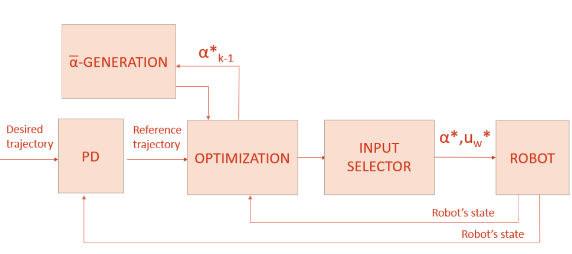
Figure 6: Block diagram of the proposed control method.

Please note that, in principle, the selection of the parameter $\bar{\alpha}\in[{\alpha}^{\ast}_{k-1}-\epsilon_{\alpha},{\alpha}^{\ast}_{k-1}+\epsilon_{\alpha}]$ may be done following different methods. Here we proposed a simple method that allows keeping the value of the tilting angle constant or changing it in the two possible directions accounting for the bound on the variation of $\alpha$. Other approaches such as an exhaustive search or more efficient sampling algorithms are possibilities, and their assessment is left for future work.

Note that, by tuning the weights $\mathbf{W}_{i}$, the control input negotiates between low input effort and low tracking error. We recall that, thanks to its redundancy, the robot is able to follow a certain desired trajectory with different values of the control inputs.

4 Simulations

Numerical simulations have been carried out using a URDF description of the OmniMorph and ODE physics engine in Gazebo. The control software has been implemented in Matlab-Simulink. The interface between Matlab and Gazebo is managed by a Gazebo-genom3 plugin. A Simulink s-function embedding qpOases QP solver has been used for the optimization problem.

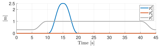
(a)

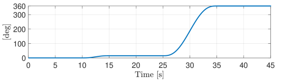
(b)

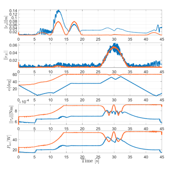
(c)

The mass and inertia of the robot are $m=1.3150\,\rm{kg}$ and ${\mathbf{J}=\rm{diag}(1.16\cdot 10^{-2},1.13\cdot 10^{-2},1.13\cdot 10^{-2})\,\rm{Nms^{2}}}$ The other parameters are

• ${\mathbf{K}_{p1}=\rm{diag}(60,60,60)}\,\rm{s^{-1}}$,

• $\mathbf{K}_{p2}=\rm{diag}(100,100,150)\,\rm{s^{-2}}$,

• ${\mathbf{K}_{\omega 1}=\rm{diag}(60,60,2)}\rm{s^{-1}}$, ${\mathbf{K}_{\omega 2}=\rm{diag}(300,300,20)}\,\rm{s^{-2}}$,

• ${\mathbf{W}_{3}=10^{-5}\mathbf{I}_{8}}$.

The tilting angle $\alpha$ is saturated at 60 deg, a value sufficient to reach the omnidirectionality, as it will be in the real robot.

We show two different simulation scenarios, let us refer to them as Case A and Case B, in which the robot’s desired trajectory is the same, but the optimization gains are different. Especially, the trajectory includes moving upwards/downwards, translating with a tilted attitude, and rotating by 360 degrees on the spot—see Figures LABEL:fig:trajp and LABEL:fig:trajR. It has been chosen to cover the whole spectrum of the actuation modes: the vertical motion with constant upward orientation is feasible in the underactuated mode, the lateral translations with constant upward orientation require full actuation, and the full 360 deg rotation on the spot about a horizontal axis requires omnidirectionality.

What distinguishes the two scenarios is that Case A is characterized by a lower weight on the input, $\mathbf{W}_{1}$, and a higher weight on the tracking error, $\mathbf{W}_{2}$, than Case B.

The optimization weights for Case A are $\mathbf{W}_{1}=10^{-8}\mathbf{I}_{8}$ and ${\mathbf{W}_{2}=\rm{diag}(3\cdot 10^{6},3\cdot 10^{6},3\cdot 10^{6},10^{3},10^{3},10^{3})}$. The optimization weights for Case B are $\mathbf{W}_{1}=10^{-5}\mathbf{I}_{8}$ and $\mathbf{W}_{2}=\rm{diag}(3\cdot 10^{4},3\cdot 10^{4},3\cdot 10^{4},1,1,1)$.

In Figure LABEL:fig:sim_results, we report a comparison between the results of the two simulation scenarios. One can appreciate as in Case A the robot performs better in terms of tracking (mean square position and attitude errors are, respectively, $0.011\,\rm{cm}$ and $0.008$), at the expenses of a higher motor torque; the tilting angle is increased and kept at the highest value along the task execution. On the contrary, in Case B, the errors are higher (mean square position and attitude errors are, respectively, $0.031\,\rm{m}$ and $0.011$), but the motor torque is, as expected, lower, and the propeller tilting angle is decreased as soon as the robot only moves vertically (as soon as the underactuated mode is enough to perform the desired motion); the efficiency is better in Case B with a total consumed energy of $1151.4\,\rm{J}$ against $2042.1\,\rm{J}$ in Case A, which guarantees an increase of the flight time of about 70%.

5 Conclusions

This work presented the design concept of OmniMorph, a novel morphing multirotor that can range between omnidirectionality and underactuation thanks to actively tilting propellers. The design leverages one single servomotor to synchronously tilt all the propellers, thus reducing the mechanical complexity and the additional payload. The dynamics model was presented, and the actuation properties depending on the propeller tilting angles were studied. Hence, a controller was proposed to negotiate between input effort and tracking performance. Simulations in a realistic Gazebo environment were presented.

In the future, experiments on the real prototype will be carried out, and predictive controllers will be tested. Equipping the OmniMorph with physical interaction capabilities in an interesting future direction.

6 Statements and Declarations

This work was partially funded by European Commission project H2020 AERIAL-CORE (871479) and MSCA project Flyflic (101059875). The authors have no relevant financial or non-financial interests to disclose.

References

- [1] A. Ollero, M. Tognon, A. Suarez, D. Lee, and A. Franchi, “Past, Present, and Future of Aerial Robotic Manipulators,” IEEE Transactions on Robotics, vol. 38, no. 1, pp. 626–645, Feb. 2022, conference Name: IEEE Transactions on Robotics.
- [2] M. Tognon, R. Alami, and B. Siciliano, “Physical Human-Robot Interaction With a Tethered Aerial Vehicle: Application to a Force-Based Human Guiding Problem,” IEEE Transactions on Robotics, vol. 37, no. 3, pp. 723–734, Jun. 2021, conference Name: IEEE Transactions on Robotics.
- [3] M. Tognon, H. A. T. Chávez, E. Gasparin, Q. Sablé, D. Bicego, A. Mallet, M. Lany, G. Santi, B. Revaz, J. Cortés et al., “A truly-redundant aerial manipulator system with application to push-and-slide inspection in industrial plants,” IEEE Robotics and Automation Letters, vol. 4, no. 2, pp. 1846–1851, 2019.
- [4] C. Gabellieri, M. Tognon, D. Sanalitro, and A. Franchi, “Equilibria, stability, and sensitivity for the aerial suspended beam robotic system subject to model uncertainty,” arXiv preprint arXiv:2302.07031, 2023.
- [5] G. Corsini, M. Jacquet, H. Das, A. Afifi, D. Sidobre, and A. Franchi, “Nonlinear model predictive control for human-robot handover with application to the aerial case,” in 2022 IEEE/RSJ International Conference on Intelligent Robots and Systems (IROS). IEEE, 2022, pp. 7597–7604.
- [6] M. Hamandi, F. Usai, Q. Sablé, N. Staub, M. Tognon, and A. Franchi, “Design of multirotor aerial vehicles: A taxonomy based on input allocation,” The International Journal of Robotics Research, vol. 40, no. 8-9, pp. 1015–1044, Aug. 2021, publisher: SAGE Publications Ltd STM. [Online]. Available: https://doi.org/10.1177/02783649211025998
- [7] M. Hamandi, Q. Sable, M. Tognon, and A. Franchi, “Understanding the omnidirectional capability of a generic multi-rotor aerial vehicle,” in 2021 Aerial Robotic Systems Physically Interacting with the Environment (AIRPHARO), Oct. 2021, pp. 1–6.
- [8] M. Hamandi, K. Sawant, M. Tognon, and A. Franchi, “Omni-Plus-Seven (O7+): An Omnidirectional Aerial Prototype with a Minimal Number of Unidirectional Thrusters,” in 2020 International Conference on Unmanned Aircraft Systems (ICUAS), Sep. 2020, pp. 754–761, iSSN: 2575-7296.
- [9] D. Brescianini and R. D’Andrea, “Design, modeling and control of an omni-directional aerial vehicle,” in 2016 IEEE International Conference on Robotics and Automation (ICRA), May 2016, pp. 3261–3266.
- [10] S. Park, J. Her, J. Kim, and D. Lee, “Design, modeling and control of omni-directional aerial robot,” in 2016 IEEE/RSJ International Conference on Intelligent Robots and Systems (IROS), Oct. 2016, pp. 1570–1575, iSSN: 2153-0866.
- [11] S. Park, J. Lee, J. Ahn, M. Kim, J. Her, G.-H. Yang, and D. Lee, “ODAR: Aerial Manipulation Platform Enabling Omnidirectional Wrench Generation,” IEEE/ASME Transactions on Mechatronics, vol. 23, no. 4, pp. 1907–1918, Aug. 2018, conference Name: IEEE/ASME Transactions on Mechatronics.
- [12] M. Tognon and A. Franchi, “Omnidirectional Aerial Vehicles With Unidirectional Thrusters: Theory, Optimal Design, and Control,” IEEE Robotics and Automation Letters, vol. 3, no. 3, pp. 2277–2282, Jul. 2018, conference Name: IEEE Robotics and Automation Letters.
- [13] M. Ryll, H. H. Bülthoff, and P. R. Giordano, “A Novel Overactuated Quadrotor Unmanned Aerial Vehicle: Modeling, Control, and Experimental Validation,” IEEE Transactions on Control Systems Technology, vol. 23, no. 2, pp. 540–556, Mar. 2015, conference Name: IEEE Transactions on Control Systems Technology.
- [14] M. Kamel, S. Verling, O. Elkhatib, C. Sprecher, P. Wulkop, Z. Taylor, R. Siegwart, and I. Gilitschenski, “The Voliro Omniorientational Hexacopter: An Agile and Maneuverable Tiltable-Rotor Aerial Vehicle,” IEEE Robotics & Automation Magazine, vol. 25, no. 4, pp. 34–44, Dec. 2018, conference Name: IEEE Robotics & Automation Magazine.
- [15] M. Allenspach, K. Bodie, M. Brunner, L. Rinsoz, Z. Taylor, M. Kamel, R. Siegwart, and J. Nieto, “Design and optimal control of a tiltrotor micro-aerial vehicle for efficient omnidirectional flight,” The International Journal of Robotics Research, vol. 39, no. 10-11, pp. 1305–1325, Sep. 2020, publisher: SAGE Publications Ltd STM. [Online]. Available: https://doi.org/10.1177/0278364920943654
- [16] M. Ryll, D. Bicego, and A. Franchi, “Modeling and control of FAST-Hex: A fully-actuated by synchronized-tilting hexarotor,” in 2016 IEEE/RSJ International Conference on Intelligent Robots and Systems (IROS), Oct. 2016, pp. 1689–1694, iSSN: 2153-0866.
- [17] M. Ryll, D. Bicego, M. Giurato, M. Lovera, and A. Franchi, “FAST-Hex—A Morphing Hexarotor: Design, Mechanical Implementation, Control and Experimental Validation,” IEEE/ASME Transactions on Mechatronics, vol. 27, no. 3, pp. 1244–1255, Jun. 2022, conference Name: IEEE/ASME Transactions on Mechatronics.
- [18] D. Brescianini and R. D’Andrea, “An omni-directional multirotor vehicle,” Mechatronics, vol. 55, pp. 76–93, Nov. 2018. [Online]. Available: https://www.sciencedirect.com/science/article/pii/S0957415818301314
- [19] G. Michieletto, M. Ryll, and A. Franchi, “Fundamental actuation properties of multirotors: Force–moment decoupling and fail–safe robustness,” IEEE Transactions on Robotics, vol. 34, no. 3, pp. 702–715, 2018.
- [20] T. Lee, M. Leok, and N. H. McClamroch, “Geometric tracking control of a quadrotor UAV on SE(3),” in 49th IEEE conference on decision and control. IEEE, 2010, pp. 5420–5425.
- [21] D. Bicego, J. Mazzetto, R. Carli, M. Farina, and A. Franchi, “Nonlinear model predictive control with enhanced actuator model for multi-rotor aerial vehicles with generic designs,” Journal of Intelligent & Robotic Systems, vol. 100, pp. 1213–1247, 2020.