Asymptotic regimes in oscillatory systems with damped non-resonant perturbations

Abstract. An autonomous system of ordinary differential equations describing nonlinear oscillations on the plane is considered. The influence of time-dependent perturbations decaying at infinity in time is investigated. It is assumed that the perturbations satisfy the non-resonance condition and do not vanish at the equilibrium of the limiting system. Possible long-term asymptotic regimes for perturbed solutions are described. In particular, we show that the perturbed system can behave like the corresponding limiting system or new asymptotically stable regimes may appear. The proposed analysis is based on the combination of the averaging technique and the construction of Lyapunov functions.

Keywords: asymptotically autonomous system, nonlinear oscillations, damped perturbations, asymptotics, stability, averaging

Mathematics Subject Classification: 34D10, 34D20, 34D05, 37J40, 70K65

Introduction

The paper is devoted to studying the effect of perturbations decaying in time on the class of autonomous systems. Such perturbed asymptotically autonomous systems arise in a wide range of problems, for example, in the study of epidemiological models [2], Painlevé equations [1], phase-locking phenomena [3], celestial motions [4], and in other problems associated with nonlinear non-autonomous systems [5, 6, 7]. Note that global properties of solutions of asymptotically autonomous systems have been studied in many papers [8, 9, 10]. In particular, it follows from [11] that, under some conditions, decaying perturbations can preserve the dynamics described by the limiting systems. See also [12], where the conditions are described under which damped perturbations do not disturb the global dynamics of autonomous oscillatory systems. In the general case, the global properties of perturbed and unperturbed trajectories can differ significantly [13, 14]. It depends both on the class of decaying perturbations and on the class of limiting systems.

In this paper, we study the effect of decaying perturbations on nonlinear oscillatory systems. It is assumed that the perturbations oscillate with an asymptotically constant frequency, satisfy the non-resonance condition, and do not preserve the equilibrium of the limiting system. Note that similar perturbations, but vanishing at the equilibrium, have been considered in several papers. For example, linear systems were considered in [15, 16, 17, 18], where the asymptotic behaviour of solutions at infinity was investigated. Bifurcations of the equilibrium and the asymptotic behaviour of perturbed solutions for the corresponding nonlinear systems were discussed in [19, 20] for both the resonant and non-resonant cases. Decaying oscillatory perturbations with increasing frequency in time were studied in [21, 22, 23, 24]. However, to the best of the author’s knowledge, damped perturbations with an asymptotically constant frequency that do not preserve equilibrium have not previously been considered in detail. In this case, difficulties arise both at the stage of choosing some analogues of fixed points and at the analysis of their stability. In this paper, we consider such perturbations in the non-resonant case and discuss long-term asymptotic regimes of solutions and their stability.

The paper is organized as follows. In Section 1, the statement of the problem is given and the class of perturbations is described. The main results are presented in Section 2. The justification is provided in the subsequent sections. In particular, in Section 3, a near-identity transformation that simplifies the system in the first asymptotic terms at infinity in time is constructed. Then, under some natural assumptions on the structure and parameters of the simplified equations, possible asymptotic regimes for solutions of the perturbed system and their stability are discussed. The justification of these results for different cases is contained in sections 4, 5 and 6. In Section 7 the proposed theory is applied to some examples of asymptotically autonomous systems. The paper concludes with a brief discussion of the results obtained.

1. Problem statement

Consider a non-autonomous system of ordinary differential equations

(1) $$\frac{dr}{dt}=f(r,\varphi,S(t),t),\quad\frac{d\varphi}{dt}=\omega(r)+r^{-1}g(r,\varphi,S(t),t),$$

where the functions $\omega(r)$, $f(r,\varphi,S,t)$ and $g(r,\varphi,S,t)$ are infinitely differentiable, defined for all $|r|\leq r_{0}={\hbox{\rm const}}$, $(\varphi,S)\in\mathbb{R}^{2}$, $t>0$, and $2\pi$-periodic with respect to $\varphi$ and $S$. It is assumed that $S(t)\sim s_{0}t$ as $t\to\infty$ with $s_{0}={\hbox{\rm const}}>0$, and for each fixed $r$ and $\varphi$

$$f(r,\varphi,S(t),t)\to 0,\quad g(r,\varphi,S(t),t)\to 0,\quad t\to\infty.$$

Hence, system (1) is asymptotically autonomous, and the limiting system is given by

(2) $$\frac{dr}{dt}=0,\quad\frac{d\varphi}{dt}=\omega(r).$$

We assume that $\omega(r)>0$ for all $|r|\leq r_{0}$. In this case, system (2) describes nonlinear oscillations on the plane $(x,y)=(r\cos\varphi,-r\sin\varphi)$ with a period $T(r)\equiv 2\pi/\omega(r)$ and an equilibrium at the origin $(0,0)$. The solutions $r(t)$ and $\varphi(t)$ of system (1) corresponds to the amplitude and the phase of oscillations. The functions $f(r,\varphi,S(t),t)$ and $r^{-1}g(r,\varphi,S(t),t)$ play the role of perturbations of system (2).

Note that system (1) in the Cartesian coordinates $(x,y)$ takes the form

$$\frac{dx}{dt}=\omega\left(r\right)y+F(x,y,t),\quad\frac{dy}{dt}=-\omega\left(r\right)x+G(x,y,t),$$

where $r=\sqrt{x^{2}+y^{2}}$, $F(x,y,t)\equiv(xf+yg)/r$ and $G(x,y,t)\equiv(yf-xg)/r$. We see that the perturbations $F(x,y,t)$ and $G(x,y,t)$ do not generally preserve the equilibrium $(0,0)$.

The goal of the paper is to study the influence of perturbations $f(r,\varphi,S(t),t)$ and $r^{-1}g(r,\varphi,S(t),t)$ on the dynamics in the vicinity of the solution $r=0$ of the limiting system and to describe possible long-term asymptotic regimes.

Let us specify the class of perturbations. We assume that

(3) $$\begin{split}&f(r,\varphi,S,t)\sim\sum_{k=1}^{\infty}t^{-\frac{k}{q}}f_{k}(r,\varphi,S),\\ &g(r,\varphi,S,t)\sim\sum_{k=1}^{\infty}t^{-\frac{k}{q}}g_{k}(r,\varphi,S),\quad t\to\infty,\end{split}$$

for all $|r|\leq r_{0}$ and $(\varphi,S)\in\mathbb{R}^{2}$, where $q\in\mathbb{Z}_{+}$ and the coefficients $f_{k}(r,\varphi,S)$, $g_{k}(r,\varphi,S)$ are $2\pi$-periodic with respect to $\varphi$ and $S$ such that their Fourier series

$$f_{k}(r,\varphi,S)=\sum_{(k_{1},k_{2})\in\mathbb{Z}^{2}}f_{k,k_{1},k_{2}}(r)e^{i(k_{1}\varphi+k_{2}S)},\quad g_{k}(r,\varphi,S)=\sum_{(k_{1},k_{2})\in\mathbb{Z}^{2}}g_{k,k_{1},k_{2}}(r)e^{i(k_{1}\varphi+k_{2}S)}$$

contain a finite number of harmonics $e^{ik_{2}S}$. Moreover, it assumed that the following condition holds:

(4) $$\begin{split}\exists\,p\in\mathbb{Z}_{+}:\quad&|f_{k}(r,\varphi,S)|+|g_{k}(r,\varphi,S)|=\mathcal{O}(r),\quad k<p,\quad f_{p,0,0}(0)\neq 0.\end{split}$$

Note that this assumption ensures that the first $p-1$ terms in the series (3) preserve the equilibrium of the limiting system. The phase of perturbations is considered in the form

(5) $$S(t)=s_{0}t+\sum_{k=1}^{q-1}s_{k}t^{1-\frac{k}{q}}+s_{q}\log t,$$

where $s_{k}={\hbox{\rm const}}$ and the parameter $s_{0}$ satisfies a non-resonance condition

(6) $$k_{1}\omega(0)+k_{2}s_{0}\neq 0\quad\forall\,k_{1},k_{2}\in\mathbb{Z},\quad|k_{1}|+|k_{2}|\neq 0.$$

Consider the example

(7) $$\frac{dx}{dt}=y,\quad\frac{dy}{dt}=-x+t^{-1}\lambda y+t^{-\frac{p}{2}}\frac{\gamma(S(t))y}{\sqrt{x^{2}+y^{2}}},$$

where $\gamma(S)=\gamma_{0}+\gamma_{1}\sin S$, $S(t)=\sqrt{2}t$, $\lambda,\gamma_{0},\gamma_{1}\in\mathbb{R}$, and $p\in\mathbb{Z}_{+}$. It can easily be checked that system (7) corresponds in the polar coordinates $x=r\cos\varphi$, $y=-r\sin\varphi$ to (1) with

$$f(r,\varphi,S,t)\equiv t^{-1}\lambda r\sin^{2}\varphi+t^{-\frac{p}{2}}\gamma(S)\sin^{2}\varphi,$$

$$g(r,\varphi,S,t)\equiv t^{-1}\lambda r\sin\varphi\cos\varphi+t^{-\frac{p}{2}}\gamma(S)\sin\varphi\cos\varphi,$$

$s_{0}=\sqrt{2}$, $\omega(r)\equiv 1$, $f_{p,0,0}(0)=\gamma_{0}/2$. If $\lambda=\gamma_{0}=\gamma_{1}=0$, system (7) has $2\pi$-periodic general solution $x(t)\equiv\rho\cos(t+\phi)$, $y(t)\equiv-\rho\sin(t+\phi)$, where $\rho$ and $\phi$ are arbitrary constants. In this case, $r(t)\equiv\rho$ and $\varphi(t)\equiv t+\phi$. In the absence of oscillating part of the perturbation ($\lambda\neq 0$, $\gamma(S)\equiv 0$), the asymptotics of the solutions can be easily constructed by using the WKB approximations [25]:

$$r(t)=\rho t^{\frac{\lambda}{2}}\left(1+\mathcal{O}(t^{-1})\right),\quad\varphi(t)=t+\phi+\mathcal{O}(t^{-1}),\quad t\to\infty.$$

Note that the global behaviour of the system in this case is determined by the sign of the parameter $\lambda$. Numerical analysis of the system with $\lambda\neq 0$, $\gamma_{0}\neq 0$ and $\gamma_{1}\neq 0$ shows that the global dynamics depends both on the value of the parameters $\lambda$, $\gamma_{0}$, $\gamma_{1}$ and on the degree of decay $p/2$ of the oscillatory part of the perturbation. In particular, if $p>2$, we see that, as in the previous case, the stability of the system depends on the sign of $\lambda$ (see Fig. 1, a). However, if $p\leq 2$, oscillatory term of damped perturbations can break the stability of the system (see Fig. 1, b, c).

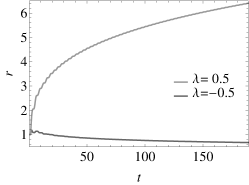
(a) $p=3$

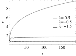
(b) $p=2$

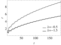
(c) $p=1$

Figure 1. The evolution of $r(t)\equiv\sqrt{x^{2}(t)+y^{2}(t)}$ for solutions to system (7) with $\gamma_{0}=\gamma_{1}=1$ and different values of the parameters $p$ and $\lambda$.

Thus, the paper investigates the role of the parameters and the structure of the considered class of damped perturbations on the qualitative and asymptotic behaviour of solutions.

2. Main results

Let us present the main results of the paper. The first of them is devoted to averaging of the system in the leading asymptotic terms and constructing the corresponding near-identity transformation.

Theorem 1.

Let system (1) satisfy (3), (4), (5) and (6). Then for all $N\in[p,2p)$ there exist $r_{\ast}\in(0,r_{0}]$, $t_{\ast}>0$ and the transformation

(8) $$\rho(t)=r(t)+\tilde{v}_{N}(r(t),\varphi(t),t),\quad\tilde{v}_{N}(r,\varphi,t)\equiv t^{-\frac{1}{q}}\tilde{v}_{N,1}(r,\varphi,t)+t^{-\frac{p}{q}}\tilde{v}_{N,p}(r,\varphi,t)$$

such that for all $|r|\leq r_{\ast}$, $\varphi\in\mathbb{R}$ and $t\geq t_{\ast}$ system (1) can be transformed into

(9) $$\frac{d\rho}{dt}=\Lambda_{N}(\rho,t)+\tilde{\Lambda}_{N}(\rho,\varphi,t),\quad\frac{d\varphi}{dt}=\omega(\rho)+\tilde{\Omega}_{N}(\rho,\varphi,t)$$

where the functions $\Lambda_{N}(\rho,t)$, $\tilde{\Lambda}_{N}(\rho,\varphi,t)$, $\tilde{\Omega}_{N}(\rho,\varphi,t)\equiv\tilde{\Omega}_{N,1}(\rho,\varphi,t)+\rho^{-1}\tilde{\Omega}_{N,p}(\rho,\varphi,t)$ are defined for all $|\rho|\leq\rho_{\ast}$, $\varphi\in\mathbb{R}$, $t\geq t_{\ast}$, $2\pi$-periodic with respect to $\varphi$, and satisfy

$$\Lambda_{N}(\rho,t)\equiv\sum_{k=1}^{N}t^{-\frac{k}{q}}\Lambda_{k}(\rho),\quad\Lambda_{k}(\rho)=\begin{cases}\mathcal{O}(|\rho|),&k<p,\\ \mu_{p}+\mathcal{O}(|\rho|),&k=p,\\ \mathcal{O}(1),&k>p,\end{cases}\quad\rho\to 0,$$

(10) $$\tilde{\Lambda}_{N}(\rho,\varphi,t)=\mathcal{O}(t^{-\frac{N+1}{q}}),\quad\tilde{\Omega}_{N,1}(\rho,\varphi,t)=\mathcal{O}(t^{-\frac{1}{q}}),\quad\tilde{\Omega}_{N,p}(\rho,\varphi,t)=\mathcal{O}(t^{-\frac{p}{q}}),\quad t\to\infty$$

uniformly for all $\varphi\in\mathbb{R}$ and $|\rho|\leq\rho_{\ast}$ with $\mu_{p}=f_{p,0,0}(0)\neq 0$. Moreover, $\tilde{v}_{N,1}(r,\varphi,t)=\mathcal{O}(|r|)$ and $\tilde{v}_{N,p}(r,\varphi,t)=\mathcal{O}(1)$ as $r\to 0$ uniformly for all $\varphi\in\mathbb{R}$ and $t\geq t_{\ast}$.

The proof is contained in Section 3.

Thus, the dynamics of system (1) is determined by the behaviour of solutions of the transformed equations. Consider some additional assumptions on the right-hand sides of system (9).

First note that the transformation described in Theorem 1 can set some terms in $\Lambda_{N}(\rho,t)$ to zero. Let $n\leq p$ be the smallest number such that

(11) $$\Lambda_{k}(\rho)\equiv 0,\quad k\leq n-1,\quad\Lambda_{n}(\rho)\not\equiv 0.$$

Along with (9), we consider the truncated system

(12) $$\frac{d\varrho}{dt}=\Lambda_{N}(\varrho,t),$$

(13) $$\frac{d\phi}{dt}=\omega(\varrho)$$

as $t\geq t_{\ast}$. This system is obtained from (9) by dropping residual terms $\tilde{\Lambda}_{N}(\rho,\varphi,t)$ and $\tilde{\Omega}_{N}(\rho,\varphi,t)$.

It can be shown that long-term regimes for solutions to system (1) are associated with the solutions of the truncated system and depend on the values of $(n,p)$.

Consider the following three cases (see Fig. 2):

$$\mathcal{Q}_{1}=\{(n,p)\in\mathbb{Z}^{2}_{+}:\quad n<p,\quad n\leq q\},$$

$$\mathcal{Q}_{2}=\{(n,p)\in\mathbb{Z}^{2}_{+}:\quad n=p,\quad n\leq q\},$$

$$\mathcal{Q}_{3}=\{(n,p)\in\mathbb{Z}^{2}_{+}:\quad n\leq p,\quad n>q\}.$$

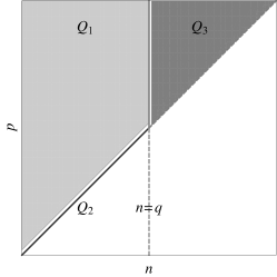
Figure 2. Partition of the parameter plane $(n,p)$.

2.1. The case $(n,p)\in\mathcal{Q}_{1}$

Assume that $\Lambda_{n}(\rho)$ has a nonzero linear part in the vicinity of the equilibrium:

(14) $$\Lambda_{n}(\rho)=\rho(\lambda_{n}+\mathcal{O}(|\rho|)),\quad\rho\to 0$$

with $\lambda_{n}={\hbox{\rm const}}\neq 0$. Define $\nu_{0}=(p-n)/q>0$. Then, we have

Lemma 1.

Let $(n,p)\in\mathcal{Q}_{1}$ and assumptions (11), (14) hold with $\lambda_{n}+\delta_{n,q}\nu_{0}<0$. Then system (12), (13) has a solution $\varrho_{1}(t)$, $\phi_{1}(t)$ such that

(15) $$\varrho_{1}(t)\sim\sum_{k=0}^{\infty}t^{-\nu_{0}-\frac{k}{q}}\rho_{k}(\log t),\quad\phi_{1}(t)\sim\omega(0)t,\quad t\to\infty,$$

where $\rho_{k}(\tau)$ are some polynomials in $\tau$ and $\rho_{0}(\tau)\equiv-{\mu_{p}}/(\lambda_{n}+\delta_{n,q}\nu_{0})$.

Moreover, the solution $\varrho_{1}(t)$ is asymptotically stable.

Lemma 2.

Let $(n,p)\in\mathcal{Q}_{1}$ and assumptions (11), (14) hold with $\lambda_{n}+\delta_{n,q}\nu_{0}<0$. Then the solution $\varrho_{1}(t)$ of equation (12) is exponentially (polynomially) stable if $n<q$ $(n=q)$.

It can be shown that the trajectories of the full system (1) behave like the solution $\varrho_{1}(t)$, $\phi_{1}(t)$ of the truncated system.

Theorem 2.

Let system (1) satisfy (3), (4), (5), (6), and $(n,p)\in\mathcal{Q}_{1}$ be integers such that assumptions (11), (14) hold with $\lambda_{n}+\delta_{n,q}\nu_{0}<0$. Then for all $\varepsilon>0$ there exist $\delta_{0}>0$ and $t_{0}\geq t_{\ast}$ such that the solution $r(t)$, $\varphi(t)$ of system (1) with initial data $|r(t_{0})-\varrho_{1}(t_{0})|\leq\delta_{0}$ and $\varphi(t_{0})\in\mathbb{R}$ satisfies

(16) $$\sup_{t\geq t_{0}}\left\{t^{\nu_{0}}|r(t)-\varrho_{1}(t)|\right\}<\varepsilon,$$

(17) $$\varphi(t)\sim\phi_{1}(t),\quad t\to\infty.$$

On the other hand, the asymptotic regime described in Lemma 1 turns out to be unstable if $\lambda_{n}+\delta_{n,q}\nu_{0}>0$. Let $\varrho_{1,M}(t)$ be a $M$th partial sum of the series (15). Then, we have

Theorem 3.

Let system (1) satisfy (3), (4), (5), (6), and $(n,p)\in\mathcal{Q}_{1}$ be integers such that assumptions (11), (14) hold with $\lambda_{n}+\delta_{n,q}\nu_{0}>0$. Then for all $M\in\mathbb{Z}_{+}$ there exists $\varepsilon>0$ such that for all $\delta_{0}\in(0,\varepsilon)$ the solution $r(t)$, $\varphi(t)$ of system (1) with initial data $|r(t_{s})-\varrho_{1,M}(t_{s})|\leq\delta_{0}$, $\varphi(t_{s})\in\mathbb{R}$ at some $t_{s}\geq t_{\ast}$ satisfies the inequality $t_{e}^{\nu_{0}}|r(t_{e})-\varrho_{1,M}(t_{e})|\geq\varepsilon$ at some $t_{e}>t_{s}$.

Note that if $n=q$ and $\lambda_{n}<0$, it can be shown that solutions of system (1) with small enough initial amplitude will remain close to zero.

Theorem 4.

Let system (1) satisfy (3), (4), (5), (6), and $(n,p)\in\mathcal{Q}_{1}$ be integers such that assumptions (11), (14) hold with $n=q$ and $\lambda_{n}<0$. Then for all $\varepsilon>0$ there exist $\delta_{0}>0$ and $t_{0}\geq t_{\ast}$ such that the solution $r(t)$, $\varphi(t)$ of system (1) with initial data $|r(t_{0})|\leq\delta_{0}$ and $\varphi(t_{0})\in\mathbb{R}$ satisfies the inequality $|r(t)|<\varepsilon$ for all $t\geq t_{0}$.

Now, consider the case, when $\Lambda_{n}(\rho)$ is strongly nonlinear as $\rho\to 0$:

(18) $$\exists\,d,m\in\mathbb{Z}_{+}:\quad m\geq 2,\quad\Lambda_{k}(\rho)=\begin{cases}\rho^{m}(\lambda_{n,m}+\mathcal{O}(|\rho|)),&k=n,\\ \mathcal{O}(|\rho|^{m}),&k<n+d,\\ \rho(\lambda_{n+d}+\mathcal{O}(|\rho|)),&k=n+d,\end{cases}$$

with $\lambda_{n,m},\lambda_{n+d}={\hbox{\rm const}}\neq 0$. Define the parameters

$$m_{\ast}=\frac{p-n}{p-(n+d)},\quad\vartheta_{m}=\begin{cases}\displaystyle\frac{p-n}{qm},&m\leq m_{\ast},\\ \displaystyle\frac{d}{q(m-1)},&m>m_{\ast},\end{cases}$$

and the function

$$\mathcal{P}(z)\equiv\begin{cases}\displaystyle\lambda_{n,m}z^{m}+\mu_{p},&m<m_{\ast},\\ \displaystyle\lambda_{n,m}z^{m}+(\lambda_{n+d}+\delta_{n+d,q}\vartheta_{m})z+\mu_{p},&m=m_{\ast},\\ \displaystyle\lambda_{n,m}z^{m}+(\lambda_{n+d}+\delta_{n+d,q}\vartheta_{m})z,&m>m_{\ast}.\end{cases}$$

Assume that

(19) $$\exists\,z_{m}\in\mathbb{R}:\quad\mathcal{P}(z_{m})=0,\quad\mathcal{P}^{\prime}(z_{m})\neq 0.$$

Then, we have the following:

Lemma 3.

Let $(n+d,p)\in\mathcal{Q}_{1}$ and assumptions (11), (18), (19) hold with $\mathcal{P}^{\prime}(z_{m})<0$. Then system (12), (13) has a solution $\varrho_{m}(t)$, $\phi_{m}(t)$ such that

(20) $$\varrho_{m}(t)\sim\sum_{k=0}^{\infty}t^{-\vartheta_{m}-\frac{k}{qm}}\rho_{k}(\log t),\quad\phi_{m}(t)\sim\omega(0)t,\quad t\to\infty,$$

where $\rho_{k}(\tau)$ are some polynomials in $\tau$ and $\rho_{0}(\tau)\equiv z_{m}$.

Theorem 5.

Let system (1) satisfy (3), (4), (5), (6), and $(n+d,p)\in\mathcal{Q}_{2}$ be integers such that assumptions (11), (18), (19) hold with $\mathcal{P}^{\prime}(z_{m})<0$. Then for all $\varepsilon>0$ there exist $\delta_{0}>0$ and $t_{0}\geq t_{\ast}$ such that the solution $r(t)$, $\varphi(t)$ of system (1) with initial data $|r(t_{0})-\varrho_{m}(t_{0})|\leq\delta_{0}$ and $\varphi(t_{0})\in\mathbb{R}$ satisfies

$$\sup_{t\geq t_{0}}\left\{t^{\vartheta_{m}}|r(t)-\varrho_{m}(t)|\right\}<\varepsilon,\quad\varphi(t)\sim\phi_{m}(t),\quad t\to\infty.$$

The proofs of Lemmas 1, 2, 3 and Theorems 2, 3, 4 and 5 are contained in Section 4.

2.2. The case $(n,p)\in\mathcal{Q}_{2}$

In this case, the global behaviour of solutions is determined by the zeros of the coefficient $\Lambda_{p}(\rho)$. Consider the following assumption:

(21) $$\exists\,\rho_{0}\in\mathbb{R}:\quad 0<|\rho_{0}|<r_{\ast},\quad\Lambda_{p}(\rho_{0})=0,\quad\Lambda_{p}^{\prime}(\rho_{0})\neq 0.$$

Then, we have the following:

Lemma 4.

Let $(n,p)\in\mathcal{Q}_{2}$ and assumptions (11), (21) hold with $\Lambda_{p}^{\prime}(\rho_{0})<0$. Then system (12), (13) has a solution $\varrho_{2}(t)$, $\phi_{2}(t)$ such that

(22) $$\varrho_{2}(t)\sim\rho_{0}+\sum_{k=1}^{\infty}t^{-\frac{k}{q}}\rho_{k}(\log t),\quad\phi_{2}(t)\sim\omega(\rho_{0})t,\quad t\to\infty,$$

where $\rho_{k}(\tau)$ are some polynomials in $\tau$.

As in the previous case, the solution $\varrho_{2}(t)$ is asymptotically stable.

Lemma 5.

Let $(n,p)\in\mathcal{Q}_{2}$ and assumptions (11), (21) hold with $\Lambda_{p}^{\prime}(\rho_{0})<0$. Then the solution $\varrho_{2}(t)$ of equation (12) is exponentially (polynomially) stable if $p<q$ $(p=q)$.

Thus, we have

Theorem 6.

Let system (1) satisfy (3), (4), (5), (6), and $(n,p)\in\mathcal{Q}_{2}$ be integers such that assumptions (11), (21) hold with $\Lambda_{p}^{\prime}(\rho_{0})<0$. Then for all $\varepsilon>0$ and $\varkappa\in(0,|\Lambda_{p}^{\prime}(\rho_{0})|)$ there exist $\delta_{0}>0$ and $t_{0}\geq t_{\ast}$ such that the solution $r(t)$, $\varphi(t)$ of system (1) with initial data $|r(t_{0})-\varrho_{2}(t_{0})|\leq\delta_{0}$ and $\varphi(t_{0})\in\mathbb{R}$ satisfies

(23) $$\sup_{t\geq t_{0}}\left\{t^{\varkappa}|r(t)-\varrho_{2}(t)|\right\}<\varepsilon,$$

(24) $$\varphi(t)\sim\phi_{2}(t),\quad t\to\infty.$$

Note that, if $\Lambda_{p}^{\prime}(\rho_{0})>0$, the solution is unstable. Let $\varrho_{2,M}(t)$ be a $M$th partial sum of the series (22). We have the following:

Theorem 7.

Let system (1) satisfy (3), (4), (5), (6), and $(n,p)\in\mathcal{Q}_{2}$ be integers such that assumptions (11), (21) hold with $\Lambda_{p}^{\prime}(\rho_{0})>0$. Then for all $M\in\mathbb{Z}_{+}$ there exists $\varepsilon>0$ such that for all $\delta_{0}\in(0,\varepsilon)$ the solution of system (1) with initial data $|r(t_{s})-\varrho_{2,M}(t_{s})|\leq\delta_{0}$, $\varphi(t_{s})\in\mathbb{R}$ at some $t_{s}\geq t_{\ast}$ satisfies the inequality $t_{e}^{\nu_{0}}|r(t_{e})-\varrho_{2,M}(t_{e})|\geq\varepsilon$ at some $t_{e}>t_{s}$.

Consider the case when, instead of (21), the following assumption holds:

(25) $$\Lambda_{p}(\rho)\neq 0\quad\forall|\rho|<r_{\ast}.$$

Then, the solutions of system (1) exit from a neighbourhood of the equilibrium of the limiting system.

Theorem 8.

Let system (1) satisfy (3), (4), (5), (6), and $(n,p)\in\mathcal{Q}_{2}$ be integers such that assumptions (11), (25) hold. Then there exist $\varepsilon\in(0,r_{\ast})$ such that for all $\delta_{0}>0$ the solution $r(t)$, $\varphi(t)$ of system (1) with initial data $|r(t_{s})|\leq\delta_{0}$ and $\varphi(t_{s})\in\mathbb{R}$ at some $t_{s}\geq t_{\ast}$ satisfies $|r(t_{e})|\geq\varepsilon$ at some $t_{e}>t_{s}$.

The justification of Lemmas 4, 5 and Theorem 6, 7 and 8 is contained in Section 5.

2.3. The case $(n,p)\in\mathcal{Q}_{3}$

It can be shown that if $(n,p)\in\mathcal{Q}_{3}$, the amplitude of solutions can tend to any $\rho_{0}\in\mathbb{R}$ such that

(26) $$0<|\rho_{0}|<r_{\ast},\quad\Lambda_{n}(\rho_{0})\neq 0,\quad\Lambda_{n}^{\prime}(\rho_{0})\neq 0.$$

We have

Lemma 6.

Let $(n,p)\in\mathcal{Q}_{3}$ and assumption (11) hold. Then, for all $\rho_{0}\in\mathbb{R}$ satisfying (26) with $\Lambda_{n}^{\prime}(\rho_{0})<0$ there exists a solution $\varrho_{3}(t)$, $\phi_{3}(t)$ of system (12), (13) such that

(27) $$\varrho_{3}(t)\sim\rho_{0}+\sum_{k=1}^{\infty}t^{-\frac{n-q+k-1}{q}}\rho_{k},\quad\phi_{3}(t)\sim\omega(\rho_{0})t,\quad t\to\infty,$$

where $\rho_{k}={\hbox{\rm const}}$.

In contrast to the previous cases, the solution $\varrho_{3}(t)$ turns out to be only neutrally stable.

Lemma 7.

Let $(n,p)\in\mathcal{Q}_{3}$ and assumptions (11), (26) hold with $\Lambda_{p}^{\prime}(\rho_{0})<0$. Then the solution $\varrho_{2}(t)$ of equation (12) is stable.

Thus, we have the following:

Theorem 9.

Let system (1) satisfy (3), (4), (5), (6), and $(n,p)\in\mathcal{Q}_{3}$ be integers such that assumptions (11), (26) hold with $\Lambda_{n}^{\prime}(\rho_{0})<0$. Then for all $\varepsilon>0$ there exist $\delta_{0}>0$ and $t_{0}\geq t_{\ast}$ such that the solution $r(t)$, $\varphi(t)$ of system (1) with initial data $|r(t_{0})-\varrho_{3}(t_{0})|\leq\delta_{0}$ and $\varphi(t_{0})\in\mathbb{R}$ satisfies

(28) $$\sup_{t\geq t_{0}}|r(t)-\varrho_{3}(t)|<\varepsilon,$$

(29) $$\varphi(t)\sim\phi_{3}(t),\quad t\to\infty.$$

The proofs of Lemmas 6, 7 and Theorem 9 are contained in Section 6.

3. Transformation of variables

To simplify the first equation in system (1), consider the transformation of the amplitude $r$ in the following form:

(30) $$V_{N}(r,\varphi,t)\equiv r+\sum_{k=1}^{N}t^{-\frac{k}{q}}v_{k}(r,\varphi,S(t)),$$

where the coefficients $v_{k}(r,\phi,S(t))$ are sought in such a way that the equation for the new variable

(31) $$\rho(t)\equiv V_{N}(r(t),\varphi(t),S(t),t)$$

does not depend on the ‘‘fast’’ angle variables $\varphi$ and $S$ at least in the first $N\in[p,2p)$ terms of its asymptotics as $t\to\infty$. Note that such transformations are usually used in perturbation theory with a small parameter [26, 27, 28]. Differentiating both sides of (31) with respect to $t$ and taking into account (3), we obtain

$$\frac{d\rho}{dt}\sim \sum_{k=1}^{\infty}t^{-\frac{k}{q}}\left(\big{(}\omega(r)\partial_{\varphi}+s_{0}\partial_{S}\big{)}v_{k}(r,\varphi,S)+f_{k}(r,\varphi,S)+\left(1-\frac{k}{q}\right)v_{k-q}(r,\varphi,S)\right)$$

$$+\sum_{k=2}^{\infty}t^{-\frac{k}{q}}\sum_{i+j=k}\left(f_{i}(r,\varphi,S)\partial_{r}+r^{-1}g_{i}(r,\varphi,S)\partial_{\varphi}+\left(1-\frac{i}{q}\right)s_{i}\partial_{S}\right)v_{j}(r,\varphi,S)$$

as $t\to\infty$, where it is assumed that $v_{i}(r,\varphi,S)\equiv 0$ if $i<1$ or $i>N$, and $s_{j}=0$ if $j>q$. Comparing asymptotics for $dR/dt$ with the right-hand side of the first equation in (9), we get the following chain of equations:

(32) $$\big{(}\omega(r)\partial_{\varphi}+s_{0}\partial_{S}\big{)}v_{k}=\mathcal{F}_{k}(r,\varphi,S),\quad k=1,\dots,N,$$

where $\mathcal{F}_{k}(r,\varphi,S)\equiv\Lambda_{k}(r)-f_{k}(r,\varphi,S)+\mathcal{R}_{k}(r,\varphi,S)$. Note that each function $\mathcal{R}_{k}(r,\varphi,S)$ is $2\pi$-periodic with respect to $\varphi$ and $S$, and is defined through $\{v_{j}(r,\varphi,S)\}_{j=1}^{k-1}$. For instance,

$$\mathcal{R}_{1} \equiv 0,$$

$$\mathcal{R}_{2} \equiv v_{1}\partial_{r}\Lambda_{1}-\left(1-\frac{2}{q}\right)v_{2-q}-\left(f_{1}\partial_{r}+r^{-1}g_{1}\partial_{\varphi}+\left(1-\frac{1}{q}\right)s_{1}\partial_{S}\right)v_{1},$$

$$\mathcal{R}_{3} \equiv \sum_{i+j=3}v_{i}\partial_{r}\Lambda_{j}+\frac{v_{1}^{2}}{2}\partial_{r}^{2}\Lambda_{1}-\left(1-\frac{3}{q}\right)v_{3-q}-\sum_{i+j=3}\left(f_{i}\partial_{r}+r^{-1}g_{i}\partial_{\varphi}+\left(1-\frac{1}{q}\right)s_{i}\partial_{S}\right)v_{j},$$

$$\mathcal{R}_{k} \equiv \sum_{m_{1}+2m_{2}+\dots+im_{i}+j=k}C_{i,j,m_{1},\dots,m_{i}}v_{1}^{m_{1}}\cdots v_{i}^{m_{i}}\partial_{r}^{m_{1}+\dots+m_{i}}\Lambda_{j}$$

$$-\left(1-\frac{k}{q}\right)v_{k-q}-\sum_{i+j=k}\left(f_{i}\partial_{r}+r^{-1}g_{i}\partial_{\varphi}+\left(1-\frac{1}{q}\right)s_{i}\partial_{S}\right)v_{j},$$

where $C_{i,j,m_{1},\dots,m_{i}}={\hbox{\rm const}}$. Define

$$\Lambda_{k}(r)\equiv\langle f_{k}(r,\varphi,S)-\mathcal{R}_{k}(r,\varphi,S)\rangle_{\varphi,S},$$

where the angle brackets denote averaging over $\varphi$ and $S$:

$$\langle Z(\varphi,S)\rangle_{\varphi,S}:=\frac{1}{(2\pi)^{2}}\int\limits_{0}^{2\pi}\int\limits_{0}^{2\pi}Z(\varphi,S)\,d\varphi\,dS.$$

In this case, each function $\mathcal{F}_{k}(r,\varphi,S)$ is $2\pi$-periodic with respect to $\varphi$ and $S$ with zero mean. Moreover, $\mathcal{F}_{k}(r,\varphi,S)$ is expanded in Fourier series

$$\mathcal{F}_{k}(r,\varphi,S)=\sum_{|k_{1}|+|k_{2}|\neq 0}\mathcal{F}_{k,k_{1},k_{2}}(r)e^{i(k_{1}\varphi+k_{2}S)},$$

$$\mathcal{F}_{k,k_{1},k_{2}}(r)=\frac{1}{(2\pi)^{2}}\int\limits_{0}^{2\pi}\int\limits_{0}^{2\pi}\mathcal{F}_{k}(r,\varphi,S)e^{-i(k_{1}\varphi+k_{2}S)}\,d\varphi\,dS.$$

From the properties of the class of perturbations $f$ and $g$ it follows that the Fourier series of $\mathcal{F}_{k}(r,\varphi,S)$ contain a finite number of modes $e^{ik_{2}S}$. In other words, the set $\mathcal{Z}:=\{k_{2}\in\mathbb{Z}:\mathcal{F}_{k,k_{1},k_{2}}(r)\not\equiv 0,\ \ \forall\,k,k_{1}\in\mathbb{Z}\}$ is finite. Define the domain

$$\mathcal{D}:=\{|r|\leq r_{0}:\ \ k_{1}\omega(r)+k_{2}s_{0}\neq 0,\quad\forall\,k_{1}\in\mathbb{Z},\quad k_{2}\in\mathcal{Z}:\quad|k_{1}|+|k_{2}|\neq 0\}.$$

It follows from (6) that there exists $r_{\ast}\in(0,r_{0})$ such that $[-r_{\ast},r_{\ast}]\subset\mathcal{D}$. Hence, $\mathcal{D}$ is non-empty, and for all $r\in\mathcal{D}$ the solution of (32) is expanded in the Fourier series

$$v_{k}(r,\varphi,S)=\sum_{\begin{subarray}{c}k_{1}\in\mathbb{Z},k_{2}\in\mathcal{Z}\\ |k_{1}|+|k_{2}|\neq 0\end{subarray}}\frac{\mathcal{F}_{k,k_{1},k_{2}}(r)}{i(k_{1}\omega(r)+k_{2}s_{0})}e^{i(k_{1}\varphi+k_{2}S)}.$$

Thus, system (32) is solvable in the class of $2\pi$-periodic functions in $\varphi$ and $S$ with zero mean. It can easily be checked that

$$\begin{split}&\mathcal{R}_{k}(r,\varphi,S)=\begin{cases}\mathcal{O}(r),&k\leq p,\\ \mathcal{O}(1),&p<k\leq N,\end{cases}\quad\Lambda_{k}(r)=\begin{cases}\mathcal{O}(r),&k<p,\\ \mathcal{O}(1),&p\leq k\leq N,\end{cases}\\ &v_{k}(r,\varphi,S)=\begin{cases}\mathcal{O}(r),&k<p,\\ \mathcal{O}(1),&p\leq k\leq N,\end{cases}\end{split}$$

as $r\to 0$ uniformly for all $(\varphi,S)\in\mathbb{R}^{2}$. In particular, $\Lambda_{p}(r)=\langle f_{p}(0,\varphi,S)\rangle_{\varphi,S}+\mathcal{O}(r)$ as $r\to 0$.

It follows from (30) that for all $\epsilon\in(0,r_{\ast})$ there exists $t_{\ast}\geq t_{0}$ such that

$$|V_{N}(r,\varphi,t)-r|\leq\epsilon,\quad|\partial_{r}V_{N}(r,\varphi,t)-1|\leq\epsilon$$

for all $|r|\leq r_{\ast}$, $\varphi\in\mathbb{R}$ and $t\geq t_{\ast}$. Hence, the transformation $(r,\varphi,t)\mapsto(\rho,\varphi,t)$ is invertible for all $|\rho|\leq\rho_{\ast}$, $\varphi\in\mathbb{R}$ and $t\geq t_{\ast}$ with $\rho_{\ast}=r_{\ast}-\epsilon$. Denote by $r=R(\rho,\varphi,t)$ the corresponding inverse transformation. Hence,

$$\tilde{\Lambda}_{N}(\rho,\varphi,t)\equiv\Big{(}f\partial_{r}+(\omega+r^{-1}g)\partial_{\varphi}+\partial_{t}\Big{)}V_{N}\Big{|}_{r=R(\rho,\varphi,t)}-\Lambda_{N}(\rho,t),$$

$$\tilde{\Omega}_{N,1}(\rho,\varphi,t)\equiv\omega(R(\rho,\varphi,t))-\omega(\rho)+r^{-1}\sum_{k=1}^{p-1}t^{-\frac{k}{q}}g_{k}(R(\rho,\varphi,t),\varphi,S(t),t),$$

$$\tilde{\Omega}_{N,p}(\rho,\varphi,t)\equiv r^{-1}g(R(\rho,\varphi,t),\varphi,S(t),t)-r^{-1}\sum_{k=1}^{p-1}t^{-\frac{k}{q}}g_{k}(R(\rho,\varphi,t),\varphi,S(t),t).$$

Combining this with (4), we obtain (10).

Thus, we obtain the proof of Theorem 1 with $\tilde{v}_{N}(r,\varphi,t)\equiv V_{N}(r,\varphi,t)-r$,

$$\tilde{v}_{N,1}(r,\varphi,t)\equiv\sum_{k=1}^{p-1}t^{-\frac{k-1}{q}}v_{k}(r,\varphi,S(t)),\quad\tilde{v}_{N,p}(r,\varphi,t)\equiv\sum_{k=p}^{N}t^{-\frac{k-p}{q}}v_{k}(r,\varphi,S(t)).$$

4. The case $(n,p)\in\mathcal{Q}_{1}$

4.1. Proof of Lemma 1

Substituting $\varrho(t)=t^{-\nu_{0}}\xi(t)$ into equation (12) yields

(33) $$\frac{d\xi}{dt}=A_{N}(\xi,t),\quad A_{N}(\xi,t)\equiv t^{\nu_{0}}\Lambda_{N}\left(t^{-\nu_{0}}\xi,t\right)+\nu_{0}t^{-1}\xi.$$

It can easily be checked that the function $A(\xi,t)$ has the following asymptotics:

$$A_{N}(\xi,t)\sim\sum_{k=n}^{\infty}t^{-\frac{k}{q}}a_{k}(\xi),\quad t\to\infty,\quad a_{n}(\xi)\equiv\mu_{p}+(\lambda_{n}+\delta_{n,q}\nu_{0})\xi.$$

Consider a particular solution of (33) tending to a root $\xi_{0}$ of the equation $a_{n}(\xi_{0})=0$.

If $n<q$, the asymptotics for a solution of equation (33) can be constructed in the form of power series with constant coefficients:

$$\xi(t)=\xi_{0}+\sum_{k=1}^{\infty}t^{-\frac{k}{q}}\xi_{k},\quad\xi_{0}=-\frac{\mu_{p}}{\lambda_{n}},\quad\xi_{k}={\hbox{\rm const}}.$$

Substituting these series into (33) and grouping the terms of the same power of $t$ yield the following chain of equations for the coefficients $\xi_{k}$:

(34) $$-\lambda_{n}\xi_{k}=b_{k}(\xi_{0},\xi_{1},\dots,\xi_{k-1}),\quad k\geq 1,$$

where the right-hand sides $b_{k}$ are certain polynomial functions of $(\xi_{1},\dots,\xi_{k-1})$. In particular, $b_{1}\equiv a_{n+1}(\xi_{0})$, $b_{2}\equiv a_{n+2}(\xi_{0})+a_{n+1}^{\prime}(\xi_{0})\xi_{1}+a_{n}^{\prime\prime}(\xi_{0})\xi_{1}^{2}/2$. Since $\lambda_{n}\neq 0$, system (34) is solvable.

To prove the existence of a solution to equation (33) with such asymptotic expansion, consider the function

$$\xi_{M}(t)\equiv\sum_{k=0}^{M}t^{-\frac{k}{q}}\xi_{k}$$

with some $M\in\mathbb{Z}_{+}$. It can easily be checked that

$$\frac{d\xi_{M}(t)}{dt}-A_{N}(\xi_{M}(t),t)=\mathcal{O}\left(t^{-\frac{M+n+2}{q}}\right),\quad t\to\infty.$$

Substituting $\xi(t)=\xi_{M}(t)+t^{-{M}/{q}}z(t)$ into equation (33), we obtain

(35) $$\frac{dz}{dt}=\mathcal{A}(t)z+\mathcal{B}(z,t)+\mathcal{C}(t),$$

where

$$\mathcal{A}(t) \equiv\partial_{\xi}A_{N}(\xi_{M}(t),t)+\frac{M}{q}t^{-1},$$

$$\mathcal{B}(z,t) \equiv t^{\frac{M}{q}}\left[A_{N}(\xi_{M}(t)+t^{-\frac{M}{q}}z,t)-A_{N}(\xi_{M}(t),t)\right]-\partial_{\xi}A_{N}(\xi_{M}(t),t)z,$$

$$\mathcal{C}(t) \equiv t^{\frac{M}{q}}\left[A_{N}(\xi_{M}(t),t)-\frac{d\xi_{M}(t)}{dt}\right].$$

We see that

(36) $$\mathcal{A}(t)=t^{-\frac{n}{q}}\left(\lambda_{n}+\mathcal{O}(t^{-\frac{1}{q}})\right),\quad\mathcal{B}(z,t)=\mathcal{O}(z^{2})\mathcal{O}(t^{-\frac{n+M+1}{q}}),\quad\mathcal{C}(t)=\mathcal{O}(t^{-\frac{n+2}{q}})$$

as $t\to\infty$ uniformly for all $|z|\leq\zeta_{\ast}$ with some $\zeta_{\ast}={\hbox{\rm const}}>0$. Note that if $\mathcal{C}(t)\equiv 0$, equation (35) has the trivial solution $z(t)\equiv 0$. Hence, the function $\mathcal{C}(t)$ plays the role of an external perturbation. Let us prove the stability of the trivial solution with respect to this perturbation. Using $U(z)=|z|$ as a Lyapunov function candidate for equation (35), we obtain

(37) $$\frac{dU}{dt}=\mathcal{A}(t)|z|+\left(\mathcal{B}(z,t)+\mathcal{C}(t)\right){\hbox{\rm sgn }}z.$$

It follows from (36) that there exist $t_{1}\geq t_{\ast}$ and $\zeta_{1}\in(0,\zeta_{\ast})$ such that

$$\mathcal{A}(t)\leq-t^{-\frac{n}{q}}\frac{|\lambda_{n}|}{2},\quad|\mathcal{B}(z,t)|\leq t^{-\frac{n}{q}}\frac{|\lambda_{n}|}{4}|z|,\quad\mathcal{C}(t)\leq t^{-\frac{n+1}{q}}\mathcal{C}_{0}$$

for all $t\geq t_{1}$ and $|z|\leq\zeta_{1}$ with some $\mathcal{C}_{0}={\hbox{\rm const}}>0$. Moreover, for all $\varepsilon\in(0,\zeta_{1})$ there exist

$$\delta_{\varepsilon}=\frac{8\mathcal{C}_{0}t_{\varepsilon}^{-\frac{1}{q}}}{|\lambda_{n}|}<\varepsilon,\quad t_{\varepsilon}=\max\left\{t_{1},\left(\frac{16\mathcal{C}_{0}}{\varepsilon|\lambda_{n}|}\right)^{q}\right\}$$

such that

$$\frac{dU}{dt}\leq t^{-\frac{n}{q}}\left(-\frac{|\lambda_{n}|}{4}+t_{\varepsilon}^{-\frac{1}{q}}\frac{\mathcal{C}_{0}}{\delta_{\varepsilon}}\right)U\leq-t^{-\frac{n}{q}}\frac{|\lambda_{n}|}{8}U<0$$

for all $\delta_{\varepsilon}\leq|z|\leq\varepsilon$ and $t\geq t_{\varepsilon}$. Combining this with the inequalities

(38) $$\sup_{|z|\leq\delta_{\varepsilon}}U(z)\leq\delta_{\varepsilon}<\varepsilon=\inf_{|z|=\varepsilon}U(z),$$

we see that any solution $z(t)$ of equation (35) with initial data $|z(t_{\varepsilon})|\leq\delta_{\varepsilon}$ cannot exit from the domain $|z|\leq\varepsilon$ as $t\geq t_{\varepsilon}$. Hence, for all $M\in\mathbb{Z}_{+}$ the solutions $\xi_{\ast}(t)$ of equation (33) starting in the vicinity of $\xi_{0}$ satisfy the estimate $\xi_{\ast}(t)=\xi_{M}(t)+\mathcal{O}(t^{-\frac{M}{q}})$ as $t\to\infty$. Returning to the original variables, we obtain the existence of the solution $\varrho_{1}(t)=t^{-\nu_{0}}\xi_{\ast}(t)$ with asymptotics (15), where $\rho_{k}(\tau)\equiv\xi_{k}$. Note that similar method for justifying asymptotic expansions at infinity was used in [29] for the case when the corresponding linearised system has negative eigenvalues.

Consider now the case $n=q$. In this case, the asymptotic solution is constructed in the form (see [5])

(39) $$\xi(t)=\xi_{0}+\sum_{k=1}^{\infty}t^{-\frac{k}{q}}\xi_{k}(\log t),\quad\xi_{0}=-\frac{\mu_{p}}{\lambda_{n}+\nu_{0}},$$

where the coefficients $\xi_{k}(\tau)$ depend polynomially on $\tau$. Substituting (39) into (33), we obtain the chain of differential equations

(40) $$\frac{d\xi_{k}}{d\tau}-\left(\lambda_{n}+\nu_{0}+\frac{k}{q}\right)\xi_{k}=b_{k}(\xi_{0},\xi_{1},\dots,\xi_{k-1}),\quad k\geq 1.$$

Since $\lambda_{n}+\nu_{0}<0$, it follows that system (40) is solvable and

$$\xi_{k}(\tau)\equiv\begin{cases}\displaystyle-\frac{b_{k}(\xi_{0},\xi_{1}(\tau),\dots,\xi_{k-1}(\tau))}{\lambda_{n}+\nu_{0}+k/q},&\displaystyle k<q|\lambda_{n}+\nu_{0}|,\\ \displaystyle\int\limits_{\log t_{\ast}}^{\tau}b_{k}(\xi_{0},\xi_{1}(\theta),\dots,\xi_{k-1}(\theta))\,d\theta,&\displaystyle k=q|\lambda_{n}+\nu_{0}|,\\ \displaystyle\int\limits_{\infty}^{\tau}e^{-(\lambda_{n}+\nu_{0}+k/q)(\theta-\tau)}b_{k}(\xi_{0},\xi_{1}(\theta),\dots,\xi_{k-1}(\theta))\,d\theta,&\displaystyle k>q|\lambda_{n}+\nu_{0}|.\end{cases}$$

Define the function

$$\xi_{M}(t)\equiv\xi_{0}+\sum_{k=1}^{M}t^{-\frac{k}{q}}\xi_{k}(\log t),\quad M\in\mathbb{Z}_{+}.$$

It is readily seen that in this case

$$\frac{d\xi_{M}(t)}{dt}-A_{N}(\xi_{M}(t),t)=\mathcal{O}\left(t^{-1-\frac{M+1}{q}}\right),\quad t\to\infty.$$

Substituting $\xi(t)=\xi_{M}(t)+z(t)$ into (33), we get (35) but with the functions

$${\mathcal{A}}(t) \equiv\partial_{\xi}A_{N}(\xi_{M}(t),t),$$

$${\mathcal{B}}(z,t) \equiv A_{N}(\xi_{M}(t)+z,t)-A_{N}(\xi_{M}(t),t)-\partial_{\xi}A_{N}(\xi_{M}(t),t)z,$$

$${\mathcal{C}}(t) \equiv A_{N}(\xi_{M}(t),t)-\frac{d\xi_{M}(t)}{dt}$$

that satisfy the estimates

(41) $${\mathcal{A}}(t)=t^{-1}\left(-|\lambda_{n}+\nu_{0}|+\mathcal{O}(t^{-\frac{1}{q}})\right),\quad{\mathcal{B}}(z,t)=\mathcal{O}(z^{2})\mathcal{O}(t^{-1-\frac{1}{q}}),\quad{\mathcal{C}}(t)=\mathcal{O}(t^{-1-\frac{M+1}{q}})$$

as $t\to\infty$ uniformly for all $|z|\leq\zeta_{\ast}$ with some $\zeta_{\ast}={\hbox{\rm const}}>0$. As in the previous case, we take $U(z)=|z|$ as a Lyapunov function candidate. In this case, we see that for all $\epsilon\in(0,1)$ there exist $t_{1}\geq t_{\ast}$ and $\zeta_{1}\in(0,\zeta_{\ast})$ such that

(42) $${\mathcal{A}}(t)\leq-t^{-1}\frac{|\lambda_{n}+\nu_{0}|}{2},\quad|{\mathcal{B}}(z,t)|\leq t^{-1}\frac{|\lambda_{n}+\nu_{0}|}{4}|z|,\quad{\mathcal{C}}(t)\leq t^{-1-\frac{M+1}{q}}\mathcal{C}_{0}$$

for all $t\geq t_{1}$ and $|z|\leq\zeta_{1}$ with some $\mathcal{C}_{0}={\hbox{\rm const}}>0$. Hence, for all $\varepsilon\in(0,\zeta_{1})$ there exist

$$\delta_{\varepsilon}=\frac{8\mathcal{C}_{0}t_{\varepsilon}^{-\frac{M+1}{q}}}{|\lambda_{n}+\nu_{0}|}<\varepsilon,\quad t_{\varepsilon}=\max\left\{t_{1},\left(\frac{16\mathcal{C}_{0}}{\varepsilon|\lambda_{n}+\nu_{0}|}\right)^{\frac{q}{M+1}}\right\}$$

such that

$$\frac{dU}{dt}\leq t^{-1}\left(-\frac{|\lambda_{n}+\nu_{0}|}{4}+t_{\varepsilon}^{-\frac{M+1}{q}}\frac{\mathcal{C}_{0}}{\delta_{\varepsilon}}\right)U\leq-t^{-1}\frac{|\lambda_{n}+\nu_{0}|}{8}U<0$$

for all $\delta_{\varepsilon}\leq|z|\leq\varepsilon$ and $t\geq t_{\varepsilon}$. Combining this with (38), we see that any solution $z(t)$ of equation (35) with initial data $|z(t_{\varepsilon})|\leq\delta_{\varepsilon}$ cannot exit from the domain $|z|\leq\varepsilon$ as $t\geq t_{\varepsilon}$.

From (37) and (42) it also follows that

$$\frac{dU}{dt}\leq\varepsilon\mathcal{C}_{0}t^{-1-\frac{M+1}{q}}$$

for all $|z|\leq\varepsilon$ and $t\geq t_{\varepsilon}$. Integrating the last inequality yields $z(t)=\mathcal{O}(t^{-(M+1)/q})$ as $t\to\infty$. Thus, there exist the solution of equation (12) with asymptotics (15), where $\rho_{k}(\tau)\equiv\xi_{k}(\tau)$.

From equation (13) it follows that $\phi_{1}(t)\equiv\int\omega(\varrho_{1}(t))\,dt$. By using expansion for $\varrho_{1}(t)$, we obtain asymptotics for $\phi_{1}(t)$ as $t\to\infty$.

4.2. Proof of Lemma 2

Substituting $\varrho(t)=\varrho_{1}(t)+t^{-\nu_{0}}z$ into equation (12) yields (35) with

$${\mathcal{A}}(t)\equiv\partial_{\rho}\Lambda_{N}(\varrho_{1}(t),t)+\nu_{0}t^{-1},\quad{\mathcal{B}}(z,t)\equiv t^{\nu_{0}}\left(\Lambda_{N}(\varrho_{1}(t)+t^{-\nu_{0}}z,t)-\Lambda_{N}(\varrho_{1}(t),t)\right)-\partial_{\rho}\Lambda_{N}(\varrho_{1}(t),t)z,$$

and ${\mathcal{C}}(t)\equiv 0$. It can easily be checked that

$${\mathcal{A}}(t)=t^{-\frac{n}{q}}\left(-|\lambda_{n}+\delta_{n,q}\nu_{0}|+\mathcal{O}(t^{-\frac{1}{q}})\right),\quad{\mathcal{B}}(z,t)=\mathcal{O}(z^{2})\mathcal{O}(t^{-\frac{n+1}{q}})$$

as $t\to\infty$ uniformly for all $|\zeta|\leq\zeta_{\ast}$. Taking $U(z)=|z|$ as a Lyapunov function candidate, it can be seen that there exists $t_{1}\geq t_{\ast}$ and $\zeta_{1}\leq\zeta_{\ast}$ such that

$$\frac{dU}{dt}\leq-t^{-\frac{n}{q}}\frac{|\lambda_{n}+\delta_{n,q}\nu_{0}|}{2}U\leq 0$$

for all $t\geq t_{1}$ and $|z|\leq\zeta_{1}$. Integrating the last inequality, we get

$$|z(t)|\leq|z(t_{1})|\left(\frac{t}{t_{1}}\right)^{-\frac{|\lambda_{n}+\nu_{0}|}{2}}, n=q,$$

$$|z(t)|\leq|z(t_{1})|\exp\left(-\frac{q|\lambda_{n}|}{2(q-n)}(t^{1-\frac{n}{q}}-t_{1}^{1-\frac{n}{q}})\right), n<q$$

as $t\geq t_{1}$. Returning to the original variables, we see that the solution $\varrho_{1}(t)$ is polynomially stable if $n=q$ and exponentially stable if $n<q$.

4.3. Proof of Theorem 2

It follows from Lemma 1 that if $\tilde{\Lambda}_{N}(\rho,\varphi,t)\equiv 0$, the first equation in (9) has the solution $\varrho_{1}(t)$. Let us show that this solution is stable under the perturbation $\tilde{\Lambda}_{N}(\rho,\varphi,t)$ uniformly for all $\varphi\in\mathbb{R}$. Substituting

(43) $$\rho(t)=\varrho_{1}(t)+t^{-\nu_{0}}z(t)$$

into (9), we obtain

(44) $$\begin{split}&\frac{dz}{dt}=\mathcal{A}(t)z+\mathcal{B}(z,t)+\mathcal{C}(z,\varphi,t),\quad\frac{d\varphi}{dt}=\omega(0)+\mathcal{D}(z,\varphi,t),\end{split}$$

where

$$\mathcal{A}(t) \equiv\partial_{\rho}\Lambda_{N}(\varrho_{1}(t),t)+\nu_{0}t^{-1},$$

$$\mathcal{B}(z,t) \equiv t^{\nu_{0}}\left[\Lambda_{N}(\varrho_{1}(t)+t^{-\nu_{0}}z,t)-\Lambda_{N}(\varrho_{1}(t),t)\right]-\partial_{\rho}\Lambda_{N}(\varrho_{1}(t),t)z,$$

$$\mathcal{C}(z,\varphi,t) \equiv t^{\nu_{0}}\tilde{\Lambda}_{N}(\varrho_{1}(t)+t^{-\nu_{0}}z,\varphi,t),$$

$$\mathcal{D}(z,\varphi,t) \equiv\omega(\varrho_{1}(t)+t^{-\nu_{0}}z)-\omega(0)+\tilde{\Omega}_{N}(\varrho_{1}(t)+t^{-\nu_{0}}z,\varphi,t).$$

It follows from (10), (11), and (15) that

$$\mathcal{A}(t) =t^{-\frac{n}{q}}\left(\lambda_{n}+\delta_{n,q}\nu_{0}+\mathcal{O}(t^{-\frac{1}{q}})\right),\quad \mathcal{B}(z,t) =\mathcal{O}(z^{2})\mathcal{O}(t^{-\frac{n}{q}-\nu_{0}}),$$

$$\mathcal{C}(z,\varphi,t) =\mathcal{O}(t^{\nu_{0}-\frac{N+1}{q}}),\quad \mathcal{D}(z,\varphi,t) =\mathcal{O}(t^{-\frac{1}{q}})$$

as $t\to\infty$ uniformly for all $|z|\leq\zeta_{\ast}$ and $\varphi\in\mathbb{R}$ with some $\zeta_{\ast}={\hbox{\rm const}}>0$. Consider $U(z)=|z|$ as a Lyapunov function candidate for system (44). The derivative of $U(z)$ along the trajectories of the system is given by ${dU}/{dt}=\mathcal{A}(t)|z|+(\mathcal{B}(z,t)+\mathcal{C}(z,\varphi,t)){\hbox{\rm sgn}}z.$ Taking $N>p+1$, ensures that there exist $t_{1}\geq t_{\ast}$ and $\zeta_{1}\in(0,\zeta_{\ast})$ such that

$$\mathcal{A}(t) \leq-t^{-\frac{n}{q}}\frac{|\lambda_{n}+\delta_{n,q}\nu_{0}|}{2},\quad |\mathcal{B}(z,t)| \leq t^{-\frac{n}{q}}\frac{|\lambda_{n}+\delta_{n,q}\nu_{0}|}{4}|z|,$$

$$|\mathcal{C}(z,\varphi,t)| \leq t^{-\frac{n+1}{q}}\mathcal{C}_{0},\quad |\mathcal{D}(z,\varphi,t)| \leq t^{-\frac{1}{q}}\mathcal{D}_{0}$$

for all $t\geq t_{1}$, $|z|\leq\zeta_{1}$ and $\varphi\in\mathbb{R}$ with $\mathcal{C}_{0},\mathcal{D}_{0}={\hbox{\rm const}}>0$. Moreover, for all $\varepsilon\in(0,\zeta_{1})$ there exist

$$\delta_{\varepsilon}=\frac{8\mathcal{C}_{0}t_{\varepsilon}^{-{1}/{q}}}{|\lambda_{n}+\delta_{n,q}\nu_{0}|}<\varepsilon,\quad t_{\varepsilon}=\max\left\{t_{1},\left(\frac{16\mathcal{C}_{0}}{\varepsilon|\lambda_{n,q}+\delta_{n,q}\nu_{0}|}\right)^{q}\right\}$$

such that

$$\frac{dU}{dt}\leq t^{-\frac{n}{q}}\left(-\frac{|\lambda_{n}+\delta_{n,q}\nu_{0}|}{4}+t_{\varepsilon}^{-\frac{1}{q}}\frac{\mathcal{C}_{0}}{\delta_{\varepsilon}}\right)U\leq-t^{-\frac{n}{q}}\frac{|\lambda_{n}+\delta_{n,q}\nu_{0}|}{8}U<0$$

for all $\delta_{\varepsilon}\leq|z|\leq\varepsilon$, $\varphi\in\mathbb{R}$ and $t\geq t_{\varepsilon}$. Therefore, any solution $(z(t),\varphi(t))$ of (44) with initial data $|z(t_{\varepsilon})|\leq\delta_{\varepsilon}$, $\varphi(t_{\varepsilon})\in\mathbb{R}$ satisfies $|z(t)|\leq\varepsilon$ for all $t\geq t_{\varepsilon}$. Combining this with (8) and (43), we obtain (16).

From the second equation in (44) it follows that

$$|\varphi(t)-\varphi(t_{\varepsilon})-\omega(0)(t-t_{\varepsilon})|\leq\frac{q\mathcal{D}_{0}}{q-1}\left(t^{1-\frac{1}{q}}-t_{\varepsilon}^{1-\frac{1}{q}}\right)\quad \quad q\neq 1,$$ if

$$|\varphi(t)-\varphi(t_{\varepsilon})-\omega(0)(t-t_{\varepsilon})|\leq\mathcal{D}_{0}\left(\log{t}-\log{t_{\varepsilon}}\right)\quad \quad q=1$$ if

as $t\geq t_{\varepsilon}$. Thus, we obtain (17).

4.4. Proof of Theorem 3

Substituting $\rho(t)=\varrho_{1,M}(t)+t^{-\nu_{0}}z$ into (9), we obtain (44) but with

$$\mathcal{A}(t) \equiv\partial_{\rho}\Lambda_{N}(\varrho_{1,M}(t),t)+\nu_{0}t^{-1},$$

$$\mathcal{B}(z,t) \equiv t^{\nu_{0}}\left[\Lambda_{N}(\varrho_{1,M}(t)+t^{-\nu_{0}}z,t)-\Lambda_{N}(\varrho_{1,M}(t),t)\right]-\partial_{\rho}\Lambda_{N}(\varrho_{1,M}(t),t)z,$$

$$\mathcal{C}(z,\varphi,t) \equiv t^{\nu_{0}}\tilde{\Lambda}_{N}(\varrho_{1,M}(t)+t^{-\nu_{0}}z,\varphi,t)+t^{\nu_{0}}\left[\Lambda_{N}(\varrho_{1,M}(t),t)-\varrho_{1,M}^{\prime}(t)\right],$$

$$\mathcal{D}(z,\varphi,t) \equiv\omega(\varrho_{1,M}(t)+t^{-\nu_{0}}z)-\omega(0)+\tilde{\Omega}_{N}(\varrho_{1,M}(t)+t^{-\nu_{0}}z,\varphi,t)$$

such that

$${\mathcal{A}}(t)=t^{-\frac{n}{q}}\left(\lambda_{n}+\delta_{n,q}\nu_{0}+\mathcal{O}(t^{-\frac{1}{q}})\right),\quad{\mathcal{B}}(z,t)=\mathcal{O}(z^{2})\mathcal{O}(t^{-\frac{n+1}{q}}),$$

$${\mathcal{C}}(z,\varphi,t)=\mathcal{O}(t^{-\frac{n+1+N-p}{q}})+\mathcal{O}(t^{-\frac{n+1+M}{q}})$$

as $t\to\infty$ uniformly for all $|\zeta|\leq\zeta_{\ast}$ and $\varphi\in\mathbb{R}$. Consider $U(z)=|z|$ as a Lyapunov function candidate. From (36) and (37) it follows that there exist $t_{1}\geq t_{\ast}$ and $\epsilon\in(0,\zeta_{\ast})$ such that

$$\frac{dU}{dt}\geq t^{-\frac{n}{q}}\left(\frac{\lambda_{n}+\delta_{n,q}\nu_{0}}{2}U-t^{-\frac{1}{q}}\mathcal{C}_{0}\right)$$

for all $|z|\leq\epsilon$, $\varphi\in\mathbb{R}$ and $t\geq t_{1}$. Hence, for all $\delta\in(0,\epsilon)$ there exists

$$t_{s}=\max\left\{t_{1},\left(\frac{4\mathcal{C}_{0}}{\delta(\lambda_{n}+\delta_{n,q}\nu_{0})}\right)^{q}\right\}$$

such that $dU/dt\geq t^{-n/q}(\lambda_{n}+\delta_{n,q}\nu_{0})U/4>0$ for all $\delta\leq|z|\leq\epsilon$, $\varphi\in\mathbb{R}$ and $t\geq t_{s}$. Integrating the last inequality, we get $|z(t)|\geq|z(t_{s})|(t/t_{s})^{(\lambda_{n}+\nu_{0})/4}$ as $t\geq t_{s}$ if $n=q$. Taking $|z(t_{s})|=\delta$, we see that there exists $t_{e}=t_{s}(2\epsilon/\delta)^{4/(\lambda_{n}+\nu_{0})}$ such that $|z(t_{e})|\geq\epsilon$. Note that similar estimate holds in the case $n<q$.

4.5. Proof of Theorem 4

From the first equation in (9) and assumption (14) it follows that

$$\frac{d|\rho|}{dt}=t^{-1}|\rho|\left(\lambda_{n}+\mathcal{O}(|\rho|)+\mathcal{O}(t^{-\frac{1}{q}})\right)+\mathcal{O}(t^{-\frac{p}{q}})$$

as $\rho\to 0$ and $t\to\infty$ uniformly for all $\varphi\in\mathbb{R}$. Hence, there exist $\mathcal{C}_{0}>0$, $\rho_{1}\in(0,\rho_{\ast})$ and $t_{1}\geq t_{\ast}$ such that

$$\frac{d|\rho|}{dt}\leq t^{-1}\left(-\frac{|\lambda_{n}|}{2}|\rho|+\mathcal{C}_{0}t^{-\frac{p-q}{q}}\right)$$

for all $|\rho|\leq\rho_{1}$, $\varphi\in\mathbb{R}$ and $t\geq t_{1}$. Moreover, for all $\epsilon\in(0,\rho_{1})$ there exist

$$\delta_{\epsilon}=\frac{4\mathcal{C}_{0}t_{\epsilon}^{-\frac{p-q}{q}}}{|\lambda_{n}|},\quad t_{\epsilon}=\max\left\{t_{1},\left(\frac{8\mathcal{C}_{0}}{\epsilon|\lambda_{n}|}\right)^{\frac{q}{p-q}}\right\}$$

such that $d|\rho|/dt\leq-t^{-1}|\rho||\lambda_{n}|/8<0$ for all $\delta_{\epsilon}\leq|\rho|\leq\epsilon$, $\varphi\in\mathbb{R}$ and $t\geq t_{\epsilon}$. Therefore, any solution $\rho(t)$, $\varphi(t)$ of system (9) with initial data $|\rho(t_{\epsilon})|\leq\delta_{\epsilon}$, $\varphi(t_{\epsilon})\in\mathbb{R}$ satisfies the inequality $|\rho(t)|\leq\epsilon$ for all $t\geq t_{\epsilon}$. Returning to the variables $(r,\varphi)$ completes the proof.

4.6. Proof of Lemma 3

Substituting $\varrho(t)=t^{-\vartheta_{m}}\xi(t)$ into equation (12) yields (33) with

$$A_{N}(\xi,t)\equiv t^{\vartheta_{m}}\Lambda_{N}\left(t^{-\vartheta_{m}}\xi,t\right)+\vartheta_{m}t^{-1}\xi\sim\sum_{k=n_{m}}^{\infty}t^{-\frac{k}{qm}}a_{k}(\xi),\quad t\to\infty,$$

where

$$a_{n_{m}}(\xi)\equiv\mathcal{P}(\xi),\quad n_{m}=\begin{cases}p(m-1)+n,&m<m_{\ast},\\ m(n+d),&m\geq m_{\ast}.\end{cases}$$

Note that $n_{m}/(qm)\leq 1$. The asymptotic solution is constructed in the form

(45) $$\xi(t)=z_{m}+\sum_{k=1}^{\infty}t^{-\frac{k}{qm}}\xi_{k}(\log t),\quad t\to\infty,$$

where the coefficients $\xi_{k}(\tau)$ depend polynomially on $\tau$ if $n_{m}=qm$ and $\xi_{k}(\tau)={\hbox{\rm const}}$ if $n_{m}<qm$. Substituting (45) into (33), we obtain the following chain of equations as $k\geq 1$:

(46) $$\begin{split}-\mathcal{P}^{\prime}(z_{m})\xi_{k}=b_{k}(z_{m},\xi_{1},\dots,\xi_{k-1}),&\quad n_{m}<qm,\\ \frac{d\xi_{k}}{d\tau}-\left(\mathcal{P}^{\prime}(z_{m})+\frac{k}{qm}\right)\xi_{k}=b_{k}(z_{m},\xi_{1},\dots,\xi_{k-1}),&\quad n_{m}=qm,\end{split}$$

where $b_{k}$ are certain polynomials of $(\xi_{1},\dots,\xi_{k-1})$. In particular, $b_{1}\equiv a_{n_{m}+1}(z_{m})$, $b_{2}\equiv a_{n_{m}+2}(z_{m})+a_{n_{m}+1}^{\prime}(z_{m})\xi_{1}+a_{n_{m}}^{\prime\prime}(z_{m})\xi_{1}^{2}/2$. Since $\mathcal{P}^{\prime}(z_{m})<0$, system (46) is solvable.

The existence of the solution $\xi_{m}(t)$ with asymptotics (20), where $\rho_{k}(\tau)\equiv\xi_{k}(\tau)$, is proved as in Lemma 1. By using estimates for $\varrho_{m}(t)=t^{-\vartheta_{m}}\xi_{m}(t)$ and equation (13), we obtain asymptotics for $\phi_{m}(t)$ as $t\to\infty$.

4.7. Proof of Theorem 5

The proof is similar to that of Theorem 2.

5. The case $(n,p)\in\mathcal{Q}_{2}$

5.1. Proof of Lemma 4

Consider first the case $n=p<q$. A formal solution of equation (12) is sought in the form of a series

(47) $$\varrho(t)=\rho_{0}+\sum_{k=1}^{\infty}t^{-\frac{k}{q}}\rho_{k},\quad\rho_{k}={\hbox{\rm const}}.$$

Substituting (47) into (12) and equating the terms of the same power of $t$, we get a chain of equations

(48) $$-\Lambda_{p}^{\prime}(\rho_{0})\rho_{k}=b_{k}(\rho_{0},\rho_{1},\dots,\rho_{k-1}),\quad k\geq 1,$$

where $b_{k}(\rho_{0},\rho_{1},\dots,\rho_{k-1})$ are certain polynomials in $(\rho_{1},\dots,\rho_{k-1})$. For instance, $b_{1}\equiv\Lambda_{p+1}(\rho_{0})$, $b_{2}\equiv\Lambda_{p+2}(\rho_{0})+\Lambda_{p+1}^{\prime}(\rho_{0})\rho_{1}+\Lambda_{p}^{\prime\prime}(\rho_{0})\rho_{1}^{2}/2$. Since $\Lambda_{p}^{\prime}(\rho_{0})\neq 0$, system (48) is solvable.

Consider the function

$$\varrho_{M}(t)\equiv\sum_{k=0}^{M}t^{-\frac{k}{q}}\rho_{k},\quad M\in\mathbb{Z}_{+}.$$

By construction,

$$\frac{d\varrho_{M}(t)}{dt}-\Lambda_{N}(\varrho_{M}(t),t)=\mathcal{O}\left(t^{-\frac{M+p+2}{q}}\right),\quad t\to\infty.$$

Substituting $\varrho(t)=\varrho_{M}(t)+t^{-{M}/{q}}z(t)$ into (12), we obtain equation (35), where

$$\mathcal{A}(t) \equiv\partial_{\rho}\Lambda_{N}(\varrho_{M}(t),t)+\frac{M}{q}t^{-1}=t^{-\frac{p}{q}}\left(\Lambda_{p}^{\prime}(\rho_{0})+\mathcal{O}(t^{-\frac{1}{q}})\right),$$

$$\mathcal{B}(z,t) \equiv t^{\frac{M}{q}}\left[\Lambda_{N}(\varrho_{M}(t)+t^{-\frac{M}{q}}z,t)-\Lambda_{N}(\varrho_{M}(t),t)\right]-\partial_{\rho}\Lambda_{N}(\varrho_{M}(t),t)z=\mathcal{O}(z^{2})\mathcal{O}(t^{-\frac{p+M+1}{q}}),$$

$$\mathcal{C}(t) \equiv t^{\frac{M}{q}}\left[\Lambda_{N}(\varrho_{M}(t),t)-\frac{d\varrho_{M}(t)}{dt}\right]=\mathcal{O}(t^{-\frac{p+2}{q}}).$$

as $t\to\infty$ uniformly for all $|z|<\infty$. Repeating the argument used in Lemma 1 with $\Lambda_{p}^{\prime}(\rho_{0})$ instead of $\lambda_{n}$, it can be shown that there exists the solution $\varrho_{2}(t)$ of (12) with asymptotics (22) as $t\to\infty$.

In the case $n=p=q$, the asymptotic solution is constructed in the following form:

(49) $$\varrho(t)=\rho_{0}+\sum_{k=1}^{\infty}t^{-\frac{k}{q}}\rho_{k}(\log t),\quad t\to\infty,$$

where $\rho_{k}(\tau)$ are polynomials in $\tau$. Substituting (49) into (12), we obtain

(50) $$\frac{d\rho_{k}}{d\tau}-\left(\Lambda_{p}^{\prime}(\rho_{0})+\frac{k}{q}\right)\rho_{k}=b_{k}(\rho_{0},\rho_{1},\dots,\rho_{k-1}),\quad k\geq 1.$$

It can easily be checked that the solution of (50) is given by

$$\rho_{k}(\tau)\equiv\begin{cases}\displaystyle-\frac{b_{k}(\rho_{0},\rho_{1}(\tau),\dots,\rho_{k-1}(\tau))}{\Lambda_{p}^{\prime}(\rho_{0})+k/q},&\displaystyle k<q|\Lambda_{p}^{\prime}(\rho_{0})|,\\ \displaystyle\int\limits_{\tau_{\ast}}^{\tau}b_{k}(\rho_{0},\rho_{1}(\theta),\dots,\rho_{k-1}(\theta))\,d\theta,&\displaystyle k=q|\Lambda_{p}^{\prime}(\rho_{0})|,\\ \displaystyle\int\limits_{\infty}^{\tau}e^{-(\Lambda_{p}^{\prime}(\rho_{0})+k/q)(\theta-\tau)}b_{k}(\rho_{0},\rho_{1}(\theta),\dots,\rho_{k-1}(\theta))\,d\theta,&\displaystyle k>q|\Lambda_{p}^{\prime}(\rho_{0})|,\end{cases}$$

with $\tau_{\ast}=\log t_{\ast}$. Define

$$\varrho_{M}(t)\equiv\rho_{0}+\sum_{k=1}^{M}t^{-\frac{k}{q}}\rho_{k}(\log t),\quad M\in\mathbb{Z}_{+}.$$

In this case,

$$\frac{d\varrho_{M}(t)}{dt}-\Lambda_{N}(\varrho_{M}(t),t)=\mathcal{O}\left(t^{-1-\frac{M+1}{q}}\right),\quad t\to\infty.$$

Substituting $\varrho(t)=\varrho_{M}(t)+z(t)$ into (12) yields (35), where

$${\mathcal{A}}(t) \equiv\partial_{\rho}\Lambda_{N}(\varrho_{M}(t),t)=t^{-1}\left(-|\Lambda_{p}^{\prime}(\rho_{0})|+\mathcal{O}(t^{-\frac{1}{q}})\right),$$

$${\mathcal{B}}(z,t) \equiv\Lambda_{N}(\varrho_{M}(t)+z,t)-\Lambda_{N}(\varrho_{M}(t),t)-\partial_{\rho}\Lambda_{N}(\varrho_{M}(t),t)z=\mathcal{O}(z^{2})\mathcal{O}(t^{-1-\frac{1}{q}}),$$

$${\mathcal{C}}(t) \equiv\Lambda_{N}(\varrho_{M}(t),t)-\frac{d\varrho_{M}(t)}{dt}=\mathcal{O}(t^{-1-\frac{M+1}{q}}).$$

as $t\to\infty$ uniformly for all $|z|<\infty$. The last asymptotic estimates are similar to (41). Hence, by repeating the second part of the proof of Lemma 1, we justify the existence of the solution $\varrho_{2}(t)$ of (12) with asympotics (22).

From (13) it follows that $\phi_{2}(t)\equiv\int\omega(\varrho_{2}(t))\,dt$. Taking into account asymptotics of $\varrho_{2}(t)$, we obtain estimate (22) for $\phi_{2}(t)$ as $t\to\infty$.

5.2. Proof of Lemma 5

Substituting $\varrho(t)=\varrho_{2}(t)+t^{-\varkappa}z$ with $\varkappa\in(0,|\Lambda_{p}^{\prime}(\rho_{0})|)$ into equation (12), we get (35), where

$${\mathcal{A}}(t)\equiv\partial_{\rho}\Lambda_{N}(\varrho_{2}(t),t)+\varkappa t^{-1},\quad{\mathcal{B}}(z,t)\equiv t^{\varkappa}\left(\Lambda_{N}(\varrho_{2}(t)+t^{-\varkappa}z,t)-\Lambda_{N}(\varrho_{1}(t),t)\right)-\partial_{\rho}\Lambda_{N}(\varrho_{2}(t),t)z,$$

and ${\mathcal{C}}(t)\equiv 0$. Note that

$${\mathcal{A}}(t)=t^{-\frac{p}{q}}\left(-\mathcal{A}_{n}+\mathcal{O}(t^{-\frac{1}{q}})\right),\quad{\mathcal{B}}(z,t)=\mathcal{O}(z^{2})\mathcal{O}(t^{-\frac{p}{q}-\varkappa})$$

as $t\to\infty$ uniformly for all $|\zeta|\leq\zeta_{\ast}$, where $\mathcal{A}_{n}=|\Lambda_{p}^{\prime}(\rho_{0})|-\delta_{n,q}\varkappa>0$. Taking $U(z)=|z|$ as a Lyapunov function candidate, it can be seen that there exists $t_{1}\geq t_{\ast}$ and $\zeta_{1}\leq\zeta_{\ast}$ such that

$$\frac{dU}{dt}\leq-t^{-\frac{p}{q}}\frac{\mathcal{A}_{n}}{2}U\leq 0$$

for all $t\geq t_{1}$ and $|z|\leq\zeta_{1}$. Integrating the last inequality, we get

$$|z(t)|\leq|z(t_{1})|\left(\frac{t}{t_{1}}\right)^{-\frac{\mathcal{A}_{n}}{2}}, p=q,$$

$$|z(t)|\leq|z(t_{1})|\exp\left(-\frac{q\mathcal{A}_{n}}{2(q-p)}(t^{1-\frac{p}{q}}-t_{1}^{1-\frac{p}{q}})\right), p<q$$

as $t\geq t_{1}$. Returning to the original variables, we see that the solution $\varrho_{2}(t)$ is polynomially stable if $p=q$ and exponentially stable if $p<q$.

5.3. Proof of Theorem 6

Substituting

(51) $$\rho(t)=\varrho_{2}(t)+t^{-\varkappa}z(t)$$

with some $\varkappa\in(0,|\Lambda_{n}^{\prime}(\rho_{0})|)$ into (9) yields

(52) $$\frac{dz}{dt}=\mathcal{A}(t)z+\mathcal{B}(z,t)+\mathcal{C}(z,\varphi,t),\quad\frac{d\varphi}{dt}=\omega(\rho_{0})+\mathcal{D}(z,\varphi,t),$$

where

$$\mathcal{A}(t) \equiv\partial_{\rho}\Lambda_{N}(\varrho_{2}(t),t)+\varkappa t^{-1},$$

$$\mathcal{B}(z,t) \equiv t^{\varkappa}\left[\Lambda_{N}(\varrho_{2}(t)+t^{-\varkappa}z,t)-\Lambda_{N}(\varrho_{2}(t),t)\right]-\partial_{\rho}\Lambda_{N}(\varrho_{2}(t),t)z,$$

$$\mathcal{C}(z,\varphi,t) \equiv t^{\varkappa}\tilde{\Lambda}_{N}(\varrho_{2}(t)+t^{-\varkappa}z,\varphi,t),$$

$$\mathcal{D}(z,\varphi,t) \equiv\omega(\varrho_{2}(t)+t^{-\varkappa}z)-\omega(\rho_{0})+\tilde{\Omega}_{N}(\varrho_{2}(t)+t^{-\varkappa}z,\varphi,t).$$

From (10), (11) and (22) it follows that

$$\mathcal{A}(t) =t^{-\frac{p}{q}}\left(-\mathcal{A}_{n}+o(1)\right),\quad \mathcal{B}(z,t) =\mathcal{O}(z^{2})\mathcal{O}(t^{-\frac{p}{q}-\varkappa}),$$

$$\mathcal{C}(z,\varphi,t) =\mathcal{O}(t^{\varkappa-\frac{N+1}{q}}),\quad \mathcal{D}(z,\varphi,t) =\mathcal{O}(t^{-\frac{\kappa}{q}})+\mathcal{O}(t^{-\varkappa})$$

as $t\to\infty$ uniformly for all $|z|\leq\zeta_{\ast}$ and $\varphi\in\mathbb{R}$ with some $\zeta_{\ast}={\hbox{\rm const}}>0$, $\kappa\in(0,1)$ and $\mathcal{A}_{n}=|\Lambda_{p}^{\prime}(\rho_{0})|-\delta_{n,q}\varkappa>0$. Consider $U(z)=|z|$ as a Lyapunov function candidate for system (52). The derivative of $U(z)$ along the trajectories of the system is given by ${dU}/{dt}=\mathcal{A}(t)|z|+(\mathcal{B}(z,t)+\mathcal{C}(z,\varphi,t)){\hbox{\rm sgn}}z.$ Taking $N>p+q\varkappa$ ensures that there exist $t_{1}\geq t_{\ast}$ and $\zeta_{1}\in(0,\zeta_{\ast})$ such that

$$\mathcal{A}(t)\leq-t^{-\frac{p}{q}}\frac{\mathcal{A}_{n}}{2},\quad|\mathcal{B}(z,t)|\leq t^{-\frac{p}{q}}\frac{\mathcal{A}_{n}}{4}|z|,\quad|\mathcal{C}(z,\varphi,t)|\leq t^{-\frac{p+1}{q}}\mathcal{C}_{0},\quad|\mathcal{D}(z,\varphi,t)|\leq t^{-\frac{\kappa_{1}}{q}}\mathcal{D}_{0}$$

for all $t\geq t_{1}$, $|z|\leq\zeta_{1}$ and $\varphi\in\mathbb{R}$ with $\mathcal{C}_{0},\mathcal{D}_{0}={\hbox{\rm const}}>0$ and $\kappa_{1}=\min\{\kappa,\varkappa q\}$. Moreover, for all $\varepsilon\in(0,\zeta_{1})$ there exist

$$\delta_{\varepsilon}=8\mathcal{A}_{n}^{-1}\mathcal{C}_{0}t_{\varepsilon}^{-\frac{1}{q}}<\varepsilon,\quad t_{\varepsilon}=\max\left\{t_{1},\left(\frac{16\mathcal{C}_{0}}{\varepsilon\mathcal{A}_{n}}\right)^{q}\right\}$$

such that

$$\frac{dU}{dt}\leq t^{-\frac{p}{q}}\left(-\frac{\mathcal{A}_{n}}{4}+\frac{\mathcal{C}_{0}}{\delta_{\varepsilon}}t_{\varepsilon}^{-\frac{1}{q}}\right)U\leq-t^{-\frac{p}{q}}\frac{\mathcal{A}_{n}}{8}U<0$$

for all $\delta_{\varepsilon}\leq|z|\leq\varepsilon$, $\varphi\in\mathbb{R}$ and $t\geq t_{\varepsilon}$. Therefore, any solution $(z(t),\varphi(t))$ of (44) with initial data $|z(t_{\varepsilon})|\leq\delta_{\varepsilon}$, $\varphi(t_{\varepsilon})\in\mathbb{R}$ satisfies $|z(t)|\leq\varepsilon$ for all $t\geq t_{\varepsilon}$. Combining this with (8) and (51), we obtain (23).

From the second equation of system (52) it follows that

$$|\varphi(t)-\varphi(t_{\varepsilon})-\omega(\rho_{0})(t-t_{\varepsilon})|\leq\frac{q\mathcal{D}_{0}}{q-\kappa_{1}}\left(t^{1-\frac{\kappa_{1}}{q}}-t_{\varepsilon}^{1-\frac{\kappa_{1}}{q}}\right),\quad t\geq t_{\varepsilon}.$$

Thus, we obtain (24).

5.4. Proof of Theorem 7

Substituting $\rho(t)=\varrho_{2,M}(t)+z(t)$ into (9), we obtain (44) with

$$\mathcal{A}(t) \equiv\partial_{\rho}\Lambda_{N}(\varrho_{2,M}(t),t),$$

$$\mathcal{B}(z,t) \equiv\Lambda_{N}(\varrho_{2,M}(t)+z,t)-\Lambda_{N}(\varrho_{2,M}(t),t)-\partial_{\rho}\Lambda_{N}(\varrho_{2,M}(t),t)z,$$

$$\mathcal{C}(z,\varphi,t) \equiv\tilde{\Lambda}_{N}(\varrho_{2,M}(t)+z,\varphi,t)+\Lambda_{N}(\varrho_{2,M}(t),t)-\varrho_{2,M}^{\prime}(t),$$

$$\mathcal{D}(z,\varphi,t) \equiv\omega(\varrho_{2,M}(t)+z)-\omega(0)+\tilde{\Omega}_{N}(\varrho_{2,M}(t)+z,\varphi,t).$$

Note that the following estimates hold:

$${\mathcal{A}}(t)=t^{-\frac{p}{q}}\left(\Lambda_{p}^{\prime}(\rho_{0})+\mathcal{O}(t^{-\frac{1}{q}})\right),\quad{\mathcal{B}}(z,t)=\mathcal{O}(z^{2})\mathcal{O}(t^{-\frac{p+1}{q}}),\quad{\mathcal{C}}(z,\varphi,t)=\mathcal{O}(t^{-\frac{N+1}{q}})+\mathcal{O}(t^{-\frac{p+M+1}{q}})$$

as $t\to\infty$ uniformly for all $|\zeta|\leq\zeta_{\ast}$ and $\varphi\in\mathbb{R}$. Consider $U(z)=|z|$ as a Lyapunov function candidate. Recall that $N\geq p$. Hence, there exist $\mathcal{C}_{0}>0$, $t_{1}\geq t_{\ast}$ and $\epsilon\in(0,\zeta_{\ast})$ such that

$$\frac{dU}{dt}\geq t^{-\frac{p}{q}}\left(\frac{\Lambda_{p}^{\prime}(\rho_{0})}{2}U-t^{-\frac{1}{q}}\mathcal{C}_{0}\right)$$

for all $|z|\leq\epsilon$ and $t\geq t_{1}$. Thus, for all $\delta\in(0,\epsilon)$ there is

$$t_{s}=\max\left\{t_{1},\left(\frac{4\mathcal{C}_{0}}{\delta\Lambda_{p}^{\prime}(\rho_{0})}\right)^{q}\right\}$$

such that $dU/dt\geq t^{-p/q}\Lambda_{p}^{\prime}(\rho_{0})U/4>0$ for all $\delta\leq|z|\leq\epsilon$ and $t\geq t_{s}$. Integrating the last inequality, we get $|z(t)|\geq|z(t_{s})|(t/t_{s})^{\Lambda_{p}^{\prime}(\rho_{0})/4}$ as $t\geq t_{s}$ if $p=q$. Taking $|z(t_{s})|=\delta$, we see that there exists $t_{e}=t_{s}(2\epsilon/\delta)^{4/\Lambda_{p}^{\prime}(\rho_{0})}$ such that $|z(t_{e})|\geq\epsilon$. The similar estimate holds in the case $p<q$.

5.5. Proof of Theorem 8

Consider the first equation of system (9). From (25) it follows that there exists $c>0$ such that $|\Lambda_{p}(\rho)|\geq c$ for all $|\rho|<r_{\ast}$. Hence there exists $t_{1}\geq t_{\ast}$ such that

$$\frac{d\rho}{dt}\geq t^{-\frac{p}{q}}\frac{c}{2}\quad\text{if}\quad\Lambda_{p}(\rho)>0;\quad\frac{d\rho}{dt}\leq-t^{-\frac{p}{q}}\frac{c}{2}\quad\text{if}\quad\Lambda_{p}(\rho)<0$$

as $t\geq t_{1}$ for all $|\rho|<r_{\ast}$ and $\varphi\in\mathbb{R}$. If $p=q$, then integrating the last inequality yields

$$|\rho(t)-\rho(t_{1})|\geq\frac{c}{2}\log\frac{t}{t_{1}},\quad t\geq t_{1}.$$

Therefore, there exists $\epsilon\in(0,r_{\ast})$ such that for all $\delta\in(0,\epsilon)$ the solution of system (9) with initial data $|\rho(t_{1})|\leq\delta$ and $\varphi(t_{1})\in\mathbb{R}$ satisfies the inequality $|\rho(t_{e})|\geq\epsilon$ at $t_{e}=t_{1}\exp(2(2\epsilon-\delta)/c)$. It can easily be checked that similar inequality holds in the case $p<q$. Returning to the original variables $(r,\varphi)$ completes the proof.

6. The case $(n,p)\in\mathcal{Q}_{3}$

6.1. Proof of Lemma 6

A formal solution of equation (12) is constructed in the form

(53) $$\varrho(t)=\rho_{0}+\sum_{k=1}^{\infty}t^{-\frac{n-q+k-1}{q}}\rho_{k},\quad\rho_{k}={\hbox{\rm const}}.$$

Substituting (53) into (12), we obtain a chain of equations for $\rho_{k}$:

(54) $$-\frac{n-q+k-1}{q}\rho_{k}=b_{k},\quad k\geq 1,$$

where $b_{k}$ are expressed through $\rho_{0},\dots,\rho_{k-1}$. For example, $b_{1}\equiv\Lambda_{n}(\rho_{0})$, $b_{2}\equiv\Lambda_{n+1}(\rho_{0})+\Lambda_{n}^{\prime}(\rho_{0})\rho_{1}$, etc. Since $n>q$, we see that system (54) is solvable. Consider the function

$$\varrho_{M}(t)\equiv\sum_{k=0}^{M}t^{-\frac{k}{q}}\rho_{k},\quad M\in\mathbb{Z}_{+}.$$

It can easily be checked that

$$\frac{d\varrho_{M}(t)}{dt}-\Lambda_{N}(\varrho_{M}(t),t)=\mathcal{O}\left(t^{-\frac{M+n+1}{q}}\right),\quad t\to\infty.$$

Substituting $\varrho(t)=\varrho_{M}(t)+z(t)$ into (12), we obtain equation (35) with where

$$\mathcal{A}(t) \equiv\partial_{\rho}\Lambda_{N}(\varrho_{M}(t),t)=t^{-\frac{n}{q}}\left(\Lambda_{n}^{\prime}(\rho_{0})+\mathcal{O}(t^{-\frac{1}{q}})\right),$$

$$\mathcal{B}(z,t) \equiv\Lambda_{N}(\varrho_{M}(t)+z,t)-\Lambda_{N}(\varrho_{M}(t),t)-\partial_{\rho}\Lambda_{N}(\varrho_{M}(t),t)z=\mathcal{O}(z^{2})\mathcal{O}(t^{-\frac{n+1}{q}}),$$

$$\mathcal{C}(t) \equiv\Lambda_{N}(\varrho_{M}(t),t)-\frac{d\varrho_{M}(t)}{dt}=\mathcal{O}(t^{-\frac{M+n+1}{q}}).$$

as $t\to\infty$ uniformly for all $|z|<\infty$. Then, repeating the argument used in Lemma 1 with $\Lambda_{n}^{\prime}(\rho_{0})$ instead of $\lambda_{n}$, it can be shown that there exists the solution $\varrho_{3}(t)$ of equation (12) with asymptotics (27) as $t\to\infty$.

6.2. Proof of Lemma 7

Substituting $\rho(t)=\varrho_{3}(t)+z(t)$ into equation (12) yields (35) with

$$\mathcal{A}(t)\equiv\partial_{\rho}\Lambda_{N}(\varrho_{3}(t),t),\quad\mathcal{B}(z,t)\equiv\Lambda_{N}(\varrho_{3}(t)+z,t)-\Lambda_{N}(\varrho_{3}(t),t)-\partial_{\rho}\Lambda_{N}(\varrho_{3}(t),t)z$$

and $\mathcal{C}(t)\equiv 0$. It can easily be checked that

$${\mathcal{A}}(t)=t^{-\frac{n}{q}}\left(-|\Lambda_{n}^{\prime}(\rho_{0})|+\mathcal{O}(t^{-\frac{1}{q}})\right),\quad{\mathcal{B}}(z,t)=\mathcal{O}(z^{2})\mathcal{O}(t^{-\frac{p}{q}-\varkappa})$$

as $t\to\infty$ uniformly for all $|\zeta|\leq\zeta_{\ast}$. Taking $U(z)=|z|$ as a Lyapunov function candidate, it can be seen that there exist $t_{1}\geq t_{\ast}$ and $\zeta_{1}\leq\zeta_{\ast}$ such that

$$\frac{dU}{dt}\leq-t^{-\frac{n}{q}}\frac{|\Lambda_{n}^{\prime}(\rho_{0})|}{2}U\leq 0$$

for all $t\geq t_{1}$ and $|z|\leq\zeta_{1}$. It follows that $|z(t)|\leq|z(t_{1})|$ as $t\geq t_{1}$. Hence, for all $\varepsilon\in(0,\zeta_{1})$ there exists $\delta<\varepsilon$ such that the solution $z(t)$ with initial data $|z(t_{1})|\leq\delta$ satisfies the inequality $|z(t)|\leq\varepsilon$ as $t\geq t_{1}$. Returning to the original variables, we obtain the stability of the solution $\varrho_{3}(t)$.

6.3. Proof of Theorem 9

Substituting $\rho(t)=\varrho_{3}(t)+z(t)$ into system (9), we obtain (52) with

$$\mathcal{A}(t) \equiv\partial_{\rho}\Lambda_{N}(\varrho_{3}(t),t),$$

$$\mathcal{B}(z,t) \equiv\Lambda_{N}(\varrho_{3}(t)+z,t)-\Lambda_{N}(\varrho_{3}(t),t)-\partial_{\rho}\Lambda_{N}(\varrho_{3}(t),t)z,$$

$$\mathcal{C}(z,\varphi,t) \equiv\tilde{\Lambda}_{N}(\varrho_{3}(t)+z,\varphi,t),$$

$$\mathcal{D}(z,\varphi,t) \equiv\omega(\varrho_{3}(t)+z)-\omega(\rho_{0})+\tilde{\Omega}_{N}(\varrho_{3}(t)+z,\varphi,t).$$

It follows from (10), (11) and (27) that

$$\mathcal{A}(t) =t^{-\frac{n}{q}}\left(-|\Lambda_{n}^{\prime}(\rho_{0})|+\mathcal{O}(t^{-\frac{1}{q}})\right),\quad \mathcal{B}(z,t) =\mathcal{O}(z^{2})\mathcal{O}(t^{-\frac{n}{q}}),$$

$$\mathcal{C}(z,\varphi,t) =\mathcal{O}(t^{-\frac{N+1}{q}}),\quad \mathcal{D}(z,\varphi,t) =\mathcal{O}(t^{-\frac{1}{q}})$$

as $t\to\infty$ uniformly for all $|z|\leq\zeta_{\ast}$ and $\varphi\in\mathbb{R}$ with some $\zeta_{\ast}={\hbox{\rm const}}>0$.

Consider $U(z)=|z|$ as a Lyapunov function candidate. Hence, ${dU}/{dt}=\mathcal{A}(t)|z|+(\mathcal{B}(z,t)+\mathcal{C}(z,\varphi,t)){\hbox{\rm sgn}}z.$ Taking $N\geq n+1$ ensures that there exist $t_{1}\geq t_{\ast}$ and $\zeta_{1}\in(0,\zeta_{\ast})$ such that

$$\mathcal{A}(t) \leq-t^{-\frac{n}{q}}\frac{|\Lambda_{n}^{\prime}(\rho_{0})|}{2},\quad|\mathcal{B}(z,t)| \leq t^{-\frac{n}{q}}\frac{|\Lambda_{n}^{\prime}(\rho_{0})|}{4}|z|,\quad|\mathcal{C}(z,\varphi,t)| \leq t^{-\frac{n+1}{q}}\mathcal{C}_{0},\quad|\mathcal{D}(z,\varphi,t)| \leq t^{-\frac{1}{q}}\mathcal{D}_{0}$$

for all $t\geq t_{1}$, $|z|\leq\zeta_{1}$ and $\varphi\in\mathbb{R}$ with $\mathcal{C}_{0},\mathcal{D}_{0}={\hbox{\rm const}}>0$. Therefore, for all $\varepsilon\in(0,\zeta_{1})$ there exist

$$\delta_{\varepsilon}=\frac{8\mathcal{C}_{0}t_{\varepsilon}^{-\frac{1}{q}}}{|\Lambda_{n}^{\prime}(\rho_{0})|}<\varepsilon,\quad t_{\varepsilon}=\max\left\{t_{1},\left(\frac{16\mathcal{C}_{0}}{\varepsilon|\Lambda_{n}^{\prime}(\rho_{0})|}\right)^{q}\right\}$$

such that

$$\frac{dU}{dt}\leq t^{-\frac{n}{q}}\left(-\frac{|\Lambda_{n}^{\prime}(\rho_{0})|}{4}+\frac{\mathcal{C}_{0}}{\delta_{\varepsilon}}t_{\varepsilon}^{-\frac{1}{q}}\right)U\leq-t^{-\frac{n}{q}}\frac{|\Lambda_{n}^{\prime}(\rho_{0})|}{8}U<0$$

for all $\delta_{\varepsilon}\leq|z|\leq\varepsilon$, $\varphi\in\mathbb{R}$ and $t\geq t_{\varepsilon}$. It follows that any solution $(z(t),\varphi(t))$ of system (44) with initial data $|z(t_{\varepsilon})|\leq\delta_{\varepsilon}$, $\varphi(t_{\varepsilon})\in\mathbb{R}$ satisfies $|z(t)|\leq\varepsilon$ for all $t\geq t_{\varepsilon}$. Returning to the original variables, we obtain (28).

Using the second equation of system (52) and the estimate of the function $\mathcal{D}(z,\varphi,t)$, we get (29).

7. Examples

7.1. Example 1

Consider the system

(55) $$\begin{split}&\frac{dr}{dt}=-t^{-\frac{h}{2}}\left(\alpha(S(t))\cos\varphi-\beta(S(t))\sin\varphi\right)r\sin\varphi+t^{-\frac{p}{2}}\gamma(S(t))\sin^{2}\varphi,\\ &\frac{d\varphi}{dt}=1-t^{-\frac{h}{2}}\left(\alpha(S(t))\cos\varphi-\beta(S(t))\sin\varphi\right)\cos\varphi+t^{-\frac{p}{2}}\gamma(S(t))\frac{\sin\varphi\cos\varphi}{r},\end{split}$$

where $\alpha(S)\equiv\alpha_{0}+\alpha_{1}\sin S$, $\beta(S)\equiv\beta_{0}+\beta_{1}\sin S$, $\gamma(S)\equiv\gamma_{0}+\gamma_{1}\sin S$, $S(t)\equiv\sqrt{2}t+s_{2}\log t$, $\alpha_{j},\beta_{j},\gamma_{j},s_{2}\in\mathbb{R}$, $h,p\in\mathbb{Z}_{+}$. Note that system (55) has the form (1) with $\omega(r)\equiv 1$,

$$f(r,\varphi,t)\equiv-t^{-\frac{h}{2}}\left(\alpha(S(t))\cos\varphi-\beta(S(t))\sin\varphi\right)r\sin\varphi+t^{-\frac{p}{2}}\gamma(S(t))\sin^{2}\varphi,$$

$$g(r,\varphi,t)\equiv-t^{-\frac{h}{2}}\left(\alpha(S(t))\cos\varphi-\beta(S(t))\sin\varphi\right)r\cos\varphi+t^{-\frac{p}{2}}\gamma(S(t))\sin\varphi\cos\varphi,$$

and satisfies (3), (4), (5) and (6) with $q=2$, $f_{p,0,0}=\gamma_{0}/2$, $s_{0}=\sqrt{2}$, $s_{1}=0$. It can easily be checked that system (55) in the Cartesian coordinates $x=r\cos\varphi$, $y=-r\sin\varphi$ takes the form

$$\frac{dx}{dt}=y,\quad\frac{dy}{dt}=-x+t^{-\frac{h}{2}}G_{1}(x,y,S(t))+t^{-\frac{p}{2}}G_{2}(x,y,S(t))$$

with

$$G_{1}(x,y,S)\equiv\alpha(S)x+\beta(S)y,\quad G_{2}(x,y,S)\equiv\frac{\gamma(S)y}{\sqrt{x^{2}+y^{2}}}.$$

Note also that system (7) from Section 1 corresponds to system (55) with $\alpha_{0}=\alpha_{1}=\beta_{1}=\gamma_{0}=s_{2}=0$, $h=2$ and $\beta_{0}=\lambda$.

1. Let $h=2$ and $p=3$. Then the transformation described in Theorem 1 and constructed in Section 3 reduces the system to (9) with

$$\Lambda_{1}(\rho)\equiv 0,\quad\Lambda_{2}(\rho)\equiv\frac{\beta_{0}\rho}{2},\quad\Lambda_{3}(\rho)\equiv\frac{\gamma_{0}}{2}.$$

In this case, $n=q=2$, $\mu_{p}=\gamma_{0}/2$ and $(n,p)\in\mathcal{Q}_{1}$. We see that assumption (14) holds with $\lambda_{n}=\beta_{0}/2$. Hence, $\nu_{0}=1/2$. It follows from Theorem 2 that if $\beta_{0}<-1$, then there exists a stable regime for solutions of system (55) with $r(t)\approx\varrho_{1}(t)$ and $\varphi(t)\sim t$, where $\varrho_{1}(t)$ is a polynomially stable solution of the corresponding truncated equation (12) with asymptotics (15). In particular, $\varrho_{1}(t)\sim-t^{-1/2}\gamma_{0}/(\beta_{0}+1)$ as $t\to\infty$. From Theorem 3 it follows that this regime is unstable if $\beta_{0}>-1$. However, from Theorem 4 it follows that $r(t)$ remains close to zero if $\beta_{0}<0$ (see Fig. 3).

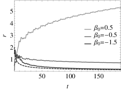
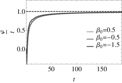
Figure 3. The evolution of $r(t)$ and $\varphi(t)/t$ for solutions to system (55) with $h=2$, $p=3$, $\alpha_{0}=\alpha_{1}=\beta_{1}=\gamma_{0}=\gamma_{1}=s_{2}=1$ and different values of the parameter $\beta_{0}$. The dashed curves correspond to (a) $r(t)\equiv 2t^{-1/2}$, (b) $\varphi(t)/t\equiv 1$.

2. Now, let $h=p=2$. The change of the variable (8) reduces system (55) to the form (9) with

$$\Lambda_{1}(\rho)\equiv 0,\quad\Lambda_{2}(\rho)\equiv\frac{\gamma_{0}+\beta_{0}\rho}{2}.$$

In this case, $n=q=2$, $(n,p)\in\mathcal{Q}_{2}$, and assumption (21) holds with $\rho_{0}=-\gamma_{0}/\beta_{0}$ and $\Lambda_{p}^{\prime}(\rho_{0})=\beta_{0}/2$. It follows from Theorem 6 that if $\beta_{0}<0$, then there exists a stable regime for solutions of system (55) such that $r(t)\sim\varrho_{2}(t)$ and $\varphi(t)\sim t$ as $t\to\infty$, where $\varrho_{2}(t)$ is a polynomially stable solution of the corresponding truncated equation (12) with asymptotics (22). We see that $\varrho_{2}(t)\sim-\gamma_{0}/\beta_{0}$ as $t\to\infty$. It follows from Theorem 7 that this asymptotic regime becomes unstable if $\beta_{0}>0$. If $\beta_{0}=0$ and $\gamma_{0}\neq 0$, then assumption (25) holds. In this case, it follows from Theorem 8 that the solutions of system (55) leave the neighbourhood of zero (see Fig. 4).

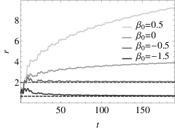
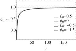
Figure 4. The evolution of $r(t)$ and $\varphi(t)/t$ for solutions to system (55) with $h=p=2$, $\alpha_{0}=\alpha_{1}=\beta_{1}=\gamma_{0}=\gamma_{1}=s_{2}=1$ and different values of the parameter $\beta_{0}$. The dashed curves correspond to (a) $r(t)\equiv 2/3$ and $r(t)\equiv 2$, (b) $\varphi(t)/t\equiv 1$.

3. Let $h=2$ and $p=1$. Then system (55) is transformed to (9) with $\Lambda_{1}(\rho)\equiv\gamma_{0}/2$. In this case, $n=p=1$ and $(n,p)\in\mathcal{Q}_{2}$. If $\gamma_{0}\neq 0$, then assumption (25) holds, and it follows from Theorem 8 that the solutions of system (55) leave the neighbourhood of zero.

4. Finally, let $h=p=3$. In this case, it can easily be checked that system (55) is transformed to (9) with

$$\Lambda_{1}(\rho)\equiv\Lambda_{2}(\rho)=0,\quad\Lambda_{3}(\rho)\equiv\frac{\gamma_{0}+\beta_{0}\rho}{2}.$$

It follows that assumption (11) holds with $n=3>q$, and $(n,p)\in\mathcal{Q}_{3}$. We see that $\Lambda_{3}(\rho)\not\equiv 0$ and $\Lambda_{3}^{\prime}(\rho)\equiv\beta_{0}/2$. Hence, assumption (26) holds if $\rho_{0}\neq-\gamma_{0}/\beta_{0}$. Note that Lemma 6 ensures that the corresponding truncated equation (12) has a stable solution $\varrho_{3}(t)\sim\rho_{0}$ if $\beta_{0}<0$. From Theorem 9 it follows that there exists a regime for solutions of system (55) such that $r(t)\approx\varrho_{3}(t)$ and $\varphi(t)\sim t$ as $t\to\infty$ (see Fig. 5). In this case, the dynamics of the perturbed system (55) is similar to the dynamics of the corresponding limiting system.

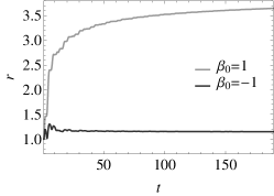
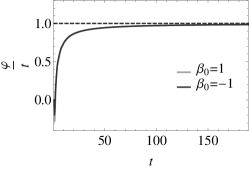
Figure 5. The evolution of $r(t)$ and $\varphi(t)/t$ for solutions to system (55) with $h=p=3$, $\alpha_{0}=\alpha_{1}=\beta_{1}=\gamma_{0}=\gamma_{1}=s_{2}=1$, with the same initial data and different values of the parameter $\beta_{0}$. The dashed curve corresponds to $\varphi(t)/t\equiv 1$.

7.2. Example 2

Consider a system in the Cartesian coordinates

(56) $$\frac{dx}{dt}=y,\quad\frac{dy}{dt}=-\sin x+G(x,y,S(t),t),$$

where

$$G(x,y,S,t)\equiv t^{-\frac{n}{q}}G_{1}(x,y,S)+t^{-\frac{n+d}{q}}G_{2}(x,y,S)+t^{-\frac{p}{q}}G_{3}(x,y,S),$$

$$G_{1}(x,y,S)\equiv\alpha(S)x^{2}y,\quad G_{2}(x,y,S)\equiv\beta(S)y,\quad G_{3}(x,y,S)\equiv\frac{\gamma(S)y}{\sqrt{x^{2}+y^{2}}},$$

$$\alpha(S)=\alpha_{0}+\alpha_{1}\sin S,\quad\beta(S)\equiv\beta_{0}+\beta_{1}\sin S,\quad\gamma(S)\equiv\gamma_{0}+\gamma_{1}\sin S,$$

$S(t)\equiv\sqrt{2}t+\log t$, $\alpha_{j},\beta_{j},\gamma_{j}\in\mathbb{R}$, and $n,d,p,q\in\mathbb{Z}_{+}$ such that $n+d<p$.

We see that system (56) describes damped oscillatory perturbations of the pendulum. Let us show that the proposed theory can be applied to this system.

Note that the corresponding limiting system $dx/dt=\partial_{y}H(x,y)$, $dy/dt=-\partial_{x}H(x,y)$ with $H(x,y)\equiv y^{2}/2-\cos x+1$ has a stable equilibrium at the origin. Moreover, the level lines $\{(x,y):H(x,y)=r^{2}/2\}$ for all $0<|r|<2$, lying in the vicinity of the equilibrium, correspond to periodic solutions $x_{0}(t,r)$, $y_{0}(t,r)$ of the limiting system with a period $T(r)=2\pi/w(r)$, where $w(r)=1-r^{2}/16+\mathcal{O}(r^{4})$ as $r\to 0$. Define auxiliary $2\pi$-periodic functions

$$X(\varphi,r)\equiv x_{0}\left(\frac{\varphi}{w(r)},r\right),\quad Y(\varphi,r)\equiv y_{0}\left(\frac{\varphi}{w(r)},r\right).$$

It can easily be checked that

$$w(r)\partial_{\varphi}X(\varphi,r)\equiv Y(\varphi,r),\quad w(r)\partial_{\varphi}Y(\varphi,r)\equiv-\sin\big{(}X(\varphi,r)\big{)},$$

$$H(X(\varphi,r),Y(\varphi,r))\equiv\frac{r^{2}}{2},\quad{\hbox{\rm det}}\frac{\partial(X,Y)}{\partial(\varphi,r)}\equiv\begin{vmatrix}\partial_{\varphi}X&\partial_{\varphi}Y\\ \partial_{r}X&\partial_{r}Y\end{vmatrix}\equiv\frac{r}{w(r)}.$$

Therefore, system (56) in the variables $(r,\varphi)$ takes the form (1) with $\omega(r)\equiv w(r)$,

$$f(r,\varphi,S,t)\equiv r^{-1}Y(\varphi,r)G(X(\varphi,r),Y(\varphi,r),S,t),$$

$$g(r,\varphi,S,t)\equiv-w(r)\partial_{r}X(\varphi,r)G(X(\varphi,r),Y(\varphi,r),S,t).$$

It can easily be checked that these functions satisfy (3):

$$f(r,\varphi,S,t)\equiv t^{-\frac{n}{q}}f_{1}(r,\varphi,S)+t^{-\frac{n+d}{q}}f_{2}(r,\varphi,S)+t^{-\frac{p}{q}}f_{3}(r,\varphi,S),$$

$$g(r,\varphi,S,t)\equiv t^{-\frac{n}{q}}g_{1}(r,\varphi,S)+t^{-\frac{n+d}{q}}g_{2}(r,\varphi,S)+t^{-\frac{p}{q}}g_{3}(r,\varphi,S),$$

where

$$f_{k}(r,\varphi,S)\equiv r^{-1}Y(\varphi,r)G_{k}(X(\varphi,r),Y(\varphi,r),S),$$

$$g_{k}(r,\varphi,S)\equiv w(r)\partial_{r}X(\varphi,r)G_{k}(X(\varphi,r),Y(\varphi,r),S).$$

Since $X(\varphi,r)=r\cos\varphi+\mathcal{O}(r^{3})$, $Y(\varphi,r)=-r\sin\varphi+\mathcal{O}(r^{3})$ as $r\to 0$, we see that assumption (4) holds with $f_{p,0,0}(0)=\gamma_{0}/2$. Moreover, $S(t)$ has the form (5) with $s_{0}=\sqrt{2}$, $s_{1}=\dots=s_{q-1}=0$, $s_{q}=1$, and assumption (6) holds.

Let $n=d=1$ and $p=q=3$. Then the change of the variable described in Theorem 1 and constructed in Section 3 transforms the system into (9) with

$$\Lambda_{1}(\rho)\equiv\langle f_{1}(\rho,\varphi,S)\rangle_{\varphi,S}=\frac{\alpha_{0}\rho^{3}}{8}(1+\mathcal{O}(|\rho|)),$$

$$\Lambda_{2}(\rho)\equiv\langle f_{2}(\rho,\varphi,S)-\mathcal{R}_{2}(\rho,\varphi,S)\rangle_{\varphi,S}=\frac{\beta_{0}\rho}{2}(1+\mathcal{O}(|\rho|)),$$

$$\Lambda_{3}(\rho)\equiv\langle f_{3}(\rho,\varphi,S)-\mathcal{R}_{3}(\rho,\varphi,S)\rangle_{\varphi,S}=\frac{\gamma_{0}}{2}+\mathcal{O}(|\rho|)$$

as $\rho\to 0$. In this case, $(n+d,q)\in\mathcal{Q}_{3}$, $\mu_{p}=\gamma_{0}/2$ and assumption (18) holds with $m=3$, $\lambda_{n,m}=\alpha_{0}/8$, $\lambda_{n+d}=\beta_{0}/2$. Hence, $m_{\ast}=2$, $\vartheta_{m}=1/6$ and $\mathcal{P}(z)\equiv z(\alpha_{0}z^{2}+4\beta_{0})/8$. If $\alpha_{0}<0$ and $\beta_{0}>0$, then there exists $z_{m}=\sqrt{-4\beta_{0}/\alpha_{0}}$ such that assumption (19) holds with $\mathcal{P}(z_{m})=0$ and $\mathcal{P}^{\prime}(z_{m})=\alpha_{0}z_{m}^{2}/4<0$. It follows from Theorem 5 that there exists a stable regime for solutions of the system with $r(t)\approx\varrho_{m}(t)$ and $\varphi(t)\sim t$, where $\varrho_{m}(t)$ is a solution of the corresponding truncated equation (12) with asymptotics (20). In particular, $\varrho_{m}(t)\sim t^{-1/6}\sqrt{-4\beta_{0}/\alpha_{0}}$ as $t\to\infty$. Returning to the variables $(x,y)$, we obtain $H(x(t),y(t))\approx t^{-1/3}(-2\beta_{0}/\alpha_{0})$ (see Fig. 6).

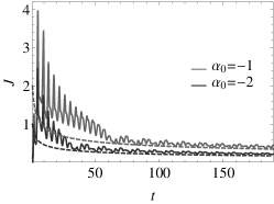
Figure 6. The evolution of $J(t)\equiv H(x(t),y(t))$ for solutions to system (56) with $n=d=1$, $p=q=3$, $\alpha_{1}=\beta_{0}=\beta_{1}=\gamma_{0}=\gamma_{1}=1$ and different values of the parameter $\alpha_{0}$. The dashed curves correspond to $J(t)\equiv 2t^{-1/3}$ and $J(t)\equiv t^{-1/3}$.

8. Conclusion

Thus, possible long-terms asymptotic regimes of solutions to nonlinear oscillatory systems with damped non-resonant perturbations that do not vanish at the equilibrium have been described. We have shown that, depending on the properties of the perturbations, the asymptotically autonomous system can behave like the corresponding limiting system in the vicinity of the equilibrium. Moreover, new stable regimes associated with the solutions of the corresponding truncated systems may appear. For example, there may be exponentially or polynomially stable solutions with amplitude tending to zero or a non-zero constant. It have been also shown that non-resonant perturbations can lead to instability when the perturbed trajectories leave the neighbourhood of the equilibrium. The results obtained show, in particular, that damped perturbations can be used to control the dynamics of nonlinear oscillatory systems.

Note that resonant perturbations and higher-dimensional systems have not been considered in this paper. In this case, the proposed theory cannot be applied directly due to the problem of small denominators. These cases deserve special attention and will be discussed elsewhere.

References

- [1] A. D. Bruno, I. V. Goryuchkina, Boutroux asymptotic forms of solutions to Painlevé equations and power geometry, Doklady Math., 78 (2008), 681–685.
- [2] C. Castillo-Chávez, H.R. Thieme, Asymptotically autonomous epidemic models. In: O. Arino, D. Axelrod, M. Kimmel, M. Langlais (Eds.), Mathematical Population Dynamics: Analysis of Heterogenity, Theory of Epidemics, vol. 1, Wuertz, 1995, p. 33–50.
- [3] O. Sultanov, Stability and asymptotic analysis of the autoresonant capture in oscillating systems with combined excitation, SIAM J. Appl. Math., 78 (2018), 3103–3118.
- [4] D. Scarcella, Weakly asymptotically quasiperiodic solutions for time-dependent Hamiltonians with a view to celestial mechanics, 2022, arXiv: 2211.06768.
- [5] V. V. Kozlov, S. D. Furta, Asymptotic Solutions of Strongly Nonlinear Systems of Differential Equations, Springer, New York, 2013.
- [6] X. Pan, Stability of smooth solutions for the compressible Euler equations with time-dependent damping and one-side physical vacuum, Journal of Differential Equations, 278 (2021), 146–188.
- [7] J. Dong, J. Li, Analytical solutions to the compressible Euler equations with time-dependent damping and free boundaries, J. Math. Phys., 63 (2022), 101502.
- [8] J. A. Langa, J. C. Robinson, A. Suárez, Stability, instability and bifurcation phenomena in nonautonomous differential equations, Nonlinearity, 15 (2002), 887–903.
- [9] P. E. Kloeden, S. Siegmund, Bifurcations and continuous transitions of attractors in autonomous and nonautonomous systems, Internat. J. Bifur. Chaos., 15 (2005), 743–762.
- [10] M. Rasmussen, Bifurcations of asymptotically autonomous differential equations, Set-Valued Anal., 16 (2008), 821–849.
- [11] L. Markus, Asymptotically autonomous differential systems. In: S. Lefschetz (ed.), Contributions to the theory of nonlinear oscillations III, Ann. Math. Stud., vol. 36, pp. 17–29, Princeton University Press, Princeton, 1956.
- [12] L. D. Pustyl’nikov, Stable and oscillating motions in nonautonomous dynamical systems. A generalization of C. L. Siegel’s theorem to the nonautonomous case, Math. USSR-Sbornik, 23 (1974), 382–404.
- [13] H. Thieme, Asymptotically autonomous differential equations in the plane, Rocky Mountain J. Math., 24 (1994), 351–380.
- [14] O. A. Sultanov, Damped perturbations of systems with center-saddle bifurcation, Internat. J. Bifur. Chaos., 31 (2021), 2150137.
- [15] W. A. Harris and D. A. Lutz, Asymptotic integration of adiabatic oscillators, J. Math. Anal. Appl., 51 (1975), 76–93.
- [16] M. Pinto, Asymptotic integration of Second-Order Linear Differential Equations, J. Math. Anal. Appl., 111 (1985), 388–406.
- [17] P. N. Nesterov , Averaging method in the asymptotic integration problem for systems with oscillatory-decreasing coefficients, Differ. Equ. 43 (2007), 745–756.
- [18] V. Burd, P. Nesterov, Parametric resonance in adiabatic oscillators, Results. Math., 58 (2010), 1–15.
- [19] O. A. Sultanov, Bifurcations in asymptotically autonomous Hamiltonian systems under oscillatory perturbations, Discrete & Continuous Dynamical Systems, 41 (2021), 5943–5978.
- [20] O. A. Sultanov, Decaying oscillatory perturbations of Hamiltonian systems in the plane, Journal of Mathematical Sciences, 257 (2021), 705–719.
- [21] J. D. Dollard, C. N. Friedman, Existence of the Møller wave operators for , Annals of Physics, 111 (1978), 251–266.
- [22] M. Ben-Artzi, A. Devinatz, Spectral and scattering theory for the adiabatic oscillator and related potentials, J. Math. Phys., 20 (1979), 594–607.
- [23] O. A. Sultanov, Capture into resonance in nonlinear oscillatory systems with decaying perturbations, Journal of Mathematical Sciences, 262 (2022), 374–389.
- [24] O. A. Sultanov, Resonances in asymptotically autonomous systems with a decaying chirped-frequency excitation, Discrete and Continuous Dynamical Systems — B, 28 (2023), 1719–1749.
- [25] W. Wasow, Asymptotic Expansions for Ordinary Differential Equations, John Wiley and Sons, Inc., New York, 1966.
- [26] N. N. Bogolubov, Yu. A. Mitropolsky, Asymptotic Methods in Theory of Non-linear Oscillations, Gordon and Breach, New York, 1961.
- [27] A. I. Neishtadt, The separation of motions in systems with rapidly rotating phase, J. Appl. Math. Mech., 48 (1984), 133–139.
- [28] V. I. Arnold, V. V. Kozlov, A. I. Neishtadt, Mathematical Aspects of Classical and Celestial Mechanics, Springer, Berlin, 2006.
- [29] L. A. Kalyakin, Lyapunov functions in theorems of justification of asymptotics, Mat. Notes, 98 (2015), 752–764.