Regular access to constantly renewed online content favors radicalization of opinions

Abstract

Worry over polarization has grown alongside the digital information consumption revolution. Where most scientific work considered user-generated and user-disseminated (i.e., Web 2.0) content as the culprit, the potential of purely increased access to information (or Web 1.0) has been largely overlooked. Here, we suggest that the shift to Web 1.0 alone could include a powerful mechanism of belief extremization. We study an empirically calibrated persuasive argument model with confirmation bias. We compare an offline setting—in which a limited number of arguments is broadcast by traditional media—with an online setting—in which the agent can choose to watch contents within a very wide set of possibilities. In both cases, we assume that positive and negative arguments are balanced. The simulations show that the online setting leads to significantly more extreme opinions and amplifies initial prejudice.

1 Introduction

Political polarization—whether affective, ideological or network polarization—seems to be growing in many countries over the last decades. For instance, the divide between liberals and conservatives in the U.S. or between globalists and populists in Europe appears deeper today than ever before. As a result, we have seen massive violent protests and increased institutional instability. It is thus important to better understand the causes of polarization.

It is often suggested that increased access to online media that took place during the same period could have contributed polarization. The popularity of the Internet has revolutionized the way we consume and share information. Web 1.0 (i.e., cognition-oriented) technologies have liberated access to information, Web 2.0 (communication-oriented) has democratized information sharing and Web 3.0 (cooperation-oriented) have made it possible to more easily coordinate actions [16]. While all three technological waves have impacted opinion formation processes, the majority of the scientific work linking political polarization to the popularity of the internet has focused on Web 2.0 aspects of, mainly, online social media. In particular, on communication in digital “echo chambers” created by algorithmic “filter bubbles” in which large groups of users sharing similar views about a topic reinforce each other in their views [4, 22]. Moreover, the unprecedented competition for attracting the attention of users also favors extreme and negative content, particularly in messages of limited size (like on Twitter), which may also lead to opinion radicalization and entrenchment, without algorithmic selection.

In this paper, we focus on the Web 1.0 aspects of the information revolution. How did regular access to a wide diversity of constantly renewed contents about any topic affect the opinion formation of individual users? Before the emergence of online media, the means to access news was limited to a small set of newspapers or TV channels, that strongly frame debates. The situation changed radically, as the new media offer an almost infinite variety of comments and viewpoints, constantly changing, among which the users navigate.

In order to address how Web 1.0 affects individual opinions, we consider a recent, empirically-grounded model of opinion dynamics under biased processing [8]. Here, an individual’s opinion is the aggregate of attitudes towards a series of known arguments, in line with Persuasive Argument Theory (PAT) [31]. Typically, computational models of social influence consider the state variable to be the opinion of the agents, and this opinion evolves according to assumed rules during interactions [14]. In contrast, in the model considered in this paper, the state of the agent is defined by its beliefs about different arguments and these beliefs in association with the valence of the related arguments (for or against a topic) define the agent’s opinion [6, 28].

The assumption that individuals engage in biased processing is by no means a stretch as it is well-grounded in literature on confirmation bias [32]. Confirmation bias predicts that given the same argument, two individuals may react differently as a function of their currently held belief. Specifically, arguments that are closer to the currently held belief are considered stronger than those farther away [21, 35]. Despite the prominence of confirmation bias, only very few opinion dynamics models take it into account [8, 10, 14, 36], the bounded confidence family of models [11, 19] being a prominent exception.

Comparing the mechanisms of biased processing between online and offline contexts is particularly interesting for two main reasons. First, it might be the case that biased processing and the availability of more information due to Web 1.0 alone is enough to explain differences in polarization between online and offline contexts with the calibrated model from Banisch and Shannon [8]. Here, we investigate whether this is the case by looking at how opinions are affected as a function of low (offline) or high (online) availability of information. Second, many contributions in psychology from recent years have shown how consumption of information online, in particular on online social media, affects biased processing. There is ample evidence showing that online, confirmation bias for the selection and processing of information is strong [25] and may be stronger online than offline [33]. Some argue that motivated reasoning—here referring to explicitly seeking out information that confirms currently held beliefs [26]—could account for this effect [29]. But when it comes to actual attitude change (as opposed to mere selection of information), it appears that this effect obtains mostly because people tend to respond differently when overwhelmed with information, rather than through motivated reasoning [34]. Information overload thus strengthens individual tendencies to process new information in light of what they know, rather than in relation to the quality of this information [18]. This implies that online, people might not only be confronted with more options to find information that suits their beliefs best, but that their way to consider content is modified by the abundance of signals. Here, we investigate the effect of strength of confirmation bias in both the online and offline context.

In what follows, we define stylized situations that respectively correspond to offline and online information landscapes and we compare the results obtained in computer simulations with the model for different levels of confirmation biases in these two different contexts. Our work speaks to seminal experimental work on confirmation bias [27] which has shown that individuals may “draw undue support for their initial positions from mixed or random empirical findings” (p. 2098). The model leads to testable hypotheses about how individuals are expected to change their opinion in different information settings characterized more (online) or less (offline) information diversity.

2 Biased dynamics of argument endorsement

2.1 The general model

In this simple setting, we consider a single agent that has a prior belief $\alpha\in[-1,1]$ about a given topic. The agent has access to $N_{a}$ arguments about the topic. We assume that each argument $i\in\{1,...,N_{a}\}$ is either in favor of (then $v_{i}=1$) or against the topic (then $v_{i}=-1$).

The state of the agent is characterized by two vectors:

• The knowledge vector $(k_{i})_{i\in\{1,...,N_{a}\}}$. For each argument $i$, if the agent knows the argument $i$, then $k_{i}=1$ otherwise, $k_{i}=0$.

• The belief vector $(b_{i})_{i\in\{1,...,N_{a}\}}$. For each argument $i$, if the agent believes the argument $i$, then $b_{i}=1$ otherwise, $b_{i}=0$. If the agent does not know the argument, then $b_{i}=0$.

Then, the balance of beliefs $\overline{b}$ of the agent about the considered topic is the sum of its prior belief and the beliefs multiplied by the values of the arguments, for the arguments known by the agent:

$$\overline{b}=\alpha+\sum_{i=1}^{N_{a}}b_{i}v_{i}.$$ (1)

The dynamics rules the determination of beliefs about new arguments. Let $\overline{b}(t)$, $k_{i}(t)$ and $b_{i}(t)$ be respectively the balance of beliefs, the knowledge and the beliefs of the agent at time $t$. Assume that at time $t+1$ the agent accesses to $2q\leq N_{a}$ arguments $j_{1},..,j_{2q}$. Then, for $j\in\{j_{1},...,j_{2q}\}$:

• If $k_{j}(t)=1$, the agent knows the argument and does not change its knowledge or belief. Thus $k_{j}(t+1)=k_{j}(t)$ and $b_{j}(t+1)=b_{j}(t)$.

• If $k_{j}(t)=0$:

  • The agent acquires the knowledge about the argument: $k_{j}(t+1)=1$.

  • The agent determines its belief about the argument. $b_{j}(t+1)=1$ with probability :

    $$P(b_{j}(t+1)=1)=\frac{1}{1+\exp(-\beta\overline{b}(t)v_{j})}.$$ (2)

    Otherwise, $b_{j}(t+1)=0$. The probability to believe the item depends thus on parameter $\alpha$ and $\beta$. Parameter $\alpha$ is a prior belief of the agent about the issue. Parameter $\beta$ rules the confirmation bias in the beliefs. The higher is $\beta$ the higher the tendency to believe items in the direction of the current balance of beliefs $\overline{b}$.

Moreover, for $i\notin\{j_{1},..,j_{2q}\}$ $k_{i}(t+1)=k_{i}(t)$, $b_{i}(t+1)=b_{i}(t)$. Finally, the attitude of the agent about the topic is updated:

$$\overline{b}(t+1)=\alpha+\sum_{i=1}^{N_{a}}b_{i}(t+1)v_{i}.$$ (3)

We also define the attitude $a(t)\in[-1,1]$ of the agent, as follows :

$$a(t)=2\left(\frac{1}{1+\exp(-\beta\overline{b}(t)})-\frac{1}{2}\right).$$ (4)

The attitude aims at quantifying how the agent is favorable or unfavorable to the issue at stake. In the model this attitude is expressed by the propensity of the agent to accept arguments from one side or the other. When the attitude is positive, its value is the probability that the agent believes a positive argument. When it is negative, its opposite is the probability that the agent believes a negative argument. When the attitude is close to 1 or -1, this corresponds to an extreme attitude, as the agent is completely close to the opposite side and systematically accepts any argument on their own side. As a result, for the same balance of beliefs, two agents having different confirmation biases (ruled by parameter $\beta$) have different attitudes towards the issue.

2.2 Offline setting

The typical situation that we aim to represent here is an individual consuming TV or newspaper reports in which the pro and contra arguments about the topic are balanced, but limited. In this offline setting, we assume that, at each time step, the agent is exposed to $2q\leq N_{a}$ arguments $j_{1},..,j_{2q}$ such that the overall valence of the argument is neutral:

$$\sum_{i=1}^{2q}v_{j_{i}}=0$$ (5)

Hence, we have $q$ arguments of each sign.

Once the agent knows all the arguments, its attitude remains fixed. Let $T$ be the time when this situation is reached. In the agent simulations, we start with all knowledge $(k_{i})$ is equal to 0. We run the model for a number of steps $T$ and compute the final distribution of opinions for different values of the total number of arguments $N_{a}$ and the number exposed $2q$ at each time step, .

We do not have to repeat computer simulations in order to evaluate the average results, as the model can be represented as a Markov chain ruling the probabilities of being in states defined by four integer values. Here, a state of the Markov chain is indeed defined by the vector $(K_{+},B_{+},K_{-},B_{-})$ of, respectively, the number of known positive arguments, the number of believed positive arguments, the number of known negative arguments, and the number of believed negative arguments.

$$K_{+} =\sum_{i=1}^{n_{a}}k_{i},\mbox{ }K_{-}=\sum_{i=n_{a}+1}^{N_{a}}k_{i},$$ (6)

$$B_{+} =\sum_{i=1}^{n_{a}}b_{i},\mbox{ }B_{-}=\sum_{i=n_{a}+1}^{N_{a}}b_{i}.$$ (7)

As the number of believed arguments is lower or equal to the number of known arguments, the total number of states is $N_{S}=\frac{1}{4}(n_{a}+1)^{2}(n_{a}+2)^{2}$.

Considering an agent in the state $S=(K_{+},B_{+},K_{-},B_{-})$, we can express the probability $P(S,S^{\prime})$ that the agent goes to the state $S^{\prime}=(K^{\prime}_{+},B^{\prime}_{+},K^{\prime}_{-},B^{\prime}_{-})$ after being exposed to a random neutral set of $q$ arguments. Starting with a probability 1 of being in the state $S_{0}=(0,0,0,0)$, we can evolve the probabilities of the different states after each step. In this case, as the number of arguments is limited, when the number of steps increase indefinitely, the model converges to a fixed probability distribution. Appendix 0.A.1 provides the details of this model.

2.3 Online setting

In the online setting, agents choose the arguments among a much wider set of signals than in the offline case. Again, we assume that the platform proposes a balanced set of pro and contra arguments.

Consider an agent who selects to consider $2q$ arguments about the topic of interest at each point in time. The choice of the agent is based on the valence (pro or against the considered topic) of the signals. We assume that the selection of arguments to engage with by the agent is biased—which is in line with previous empirical work [3, 29]—governed by $\gamma$. It can be understood as a parameter that governs a first confirmation bias or possibly the degree of motivated reasoning agents engage in [26]. The probability of $c(t,j)$, that the agent chooses to watch content $j$ of valence $v_{j}$ at time $t$, is:

$$P(c(t,j))=\frac{1}{1+\exp(-\gamma\overline{b}(t)v_{j})}.$$ (8)

After choosing what content to engage with, the agent updates its beliefs with the same rules as before. In this case, the agent’s opinion potentially changes all the time, as the agent always considers new arguments. Therefore, we set a time horizon $T$ after which we stop the simulation.

The main difference with the offline setting is that the agent gets more opportunities to choose the content it wants to engage with, and its initial choice is itself subject to confirmation bias. We will consider in particular the case of users who are careful to balance their selection of news (i.e. for whom $\gamma=0$) in order to clearly distinguish between the effects of selection and belief bias.

We can actually represent the state of the agent by the balance of its beliefs minus the prior belief: $\overline{b}-\alpha=B_{+}+B_{-}$. For a time horizon $T$, the state $S$ is an integer in : $\{-2qT,2qT\}$. For any state in $\{-2q(T-1),2q(T-1)\}$, we can compute the transition probabilities to all the states in $\{-2qT,2qT\}$. Then, starting with the system being the state $S=0$ with probability 1, we can compute the probability distribution over all the states at any step $t<=T$. A detailed description of the Markov Chain can be found in Appendix 0.A.2.

3 Simulation results

3.1 Increased extremism in the online setting

3.1.1 Indicator.

The indicator of extremism $E$, is defined at $t$ on the probability distribution $\mu_{t}(\overline{b})$ of the agent holding balance of beliefs $\overline{b}\in\{-B,...B\}$ as the average of the absolute value of the attitude $a(\overline{b})$ (see Eq. 4):

$$E=\sum_{b=-B}^{B}\mu_{t}(\overline{b})\left|a(\overline{b})\right|,$$ (9)

Indeed, if this indicator is close to 1, ti means that the agent’s attitude is very likely to be 1 or -1, in which case the agent accepts all arguments from their side and discards any argument from the opposite side, which fits the usual view of an extreme behaviour.

3.1.2 Examples of comparisons between online and offline settings.

Figure 1 provides examples of comparison of the evolution of normalized opinions between offline and online settings. In these examples, the number of considered arguments at each iteration is 4 in both cases. In the offline setting, two arguments of each sign are chosen at random at each iteration. In the online setting, the agent chooses 4 arguments at random, with no selection bias $\gamma=0$. In the offline model, the total number of arguments is $N_{a}=12$. In the online, the number of arguments increases of 4 at each iteration, as they are assumed new. The bias in the choice of the arguments to consider is $\gamma=0$.

In these examples, polarization is much stronger in the online setting. This is reflected by the extremism indicator which is lower than 0.5 in the offline examples and higher than 0.7 in the online examples.

Figure 2 shows the evolution of the logarithm of the distribution of balance of beliefs for the same examples as Figure 1. Indeed, after a few iterations, especially in the online case, without the logarithm, the values of the distribution are very small and difficult to distinguish. These figures show that, in the online case, the agent has a high probability to reach balances of beliefs which are higher than 20 or lower than -20, whereas in the online case, the opinions are most likely between -3 and +3. In the online case, the distribution is steadily enlarged at each iteration, which increases the likelihood of extremism. As the number of arguments is fixed in the offline case, the tendency to become more extreme comes only from the discovery of unknown arguments.

		Offline	Online
$\beta=0.25$	Attitude
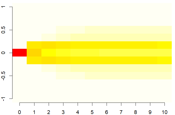
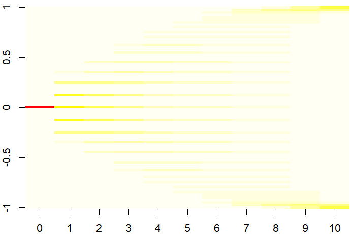
		Iterations $t$	Iterations $t$
		$E(10)=0.21$	$E(10)=0.73$
$\beta=0.5$	Attitude
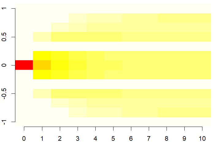
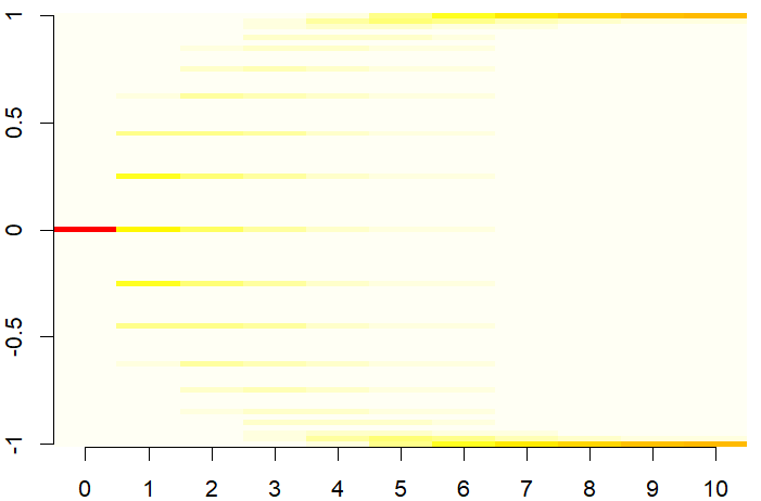
		Iterations $t$	Iterations $t$
		$E(10)=0.46$	$E(10)=0.96$

Figure 1: Evolution of the distribution of attitude in Online and offline Markov models. In both models, the number of arguments considered at each iteration is $2q=4$ and the initial bias $\alpha=0$. The total number of arguments in the offline model is $N_{a}=12$. In the online model, the choice bias is $\gamma=0$. In each case, the extremism indicator $E$ is computed at the last iteration.

		Offline	Online
$\beta=0.25$	Balance of beliefs
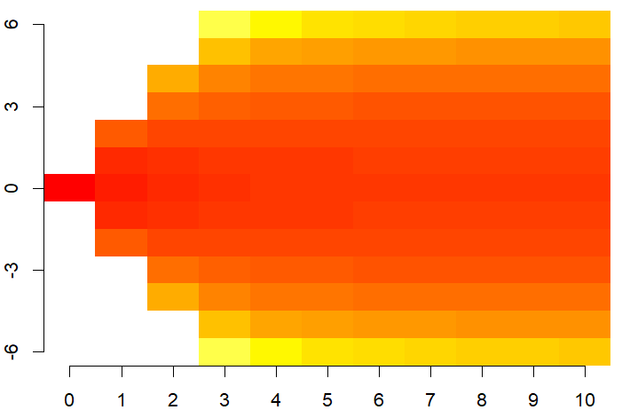
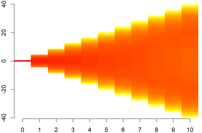
$\beta=0.5$	Balance of beliefs
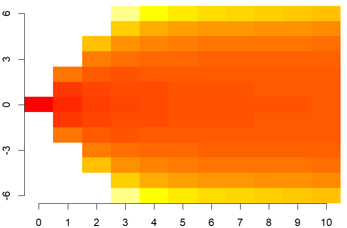
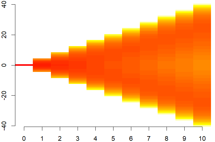
		Iterations	Iterations

Figure 2: Evolution of the logarithm of the distribution of the balance of beliefs $\overline{b}(t)$ in Online and offline Markov models. The parameters are the same as on Figure 1. In both models, the number of arguments considered at each iteration is $2q=4$ and the initial bias $\alpha=0$. The total number of arguments in the offline model is $N_{a}=12$. In the online model, the choice bias is $\gamma=0$. In each case, the extremism indicator $E$ is computed at the last iteration.

3.1.3 Effects of different parameters on extremism.

Figure 3 shows how the extremism indicator evolves with the number of iterations $t$, for different values of the belief confirmation bias parameter $\beta$. For the considered values of the parameters, in the offline case, extremism remains almost constant after 4 or 5 iterations. On the contrary, in the online case, extremism continues to strongly increase until the last iterations for all values of $\beta$. This increase gets smaller when the extremism reaches values that are close to 1, like for $\beta=0.5$.

This constant increase of the extremism in the online setting can be explained by the shape of the distribution of balances of beliefs over time as shown on Figure 2, on the left panels. Indeed, at each iteration, there is a high probability to get a stronger balance of beliefs by adding new positive or negative beliefs. In the offline setting, this increase is constrained by the limited number of items.

Figure 4 shows the effect of $\gamma$, the bias in the choice of the items (online setting), on the evolution of the extremism for different values of the bias in the belief of items $\beta$. All the other parameters being the same as on Figure 1. The result shows a substantial increase of the extremism for $\gamma=0.2$ and even more for $\gamma=0.4$.

The effect of parameter $\gamma$ is actually very similar to the effect of a selection algorithm that could be implemented by the platform. It plays the role of a filter prior to a more careful attention devoted to the item.

	Offline		Online $\gamma=0$
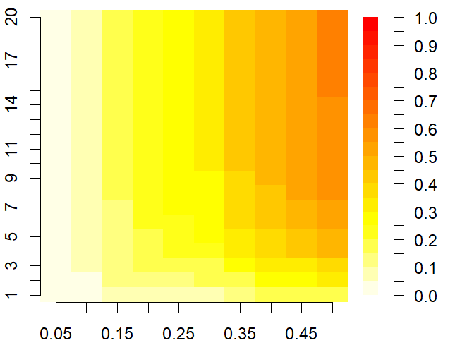
Iterations $t$		Iterations $t$
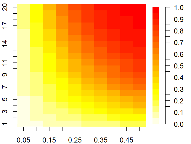
	$\beta$		$\beta$

Figure 3: Extremism indicator during iterations. Left panel: offline. Right panel: Online. The parameters are the same as on Figure 1.

	Online $\gamma=0.2$		Online $\gamma=0.4$
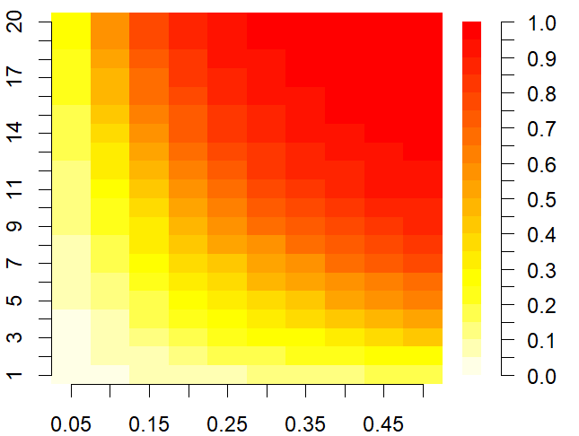
Iterations $t$		Iterations $t$
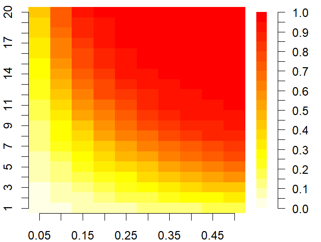
	$\beta$		$\beta$

Figure 4: Extremism indicator during iterations for online setting. Effect of the bias in item choice parameter $\gamma$. The other parameters are the same as on Figure 1.

3.2 Amplification of prejudice in online setting

3.2.1 Indicator.

Let $\mu_{t}(\overline{b})$ be the probability distribution of the balance of beliefs $\overline{b}$, varying between $-B+\alpha$ and $B+\alpha$ at iteration $t$.

The prejudice $P(t)$ is defined as the average of the attitude:

$$P(t)=\sum_{b=-B+\alpha}^{B+\alpha}a(\overline{b})\mu_{t}(\overline{b}),$$ (10)

where $a(\overline{b})$ is the attitude associated with the balance of beliefs as specified by equation 4. The value of this indicator is in $[-1,1]$ and expresses the average tendency to believe positive or negative items. It is 0 when the distribution is symmetric, that is, when the probability to believe negative or positive items are the same (as it is always the case when the initial opinion $\alpha=0$). It is positive if the agent has a higher probability to believe positive than negative items, it is negative in the opposite case. Note that, at $t=0$, $P(0)$ is simply the attitude at $t=0$ because the distribution is all concentrated (Dirac distribution) at value $\alpha$.

In the following, we measure the relative increase $I_{P}(t)$ of the prejudice over time which is:

$$I_{P}(t)=1-\frac{P(0)}{P(t)}$$ (11)

In other words, $I_{P}(t)$ express to what extent the prejudice is amplified over time.

3.2.2 Examples.

Figure 5 shows examples of model runs with an initial bias $\alpha=0.5$. In this case the distribution is asymmetric. In both cases the initial prejudice $P(0)=0.05$. However, at $t=10$, we have $P(10)=0.08$ for the offline setting and $P(10)=0.18$ for the online setting. This example suggests that the initial prejudice tends to increase more with the interactions in the online setting.

		Offline	Online
$\beta=0.25$	Normalized opinions
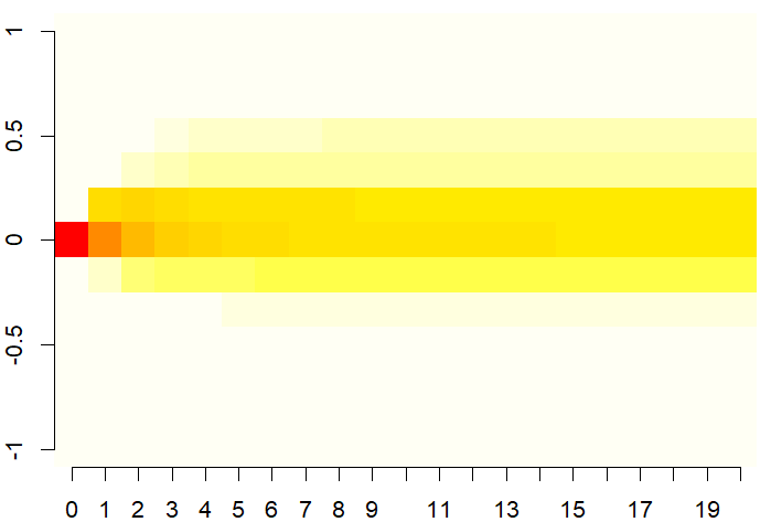
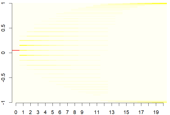
		Iterations $t$	Iterations $t$
		$P(10)=0.08$	$P(10)=0.18$

Figure 5: Initial bias $\alpha=0.5$. Evolution of the distribution of normalized opinions in online and offline Markov models. In both models, the bias on item belief is $\beta=0.2$. In each case, the prejudice indicator $P$ is computed at the last time step.

3.2.3 Systematic simulations.

Figure 6 shows the relative increase of prejudice $I_{P}(t)$ for different values of $\beta$ and for a prior belief $\alpha=0.5$. In the online setting, the figure shows the results for 3 values of the bias in the choice of the items $\gamma\in\{0,0.2,0.4\}$.

When $\gamma=0$, the relative increase of prejudice is higher in the online than in the offline setting for $0.1\leq\beta\leq 0.25$. However, for $\beta>0.25$, the final relative increase of prejudice is higher in the offline setting.

Overall, the relative amplification of the prejudice is even higher when the bias on belief $\beta$ is small (for $\gamma=0.2$, and even more for $\gamma=0.4$), while the opposite is true in the offline case. Moreover, the amplification of the prejudice is higher online than offline for all values of $\beta$, and the increase takes place more rapidly (after 6 or 7 iterations).

	Offline		Online $\gamma=0$
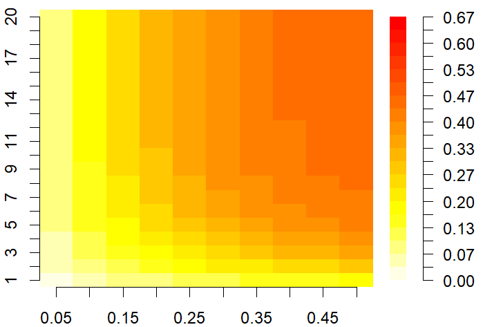
Iterations $t$		Iterations $t$
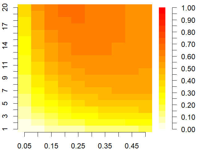
	$\beta$		$\beta$
	Online $\gamma=0.2$		Online $\gamma=0.4$
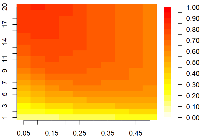
Iterations $t$		Iterations $t$
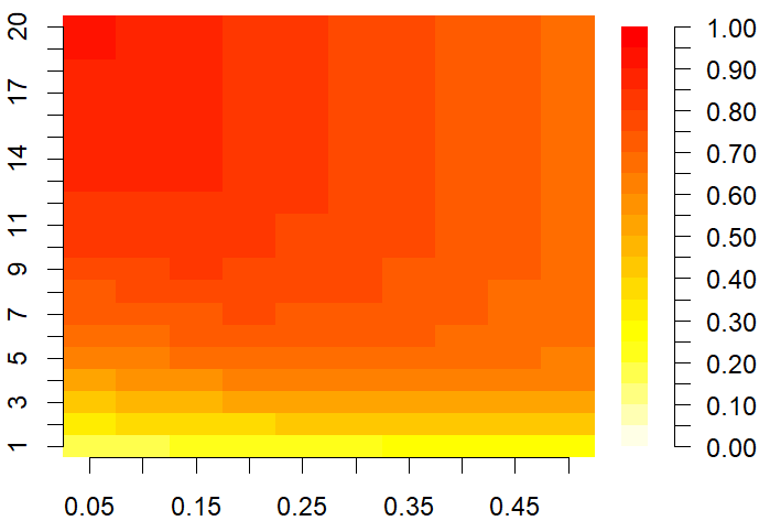
	$\beta$		$\beta$

Figure 6: Relative increase of prejudice $I_{P}(t)=1-\frac{P(0)}{P(t)}$. The non-specified parameters are the same as on Figure 1.

4 Discussion

The Web 1.0 revolution brought regular access to a wide diversity of constantly renewed content about any topic to the billions of people connected to the internet. Our model suggest that this access to online content increases the effect of cognitive biases (i.e., confirmation bias and motivated reasoning) which amplifies bi-polarization, extremization and prejudice. Algorithmically-induced selective exposure (associated with Web 2.0) certainly increases these effects even more, but the role of the almost infinite choice of contents offered by online environments should not be neglected. This point resonates with effects of ‘globalization’ or network size in other modeling traditions [1, 11, 12, 19, 20, 23, 24] and invites to refrain putting the blame of polarization exclusively or even majorly on web personalization [22].

The model introduced in this paper is based on a recent contribution that experimentally calibrated the agents’ influence-response function after exposure to a balanced set of arguments [8]. The approach relies on several assumptions that deserve further investigation, in our view. First, all beliefs are considered dichotomous. The agents either completely believe or completely reject an argument. However, it is often the case that we believe more or less an argument. It would be important to investigate if a model introducing several levels of beliefs would show the same effects. Second, all arguments hold the same weight when the aggregate opinion is constructed. How opinions are precisely constructed from a set of arguments is an open empirical question, but as some motivated reasoning scholars point to the active construction of the same known arguments to reach different conclusions [2, 13, 26], it is likely that there is some form of weighing of arguments involved. Our model showed that different opinions can emerge given the same information, if that information is evaluated based on some biased belief. When weighing gets involved, different opinions can also emerge between agents who believe the same information. Such a model could resonate well with the reality of radically different interpretations accepting the same facts, which we have seen during even the largest of societal challenges such as COVID-19 or in the climate change mitigation debate.

While enriching the model with more complex processes and calibrating those processes to empirical micro and macro-level data could improve our understanding of cognition and information consumption in different contexts, we believe that the main conclusions from this paper are likely to hold up. The discussion framed by traditional media focuses on a limited set of arguments, because they should meet the interest of a wide audience. Introducing very specific points or details introduces a high risk to loose the average reader or spectator. With the freedom to browse on a virtually infinite set of arguments, online information consumers can find large set of items that fit perfectly their specific interest, dig deeper and deeper in their own direction, ultimately forging a robust, likely extreme, opinion.

The work presented here fits into a broader tradition of social simulation models that have tried to tackle the question of globalization from different angles. Our findings resonate with those from the bounded confidence tradition [11, 19] where confirmation bias can produce the empirical macro-patterns observed online [12]. They echo results from nominal opinion models in the tradition of Axelrod [1] with globalization causing fragmentation, not consensus  [24] and online communication creating large cleavages between those who think differently [5, 23]. What is more, they fit the results from the Construct-model tradition [9] that, much like PAT, considers the adoption of facts based on information processing biases [30].

We propose a number of possible avenues for future theoretical and experimental research based on the model discussed here, that stand between this abstract model and the patterns we see at a macro-scale in reality [15]. Theoretically, the addition of information filtering systems can be an interesting extension to the model. Web personalization can be implemented in many ways—for instance, as network-based, popularity-based or cultural distance-based filters—and the choice for a particular filtering procedure may have profound impacts on the dynamics of opinions [22]. One could also imagine to integrate this model with the model from Geschke et al. [17] who considered individual, social and technological filters. In order to capture aspects of the Web 2.0 the model should be enriched by incorporating social networks and social influence components [7, 14]. Networks dictate how information spreads through a population. Both social structure and the way in which communication is structured vary between on and offline contexts and may impact model dynamics [23]. Finally, including multiple opinions that co-evolve [6] could create more complex agent profiles and possibly overcome amplification of initial bias.

The research presented here also resulted in promising directions for experimental research. While this model is built upon empirical work by Banisch and Shannon [8], the previous work did not consider crowded (nor infinte) information environments. What is more, the model here is extended with a selection bias (modeled as $\gamma$ in Eq. 8). An extension of the original experiment [35] could consider the information selection process introduced here and control the amount of information that individuals can choose to engage with. This would allow to empirically calibrate the selection bias $\gamma$ and validate the conjectures of this paper.

The digital revolution has come with many challenges, of which increasing polarization is just one. Theoretical explanations like the one outlined in this paper help to understand the logic of assumed causal links, and point to where the culprits may be. We have shown that we need not assume that polarization arises from advanced Web 2.0 selective exposure, complex social network topologies or heterogenous influence-response functions, but that a cognitive processing suffices to generate extremization. Interpret these findings at your own risk.

Appendix 0.A Appendix: Details of the Markov models

0.A.1 Model with offline interactions

The model includes $N_{a}=2n_{a}$ arguments in total and during $T$ time steps, at each time step, the agent receives information about $q$ positive and $q$ negative arguments, chosen at random among the $N_{a}$ possible arguments.

The different states of the agent are defined by four integers $(k_{p},k_{n},b_{p},b_{n})$, where $k_{p}\in\{0,...,n_{a}\}$ is the number of positive arguments known by the agent, $k_{n}\in\{0,...,n_{a}\}$ is the number of negative arguments known by the agent, $b_{p}\in\{0,...,k_{p}\}$ is the number of positive arguments believed by the agent and $b_{n}\in\{0,...,k_{n}\}$ is the number of negative arguments believed by the agent. Let $\mathcal{S}$ be the total set of these possible states.

Let $\mu_{t}(k_{p},k_{n},b_{p},b_{n})$ be the probability that the agent is in state $(k_{p},k_{n},b_{p},b_{n})$. We assume: $\mu_{0}(0,0,0,0)=1$ and for all the other states, $\mu_{0}(k_{n},k_{p},b_{p},b_{n})=0$.

Then, at each step $t\in\{1,...,T-1\}$, we compute $\mu_{t+1}$ from $\mu_{t}$. This is done as follows:

1. We initialise the difference distribution $\delta(k_{p},k_{n},b_{p},b_{n})=0$, for all $(k_{p},k_{n},b_{p},b_{n})\in\mathcal{S}$.

2. For all states $(k_{p},k_{n},b_{p},b_{n})\in\mathcal{S}$ such that $\mu_{t}(k_{p},k_{n},b_{p},b_{n})>0$:

   1. There are $n_{a}-k_{p}$ unknown positive arguments and $n_{a}-k_{n}$ negative arguments. The maximum of new arguments received is thus $m_{p}=\min(q,n_{a}-k_{p})$ positive and $m_{n}=\min(q,n_{a}-k_{n})$ negative arguments. As the arguments are assumed randomly chosen, the probability that the agent gets a new positive argument is $P_{kp}=\frac{m_{p}}{n_{a}}$ and the probability to get $i_{p}\in\{0,...,m_{p}\}$ new arguments is (Bernoulli formula):

      $$P(k^{\prime}_{p}=k_{p}+i_{p})=\binom{i_{p}}{m_{p}}P_{kp}^{i_{p}}(1-P_{kp})^{m_{p}-i_{p}}.$$ (12)

      Similarly, the probability that the agent gets a new positive argument is $P_{kn}=\frac{m_{n}}{n_{a}}$ and the probability to get $i_{n}\in\{0,...,m_{n}\}$ new arguments is :

      $$P(k^{\prime}_{n}=k_{n}+i_{n})=\binom{i_{n}}{m_{n}}P_{kn}^{i_{n}}(1-P_{kn})^{m_{n}-i_{n}}.$$ (13)

   2. For each new positive argument among $i_{p}$, the probability to believe this argument is:

      $$P_{bp}=\frac{1}{1+\exp(-\beta(b_{p}-b_{n}+\alpha))}.$$ (14)

      Hence, the probability to believe $j_{P}\in\{0,...,i_{p}\}$ positive arguments among the $i_{p}$ new ones is:

      $$P(b^{\prime}_{p}=b_{p}+j_{p})=\binom{j_{p}}{i_{p}}P_{bp}^{j_{p}}(1-P_{bp})^{i_{p}-j_{p}}.$$ (15)

      Similarly, for each new negative argument among $i_{n}$, the probability to believe this argument is:

      $$P_{bn}=\frac{1}{1+\exp(\beta(b_{p}-b_{n}+\alpha))}.$$ (16)

      Hence, the probability to believe $j_{n}\in\{0,...,i_{n}\}$ negative arguments among the $i_{n}$ new ones is:

      $$P(b^{\prime}_{n}=b_{n}+j_{n})=\binom{j_{n}}{i_{n}}P_{bn}^{j_{n}}(1-P_{bn})^{i_{n}-j_{n}}.$$ (17)

   3. For all considered values $i_{p}$, $i_{n}$, $j_{p}$, $j_{n}$, let:

      $$dP=P(k^{\prime}_{n}=k_{n}+i_{n})P(k^{\prime}_{n}=k_{n}+i_{n})P(b^{\prime}_{p}=b_{p}+j_{p})P(b^{\prime}_{n}=b_{n}+j_{n}).$$ (18)

      We update $\delta$ as follows:

      $$\delta(k_{p},k_{n},b_{p},b_{n}) :=\delta(k_{p},k_{n},b_{p},b_{n})-dP$$ (19)

      $$\delta(k_{p}+i_{p},k_{n}+i_{n},b_{p}+j_{p},b_{n}+j_{n}) :=\delta(k_{p}+i_{p},k_{n}+i_{n},b_{p}+j_{p},b_{n}+j_{n})+dP.$$ (20)

3. We update the distribution $\mu_{t}$. For all states:

   $$\mu_{t+1}(k_{p},k_{n},b_{p},b_{n})=\mu_{t}(k_{p},k_{n},b_{p},b_{n})+\delta(k_{p},k_{n},b_{p},b_{n}).$$ (21)

Finally, we compute the distribution of probabilities to have a bias of $2*\left(\frac{1}{1+\exp(-\beta(b+\alpha)}-\frac{1}{2}\right)$, as the sum of $\mu(k_{p},k_{n},b_{p},b_{n})$ for all the couples $(b_{p},b_{n})$ such that $b_{p}-b_{n}=b$.

0.A.2 Model with online interactions

In this case, the set of states is simpler: they correspond to all the possible values of the balance of beliefs $b_{p}-b_{n}$, which are $\mathcal{S}=\{-Tn_{a},...,Tn_{a}\}$, where $T$ is the number of iterations in which the agent consults $2q$ items on the platform.

We define the probability distribution $\mu_{t}(b)$, for $b\in\mathcal{S}$. Initially, $m_{0}(0)=1$, and $\mu_{0}(b)=0$ for $b\neq 0$.

Then, at each step $t\in\{1,...,T-1\}$, we compute $\mu_{t+1}$ from $\mu_{t}$. This is done as follows:

1. We initialise a difference distribution such that $\delta(b)=0$ for all $b\in\mathcal{S}$,

2. for each state $b$ such that $\mu_{t}(b)>0$:

   1. we compute the probability to choose a positive content:

      $$P_{c}=\frac{1}{1+\exp(-\gamma(b+\alpha))}.$$ (22)

      Then, for $c_{p}\in\{0,...,2q\}$ the probability to choose to consult $i_{p}$ positive contents and $q_{a}-c_{p}$ negative contents is:

      $$P_{cp}=\binom{c_{p}}{q_{a}}P_{c}^{c_{p}}(1-P_{c})^{q_{a}-c_{p}}.$$ (23)

   2. Then, the probability to believe $j_{p}\in\{0,...,c_{p}\}$ contents among the chosen $c_{p}$ is:

      $$P(b^{\prime}_{p}=b_{p}+j_{p})=\binom{j_{p}}{c_{p}}P_{b}^{j_{p}}(1-P_{b})^{c_{p}-j_{p}},$$ (24)

      with:

      $$P_{b}=\frac{1}{1+\exp(-\beta(b+\alpha))}.$$ (25)

      Similarly, setting$c_{n}=q_{a}-c_{p}$, the probability to believe $j_{n}\in\{0,...,c_{n}\}$ contents among the chosen $c_{n}$ is:

      $$P(b^{\prime}_{n}=b_{n}+j_{n})=\binom{j_{n}}{c_{n}}P_{n}^{j_{n}}(1-P_{n})^{c_{n}-j_{n}},$$ (26)

      with:

      $$P_{n}=\frac{1}{1+\exp(\beta(b+\alpha))}.$$ (27)

   3. For all the considered $(c_{p},c_{n},i_{p},i_{n})$, let:

      $$dP=\mu(b)P_{cp}P(b^{\prime}_{p}=b_{n}+j_{p})P(b^{\prime}_{n}=b_{n}+j_{n})$$ (28)

      We update the distribution $\delta$ as follows:

      $$\delta(b) :=\delta(b)-dP$$ (29)

      $$\delta(b+j_{p}-j_{n}) :=\delta(b+j_{p}-j_{n})+dP.$$ (30)

3. We update the distribution $\mu_{t}$. For all states:

   $$\mu_{t+1}(b)=\mu_{t}(b)+\delta(b).$$ (31)

Finally, like with the offline model, the distribution of probabilities to have a bias of $2*\left(\frac{1}{1+\exp(-\beta(b+\alpha)}-\frac{1}{2}\right)$, is $\mu(b)$.

References

- [1] Axelrod, R.M.: The dissemination of culture: A model with local convergence and global polarization. Journal of Conflict Resolution 41(2), 203–226 (1997). https://doi.org/10.1177/0022002797041002001, arXiv: 0803973233 ISBN: 0022-0027
- [2] Babcock, L., Loewenstein, G.: Explaining bargaining impasse: the role of self-serving biases. Journal of Economic Perspectives 11(1), 109–126 (1997). https://doi.org/10.1257/jep.11.1.109
- [3] Bakshy, E., Messing, S., Adamic, L.A.: Exposure to ideologically diverse news and opinion on Facebook. Science 348(6239), 1130–1132 (2015). https://doi.org/10.1126/science.aaa1160
- [4] Banisch, S., Gaisbauer, F., Olbrich, E.: Modelling spirals of silence and echo chambers by learning from the feedback of others. Entropy 24(10), 1484 (2022)
- [5] Banisch, S., Olbrich, E.: Opinion polarization by learning from social feedback. The Journal of Mathematical Sociology 43(2), 76–103 (2019)
- [6] Banisch, S., Olbrich, E.: An argument communication model of polarization and ideological alignment. Journal of Artificial Societies and Social Simulation 24(1) (2021)
- [7] Banisch, S., Shamon, H.: Validating argument-based opinion dynamics with survey experiments. arXiv preprint arXiv:2212.10143 (2022)
- [8] Banisch, S., Shannon, H.: Biased processing and opinion polarisation: Experimental refinement of argument communication theory in the context of the energy debate. arXiv preprint arXiv:2212.10117 (2022). https://doi.org/10.48550/arXiv.2212.10117
- [9] Carley, K.: A Theory of Group Stability. American Sociological Review 56(3), 331 (Jun 1991). https://doi.org/10.2307/2096108
- [10] Dandekar, P., Goel, A., Lee, D.T.: Biased assimilation, homophily, and the dynamics of polarization. Proceedings of the National Academy of Sciences 110(15), 5791–5796 (2013)
- [11] Deffuant, G., Weisbuch, F.A.G., Faure, T.: How can extremism prevail? a study based on the relative agreement interaction model. Journal of Artificial Societies and Social Simulation 5(4) (2002)
- [12] Del Vicario, M., Scala, A., Caldarelli, G., Stanley, H.E., Quattrociocchi, W.: Modeling confirmation bias and polarization. Scientific Reports 7(1), 40391 (2017). https://doi.org/10.1038/srep40391
- [13] Epley, N., Gilovich, T.: The mechanics of motivated reasoning. Journal of Economic Perspectives 30(3), 133–140 (Aug 2016). https://doi.org/10.1257/jep.30.3.133
- [14] Flache, A., Maes, M., Feliciani, T., Chattoe-Brown, E., Deffuant, G., Huet, S., Lorenz, J.: Models of social influence: Towards the next frontiers. Journal of Artificial Societies and Social Simulation 20(4) (2017)
- [15] Flache, A., Mäs, M., Keijzer, M.A.: Computational approaches in rigorous sociology: agent-based computational sociology and computational social science. In: Gërxhani, K., De Graaf, N.D., Raub, W. (eds.) Handbook of Sociological Science. Contributions to Rigorous Sociology, pp. 57–72. Edward Elgar Publishing, Cheltenham, UK (2022). https://doi.org/10.4337/9781789909432.00011
- [16] Fuchs, C., Hofkirchner, W., Schafranek, M., Raffl, C., Sandoval, M., Bichler, R.: Theoretical foundations of the web: cognition, communication, and co-operation. towards an understanding of web 1.0, 2.0, 3.0. Future internet 2(1), 41–59 (2010)
- [17] Geschke, D., Lorenz, J., Holtz, P.: The triple-filter bubble: Using agent-based modelling to test a meta-theoretical framework for the emergence of filter bubbles and echo chambers. British Journal of Social Psychology 58(1), 129–149 (Jan 2019). https://doi.org/10.1111/bjso.12286
- [18] Goette, L., Han, H.J., Leung, B.T.K.: Information overload and confirmation bias (2020)
- [19] Hegselmann, R., Krause, U.: Opinion dynamics and bounded confidence: Models, analysis and simulation. Journal of Artificial Societies and Social Simulation 5(3) (2002)
- [20] Jager, W., Amblard, F.: Uniformity, bipolarization and pluriformity captured as generic stylized behavior with an agent-based simulation model of attitude change. Computational & Mathematical Organization Theory volume 10, 295–303 (2005)
- [21] Kappes, A., Harvey, A.H., Lohrenz, T., Montague, P.R., Sharot, T.: Confirmation bias in the utilization of others’ opinion strength. Nature neuroscience 23(1), 130–137 (2020)
- [22] Keijzer, M.A., Mäs, M.: The complex link between filter bubbles and opinion polarization. Data Science 5(2), 139–166 (2022). https://doi.org/10.3233/DS-220054
- [23] Keijzer, M.A., Mäs, M., Flache, A.: Communication in online social networks fosters cultural isolation. Complexity pp. 1–20 (2018). https://doi.org/10.1155/2018/9502872
- [24] Klemm, K., Eguíluz, V.M., Toral, R., San Miguel, M.: Globalization, polarization and cultural drift. Journal of Economic Dynamics and Control 29(1-2), 321–334 (2005). https://doi.org/10.1016/j.jedc.2003.08.005, iSBN: 0165-1889
- [25] Knobloch-Westerwick, S., Mothes, C., Polavin, N.: Confirmation bias, ingroup bias, and negativity bias in selective exposure to political information. Communication Research 47(1), 104–124 (2020)
- [26] Kunda, Z.: The case for motivated reasoning. Psychological Bulletin 108(3), 480–498 (Nov 1990). https://doi.org/10.1037/0033-2909.108.3.480
- [27] Lord, C.G., Ross, L., Lepper, M.R.: Biased assimilation and attitude polarization: The effects of prior theories on subsequently considered evidence. Journal of personality and social psychology 37(11), 2098 (1979)
- [28] Mäs, M., Flache, A.: Differentiation without distancing. explaining bi-polarization of opinions without negative influence. PLOS-One 8(11) (2013)
- [29] Van der Meer, T.G., Hameleers, M., Kroon, A.C.: Crafting our own biased media diets: The effects of confirmation, source, and negativity bias on selective attendance to online news. Mass Communication and Society 23(6), 937–967 (2020)
- [30] Morgan, G.P., Joseph, K., Carley, K.M.: The Power of Social Cognition. Journal of Social Structure 18(1), 1–23 (Jan 2017). https://doi.org/10.21307/joss-2018-002, https://www.sciendo.com/article/10.21307/joss-2018-002
- [31] Myers, D.G.: Polarizing effects of social interaction. In: Brandstätter, H., Davis, J.H., Stocker-Kreichgauer (eds.) Group decision making, chap. 6, pp. 125–161 (1982)
- [32] Nickerson, R.S.: Confirmation bias: A ubiquitous phenomenon in many guises. Review of general psychology 2(2), 175–220 (1998)
- [33] Pearson, G.D.H., Knobloch-Westerwick, S.: Is the confirmation bias bubble larger online? pre-election confirmation bias in selective exposure to online versus print political information. Mass Communication and Society 22(4), 466–486 (2019)
- [34] Pennycook, G., Rand, D.G.: Lazy, not biased: Susceptibility to partisan fake news is better explained by lack of reasoning than by motivated reasoning. Cognition 188, 39–50 (2019)
- [35] Shamon, H., Schumann, D., Fischer, W., Vögele, S., Heinrichs, H.U., Kuckshinrichs, W.: Changing attitudes and conflicting arguments: Reviewing stakeholder communication on electricity technologies in germany. Energy research & social science 55, 106–121 (2019)
- [36] Singer, D.J., Bramson, A., Grim, P., Holman, B., Jung, J., Kovaka, K., Ranginani, A., Berger, W.J.: Rational social and political polarization. Philosophical Studies 176, 2243–2267 (2019)