Leaving the Nest ![[Uncaptioned image]](/html/2305.16830/assets/eagle-emoji-by-twitter.png) :
:
Going Beyond Local Loss Functions for Predict-Then-Optimize
Abstract
Predict-then-Optimize is a framework for using machine learning to perform decision-making under uncertainty. The central research question it asks is, “How can the structure of a decision-making task be used to tailor ML models for that specific task?” To this end, recent work has proposed learning task-specific loss functions that capture this underlying structure. However, current approaches make restrictive assumptions about the form of these losses and their impact on ML model behavior. These assumptions both lead to approaches with high computational cost, and when they are violated in practice, poor performance. In this paper, we propose solutions to these issues, avoiding the aforementioned assumptions and utilizing the ML model’s features to increase the sample efficiency of learning loss functions. We empirically show that our method achieves state-of-the-art results in four domains from the literature, often requiring an order of magnitude fewer samples than comparable methods from past work. Moreover, our approach outperforms the best existing method by nearly 200% when the localness assumption is broken.
1 Introduction
Predict-then-Optimize (PtO) [5, 6] is a framework for using machine learning (ML) to perform decision-making under uncertainty. As the name suggests, it proceeds in two steps—first, an ML model is used to make predictions about the uncertain quantities of interest, then second, these predictions are aggregated and used to parameterize an optimization problem whose solution provides the decision to be made. Many real-world applications require both prediction and optimization, and have been cast as PtO problems. For example, recommender systems need to predict user-item affinity to determine which titles to display [21], while portfolio optimization uses stock price predictions to construct high-performing portfolios [3]. In the context of AI for Social Good, PtO has been used to plan intervention strategies by predicting how different subgroups will respond to interventions [20].
The central research question of PtO is, “How can we use the structure of an optimization problem to learn predictive models that perform better for that specific decision-making task?". In this paper, we refer to the broad class of methods used to achieve this goal as Decision-Focused Learning (DFL). Recently, multiple papers have proposed learning task-specific loss functions for DFL [4, 9, 15]. The intuition for these methods can be summarized in terms of the Anna Karenina principle—while perfect predictions lead to perfect decisions, different kinds of imperfect predictions have different impacts on downstream decision-making. Such loss functions, then, attempt to use learnable parameters to capture how bad different kinds of prediction errors are for the decision-making task of interest. For example, a Mean Squared Error (MSE) loss may be augmented with tunable parameters to assign different weights to different true labels. Then, a model trained on such a loss is less likely to make the kinds of errors that affect the quality of downstream decisions.
Learning task-specific loss functions poses two major challenges. First, learning the relationship between predictions and decisions is challenging. To make learning this relationship more tractable, past approaches learn different loss functions for each instance of the decision-making task, each of which locally approximates the behavior of the optimization task. However, the inability to leverage training samples across different such instances can make learning loss functions sample inefficient, especially for approaches that require a large number of samples to learn. This is especially problematic because creating the dataset for learning these loss functions is the most expensive part of the overall approach. In this paper, rather than learning separate loss functions for each decision-making instance, we learn a mapping from the feature space of the predictive model to the parameters of different local loss functions. This ‘feature-based parameterization’ gives us the best of both worlds—we retain the simplicity of learning local loss functions while still being able to generalize across different decision-making instances. In addition to increasing efficiency, this reparameterization also ensures that the learned loss functions are Fisher Consistent—a fundamental theoretical property that ensures that, in the limit of infinite data and model capacity, optimizing for the loss function leads to optimal decision-making. Past methods for learning loss functions do not satisfy even this basic theoretical property!
The second challenge with learning loss functions is that it presents a chicken-and-egg problem—to obtain the distribution of predictions over which the learned loss function must accurately approximate the true decision quality, a predictive model is required, yet to obtain such a model, a loss function is needed to train it. To address this, Shah et al. [15] use a simplification we call the “localness of prediction”, i.e., they assume that predictions will be ‘close’ to the true labels, and generate candidate predictions by adding random noise to the true labels. However, this doesn’t take into account the kinds of predictions that models actually generate and, as a result, can lead to the loss functions being optimized for unrealistic predictions. In contrast, Lawless and Zhou [9] and Chung et al. [4] use a predictive model trained using MSE to produce a single representative sample that is used to construct a simple loss function. However, this single sample is not sufficient to learn complex loss functions. We explicitly formulate the goal of sampling a distribution of realistic model predictions, and introduce a technique that we call model-based sampling to efficiently generate such samples.
Because these interventions allow us to move away from localness-based simplifications, we call our loss functions ‘Efficient Global Losses’ or EGLs ![]() .
.
In addition to our theoretical Fisher Consistency results (Section 5.1), we show the merits of EGLs empirically by comparing them to past work on four domains (Section 7). First, we show that in one of our key domains, model-based sampling is essential for good performance, with EGLs outperforming even the best baseline by nearly 200%. The key characteristic of this domain is that it breaks the localness assumption (Section 6.1), which causes past methods to fail catastrophically. Second, we show that EGLs achieve state-of-the-art performance on the remaining three domains from the literature, despite having an order of magnitude fewer samples than comparable methods in two out of three of them. This improvement in sample efficiency translates to a reduction in the time taken to learn task-specific loss functions, resulting in an order-of-magnitude speed-up. All-in-all, we believe that these improvements bring DFL one step closer to being accessible in practice.
2 Background
2.1 Predict-then-Optimize
There are two steps in Predict-then-Optimize (PtO). In the Predict step, a learned predictive model is used to make predictions about uncertain quantities based on some features . Next, in the Optimize step, these predictions are aggregated as and used to parameterize an optimization problem :
where is the objective and is the feasible region. The solution of this optimization task provides the optimal decision for the set of predictions . We call a full set of inputs or to the optimization problem an instance of the decision-making task.
However, the optimal decision for the predictions may not be optimal for the true labels . To evaluate the Decision Quality (DQ) of a set of predictions , we measure how well the decisions they induce perform on the set of true labels with respect to the objective function :
| (1) |
The central question of Predict-then-Optimize, then, is about how to learn predictive models that have high DQ. When models are trained in a task-agnostic manner, e.g., to minimize Mean Squared Error (MSE), there can be a mismatch between predictive accuracy and , and past work (see Section 3) has shown that the structure of the optimization problem can be used to learn predictive models with better . We refer to this broad class of methods for tailoring predictive models to decision-making tasks as Decision-Focused Learning (DFL) and describe one recent approach below.
2.2 Task-Specific Loss Functions
Multiple authors have suggested learning task-specific loss functions for DFL [4, 9, 15]. These approaches add learnable parameters to standard loss functions (e.g., MSE) and tune them, such that the resulting loss functions approximate the ‘regret’ in DQ for ‘typical’ predictions. Concretely, for the distribution over predictions of the model , the goal is to choose a loss function with parameters such that:
| (2) |
where is defined in Equation 1. Note here that the first term in is a constant w.r.t. , so minimizing is equivalent to maximizing . Adding the term, however, makes behave more like a loss function—a minimization objective with a minimum value of 0 at . As a result, parameterized versions of simple loss functions can learn the structure of (and thus ).
A meta-algorithm for learning predictive models using task-specific loss functions is as follows:
-
1.
Sampling : Generate candidate predictions , e.g., by adding Gaussian noise to each true label in the instance. This strategy is motivated by the ‘localness of predictions’ assumption, i.e., that predictions will be close to the true labels.
-
2.
Generating dataset: Run a optimization solver on the sampled predictions to get the corresponding decision quality values . This results in a dataset of the form for each instance in the training and validation set.
-
3.
Learning Loss Function(s): Learn loss function(s) that minimize the MSE on the dataset from Step 2. Lawless and Zhou [9] and Chung et al. [4] re-weight the MSE loss for each instance:
(3) Shah et al. [15] propose 2 families of loss functions, which they call ‘Locally Optimized Decision Losses’ (LODLs). The first adds learnable weights to MSE for each prediction that comprises the instance . The second is more general—an arbitrary quadratic function of the predictions that comprise , where the learned parameters are the coefficients of each polynomial term.
(4) The parameters for these losses and are constrained to ensure that the learned loss is convex. They also propose ‘Directed’ variants of each loss in which the parameters to be learned are different based on whether or not. These parameters are then learned for every instance , e.g., using gradient descent.
- 4.
In this paper, we propose two modifications to the meta-algorithm above. We modify Step 1 in Section 6 and Step 3 in Section 5. Given that these contributions help overcome the challenges associated with the losses being "local", we call our new method EGL ![]() (Efficient Global Losses).
(Efficient Global Losses).
3 Related Work
In Section 2.2, we contextualize why the task-specific loss function approaches of Chung et al. [4], Lawless and Zhou [9], Shah et al. [15] make sense, and use the intuition to scale model-based sampling and better evaluate the utility of different aspects of learned losses on multiple domains.
In addition to learning loss functions, there are alternative approaches to DFL. The most common of these involves optimizing for the decision quality directly by modeling the Predict-then-Optimize task end-to-end and differentiating through the optimization problem [1, 2, 5]. However, discrete optimization problems do not have informative gradients, and so cannot be used as-is in an end-to-end pipeline. To address this issue, most past work either constructs task-dependent surrogate problems that do have informative gradients for learning predictive models [7, 11, 17, 21, 22] or propose loss functions for specific classes of optimization problems (e.g. with linear objectives [6, 12]). However, the difficulty of finding good task-specific relaxations for arbitrary optimization problems limits the adoption of these techniques in practice. On the other hand, learning a loss function is more widely applicable as it applies to any optimization problem and only requires access to a solver for the optimization problem; as a result, we focus on improving this approach in this paper.
4 Motivating Example
To make the steps involved in learning loss functions more concrete and provide an illustration of where past approaches fail, we describe a simple example below. We will return to this example in Section 5.1 to address the limitations that are highlighted by it. Consider a PtO problem in which the goal is to (a) predict the utility of a resource for two individuals (say, and ), and then (b) give the resource to the individual with higher utility. Consider the utilities to be drawn from:
The optimal decision for this problem, then, is to give the resource to individual B because . However, past approaches fail even in this case. To learn a predictive model for this example, we follow the four steps described in Section 2.2:
-
1.
We sample K = 25 points in the ‘neighborhood’ of each of the true labels and . For simplicity, we add uniform-random noise only to to get .
-
2.
We calculate for each sample. We plot vs in Figure 1 (given is fixed).
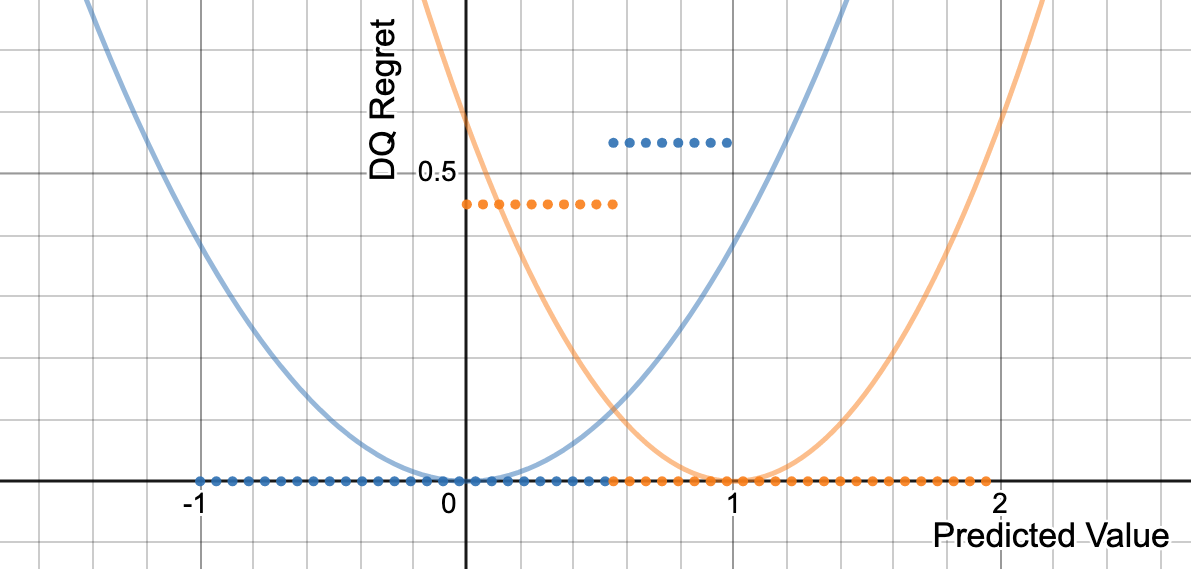
Figure 1: A plot of vs. (for fixed ). The samples from Step 1 correspond to the blue dots for the instance and the orange dots for the instance. We also plot the learned weighted MSE loss for each instance using solid lines in their corresponding colors. -
3.
Based on this dataset, we fit a loss of the form given by Equation 3. Because there is only one weight being learned here, this can be seen as either a WeightedMSE LODL from Shah et al. [15] or a reweighted task-loss from Lawless and Zhou [9]. This leads to the loss seen in Figure 1.
-
4.
Finally, we estimate a predictive model based on this loss. The optimal prediction given this loss is (see Appendix B for details).
Importantly, under this predictive model, the optimal decision would be to give the resource to individual because they have higher predicted utility, i.e., . But this is suboptimal!
5 EGLs (Part One): Feature-based Parameterization
The challenge of learning the function is that it is as hard as learning a closed-form solution to an arbitrary optimization problem in the worst case. To get around this, past approaches typically learn multiple local approximations e.g., for every decision-making instance in the training and validation set. This simplification trades off the complexity of learning a single complex for the cost of learning many simpler functions. Specifically, learning each local requires its own set of samples which can require as many as samples (for the ‘DirectedQuadratic’ loss function from Shah et al. [15]). This is especially problematic because calculating for each of the sampled predictions is the most expensive step in learning task-focused loss functions.
To make this approach more scalable, we propose learning a mapping from the features of a given prediction to the corresponding loss function parameter(s), which we call feature-based parameterization (FBP). This allows us to get the best of both worlds—we retain the simplicity of learning local loss functions while still being able to generalize across different decision-making instances. In fact, our approach even allows for generalization within problem instances as we learn mappings from individual features to their corresponding parameters.
Concretely, we learn the mapping for LODLs loss families in the following way:
-
•
WeightedMSE: We learn a mapping from the features of a prediction to the ‘weight’ that prediction is associated with in the loss function.
-
•
Quadratic: For every pair of predictions and , we learn a mapping where is the matrix that parameterizes the loss function (see Equation 4).
-
•
Directed Variants: Instead of learning a mapping from the features to a single parameter, we instead learn a mapping from for ‘Directed WeightedMSE’ and for ‘Directed Quadratic’.
We then optimize for the optimal parameters of the learned losses along the lines of past work:
where is the learned loss function. For our experiments, the model is a 4-layer feedforward neural network with a hidden dimension of 500 trained using gradient descent.
We’d like to acknowledge here that FBP reduces the expressivity of our learned losses—it implicitly asserts that two predictions with similar features must have a similar impact on the decision quality regret . However, we find in our experiments that this trade-off is typically beneficial. In fact, we show in the section below that this reduction in expressivity is even desirable in some ways.
5.1 Fisher Consistency
One desirable property of a Predict-then-Optimize loss function is that, in the limit of infinite data and model capacity, the optimal prediction induced by the loss also minimizes the decision quality regret. If this is true, we say that loss is "Fisher Consistent" w.r.t. the decision quality regret [6].
Definition 5.1 (Fisher Consistency).
A loss is said to be Fisher Consistent with respect to the decision quality regret if the set of minimizers of the loss function also minimize for all possible distributions .
However, the methods proposed in past work do not satisfy this property even for the simplest of cases—in which the objective of the optimization problem is linear. Concretely:
Proposition 5.2.
Weighting-the-MSE losses are not Fisher Consistent for Predict-then-Optimize problems in which the optimization function has a linear objective.
Proof.
See the counterexample in Section 4. ∎
More generally, because ‘WeightedMSE’ can be seen as a special case of the other methods in Shah et al. [15], none of the loss functions in past work are Fisher Consistent! To gain an intuition for why this happens, let us analyze the predictions that are induced by weighting-the-MSE type losses:
Lemma 5.3.
The optimal prediction for some feature given a weighted MSE loss function with weights associated with the label is , given infinite model capacity.
The proof is presented in Appendix A. In their paper, Elmachtoub and Grigas [6] show that the optimal prediction that minimizes is , i.e., the optimal prediction should depend only on the value of the labels corresponding to that feature. However, in weighted MSE losses, and so the optimal prediction depends on not only the labels but also the weight associated with them. While this is not a problem by itself, the weight learned for a label is dependent on not only the label itself but also the other labels in that instance. In the context of the Section 4 example, the weight associated with individual is dependent on the utility of individual (via ). As a result, it’s possible to create a distribution for which such losses will not be Fisher Consistent. However, this is not true for WeightedMSE with FBP!
Theorem 5.4.
WeightedMSE with FBP is Fisher Consistent for Predict-then-Optimize problems in which the optimization function has a linear objective.
Proof.
In WeightedMSE with FBP, the weights associated with some feature are not independently learned for each instance but are instead a function of the features . As a result, the weight associated with that feature is the same across all instances, i.e., , . Plugging that into the equation from Lemma 5.3:
which is a minimizer of [6]. Thus, WeightedMSE with FBP is always Fisher Consistent. ∎
6 EGLs (Part Two): Model-based Sampling
Loss functions serve to give feedback to the model. However, to make them easier to learn, their expressivity is often limited. As a result, they cannot estimate accurately for all possible predictions but must instead concentrate on a subset of "realistic predictions" for which the predictive model will require feedback during training. However, there is a chicken-and-egg problem in learning loss functions on realistic predictions—a model is needed to generate such predictions, but creating such a model would in turn require its own loss function to train on.
Past work has made the assumption that the predictions will be close to the actual labels to efficiently generate potential predictions . However, if the assumption does not hold, Gaussian sampling may not yield good results, as seen in Section 6.1. Instead, in this paper, we propose an alternative: model-based sampling (MBS). Here, to generate a distribution of potential predictions using this approach, we train a predictive model on a standard loss function (e.g., MSE). Then, at equally spaced intervals during the training process, we use the intermediate model to generate predictions for each problem instance in the dataset. These form the set of potential predictions based on which we create the dataset and learn loss functions. In the context of the meta-algorithm from Section 2.2, this changes only Step 1 of the approach. The hyperparameters associated with this approach are:
-
•
Number of Models: Instead of sampling predictions from just one model, we can instead train multiple models to increase the diversity of the generated predictions. In our experiments, we choose from predictive models.
-
•
LR and Number of Training Steps: The learning rates are chosen from with a possible cyclic schedule [16]. We use a maximum of updates across all the models.
We choose from among these different hyperparameter values using iterations of random search interleaved with manual extrapolations of promising combinations. We find that for best performance with MBS, a high learning rate and large number of models works best. Both of these choices increase the diversity of the generated samples and help create a richer dataset for learning loss functions.
6.1 Localness of Predictions
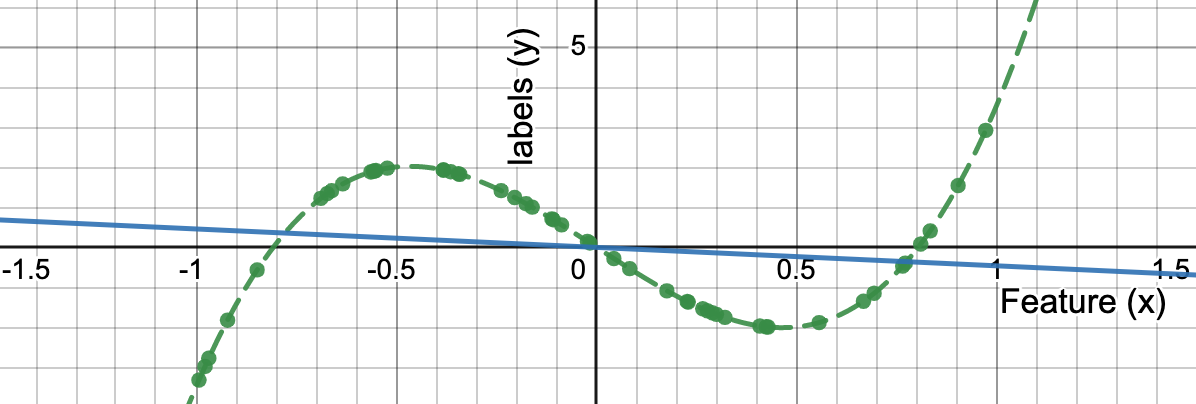
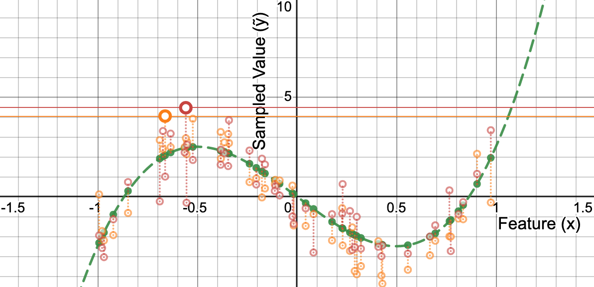
To illustrate the utility of model-based sampling, we analyze the Cubic Top-K domain proposed by Shah et al. [15]. The goal in this domain is to fit a linear model to approximate a more complex cubic relationship between and (Figure 2, Appendix C). This could be motivated by explainablity [14, 8], data efficiency, or simplicity. The localness assumption breaks here because it is not possible for linear models (or low-capacity models more generally) to closely approximate the true labels of a more complex data-generating process. The objective of the learned loss function, then, is to provide information about what kind of suboptimal predictions are better than others.
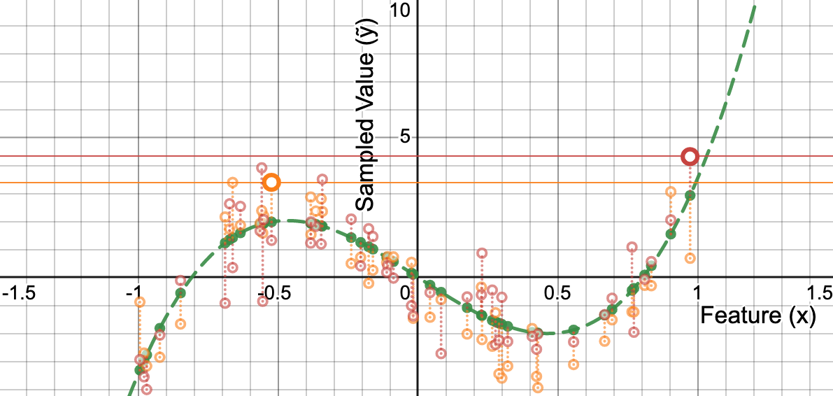
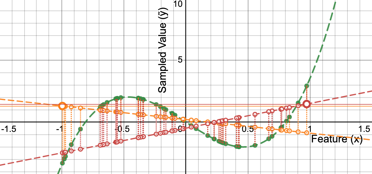
Learned losses accomplish this by first generating plausible predictions and then learning how different sorts of errors change the decision quality. In this domain, the decision quality is solely determined by the point with the highest predicted utility. As can be seen in Figure 2, the highest values given are either at or . In fact, because the function is flatter around , there are more likely to be large values there. When Gaussian sampling [15] is used to generate candidate predictions, the highest sampled values are also more likely to be at because the added noise has a mean of zero. However, a linear model cannot have a maximum value at ; it can only have a maxima at the extremes, i.e., either or . As a result, the loss functions learned based on the samples from this method focus on the wrong subset of labels and lead to poor downstream performance. On the other hand, when using model-based sampling, the generated candidate predictions are the outputs of a linear model. Consequently, the samples generated by this method have maximas only at , allowing the loss functions to take this into account. We visualize this phenomenon in Figure 3 (Appendix C).
In their paper, Shah et al. [15] propose a set of ‘directed models’ to make LODLs perform well in this domain. However, these models only learn useful loss functions because the value of the label at is slightly higher than the value at . To show this, we create a variant of this domain called “(Hard) Cubic Top-K” in which . In Section 7.1 we show that, in this new domain, even the ‘directed’ LODLs fail catastrophically while all the loss functions learned with model-based sampling perform well.
7 Experiments
In this section, we validate EGLs empirically on four domains from the literature. We provide brief descriptions of the domains below but refer the reader to the corresponding papers for more details.
Cubic Top-K [15] Learn a model whose top-k predictions have high corresponding true labels.
-
•
Predict: Predict resource ’s utility using a linear model with feature . The true utility is for the standard version of the domain and for the ‘hard’ version. The predictive model is linear, i.e., .
-
•
Optimize: Out of resources, choose the top resources with highest utility.
Web Advertising [21] The objective of this domain is to predict the Click-Through-Rates (CTRs) of different (user, website) pairs such that good websites to advertise on are chosen.
-
•
Predict: Predict the CTRs for fixed users on websites using the website’s features . The features for each website are obtained by multiplying the true CTRs from the Yahoo! Webscope Dataset [24] with a random matrix , resulting in . The predictive model is a 2-layer feedforward network with a hidden dimension of 500.
-
•
Optimize: Choose which websites to advertise on such that the expected number of users who click on an advertisement at least once (according to the CTR matrix) is maximized. The optimization function to be maximized is , where can be either 0 or 1. This is a submodular maximization problem.
Portfolio Optimization [5, 18] Based on the Markovitz model [10], the aim is to predict future stock prices in order to create a portfolio that has high returns but low risk.
-
•
Predict: Predict the future stock price for each stock using its historical data . The historical data includes information on 50 stocks obtained from the QuandlWIKI dataset [13]. The predictive model is a 2-layer feedforward network with a hidden dimension of 500.
-
•
Optimize: Choose a distribution over stocks to maximize based on a known correlation matrix of stock prices. Here, represents the constant for risk aversion.
For each set of experiments, we run 10 experiments with different train-test splits, and randomized initializations of the predictive model and loss function parameters. Details of the computational resources and hyperparameter optimization used are given in Appendix E.
For all of these domains, the metric of interest is the decision quality achieved by the predictive model on the hold-out test set when trained with the loss function in question. However, given that the scales of the decision quality for each domain vary widely, we linearly re-scale the value such that 0 corresponds to the DQ of making predictions uniformly at random and 1 corresponds to making perfect predictions . Concretely:
7.1 Overall Results
We compare our approach against the following baselines from the literature in Table 1:
-
•
MSE: A standard regression loss.
-
•
Expert-crafted Surrogates: The end-to-end approaches described in Section 3 that require handcrafting differentiable surrogate optimization problems for each domain separately.
- •
-
•
LODL: Shah et al. [15]’s approach for learning loss functions. Trained using 32 and 2048 samples.
| Category | Method | New Domain | Domains from the Literature | ||
| (Hard) Cubic Top-K | Cubic Top-K | Web Advertising | Portfolio Optimization | ||
| 2-Stage | MSE | -0.65 0.04 | -0.50 0.06 | 0.60 0.04 | 0.04 0.00 |
| Expert-crafted Surrogates | SPO+ [6] | -0.68 0.00 | 0.96 0.00 | - | - |
| Entropy-Regularized Top-K [23] | 0.24 0.08 | 0.96 0.00 | - | - | |
| Multilinear Relaxation [22] | - | - | 0.74 0.01 | - | |
| Differentiable QP [5, 18] | - | - | - | 0.141 0.003 | |
| Learned Losses | L&Z [9, 4] (1 Sample) | -0.68 0.00 | -0.96 0.00 | 0.65 0.02 | 0.133 0.005 |
| LODL [15] (32 Samples) | -0.68 0.00 | -0.38 0.29 | 0.84 0.04 | 0.146 0.003 | |
| LODL [15] (2048 Samples) | -0.67 0.01 | 0.96 0.00 | 0.93 0.01 | 0.154 0.005 | |
|
EGL |
0.69 0.00 | 0.96 0.00 | 0.95 0.01 | 0.153 0.004 | |
(Hard) Cubic Top-K We empirically verify our analysis from Section 6.1 by testing different baselines on our proposed ‘hard’ top-k domain. In Table 1, we see that all our baselines perform extremely poorly in this domain. Even the expert-crafted surrogate only achieves a DQ of while EGLs achieve the best possible DQ of ; this corresponds to a gain of nearly 200% for EGLs.
Domains for the Literature We find that our method reaches state-of-the-art performance in all the domains from the literature. In fact, we see that EGLs achieve similar performance to LODLs with an order of magnitude fewer samples in two out of three domains. In Section 7.2 below, we see that this corresponds to an order of magnitude speed-up over learning LODLs of similar quality!
7.2 Computational Complexity Experiments
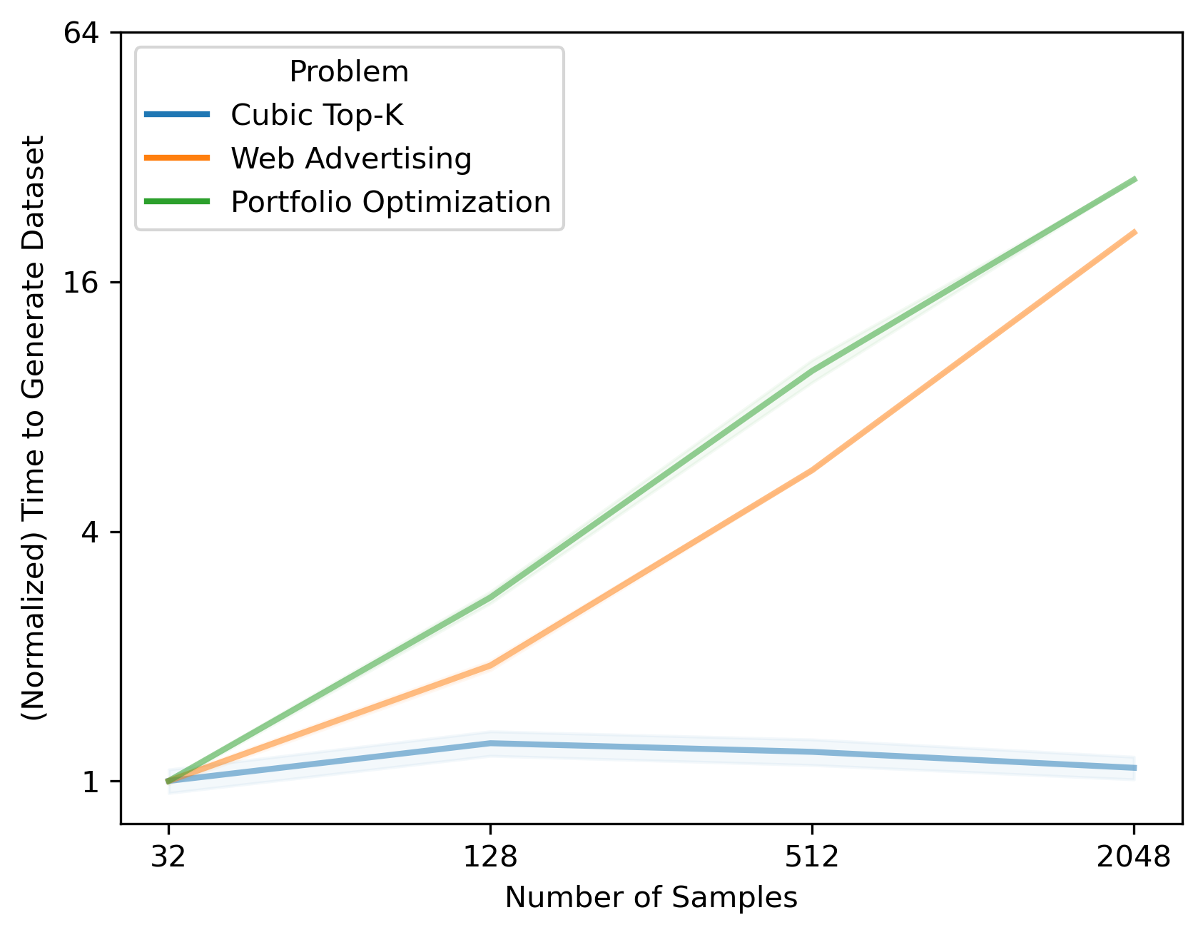
We saw in Section 7.1 that EGLs perform as well as LODLs with an order of magnitude fewer samples. In Table 2, we show how this increased sample efficiency translates to differences in runtime. We see that, by far, most of the time in learning LODLs is spent in ‘Step 2’ of our meta-algorithm. As a result, despite the fact that EGLs take longer to perform steps 1 and 3, this is made up for by the increase in sample efficiency, resulting in an order-of-magnitude speedup over LODLs.
| Method | Time Taken Per Step (in seconds) | Total Time (in seconds) | ||
| Step 1: Samping | Step 2: Generating Dataset | Step 3: Learning Losses | ||
| LODL | 0.18 0.01 (Gaussian Sampling) | 10376.65 119.81 (2048 samples) | 53.67 1.84 (Separate Losses) | 10430.50 131.66 |
| EGL |
0.48 0.04 (MBS) | 200.43 4.24 (32 samples) | 445.67 62.42 (FBP) | 646.58 66.70 |
7.3 Ablation Study
| Domain | Method | Normalized Test Decision Quality | |||
| Directed Quadratic | Directed WeightedMSE | Quadratic | WeightedMSE | ||
| Cubic Top-K | LODL | -0.38 0.29 | -0.86 0.10 | -0.76 0.19 | -0.95 0.01 |
| LODL (2048 samples) | -0.94 0.01 | 0.96 0.00 | -0.95 0.01 | -0.96 0.00 | |
| EGL (MBS) | 0.96 0.00 | 0.96 0.00 | 0.77 0.13 | 0.77 0.13 | |
| EGL (FBP) | 0.58 0.26 | 0.96 0.00 | -0.28 0.21 | -0.77 0.11 | |
| EGL (Both) | 0.96 0.00 | 0.77 0.13 | 0.96 0.00 | 0.77 0.13 | |
| Web Advertising | LODL | 0.75 0.05 | 0.72 0.03 | 0.84 0.04 | 0.71 0.03 |
| LODL (2048 samples) | 0.93 0.01 | 0.84 0.02 | 0.93 0.01 | 0.78 0.03 | |
| EGL (MBS) | 0.86 0.03 | 0.83 0.03 | 0.78 0.06 | 0.77 0.04 | |
| EGL (FBP) | 0.93 0.02 | 0.80 0.03 | 0.92 0.01 | 0.75 0.04 | |
| EGL (Both) | 0.95 0.01 | 0.78 0.06 | 0.92 0.02 | 0.81 0.04 | |
| Portfolio Optimization | LODL | 0.146 0.003 | 0.136 0.003 | 0.145 0.003 | 0.122 0.003 |
| LODL (2048 samples) | 0.154 0.005 | 0.141 0.004 | 0.147 0.004 | 0.113 0.014 | |
| EGL (MBS) | 0.135 0.011 | 0.138 0.010 | 0.146 0.015 | 0.108 0.009 | |
| EGL (FBP) | 0.139 0.005 | 0.141 0.008 | 0.147 0.008 | 0.136 0.004 | |
| EGL (Both) | 0.134 0.013 | 0.127 0.011 | 0.145 0.011 | 0.153 0.004 | |
In this section, we compare EGLs to their strongest competitor from the literature, i.e., LODLs [15]. Specifically, we look at the low-sample regime—when 32 samples per instance are used to train both losses—and present our results in Table 3. We see that EGLs improve the decision quality for almost every choice of loss function family and domain. We further analyze Table 3 below.
Feature-based Parameterization (FBP): Given that this is the low-sample regime, ‘LODL + FBP’ almost always does better than just LODL. These gains are especially apparent in cases where adding more samples would improve LODL performance—the ‘Directed’ variants in the Cubic Top-K domain, and the ‘Quadratic’ methods in the Web Advertising domain.
Model-based Sampling (MBS): This contribution is most useful in the Cubic Top-K domain, where the localness assumption is broken. Interestingly, however, MBS also improves performance in the other two domains where the localness assumption does not seem to be broken (Table 4 in Section E.1). We hypothesize that MBS helps here in two different ways:
-
1.
Increasing effective sample efficiency: We see that, in the cases where FBP helps most, the gains from MBS stack with FBP. This suggests that MBS helps improve sample-efficiency. Our hypothesis is that model-based sampling allows us to focus on predictions that would lead to a ‘fork in the training trajectory’, leading to improved performance with fewer samples.
-
2.
Helping WeightedMSE models: MBS also helps improve the worst-performing WeightedMSE models in these domains which, when combined with FBP, outperform even LODLs with 2048 samples. This suggests that MBS does more than just increase sample efficiency. We hypothesize that MBS also reduces the search space by limiting the set of samples to ‘realistic predictions’, allowing even WeightedMSE models that have fewer parameters to perform well in practice.
Portfolio Optimization: The results for this domain don’t follow the trends noted above because there is distribution shift between the validation and test sets in this domain (as the train/test/validation split is temporal instead of i.i.d.). In Table 5 (Section E.2), we see that EGLs significantly outperform LODLs and follow the trends noted above if we measure their performance on the validation set, which is closer in time to training (and hence has less distribution shift).
References
- Agrawal et al. [2019] Akshay Agrawal, Brandon Amos, Shane Barratt, Stephen Boyd, Steven Diamond, and J Zico Kolter. Differentiable convex optimization layers. Advances in Neural Information Processing Systems, 32, 2019.
- Amos et al. [2018] Brandon Amos, Ivan Jimenez, Jacob Sacks, Byron Boots, and J. Zico Kolter. Differentiable mpc for end-to-end planning and control. In Advances in Neural Information Processing Systems, volume 31, 2018.
- Bengio [1997] Yoshua Bengio. Using a financial training criterion rather than a prediction criterion. International journal of neural systems, 8(04):433–443, 1997.
- Chung et al. [2022] Tsai-Hsuan Chung, Vahid Rostami, Hamsa Bastani, and Osbert Bastani. Decision-aware learning for optimizing health supply chains. arXiv preprint arXiv:2211.08507, 2022.
- Donti et al. [2017] Priya Donti, Brandon Amos, and J Zico Kolter. Task-based end-to-end model learning in stochastic optimization. Advances in Neural Information Processing Systems, 30, 2017.
- Elmachtoub and Grigas [2021] Adam N Elmachtoub and Paul Grigas. Smart “predict, then optimize”. Management Science, 2021.
- Ferber et al. [2020] Aaron Ferber, Bryan Wilder, Bistra Dilkina, and Milind Tambe. MIPaaL: Mixed integer program as a layer. In Proceedings of the AAAI Conference on Artificial Intelligence, volume 34, pages 1504–1511, 2020.
- Hughes et al. [2018] Michael Hughes, Gabriel Hope, Leah Weiner, Thomas McCoy, Roy Perlis, Erik Sudderth, and Finale Doshi-Velez. Semi-supervised prediction-constrained topic models. In Proceedings of the Twenty-First International Conference on Artificial Intelligence and Statistics, pages 1067–1076, 2018.
- Lawless and Zhou [2022] Connor Lawless and Angela Zhou. A note on task-aware loss via reweighing prediction loss by decision-regret. arXiv preprint arXiv:2211.05116, 2022.
- Markowitz and Todd [2000] Harry M Markowitz and G Peter Todd. Mean-variance analysis in portfolio choice and capital markets. John Wiley & Sons, 2000.
- Mensch and Blondel [2018] Arthur Mensch and Mathieu Blondel. Differentiable dynamic programming for structured prediction and attention. In International Conference on Machine Learning, pages 3462–3471. PMLR, 2018.
- Mulamba et al. [2021] Maxime Mulamba, Jayanta Mandi, Michelangelo Diligenti, Michele Lombardi, Victor Bucarey, and Tias Guns. Contrastive losses and solution caching for predict-and-optimize. In Proceedings of the International Joint Conferences on Artificial Intelligence, 2021.
- Quandl [2022] Quandl. WIKI various end-of-day data, 2022. URL https://www.quandl.com/data/WIKI.
- Rudin [2019] Cynthia Rudin. Stop explaining black box machine learning models for high stakes decisions and use interpretable models instead. Nature Machine Intelligence, 1(5):206–215, 2019.
- Shah et al. [2022] Sanket Shah, Kai Wang, Bryan Wilder, Andrew Perrault, and Milind Tambe. Decision-focused learning without decision-making: Learning locally optimized decision losses. In Advances in Neural Information Processing Systems, 2022.
- Smith [2017] Leslie N Smith. Cyclical learning rates for training neural networks. In 2017 IEEE winter conference on applications of computer vision (WACV), pages 464–472. IEEE, 2017.
- Tschiatschek et al. [2018] Sebastian Tschiatschek, Aytunc Sahin, and Andreas Krause. Differentiable submodular maximization. In Proceedings of the 27th International Joint Conference on Artificial Intelligence, pages 2731–2738, 2018.
- Wang et al. [2020] Kai Wang, Bryan Wilder, Andrew Perrault, and Milind Tambe. Automatically learning compact quality-aware surrogates for optimization problems. Advances in Neural Information Processing Systems, 33:9586–9596, 2020.
- Wang et al. [2021] Kai Wang, Sanket Shah, Haipeng Chen, Andrew Perrault, Finale Doshi-Velez, and Milind Tambe. Learning mdps from features: Predict-then-optimize for sequential decision making by reinforcement learning. In M. Ranzato, A. Beygelzimer, Y. Dauphin, P.S. Liang, and J. Wortman Vaughan, editors, Advances in Neural Information Processing Systems, volume 34, pages 8795–8806. Curran Associates, Inc., 2021. URL https://proceedings.neurips.cc/paper_files/paper/2021/file/49e863b146f3b5470ee222ee84669b1c-Paper.pdf.
- Wang et al. [2022] Kai Wang, Shresth Verma, Aditya Mate, Sanket Shah, Aparna Taneja, Neha Madhiwalla, Aparna Hegde, and Milind Tambe. Decision-focused learning in restless multi-armed bandits with application to maternal and child care domain. arXiv preprint arXiv:2202.00916, 2022.
- Wilder et al. [2019a] Bryan Wilder, Bistra Dilkina, and Milind Tambe. Melding the data-decisions pipeline: Decision-focused learning for combinatorial optimization. In Proceedings of the AAAI Conference on Artificial Intelligence, volume 33, pages 1658–1665, 2019a.
- Wilder et al. [2019b] Bryan Wilder, Eric Ewing, Bistra Dilkina, and Milind Tambe. End to end learning and optimization on graphs. Advances in Neural Information Processing Systems, 32:4672–4683, 2019b.
- Xie et al. [2020] Yujia Xie, Hanjun Dai, Minshuo Chen, Bo Dai, Tuo Zhao, Hongyuan Zha, Wei Wei, and Tomas Pfister. Differentiable top-k with optimal transport. Advances in Neural Information Processing Systems, 33:20520–20531, 2020.
- Yahoo! [2007] Yahoo! Webscope dataset, 2007. URL https://webscope.sandbox.yahoo.com/. ydata-ysm-advertiser-bids-v1.0.
Appendix A Proof of Lemma 5.3
Proof.
The loss value for a prediction made using features for a weight-the-MSE type loss is:
To find the optimal prediction, we differentiate the RHS with respect to the prediction corresponding to the feature and equate it to . Importantly, the prediction is not dependent on the distributions . Moreover, because we assume infinite model capacity, the prediction can also take any value and is independent of any other prediction . As a result:
∎
Appendix B Numerical Details for the Motivating Example in Section 4
We give more numerical details for the motivating example step-wise below:
-
•
Step 1: For each instance, and , we generate 15 possible predictions by adding noise to and respectively. Concretely, we consider the following possible predictions , and .
-
•
Step 2: For each of these possible predictions, we calculate the optimal decision and then the decision quality regret . We document these values in the following table:
Possible Predicted Utilities Optimal Decision Decision Quality Regret (-1, 0.55) Give Resource to B 9 values ⋮ ⋮ ⋮ (0.43, 0.55) Give Resource to B (0.57, 0.55) Give Resource to A 2 values ⋮ ⋮ ⋮ (1, 0.55) Give Resource to A (0, 0.55) Give Resource to B 2 values ⋮ ⋮ ⋮ (0.43, 0.55) Give Resource to B (0.57, 0.55) Give Resource to A 9 values ⋮ ⋮ ⋮ (2, 0.55) Give Resource to A -
•
Step 3: Based on the datasets and for each instance, we learn weights for the corresponding instance by learning a weight for each instance that minimizes the MSE loss. Specifically, we choose:
To calculate the we run gradient descent, and get and .
-
•
Step 4: Based on Lemma 5.3, we know that:
Then, plugging the values of the weights from Step 3 into the formula above, we get:
Appendix C Visualizations for the Cubic Top-K domain
Appendix D Limitations
-
•
Smaller speed-ups in simple decision-making tasks: In Section 7.2 we show how a reduction in the number of samples needed to train loss functions almost directly corresponds to a speed-up in learning said losses. This is because Step 2 of the meta-algorithm (Section 2.2), in which we have to run an optimization solver for multiple candidate predictions, is the rate-determining step. However, for simpler optimization problems that can be solved more quickly (e.g., the Cubic Top-K domain in Figure 4), this may no longer be the case. In that case, FBP is likely to have limited usefulness. Conversely, however, FBP is likely to be even more beneficial for more complex decision-making problems (e.g., MIPs [7] or RL tasks [19]).
-
•
Limited Understanding of Why MBS Performs Well: In this paper, we endeavor to provide necessary conditions for when MBS allows EGLs to outperform LODLs, i.e., when the localness assumption is broken. However, EGLs seem to work well even when these conditions do not hold, e.g., in the Web Advertising and Portfolio Optimization domains. We provide hypotheses for why we believe this occurs in Section 7.3, but further research is required to rigorously test them.
Appendix E Additional Results
We run our experiments on an internal cluster. Each job was run with up to 16GM of memory, 8 cores of an Intel Xeon Cascade Lake CPUs, and optionally one Nvidia A100 GPU. For hyperparameter tuning, we average over 10 different train-test splits and random NN initialization, and choose the set of hyperparameters with the highest Decision Quality on a Validation set.
E.1 Localness of Predictions in Different Domains
| Domain | Final Validation MSE |
| Portfolio Optimization | 0.000402 |
| Web Advertising | 0.063420 |
| Cubic Top-K | 2.364202 |
| (Hard) Cubic Top-K | 3.015765 |
E.2 Analyzing the Portfolio Optimization Domain
| Domain | Method | Normalized Validation Decision Quality | |||
| Directed Quadratic | Directed WeightedMSE | Quadratic | WeightedMSE | ||
| Portfolio Optimization | LODL | 0.170 0.006 | 0.150 0.007 | 0.165 0.006 | 0.134 0.007 |
| LODL (2048 samples) | 0.189 0.009 | 0.162 0.009 | 0.165 0.008 | 0.144 0.014 | |
| EGL (MBS) | 0.171 0.026 | 0.160 0.027 | 0.179 0.047 | 0.140 0.018 | |
| EGL (FBP) | 0.172 0.009 | 0.175 0.030 | 0.170 0.022 | 0.151 0.009 | |
| EGL (Both) | 0.186 0.020 | 0.179 0.024 | 0.190 0.022 | 0.172 0.009 | |
E.3 Time taken to generate dataset for learned losses