An intrinsic causality principle in histories-based quantum theory: a proposal

Fay Dowker^a,b and Rafael D. Sorkin^b,c,d

^aBlackett Laboratory, Imperial College, Prince Consort Road, London, SW7 2AZ, UK
^bPerimeter Institute, 31 Caroline Street North, Waterloo ON, N2L 2Y5, Canada
^cSchool of Theoretical Physics, Dublin Institute for Advanced Studies, 10 Burlington Road, Dublin 4, Ireland
^dDepartment of Physics, Syracuse University, Syracuse, NY 13244-1130, U.S.A.

Abstract

Relativistic causality (RC) is the principle that no cause can act outside its future lightcone, but any attempt to formulate this principle more precisely will depend on the foundational framework that one adopts for quantum theory. Adopting a histories-based (or “path integral”) framework, we relate RC to a condition we term “Persistence of Zero” (PoZ), according to which an event $E$ of measure zero remains forbidden if one forms its conjunction with any other event associated to a spacetime region that is later than or spacelike to that of $E$. We also relate PoZ to the Bell inequalities by showing that, in combination with a second, more technical condition it leads to the quantal counterpart of Fine’s patching theorem in much the same way as Bell’s condition of Local Causality leads to Fine’s original theorem. We then argue that RC per se has very little to say on the matter of which correlations can occur in nature and which cannot. From the point of view we arrive at, histories-based quantum theories are nonlocal in spacetime, and fully in compliance with relativistic causality.

1 Introduction

Causal relationships are important in Quantum Field Theory (QFT), in classical General Relativity (GR), and for Quantum Foundations. Causality appeals to us as a basic scientific category, and yet cause and effect lack a clear definition in quantum physics. There is no consensus on whether EPR-like correlations indicate that quantum physics is nonlocal, or not relativistically causal, or both.

The meaning of cause is elusive, even classically. In quantum mechanics and QFT it is even harder to give it meaning. Causality concerns events in spacetime, whereas the field operators in terms of which one usually formulates the causality conditions (as they are usually described) of relativistic QFT are not events. The only true spacetime event in an operator formulation of a quantum theory is a “measurement” with its ensuing “collapse of the state-vector”, but measurement and collapse rely on external observers in spacetime. Measurement and collapse are needed in the canonical operator-formulation but these concepts are not intrinsic to the quantum system. In terms of the histories of a system (trajectories in quantum mechanics, field configurations in QFT), though, one can meaningfully speak of spacetime events without reference to anything external to the quantum system. It is thus worthwhile to explore questions of causality and locality in the context of a histories-based formulation of quantum dynamics.

Quantum Measure Theory (QMT) is such a framework and within it one has the concept of an event in spacetime as a set of histories [1, 2, 3, 4, 5, 6]. J.B. Hartle’s Generalised Quantum Mechanics (GQM) [7, 8, 9, 10] is a closely related histories-based framework for quantum foundations. The two frameworks GQM and QMT are based on the same concepts of history, of event (called a “coarse-grained history” in the GQM literature), and of decoherence functional, though they diverge in their attitudes to decoherence and probabilities, and in their interpretational schemes. Since the technical results in this article do not depend on an interpretational scheme, they are equally applicable to QMT and GQM.

This article will explore causality and locality in Quantum Measure Theory, and in connection with EPR-type correlations. We will consider only particle trajectories and field configurations on spacetime with no appeal to external observers or agents. Our aim is to provide a dynamical axiom that has some claim to be regarded as a principle of relativistic causality. Thus, relativistic causality will be thought of as restricting a general class of conceivable dynamics to a subclass that deserves to be described as causal. We will assume, however, that spacetime is provided with a fixed, or “background” relativistic causal structure; we will not attack the important questions that arise when causal structure graduates from background to dynamical, as it necessarily does whenever gravity is involved.

We begin in Section 2 by reviewing the basics of the histories-based, path integral inspired framework of Quantum Measure Theory, including the concept of the event Hilbert space of a system. We then specialise to the case of quantum theory in a relativistic spacetime background in Section 3 and introduce the restriction of “Persistence of Zero” on the dynamics of such a quantum system. Persistence of Zero (PoZ) is, as advertised in the title of this article, an intrinsic condition for a quantum theory, not reliant on concepts such as measurement by an external agent. We motivate PoZ by showing that it implies, for each event, $E$, that there exists an event-operator $\hat{E}$ on the event Hilbert space of the past (to be defined), such that $\hat{E}$ acting on the universal vector (also to be defined) produces the vector in the event Hilbert space that corresponds to event $E$. PoZ implies that if an event $E$ has measure zero then the event ‘$E$ and $F$’ also has measure zero whenever $F$ is an event that is nowhere to the past of $E$. We also show that the event-operators for spacelike events commute.

In Section 4 we further support the proposal that PoZ should be considered to be a causality condition. Specifically, we show that, in the case that the event Hilbert space of the whole system equals the event Hilbert space of the past—which condition we call “Lack of Novelty”—PoZ plays the crucial role in the quantal “patching theorem” analogous to that played by the familiar factorizability condition in A. Fine’s original classical version of the theorem [11].

We follow this with two sections of more informal discussion. In Section 5 we argue that relativistic causality, taken in isolation, is a rather weak condition which in particular imposes no limitation on the spacelike correlations that a localized cause can induce among events in its future. We illustrate this by reframing two well-known examples—the Popescu-Rohrlich box and the Greenberger-Horne-Zeilinger experiment—in the language of events, showing that there is nothing about the correlations in either of these cases that warrants the conclusion that relativistic causality is violated. The only residual implication of relativistic causality, then, is that a localized cause should not induce correlations between events that fail to be in its future, and this seems to be what the PoZ condition is aiming to insure. However, as we discuss in section 6, PoZ goes further by incorporating a limited amount of spacetime locality that one might perhaps term as ‘causal severability’, this being one way to think of what the quantal patching theorem expresses.

Finally, Appendix A discusses a quantal analog of classical factorizability that holds in relativistic QFT, and which could conceivably take over the role of Lack of Novelty in an alternative proof of the quantum patching theorem.

2 Quantum measure theory

QMT and GQM are path-integral inspired frameworks in which a quantum system is characterized by a triple, $(\Omega,\mathfrak{A},D)$, consisting of a set of histories $\Omega$, an event algebra $\mathfrak{A}$ (a subalgebra of the power set of $\Omega$), and a decoherence functional $D(\cdot,\cdot)$ on $\mathfrak{A}\times\mathfrak{A}$. In this section we review the basic concepts of history, event and decoherence functional and refer the reader to [1, 2, 3, 4, 5, 6] for more details on QMT, to [7, 8, 9, 10] for more details on GQM, and to [12, 13, 14, 15, 16] for more details on the event Hilbert space and the vector-measure.

2.1 Event Algebra

The kinematics of a quantum system in QMT is specified by the set $\Omega$ of histories and one may have in mind that this is the set of histories over which the path integral is performed. Each history $C$ in $\Omega$ is as complete a description of the physical system as is in principle possible in the theory. For example, in $n$-particle quantum mechanics, a history is a set of $n$ trajectories in spacetime and in a scalar field theory, a history is a real or complex function on spacetime.

Any physical statement about (or property of) the system is a statement about (or property of) the history of the system. And, therefore, the statement/property corresponds to a subset of $\Omega$ in the obvious way. For example, in the case of the non-relativistic particle, if $R$ is a region of spacetime, the statement/property “the particle passes through $R$” corresponds to the set of all trajectories that pass through $R$. We adopt the terminology of stochastic processes in which such subsets of $\Omega$ are referred to as events.

An event algebra on a sample space $\Omega$ is a non-empty collection, ${\mathfrak{A}}$, of subsets of $\Omega$ such that

1. $\Omega\setminus E\in{\mathfrak{A}}$ for all $E\in{\mathfrak{A}}$ (closure under complementation),

2. $E\cup F\in{\mathfrak{A}}$ for all $E,F\in{\mathfrak{A}}$ (closure under finite union).

It follows from the definition that $\emptyset\in{\mathfrak{A}}$, $\Omega\in{\mathfrak{A}}$ and ${\mathfrak{A}}$ is closed under finite intersections. An event algebra is an algebra of sets by a standard definition, and a Boolean algebra. For events qua statements about the system, set operations correspond to logical combinations of statements in the usual way: union is “inclusive or”, intersection is “and”, complementation is “not” etc.

An event algebra ${\mathfrak{A}}$ is also an algebra in the sense of a vector space over a set of scalars, $\mathbb{Z}_{2}$, with intersection as multiplication and symmetric difference (or “boolean sum”) as addition:

• $EF:=E\cap F$, for all $E,F\in{\mathfrak{A}}$;

• $E+F:=(E\setminus F)\cup(F\setminus E)$ , for all $E,F\in{\mathfrak{A}}$.

In this algebra, the unit element, $\mathbb{1}\in{\mathfrak{A}}$, is the whole set of histories $\mathbb{1}:=\Omega$. The zero element, $\mathbb{0}\in{\mathfrak{A}}$, is the empty set $\mathbb{0}:=\emptyset$. Note that $E+F=E\cup F$ if and only if $E$ and $F$ are disjoint i.e. if and only if $EF=\mathbb{0}$. We will use this arithmetic way of expressing set algebraic formulae whenever convenient, both for events and also for regions of spacetime.

If an event algebra ${\mathfrak{A}}$ is also closed under countable unions then ${\mathfrak{A}}$ is a $\sigma$-algebra but we do not impose this extra condition on the event algebra. (See [14, 15, 17] for work on extending the domain of the quantum measure from ${\mathfrak{A}}$ to a larger subset of the $\sigma$-algebra generated by ${\mathfrak{A}}$.)

2.2 Decoherence functional, quantum measure, vector-measure

A decoherence functional on an event algebra ${\mathfrak{A}}$ is a map $D:{\mathfrak{A}}\times{\mathfrak{A}}\to\mathbb{C}$ that encodes both the initial conditions and the dynamics of the quantum system and satisfies the conditions:

1. $D(E,F)=D(F,E)^{*}$ for all $E,F\in{\mathfrak{A}}$ (Hermiticity);

2. $D(E,F+G)=D(E,F)+D(E,G)$ for all $E,F,G\in{\mathfrak{A}}$ s.t. $FG=\mathbb{0}$ (Additivity);

3. $D(\Omega,\Omega)=1$ (Normalisation);

4. $D(E,E)\geq 0$ for all $E\in{\mathfrak{A}}$ (Weak Positivity).

See section 6 of [10] for these axioms in the context of GQM.

A quantum measure on an event algebra ${\mathfrak{A}}$ is a map $\mu:{\mathfrak{A}}\to\mathbb{R}$ such that,

1. $\mu(E)\geq 0$ for all $E\in{\mathfrak{A}}$ (Positivity);

2. $\mu(E+F+G)-\mu(E+F)-\mu(F+G)-\mu(G+E)+\mu(E)+\mu(F)+\mu(G)=0$, for all $E,F,G\in{\mathfrak{A}}$ s.t. $EF=FG=GE=\mathbb{0}$ (Quantum Sum Rule);

3. $\mu(\Omega)=1$ (Normalisation).

If $D:{\mathfrak{A}}\times{\mathfrak{A}}\to\mathbb{C}$ is a decoherence functional then the map $\mu:{\mathfrak{A}}\to\mathbb{R}$ defined by $\mu(E):=D(E,E)$ is a quantum measure. And, conversely, if $\mu$ is a quantum measure on ${\mathfrak{A}}$ then there exists (a non-unique) decoherence functional $D$ such that $\mu(E)=D(E,E)$ [2].

The question of which is the primitive concept, quantum measure or decoherence function, remains open. However, in this article we take the decoherence functional to be the primitive concept because we will assume all quantum systems satisfy the further axiom of strong positivity which – at our current level of understanding – can only be directly imposed on the decoherence functional:

Definition 1 (Strong Positivity).

A decoherence functional $D:{\mathfrak{A}}\times{\mathfrak{A}}\to{\mathbb{C}}$ is strongly positive if, for each finite set of events $\{E_{1},\dots E_{m}\}$ the corresponding $m\times m$ Hermitian matrix $M_{ij}:=D(E_{i},E_{j})$ is positive semi-definite.

Strong positivity of the decoherence functional holds in established unitary quantum theories due to the form of the decoherence functional as a Double Path Integral (DPI) of Schwinger-Keldysh form, see for example equation (47) in Appendix A. More generally, it has been shown that the set of strongly positive quantum-measure systems is the unique set that is closed under tensor-product composition and is “full” in the sense that if a system can be composed with every element of the set, then that system is in the set [18].

2.3 Event Hilbert space and vector-measure

Henceforth in this article all quantum systems are assumed to have strongly positive decoherence functionals. Then, for each quantum system $(\Omega,{\mathfrak{A}},D)$ a Hilbert space, ${\mathfrak{H}}$, can be constructed as the completion of a quotient of the free vector space over the event algebra [12, 13], such that for each event, $E\in{\mathfrak{A}}$, there is an event-vector $|E\rangle\in{\mathfrak{H}}$ such that:

• $\langle E\,|\,F\rangle=D(E,F),\ \forall E,F\in{\mathfrak{A}}$;

• $|E+F\rangle=|E\rangle+|F\rangle,\ \forall$ $E,F\in{\mathfrak{A}}$ s.t. $EF=\mathbb{0}$;

• ${\mathfrak{H}}$ is spanned by $\{|E\rangle\}_{E\in{\mathfrak{A}}}$. This spanning set is (very) over-complete: there is not a unique expansion of a vector in ${\mathfrak{H}}$ as a linear combination of event-vectors (see, for example, the previous point).

We call this Hilbert space, ${\mathfrak{H}}$, the event Hilbert space. The corresponding map $|\cdot\rangle:{\mathfrak{A}}\rightarrow{\mathfrak{H}}$ is called the quantum vector-measure on the event algebra [12, 13, 14, 15, 16].

• An event has quantum measure zero if and only if its vector-measure is zero.

• If ${\mathfrak{B}}$ is a subalgebra of ${\mathfrak{A}}$ then the event Hilbert space of ${\mathfrak{B}}$ is a subspace of the event Hilbert space of ${\mathfrak{A}}$.

• The vector-measure $|\Omega\rangle$ of the whole history space $\Omega$ is a unit vector in ${\mathfrak{H}}$, and we call it the universal vector. If ${\mathfrak{B}}$ is a (unital) subalgebra of ${\mathfrak{A}}$ then the universal vector is in the event Hilbert space of ${\mathfrak{B}}$. The minimal subalgebra of ${\mathfrak{A}}$ is $\{\Omega,\mathbb{0}\}$, and its event Hilbert space is the 1-d vector space spanned by $|\Omega\rangle$.

• In a unitary quantum theory in which the decoherence functional is defined using the Schwinger-Keldysh double path integral with a pure initial state, the event Hilbert space coincides with the canonical Hilbert space. In this case, the universal vector $|\Omega\rangle$ in the event Hilbert space is identified with the pure initial state in the canonical Hilbert space. If the decoherence functional is defined using a mixed initial state or “density matrix” $\rho$ of rank $r$ then the event Hilbert space is a direct sum of $r$ copies of the canonical Hilbert space. The universal vector $|\Omega\rangle$ is then the direct sum of the eigenvectors of $\rho$, each normalised so that its norm squared is its eigenvalue [13].

• If $X$ is a family of events that constitute a partition of $\Omega$ then

  $$\sum_{E\in X}|E\rangle=|\sum_{E\in X}E\rangle=|\Omega\rangle\,.$$ (1)

3 Spacetime as an organising principle

Our concern is relativistic quantum physics and we assume that the histories of the system, the elements of $\Omega$, reside in a fixed spacetime endowed with a causal structure that is mathematically a partial order. Any “back reaction” on the spacetime metric or causal structure is thus being ignored. This background may be a continuum such as a 4-d globally hyperbolic spacetime or it may be a discrete partial order such as a causal set.

Let us call this spacetime $M$, and its causal order-relation $\preceq$. The availability of this invariable substratum lets us organise events in ${\mathfrak{A}}$ according to their location in $M$. For each spacetime region $R\subseteq M$ there is a subalgebra ${\mathfrak{A}}_{R}\subseteq{\mathfrak{A}}$, where an event $E$ is in ${\mathfrak{A}}_{R}$ iff the property that defines whether a history $\Gamma\in\Omega$ is in $E$ or not is a property of $\Gamma$ in region $R$. In other words, if one can tell whether $\Gamma$ is in $E$ or not by examining the restriction of $\Gamma$ to $R$ then $E$ is in ${\mathfrak{A}}_{R}$, otherwise it is not. We say ‘event $E$ is in region $R$’ to mean the same thing as ‘$E$ is an element of algebra ${\mathfrak{A}}_{R}$’. For each spacetime region $R$, the vector-measures of the events in ${\mathfrak{A}}_{R}$ span a subspace of the event Hilbert space: thus to each region corresponds a sub-Hilbert space ${\mathfrak{H}}_{R}$ of ${\mathfrak{H}}$. If two events are located in mutually spacelike regions, we will say that they are mutually spacelike events.

3.1 Persistence of Zero

Let us consider a spacetime region $R$ and define the region $\bar{R}$ to be the set of points that are not to the causal future of any point in $R$:

$$\bar{R}:=M\setminus J^{+}(R)=\{y\in M:\,\nexists x\in R\ \textit{s.t.}\ x\preceq y\}\,.$$ (2)

Note that $\bar{R}R=\mathbb{0}$, since $R\subseteq J^{+}(R)$.

If the dynamics is relativistically causal, then $\bar{R}$ is the region of spacetime that no event $E$ in $R$ can influence. The question now is whether this informal prohibition can be expressed (at least in part, and subject to later revision when quantum-foundational questions are better clarified) as a condition on the vector-measure of the system.

To that end, let us begin by asking whether it is possible to associate to the event $E$ in $R$, not only a vector in ${\mathfrak{H}}_{R}\subseteq{\mathfrak{H}}$, but an operator on ${\mathfrak{H}}$. We will denote this putative operator by $\widehat{E}$ and refer to it as an event-operator. In the first instance, however, it works better to limit the domain of $\widehat{E}$ to ${\mathfrak{H}}_{\bar{R}}\subseteq{\mathfrak{H}}$.

The Hilbert space ${\mathfrak{H}}_{\bar{R}}$ is spanned by the event-vectors $\{|F\rangle:\,F\in{\mathfrak{A}}_{\bar{R}}\}$. Let $E$ be an event in $R$ and let us try to define a map $\widehat{E}$ from ${\mathfrak{H}}_{\bar{R}}$ to ${\mathfrak{H}}$ by defining it on an arbitrary event-vector in ${\mathfrak{H}}_{\bar{R}}$ as:

$$\widehat{E}|F\rangle:=|EF\rangle\ \ \forall\ F\in{\mathfrak{A}}_{\bar{R}}\,,$$ (3)

and then extending it by linearity to the whole of ${\mathfrak{H}}_{\bar{R}}$. $EF$ is the conjunction event ‘$E$ and $F$’. Given the causal relation between $R$ and $\bar{R}$, although $E$ may be partly or wholly spacelike to $F$, $E$ cannot be to the causal past of $F$; it may therefore help to understand (3) to think of $EF$ as the event ‘$F$ and then $E$’. Now (3) is not necessarily a consistent definition, because the expansion of a vector in ${\mathfrak{H}}_{\bar{R}}$ as a linear combination of event-vectors is not unique. This motivates the following definition:

Definition 2 (Persistence of Zero).

A quantum system satisfies Persistence of Zero (PoZ) if for every region $R$, every finite collection $C$ of events in $\bar{R}$, and every event $E$ in $R$ we have

$$\sum_{F\in C}\psi_{F}|F\rangle=0\implies\sum_{F\in C}\psi_{F}|EF\rangle=0\,,$$ (4)

where $\{\psi_{F}\}$ are complex coefficients.

It is characteristic of quantum theory that a subevent of an event of measure zero can have nonzero measure due to interference: for example in the iconic double slit experiment the measure of the event of the particle arriving at a dark fringe is zero but the measure of the event of the particle passing through the left slit before arriving at a dark fringe is nonzero. But PoZ implies that if an event $F$ has measure zero then any subevent of the form $FE$, where $E$ is an event that is future and/or spacelike to $F$, also has measure zero. So we can already see that PoZ is some sort of causality condition. Moreover, it is just what the definition of $\widehat{E}$ needs for consistency:

Lemma 1.

If a quantum system satisfies PoZ then (3) defines, for each event $E$ in a region $R$ such that $\bar{R}$ is nonempty, a linear map, the event-map $\widehat{E}:{\mathfrak{H}}_{\bar{R}}\rightarrow{\mathfrak{H}}$.

Proof.

The event-vectors in ${\mathfrak{H}}_{\bar{R}}$ span ${\mathfrak{H}}_{\bar{R}}$ and condition PoZ is exactly the condition that $\widehat{E}$ is well defined when extended by linearity to all linear combinations of event-vectors. ∎

Corollary 1.

If a quantum system satisfies PoZ then (3) defines, for each event $E$ in a region $R$ such that $\bar{R}$ is nonempty, and each subregion $Q\subseteq\bar{R}$, the event-map, $\widehat{E}:{\mathfrak{H}}_{Q}\rightarrow{\mathfrak{H}}_{Q+R}$.

Corollary 2.

If a quantum system satisfies PoZ then event-map $\widehat{E}$ acting on the universal vector equals the event-vector for $E$:

$$\widehat{E}|\Omega\rangle=|E\Omega\rangle=|E\rangle\,.$$ (5)

Corollary 3.

If a quantum system satisfies PoZ and $E$ and $F$ are disjoint events in a region $R$ then $\widehat{E+F}=\widehat{E}+\widehat{F}$.

Corollary 4.

If a quantum system satisfies PoZ and $\{E_{1},E_{2}\dots E_{n}\}$ is a collection of events in a region $R$ that is a partition of $\Omega$, then the event-maps $\{\widehat{E}_{1},\widehat{E}_{2},\dots\widehat{E}_{n}\}$ sum to the identity map from ${\mathfrak{H}}_{\bar{R}}$ to ${\mathfrak{H}}_{\bar{R}}$ considered as a subspace of ${\mathfrak{H}}$.

3.2 Spacetime arrangement in the case of interest

In this article we are interested in the following physical setup in spacetime. As shown in figure 1, $Z$ is a region that contains its own causal past: $Z$ is a ‘past set’. Let regions $A$ and $B$ both lie in the future domain of dependence of $Z$ and be disjoint from $Z$ (recall that the future domain of dependence of $Z$ includes $Z$) and be spacelike to each other. The union of regions $Z$, $A$ and $B$ is also a past set. The heuristic justification for this arrangement is that, in a relativistically causal theory, any cause of a correlation between events in $A$ and $B$ must be in $Z$. In particular any “preparation event” in an experiment of EPR type will automatically be contained within the region $Z$.

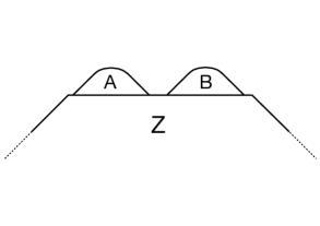
Figure 1: $Z$ is a past set (i.e. contains its own causal past). $A$ and $B$ are in the future domain of dependence of $Z$, do not intersect $Z$ and are spacelike to each other. The union of $Z$, $A$ and $B$ is also a past set.

In unitary quantum field theory in a globally hyperbolic spacetime, the event Hilbert space of the future domain of dependence of $Z$ equals the event Hilbert space of $Z$. For example, if $Z$ is the past of a Cauchy surface then the event Hilbert space of $Z$ and the event Hilbert space of the future domain of dependence of $Z$ both equal the canonical Hilbert space of the whole system.

This can be thought of as a condition of ‘lack of novelty’: the past region $Z$ is rich enough in events that further events anywhere in the future domain of dependence of $Z$ do not add anything new to the physics as encoded in the event Hilbert space. We formalise this condition for quantum measure theories in general:

Definition 3 (Lack of Novelty).

A quantum system satisfies Lack of Novelty (LoN) if, for every region of spacetime $Z$ that contains its own past, the event Hilbert space of the future domain of dependence of $Z$ equals the event Hilbert space of $Z$.

In the case of the regions shown in figure 1 LoN implies that Hilbert spaces ${\mathfrak{H}}_{Z+A}$, ${\mathfrak{H}}_{Z+B}$ and ${\mathfrak{H}}_{Z+A+B}$ all equal ${\mathfrak{H}}_{Z}$, where subscript $Z+A$ refers to the union of regions $Z$ and $A$, and so on. So, for example, if $E_{A}$ is an event in $A$ then there exist complex coefficients $\{\psi_{F}\}$ such that

$$|E_{A}\rangle=\sum_{F\in{\mathfrak{A}}_{Z}}\psi_{F}|F\rangle\,.$$ (6)

Lemma 2.

Let the quantum system satisfy PoZ (definition 2) and LoN (definition 3). Let regions $Z$, $A$ and $B$ be as described in figure 1. If $E_{A}$ is an event in $A$ and $E_{B}$ is an event in $B$, then their respective event-maps, $\widehat{E}_{A}$ and $\widehat{E}_{B}$, are operators on ${\mathfrak{H}}_{Z}$, and they commute.

Proof.

Corollary 1 gives us the event-map $\widehat{E}_{A}:{\mathfrak{H}}_{Z}\rightarrow{\mathfrak{H}}_{Z+A}$. Since ${\mathfrak{H}}_{Z+A}={\mathfrak{H}}_{Z}$, $\widehat{E}_{A}$ is an operator on ${\mathfrak{H}}_{Z}$. Similarly for $\widehat{E}_{B}$. Henceforth we refer to such operators as event-operators.

Then, for each $E_{Z}\in{\mathfrak{A}}_{Z}$,

$$\widehat{E}_{B}\widehat{E}_{A}|E_{Z}\rangle =\widehat{E}_{B}|E_{A}E_{Z}\rangle$$ (7)

$$=|E_{B}E_{A}E_{Z}\rangle$$ (8)

$$=\widehat{E}_{A}\widehat{E}_{B}|E_{Z}\rangle\,.$$ (9)

The first equality follows by applying Corollary 1 to region $A$ and the second equality follows by applying Corollary 1 to region $B$. We also used the fact that multiplication commutes in the Boolean algebra so $E_{B}E_{A}E_{Z}=E_{A}E_{B}E_{Z}$. Since the event-vectors $|E_{Z}\rangle$ span ${\mathfrak{H}}_{Z}$ the result follows.
∎

4 Patching theorems

In this section we prove the quantum analog of Fine’s patching theorem (Proposition 3 of [11]), taking PoZ and LoN as our inputs.

Let us consider, for definiteness and following Fine, the Clauser-Horne-Shimony-Holt (CHSH) scenario [20] with two spin-half particles and two “local experiments”, one in each of two spacelike wings. Each local experiment takes the form of a Stern Gerlach analyzer that admits of two possible orientations or “settings”, and through which the particle emerges in one or the other of two exit beams, the upper beam or the lower beam, where it registers in a detector. This scenario can be generalised to any number of spacelike separated regions with any number of settings per analyzer and any number of beams per setting (the particles might have different spins, or there might be sequences of concatenated beam-splitters), and our results generalise mutatis mutandis.

Let us call the two spacelike separated regions where the local experiments take place $A$ and $B$, and let us call the possible settings, $a$ or $a^{\prime}$ in $A$ and $b$ or $b^{\prime}$ in $B$. We refer to $a$, $a^{\prime}$, $b$ and $b^{\prime}$ as local settings. There are then four possible global settings: $ab$, $ab^{\prime}$, $a^{\prime}b$ and $a^{\prime}b^{\prime}$.

The two spin-half particles are prepared and sent to the analyzers, one particle to $A$ and one particle to $B$. Let $Z$ be a region of spacetime such that $Z$ is a past set and such that $A$ and $B$ lie in the future domain of dependence of $Z$ without intersecting $Z$, and the union of $A$, $B$ and $Z$ is also a past set, as shown in figure 1.

For each local setting, $a$ say for the analyzer in $A$, there are two possible beams in which the particle can be detected and two beam-events, corresponding to the particle being detected in the upper beam (u) and the lower beam (d) respectively. There are four sets of experimental probabilities, one for each global setting:

$$\mathbb{P}^{ab}(ij)\,,\mathbb{P}^{ab^{\prime}}(ij^{\prime})\,,\mathbb{P}^{a^{\prime}b}(i^{\prime}j)\,,\ \textrm{and}\ \mathbb{P}^{a^{\prime}b^{\prime}}(i^{\prime}j^{\prime})\,,$$ (10)

where $i,i^{\prime},j,j^{\prime}$ labels the event of the particle being detected in the upper beam or lower beam (each label taking values $u$ or $d$ respectively) for setting $a,a^{\prime},b,b^{\prime}$ respectively. We use the shortened term “beam-event” to signify the detection of a particle in a particular beam, and as above, we sometimes use a simplified notation in which the labels $i,i^{\prime},j,j^{\prime}$ stand for the beam-events itself.

We now postulate that the four probability distributions are compatible with each other in the sense that $\mathbb{P}^{ab}(j)=\mathbb{P}^{a^{\prime}b}(j)$, etc. These conditions (the so-called no-signalling conditions) signify that the experimental probabilities of the events in $B$ do not depend on the setting in $A$ and vice versa.

The patching theorems are about different measure theories in the same region of spacetime and we will need the following concepts and definitions. For a measure theory in a spacetime $M$ with history-space $\Omega$, if $R\subset M$ is a region of spacetime, then a history in $R$ is an element of $\Omega$ restricted to $R$. We use the notation $\Omega_{R}=\{\Gamma|_{R}:\,\Gamma\in\Omega\}$ for the space of histories restricted to $R$.

Definition 4 (History-event in a region).

Let $R\subseteq M$ be a region of spacetime, a history-event in $R$ is a cylinder set,

$$E_{\gamma_{R}}:=\{\Gamma\in\Omega:\,\Gamma|_{R}=\gamma_{R}\}\,,$$ (11)

where $\gamma_{R}$ is a history in $R$.

Definition 5 (Agreement of measure theories in a region).

Two measure theories, $\{\Omega^{1},{\mathfrak{A}}^{1},D^{1}\}$ and $\{\Omega^{2},{\mathfrak{A}}^{2},D^{2}\}$, in $M$ agree in region $R$ if:

• The two history-spaces restricted to $R$ are equal,

  $$\Omega^{1}_{R}=\Omega^{2}_{R}\,,$$ (12)

  in which case there is an obvious physical isomorphism between ${\mathfrak{A}}^{1}_{R}$ and ${\mathfrak{A}}^{2}_{R}$, the event algebras for the two theories restricted to $R$.

• The decoherence functionals $D^{1}$ and $D^{2}$, restricted to ${\mathfrak{A}}^{1}_{R}$ and ${\mathfrak{A}}^{2}_{R}$ respectively—denoted $D^{1}_{R}$ and $D^{2}_{R}$—are equal via the isomorphism. i.e. if the physical isomorphism is

  $$\phi:{\mathfrak{A}}^{1}_{R}\rightarrow{\mathfrak{A}}^{2}_{R}$$ (13)

  then

  $$D^{1}(E,\bar{E})=D^{2}(\phi(E),\phi(\bar{E}))\,,\ \forall E,\bar{E}\in{\mathfrak{A}}^{1}_{R}\,.$$ (14)

When two measure theories $1$ and $2$ agree in a region $R$, then we can and will henceforth identify the algebras ${\mathfrak{A}}^{1}_{R}$ and ${\mathfrak{A}}^{2}_{R}$ via the physical isomorphism. And then the decoherence functionals are equal in $R$: $D^{1}_{R}=D^{2}_{R}$, and further, the sub-event Hilbert spaces in $R$ are equal: ${\mathfrak{H}}^{1}_{R}={\mathfrak{H}}^{2}_{R}$. Strictly, since ${\mathfrak{H}}^{1}_{R}$ and ${\mathfrak{H}}^{2}_{R}$ are subspaces of different event Hilbert spaces in different theories, they are different spaces but we can and will identify them.

4.1 Fine’s classical patching theorem

In the framework of QMT, a classical theory is a quantum measure theory $(\Omega,{\mathfrak{A}},D)$ that satisfies the additional condition

$$D(E,F)=D(EF,EF)\ \ \forall\ E,F\in{\mathfrak{A}}\,.$$ (15)

In a classical theory, all the information in the decoherence functional is encoded in the measure, $\mu(E)=D(E,E)$, which measure satisfies the Kolmogorov sum rule and is referred to as a classical measure or equivalently as a probability measure. A classical measure theory $(\Omega,{\mathfrak{A}},\mu)$ is a level 1 theory in the hierarchy of measure theories delineated in [2].

Definition 6 (Factorizability).

A classical measure theory $(\Omega,{\mathfrak{A}},\mu)$ on a spacetime $Z+A+B$ where regions $Z$, $A$ and $B$ are as in figure 1, is factorizable if

$$\mu(E_{A}E_{B}E_{\gamma_{Z}})\;\mu(E_{\gamma_{Z}})=\mu(E_{A}E_{\gamma_{Z}})\;\mu(E_{B}E_{\gamma_{Z}})$$ (16)

for all $E_{A}\in{\mathfrak{A}}_{A}$ and $E_{B}\in{\mathfrak{A}}_{B}$ and all history-events $E_{\gamma_{Z}}$ in ${\mathfrak{A}}_{Z}$.

If $\mu(E_{\gamma_{Z}})$ is nonzero, and if we divide through by its square, then this becomes the statement (sometimes called ‘screening off’) that the joint probability of $E_{A}$ and $E_{B}$ factorizes when conditioned on a history-event in $Z$.

Definition 7 (Factorizable model).

A factorizable model for the probabilities (10) in the CHSH scenario is a set of four factorizable classical measure theories in $Z+A+B$, $(\Omega^{\alpha\beta},{\mathfrak{A}}^{\alpha\beta},\mu^{\alpha\beta})$ labelled by the four global settings $\alpha\beta=ab,ab^{\prime},a^{\prime}b,a^{\prime}b^{\prime}$, with the following properties.

• For each local setting, $a,a^{\prime},b$ or $b^{\prime}$, the two theories that share that setting agree (as per definition 5) in the relevant spacetime region: theories $ab$ and $ab^{\prime}$ agree in $Z+A$, theories $a^{\prime}b$ and $a^{\prime}b^{\prime}$ agree in $Z+A$, theories $ab$ and $a^{\prime}b$ agree in $Z+B$, and theories $ab^{\prime}$ and $a^{\prime}b^{\prime}$ agree in $Z+B$. This implies that all four theories agree in $Z$.

• For each local setting, the particle is detected either in the upper beam or in the lower beam. For example, for local setting $a$ let $E^{a}_{u}$ and $E^{a}_{d}$ be the beam-events where we have implemented our declared intention to identify events in regions where theories agree. Then $E^{a}_{u}\cup E^{a}_{d}=\Omega^{ab}$ in measure theory $ab$ and $E^{a}_{u}\cup E^{a}_{d}=\Omega^{ab^{\prime}}$ in measure theory $ab^{\prime}$. Similarly for each of the other local settings: e.g. for setting $a^{\prime}$ we have $E^{a^{\prime}}_{u}\cup E^{a^{\prime}}_{d}=\Omega^{a^{\prime}b}$ in theory $a^{\prime}b$ and $E^{a^{\prime}}_{u}\cup E^{a^{\prime}}_{d}=\Omega^{a^{\prime}b^{\prime}}$ in theory $a^{\prime}b^{\prime}$, and so on.

• Each measure $\mu^{\alpha\beta}$ has the corresponding experimental probabilities $\mathbb{P}^{\alpha\beta}$ (10) as marginals:

  $$\sum_{k}\mu^{ab}(E^{a}_{i}E^{b}_{j}E^{Z}_{\gamma_{k}}) =\mathbb{P}^{ab}(ij)\,,$$

  $$\sum_{k}\mu^{ab^{\prime}}(E^{a}_{i}E^{b^{\prime}}_{j^{\prime}}E^{Z}_{\gamma_{k}}) =\mathbb{P}^{ab^{\prime}}(ij^{\prime})\,,$$

  $$\sum_{k}\mu^{a^{\prime}b}(E^{a^{\prime}}_{i^{\prime}}E^{b}_{j}E^{Z}_{\gamma_{k}}) =\mathbb{P}^{a^{\prime}b}(i^{\prime}j)\,,$$

  $$\sum_{k}\mu^{a^{\prime}b^{\prime}}(E^{a^{\prime}}_{i^{\prime}}E^{b^{\prime}}_{j^{\prime}}E^{Z}_{\gamma_{k}}) =\mathbb{P}^{a^{\prime}b^{\prime}}(i^{\prime}j^{\prime})\,,$$ (17)

  where $k$ labels the histories in $Z$ and $i,j,i^{\prime},j^{\prime}=u,d$.

Now we can state

Theorem 1 (Fine’s patching theorem [11]).

If there exists a factorizable model (Definition 7) for the probabilities (10) then there exists a joint probability measure on all the beam-events and all events in $Z$ that has the four factorizable measures, $\{\mu^{\alpha\beta}\}$ as marginals and that therefore (by (17)) has the probability measures (10) as further marginals.

Proof.

We will use $i,i^{\prime},j,j^{\prime}$ and $k$ as shorthand for the events $E^{a}_{i},E^{a^{\prime}}_{i^{\prime}},E^{b}_{j},E^{b^{\prime}}_{j^{\prime}}$ and $E^{Z}_{\gamma_{k}}$.

First note that due to the agreement of the four measures we have $\mu^{ab}(ik)=\mu^{ab^{\prime}}(ik)$ and so we can define $\mu^{a}(ik):=\mu^{ab}(ik)=\mu^{ab^{\prime}}(ik)$. And similarly for each of the other 3 local settings, $a^{\prime}$, $b$ and $b^{\prime}$. Similarly we can define $\mu(k):=\mu^{ab}(k)=\mu^{a^{\prime}b}(k)=\mu^{ab^{\prime}}(k)=\mu^{a^{\prime}b^{\prime}}(k)$.

Now, define a joint probability measure on all the beam-events and the $Z$-history-event $k$:

$$\mu^{patch}(ii^{\prime}jj^{\prime}k):=\mu^{a}(ik)\mu^{a^{\prime}}(i^{\prime}k)\mu^{b}(jk)\mu^{b^{\prime}}(j^{\prime}k)/\left(\mu(k)\right)^{3}\,.$$ (18)

(18) is well defined since if $\mu(k)=0$ then all the probabilities in the numerator vanish too (in which case we define $\mu^{patch}(ii^{\prime}jj^{\prime}k)$ to equal zero). The factorizability of the four measures $\{\mu^{\alpha\beta}\}$ implies that $\mu^{patch}$ has each of them as marginals. For example,

$$\sum_{i^{\prime}j^{\prime}}\mu^{patch}(ii^{\prime}jj^{\prime}k) =\sum_{i^{\prime}j^{\prime}}\mu^{a}(ik)\mu^{a^{\prime}}(i^{\prime}k)\mu^{b}(jk)\mu^{b^{\prime}}(j^{\prime}k)\left(\mu(k)\right)^{-3}$$ (19)

$$=\mu^{a}(ik)\mu^{a^{\prime}}(k)\mu^{b}(jk)\mu^{b^{\prime}}(k)\left(\mu(k)\right)^{-3}$$ (20)

$$=\mu^{a}(ik)\mu^{b}(jk)\left(\mu(k)\right)^{-1}$$ (21)

$$=\mu^{ab}(ijk)\,.$$ (22)

The calculation for the other three global settings is similar.
Summing further over the history-events $k$ in $Z$ then gives, by (17), the probabilities (10) as marginals. ∎

By summing (18) over the history-events in $Z$, one obtains a patched probability measure on the beam-events alone:

$$\mu^{patch}(ii^{\prime}jj^{\prime})=\sum_{k}\mu^{patch}(ii^{\prime}jj^{\prime}k)\,,$$ (23)

and Fine further shows that the existence of such a probability measure implies the CHSH-Bell inequalities [11].

We specialised to the CHSH scenario for concreteness and so that we didn’t have to introduce complicated notation for arbitrary scenarios as for example in [21]. The extension of Fine’s patching theorem to general scenarios is straightforward. Finding the corresponding generalised Bell inequalities, on the other hand, is a hard problem.

4.2 A quantum patching theorem

Factorizability (16) has a direct analog in QMT [22]:

$$D(E_{A}E_{B}E_{\gamma_{Z}},\bar{E}_{A}\bar{E}_{B}E_{\bar{\gamma}_{Z}})\;D(E_{\gamma_{Z}},E_{\bar{\gamma}_{Z}})=D(E_{A}E_{\gamma_{Z}},\bar{E}_{A}{E_{\bar{\gamma}_{Z}}})\;D(E_{B}E_{\gamma_{Z}},\bar{E}_{B}E_{\bar{\gamma}_{Z}})\,,$$ (24)

for all $E_{A},\bar{E}_{A}\in{\mathfrak{A}}_{A}$, $E_{B},\bar{E}_{B}\in{\mathfrak{A}}_{B}$, and all history-events $E_{\gamma_{Z}},E_{\bar{\gamma}_{Z}}\in{\mathfrak{A}}_{Z}$.

This looks just like factorizability in the classical case except “doubled” with each relevant event in $A$ or $B$ or $Z$ replaced by a pair of events in $A$ or $B$ or $Z$, respectively ($E_{A}$ replaced by $(E_{A},\bar{E}_{A})$, for example). And, promisingly, this “quantum factorizability” condition is satisfied formally by relativistic QFT, as we show in Appendix A. However, the patched joint decoherence functional for the CHSH scenario obtained by using the analog of the formula of (18) fails to exist in general because the numerator does not necessarily vanish when the denominator vanishes. Nor is it necessarily strongly positive even if it is defined [22].

In [22] it was shown that in ordinary quantum mechanics, the existence of projection operators for the beam-events in each of the local settings allows the construction of a patched decoherence functional. Since event-operators can take the place of projection operators in the derivation, and since PoZ enables the construction of event-operators, we look now to PoZ instead of factorizability as the basis of patching.

In the quantum CHSH scenario most generally, instead of 4 probability measures on the beam-events there are 4 decoherence functionals, one for each global setting:

$$D^{ab}(ij,{\bar{i}}{\bar{j}})\,,D^{a^{\prime}b}(i^{\prime}j,\bar{i}^{\prime}\bar{j})\,,D^{ab^{\prime}}(ij^{\prime},\bar{i}\bar{j}^{\prime})\,,\ \textrm{and}\ D^{a^{\prime}b^{\prime}}(i^{\prime}j^{\prime},\bar{i}^{\prime}\bar{j}^{\prime})\,.$$ (25)

When the $i,i^{\prime},j,j^{\prime}$ refer to beam-events that are detection events that behave classically, these decoherence functionals will be diagonal, and the diagonal elements will be the experimental probabilities (10). For the quantum patching theorem below, however, this diagonal property is not needed and so we will consider (25) merely as 4 decoherence functionals that are compatible on common events (“no-signalling”), i.e.

$$\sum_{j\bar{j}}D^{ab}(ij,{\bar{i}}{\bar{j}})=\sum_{j^{\prime}\bar{j}^{\prime}}D^{ab^{\prime}}(ij^{\prime},\bar{i}\bar{j}^{\prime})\,,$$ (26)

and all similar conditions.

We now define a PoZ model for decoherence functionals by analogy with factorizable model for probability measures (definition 7):

Definition 8 (PoZ model).

A PoZ model for the decoherence functionals (25) is a set of four PoZ quantum measure theories in spacetime $Z+A+B$, $(\Omega^{\alpha\beta},{\mathfrak{A}}^{\alpha\beta},D^{\alpha\beta Z})$ labelled by the four global settings $\alpha\beta=ab,ab^{\prime},a^{\prime}b,a^{\prime}b^{\prime}$, with the following properties.

• For each local setting, $a,a^{\prime},b$ or $b^{\prime}$, the two theories that share that setting agree (as per definition 5) in the relevant spacetime region, i.e. theories $ab$ and $ab^{\prime}$ agree in $Z+A$, theories $a^{\prime}b$ and $a^{\prime}b^{\prime}$ agree in $Z+A$, theories $ab$ and $a^{\prime}b$ agree in $Z+B$, and theories $ab^{\prime}$ and $a^{\prime}b^{\prime}$ agree in $Z+B$. This implies that all four theories agree in $Z$.

• For each local setting, the particle is detected either in the upper beam or in the lower beam. For example, for local setting $a$ $E^{a}_{u}\cup E^{a}_{d}=\Omega^{ab}$ in measure theory $ab$ and $E^{a}_{u}\cup E^{a}_{d}=\Omega^{ab^{\prime}}$ in measure theory $ab^{\prime}$. Similarly for each of the other local settings: e.g. for setting $a^{\prime}$ we have $E^{a^{\prime}}_{u}\cup E^{a^{\prime}}_{d}=\Omega^{a^{\prime}b}$ for in theory $a^{\prime}b$ and $E^{a^{\prime}}_{u}\cup E^{a^{\prime}}_{d}=\Omega^{a^{\prime}b^{\prime}}$ in theory $a^{\prime}b^{\prime}$, and so on.

• Each decoherence functional $D^{\alpha\beta Z}$ has the corresponding decoherence functional $D^{\alpha\beta}$ (25) as marginals. For example:

  $$\sum_{k\,\bar{k}}D^{abZ}(ijk,\bar{i}\bar{j}\bar{k}))=D^{ab}(ij,\,\bar{i}\bar{j})\,,$$ (27)

  where $k$ is shorthand for the history-events $\gamma_{k}$ in $Z$ labelled by $k$. And similarly for $a^{\prime}b$, $ab^{\prime}$ and $a^{\prime}b^{\prime}$.

PoZ implies that there are four Hilbert spaces, ${\mathfrak{H}}^{abZ}$, ${\mathfrak{H}}^{ab^{\prime}Z}$, ${\mathfrak{H}}^{a^{\prime}bZ}$ and ${\mathfrak{H}}^{a^{\prime}b^{\prime}Z}$, one for each global setting. Since all the four PoZ theories agree in $Z$, these four Hilbert spaces each contain as a subspace the Hilbert space ${\mathfrak{H}}_{Z}$ that is spanned by the event-vectors $\{|E_{Z}\rangle:\,E_{Z}\in{\mathfrak{A}}_{Z}\}$. The additional LoN assumption then implies that ${\mathfrak{H}}^{abZ}={\mathfrak{H}}^{ab^{\prime}Z}={\mathfrak{H}}^{a^{\prime}bZ}={\mathfrak{H}}^{a^{\prime}b^{\prime}Z}={\mathfrak{H}}_{Z}$. Then by Lemma 2, for each beam-event for each local setting there exists an operator on ${\mathfrak{H}}_{Z}$, so there are 8 event-operators on ${\mathfrak{H}}_{Z}$—$\{\hat{E}_{i}^{a},\hat{E}_{i^{\prime}}^{a^{\prime}},\hat{E}_{j}^{b},\hat{E}_{j^{\prime}}^{b^{\prime}}\}$—and the event-operators for beam-events in $A$ commute with the event-operators for beam-events in $B$.

Lemma 3.

If there is a PoZ model for the four decoherence functionals (25) and if LoN holds for the four measure theories in the model, then for each local setting, $a,a^{\prime},b$ or $b^{\prime}$, the two event-operators on ${\mathfrak{H}}_{Z}$ corresponding to the up and down beam-events for that setting sum to the identity operator. For example for setting $a$, $\hat{E}^{a}_{u}+\hat{E}^{a}_{d}=\mathbb{1}$.

Proof.

Consider an event-vector, $|E_{Z}\rangle$, in ${\mathfrak{H}}_{Z}$. Choose local setting $a$ and consider the two corresponding beam-events ${E}^{a}_{u}$ and ${E}^{a}_{d}$. By condition (ii) in the definition of a PoZ model, ${E}^{a}_{u}+{E}^{a}_{d}=\Omega$ in each of the measure theories $ab$ and $ab^{\prime}$ that $a$ is a part of.

Then,

$$(\hat{E}^{a}_{u}+\hat{E}^{a}_{d})|E_{Z}\rangle =|({E}^{a}_{u}+{E}^{a}_{d})E_{Z}\rangle$$ (28)

$$=|\Omega E_{Z}\rangle$$ (29)

$$=|E_{Z}\rangle\,.$$ (30)

The event-vectors span the Hilbert space ${\mathfrak{H}}_{Z}$ and so $\hat{E}^{a}_{u}+\hat{E}^{a}_{d}=\mathbb{1}$ on ${\mathfrak{H}}_{Z}$. There is a similar proof for each of the other local settings, $a^{\prime}$, $b$ and $b^{\prime}$. ∎

Theorem 2 (Quantum patching theorem).

If there exists a PoZ model (Definition 8) for 4 decoherence functionals (25) and each of the 4 measure theories $D^{\alpha\beta Z}$ in the PoZ model also satisfies LoN for $\alpha\beta=ab,ab^{\prime},a^{\prime}b,a^{\prime}b^{\prime}$ then there exists, mathematically, a joint decoherence functional on all the beam-events and all events in $Z$ that has the 4 PoZ model decoherence functionals, $D^{\alpha\beta Z}$, as marginals.

Proof.

By lemma 2, there are 8 event-operators on Hilbert space ${\mathfrak{H}}_{Z}$, $\hat{E}^{a}_{i}$, $\hat{E}^{a^{\prime}}_{i^{\prime}}$, $\hat{E}^{b}_{j}$ and $\hat{E}^{b^{\prime}}_{j^{\prime}}$ for $i,i^{\prime},j,j^{\prime}=u,d$ such that the operators in $A$ commute with the operators in $B$.

From these we can define, for each history-event-vector $|{E}^{Z}_{k}\rangle$ in ${\mathfrak{H}}_{Z}$ labelled by $k$, the 16 vectors,

$$|ii^{\prime}jj^{\prime}k\rangle:=\hat{E}^{a}_{i}\hat{E}^{a^{\prime}}_{i^{\prime}}\hat{E}^{b}_{j}\hat{E}^{b^{\prime}}_{j^{\prime}}|{E}^{Z}_{k}\rangle\,.$$ (31)

Using these vectors we define a patched joint decoherence functional,

$$D^{patch}(ii^{\prime}jj^{\prime}k\,,\,\bar{i}{\bar{i}}^{\prime}\bar{j}{\bar{j}}^{\prime}\bar{k}) :=\langle ii^{\prime}jj^{\prime}k\,|\,\bar{i}{\bar{i}}^{\prime}\bar{j}{\bar{j}}^{\prime}\bar{k}\rangle\,.$$ (32)

$D^{patch}$ depends on the choice of ordering of the event-operators in the string in (31). However, any ordering will work in the following calculation because the event-operators for events in $A$ commute with the event-operators for events in $B$.

We now show that $D^{patch}$ has $D^{\alpha\beta Z}$, for each $\alpha\beta$, as marginals. For example, for $\alpha\beta=ab$,

$$\sum_{i^{\prime}j^{\prime}}|ii^{\prime}jj^{\prime}k\rangle =\sum_{i^{\prime}j^{\prime}}\hat{E}^{a}_{i}\hat{E}^{a^{\prime}}_{i^{\prime}}\hat{E}^{b}_{j}\hat{E}^{b^{\prime}}_{j^{\prime}}|{E}^{Z}_{k}\rangle$$ (33)

$$=\hat{E}^{a}_{i}(\hat{E}^{a^{\prime}}_{u}+\hat{E}^{a^{\prime}}_{d})\hat{E}^{b}_{j}(\hat{E}^{b^{\prime}}_{u}+\hat{E}^{b^{\prime}}_{d})|{E}^{Z}_{k}\rangle$$ (34)

$$=\hat{E}^{a}_{i}\,\mathbb{1}\,\hat{E}^{b}_{j}\,\mathbb{1}\,|{E}^{Z}_{k}\rangle$$ (35)

$$=\hat{E}^{a}_{i}\hat{E}^{b}_{j}|{E}^{Z}_{k}\rangle$$ (36)

$$=|{E}^{a}_{i}{E}^{b}_{j}{E}^{Z}_{k}\rangle\,,$$ (37)

where lemma 3 is used to go from line (34) to (35).

Now,

$$\sum_{i^{\prime}{\bar{i}}^{\prime}j^{\prime}\bar{j}^{\prime}}D^{patch}\left(ii^{\prime}jj^{\prime}k\,,\,\bar{i}{\bar{i}}^{\prime}\bar{j}{\bar{j}}^{\prime}\bar{k}\right) =\sum_{i^{\prime}{\bar{i}}^{\prime}j^{\prime}\bar{j}^{\prime}}\langle ii^{\prime}jj^{\prime}k\,|\,\bar{i}{\bar{i}}^{\prime}\bar{j}{\bar{j}}^{\prime}\bar{k}\rangle$$ (38)

$$=\langle{E}^{a}_{i}{E}^{b}_{j}E^{Z}_{k}\,|\,{E}^{a}_{\bar{i}}{E}^{b}_{\bar{j}}E^{Z}_{\bar{k}}\rangle$$ (39)

$$=D^{abZ}(ijk,{\bar{i}}{\bar{j}}{\bar{k}})\,,$$ (40)

where the last line follows from the definition of event-vectors (section 2.3). A similar calculation shows that $D^{patch}$ has $D^{\alpha\beta Z}$ as marginals for the 3 other global settings $\alpha\beta=ab^{\prime},a^{\prime}b,a^{\prime}b^{\prime}$.

The fact that the set of $D^{\alpha\beta Z}$’s is a PoZ model (Definition 8) of the decoherence functionals $D^{\alpha\beta}$ (25) implies that further marginalization over $k$ and $\bar{k}$ gives the 4 decoherence functionals (25). ∎

There is a converse of sorts:

Theorem 3.

(Lemma 4.2 in [22]) If there exists a joint decoherence functional, $D_{joint}$ on all the beam-events that has the four decoherence functionals (25) as marginals, then one can construct, formally, a PoZ and LoN model for (25) that is quantum factorizable.

Proof.

We prove this by explicit construction. By assumption there exists a decoherence functional $D_{joint}\left(ii^{\prime}jj^{\prime},\,\bar{i}{\bar{i}}^{\prime}\bar{j}{\bar{j}}^{\prime}\right)$ with (25) as marginals. We construct 4 measure theories, one for each global measurement, that agree in $Z$ where there are exactly 16 history-events. Each history-event in $Z$ is labelled by a 4-bit string: $\{II^{\prime}JJ^{\prime}\,|\,I,I^{\prime},J,J^{\prime}=u,d\}$. These history-events are posited formally and the 4 $\{u,d\}$ bits are just labels and do not imply that anything in $Z$ is “up” or “down”. In the decoherence functionals for the 4 measure theories, the relevant beam-events in $A$ and $B$ are simply determined by the corresponding bit values in the past history-event in $Z$ as follows:

$$D^{abZ}(ijII^{\prime}JJ^{\prime}\,,\,\bar{i}\bar{j}\bar{I}\bar{I}^{\prime}\bar{J}\bar{J}^{\prime}) :=\delta_{iI}\delta_{\bar{i}\bar{I}}\delta_{jJ}\delta_{\bar{j}\bar{J}}D_{joint}\left(II^{\prime}JJ^{\prime},\,\bar{I}{\bar{I}}^{\prime}\bar{J}{\bar{J}}^{\prime}\right)$$ (41)

$$D^{ab^{\prime}Z}(ij^{\prime}II^{\prime}JJ^{\prime},\,\bar{i}\bar{j}^{\prime}\bar{I}\bar{I}^{\prime}\bar{J}\bar{J}^{\prime}) :=\delta_{iI}\delta_{\bar{i}\bar{I}}\delta_{j^{\prime}J^{\prime}}\delta_{\bar{j}^{\prime}\bar{J}^{\prime}}D_{joint}\left(II^{\prime}JJ^{\prime},\,\bar{I}{\bar{I}}^{\prime}\bar{J}{\bar{J}}^{\prime}\right)$$ (42)

$$D^{a^{\prime}bZ}(i^{\prime}jII^{\prime}JJ^{\prime},\,\bar{i}^{\prime}\bar{j}\bar{I}\bar{I}^{\prime}\bar{J}\bar{J}^{\prime}) :=\delta_{i^{\prime}I^{\prime}}\delta_{\bar{i}^{\prime}\bar{I}^{\prime}}\delta_{jJ}\delta_{\bar{j}\bar{J}}D_{joint}\left(II^{\prime}JJ^{\prime},\,\bar{I}{\bar{I}}^{\prime}\bar{J}{\bar{J}}^{\prime}\right)$$ (43)

$$D^{a^{\prime}b^{\prime}Z}(i^{\prime}j^{\prime}II^{\prime}JJ^{\prime},\,\bar{i}^{\prime}\bar{j}^{\prime}\bar{I}\bar{I}^{\prime}\bar{J}\bar{J}^{\prime}) :=\delta_{i^{\prime}I^{\prime}}\delta_{\bar{i}^{\prime}\bar{I}^{\prime}}\delta_{j^{\prime}J^{\prime}}\delta_{\bar{j}^{\prime}\bar{J}^{\prime}}D_{joint}\left(II^{\prime}JJ^{\prime},\,\bar{I}{\bar{I}}^{\prime}\bar{J}{\bar{J}}^{\prime}\right)\,.$$ (44)

It can be verified that this is a PoZ model of the the four decoherence functionals (25) and that the decoherence functional for each global setting satisfies LoN and is factorizable (24). ∎

When $i,i^{\prime},j,j^{\prime}$ refer to beam-events that are detection events, the decoherence functionals in (25) will be diagonal and the diagonal elements will be the experimental probabilities (10). The existence of a joint decoherence functional on all the beam events then implies the Tsirel’son inequalities for the experimental probabilities [22] and indeed the stronger condition known as $Q^{1}$ [21] in the Navascues-Pironio-Acin hierarchy [23].

In the remaining sections of this paper, we adopt a less formal tone and explore the implications of relativistic causality in relation to spacelike correlations, following which we consider further how the conditions of PoZ and LoN relate to relativistic causality and other foundational notions like locality, time-asymmetry, and logic. We begin by arguing that unadorned relativistic causality has very little to say on the matter of which correlations can occur in nature and which cannot.

5 Nonlocality rescues causality!

Tradition has it that the observed violation of the Bell/CHSH inequalities implies that some sort superluminal causation is taking place; and there are purely logical antinomies (e.g. Kochen-Specker-Stairs [25], Greenberger-Horne-Zeilinger (GHZ) [26], Hardy [27]) that are even more persuasive in this regard. In all of these instances the evidence for the alleged superluminality consists of certain spacelike correlations, either probabilistic or deterministic. Against tradition, however, we maintain that none of these correlations entails superluminal causation. And this is true independently of whether the context is classical or quantum.

Why then do so many people feel that certain kinds of correlations among events in mutually spacelike regions of spacetime do conflict with relativistic causality? We think this comes about because they are taking for granted that causes can only act locally in spacetime, with the result that they slide from relativistic causality per se to an enhanced condition like that to which John Bell gave the name ‘local causality’. Let us focus instead on what relativistic causality (RC) demands when taken alone, unalloyed with any further requirement of locality or local causation. What it wants to say is then very simple (albeit far from precisely formalized): An event that happens in region $X$ cannot influence events in region $Y$ disjoint from Future($X$).

Now let $X$ be, for example, a spacetime region where a “source” emits an entangled pair of particles. The correlations at issue relate events in region $A$ to events in region $B$, and both of these regions lie in the future of the source. The correlations themselves pertain to neither region individually, but to their union, $Y=A\cup B$, which a fortiori also lies within Future($X$). But for something that happens in a region $X$ to cause something else to happen in that region’s future in no way conflicts with relativistic causality. The alleged contradiction disappears.

That is the whole argument, but perhaps some further comments would be helpful. In order to feel fully at home with the above reasoning it’s necessary to grant a certain conceptual independence to events as such, as indeed the framework of QMT does. A correlation between events in $A$ and events in $B$ is an event in its own right, an event in $A\cup B$ not reducible to some event in $A$ together with some other event in $B$.

What you must not think to yourself is that $Z$ can cause such a correlation-event only by separately inducing a particular $A$-event and a particular $B$-event. If we are right, it is the unacknowledged (or only partly acknowledged) embrace of this intuition of locality that creates the apparent conflict between quantum mechanics and relativistic causality. It thus seems worthwhile to try to identify the minimum hypothesis (weaker than Bell’s local causality) that needs to be given up if one is to avoid the conflict. We will state this hypothesis (or principle) in relation to our two spacelike-separated regions, $A$ and $B$, although the formulation can be extended in an obvious manner to any set of disjoint spacetime-regions.

Definition 9 (Principle of Sheafy Causation).

It asserts the following. A cause can influence an event in region $A\cup B$ only by influencing separately events in $A$ and events in $B$: a cause’s effect/action in $A\cup B$ is fully given by its effect/action in $A$ together with its effect/action in $B$.

Adopting a turn of phrase popular in the philosophical literature, one might say that according to this principle, a cause’s action in $A\cup B$ “supervenes on” its action in $A$ and its action in $B$. (We have chosen the adjective “sheafy” because a mathematical sheaf is the paradigmatic object whose global properties supervene on its local properties.)

5.1 Dispelling the supposed paradox

We can illustrate how sheafy causation leads to a paradox by adopting it provisionally, and then reasoning about a minimal fragment of the EPRB Gedankenexperiment, the fragment concerning perfect correlations.

Let there be two Stern-Gerlach analyzers with fixed settings so aligned as to produce a perfect correlation between the respective beams ($u$ or $d$) in which the $A$- and $B$-particles emerge. Following a suitable preparation-event in region $X\subseteq Z$, the $A$-particle emerges from its analyzer in the upper beam if and only if the $B$-particle does the same. In other words, the event “$uu$ or $dd$” (which we will henceforth write as $uu\!+\!dd$ or $uu\!\cup\!dd$) must happen.

Now causality insists that particle-$A$ cannot learn what particle-$B$ is doing, and particle-$B$ cannot learn what particle-$A$ is doing. Therefore both particles must know in advance whether they will choose their ‘$u$’ beam or their ‘$d$’ beam. Hence the source or preparation must have pre-determined both of these separate “choices”. (Or so it seems!)

It is this supposed predetermination of the outcomes, $uu$, $dd$, $ud$, or $du$, that is the source of the paradoxes (basically because it authorizes the introduction of “hidden variables” $\lambda$ that bear the information about which outcome has been determined to happen in any particular run.) To undermine the reasoning that seemed to lead to deterministic beam-events is thus to dispel the paradoxes.

What, then, was wrong with the reasoning we just rehearsed? The fallacy, as we have already indicated, was to have conflated causation per se with sheafy causation: to have ignored that events in $X$ can cause any event in $X$’s future, without necessarily being the cause of any other event. In particular they can cause $uu+dd$ to happen, without needing to cause either $uu$ or $dd$. That is, a cause need not (and in this example does not) influence the particles individually, but only jointly.

If we accepted the principle of sheafy causation, we would have to deny this possibility. Instead, we would infer that in order to force $uu+dd$ to happen a cause would either have to force $u$-left and $u$-right to happen (and thus force $uu$ to happen) or else force $dd$ to happen. In some experimental runs, the fine details of the preparation-event would deterministically produce the $u$-event in each wing, while in other runs they would produce $d$ in each wing.

It might be helpful to express our view of the situation in negative language. The preparation-event has prevented the events $ud$ and $du$ from happening. Beyond that it has done nothing, having had in particular zero influence on $A$ and zero influence on $B$. It has caused a correlation, but no more than that.

Note. An event like $uu+dd$ is a logical (Boolean) combination of events in $A$ and events in $B$: it “supervenes on” these events. This is indeed a species of locality, but it is purely kinematical, while the crucial nonlocality is dynamical. The causal influence which the $X$-event exerts in region $A\cup B$ does not supervene on its influences in regions $A$ and $B$ separately.

Perhaps we should also clarify here that by focussing on the correlation event $uu+dd$ we do not mean to endorse an assertion like “Neither $uu$ nor $dd$ happens in nature, but only $uu+dd$”. Such a claim would not make sense, given that both $uu$ and $dd$ are macroscopic events. The present paper revolves around questions of cause, locality, and logic. We do not address the measurement-problem, which we would view as the task of explaining why macro-reality can be identified with a single (macro-)history, even if micro-reality cannot. Empirically however, this is a fact, which can also be expressed by saying that macro-events follow classical logic. To explain this fact is a task for “Quantum Foundations”, but if we take it as given, then it follows at the macroscopic level that $uu+dd$ happens $\implies$ either $uu$ happens or $dd$ happens. However, this still doesn’t imply that the preparation-event causes $uu$ or causes $dd$. What it causes is still just $uu+dd$.

5.2 How does the path-integral explain the perfect correlations?

If some of these these explanations seem unduly abstract or slippery, it might help to go through the path-integral calculation presented in [34] that shows in detail how the correlations come about. One sees in particular how the precluded event $ud$ acquires a net amplitude of zero. As one will readily observe, the calculation is global in nature, because the amplitudes that enter into it are themselves global in nature. (They are functions of histories.) Within a path-integral framework, the fact that a correlation is an essentially nonlocal effect is clearly visible in the computation that one performs to deduce the correlation. One sees concretely how the preparation-event exerts its causal influence globally without doing so locally. Event $u$ at $A$ acquires a positive quantum measure $\mu(u)>0$, as does event $d$ at $B$; but the measure of the intersection $ud$ (their conjunction) vanishes.

In order to avoid a possible confusion, we should mention here that the setup in [34] differs from that discussed in Section 4 in one important respect. The beam-events considered in Section 4 were macroscopic instrument-events: the registering of the presence of one or more particles by one or more detectors placed in the corresponding beams. In contrast, the computation in [34] did not include detectors, and indeed probably no one has attempted something like that with realistic detector-models. Rather, the events whose measures $\mu$ were computed in [34] were the corresponding beam-events without detectors present.

This simplification is always made in practice when people compute observational probabilities, but of course it ultimately needs to be justified — something which will only be achieved fully when the so-called measurement problem has been solved. Pending that, we can perhaps be content with: (1) the assumption (or widespread conviction) that if the computation could be done, the measure $\mu$ of the particles emerging in certain beams without detectors present, would equal the measure of detectors placed in the same beams registering the particles’ presence; together with (2) the rule of thumb that the measure of an instrument-event can be interpreted as a probability in the sense of a relative frequency. Together these are equivalent to the Born Rule.

5.3 For nonlocality

Not too many years ago, drawing a distinction between “local causality” and causality per se might have seemed to be splitting hairs, but now physicists possess many reasons to take a fundamental nonlocality seriously; and most of these reasons have nothing to do with the Bell inequalities. One can mention here the puzzle of the cosmological constant $\Lambda$; the continuing interest in nonlocal field theories, non-commutative geometry, and twistors; and the fact that (as illustrated by causal sets) a spatio-temporal discreteness can be combined with Lorentz invariance only by accepting a radical nonlocality. Indeed, if spacetime is ultimately discrete, then locality will largely lose its meaning simply because the concept of infinitesimal neighborhood of a point will no longer be available. But even a relatively limited amount of nonlocality would erase any difference of principle between causing an event in a small neighborhood of a spacetime point and causing an event in a much larger region, and this in turn would suffice to undermine the “sheafy” reduction of a causal influence on the amalgamated region $A+B$ to separate influences on the constituent regions $A$ and $B$.

5.4 Correlations involving multiple instrument-settings

The discussion above pertains to analyzers whose settings are fixed, whereas (as with patching) the Bell inequalities and the gedankenexperiments relating to superluminality all require the consideration of multiple settings. However, the case of variable settings is more general in appearance only. It can be handled in the same way as the fixed case if one treats the settings as the dynamical events they actually are (so enlarging the history-space and event-algebra to include the instruments and their histories). In place of a correlation event like ‘$uu+dd$’, one now puts an event like ‘$S\to(uu+dd)$’, where $S$ denotes a setting-event, $u$ and $d$ denote beam-events when the Stern-Gerlachs have been oriented by $S$, and $\to$ denotes the Boolean operation of so-called “material implication”, defined by

$$E\to{F}:=(\Omega\backslash E)\cup F.$$ (45)

Instead of saying that the preparation event in region $X\subseteq Z$ causes in region $A\cup B$ the event, $uu+dd$, to happen, one now says that it causes the event, $S\to(uu+dd)$, to happen. In this manner, perfect correlations involving multiple instrument-settings can be handled exactly as above. In particular this covers the case of the EPRB setup with variable, but matched, settings of the analyzers.

For a more generic example, consider the correlations of the Popescu-Rohrlich-boxes [35], which can be expressed as follows. Let $E_{PR}$ be the event

$$\big{[}(S_{1}S_{1}\cup S_{1}S_{2}\cup S_{2}S_{1})\;\to\;(uu\cup dd)\big{]}\;\cap\;\big{[}S_{2}S_{2}\,\to\,(ud\cup du)\big{]}$$ (46)

where $S_{1}$ and $S_{2}$ are settings, $u$ and $d$ are beam-events as before, and where for instance $S_{2}S_{2}$ denotes the event “setting $S_{2}$ at both $A$ and $B$”. The causal influence in this case can be expressed by saying that the preparation event $P$ causes event $E_{PR}$ to happen. [Alternatively, one could say that it causes four different events to happen, namely the events, $S_{1}S_{1}\to(uu\cup dd)$, $S_{1}S_{2}\to(uu\cup dd)$, $S_{2}S_{1}\to(uu\cup dd)$, and $S_{2}S_{2}\to(ud\cup du)$.]

As a final example (one which is more amenable to experiment), consider the 3-beam GHZ correlations [26], which are encapsulated in the event,

$$E_{GHZ} =\big{[}\left(S_{x}S_{y}S_{y}\cup S_{y}S_{x}S_{y}\cup S_{y}S_{y}S_{x}\right)\;\to\;\left(uud\cup udu\cup duu\cup ddd\right)\big{]}$$

$$\quad\quad\quad\cap\;\big{[}S_{x}S_{x}S_{x}\;\to\;\left(ddu\cup dud\cup udd\cup uuu\right)\big{]}$$

where $S_{x}$ and $S_{y}$ are again settings. In this case, the causal influence would be expressed by saying that the preparation event $P$ caused $E_{GHZ}$ to happen.

In these examples one is still dealing with perfect correlations, but there’s no need to go further if one’s interest is in the conflict between relativistic causality and locality. Indeed the perfect GHZ correlations, for instance, are more trenchant in that respect than the merely probabilistic correlations involved in the CHSH/Bell inequalities. Nevertheless, the Bell inequalities are still the most relevant to accomplished experiments, and one can ask how the discussion of this section would look in relation to them. More generally, how should relativistic causality be conceived in the context of probabilistic correlations?

In that context, one is dealing with a broader and less transparent concept that one might term “stochastic causation”, and it seems clear that cause-effect implications of a straightforward logical nature no longer suffice. Instead of statements like “$P$ causes $Q$”, it seems that one would need to make sense of locutions like “$P$ causes $Q$ with probability $p$”, or (more obscurely) “$P$ causes $Q$ to have the probability $p$”, or perhaps even “a string of repetitions of $P$ causes the frequency of outcome $Q$ to be $p$.” But these matters concern stochastic causation and probability as such, and are not really germane in the present context. (Recall here that because the setting- and beam-events under discussion are macroscopic instrument-events, quantal interference is absent, whence one can employ ordinary (“homomorphic”) logic and ordinary probability theory in reasoning about them.)

6 Why are certain correlations not seen?

The message from the preceding section is that the principle of relativistic causality imposes no limitation on the correlations that a localized cause can induce among events in its future. In particular, relativistic causality is perfectly compatible with the spacelike correlations that have often been supposed to contradict it (up to and including hypothetical “signalling correlations”). Conflicts arise when you supplement relativistic causality with sheafy causation, or with some still stronger condition like continuous propagation of cause-effect chains in spacetime (Bell’s Local Causality). But experience teaches that these stronger principles are frequently violated in the quantal world, and therefore must be given up.

If this were the end of the story, however, then one might expect to have observed in nature correlations much stronger than those discovered so far, and in particular stronger than provided for in established quantum theories, which respect constraints like “no-signalling” and the Tsirel’son inequalities (the simplest of the latter being CHSH with $2\to 2\sqrt{2}$ [36, 37].) This suggests that some other principle beyond bare relativistic causality is active in nature, and that it might be encoded in certain structural features of the quantum measure which lie at the base of more phenomenal regularities like the “patching property” and its consequences for correlations, like the “no-signalling” equalities. If the explanation for these regularities is indeed some hitherto unrecognized structural principle governing the decoherence functional, then discovering what it is would not only help to illuminate our current theories, but it might usefully guide the search for new theories, especially theories of quantum gravity. Without really knowing how to frame such a principle, we will as a placeholder give it the name of causal severability, and try to indicate how PoZ might be a step in its direction.

In ordinary quantum mechanics, one proves the Tsirel’son inequalities by assuming that the correlators they relate can be expressed as expectation values of products of projection operators. In quantum measure theory, as already mentioned, the same inequalities follow from the hypothesis of a joint quantum measure, the analog of a joint probability measure in Fine’s theorems. That is, they can be derived from “quantal patching”. A would-be principle of causal severability would thus want to provide a basis for quantal patching.

In the “decoherent histories” and “consistent histories” interpretations of quantum mechanics [38, 39, 40, 7]) the decoherence functional is commonly defined in terms of sequences of projection operators in a fixed Hilbert space. If we could assume that this were its most general form, then patching would follow rather simply, but that assumption is not tenable in the context of path-integrals, let alone in quantum gravity. Fortunately it is not needed either, because one can appeal instead to event-operators, as we have seen in Section 4 of this paper.

But this in turn makes us ask what kind of condition would ensure that the required event-operators will be available? As detailed above, one possible answer, is that such a condition is PoZ, or rather PoZ supplemented by what we have termed Lack of Novelty (LoN). In light of this service that PoZ provides to quantal patching, one can see it as a species of causality principle, one that (thanks to the “slicing freedom” inherent in a Lorentzian temporal structure) is able to play a similar role quantum mechanically to what Bell’s Local Causality played in the derivation of the CHSH inequalities, or to what the Principle of Sheafy Causation plays in the derivation of deterministic hidden variables from the perfect correlations of the original EPR paper. (In relation to CHSH one has schematically that, classically: Local Causality $\to$ Factorizability $\to$ classical patching $\to$ CHSH; and quantally: PoZ + LoN $\to$ event-operators $\to$ quantal patching $\to$ Tsirel’son.) Moreover, quantal patching also ensures, essentially by definition, that the resulting correlations will satisfy the condition on the marginal probabilities that goes by the name of “no-signalling”. This, then, is one way in which PoZ relates to “causal severability”.

But PoZ has other features, too, that make contact with our causal intuitions. First and foremost (and in contrast to other “causality principles” like spacelike commutativity) it manifests the essential time-asymmetry inherent in the causality-concept: the time-reverse of PoZ is a condition that will almost never be satisfied!

Moreover, the particular manner in which PoZ provides this “arrow of time”, relates to irreversibility and the “stability of the past”, because it can be read as saying that a certain kind of “property of the past” cannot be undone in the future. The preclusion of a past event is such a property, and although the full statement of PoZ goes beyond simple event-vectors to linear combinations of them, one can perhaps regard the vanishing of a sum like that on the LHS of (4) as also being a property of the past.

Finally, we should comment on the possibility that certain causality-principles could retain their heuristic value for theories in which the metric, and therefore the temporal/causal structure of spacetime, becomes dynamical, in other words for theories of quantum gravity. In that treacherous soil, it seems very possible that none of our cherished causality principles will be able to take root. However, it’s worth mentioning that for decoherence functionals defined on the event-algebra of labeled causal sets there does exist a natural analog of the PoZ condition.

7 Acknowledgments

For stimulating questions touching the topic of this paper, RDS would like to thank participants in the “Tonyfest” symposium, held 3 February 2019, at the Raman Research Institute in Bengaluru. FD acknowledges the support of the Leverhulme/Royal Society interdisciplinary APEX grant APX/R1/180098. FD is supported in part by STFC grant ST/P000762/1. Research at Perimeter Institute is supported by the Government of Canada through Industry Canada and by the Province of Ontario through the Ministry of Economic Development and Innovation. RDS is supported in part by NSERC through grant RGPIN-418709-2012.

Appendix A Appendix

Consider a unitary local quantum field theory on globally hyperbolic spacetime $M$. Let the field be $\Phi$ and let $\Sigma_{i}$ be some Cauchy surface in the past on which there is an initial state $\psi$ which is a set of amplitudes $\psi[\varphi]$ for each spatial configuration $\varphi=\Phi|_{\Sigma_{i}}$ on $\Sigma_{i}$. The decoherence functional for events $E$ and $\bar{E}$ in a spacetime region $R$ between the initial Cauchy surface $\Sigma_{i}$ and a final Cauchy surface $\Sigma_{f}$ is given by a double path integral of Schwinger-Keldysh type:

$$D(E,\bar{E})=\int_{\Phi\in E,\bar{\Phi}\in\bar{E}}\,{\cal{D}}\Phi{\cal{D}}\bar{\Phi}\,\,\psi\left[\Phi|_{\Sigma_{i}}\right]^{*}\,\psi\left[\bar{\Phi}|_{\Sigma_{i}}\right]\,\,e^{-iS\left[\Phi\right]+iS\left[\bar{\Phi}\right]}\,\,\delta\left[\Phi|_{\Sigma_{f}}-\bar{\Phi}|_{\Sigma_{f}}\right]\,,$$ (47)

where the delta functional enforces the condition that the two histories $\Phi$ and $\bar{\Phi}$ are equal on the final truncation surface $\Sigma_{f}$. This path integral may also be thought of as a single integral over what we call Schwinger histories [41] consisting of the pair $(\Phi,\bar{\Phi})$ that agree on $\Sigma_{f}$.

It is a property of unitary theories that the value of the decoherence functional does not depend on the position of the truncation surface $\Sigma_{f}$, so long as $\Sigma_{f}$ is nowhere to the past of events $E$ and $\bar{E}$.

Now consider regions $Z$, $A$ and $B$ as in the article, as shown in figure 1. We denote the union of $Z$ and $A$ by $Z+A$, the union of $Z$ and $B$ by $Z+B$ and the union of $Z$, $A$ and $B$ by $Z+A+B$, as in the article. We denote the future boundary of a region $X$ by $\partial^{+}X$ and its past boundary by $\partial^{-}X$.

Theorem 4.

Consider the unitary quantum field theory with decoherence functional as described above. Let regions $Z$, $A$ and $B$ be as in figure 1. Let $E_{A}$ and $\bar{E}_{A}$ be events in $A$, $E_{B}$ and $\bar{E}_{B}$ be events in $B$ and let $E_{\gamma_{Z}}$ and $E_{\bar{\gamma}_{Z}}$ be history-events in $Z$. Then

$$D(E_{A}E_{B}E_{\gamma_{Z}},\bar{E}_{A}\bar{E}_{B}E_{\bar{\gamma}_{Z}})\,D(E_{\gamma_{Z}},E_{\bar{\gamma}_{Z}})=D(E_{A}E_{\gamma_{Z}},\bar{E}_{A}E_{\bar{\gamma}_{Z}})\,D(E_{B}E_{\gamma_{Z}},\bar{E}_{B}E_{\bar{\gamma}_{Z}})\,.$$ (48)

Proof.

Recall that a history-event in $Z$ is the cylinder set defined by a single field configuration on $Z$ and let us refer to the field configurations on $Z$ corresponding to history-events $E_{\gamma_{Z}}$ and $E_{\bar{\gamma}_{Z}}$ as $\gamma$ and $\bar{\gamma}$ respectively.

The portion of the initial surface $\Sigma_{i}$ that is not contained in $Z$ can be ignored and, instead of initial and final Cauchy surfaces, we have initial and final partial Cauchy surfaces: the initial surface is $d:=\partial^{-}Z\cap\Sigma_{i}$ and the final, truncation surface is the future boundary of the relevant region, $Z$, $Z+A$, $Z+B$ or $Z+A+B$ for the decoherence functional in hand. See figure 2. The initial amplitudes $\psi$ are defined for spatial field configurations on the initial partial Cauchy surface, $d$.

We consider the four decoherence functionals in the identity (48) in turn starting with the simplest, $D(E_{\gamma_{Z}},E_{\bar{\gamma}_{Z}})$. For this, there is no path integral at all because we can choose the truncation surface to be the future boundary of $Z$:

$$D(E_{\gamma_{Z}},E_{\bar{\gamma}_{Z}})=\psi\left[\gamma|_{d}\right]^{*}\,\psi\left[\bar{\gamma}|_{d}\right]\,\,e^{-iS\left[\gamma\right]+iS\left[\bar{\gamma}\right]}\,\,\delta\left[\gamma|_{\partial^{+}Z}-\bar{\gamma}|_{\partial^{+}Z}\right]\,.$$ (49)

$\partial^{+}Z$ can be partitioned into three: $a:=\partial^{-}A\cap\partial^{+}Z$, $b:=\partial^{-}B\cap\partial^{+}Z$ and the complement $c:=\partial^{+}Z\setminus(a\cup b)$ as shown in fig 2.

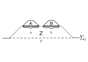
Figure 2: The horizontal line $\Sigma_{i}$ is the initial Cauchy surface. The dashed portion of $\Sigma_{i}$ represents $d:=\partial^{-}Z\cap\Sigma_{i}$. The future boundary of $Z$ can be partitioned into 3 sets: $a:=\partial^{-}A\cap\partial^{+}Z$, $b:=\partial^{-}B\cap\partial^{+}Z$ and the complement $c:=\partial^{+}Z\setminus(a\cup b)$. $a$ and $b$ are shown as bold lines and $c$ is indicated by the dotted line.

The delta function for the fields on $\partial^{+}Z$ is therefore a product of 3 delta functions for the field on $a$, $b$ and $c$:

$$\delta\left[\gamma|_{\partial^{+}Z}-\bar{\gamma}|_{\partial^{+}Z}\right]=\delta\left[\gamma|_{a}-\bar{\gamma}|_{a}\right]\,\,\delta\left[\gamma|_{b}-\bar{\gamma}|_{b}\right]\,\,\delta\left[\gamma|_{c}-\bar{\gamma}|_{c}\right]\,.$$ (50)

Now consider

$$D(E_{A}E_{\gamma_{Z}},\bar{E}_{A}E_{\bar{\gamma}_{Z}})$$ (51)

$$=\int_{\begin{subarray}{c}\Phi\in E_{A},\bar{\Phi}\in\bar{E}_{A}\\ \Phi|_{Z}=\gamma,\bar{\Phi}|_{Z}=\bar{\gamma}\end{subarray}}{\cal{D}}\Phi{\cal{D}}\bar{\Phi}\,\psi\left[\gamma|_{d}\right]^{*}\,\psi\left[\bar{\gamma}|_{d}\right]\,\,e^{-iS\left[\Phi\right]+iS\left[\bar{\Phi}\right]}\,\delta\left[\Phi|_{\partial^{+}(Z+A)}-\bar{\Phi}|_{\partial^{+}(Z+A)}\right]$$ (52)

$$=\psi\left[\gamma|_{d}\right]^{*}\,\psi\left[\bar{\gamma}|_{d}\right]\,\,e^{-iS\left[\gamma\right]+iS\left[\bar{\gamma}\right]}\delta\left[\gamma|_{c}-\bar{\gamma}|_{c}\right]\delta\left[\gamma|_{b}-\bar{\gamma}|_{b}\right]$$ (53)

$$\quad\quad\quad\quad\quad\quad\quad\int_{\Phi\in E_{A},\bar{\Phi}\in\bar{E}_{A}}{\cal{D}}\Phi{\cal{D}}\bar{\Phi}\,\,e^{-iS\left[\Phi|_{A}\right]+iS\left[\bar{\Phi}|_{A}\right]}\delta\left[\Phi|_{\partial^{+}A}-\bar{\Phi}|_{\partial^{+}A}\right]\,,$$ (54)

where the path integrals in the last line are over field configurations on region $A$ only.

Similarly,

$$D(E_{B}E_{\gamma_{Z}},\bar{E}_{B}E_{\bar{\gamma}_{Z}})$$ (55)

$$=\psi\left[\gamma|_{d}\right]^{*}\,\psi\left[\bar{\gamma}|_{d}\right]\,\,e^{-iS\left[\gamma\right]+iS\left[\bar{\gamma}\right]}\delta\left[\gamma|_{c}-\bar{\gamma}|_{c}\right]\delta\left[\gamma|_{a}-\bar{\gamma}|_{a}\right]$$ (56)

$$\quad\quad\quad\quad\quad\quad\quad\int_{\Phi\in E_{B},\bar{\Phi}\in\bar{E}_{B}}{\cal{D}}\Phi{\cal{D}}\bar{\Phi}\,\,e^{-iS\left[\Phi|_{B}\right]+iS\left[\bar{\Phi}|_{B}\right]}\delta\left[\Phi|_{\partial^{+}B}-\bar{\Phi}|_{\partial^{+}B}\right]\,,$$ (57)

and the path integrals are over field configurations on region $B$ only.

Finally,

$$D(E_{A}E_{B}E_{\gamma_{Z}},\bar{E}_{A}\bar{E}_{B}E_{\bar{\gamma}_{Z}})$$

$$=\psi\left[\gamma|_{d}\right]^{*}\,\psi\left[\bar{\gamma}|_{d}\right]\,\,e^{-iS\left[\gamma\right]+iS\left[\bar{\gamma}\right]}\delta\left[\gamma|_{c}-\bar{\gamma}|_{c}\right]$$

$$\quad\quad\int_{\Phi\in E_{A}E_{B},\bar{\Phi}\in\bar{E}_{A}\bar{E}_{B}}{\cal{D}}\Phi{\cal{D}}\bar{\Phi}\,\,e^{-iS\left[\Phi|_{A}\right]+iS\left[\bar{\Phi}|_{A}\right]}e^{-iS\left[\Phi|_{B}\right]+iS\left[\bar{\Phi}|_{B}\right]}$$ (58)

$$\quad\quad\quad\delta\left[\Phi|_{\partial^{+}A}-\bar{\Phi}|_{\partial^{+}A}\right]\delta\left[\Phi|_{\partial^{+}B}-\bar{\Phi}|_{\partial^{+}B}\right]\,.$$

The regions $A$ and $B$ are disjoint, the integrand is a product of factors that depend only on the field in $A$ and factors that depend only on the field in $B$. So the double path integral in A factorizes into a double path integral over fields on $A$ and a double path integral over fields on $B$:

$$D(E_{A}E_{B}E_{\gamma_{Z}},\bar{E}_{A}\bar{E}_{B}E_{\bar{\gamma}_{Z}})$$ (59)

$$=\psi\left[\gamma|_{d}\right]^{*}\,\psi\left[\bar{\gamma}|_{d}\right]\,\,e^{-iS\left[\gamma\right]+iS\left[\bar{\gamma}\right]}\delta\left[\gamma|_{c}-\bar{\gamma}|_{c}\right]$$ (60)

$$\quad\quad\int_{\Phi\in E_{A},\bar{\Phi}\in\bar{E}_{A}}{\cal{D}}\Phi{\cal{D}}\bar{\Phi}\,\,e^{-iS\left[\Phi|_{A}\right]+iS\left[\bar{\Phi}|_{A}\right]}\,\,\delta\left[\Phi|_{\partial^{+}A}-\bar{\Phi}|_{\partial^{+}A}\right]$$ (61)

$$\quad\quad\int_{\Phi\in E_{B},\bar{\Phi}\in\bar{E}_{B}}{\cal{D}}\Phi{\cal{D}}\bar{\Phi}\,\,e^{-iS\left[\Phi|_{B}\right]+iS\left[\bar{\Phi}|_{B}\right]}\,\,\delta\left[\Phi|_{\partial^{+}B}-\bar{\Phi}|_{\partial^{+}B}\right]\,.$$ (62)

Putting this together, we see that the $\psi$ factors on the LHS and on the RHS of (48) are equal, as are the $e^{-iS\left[\gamma\right]+iS\left[\bar{\gamma}\right]}$ factors, as are the delta function factors for the $\gamma$ and $\bar{\gamma}$ histories on the future boundary of $Z$. We also see that the double path integral factors are equal on the LHS and on the RHS of (48). Hence the result.

∎

References

- [1] R.D. Sorkin, On the Role of Time in the Sum Over Histories Framework for Gravity, Int.J.Theor.Phys. 33 (1994) 523.
- [2] R.D. Sorkin, Quantum mechanics as quantum measure theory, Mod. Phys. Lett. A9 (1994) 3119 [gr-qc/9401003].
- [3] R.D. Sorkin, Quantum measure theory and its interpretation, in Quantum Classical Correspondence: Proceedings of 4th Drexel Symposium on Quantum Nonintegrability, September 8-11 1994, Philadelphia, PA, D. Feng and B.-L. Hu, eds., pp. 229–251, International Press, Cambridge, Mass., 1997 [gr-qc/9507057].
- [4] R.D. Sorkin, Quantum Dynamics without the Wave Function, J. Phys. A40 (2007) 3207 [quant-ph/0610204].
- [5] R.D. Sorkin, An Exercise in ‘anhomomorphic logic’, J.Phys.Conf.Ser. 67 (2007) 012018 [quant-ph/0703276].
- [6] R.D. Sorkin, Logic is to the quantum as geometry is to gravity, in Foundations of Space and Time: Reflections on Quantum Gravity, J.M. G.F.R. Ellis and A. Weltman, eds., Cambridge University Press (2012) [1004.1226].
- [7] J.B. Hartle, The quantum mechanics of cosmology, in Quantum Cosmology and Baby Universes: Proceedings of the 1989 Jerusalem Winter School for Theoretical Physics, S. Coleman, J.B. Hartle, T. Piran and S. Weinberg, eds., World Scientific, Singapore (1991).
- [8] J.B. Hartle, The space time approach to quantum mechanics, Vistas Astron. 37 (1993) 569 [gr-qc/9210004].
- [9] J.B. Hartle, Space-time quantum mechanics and the quantum mechanics of space-time, in Proceedings of the Les Houches Summer School on Gravitation and Quantizations, Les Houches, France, 6 Jul - 1 Aug 1992, J. Zinn-Justin and B. Julia, eds., North-Holland, 1995 [gr-qc/9304006].
- [10] J.B. Hartle, Generalizing quantum mechanics for quantum spacetime, in The Quantum Structure of Space and Time, pp. 21–43, World Scientific, Singapore (2007) [gr-qc/0602013].
- [11] A. Fine, Hidden variables, joint probability and the Bell inequalities, Phys. Rev. Lett. 48 (1982) 291.
- [12] X. Martin, D. O’Connor and R.D. Sorkin, The random walk in generalized quantum theory, Phys. Rev. D71 (2005) 024029 [gr-qc/0403085].
- [13] F. Dowker, S. Johnston and R.D. Sorkin, Hilbert Spaces from Path Integrals, J. Phys. A43 (2010) 275302 [1002.0589].
- [14] F. Dowker, S. Johnston and S. Surya, On extending the Quantum Measure, J.Phys.A A43 (2010) 505305 [1007.2725].
- [15] R.D. Sorkin, Toward a fundamental theorem of quantal measure theory, Mathematical Structures in Computer Science 22 (2012) 816.
- [16] S. Surya and S. Zalel, A criterion for covariance in complex sequential growth models, Classical and Quantum Gravity 37 (2020) 195030 [2003.11311].
- [17] S. Surya and S. Zalel, A Criterion for Covariance in Complex Sequential Growth Models, Class. Quant. Grav. 37 (2020) 195030 [2003.11311].
- [18] F. Dowker and H. Wilkes, An argument for strong positivity of the decoherence functional in the path integral approach to the foundations of quantum theory, AVS Quantum Science 4 (2022) 012601 [2011.06120].
- [19] J.J. Halliwell and P. Wallden, Invariant class operators in the decoherent histories analysis of timeless quantum theories, Phys. Rev. D 73 (2006) 024011.
- [20] J.F. Clauser, M.A. Horne, A. Shimony and R.A. Holt, Proposed experiment to test local hidden-variable theories, Phys. Rev. Lett. 23 (1969) 880.
- [21] F. Dowker, J. Henson and P. Wallden, A histories perspective on characterizing quantum non-locality, New J.Phys. 16 (2014) 033033 [1311.6287].
- [22] D.A. Craig, H.F. Dowker, J. Henson, M. S., D. Rideout and R.D. Sorkin, A Bell Inequality Analog in Quantum Measure Theory, J. Phys. A40 (2007) 501 [quant-ph/0605008].
- [23] M. Navascués, S. Pironio and A. Acín, A convergent hierarchy of semidefinite programs characterizing the set of quantum correlations, New Journal of Physics 10 (2008) 073013 [0803.4290].
- [24] M. Navascués, Y. Guryanova, M.J. Hoban and A. Acín, Almost quantum correlations, Nature Communications 6 (2015) .
- [25] A. Stairs, Quantum logic, realism, and value definiteness, Philosophy of Science 50 (1983) 578.
- [26] D.M. Greenberger, M.A. Horne and A. Zeilinger, Going Beyond Bell’s Theorem, in Bell’s Theorem, Quantum Theory, and Conceptions of the Universe, pp. 69–72, Kluwer, Dordrecht (1989) [0712.0921].
- [27] L. Hardy, Quantum mechanics, local realistic theories and Lorentz-invariant realistic theories, Phys. Rev. Lett. 68 (1992) 2981.
- [28] J. Bell, La nouvelle cuisine, in Between science and technology, pp. 216–233, Elsevier (1990).
- [29] T. Norsen, John S. Bell’s concept of local causality, American Journal of Physics 79 (2011) 1261 [https://doi.org/10.1119/1.3630940].
- [30] J. Butterfield, David Lewis Meets John Bell, Philosophy of Science 59 (1992) 26.
- [31] J. Butterfield, Outcome Dependence and Stochastic Einstein Nonlocality, in Logic and Philosophy of Science in Uppsala, (Selected Papers from the 9th International Congress of Logic Methodology and Philosophy of Science), pp. 385–424, Kluwer (1994).
- [32] A. Einstein in The Born-Einstein letters: Correspondence Between Albert Einstein and Max and Hedwig Born from 1916-1955, with Commentaries by Max Born. Trans: Irene Born, p. 158, MacMillan (1971).
- [33] A.N. Kolmogorov, Complete metric boolean algebras, Philosophical Studies: An International Journal for Philosophy in the Analytic Tradition 77 (1995) 57.
- [34] S. Sinha and R.D. Sorkin, A Sum over histories account of an EPR(B) experiment, Found.Phys.Lett. 4 (1991) 303.
- [35] S. Popescu and D. Rohrlich, Nonlocality as an axiom, Foundations of Physics 24 (1994) 379.
- [36] B. Cirel’son, Quantum generalizations of Bell’s inequality, Lett. Math. Phys 4 (1980) 93.
- [37] B. Tsirel’son, Quantum analogues of the Bell inequalities. the case of two spatially separated domains, J. Soviet Math. 36 (1987) 557.
- [38] R.B. Griffiths, Consistent histories and the interpretation of quantum mechanics, J. Statist. Phys. 36 (1984) 219.
- [39] R. Omnès, Logical reformulation of quantum mechanics. 1. Foundations, J. Stat. Phys. 53 (1988) 893.
- [40] M. Gell-Mann and J.B. Hartle, Quantum mechanics in the light of quantum cosmology, in Complexity, Entropy and the Physics of Information, SFI Studies in the Sciences of Complexity, Vol VIII, W. Zurek, ed., pp. 150–173, Addison Wesley, Reading, 1990.
- [41] H.F. Dowker and R.D. Sorkin, Spin and statistics in quantum gravity, AIP Conference Proceedings 545 (2000) 205 [gr-qc/0101042].