Graph Neural Convection-Diffusion with Heterophily

Abstract

Graph neural networks (GNNs) have shown promising results across various graph learning tasks, but they often assume homophily, which can result in poor performance on heterophilic graphs. The connected nodes are likely to be from different classes or have dissimilar features on heterophilic graphs. In this paper, we propose a novel GNN that incorporates the principle of heterophily by modeling the flow of information on nodes using the convection-diffusion equation (CDE). This allows the CDE to take into account both the diffusion of information due to homophily and the “convection” of information due to heterophily. We conduct extensive experiments, which suggest that our framework can achieve competitive performance on node classification tasks for heterophilic graphs, compared to the state-of-the-art methods. The code is available at https://github.com/zknus/Graph-Diffusion-CDE.

1 Introduction

Graph Neural Networks (GNNs) have gained popularity in analyzing complex, structured data collected from various domains including social networks, citation networks, and molecular biology Veličković et al. (2018); Ji et al. (2023); Kang et al. (2023). These datasets depict entities as nodes and relationships between entities as edges. Most pioneering GNN works like Kipf and Welling (2017); Veličković et al. (2018); Hamilton et al. (2017); Xu et al. (2019); Kipf and Welling (2016); Klicpera et al. (2019); Lee et al. (2022) assume the graph datasets have strong homophily, where linked nodes often belong to the same class or have similar features. These models fail to optimally utilize information in heterophilic graph datasets, where connected nodes are likely from distinct classes or possess dissimilar features. A study by Sun et al. (2022) concludes that even simple models that do not take into account the graph structure, such as multilayer perceptrons (MLPs), can surpass several existing GNN models on heterophilic datasets.

To tackle this challenge, several models like Pei et al. (2019); Zhu et al. (2020); Chien et al. (2021); Zhu et al. (2021); Bo et al. (2021); Yang et al. (2021); Luan et al. (2022); Bodnar et al. (2022); Chanpuriya and Musco (2022); Sun et al. (2022); Li et al. (2022); Ma et al. (2021); Wang et al. (2022); Du et al. (2022) have been proposed. These works propose various techniques, such as aggregating higher-order neighborhoods, preserving high-frequency input signals, and adopting feature propagation methods, to improve the representation power of GNNs on heterophilic graph datasets.

Recently, works such as Chamberlain et al. (2021a, b); Song et al. (2022) have incorporated Neural Partial Differential Equations (PDEs) into GNNs, utilizing a variety of diffusion models for message passing on graphs. In this paper, our focus is on specific diffusion-based graph PDE models to address graph heterophily, as opposed to more general graph PDEs like those presented in the study by Rusch et al. (2022). The latter models nodes in a graph as coupled oscillators and establishes a second-order Ordinary Differential Equation (ODE) for updating node features. In Chamberlain et al. (2021a), the authors model information propagation as a diffusion process of a substance from regions of higher to lower concentration, such as heat diffusion from a hot object to a cold surface. However, due to the nature of heat diffusion, the features of neighboring nodes tend to become increasingly smooth. In heterophilic graphs, where connected nodes are likely to have dissimilar features, this method of message passing may not be appropriate. The paper Bodnar et al. (2022) proposes more general sheaf diffusion operators to control the diffusion process and maintain the non-smoothness in heterophily graphs, resulting in improved node classification performance. Furthermore, the study Zhu et al. (2022) reveals a strong connection between heterophily and the robustness of GNNs. Recently, research has drawn inspiration from works like Kang et al. (2021); Song et al. (2021) to explore how specially designed diffusion processes could enhance the robustness of GNNs against adversarial attacks. This has been demonstrated in the context of both classification Song et al. (2022) and localization tasks Wang et al. (2023a). Further research on diffusion models for heterophilic graphs is of particular interest.

In this paper, we propose a novel GNN inspired by the convection-diffusion process. Our proposed model explicitly incorporates the principle of heterophily in its design, which differentiates it from existing graph neural diffusion models. In a convection-diffusion heat transfer process in a fluid or gas, heat is not only transferred through diffusion due to heat concentration gradients but also through the movement of the fluid or gas itself. The velocity term in convection can be thought of as the movement of heat energy from one place to another due to the physical movement of a fluid or gas. The curvature-preserving diffusion models such as Beltrami and mean-curvature Chamberlain et al. (2021b); Song et al. (2022) are able to slow down the diffusion at the nodes where the feature difference between neighboring nodes is large, thereby preserving the non-smoothness and network robustness. Our model generalizes these curvature-preserving models by introducing a convection term in the diffusion equation that explicitly controls the propagation velocity at each node.

Main contributions. In this paper, our objective is to develop a general diffusion-based graph PDE framework that is suitable for heterophilic graph datasets. Our main contributions are summarized as follows:

1. Based on the convection-diffusion equation (CDE), we propose a graph neural convection-diffusion model that includes both a diffusion and convection term. The diffusion term aggregates information from homophilic neighbors, while the convection term allows controlled information propagation from heterophilic neighbors.

2. To manage the convection term in our CDE model, we introduce a learnable mechanism that adjusts the propagation rate at every node, allowing for better handling of heterophily.

3. We conduct extensive experiments on benchmark heterophilic datasets and compare with state-of-the-art baselines. Our experiments demonstrate that our model is competitive compared to the baselines, especially on large and more heterophilic datasets.

2 Related Work

In what follows, we briefly review the GNNs that are proposed to handle heterophilic graphs and recent advances in graph neural diffusion models.

2.1 Graph Neural Networks with Heterophily

Several works aim to adapt normal GNNs to heterophilic networks. H2GCN Zhu et al. (2020) proposes three effective designs to boost the performance of GNNs on heterophilic graphs, including the ego- and neighbor-embedding separation, higher-order neighborhood aggregation, and the combination of intermediate representations. Geom-GCN Pei et al. (2019) maps the graph to a suitable latent space where it can aggregate immediate neighborhoods and distant nodes to preserve the topology patterns of the graph. GPR-GNN Chien et al. (2021) assigns each step of feature propagation with a learnable weight, which can be negative or positive, to mitigate graph heterophily and over-smoothing issues. CPGNN Zhu et al. (2021) incorporates a compatibility matrix into GNNs to learn the likelihood of connections between nodes in different classes, which allows a GNN to capture both heterophily and homophily patterns in the graph. FAGCN Bo et al. (2021) integrates the low-frequency signals, high-frequency signals, and raw features adaptively through a self-gating mechanism to enhance the expressive power of GNNs on disassortative networks. ACM-GCN Luan et al. (2022) adaptively learns the local and node-wise information through aggregation, diversification, and identity channels. In this way, it can retain the low-frequency and high-frequency components of the input signal. Instead of using fixed feature propagation step in SGC Wu et al. (2019), ASGC Chanpuriya and Musco (2022) applies a learned polynomial of the normalized adjacency matrix with the input feature to fit a different filter for each feature. Our work is different from these previous works as we mainly focus on the use of graph PDEs to model the information propagation in heterophilic graphs.

2.2 Graph Neural Diffusion

In this subsection, we provide a brief overview of various graph neural diffusion models that have been proposed recently. In Chamberlain et al. (2021a), the authors modeled information propagation as a diffusion process of a substance from regions of higher to lower concentration. The Beltrami diffusion model was utilized in Chamberlain et al. (2021b); Song et al. (2022) to enhance rewiring and improve the robustness of the graph. The above works do not specifically target the problem of graph heterophily.

To address diffusion in heterophilic graphs, the paper Bodnar et al. (2022) introduces general sheaf diffusion operators to control the diffusion process and maintain non-smoothness in heterophilic graphs, leading to improved node classification performance. Inspired by the particle reaction-diffusion process, the ACMPWang et al. (2023b) models the heterophilic graph by employing both repulsive and attractive force interactions as dual flow directions between nodes. Our approach differs from the aforementioned diffusion models in that we incorporate a convection term that is able to adapt to the complex connections in heterophilic graphs.

3 Preliminaries

In this section, we first introduce the convection-diffusion equation (CDE). We then review graph neural diffusion formulations that are used in our graph CDE model and will be later used in experiments on graph datasets.

3.1 Convection-Diffusion Equation

In Chamberlain et al. (2021a), the authors unified many popular GNN architectures into a single mathematical framework that is derived from the following (heat) diffusion equation. Let $x(u,t)$ denote a scalar-valued function on $\Omega\times[0,\infty)$, e.g., $x(u,t)$ can be the temperature at point $u$ on the space $\Omega$ at time $t$. The heat diffusion Grigoryan (2009) process is formulated as

$$\frac{\partial x}{\partial t}=\operatorname{div}(D\nabla x),\ t>0,$$ (1)

with some initial boundary condition that specifies the temperature distribution at $t=0$, and $\operatorname{div}$ and $\nabla$ are the divergence and concentration gradient operators, respectively. Here $D$ is the thermal diffusivity for heat diffusion, which may vary at different positions in an inhomogeneous material and leads to position-dependent diffusion directions and speeds. In the GNN models Song et al. (2022); Chamberlain et al. (2021a), the authors design different formulations $D$ to model the information propagation between graph nodes that may depend on the node and its neighbors.

The CDE, on the other hand, describes physical phenomena such as heat transfer within a physical system, resulting from the combination of two processes: diffusion and convection. The CDE is given by

$$\frac{\partial x}{\partial t}=\operatorname{div}(D\nabla x)-\operatorname{div}(\mathbf{v}x)$$ (2)

where the first term represents the heat diffusion, same as in 1, and the second term $\operatorname{div}(\mathbf{v}x)$ in the equation represents the convection process. The velocity field $\mathbf{v}$ is a function of both time and space and describes how the quantity is moving. In oceanography, the convection-diffusion equation is used to model the transfer of heat in the ocean. The variable $x$ would represent the concentration of heat in the ocean, and the velocity field $\mathbf{v}$ would represent the ocean currents and water flow as a function of both time and location.

3.2 Common Graph Neural Diffusion Models

Suppose $\mathcal{G}=(\mathcal{V},\mathcal{E},w)$ is a graph, where $\mathcal{V}=\{1,\dots,N\}$ is the set of $N$ nodes, $\mathcal{E}\subseteq\mathcal{V}\times\mathcal{V}$ is the set of edges, and $w:\mathcal{E}\rightarrow\mathbb{R}^{+}$ the edge weight function. The features for the vertices at time $t$ are represented by $\mathbf{X}(t)\in\mathbb{R}^{|\mathcal{V}|\times r}$ where $r$ is the node feature dimension. The $i$-th row of $\mathbf{X}(t)$, denoted as $\mathbf{x}^{\intercal}_{i}(t)$, is the feature vector for vertex $i$ at time $t$.

In the literature, several graph diffusion models Chamberlain et al. (2021a); Song et al. (2022); Bodnar et al. (2022) have been proposed, which are mostly derived from the heat equation 1 with different diffusivities $D$ learned from the graph datasets. For example, inspired from the heat diffusion equation 1, GRAND Chamberlain et al. (2021a) defines the following graph version of the gradient $\nabla$ and divergence $\operatorname{div}$ operators as

$$(\nabla\mathbf{X}(t))_{(i,j)}=\mathbf{x}_{j}(t)-\mathbf{x}_{i}(t),\ \forall\,(i,j)\in\mathcal{E}$$ (3)

for each edge $(i,j)\in\mathcal{E}$ in the graph, and

$$(\operatorname{div}(\mathscr{X}))_{i}=\sum_{j:(i,j)\in\mathcal{E}}\mathscr{X}_{ij},$$ (4)

where $\mathscr{X}=\{\mathscr{X}_{ij}\}_{(i,j)\in\mathcal{E}}$ is the set of all features associated with edges and $\mathscr{X}_{ij}\in\mathbb{R}^{r}$ is the feature associated with edge $(i,j)$. Furthermore, for graph learning, they implement the following dynamical system:

$$\frac{{\partial}\mathbf{X}(t)}{{\partial}t} =\operatorname{div}(D(\mathbf{X}(t),t)\odot\nabla\mathbf{X}(t))$$

$$=(\mathbf{A}(\mathbf{X}(t))-\mathbf{I})\mathbf{X}(t)$$ (5)

where the initial condition is given by $\mathbf{X}(0)=\left(\mathbf{x}^{{}^{\intercal}}_{0}(0),\cdots,\mathbf{x}^{{}^{\intercal}}_{|\mathcal{V}|}(0)\right)^{{}^{\intercal}}$, $\odot$ is the element-wise product and the diffusivity $D$ is a $|\mathcal{E}|\times|\mathcal{E}|$ diagonal matrix with elements $\operatorname{diag}(a(\mathbf{x}_{i}(t),\mathbf{x}_{j}(t),t))$. Here, $a(\cdot)$ is a similarity function for vertex pairs. The diffusion equation can therefore be reformed as 5 with matrix $\mathbf{A}(\mathbf{X}(t))=\left(a\left(\mathbf{x}_{i}(t),\mathbf{x}_{j}(t)\right)\right)$, which is a learnable attention matrix used to describe the structure of the graph, and $\mathbf{I}$ being an identity matrix.

We refer the readers to the supplementary material for more details about other diffusion variants like the graph Beltrami flow Song et al. (2022), and graph sheaf diffusion Bodnar et al. (2022).

3.3 Graph Heterophily

In this section, we introduce the graph homophily measure, which is used in the experiments in Section 5 to quantify the homophily level of a graph dataset.

Definition 1 (Edge homophily ratio Zhu et al. (2020)).

The edge homophily ratio is defined as:

$$h_{\mathrm{edge}}=\frac{|\left\{(u,v)\nonscript\,:\allowbreak\nonscript\,\mathopen{}(u,v)\in\mathcal{E}\wedge y_{u}=y_{v}\right\}|}{|\mathcal{E}|}.$$ (6)

This ratio is the proportion of edges in a graph that connects nodes with the same class label (i.e., intra-class edges). A smaller $h_{\mathrm{edge}}$ implies stronger heterophily.

The edge homophily ratio is sensitive to the number of classes and the balance of classes in a graph. To fairly compare the homophily ratio across different datasets with different numbers of classes and class balance, the paper Platonov et al. (2022) proposes the adjusted homophily ratio as follows.

Definition 2 (Adjusted homophily ratio Platonov et al. (2022)).

Suppose there are $C$ classes. The adjusted homophily ratio is given by

$$h_{\mathrm{adj}}=\frac{h_{\mathrm{edge}}-\sum_{k=1}^{C}D_{k}^{2}/(2|\mathcal{E}|)^{2}}{1-\sum_{k=1}^{C}D_{k}^{2}/(2|\mathcal{E}|)^{2}}$$ (7)

where $D_{k}:=\sum_{i:y_{i}=k}d(i)$, $y_{i}$ is the label of node $i$, and $d(i)$ is the degree of node $i$.

4 Graph Neural Convection-Diffusion

We now consider graph neural convection-diffusion by making use of concepts from Section 3. In homophilic graphs, the edges between nodes tend to be between similar nodes, analogous to homogeneous atoms or molecules in a solid material. In such materials, these connections are relatively stable. The movement of atoms or molecules is relatively limited by the strength of the connections between them, and the heat transfer is mainly described using 1. Analogously, the information aggregation in homophilic graphs can be well-described by the graph heat diffusion equation Chamberlain et al. (2021c).

In contrast, heterophilic graphs have connections between dissimilar nodes, analogous to having different types of particles in a gas or fluid. These connections are less stable, and the movement of particles is relatively unrestricted. This makes heterophilic graphs well-suited to be regarded as soft materials, where the movement of particles is not limited by the strength of their connections. In the CDE 2, the velocity term (convection) is used to model the movement of the fluid or gas itself. For information propagation in heterophilic graphs, the convection term can help us to assign different information propagation velocities to each node due to the different connections.

The graph analogy of 2 can be formulated as

$$\frac{\partial}{\partial t}\mathbf{X}(t)=\operatorname{div}(D(\mathbf{X}(t),t)\odot\nabla\mathbf{X}(t))+\operatorname{div}(\mathbf{V}(t)\circ\mathbf{X}(t))$$ (8)

where the first diffusion term $\operatorname{div}(D(\mathbf{X}(t),t)\odot\nabla\mathbf{X}(t))$ could be given by 5 or other variants in Song et al. (2022); Bodnar et al. (2022), $\mathbf{V}_{ij}(t)\in\mathbb{R}^{r}$ is the velocity vector associated with each edge $(i,j)$ at time $t$, $\mathbf{V}(t)=\{\mathbf{V}_{ij}(t)\}_{(i,j)\in\mathcal{E}}$, and

$$(\operatorname{div}(\mathbf{V}(t)\circ\mathbf{X}(t)))_{i}\coloneqq\sum_{j:(i,j)\in\mathcal{E}}\mathbf{V}_{ij}(t)\odot\mathbf{x}_{j}(t)$$ (9)

for each node $i\in\mathcal{V}$.

4.1 $\mathbf{V}_{ij}$ for Heterophily

We propose the following simple yet effective velocity formulation:

$$\mathbf{V}_{ij}=\sigma\left(W(\mathbf{x}_{j}(t)-\mathbf{x}_{i}(t))\right),$$ (10)

where $W$ is a learnable matrix and $\sigma$ denotes an activation function. In 10, the velocity $\mathbf{V}_{ij}$ determines the direction of preferred information transport from node $j$ to its neighboring node $i$. The velocity is determined by the difference $\mathbf{x}_{j}(t)-\mathbf{x}_{i}(t)$ of the feature representations of the neighboring nodes. Note that the velocity is not always in the same direction as the difference $\mathbf{x}_{j}(t)-\mathbf{x}_{i}(t)$ due to the learnable $W$ and activation function. The use of the velocity term in the dot product with the state of the neighboring node in 9 allows for a more flexible and adaptive information flow for heterophilic graphs. This is because it takes into account the dissimilarity of neighboring nodes, which is a unique characteristic of heterophilic graphs. In contrast, traditional neural PDEs Chamberlain et al. (2021a); Song et al. (2022) utilize only a single diffusion process, which does not consider the dissimilarity of neighboring nodes. The addition of the convection term in the CDE allows for a more accurate representation of the information flow in heterophilic graphs. For a more comprehensive understanding of our model, we direct readers to the supplementary material.

4.2 Model Details

We present our algorithm in Algorithm 1. Our approach is based the graph neural PDE defined in 8. This graph PDE is distinct from the diffusion-based models presented in previous works such as Chamberlain et al. (2021a); Song et al. (2022); Bodnar et al. (2022). To solve the neural PDE, we follow the convention in these previous works and use the provided solver from Chen et al. (2018). Our main contribution is the introduction of the second term in 8, which utilizes a simple yet effective velocity formulation 10). The first term in 8 has various options as discussed in Song et al. (2022); Chamberlain et al. (2021c).

Algorithm 1 Neural CDE Inference

1:$\mathcal{G}=(\mathcal{V},\mathcal{E})$, integration time $T$.

2:Graph task results

3:Compress the sparse raw input node feature using an MLP and set them as the initial conditions $\{\mathbf{x}_{i}(0)\}_{i=1}^{|\mathcal{V}|}$.

4:Solve the neural PDE 8 using explicit or implicit solvers fromChen et al. (2018).

5:Return $\{\mathbf{x}_{i}(T)\}_{i=1}^{|\mathcal{V}|}$ which is the solution of 8 at time $T$.

6:Perform further graph tasks, e.g., node classification.

5 Experiments

Dataset	Nodes	Edges	Classes	Node Features	Edge homophily $h_{\mathrm{edge}}$	Adjusted homophily $h_{\mathrm{adj}}$
Roman-empire	22662	32927	18	300	0.05	-0.05
Wiki-cooc	10000	2243042	5	100	0.34	-0.03
Minesweeper	10000	39402	2	7	0.68	0.01
Questions	48921	153540	2	301	0.84	0.02
Workers	11758	519000	2	10	0.59	0.09
Amaon-ratings	24492	93050	5	300	0.38	0.14
Texas	183	295	5	1703	0.11	0.04
Cornel	183	280	5	1703	0.30	0.04
Wisconsin	251	466	5	1703	0.21	0.07

Table 1: Bechmark’s statistics

Method	Roman-empire	Wiki-cooc	Minesweeper	Questions	Workers	Amazon-ratings	Texas	Cornell	Wisconsin
$h_{\mathrm{adj}}$	-0.05	-0.03	0.01	0.02	0.09	0.14	0.04	0.04	0.07
ResNet	65.71$\pm$0.44	89.36$\pm$0.71	50.95$\pm$1.12	70.10$\pm$0.75	73.08$\pm$1.28	45.70$\pm$0.69	80.81$\pm$4.75	81.89$\pm$6.40	85.29$\pm$3.31
GCN	70.51$\pm$0.75	91.01$\pm$0.69	89.47$\pm$0.69	75.97$\pm$1.23	83.14$\pm$1.11	47.77$\pm$0.69	55.14$\pm$5.16	60.54$\pm$5.30	51.76$\pm$3.06
GraphSAGE	85.80$\pm$0.69	93.60$\pm$0.31	93.53$\pm$0.50	76.52$\pm$0.93	82.34$\pm$0.19	52.77$\pm$0.54	82.43$\pm$6.14	75.95$\pm$5.01	81.18$\pm$5.56
GAT	81.02$\pm$0.46	92.44$\pm$0.80	92.10$\pm$0.67	77.42$\pm$1.23	83.98$\pm$0.57	47.95$\pm$0.53	52.16$\pm$6.63	61.89$\pm$5.05	49.41$\pm$4.09
H2GCN	68.09$\pm$0.29	89.24$\pm$0.32	89.95$\pm$0.38	66.66$\pm$1.84	81.76$\pm$0.68	41.36$\pm$0.47	84.86$\pm$7.23	82.70$\pm$5.28	87.65$\pm$4.98
CPGNN	63.78$\pm$0.50	84.84$\pm$0.66	71.27$\pm$1.14	67.09$\pm$2.63	72.44$\pm$0.80	44.36$\pm$0.35	75.68$\pm$5.12	70.27$\pm$5.12	76.47$\pm$6.16
GPR-GNN	73.37$\pm$0.68	91.90$\pm$0.78	81.79$\pm$0.98	73.41$\pm$1.24	70.59$\pm$1.15	43.90$\pm$0.48	81.35$\pm$5.32	78.11$\pm$6.55	82.55$\pm$6.23
GloGNN	63.85$\pm$0.49	88.49$\pm$0.45	62.53$\pm$1.34	67.15$\pm$1.92	73.90$\pm$0.95	37.28$\pm$0.66	84.32$\pm$4.15	83.51$\pm$4.26	87.06$\pm$3.53
FAGCN	70.53$\pm$0.99	91.88$\pm$0.37	89.69$\pm$0.60	77.04$\pm$1.56	81.87$\pm$0.94	46.32$\pm$2.50	82.43$\pm$6.89	79.19$\pm$9.79	82.94$\pm$7.95
GBK-GNN	75.87$\pm$0.43	97.81$\pm$0.32	83.56$\pm$0.84	72.98$\pm$1.05	78.06$\pm$0.91	43.47$\pm$0.51	81.08$\pm$4.88	74.27$\pm$2.18	84.21$\pm$4.33
ACM-GCN	68.35$\pm$1.95	87.48$\pm$1.06	90.47$\pm$0.57	OOM	78.25$\pm$0.78	38.51$\pm$3.38	87.84$\pm$4.40	85.14$\pm$6.07	88.43$\pm$3.22
GRAND	71.60$\pm$0.58	92.03$\pm$0.46	76.67$\pm$0.98	70.67$\pm$1.28	75.33$\pm$0.84	45.05$\pm$0.65	80.27$\pm$4.84	82.97$\pm$6.63	83.73$\pm$3.51
GraphBel	69.47$\pm$0.37	90.30$\pm$0.50	76.51$\pm$1.03	70.79$\pm$0.99	73.02$\pm$0.92	43.63$\pm$0.42	80.27$\pm$3.64	83.51$\pm$6.45	85.29$\pm$4.82
Diag-NSD	77.50$\pm$0.67	92.06$\pm$0.40	89.59$\pm$0.61	69.25$\pm$1.15	79.81$\pm$0.99	37.96$\pm$0.20	85.67$\pm$6.95	86.49$\pm$7.35	88.63$\pm$2.75
ACMP	71.27$\pm$0.59	92.68$\pm$0.37	76.15$\pm$1.12	71.18$\pm$1.03	75.03$\pm$0.92	44.76$\pm$0.52	86.20$\pm$3.0	85.40$\pm$7.0	86.10$\pm$4.0
CDE-GRAND	91.64$\pm$0.28	97.99$\pm$0.38	95.50$\pm$5.23	75.17$\pm$0.99	80.70$\pm$1.04	47.63$\pm$0.43	86.22$\pm$3.30	86.22$\pm$5.05	87.45$\pm$4.40
CDE-GraphBel	85.39$\pm$0.46	97.79$\pm$0.40	93.98$\pm$0.57	72.11$\pm$1.31	81.30$\pm$0.43	45.22$\pm$0.60	87.57$\pm$3.24	85.14$\pm$5.95	87.84$\pm$4.87

Table 2: Node classification results(%). The best and the second-best result for each criterion are highlighted in bold and underlined respectively. The results are accuracy on Wiki-cooc, Roman-empire, Amaon-ratings, Texas, Cornell and Wisconsin datasets and ROC-AUC score on Minesweeper, Workers, and Questions datasets. OOM refers to out-of-memory on NVIDIA RTX A5000 GPU.

5.1 Real-World Datasets

The paper Pei et al. (2019) evaluates the performance of their model on six heterophilic graph datasets: Squirrel, Chameleon, Actor, Texas, Cornell, and Wisconsin. These are widely-used heterophilic benchmarks, and we also use them to evaluate different models’ node classification performance.

However, a recent paper Platonov et al. (2023) has pointed out a train-test data leakage problem in the Squirrel and Chameleon datasets collected by Rozemberczki et al. (2021), leading to questions on model performance on these two datasets. The datasets Cornell, Texas, and Wisconsin do not have this data leakage issue but are relatively small and have significantly imbalanced classes, which can result in overfitting for diffusion models Bodnar et al. (2022). We report the node classification results based on these three datasets in Table 2, where we use a fixed data splitting method as introduced in Pei et al. (2019). The experiments where we apply random data splitting are provided in the Appendix, where we also include experiments using Squirrel, Chameleon, and Actor datasets.

To fairly evaluate the model performance on heterophilic graph datasets, we additionally include six new heterophilic datasets proposed in Platonov et al. (2023). The proposed datasets come from different domains, such as English Wikipedia, the Amazon product co-purchasing network, and a question-answering platform. All of them have low homophily scores as verified in Platonov et al. (2023) and diverse structural properties. Platonov et al. (2023) evaluates a wide range of GNNs, both standard, and heterophily-specific, on these datasets and argues that the progress in graph learning under heterophily is limited since the standard baselines usually outperform heterophily-specific models on the datasets. For these heterophilic datasets, we follow the data splitting in Platonov et al. (2023), which is 50%, 25%, and 25% for training, validation, and testing. The data statistics are shown in Table 1. We use the ROC-AUC score as the evaluation metric on Minesweeper, Workers, and Questions datasets because they have binary classes. We include the synthetic regular graphs using the algorithm described in Luan et al. (2022) to control dataset heterophily for further demonstration.

5.2 Implementation and Baselines

We evaluate our neural CDE model on the node classification task against a variety of baseline models, including a graph-agnostic model, ResNet He et al. (2016), as well as standard GNN models such as GCN Kipf and Welling (2017), GAT Veličković et al. (2018), and GraphSAGE Hamilton et al. (2017). Additionally, we compare our model to GNNs specifically designed for heterophilic graphs, including H2GCN Zhu et al. (2020), CPGNN Zhu et al. (2021), GPR-GNN Chien et al. (2021), GloGNN Li et al. (2022), FAGCN Bo et al. (2021), GBK-GNN Du et al. (2022), and ACM-GCNLuan et al. (2022). We also include diffusion-based graph PDE models such as GRAND Chamberlain et al. (2021c), GraphBel Song et al. (2022), Diag-NSD Bodnar et al. (2022) and ACMP Wang et al. (2023b) as baselines.

We have implemented our CDE models using the algorithm outlined in Algorithm 1. In this model, the first diffusion term in 8 is specified by the graph diffusion formulation presented in previous works such as GRAND and GraphBel Chamberlain et al. (2021a); Song et al. (2022). We provide detailed descriptions of the specific diffusion formulations used in our implementation in Section 5.6.3. Specifically, we refer to our CDE model that utilizes the diffusion formulation in 12 as CDE-GRAND-GAT. For simplicity, we may use the abbreviation CDE-GRAND to refer to it in the rest of the paper. CDE-GraphBel refers to the CDE model with GraphBel being the first term. For all these datasets, we use the Adam optimizer Kingma and Ba (2014) with a learning rate of 0.01 and weight decay of 0.001. We also apply a dropout rate of 0.2 to prevent overfitting issues. We solve the neural PDE through the methods in Chen et al. (2018). The integration time and step size are adjusted according to the performance of validation data. For the Texas, Cornell, and Wisconsin datasets, which have much smaller sizes, we conduct the hyperparameter search on each dataset. We report the best hyperparameters of each dataset in the supplementary material.

5.3 Node Classification Results on Real-World Datasets

From Table 2, we observe that if we augment diffusion models like GRAND and GraphBel with our proposed CDE convection term 9, we can significantly improve the diffusion model performance on the heterophilic graph datasets. For example, on the Roman-empire dataset, CDE-GRAND improves GRAND’s performance from 71.60$\pm$0.58% to 91.64$\pm$0.28%. Similar improvements can be observed on all of the nine heterophilic graph datasets, demonstrating the effectiveness of our convection term in addressing the unique challenges of heterophilic graphs. This is because our velocity takes into account the dissimilarity of neighboring nodes in heterophilic graphs. For information propagation in heterophilic graphs, the convection term that includes the dot product between the neighboring node and the velocity helps us to assign flexible and adaptive information propagation flows to each node due to the different connections. We refer the readers to Section 5.6.3 for further demonstration.

Compared with all the baselines on heterophilic graph datasets, CDE-GRAND achieves the best performance on Wiki-cooc, Roman-empire, and Minesweeper. From Table 1, we observe that these datasets have the lowest adjusted homophily $h_{\mathrm{adj}}$, indicating they are highly heterophilic. Our results suggest that CDE diffusion is particularly effective on more heterophilic datasets. On the Roman-empire dataset, CDE-GRAND outperforms the second-best model, GraphSAGE, by a significant margin of 5.84%. Notably, GraphSAGE is a standard GNN that is not specifically designed for heterophilic graphs, yet it performs better than all heterophily-specific baselines, highlighting the current limitations in graph learning under heterophily Platonov et al. (2023). However, our CDE-GRAND model successfully surpasses GraphSAGE on this heterophilic dataset. A similar trend can be observed in the Minesweeper dataset where GraphSAGE achieves 93.53$\pm$0.50% and outperforms all the heterophily-specific baselines. Our CDE-GRAND model, however, can surpass GraphSAGE by a significant margin of 4.14%. On all other heterophilic graph datasets, CDE-GRAND performs comparably to state-of-the-art baselines, with the exception of Amazon-ratings, where all heterophily-specific models perform worse than GraphSAGE. This may be because the Amazon-ratings dataset has less heterophilic structure, as indicated by the largest adjusted homophily $h_{\mathrm{adj}}$ score presented in Table 1. As observed in Platonov et al. (2023) and Table 2, the modified GAT with residual connections outperforms all other heterophily-specific GNN models on the Questions, Workers, and Amazon-ratings datasets, hinting at unique geometries in these datasets that other models fail to capture effectively.

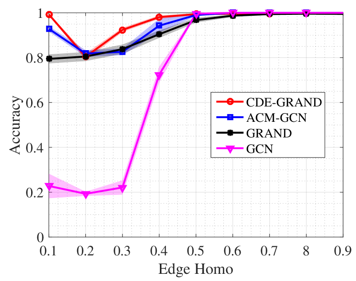
Figure 1: Accuracy versus edge homophily level. A node classification task based on the Cora dataset is used to compare different methods including CDE-GRAND, ACM-GCN, GRAND, and GCN.

5.4 Node Classification Results on Synthetic Datasets

We generate synthetic regular graphs using the algorithm described in Luan et al. (2022). The edge homophily levels range from 0.1 to 0.9, with 10 graphs generated for each level. Each graph contains 5 classes, with 400 nodes in each class. For each node, we randomly generate 10 edges to connect to nodes within the same class and [$\frac{10}{H_{\text{edge}}(\mathcal{G})}-10$] edges to nodes in other classes. The features of each node are sampled from the corresponding class of the base dataset, which is the Cora dataset in Fig. 1. The nodes are then randomly split into train, validation, and test sets at a ratio of 60%:20%:20%. The node classification results are displayed in Fig. 1.

From Fig. 1, we observe that CDE-GRAND outperforms other methods on classification accuracy. Especially when the edge homophily level is less than 0.5, the CDE-GRAND has advantages obviously. This indicates that our method is more adaptive to the heterophily of graphs than the other methods including ACM-GCN, GRAND, and GCN.

Time	ODE Solver	Roman-empire	Minesweeper
1.0	Euler Solver	87.26$\pm$0.46	87.13$\pm$1.36
	RK4 Solver	91.55$\pm$0.66	93.05$\pm$0.48
2.0	Euler Solver	91.55$\pm$0.42	90.46$\pm$0.66
	RK4 Solver	91.10$\pm$1.16	94.64$\pm$2.32
3.0	Euler Solver	91.64$\pm$0.28	92.00$\pm$0.60
	RK4 Solver	90.82$\pm$2.18	94.35$\pm$3.62
4.0	Euler Solver	91.62$\pm$0.34	93.21$\pm$0.43
	RK4 Solver	91.00$\pm$1.31	97.67$\pm$0.22
5.0	Euler Solver	91.16$\pm$0.67	93.11$\pm$2.36
	RK4 Solver	90.26$\pm$2.16	97.10$\pm$2.02

Table 3: Node classification accuracy under different integration times of CDE. The ODE solver is used with step size $\tau=1$. We fixed all other hyperparameters in the model except the integration time $T$. Unlike the traditional GNNs, the neural diffusion models do not have explicit layers but we may consider the steps taken to solve an ODE as the implicit layers. Hence, the number of implicit layers in neural diffusion models is $T/\tau$ for fixed step-size ODE solvers.

Method	Wiki-cooc	Roman-empire	Amazon-ratings	Minesweeper	Workers	Questions
GRAND-LAP	91.58$\pm$0.37	69.24$\pm$0.53	48.99$\pm$0.35	73.25$\pm$0.99	75.59$\pm$0.86	68.54$\pm$1.07
GRAND-GAT	92.03$\pm$0.46	71.60$\pm$0.58	45.05$\pm$0.65	76.67$\pm$0.98	75.33$\pm$0.84	70.67$\pm$1.28
GRAND-TRANS	91.86$\pm$0.27	71.18$\pm$0.56	45.20$\pm$0.52	75.40$\pm$1.36	75.13$\pm$0.65	69.14$\pm$0.97
GraphBel	90.30$\pm$0.50	69.47$\pm$0.37	43.63$\pm$0.42	76.51$\pm$1.03	73.02$\pm$0.92	70.79$\pm$0.99
CDE-GRAND-LAP	98.00$\pm$0.20	90.58$\pm$0.49	47.43$\pm$0.53	90.06$\pm$0.60	80.45$\pm$0.97	73.78$\pm$1.46
CDE-GRAND-GAT	97.99$\pm$0.38	91.64$\pm$0.28	47.63$\pm$0.43	95.50$\pm$5.23	80.70$\pm$1.04	75.17$\pm$0.99
CDE-GRAND-TRANS	98.04$\pm$0.35	91.55$\pm$0.23	46.91$\pm$0.87	91.38$\pm$1.92	81.58$\pm$0.98	72.92$\pm$1.54
CDE-GraphBel	97.79$\pm$0.40	85.39$\pm$0.46	45.22$\pm$0.60	90.79$\pm$0.48	81.30$\pm$0.43	72.11$\pm$1.31

Table 4: Node classification accuracy(%). We evaluate the performance of the vanilla diffusion variants and the inclusion of CDE convection.

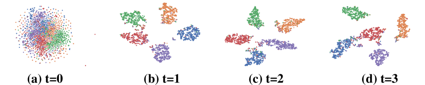
Figure 2: T-sne visualization of the feature representation from CDE-based neural diffusion models at different integration time $t$ on the synthetic dataset described in Section 5.4 . From left to right: $t=0$, $t=1$, $t=2$ and $t=3$

5.5 Visulization

The visualization of the node features from our CDE model at different integration time $t$ is shown in Fig. 2. From Fig. 2, we observe that the heterophilic graph dataset are classified into different classes by using our CDE models obviously.

5.6 Ablation Studies

5.6.1 Integration Time

We can see from Table 3 that as the integration time of our proposed CDE model increases, the node classification accuracy improves on the Roman-empire and Minesweeper datasets. However, there is a point at which the predicted classification results reach a saturation point. Therefore, it is important to consider the balance between accuracy and computation time when selecting the appropriate integration time for CDE, as a larger integration time results in increased computation time.

5.6.2 PDE Solvers

There are various numerical methods available for solving nonlinear diffusion equations. In this work, we primarily utilize explicit solvers provided in Chen et al. (2018) for our model. These solvers can be divided into single-step and multi-step schemes, where the latter involves the use of multiple function evaluations at different time steps to compute the next iteration. This results in multi-hop neighboring information aggregation in multi-step explicit solvers. In this work, we use a multi-step solver named RK4 and a single-step explicit solver named Euler. As seen in Table 3, RK4 outperforms Euler, particularly on the Minesweeper dataset. This is likely due to the higher-order neighborhood aggregation used in RK4, which has been shown to be effective for heterophilic graphs Zhu et al. (2020). However, the use of an RK4 solver typically results in higher computational complexity. In order to balance performance and computational efficiency, we choose to use the Euler solver for the experiments reported in Table 2, even though better performance may be achieved with the RK4 solver.

Method	Training Time (ms)	Inference Time (ms)
GRAND	9.55	4.66
GraphBel	12.55	6.69
CDE-GRAND	10.43	4.72
CDE-GraphBel	13.91	6.81

Table 5: Training time and inference time of models on the Cora dataset using Euler solver. Neural PDE models are based on the Euler solver with an integral time of 1.0 and a hidden dim of 64. The training and inference time refers to the average time for 100 rounds.

5.6.3 Diffusion Functions

In this section, we show the node classification performance under different diffusion functions compared to the vanilla diffusion variants defined in Chamberlain et al. (2021a); Song et al. (2022). The learnable attention matrix $\mathbf{A}(\mathbf{X}(t))=\left(a\left(\mathbf{x}_{i}(t),\mathbf{x}_{j}(t)\right)\right)$ in 5 can be formulated with three versions as used in Chamberlain et al. (2021a).

GRAND-TRANS uses the scaled dot product attention from the Transformer model Vaswani et al. (2017):

$$a(\mathbf{x}_{i},\mathbf{x}_{j})=\mathrm{softmax}\left(\frac{(\mathbf{W}_{K}\mathbf{x}_{i})^{\top}\mathbf{W}_{Q}\mathbf{x}_{j}}{d_{k}}\right),$$ (11)

where $\mathbf{W}_{K}$ and $\mathbf{W}_{Q}$ are learned matrices, and $d_{k}$ is a hyperparameter determining the dimension of $W_{k}$.

GRAND-GAT uses the attention in GAT model Veličković et al. (2018):

$$a(\mathbf{x}_{i},\mathbf{x}_{j})=\frac{\exp\left(\mathrm{LeakyReLU}\left(\mathbf{a}^{\intercal}\left[\mathbf{W}\mathbf{x}_{i}\|\mathbf{W}\mathbf{x}_{j}\right]\right)\right)}{\sum_{k\in\mathcal{N}_{i}}\exp\left(\mathrm{LeakyReLU}\left(\mathbf{a}^{\intercal}\left[\mathbf{W}\mathbf{x}_{i}\|W\mathbf{x}_{k}\right]\right)\right)},$$ (12)

where $\mathbf{W}$ and $\mathbf{a}$ are learned and $\|$ is the concatenation operator.

GRAND-LAP models the linear diffusion process, where the $\mathbf{A}(t)$ a constant in the integral, i.e., $\mathbf{A}(\mathbf{X}(t))=\mathbf{A}$ for a constant $\mathbf{A}$.

GraphBel is inspired by Beltrami diffusion Sochen et al. (1998). We refer readers to Song et al. (2022) for its diffusion formulation.

The results in table 4 show that our CDE framework significantly improves the node classification performance of various diffusion-based GNN models on different datasets. The improvement is particularly noteworthy on the Roman-empire and Minesweeper datasets, with increases of over or near 15%. This highlights the effectiveness of incorporating the convection term into traditional diffusion-based GNNs.

5.6.4 Time Complexity

From Table 5, we observe that introducing CDE for the GNNs does not increase the training and inference time too much. Specifically, around 10% is increased for training time, while, over 1% is increased for inference time. As a result, it is acceptable to use CDE for GNNs to improve the performance w.r.t running complexity.

6 Conclusion

In order to handle the heterophilic graph efficiently, we introduce the convection-diffusion equation into GNNs to represent the information flow w.r.t nodes. Based on this framework, the homophilic information “diffusion” and the heterophilic information “convection” are combined for the graph representation. The extensive experiments show that our framework achieves competitive performance on node classification tasks for heterophilic graphs, compared to the state-of-the-art methods. Therefore, the convection-diffusion equation for the GNNs is beneficial to heterophilic graph learning.

Ethical Statement

As for the limitations, we though have performed our method on several heterophilic graph datasets for the node classification task, it is necessary to further verify the performance on other challenging tasks related to the heterophilic graph representation, such as users’ preference recommendation on social networks. Moreover, we have also attempted to investigate the adversarial and defense for our method on heterophilic graph datasets, which is also related to practical applications with robustness requirements. As for the ethical statement, our work just designs a heterophilic graph learning approach to handle open source datasets without ethical problems.

Appendix

The non-prefixed equation numbers and result references correspond to those in the main paper. Labels in this supplementary material are prefixed with “S”.

Summary of the supplementary material:

1. In Appendix A, we present an overview of existing diffusion-based graph PDE models from literature such as Chamberlain et al. [2021a]; Song et al. [2022]; Bodnar et al. [2022].

2. In Appendix B, we offer a detailed elucidation of our model, complementing the information provided in the main paper.

3. In Appendix C, we provide additional information on the experimental setup outlined in Section 5 of the main paper, including specific hyperparameter values used for our models on each dataset.

4. In Appendix D, we provide more experiments to demonstrate the effectiveness of our method.

5. We refer interested readers to our source code for reproducing our results.

Appendix A Existing Graph Neural Diffusion

In this section, we present existing diffusion-based graph PDE models that are not included in the main paper due to space constraints.

GRAND: Derived from the heat diffusion equation, GRAND Chamberlain et al. [2021a] implements the following dynamical system:

$$\frac{{\partial}\mathbf{X}(t)}{{\partial}t}=(\mathbf{A}(\mathbf{X}(t))-\mathbf{I})\mathbf{X}(t):=\overline{\mathbf{A}}(\mathbf{X}(t))\mathbf{X}(t),$$ (13)

with the initial condition $\mathbf{X}(0)$. The matrix $\mathbf{A}(\mathbf{X}(t))=\left(a\left(\mathbf{x}_{i}(t),\mathbf{x}_{j}(t)\right)\right)$ is a learnable attention matrix to describe the structure of the graph, $a(\cdot)$ is a similarity function for vertex pairs, and $\mathbf{I}$ is an identity matrix.

GraphBel: Generalizing the Beltrami flow, mean curvature flow and heat flow, a more robust graph neural flow Song et al. [2022] is designed as

$$\frac{{\partial}\mathbf{X}(t)}{{\partial}t}=(\mathbf{A_{S}}(\mathbf{X}(t))\odot\mathbf{B_{S}}(\mathbf{X}(t))-\Psi(\mathbf{X}(t)))\mathbf{X}(t),$$ (14)

where $\odot$ is the element-wise multiplication. $\mathbf{A_{S}}(\cdot)$ and $\mathbf{B_{S}}(\cdot)$ are learnable attention function and normalized vector map, respectively. $\mathbf{\Psi}(\mathbf{X}(t))$ is a diagonal matrix in which $\Psi(\mathbf{x}_{i},\mathbf{x}_{i})=\sum_{\mathbf{x}_{j}}(\mathbf{A}\odot\mathbf{B})(\mathbf{x}_{i},\mathbf{x}_{j})$.

Neural Sheaf Diffusion: The paper Bodnar et al. [2022] models the sheaf diffusion process on graph. The diffusion equation is given by

$$\frac{{\partial}\mathbf{X}(t)}{{\partial}t}=-\sigma\Big{(}\Delta_{\mathcal{F}(t)}(\mathbf{I}_{n}\otimes\mathbf{W}_{1})\mathbf{X}(t)\mathbf{W}_{2}\Big{)}$$ (15)

where sheaf Laplacian $\Delta_{\mathcal{F}(t)}$ is that of a sheaf $(G,\mathcal{F}(t))$ that can be described by a learnable function of the data $(G,\mathcal{F}(t))=g(G,\mathbf{X}(t);\theta)$. $\mathbf{W}_{1}$ and $\mathbf{W}_{2}$ are the weight matrice, $\mathbf{I}_{n}$ is the identity matrix, , and $\otimes$ denotes the Kronecker product.
The model is designed for processing the heterophilic graphs and mitigating the oversmoothing behavior in GNNs. The diffusion 15 can learn the right geometry for node classification tasks by learning the underlying sheaf from the heterophilic or homophilic graph. But they apply the following time-discretized version of the neural sheaf diffusion model when conducting the experiments:

$$\mathbf{X}_{t+1}=(1+\varepsilon)\mathbf{X}_{t}-\sigma\Big{(}\Delta_{\mathcal{F}(t)}(\mathbf{I}\otimes\mathbf{W}_{1}^{t})\mathbf{X}_{t}\mathbf{W}_{2}^{t}\Big{)}$$ (16)

where $\varepsilon\in[-1,1]^{d}$ is an additional learned parameter (i.e. a vector of size $d$).

Method	Wiki-cooc	Roman-empire	Amazon-ratings	Minesweeper	Workers	Questions
Diag-NSD	92.06$\pm$0.40	77.50$\pm$0.67	37.96$\pm$0.20	89.59$\pm$0.61	79.81$\pm$0.99	69.25$\pm$1.15
CDE-Diag-NSD	92.45$\pm$0.67	78.99$\pm$0.52	40.92$\pm$1.96	91.13$\pm$0.80	82.81$\pm$0.51	73.65$\pm$1.55

Table 6: Node classification accuracy(%). We evaluate the performance of the vanilla diffusion variants and the inclusion of CDE convection.

Appendix B Further Explanation

We delve further into the intricacies of our CDE model in the following discussion, where we also compare ACMP with our CDE model.

The ACMP paper Wang et al. [2023b] and ours have significant differences. The motivation is significantly different. ACMP is inspired by the particle reaction-diffusion process where repulsive and attractive force interactions between particles are considered. On the other hand, our model is inspired by the convection-diffusion process where the convection process is not from repulsive or attractive forces. The proposed GNN models consequently generalize GRAND Chamberlain et al. [2021c] from two perspectives. This can be seen from the following GNN formulations:
$\bullet$ $\frac{\partial}{\partial t}\mathbf{x}_{i}(t)=\sum_{j\in\mathcal{N}_{i}}a\left(\mathbf{x}_{i}(t),\mathbf{x}_{j}(t)\right)\left(\mathbf{x}_{j}(t)-\mathbf{x}_{i}(t)\right)+{\sigma(W(\mathbf{x}_{j}(t)-\mathbf{x}_{i}(t)))\odot\mathbf{x}_{i}(t)}$ (Our model - CDE)
$\bullet$ $\frac{\partial}{\partial t}\mathbf{x}_{i}(t)=\bm{\alpha}\odot\sum_{j\in\mathcal{N}_{i}}\left(a\left(\mathbf{x}_{i}(t),\mathbf{x}_{j}(t)\right)-\beta\right)\left(\mathbf{x}_{j}(t)-\mathbf{x}_{i}(t)\right)+\bm{\delta}\odot\mathbf{x}_{i}(t)\odot\left(1-\mathbf{x}_{i}(t)\odot\mathbf{x}_{i}(t)\right)$ (ACMP)
Our model allows a more flexible and adaptive information flow direction using $\sigma(\cdot)$ and $W$. Furthermore, we dot product this flow with $\mathbf{x}_{i}$. This convection term is not the same as the bias in ACMP, which is a weighted sum of $\left(\mathbf{x}_{j}(t)-\mathbf{x}_{i}(t)\right)$ and $\mathbf{x}_{i}(t)\odot\left(1-\mathbf{x}_{i}(t)\odot\mathbf{x}_{i}(t)\right)$). (See below for more comparisons.) Our model surpasses ACMP on all the heterophilic datasets, which shows the advantage of our design.

The velocity term $\sum_{j\in\mathcal{N}_{i}}\sigma(W(\mathbf{x}_{j}(t)-\mathbf{x}_{i}(t))$ in the above blue convection term in CDE learns from the differences between neighbors in heterophily graph datasets. Compared to the repulsive and attractive forces used in ACMP, which have only two directions, $\mathbf{x}_{j}(t)-\mathbf{x}_{i}(t)$ and $-(\mathbf{x}_{j}(t)-\mathbf{x}_{i}(t))$, our approach is more flexible due to the presence of $W$ and $\sigma(\cdot)$. ACMP only performs a weighted sum over the neighbors’ differences using vector-wise attention, while the convection term in CDE further uses the velocity to guide the evolution of $\mathbf{x}_{i}(t)$ by the dot product in a channel-wise fashion. CDE’s superior performance compared to ACMP suggests that updating different feature dimensions with different proportions according to the differences in each dimension is better for heterophily graph datasets. This may be because even if neighboring nodes generally have different features in heterophily datasets, their features in some dimensions may still be close to each other.

Method	Cornell	Wisconsin	Texas	Film	Chameleon	Squirrel	Cora	Citeseer	Pubmed
MLP	91.30$\pm$0.70	93.87$\pm$3.33	92.26$\pm$0.71	38.58$\pm$0.25	46.72$\pm$0.46	31.28$\pm$0.27	76.44$\pm$0.30	76.25$\pm$0.28	86.43$\pm$0.13
GCN	82.46$\pm$3.11	75.50$\pm$2.92	83.11$\pm$3.20	35.51$\pm$0.99	64.18$\pm$2.62	44.76$\pm$1.39	87.78$\pm$0.96	81.39$\pm$1.23	88.90$\pm$0.32
GAT	76.00$\pm$1.01	71.01$\pm$4.66	78.87$\pm$0.86	35.98$\pm$0.23	63.90$\pm$0.46	42.72$\pm$0.33	76.70$\pm$0.42	67.20$\pm$0.46	83.28$\pm$0.12
SAGE	71.41$\pm$1.24	64.85$\pm$5.14	79.03$\pm$1.20	36.37$\pm$0.21	62.15$\pm$0.42	41.26$\pm$0.26	86.58$\pm$0.26	78.24$\pm$0.30	86.85$\pm$0.11
H2GCN	86.23$\pm$4.71	87.50$\pm$1.77	85.90$\pm$3.53	38.85$\pm$1.17	52.30$\pm$0.48	30.39$\pm$1.22	87.52$\pm$0.61	79.97$\pm$0.69	87.78$\pm$0.28
GPR-GNN	91.36$\pm$0.70	93.75$\pm$2.37	92.92$\pm$0.61	39.30$\pm$0.27	67.48$\pm$0.40	49.93$\pm$0.53	79.51$\pm$0.36	67.63$\pm$0.38	85.07$\pm$0.09
FAGCN	88.03$\pm$5.60	89.75$\pm$6.37	88.85$\pm$4.39	31.59$\pm$1.37	49.47$\pm$2.84	42.24$\pm$1.20	88.85$\pm$1.36	82.37$\pm$1.46	89.98$\pm$0.54
ACM-GCN	94.75$\pm$3.80	95.75$\pm$2.03	94.92$\pm$2.88	41.62$\pm$1.15	69.04$\pm$1.74	58.02$\pm$1.86	88.62$\pm$1.22	81.68$\pm$0.97	90.66$\pm$0.47
GRAND	89.34$\pm$3.30	86.25$\pm$4.58	84.26$\pm$3.45	38.97$\pm$1.72	44.20$\pm$3.27	34.06$\pm$1.22	86.21$\pm$1.56	79.51$\pm$1.55	87.22$\pm$1.22
GraphBel	90.49$\pm$3.09	91.13$\pm$4.31	88.52$\pm$4.58	40.25$\pm$1.66	51.33$\pm$1.50	35.44$\pm$0.96	80.02$\pm$1.79	79.89$\pm$2.01	88.50$\pm$0.53
CDE-GRAND	92.13$\pm$3.00	95.13$\pm$3.03	93.61$\pm$4.36	39.82$\pm$1.06	68.45$\pm$2.47	55.04$\pm$1.73	87.19$\pm$1.44	80.04$\pm$1.75	90.05$\pm$0.64
CDE-GraphBel	91.97$\pm$2.79	94.50$\pm$2.81	95.57$\pm$4.15	40.08$\pm$1.49	64.88$\pm$2.18	45.62$\pm$2.12	85.55$\pm$1.52	78.14$\pm$2.50	89.61$\pm$0.88

Table 7: Node classification accuracy(%) under 60%,20%,20% random split for training, validation and test set. The best and the second-best result for each criterion are highlighted in bold and underlined respectively.

Appendix C Experiments Setting

C.1 Implementation Details

Our CDE model, which incorporates a convection term in the graph diffusion process, is built upon the open-source repository of the GRAND model Chamberlain et al. [2021a] available at https://github.com/twitter-research/graph-neural-pde. The baseline results presented in Table 2 were taken from the study by Lu et al. Luan et al. [2022].

C.2 Hyperparameters

In this section, we provide the hyperparameters in Tables 8 and 9 that have been used in our experiments for the model and the training/testing process.

Dataset	Model	lr	weight decay	dropout	hidden dim	time	step size
Texas	CDE-GRAND	0.005	0.001	0.8	256	0.5	0.2
	CDE-GraphBel	0.005	0.0001	0.4	64	0.5	0.2
Cornell	CDE-GRAND	0.005	0.01	0.6	128	1.0	0.2
	CDE-GraphBel	0.005	0.01	0.6	128	1.5	0.2
Wisconsin	CDE-GRAND	0.005	0.01	0.6	128	0.5	0.2
	CDE-GraphBel	0.005	0.0001	0.4	64	1.0	0.2
Amazon-ratings	CDE-GRAND	0.01	0.001	0.2	64	1.0	0.5
	CDE-GraphBel	0.01	0.001	0.2	64	1.0	1.0
Minesweeper	CDE-GRAND	0.01	0.001	0.2	64	4.0	1.0
	CDE-GraphBel	0.01	0.001	0.2	64	3.0	1.0
Questions	CDE-GRAND	0.01	0.001	0.2	64	3.0	1.0
	CDE-GraphBel	0.01	0.001	0.2	64	1.0	1.0
Roman-empire	CDE-GRAND	0.01	0.001	0.2	64	3.0	1.0
	CDE-GraphBel	0.01	0.001	0.2	64	1.0	1.0
Wiki-cooc	CDE-GRAND	0.01	0.001	0.2	64	1.0	1.0
	CDE-GraphBel	0.01	0.001	0.2	64	1.0	1.0
Workers	CDE-GRAND	0.01	0.001	0.2	64	1.0	1.0
	CDE-GraphBel	0.01	0.001	0.2	64	3.0	1.0

Table 8: Hyper-parameters used in Table 2

Dataset	Model	lr	weight decay	dropout	hidden dim	time	step size
Texas	CDE-GRAND	0.005	0.01	0.0	64	0.5	0.5
	CDE-GraphBel	0.005	0.01	0.4	64	0.5	0.5
Cornell	CDE-GRAND	0.005	0.01	0.6	256	1.5	0.2
	CDE-GraphBel	0.005	0.01	0.4	256	1.0	0.2
Wisconsin	CDE-GRAND	0.005	0.01	0.8	128	1.0	0.2
	CDE-GraphBel	0.005	0.01	0.8	128	0.5	0.2
Film	CDE-GRAND	0.005	0.001	0.0	256	1.0	1.0
	CDE-GraphBel	0.005	0.001	0.2	64	1.0	1.0
Chameleon	CDE-GRAND	0.005	0.0001	0.2	128	2.0	1.0
	CDE-GraphBel	0.005	0.0001	0.2	256	1.0	1.0
Squirrel	CDE-GRAND	0.01	0.001	0.2	64	3.0	1.0
	CDE-GraphBel	0.01	0.001	0.2	64	1.0	1.0
Cora	CDE-GRAND	0.01	0.001	0.6	64	8.0	1.0
	CDE-GraphBel	0.01	0.001	0.2	64	1.0	0.5
Citeseer	CDE-GRAND	0.01	0.01	0.6	64	1.0	0.5
	CDE-GraphBel	0.01	0.001	0.6	64	3.0	1.0
Pubmed	CDE-GRAND	0.01	0.0001	0.6	64	1.0	0.5
	CDE-GraphBel	0.01	0.0001	0.6	64	1.0	0.5

Table 9: Hyper-parameters used in Table 7

	CDE-GRAND	CDE-GraphBel	GRAND	GraphBel	Diag-NSD	ACM-GCN	GCN	FAGCN	GBK-GNN	GPRGNN
Num of parameters	36042	36041	15245	15241	9090	711146	6789	7047	13509	6800
Model Size (MB)	0.138	0.138	0.058	0.058	0.035	2.713	0.026	0.027	0.052	0.026
Inference Time (ms)	28.430	46.799	20.194	29.488	103.537	5.861	18.839	40.878	29.123	20.690
Training Time (ms)	89.619	134.544	58.494	83.037	272.422	28.084	31.353	81.242	39.390	35.443

Table 10: Model size and computation time on Wiki-cooc dataset

	CDE-GRAND	CDE-GraphBel	GRAND	GraphBel	Diag-NSD	GCN	FAGCN	GBK-GNN	GPRGNN
Num of parameters	6807	6806	5446	5446	21499	19458	19716	38850	19264
Model Size (MB)	0.026	0.026	0.021	0.021	0.082	0.074	0.075	0.148	0.074
Inference Time (ms)	2.471	4.379	1.915	3.504	12.729	1.953	3.680	4.335	1.654
Training Time (ms)	9.259	27.213	6.474	23.376	39.960	4.097	8.258	10.454	4.035

Table 11: Model size and computation time on Questions dataset

Appendix D More Experiments

D.1 Experiments under Random Splits

In this section, we conduct experiments on popular heterophilic and homophilic graph benchmarks as shown in Section 5.1. We follow the same datasets split setting in https://github.com/SitaoLuan/ACM-GNN/blob/89586d13cc72d035fe0c60b6115d4e6cb8c8f5fc/ACM-Pytorch/utils.py#L462, which is 60% for the training set, 20% for validation set and 20% for the test set. We conduct experiments to see whether our framework can achieve competitive performance on node classification tasks for both heterophilic and homophilic graphs, compared to the state-of-the-art methods.

On the homophilic graph datasets, Cora, Citeseer, and Pubmed, our CDE-GRAND and CDE-GraphBel models perform similarly to or slightly better than the vanilla versions of GRAND and GraphBel. This supports our hypothesis that the inclusion of the convection term does not negatively impact performance on homophilic graph datasets and that the learnable parameter $W$ in 10 is able to adapt well to these types of datasets. When compared with other state-of-the-art methods on these homophilic datasets, our CDE model remains competitive, with only 0.61% worse than the ACM-GCN model on the Pubmed dataset.

In the main paper, we do not report the model performance for some heterophily datasets like Squirrel and Chameleon that have been widely used in the literature since that a recent paper Platonov et al. [2023] has pointed out a train-test data leakage problem in the Squirrel and Chameleon datasets collected by Rozemberczki et al. [2021], leading to questions on model performance on these two datasets. In this supplementary material, we however still include those datasets and report the experiment results in Table 7 in case some readers are interested. We observe that on the six traditional heterophilic graph datasets, our model remains competitive and achieves the best on the Texas dataset.

We thus conclude that our CDE framework is suitable for both homophilic and heterophilic graph datasets.

D.2 Experiments of CDE-Diag-NSD

In Table 2 in the main paper, we miss the CDE-Diag-NSD model which adds our convection term to the Diag-NSD diffusion model. In this supplementary material, we report its performance in Table 6. We observe that our CDE framework still improves the node classification performance of the Diag-NSD diffusion model consistently, even though Diag-NSD is a specialized diffusion model designed to deal with heterophilic datasets. This observation further validates the effectiveness of our CDE framework.

D.3 Model size and Computation time

The computational time and model size of our CDE model, as well as other baseline models, are presented in Table 10 and Table 11. As observed, for these two large datasets, our CDE-GRAND and CDE-GraphBel models exhibit a slightly higher inference time compared with their base models, GRAND and GraphBel, respectively. However, this increase in computational time is marginal, demonstrating the effectiveness of our model. Despite having a similar computational cost as the basic neural diffusion model, our approach achieves significantly improved performance on heterophilic datasets.

References

- Bo et al. [2021] Deyu Bo, Xiao Wang, Chuan Shi, and Huawei Shen. Beyond low-frequency information in graph convolutional networks. In Proceedings of the AAAI Conference on Artificial Intelligence, volume 35, pages 3950–3957, 2021.
- Bodnar et al. [2022] Cristian Bodnar, Francesco Di Giovanni, Benjamin Paul Chamberlain, Pietro Liò, and Michael M. Bronstein. Neural sheaf diffusion: A topological perspective on heterophily and oversmoothing in GNNs. In Advances in Neural Information Processing Systems, 2022.
- Chamberlain et al. [2021a] Ben Chamberlain, James Rowbottom, Maria I Gorinova, Michael Bronstein, Stefan Webb, and Emanuele Rossi. Grand: Graph neural diffusion. In International Conference on Machine Learning, pages 1407–1418. PMLR, 2021.
- Chamberlain et al. [2021b] Benjamin Chamberlain, James Rowbottom, Davide Eynard, Francesco Di Giovanni, Xiaowen Dong, and Michael Bronstein. Beltrami flow and neural diffusion on graphs. Advances in Neural Information Processing Systems, 34:1594–1609, 2021.
- Chamberlain et al. [2021c] Benjamin Paul Chamberlain, James Rowbottom, Maria Goronova, Stefan Webb, Emanuele Rossi, and Michael M Bronstein. Grand: Graph neural diffusion. In Proc. Int. Conf. Mach. Learn., 2021.
- Chanpuriya and Musco [2022] Sudhanshu Chanpuriya and Cameron Musco. Simplified graph convolution with heterophily. arXiv preprint arXiv:2202.04139, 2022.
- Chen et al. [2018] Ricky TQ Chen, Yulia Rubanova, Jesse Bettencourt, and David Duvenaud. Neural ordinary differential equations. In Proc. Advances Neural Inf. Process. Syst., 2018.
- Chien et al. [2021] Eli Chien, Jianhao Peng, Pan Li, and Olgica Milenkovic. Adaptive universal generalized pagerank graph neural network. In International Conference on Learning Representations, 2021.
- Du et al. [2022] Lun Du, Xiaozhou Shi, Qiang Fu, Xiaojun Ma, Hengyu Liu, Shi Han, and Dongmei Zhang. Gbk-gnn: Gated bi-kernel graph neural networks for modeling both homophily and heterophily. In Proceedings of the ACM Web Conference 2022, pages 1550–1558, 2022.
- Grigoryan [2009] Alexander Grigoryan. Heat kernel and analysis on manifolds. American Mathematical Soc., Providence, 2009.
- Hamilton et al. [2017] William L. Hamilton, Rex Ying, and Jure Leskovec. Inductive representation learning on large graphs. In Proc. Advances Neural Inf. Process. Syst., 2017.
- He et al. [2016] Kaiming He, Xiangyu Zhang, Shaoqing Ren, and Jian Sun. Deep residual learning for image recognition. In Proceedings of the IEEE conference on computer vision and pattern recognition, pages 770–778, 2016.
- Ji et al. [2023] Feng Ji, See Hian Lee, Hanyang Meng, Kai Zhao, Jielong Yang, and Wee Peng Tay. Leveraging label non-uniformity for node classification in graph neural networks. In Proc. International Conference on Machine Learning, Haiwaii, USA, Jul. 2023.
- Kang et al. [2021] Qiyu Kang, Yang Song, Qinxu Ding, and Wee Peng Tay. Stable neural ODE with Lyapunov-stable equilibrium points for defending against adversarial attacks. In Advances in Neural Information Processing Systems (NeurIPS), virtual, Dec. 2021.
- Kang et al. [2023] Qiyu Kang, Kai Zhao, Yang Song, Sijie Wang, and Wee Peng Tay. Node embedding from neural Hamiltonian orbits in graph neural networks. In Proc. International Conference on Machine Learning, Haiwaii, USA, Jul. 2023.
- Kingma and Ba [2014] Diederik P Kingma and Jimmy Ba. Adam: A method for stochastic optimization. arXiv preprint arXiv:1412.6980, 2014.
- Kipf and Welling [2016] Thomas N. Kipf and Max Welling. Variational graph auto-encoders. In Proc. Advances Neural Inf. Process. Syst. Workshop, 2016.
- Kipf and Welling [2017] Thomas N Kipf and Max Welling. Semi-supervised classification with graph convolutional networks. In Proc. Int. Conf. Learn. Representations, pages 1–14, 2017.
- Klicpera et al. [2019] Johannes Klicpera, Aleksandar Bojchevski, and Stephan Günnemann. Predict then propagate: Graph neural networks meet personalized pagerank. In Proc. Int. Conf. Learning Representations, 2019.
- Lee et al. [2022] See Hian Lee, Feng Ji, and Wee Peng Tay. SGAT: Simplicial graph attention network. In Proc. International Joint Conference on Artificial Intelligence (IJCAI), Vienna, Austria, Jul. 2022.
- Li et al. [2022] Xiang Li, Renyu Zhu, Yao Cheng, Caihua Shan, Siqiang Luo, Dongsheng Li, and Weining Qian. Finding global homophily in graph neural networks when meeting heterophily. arXiv preprint arXiv:2205.07308, 2022.
- Luan et al. [2022] Sitao Luan, Chenqing Hua, Qincheng Lu, Jiaqi Zhu, Mingde Zhao, Shuyuan Zhang, Xiao-Wen Chang, and Doina Precup. Revisiting heterophily for graph neural networks. arXiv preprint arXiv:2210.07606, 2022.
- Ma et al. [2021] Yao Ma, Xiaorui Liu, Neil Shah, and Jiliang Tang. Is homophily a necessity for graph neural networks? In International Conference on Learning Representations, 2021.
- Pei et al. [2019] Hongbin Pei, Bingzhe Wei, Kevin Chen-Chuan Chang, Yu Lei, and Bo Yang. Geom-gcn: Geometric graph convolutional networks. In International Conference on Learning Representations, 2019.
- Platonov et al. [2022] Oleg Platonov, Denis Kuznedelev, Artem Babenko, and Liudmila Prokhorenkova. Characterizing graph datasets for node classification: Beyond homophily-heterophily dichotomy. arXiv preprint arXiv:2209.06177, 2022.
- Platonov et al. [2023] Oleg Platonov, Denis Kuznedelev, Michael Diskin, Artem Babenko, and Liudmila Prokhorenkova. A critical look at evaluation of gnns under heterophily: Are we really making progress? In The Eleventh International Conference on Learning Representations, 2023.
- Rozemberczki et al. [2021] Benedek Rozemberczki, Carl Allen, and Rik Sarkar. Multi-scale attributed node embedding. Journal of Complex Networks, 9(2):cnab014, 2021.
- Rusch et al. [2022] T Konstantin Rusch, Ben Chamberlain, James Rowbottom, Siddhartha Mishra, and Michael Bronstein. Graph-coupled oscillator networks. In International Conference on Machine Learning, pages 18888–18909. PMLR, 2022.
- Sochen et al. [1998] N. Sochen, R. Kimmel, and R. Malladi. A general framework for low level vision. IEEE Trans. Image Process., 7(3):310–318, 1998.
- Song et al. [2021] Yang Song, Qiyu Kang, and Wee Peng Tay. Error-correcting output codes with ensemble diversity for robust learning in neural networks. In Proc. AAAI Conference on Artificial Intelligence, virtual, Feb. 2021.
- Song et al. [2022] Yang Song, Qiyu Kang, Sijie Wang, Kai Zhao, and Wee Peng Tay. On the robustness of graph neural diffusion to topology perturbations. In Advances in Neural Information Processing Systems (NeurIPS), New Orleans, USA, Nov. 2022.
- Sun et al. [2022] Yifei Sun, Haoran Deng, Yang Yang, Chunping Wang, Jiarong Xu, Renhong Huang, Linfeng Cao, Yang Wang, and Lei Chen. Beyond homophily: Structure-aware path aggregation graph neural network. In Proceedings of the Thirty-First International Joint Conference on Artificial Intelligence, IJCAI-22, 2022.
- Vaswani et al. [2017] Ashish Vaswani, Noam Shazeer, Niki Parmar, Jakob Uszkoreit, Llion Jones, Aidan N Gomez, Łukasz Kaiser, and Illia Polosukhin. Attention is all you need. Advances in neural information processing systems, 30, 2017.
- Veličković et al. [2018] Petar Veličković, Guillem Cucurull, Arantxa Casanova, Adriana Romero, Pietro Lio, and Yoshua Bengio. Graph attention networks. In Proc. Int. Conf. Learn. Representations, pages 1–12, 2018.
- Wang et al. [2022] Tao Wang, Di Jin, Rui Wang, Dongxiao He, and Yuxiao Huang. Powerful graph convolutional networks with adaptive propagation mechanism for homophily and heterophily. In Proceedings of the AAAI Conference on Artificial Intelligence, pages 4210–4218, 2022.
- Wang et al. [2023a] Sijie Wang, Qiyu Kang, Rui She, Wee Peng Tay, Andreas Hartmannsgruber, and Diego Navarro Navarro. RobustLoc: Robust camera pose regression in challenging driving environments. In Proc. AAAI Conference on Artificial Intelligence, Washington, DC, Feb. 2023.
- Wang et al. [2023b] Yuelin Wang, Kai Yi, Xinliang Liu, Yu Guang Wang, and Shi Jin. ACMP: Allen-cahn message passing with attractive and repulsive forces for graph neural networks. In The Eleventh International Conference on Learning Representations, 2023.
- Wu et al. [2019] Felix Wu, Amauri Souza, Tianyi Zhang, Christopher Fifty, Tao Yu, and Kilian Weinberger. Simplifying graph convolutional networks. In International conference on machine learning, pages 6861–6871. PMLR, 2019.
- Xu et al. [2019] Keyulu Xu, Weihua Hu, Jure Leskovec, and Stefanie Jegelka. How powerful are graph neural networks? In Proc. Int. Conf. Learn. Representations, 2019.
- Yang et al. [2021] Liang Yang, Mengzhe Li, Liyang Liu, Chuan Wang, Xiaochun Cao, Yuanfang Guo, et al. Diverse message passing for attribute with heterophily. Advances in Neural Information Processing Systems, 34:4751–4763, 2021.
- Zhu et al. [2020] Jiong Zhu, Yujun Yan, Lingxiao Zhao, Mark Heimann, Leman Akoglu, and Danai Koutra. Beyond homophily in graph neural networks: Current limitations and effective designs. Advances in Neural Information Processing Systems, 33:7793–7804, 2020.
- Zhu et al. [2021] Jiong Zhu, Ryan A Rossi, Anup Rao, Tung Mai, Nedim Lipka, Nesreen K Ahmed, and Danai Koutra. Graph neural networks with heterophily. In Proceedings of the AAAI Conference on Artificial Intelligence, pages 11168–11176, 2021.
- Zhu et al. [2022] Jiong Zhu, Junchen Jin, Donald Loveland, Michael T Schaub, and Danai Koutra. How does heterophily impact the robustness of graph neural networks? theoretical connections and practical implications. In Proceedings of the 28th ACM SIGKDD Conference on Knowledge Discovery and Data Mining, pages 2637–2647, 2022.