Unleashing the Potential of Unsupervised Deep Outlier Detection through Automated Training Stopping

Abstract

Outlier detection (OD) has received continuous research interests due to its wide applications. With the development of deep learning, increasingly deep OD algorithms are proposed. Despite the availability of numerous deep OD models, existing research has reported that the performance of deep models is extremely sensitive to the configuration of hyperparameters (HPs). However, the selection of HPs for deep OD models remains a notoriously difficult task due to the lack of any labels and long list of HPs. In our study. we shed light on an essential factor, training time, that can introduce significant variation in the performance of deep model. Even the performance is stable across other HPs, training time itself can cause a serious HP sensitivity issue. Motivated by this finding, we are dedicated to formulating a strategy to terminate model training at the optimal iteration. Specifically, we propose a novel metric called loss entropy to internally evaluate the model performance during training while an automated training stopping algorithm is devised. To our knowledge, our approach is the first to enable reliable identification of the optimal training iteration during training without requiring any labels. Our experiments on tabular, image datasets show that our approach can be applied to diverse deep models and datasets. It not only enhances the robustness of deep models to their HPs, but also improves the performance and reduces plenty of training time compared to naive training.

1 Introduction

Outlier Detection (OD), identifying the instances that significantly deviate from the majority [13], has received continuous research interests [6, 12, 18, 24] due to its wide applications in various fields, such as finance, security [9, 41]. With the rapid development of deep learning, increasingly deep OD algorithms are proposed [30, 5, 32]. Compared to traditional algorithms, deep ones can handle kinds of complex data (e.g. image, graph) more effectively with an end-to-end optimization manner and incorporate the most recent advances in deep learning [38, 42].

Unsupervised OD aims to identify outliers in a contaminated dataset (i.e., a dataset consisting of both normal data and outliers) without the availability of labeled data [40]. We limit our discussion to unsupervised OD, which is more challenging and widely studied. Despite the impressive performance of deep OD, deep detectors from various families suffer from the issue of hyperparameters (HP) sensitivity and tuning in fully unsupervised setting [8]. In specific, not only their performance heavily relies on the selection of HPs , but also their long list of HPs (compared to traditional detectors) are difficult to tune [26] in the absence of labels for evaluation. To overcome this obstacle, unsupervised model selection for OD [26, 45] aims at selecting the best model (i.e. an algorithm with its HP configuration) from a pool of given models. More recently, a deep hyper-ensemble solution [8] is proposed to unleash the potential of existing algorithms by aggregating all predictions from models with different HP configurations. However, both these approaches require training a large number of models, resulting in a significant increase in training time.

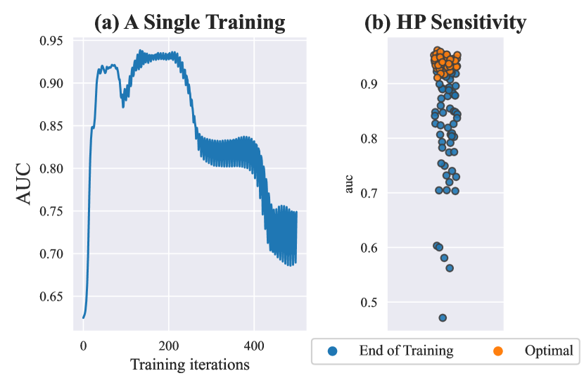
Figure 1: AUC performance of Autoencoder (AE) on dataset vowels. (a) An example of unsupervised training AE. (b) The end-of-training AUC varies across different HP configurations (circles), but the AUC distribution of the optimal iteration during training shows a notable reduction in variation.

In this paper, we revisit the HP sensitivity issue from the perspective of utmost potential of model during training. Our key finding is that the training process can introduce significant variation in model’s detection performance, as depicted in Fig 1 (a). This variation is attributed to the presence of outliers in training data. In this case, even if the model’s performance is stable across the other HPs, training time itself can cause serious HP sensitivity issue (see Fig 1 (b)), as the model with different HP configurations may require varying training iterations to achieve its optimal performance. According to our knowledge, there is no systematic study on training time’s effect on unsupervised OD. Only a few studies [25, 7, 8] employ model ensembles to enhance the robustness of models to training time.

The goal of our research is two-fold. Firstly, our primary objective is to illustrate that training time plays a vital role in reducing HP sensitivity in deep OD models. To this end, we conduct a large-scale analysis of experiments on deep OD models, which quantitatively demonstrates that HP sensitivity in some cases can be greatly alleviated by halting training at the optimal moment. Interestingly, our experimental results also reveal that deep OD models typically require much less training time than previous thought. Secondly, motivated by our finding, we propose a novel internal evaluation metric called loss entropy, which evaluates the model’s performance solely based on the data loss. Through the use of loss entropy, optimal training stop moment can be predicted with remarkable accuracy for the first time. Based on this powerful metric, we devise an automated training stopping algorithm that can dynamically determine the optimal training iteration. Our main contributions are as follows.

• The first systematic study on training time in unsupervised OD: To the best of our knowledge, we are the first to associate HP sensitivity with training time, and investigate how to evaluate a model’s in-training performance without using any validation labels.

• Loss entropy, a novel internal evaluation metric: We propose a novel metric to evaluate the model’s in-training performance solely based on the data loss, which captures the model’s state on learning useful signals from a contaminated training set efficiently. (Sec. 3.2)

• EntropyStop, an automated training stopping algorithm: We develop an automated training stopping algorithm that adapts to the dataset and HP configuration to determine the optimal training iteration. Our algorithm eliminates the need for manual tuning the training iterations and improves the robustness of deep OD algorithms to their HP configuration, while reducing training time by 60-95% compared to naive training. (Sec. 3.3)

• Extensive experiments: We conduct extensive experiments to validate the effectiveness of our approach. The results show that our approach can be applied to diverse deep OD models and datasets to alleviate the HP sensitivity issue and improve the detection performance, while taking much less time than existing solutions. (Sec. 4)

Overall, our contributions provide a comprehensive understanding of the role of training time in deep OD models and offer practical solutions for improving their performance. To foster future research, we open-source all code and experiments at https://github.com/goldenNormal/AutomatedTrainingOD.

2 Related Work

Unsupervised Outlier Detection (OD). Unsupervised OD is a vibrant research area, which aims at detecting outliers in contaminated datasets without any labels providing a supervisory signal during the training [6]. In some literature like [34, 17], “unsupervised outlier/anomaly detection” actually refers to semi-supervised OD by our definition, as their training set only contains normal data. Solutions for unsupervised OD can be broadly categorized into shallow (traditional) and deep (neural network) methods. Compared to traditional counterparts, deep methods are more adept at handling large, high-dimensional and complex data [12]. Despite their relatively recent emergence, multiple surveys have been published to cover the growing literature [5, 30, 32]. However, recent research [8] has shown that popular deep OD methods are highly sensitive to their hyperparameter(s) (HP) while there is no systematical way to tune these HPs, hindering their application in real world.

Model Selection in Unsupervised OD. Various evaluation studies have reported existing outlier detectors to be quite sensitive to their HP choices [8, 1, 4, 11], both traditional and deep detectors. Thus, it promotes some study on selecting a good OD detector with its HP configuration when a new OD task comes, which is called Unsupervised Outlier Model Selection (UOMS) [26]. For example, MetaOD [45] employs meta-learning to select an effective model (i.e. algorithm with its HPs) which has a good performance on similar historical tasks. Some internal (i.e., unsupervised) evaluation strategies have been proposed [10, 27, 28] to evaluate the detection performance of OD detectors, which solely rely on the input data (without labels) and the output (i.e., outlier scores). However, all the above works only focus on the selection of traditional detectors. For a comprehensive study, we investigate the effectiveness of existing UOMS solutions on deep OD in our experiment, compared with our solution.

3 Methodology: Entropy-based Automated Training Stopping

Background. Unsupervised OD presents a collection of $n$ samples $D=\{\textbf{x}_{1},...,\textbf{x}_{n}\}\in\mathbb{R}^{n\times d}$, which consists of inlier set $D_{in}$ (i.e. the normal) and outlier set $D_{out}$. The goal is to train a model $M$ to output outlier score $\textbf{O}:=M(D)\in\mathbb{R}^{n\times 1}$, where a higher $o_{i}$ indicates greater outlierness for $\textbf{x}_{i}$.

Problem (Unsupervised Outlier Training Halting) Given a deep model $M$’s unsupervised training on a contaminated dataset $D\in\mathbb{R}^{n\times d}$ where $T$ is the optimal iteration when $M$ has the best detection performance on $D$ evaluated by ground truth label $\textbf{Y}\in\mathbb{R}^{n\times 1}$. The goal is to halt the training process at iteration $T$ without relying on the label Y and obtain the corresponding prediction $\textbf{O}\in\mathbb{R}^{n\times 1}$.

To clarify, an iteration in this context denotes the process of gradients updates computed on a single batch of training data, while an epoch denotes the process of iterating over all the batches once.

3.1 Basic Assumption

To simplify the problem, we assume the composition of the loss function. This assumption is applicable to a diverse set of deep OD models, as elaborated in a survey [14].

Assumption 3.1 (Loss function).

Training loss can be formulated as $\mathcal{L}(D;\Theta)=\mathcal{J}(D;\Theta)+\mathcal{R}(D;\Theta)$. where $\mathcal{L}$ is the training loss on dataset $D$ and $\Theta$ is the learnable parameters of model $M$; $\mathcal{J}(\cdot)$ and $\mathcal{R}(\cdot)$ denote self-supervised loss and auxiliary loss (e.g. L2-regularization), respectively.

Assumption 3.2 (Alignment).

$\forall\textbf{x}_{i},\textbf{x}_{j}\in D$, if $M(\textbf{x}_{i};\Theta)<M(\textbf{x}_{j};\Theta)$, then $\mathcal{J}(\textbf{x}_{i};\Theta)<\mathcal{J}(\textbf{x}_{j};\Theta)$.

Assumption 3.2 ensures that the rank of learned outlier score function (i.e. $M(\cdot)$) is aligned with self-supervised loss, which is valid for many deep OD models, e.g. AE [2], Deepsvdd [33], NTL [31]. We assume $\mathcal{J}_{\Theta}(\textbf{X};\Theta)\geq 0$ for convenience. If not established, $\mathcal{J}_{\Theta}(\textbf{X};\Theta)^{2}$ can be used as a substitute. As $\mathcal{R}(\cdot)$ serves as the role like regularization, we omit it in the following analysis for simplicity.

3.2 Loss Entropy: An Internal Evaluation Metric

What does the model learn? As model $M$ is trained on a polluted set $D$, learning signals can be classified into useful ones $\{\mathcal{J}(\textbf{x}_{i};\Theta)|\textbf{x}_{i}\in D_{in}\}$ and harmful ones $\{\mathcal{J}(\textbf{x}_{i};\Theta)|\textbf{x}_{i}\in D_{out}\}$.

Overview. We introduce loss entropy to track a model’s progress in learning useful and harmful signals. Firstly, we demonstrate that the model puts more efforts on learning harmful signals only when the outlier’s loss is significantly greater than that of inliers due to "inlier priority" [40]. Drawing on this insight, we analyze the changes in the loss distribution when the model learns different signals. Finally, we propose using the entropy of the loss as the metric to capture such changes.

3.2.1 Inlier Priority: a foundational concept in self-supervised OD

Inlier priority [40, 43] means that the intrinsic class imbalance of inliers/outliers in the dataset will make the deep model prioritize minimizing inliers’ loss when inliers/outliers are indiscriminately fed into the model for training. When $\mathcal{R}(\cdot)$ is ignored, the loss $\mathcal{L}$ of $M$ on $D$ can be written as:

$$\small\mathcal{L}=\mathcal{J}(D;\Theta)=\frac{1}{n}\sum\mathcal{J}(\textbf{x}_{i};\Theta)$$ (1)

Then the corresponding loss on $D_{in}$ and $D_{out}$ can be defined as:

$$\small\mathcal{L}_{{in}}=\mathcal{J}(D_{in};\Theta)=\frac{1}{|D_{in}|}\sum\mathcal{J}(\textbf{x}_{i};\Theta),\quad\textbf{x}_{i}\in D_{in}$$ (2)

$$\small\mathcal{L}_{{out}}=\mathcal{J}(D_{out};\Theta)=\frac{1}{|D_{out}|}\sum\mathcal{J}(\textbf{x}_{i};\Theta),\quad\textbf{x}_{i}\in D_{out}$$ (3)

Inlier priority refers to that $M$ will prioritize minimizing the loss on $D_{in}$, resulting in $\mathcal{L}_{in}<\mathcal{L}_{out}$ constantly during the training process. The priority can be justified in the following two aspects:

Priority due to the larger quantity of inliers. Recalling above Eq 1-3, $M$ aims to minimize the overall loss $\mathcal{L}$, which can be represented as $\mathcal{L}=\frac{|D_{out}|}{n}\mathcal{L}_{out}+\frac{|D_{in}|}{n}\mathcal{L}_{in}$. Since $|D_{in}|\gg|D_{out}|$ usually establishes, the weight of $\mathcal{L}_{in}$ is much larger. Thus, $M$ puts more efforts to minimize $\mathcal{L}_{in}$.

Priority by gradient updating direction. By minimizing the overall loss $\mathcal{L}$, learnable weights $\Theta$ are updated by gradient descent $\overline{g}=\frac{1}{n}\sum g_{i}=\frac{1}{n}\sum\frac{\mathrm{d}\mathcal{J}(\textbf{x}_{i};\Theta)}{\mathrm{d}\Theta}$, where $g_{i}$ is the gradient contributed by $\textbf{x}_{i}$. The effect of gradient update for minimizing $\mathcal{J}(\textbf{x}_{i};\Theta)$ is $g_{i}^{effect}=\frac{<g_{i},\overline{g}>}{|g_{i}|}=|\overline{g}|cos\theta(g_{i},\overline{g})$, where $\theta(g_{i},\overline{g})$ is the angle between two vectors. In most cases, outliers are randomly distributed in the feature space, causing opposing gradient directions, while inliers are densely distributed, leading to more consistent gradient directions. Thus, $\theta(g_{i},\overline{g})$ is smaller for inliers than outliers, resulting in a larger $g_{i}^{effect}$ for $\textbf{x}_{i}\in D_{in}$.This implies that the overall gradient focuses more on reducing $\mathcal{L}_{in}$.

Overall, our analysis confirms that the model prioritizes minimizing $\mathcal{L}_{in}$ when $\mathcal{L}_{in}$ $\approx$ $\mathcal{L}_{out}$ . The model shifts its focus to outliers only when $\mathcal{L}_{out}\gg\mathcal{L}_{in}$.

3.2.2 Loss Entropy: The novel internal evaluation metric

How to evaluate model’s learning state? The model’s detection performance improves with useful signal learning and deteriorates with harmful signal learning. To analyze the model’s learning state at iteration $i$, we quantify the ratio of drop speed between two losses as $\frac{V_{in}^{i}}{V_{out}^{i}}=\frac{\mathrm{d}\mathcal{L}_{in}^{i}}{\mathrm{d}\mathcal{L}_{out}^{i}}$, where $V_{in}^{i}$ and $V_{out}^{i}$ are drop speed of $\mathcal{L}_{in}$ and $\mathcal{L}_{out}$ at iteration $i$, respectively. Since learning signals is essentially the loss reduction, $\frac{V_{in}^{t_{i}}}{V_{out}^{t_{i}}}$ tells which signals $M$ learns more at iteration $i$. However, $\mathcal{L}_{in}^{{i}}$ and $\mathcal{L}_{out}^{{i}}$ cannot be calculated without the ground truth labels.

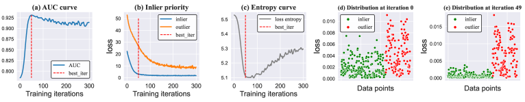
Figure 2: An example of AE model’s training on the dataset Ionosphere with 300 iterations. The optimal iteration evaluated by AUC is the $49^{th}$ iteration. The y-axis of two scatter plots (i.e. (d) and (e)) is normalized data loss value $p_{i}^{loss}\in\mathcal{P}^{loss}$.

Changes in the loss distribution. Though direct calculation is infeasible, the loss distribution over the dataset at iteration $i$ can reflect $\frac{V_{in}^{i}}{V_{out}^{i}}$ due to the intrinsic class imbalance. When $V_{in}^{i}\gg V_{out}^{i}$, then the majority of loss (i.e. $\{\mathcal{J}(\textbf{x}_{i};\Theta)|\textbf{x}_{i}\in D_{in}\}$) has a dramatic decline while the minority of loss (i.e. $\{\mathcal{J}(\textbf{x}_{i};\Theta)|\textbf{x}_{i}\in D_{out}\}$) remains relatively large, leading to a steeper distribution (See the example in Figure 2). Conversely, when $V_{in}^{i}\ll V_{out}^{i}$, the distribution will change towards flatter. Thus, the changes in the shape of the distribution can give some valuable insights into the training process.

Our metric. We employ the entropy of loss distribution $\mathcal{P}^{loss}$ to capture such changes, where entropy [37] is a natural metric to measure the flatness of an arbitrary probability distribution $\mathcal{P}$:

$$\small entropy(\mathcal{P})=\sum_{p_{i}\sim\mathcal{P}}(p_{i}\log{p_{i}}),\quad s.t.\sum_{p_{i}\sim\mathcal{P}}p_{i}=1,p_{i}\geq 0$$ (4)

Basically, the more flat or uniform $\mathcal{P}$ is, the larger $entropy(\mathcal{P})$ is. To convert $\{\mathcal{J}(\textbf{x}_{i};\Theta)|\textbf{x}_{i}\in D\}$ into $\mathcal{P}^{loss}$, we adopt $\sum_{\textbf{x}_{i}\in D}\mathcal{J}(\textbf{x}_{i};\Theta)$ to normalize each loss value as $p_{i}^{loss}=\frac{\mathcal{J}(\textbf{x}_{i};\Theta)}{\sum_{\textbf{x}_{i}\in D}\mathcal{J}(\textbf{x}_{i};\Theta)}$.

To achieve efficient and consistent entropy measurement, we randomly sample $N_{eval}$ instances from $D$ to create an evaluation set $D_{eval}$ before training and calculate $entropy(\mathcal{P}^{loss})$ on $D_{eval}$ per iteration. To ensure accuracy, techniques that introduce randomness (e.g. dropout) are disabled when computing $entropy(\mathcal{P}^{loss})$, although they can still be used during training. Finally, loss entropy is expected to have a negative correlation with variation in detection performance. Several examples in Figure 3 show that loss entropy provides a reliable measure of variations in AUC.

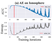
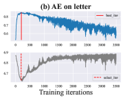
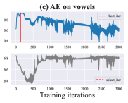
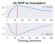
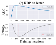
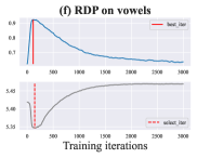
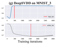
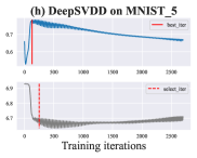
Figure 3: Examples of AUC and loss entropy curves during the training. The “select_iter” denotes the iteration selected by EntropyStop.

3.3 EntropyStop: Automated Training Stopping Algorithm

In this subsection, we will illustrate the primary idea for selecting the optimal iteration from the entropy curve (see Fig 3), and propose a training stopping algorithm to automate this process.

Loss entropy primarily reflects the direction of variation in detection performance, rather than the precise amount of variation. In most cases, the model prioritizes learning useful signals from inliers, leading to a gradual decrease in loss entropy. However, when the model shifts its focus on outliers, the entropy starts to rise, suggesting that training should be terminated. Although the model has a small potential to re-focus on inliers to improve detection performance, our metric cannot measure the extent of this improvement. Therefore, we opt to stop training as soon as the entropy stops decreasing. We present our problem formulation for selecting the optimal iteration below.

Problem Formulation. Suppose $\mathcal{E}=\{e_{j}\}_{j=0}^{E}$ denotes the entropy curve of model $M$. When $M$ finishs its $i^{th}$ training iteration, only the subcurve $\{e_{j}\}_{j=0}^{i}$ is available. The goal is to select a point $e_{i}\in\mathcal{E}$ as early as possible that (1) $\forall j<i,e_{i}<e_{j}$; (2) the subcurve $\{e_{j}\}_{j=0}^{i}$ has a downtrend; (3) $\forall q\in(i,k+i)$, the subcurve $\{e_{j}\}_{j=i}^{q}$ has no downtrend.

Algorithm. In above formulation, $k$ is the patience parameter of algorithm. As an overview, our algorithm continuously explores new points within $k$ iterations of the current lowest entropy point $e_{i}$, and tests whether the subcurve between the new point and $e_{i}$ exhibits a downtrend. Specifically, when encountering a new point $e_{q}$, we calculate $G=\sum_{j=i+1}^{q}(|e_{j}-e_{j-1}|)$ as the total variations of the subcurve $\{e_{j}\}_{j=i}^{q}$ and the downtrend of the subcurve is then quantified by $\frac{e_{i}-e_{q}}{G}$. Particularly, if the subcurve is monotonically decreasing, then $\frac{e_{i}-e_{q}}{G}=1$. To test for a significant downtrend, we use a threshold parameter $R_{down}\in(0,1)$. Only when $\frac{e_{i}-e_{q}}{G}$ exceeds $R_{down}$ will $e_{q}$ be considered as the new lowest entropy point. The complete process is shown in Algorithm 1.

Input: Model $M$ with learnable parameters $\Theta$, patience parameter $k$, downtrend threshold $R_{down}$, dataset $D$, iterations T, evaluation set size $N_{eval}$

Output: Outlier score list O

1 Initialize the parameter $\Theta$ of Model $M$;

2 Random sample $N_{eval}$ instances from $D$ as the evaulation set $D_{eval}$ ;

3 $G\leftarrow 0;$ $patience\leftarrow 0;$ $\Theta_{best}\leftarrow\Theta;$ ;

4

5$e_{0}\leftarrow entropy^{loss}(\{\mathcal{J}(\textbf{x}_{i};\Theta),\textbf{x}_{i}\in D_{eval}\});$ $e^{min}\leftarrow e_{0}$;

;

  /* Model Training */

6 for $j:=1\rightarrow T$ do

7       Random sample a batch of training data $D_{batch}$ ;

8       Calculate $\mathcal{L}_{train}=\mathcal{J}(D_{batch};\Theta)+\mathcal{R}(D_{batch};\Theta)$ ;

9       Optimize the parameters $\Theta$ by minimizing $\mathcal{L}_{train}$;

10       $e_{j}\leftarrow entropy^{loss}(\{\mathcal{J}(\textbf{x}_{i};\Theta),\textbf{x}_{i}\in D_{eval}\})$;

11       $G\leftarrow G+|e_{j}-e_{j-1}|$;

12       if  $e_{j}<e^{min}$ and $\frac{e^{min}-e_{j}}{G}>R_{down}$  then

13             $e^{min}\leftarrow e_{j};$ $G\leftarrow 0;$ $patience\leftarrow 0;$ $\Theta_{best}\leftarrow\Theta;$

14      else

15             $patience\leftarrow patience+1$;

16            

17       end if

18      if $patience=k$ then

19            break

20       end if

21      

22 end for

Return: $M(D;\Theta_{best})$

Algorithm 1 EntropyStop: An automated training stopping algorithm

Two new parameters are introduced, namely $k$ and $R_{down}$. $k$ represents the patience for searching the optimal iteration, with larger value improving accuracy at the expense of longer training time. Then, $R_{down}$ sets the requirement for the significance of downtrend. Apart from these two parameters, learning rate is also critical as it can significantly impact the training time. We recommend setting $R_{down}$ within the range of $[0.01,0.1]$, while the optimal value of $k$ and learning rate is associated with the actual entropy curve. We provide a guidance on tuning these HPs in Appx A.1.

Time Complexity. The time complexity for each iteration is $O(\mathcal{J}(D_{eval};\Theta))+O(|D_{eval}|)$, including the computation of $\{\mathcal{J}(\textbf{x}_{i};\Theta),\textbf{x}_{i}\in D_{eval}\}$ and $entropy(\mathcal{P}^{loss}_{eval})$.

3.4 Inapplicability

Our metric and algorithm are based on inlier priority, but it is crucial to acknowledge that outliers may exihibit similar patterns to inliers. For instance, local outliers may exist in the peripheral region of the normal class, resulting in gradient directions that are comparable to those of normal data points. To study this, we conducted a investigation of various outlier types in Sec 4.3, which indicates that our approach has limited effectiveness for local outliers. Nevertheless, for other types of outliers, such as cluster and global outliers, our approach can significantly boost performance by halting training at the optimal iteration.

Our method cannot be combined with pre-training techniques. As the learnable parameters $\Theta$ are significantly influenced by pre-training, the entropy curves during training may be inaccurate.

4 Experiments

Evaluation Metrics. We evaluate the detection performance by AUC [15].We adopt $Score_{AUC}$ [35] to indicate the aggregated scores across all datasets:

$$\small Score_{AUC}(A^{(i)})=\frac{1}{j}\sum_{j}\frac{AUC(A^{(i)},D^{(j)})}{max_{p}AUC(A^{(p)},D^{(j)})}$$

where $A^{(i)}$,$D^{(j)}$ represent the $i^{th}$ algorithm and the $j^{th}$ dataset, respectively.

Computing Infrastructures. All experiments are conducted on a computer with Ubuntu 18.04 OS, AMD Ryzen 9 5900X CPU, 62GB memory, and an RTX A5000 (24GB GPU memory) GPU.

4.1 TestBed

Table 1: Dataset statistics

Name	Type	# Pts	Dim	% Outl
Ionosphere	tabular	351	32	35.9
letter	tabular	1600	32	6.25
vowels	tabular	1456	12	3.43
MNIST-3	image	7357	$28\times 28$	16.6
MNIST-5	image	6505	$28\times 28$	16.6

Datasets. Experiments are based on 3 tabular datasets from ADbenchmark [12] as well as 2 image datasets from MNIST (see Table 1). For image datasets, we pick one class as the inliers and downsample the other classes to constitute the outliers. Details on dataset description and preparation can be found in Appx. A.2.1.

Models. We analyze the sensitivity of HPs for AE [2], RDP [39], DeepSVDD [33]. We list the studied HPs in Table 2, and provide detailed descriptions in Appx. A.2.2. We define a grid of 2-3 values for each HP and train each deep OD method with all possible combinations. To evaluate the utmost potential of model during its training, we evaluate its AUC on the whole dataset after each training iteration while the loss entropy is computed on a pre-sampled evaluation set at the same time.

Table 2: Deep OD for studying HP sensitivity. (See Appx. A.2.2 for list of grid values per HP.)

Method	Type	List of HPs	# models
AE [2]	tabluar & image	act_func $\cdot$ dropout, h_dim $\cdot$ lr $\cdot$ layers $\cdot$ epoch	64
RDP [39]	tabluar	out_c $\cdot$ lr $\cdot$ dropout $\cdot$ filter $\cdot$ epoch	72
DeepSVDD [33]	image	conv_dim $\cdot$ fc_dim $\cdot$ relu_slope $\cdot$ epoch,lr $\cdot$ wght_dc	64

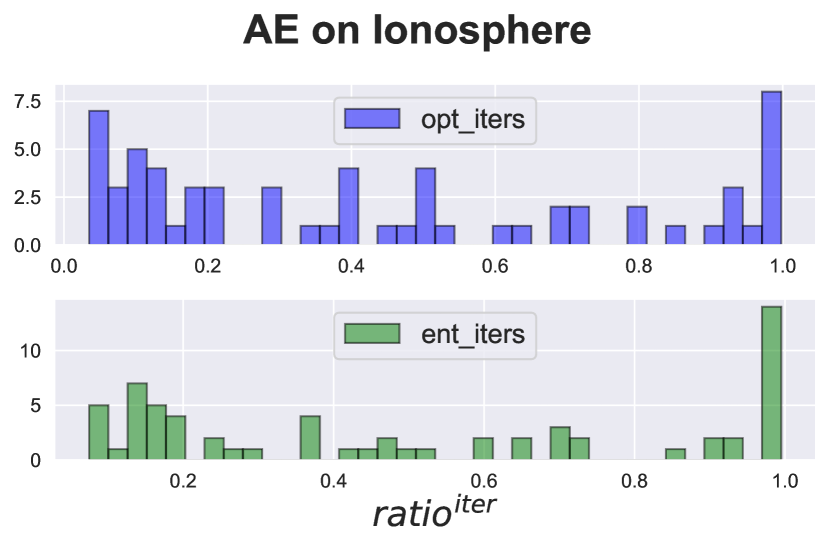
Figure 4: Iterations selected by $Optimal$ and $Entropy$ accross 64 HP configs. The value is normalized by iterations of Naive training.

Baselines. We report the end-of-training AUC and the optimal AUC during training as Naive and Optimal, respectively. We denote the AUC obtained by our EntropyStop as Entropy. For UOMS solutions, Xie-Beni index (XB) [29], ModelCentrality (MC) [21], and HITS [26] are the baselines for comparison. For ensemble solutions, we select the deep hyper-ensemble AE model ROBOD [8] and the SOTA traditional detector IsolationForest (IF) [23]. Note that Naive, Optimal, and Entropy have AUC scores for each HP configuration, whereas the UOMS solutions only produce a single AUC score for a given dataset and algorithm pair. For EntropyStop, we set $R_{down}$ to 0.1 while $k$ varies according to model and dataset. Since ROBOD is essentially an AE ensemble, we use different layers, hidden units as well as random seeds to create an ensemble of AE models while analyzing its performance on the remaining HPs of AE. We keep IF at a default setting. More details are available in Appx. A.2.2.

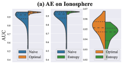
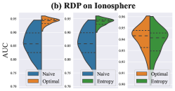
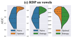
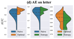
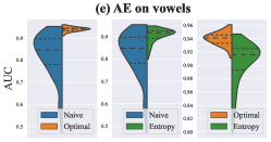
Figure 5: Comparison of AUC distribution of Naive, Optimal, and Entropy across varing HP configurations. Our Entropy achieves a similar effect as Optimal without the ground-truth labels in (a), (b),(c),(d) and (f) (totally 344 different trainings). Remaining figures in Fig A6 Appx. A.3.2.

4.2 Results

The experiments are conducted three times and the average results are reported in Table 4. Q1: Does training time significantly impact the model’s performance? For training AE/RDP on tabular datasets (see Fig 5), by solely attaining the optimal performance during training, the HP sensitivity issue is greatly mitigated, revealing that training time is the primary factor to cause HP sensitivity. For training DeepSVDD on MNIST (see Fig A6 in Appx. A.3.2), due to the existence of other sensitive HPs, Optimal only has a slight reduction in AUC variation, but it greatly improves the overall AUC. These results demonstrate the significant impact of training time on model’s performance. In Fig 4, the optimal AUC iteration has a diverse distribution, indicating that the model with different HPs requires varying training iterations to achieve its optimal performance.

Table 3: Expected training time on each dataset, normalized by training time of Naive AE. (Smaller is better)

Dataset	EntropyAE	ROBOD	UOMS(AE)	IF
Ionosphere	0.39	4.16	64.00	0.13
letter	0.27	4.15	64.00	0.04
vowels	0.15	4.08	64.00	0.04
MNIST-3	0.04	4.79	64.00	0.01
MNIST-5	0.05	4.80	64.00	0.01

Q2: Does our approach can achieve a similar effect to Optimal? For RDP, Entropy achieves a surprisingly similar effect to Optimal on 3 datasets with 72 diverse HP configs (totally 216 trainings) in the absence of labels, highlighting its effectiveness. For AE, the similar outstanding effect is observed on Ionosphere and letter (totally 128 trainings). Though there is a gap between Optimal and Entropy on vowels for AE, Entropy still significantly reduces the HP sensitivity of Naive and improve the overall AUC. We acknowledge its limitation in capturing the optimal performance of AE on MNIST. However, more than 95% of training time is saved on MNIST due to the early detection of training convergence, as shown in Table 3. For DeepSVDD, Entropy also achieves a similar effect to Optimal. Overall, Entropy improves the AUC of Naive on all models and datasets, as shown in Table 4, while save 61-96% training time according to Table 3. The similar time-saving results are also observed in RDP and DeepSVDD. In fact, it averagely saves more time on a larger dataset as the same training epochs will result in more training iterations under a fixed batch size. In Fig 4, it shows that Entropy adopts to different HP configurations to select the optimal iterations.

Table 4: AUC performance of baselines for Unsupervised OD. Highlighted in red bold and blue italics are the best and runner-up. Standard deviation of Naive, Entropy and ROBOD denotes performance variance across HP configs while that of UOMS (i.e. XB, MC and HITS) and IF denotes the performance variance across different random seeds.

Dataset	Model	Naive	Entropy (Ours)	XB [26]	MC [26]	HITS [26]	ROBOD [8]	IF [23]
Ionosphere	AE	0.878$\pm$0.123	0.944$\pm$0.009	0.884$\pm$0.056	0.946$\pm$0.004	0.939$\pm$0.006	0.919$\pm$0.028	0.853$\pm$0.008
	RDP [39]	0.859$\pm$0.053	0.938$\pm$0.013	0.871$\pm$0.054	0.810$\pm$0.039	0.856$\pm$0.004
letter	AE	0.799$\pm$0.091	0.838$\pm$0.032	0.770$\pm$0.005	0.868$\pm$0.007	0.870$\pm$0.005	0.815$\pm$0.037	0.616$\pm$0.039
	RDP	0.689$\pm$0.103	0.801$\pm$0.032	0.601$\pm$0.106	0.597$\pm$0.048	0.72$\pm$0.027
vowels	AE	0.824$\pm$0.101	0.902$\pm$0.033	0.701$\pm$0.184	0.912$\pm$0.006	0.899$\pm$0.015	0.872$\pm$0.034	0.749$\pm$0.008
	RDP	0.779$\pm$0.099	0.901$\pm$0.034	0.669$\pm$0.054	0.731$\pm$0.048	0.791$\pm$0.028
MNIST-3	AE	0.826$\pm$0.009	0.835$\pm$0.009	0.819$\pm$0.001	0.825$\pm$0.002	0.822$\pm$0.002	0.830$\pm$0.004	0.755$\pm$0.021
	DeepSVDD [33]	0.748$\pm$0.047	0.805$\pm$0.025	0.665$\pm$0.022	0.801$\pm$0.014	0.818$\pm$0.012
MNIST-5	AE	0.758$\pm$0.006	0.762$\pm$0.009	0.762$\pm$0.011	0.759$\pm$0.002	0.755$\pm$0.001	0.763$\pm$0.009	0.660$\pm$0.008
	DeepSVDD	0.684$\pm$0.053	0.748$\pm$0.042	0.668$\pm$0.007	0.725$\pm$0.039	0.747$\pm$0.019
Score		0.920	0.994	0.870	0.935	0.964	0.971	0.840

Q3: How does our approach compare to UOMS solutions? Though our approach does not consistently outperform UOMS solutions, it is important to note that the comparison is somewhat unfair. The entry of Entropy in Table 4 represents an expected AUC for a model in a random HP configuration, while UOMS (i.e., XB, MC, HITS) selects the “best“ one from a pool of all models, resulting in that their training time is several magnitudes longer than ours (see Table 3). Additionally, Entropy exhibits superior performance when dealing with RDP that employs random-distance as its outlier score function. Our goal is to emphasize the significance of training time in HP sensitivity and offer a lightweight solution to mitigate the HP sensitivity issue. By solely determining the optimal iteration, our approach surpasses UOMS in terms of overall effectiveness.

Q4: how does our approach compare to ensemble solutions? Since ROBOD is essentially an AE ensemble, we compare it to EntropyAE (i.e. AE with EntropyStop). As shown in Table 4, EntropyAE exceeds ROBOD on 4 datasets (i.e. three tabular datasets and MNIST-3) and takes only 1-10% training time of ROBOD (see Table 3). For MNIST-5, they have the same performance (only 0.001 difference in AUC). This result verifies the effectiveness of our approach in unleashing the potential of AE. In terms of IF, its performance falls far behind the other baselines on these datasets.

4.3 Further Investigation

Table 5: Effectiveness of EntropyStop on heterogeneous outliers at varing outlier ratio. $P_{auc}\leq 0.05$ means the existence of significant improvement. (See detailed results in Appx. A.3.1)

Type	Outl	Naive	Entropy	$P_{auc}$	time
cluster	0.1	0.646	0.864	0.000	0.203
cluster	0.4	0.559	0.836	0.000	0.168
global	0.1	0.944	0.981	0.000	0.479
global	0.4	0.917	0.967	0.000	0.335
local	0.1	0.891	0.901	0.522	0.351
local	0.4	0.910	0.900	0.998	0.390

Applicability and Limitations. To gain a more comprehensive understanding of our approach, we conduct investigations on its effectiveness on heterogeneous outliers at varying outlier ratios. We inject local, global, and cluster outliers separately into 19 datasets (see Appx. A.2.3) from [12], using the default settings of injection algorithms in [12], with outlier ratios set to 0.1 and 0.4. The main results are presented in Table 5, along with the p-values obtained from one-sided paired Wilcoxon signed rank tests. Our findings demonstrate that our approach is highly effective on cluster outliers, significantly improving performance on almost all 19 datasets (see Table A5-A6 in Appx. A.3.1). For global outliers, our approach also significantly improves performance, albeit to a lesser extent. However, we observed limited effectiveness in detecting local outliers, as they exhibit similar patterns and gradients to those of inliers, leading to the failure of inlier priority. On the other hand, our method continues to enhance model detection even at an outlier ratio of 0.4, highlighting its robustness to varying outlier ratios. Thus, the type of outlier is more critical for our approach. We recommend that newly developed deep OD methods integrate our approach while verifying the type of outliers and the discrepancy of outlier gradients from inlier gradients.

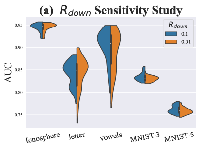
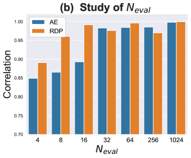
Figure 6: (a) The AUC distributions of EntropyAE with two different $R_{down}$ on 5 datasets. (b) The pearson correlation between entropy curve computed on the whole dataset and the evaluation set with size $N_{eval}$. Fig A5 in Appx. A.3.2 offers a more intuitive display.

Parameter Sensitive Study. We study the sensitivity of our approach to $R_{down}$ and $N_{eval}$. Firstly, we set $R_{down}$ to 0.1 and 0.01, exploring the corresponding performance of EntropAE (i.e. AE with EntropyStop) on 5 datasets in Fig 6 (a). It shows that the two AUC distributions of EntropAE are similar on all datasets, indicating that $R_{down}$ does not significantly influence the effectiveness. Next, we investigate how large the evaluation set needs to be to ensure accurate loss entropy calculation. To measure accuracy, we compute the pearson correlation of the entropy curve computed on the entire dataset and the evaluation set with size $N_{eval}$. We train AE and RDP on vowels dataset. As depicted in Fig 6 (b), when $N_{eval}\geq 32$, the correlation can exceed 0.96, indicating that loss entropy can be accurately computed without the requirement of a large $N_{eval}$.

5 Conclusion

In this paper, we systematically study the significance of training time in unsupervised OD and propose a novel, efficient metric as well as a training stopping algorithm that can automatically identify the optimal training iterations without requiring any labels. Our research demonstrates that hyperparameter (HP) sensitivity in deep OD can be attributed to training time in certain cases. By halting the training at the optimal moment, the HP sensitivity issue can be greatly mitigated. We hope our insights would benefit the future research in unsupervised OD.

The limitation of our work is the absence of exhaustive theoretical justification for inlier priority and inadequate analysis for the effectiveness of detecting different types of outliers. However, the main focus of our paper is to emphasize the importance of training time in HP sensitivity. In the future, we are committed to conducting an in-depth investigation of cases where inlier priority does not hold and providing a more comprehensive analysis of detecting heterogeneous outliers.

Appendix A Appendix

A.1 Guidelines for tuning parameters of EntropyStop

In this section, we provide guidelines on how to tune the hyperparameters (HPs) of EntropyStop when working with unlabeled data. The three key parameters are the learning rate, $k$, and $R_{down}$. The learning rate is a crucial factor as it significantly impacts the training time. $k$ represents the patience for finding the optimal iteration, with a larger value improving accuracy but also resulting in a longer training time. $R_{down}$ sets the requirement for the significance of the downtrend.

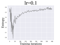
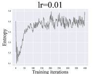
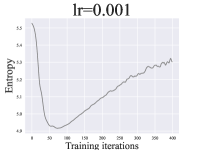
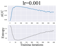
Figure A1: The loss entropy curve of training Autoencoder (AE) on dataset Ionosphere with different learning rate.

Tuning learning rate. When tuning these parameters, the learning rate should be the first consideration, as its value will determine the shape of the entropy curve, as shown in Figure A1. For illustration purposes, we first set a large learning rate, such as 0.1, which is too large for training autoencoder (AE). This will result in a sharply fluctuating entropy curve, indicating that the learning rate is too large. By reducing the learning rate to 0.01, a less fluctuating curve during the first 50 iterations is obtained, upon which an obvious trend of first falling and then rising can be observed. Based on the observed entropy curve, we can infer that the training process reaches convergence after approximately 50 iterations. Meanwhile, the optimal iteration for achieving the best performance may occur within the first 25 iterations. However, the overall curve remains somewhat jagged, indicating that the learning rate may need to be further reduced. After reducing the learning rate to 0.001, we observe a significantly smoother curve compared to the previous two, suggesting that the learning rate is now at an appropriate level.

A good practice for tuning learning rate is to begin with a large learning rate to get a overall view of the whole training process while the optimal iteration can be located. For the example in Fig A1, it is large enough to set learning rate to 0.01 for AE model. Then, zoom out the learning rate to obtain a smoother curve and employ EntropyStop to automatically select the optimal iteration.

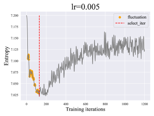
Figure A2: The example of fluctuations (or rises) during the downtrend of entropy curve when training AE on dataset vowels. The value of $k$ should be set larger than the width of all fluctuations.

Tuning $k$ and $R_{down}$. After setting the learning rate, the next step is to tune $k$. If the entropy curve is monotonically decreasing throughout the downtrend, then $k=1$ and $R_{down}=1$ will suffice. However, this is impossible for most cases. Thus, an important role of $k$ and $R_{down}$ is to tolerate the existence of small rise or fluctuation during the downtrend of curve. Essentially, the value of $k$ is determined by the maximum width of the fluctuations or small rises before encounting the opitmal iteration. As shown in Fig A2, the orange color marks the fluctuation area of the curve before our target iteration. The value of $k$ should be set larger than the width of all these fluctuations. For the example in Fig A2, as long as $k\geq 50$ , EntropyStop can select the target iteration.

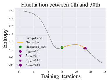
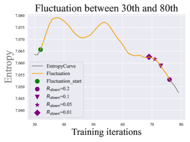
Figure A3: Explanation of the effect of $R_{down}$ in tolerating the existence of fluctuations in the entropy curve shown in Figure A2.

Regarding $R_{down}$, setting it to 0.1 is sufficient in most cases. In Sec. 4.3 of our primary paper, our sensitivity study results verify that the EntropyStop algorithm is not sensitive to $R_{down}$ when its value lies in the range of $[0.01,0.1]$. A visualization of the effect of $R_{down}$ is depicted in Figure A3. When a small fluctuation (or rise) occurs during the downtrend of the curve, suppose $e_{i}$ is the start of this fluctuation. Then, the new lowest entropy points $e_{q}$ that satisfies the downtrend test of varying $R_{down}$ is close to each other. This explains the robustness of EntropyStop to $R_{down}$.

Owning to the effectiveness of $k$ and $R_{down}$ in tolerating the fluctuations, even the entropy curve is not smooth enough due to a large learning rate, the target iteration can still be selected by EntropyStop.(see Fig A4). Nevertheless, we still recommend fine-tuning the learning rate to achieve a smooth entropy curve, which will ensure a stable and reliable training process.

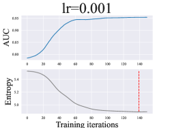
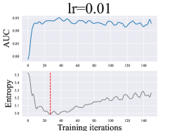
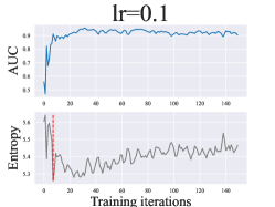
Figure A4: The effect of tolerating the fluctuations when $k$ is set to 50 and $R_{down}$ is set to 0.1 for the training of AE on the dataset Ionosphere. The displayed training process only includes the first 150 iterations. The red dashed line marks the iteration selected by EntropyStop.

In Sec. 4.1 of our primary paper, it is sufficient for AE on all 5 datasets when $k$=100. In finer granularity, $k$ can be set to 25 for the dataset Ionosphere and MNIST to further save training time.

A.2 Details on Experiment Setup

A.2.1 Dataset Description for Primary Experiment

We conduct our experiment in Sec. 4.1 based on 3 tabular datasets from [12] (available at https://github.com/Minqi824/ADBench) and 2 image datasets from MNIST. For tabular datasets, we employ StandardScaler in sklearn.preprocessing to standardize the feature of each dataset. For image dataset, we employ the open-source code from [8] (available at https://github.com/xyvivian/robod) to preprocess the image dataset and generate the outliers. In specific, the global contrast normalization is employed to individual images. The inliers are assigned the label 0 and all classes other than the inlier class will be marked with 1, indicating the outlier class. We choose Digit ‘3’ and ‘5’ as the inlier-class, respectively, while the remaining classes are down-sampled to constitute the outliers.

A.2.2 Hyperparameter Configurations

Regarding the implementation of deep OD method, we utilize open-source code available for RDP and DeepSVDD, two well-established algorithms in outlier detection research. Specifically, for RDP, we use the original open-source code. In the case of DeepSVDD, we employ the open-source code provided by the authors of the ROBOD paper [8]. We develop our own implementation for AE.

For RDP, we employ a training configuration where 30 mini-batch iterations are considered to be a single training epoch. The reason is the existence of parameter “filter” in RDP , which will filter out possible outliers per epoch. Therefore, we keep the consistency training configuration with the original implementation provided in the RDP open-source code.

Model HP Descriptions and Grid of Values.

Table A1: We define a grid of 2-3 unique values for each hyperparameter (HP) of each deep OD method studied.The author-recommended value or the default values in their code is marked in bold and underlined.

Method (#models)	Hyperparameter	Grid	#values
AE (64)	act_func	[relu, sigmoid]	2
	dropout	[0.0, 0.2]	2
	h_dim	[64, 256]	2
	lr	[0.005, 0.001]	2
	layers	[2, 4]	2
	epoch	[100, 500]	2
RDP (72)	out_c	[25,50,100]	3
	lr	[0.1, 0.01]	2
	dropout	[0.0, 0.1]	2
	filter	[0.0, 0.05, 0.1]	3
	epoch	[100, 500]	2
DeepSVDD (64)	conv_dim	[ 8,16]	2
	fc_dim	[16, 64	2
	relu_slope	[0.1, 0.001]	2
	epoch	[100, 250]	2
	lr	[1e-4, 1e-3]	2
	wght_dc	[1e-5, 1e-6]	2

• AE:

  1. act_func: the activation function employed after the first layer of encoder

  2. dropout: the possibility of dropping out the nodes in hidden layer during the training

  3. h_dim: the dimension of hidden layers

  4. lr: the learning rate during the training

  5. layers: the number of hidden layers

  6. epoch: number of training epochs

• RDP:

  1. out_c: the dimension of random projection space

  2. lr: the learning rate during the training

  3. dropout: the possibility of dropping out the nodes in hidden layer during the training

  4. filter: the percent of outliers to be filtered out per epoch

  5. epoch: number of training epochs

• DeepSVDD:

  1. conv_dim: the number of output channels generated by the first convolutional encoder layer. Following this layer, the number of channels will expand at a rate of 2.

  2. fc_dim: the output dimension of the fully connected layer between convolutional encoder layers and decoder layers, in the LeNet structure [19].

  3. relu_slope: DeepSVDD utilizes leaky-relu activation to avoid the trivial, uninformative solutions [33]. Here we alter the leakiness of the relu sloping.

  4. epoch: number of training epochs

  5. lr: the learning rate during the training

  6. wght_dc: weight decay rate

HP Configuration of Baselines.

For EntropyStop, we set $N_{eval}=1024$ and $R_{down}=0.1$ for all deep OD methods and datasets. The values of $k$ are listed in Table A2.

Table A2: The setting of $k$ for EntropyStop. There are 2 different learning rates for each deep OD method and the value of $k$ is set according to different learning rate as well.

Method	Dataset	$k$ for small lr	$k$ for large lr
AE	Ionosphere	25	25
	letter	100	100
	vowels	100	100
	MNIST-3	25	25
	MNIST-5	25	25
RDP	Ionosphere	50	50
	letter	750	150
	vowels	750	150
DeepSVDD	MNIST-3	100	100
	MNIST-5	100	100

For the implementation of Unsupervised Outlier Model Selection (UOMS) [26] solutions (i.e. baseline XB, MC and HITS), we use the open-source code from [26]. For XB, we give it the advantage to know the outlier ratio of dataset. For MC, the Kendall $\tau$ coefficient is employed to calculate the similarity of outlier score list.

For AE ensemble model ROBOD, we use the open-source code from its original paper [8]. We employ their original code implementation of ensembling varying widths and depths of AE, alongside different random seeds, resulting in a total of 16 models for ensemble. The remaining HPs of AE are used to analyze its expected performance.

For Isolation Forest (IF), we use its implementation from PYOD [44] and adopt its default HP setting, which ensembles 100 different trees.

A.2.3 Experiment setting for Further Investigation

For our experiment in Sec. 4.3 of primary paper, we use 19 datasets as well as outlier injection approach from ADbench [12] to study the effectiveness in detecting heterogeneous outliers under varying outlier ratio. The original dataset statistics of 19 datasets are shown in Table A.2.3. We remove the original outliers in the dataset and separately inject cluster, global and local outliers into the dataset, while controlling the outlier ratio to 0.1 and 0.4. We adopt the default value of parameters for the injection approach (see below definition). In Sec. 4.3 Table 5, we report the results of EntropyAE (i.e. AE with our EntropyStop) with a specific HP configuration (listed in Table A.2.3) on detecting different types of outliers. The detailed detection results of Table 5 are available in Appx. A.3.1.

Table A3: 19 datasets for heterogeneous outliers injection.

Dataset	Num Pts	Dim	% Outlier
breastw	683	9	34.99
cardio	1831	21	9.61
Cardiotocography	2114	21	22.04
fault	1941	27	34.67
glass	214	7	4.21
Hepatitis	80	19	16.25
InternetAds	1966	1555	18.72
Ionosphere	351	32	35.90
letter	1600	32	6.25
Lymphography	148	18	4.05
Pima	768	8	34.90
Stamps	340	9	9.12
vertebral	240	6	12.50
vowels	1456	12	3.43
WBC	223	9	4.48
WDBC	367	30	2.72
wine	129	13	7.75
WPBC	198	33	23.74
yeast	1484	8	34.16

Table A4: The hyperparameter of EntropyAE for the experiment in Sec. 4.3 and Table 5.

Hyperparameter	value
act_func	relu
dropout	0.2
h_dim	64
num_layer	2
lr	0.001
epoch	250
batch size	256
$N_{eval}$	1024
$k$	100
$R_{down}$	0.1

Definition and Generation Process of Three Types of Outliers Used in ADBench [12] :

• Local Outlier refer to the outliers that are deviant from their local neighborhoods [3]. The injection method follows the GMM procedure [36] to generate synthetic normal samples, and then scale the covariance matrix $\hat{\Sigma}=\alpha\hat{\Sigma}$ by a scaling parameter $\alpha=5$ to generate local outlier.

• Global Outlier are more different from the normal data [16], generated from a uniform distribution $Unif(\alpha\cdot min(\textbf{X}^{k}),\alpha\cdot max(\textbf{X}^{k}))$, where the boundaries are defined as the $min$ and $max$ of an input feature, e.g., $k$-th feature $\textbf{X}^{k}$, and $\alpha=1.1$ controls the outlyingness.

• Cluster Outlier, also known as group outliers [20], exhibit similar characteristics [22]. The injection method scales the mean feature vector of normal samples by $\alpha=5$, i.e., $\hat{\mu}=\alpha\hat{\mu}$, where $\alpha$ controls the distance between outlier clusters and the normal, and use the scaled GMM to generate outliers.

A.3 Detailed Experiment Results

A.3.1 Detailed Results for heterogeneous outliers at varying outlier ratios

In this section, we provide the detailed results of Table 5 in Sec. 4.3, which are shown in Table A5 - A10.

Results. Our results demonstrate the effectiveness of our proposed approach in mitigating the impact of cluster outliers on AE performance. Specifically, our approach successfully prevents AE from learning harmful signals from cluster outliers on all 19 datasets, which would otherwise lead to a significant decline in performance when using the Naive training method. For global outliers, our approach improves the overall performance with a less significant level. This is due to the fact that the in-training performance of AE on detecting global outliers is not sensitive to the presence of harmful signals, resulting in only a slight improvement in performance with our approach. However, it should be noted that our approach is not applicable to detecting local outliers, as they behave similarly to inliers when the reconstruction loss of AE is computed.

Table A5: AUC Performance of EntropyAE and NaiveAE on detecting cluster outliers at 0.1 outlier ratio. Column nai_time and en_time denotes the training time of Naive and Entropy in seconds.

Dataset	Entropy	Naive	en_time	nai_time
Cardiotocography	0.799	0.760	0.286	2.278
Hepatitis	1.000	0.397	0.152	0.295
InternetAds	0.047	0.159	0.376	2.249
Ionosphere	0.953	0.685	0.154	0.290
Lymphography	0.997	0.531	0.152	0.289
Pima	0.997	0.873	0.183	0.887
Stamps	0.941	0.764	0.155	0.569
WBC	0.926	0.705	0.155	0.286
WDBC	0.923	0.579	0.167	0.576
WPBC	0.484	0.251	0.153	0.287
breastw	1.000	0.713	0.181	0.567
cardio	0.692	0.744	0.372	2.275
fault	1.000	0.754	0.161	1.770
glass	0.959	0.889	0.161	0.308
letter	1.000	0.778	0.180	2.017
vertebral	0.944	0.660	0.161	0.287
vowels	1.000	0.798	0.157	1.987
wine	1.000	0.438	0.161	0.291
yeast	0.763	0.803	0.378	1.414

Table A6: AUC Performance of EntropyAE and NaiveAE on detecting cluster outliers at 0.4 outlier ratio. Column nai_time and en_time denotes the training time of Naive and Entropy in seconds.

Dataset	Entropy	Naive	en_time	nai_time
Cardiotocography	0.656	0.592	0.337	3.141
Hepatitis	0.914	0.507	0.203	0.301
InternetAds	0.172	0.290	0.369	3.346
Ionosphere	0.932	0.622	0.230	0.563
Lymphography	0.996	0.550	0.154	0.292
Pima	0.973	0.723	0.243	1.143
Stamps	0.931	0.551	0.257	0.852
WBC	0.690	0.605	0.365	0.595
WDBC	0.930	0.493	0.162	0.870
WPBC	0.598	0.364	0.155	0.299
breastw	0.868	0.593	0.239	0.849
cardio	0.686	0.594	0.318	3.148
fault	1.000	0.598	0.162	2.606
glass	0.948	0.706	0.264	0.597
letter	1.000	0.575	0.200	2.972
vertebral	0.945	0.485	0.156	0.560
vowels	0.955	0.669	0.255	2.851
wine	1.000	0.463	0.153	0.293
yeast	0.684	0.644	0.362	1.986

Table A7: AUC Performance of EntropyAE and NaiveAE on detecting global outliers at 0.1 outlier ratio. Column nai_time and en_time denotes the training time of Naive and Entropy in seconds.

Dataset	Entropy	Naive	en_time	nai_time
Cardiotocography	0.999	0.999	0.668	2.431
Hepatitis	0.881	0.510	0.253	0.293
InternetAds	1.000	1.000	1.723	2.241
Ionosphere	1.000	1.000	0.372	0.293
Lymphography	0.986	0.858	0.161	0.309
Pima	0.909	0.940	0.614	0.889
Stamps	0.986	0.953	0.158	0.621
WBC	0.986	0.940	0.155	0.290
WDBC	1.000	1.000	0.478	0.570
WPBC	1.000	1.000	0.349	0.305
breastw	0.990	0.955	0.234	0.596
cardio	0.998	0.998	0.661	2.361
fault	1.000	1.000	0.921	1.767
glass	0.954	0.979	0.237	0.292
letter	1.000	1.000	0.606	2.122
vertebral	0.968	0.968	0.445	0.301
vowels	0.999	0.999	0.789	2.103
wine	0.988	0.910	0.373	0.299
yeast	0.990	0.930	0.154	1.428

Table A8: AUC Performance of EntropyAE and NaiveAE on detecting global outliers at 0.4 outlier ratio. Column nai_time and en_time denotes the training time of Naive and Entropy in seconds.

Dataset	Entropy	Naive	en_time	nai_time
Cardiotocography	0.656	0.592	0.337	3.141
Hepatitis	0.914	0.507	0.203	0.301
InternetAds	0.172	0.290	0.369	3.346
Ionosphere	0.932	0.622	0.230	0.563
Lymphography	0.996	0.550	0.154	0.292
Pima	0.973	0.723	0.243	1.143
Stamps	0.931	0.551	0.257	0.852
WBC	0.690	0.605	0.365	0.595
WDBC	0.930	0.493	0.162	0.870
WPBC	0.598	0.364	0.155	0.299
breastw	0.868	0.593	0.239	0.849
cardio	0.686	0.594	0.318	3.148
fault	1.000	0.598	0.162	2.606
glass	0.948	0.706	0.264	0.597
letter	1.000	0.575	0.200	2.972
vertebral	0.945	0.485	0.156	0.560
vowels	0.955	0.669	0.255	2.851
wine	1.000	0.463	0.153	0.293
yeast	0.684	0.644	0.362	1.986

Table A9: AUC Performance of EntropyAE and NaiveAE on detecting local outliers at 0.1 outlier ratio. Column nai_time and en_time denotes the training time of Naive and Entropy in seconds.

Dataset	Entropy	Naive	en_time	nai_time
Cardiotocography	0.956	0.959	0.802	2.298
Hepatitis	0.690	0.561	0.339	0.281
InternetAds	1.000	1.000	0.169	2.167
Ionosphere	0.927	0.977	0.248	0.286
Lymphography	0.878	0.848	0.165	0.323
Pima	0.887	0.897	0.802	0.877
Stamps	0.831	0.868	0.410	0.575
WBC	0.830	0.833	0.186	0.284
WDBC	0.952	0.955	0.185	0.567
WPBC	0.980	0.810	0.162	0.305
breastw	0.834	0.813	0.240	0.599
cardio	0.947	0.949	0.744	2.292
fault	0.945	0.961	0.618	1.709
glass	0.736	0.849	0.213	0.284
letter	0.990	0.995	0.585	2.050
vertebral	0.877	0.869	0.427	0.284
vowels	0.955	0.954	0.922	1.977
wine	0.977	0.892	0.227	3.738
yeast	0.918	0.933	0.408	1.455

Table A10: AUC Performance of EntropyAE and NaiveAE on detecting local outliers at 0.4 outlier ratio. Column nai_time and en_time denotes the training time of Naive and Entropy in seconds.

Dataset	Entropy	Naive	en_time	nai_time
Cardiotocography	0.941	0.944	0.834	3.109
Hepatitis	0.905	0.806	0.242	0.282
InternetAds	1.000	1.000	0.610	3.427
Ionosphere	0.927	0.948	0.448	0.600
Lymphography	0.886	0.868	0.154	0.285
Pima	0.865	0.882	0.689	1.148
Stamps	0.850	0.860	0.944	0.850
WBC	0.837	0.876	0.462	0.561
WDBC	0.947	0.984	0.179	0.850
WPBC	0.981	0.998	0.150	0.286
breastw	0.794	0.810	0.893	0.843
cardio	0.920	0.928	0.834	3.130
fault	0.954	0.964	0.654	2.562
glass	0.652	0.774	0.153	0.573
letter	0.989	0.995	0.697	3.067
vertebral	0.849	0.845	0.761	0.567
vowels	0.953	0.959	1.220	2.822
wine	0.973	0.950	0.249	0.283
yeast	0.867	0.899	0.434	1.956

A.3.2 Additional Experiment Results

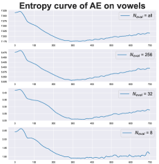
Figure A5: The loss entropy curves of the training process of AE on the vowels dataset with varying $N_{eval}$ values.

The comparison of the AUC distribution of the Naive, Optimal, and Entropy across varing HP configurations and models are shown in Fig A6.

Figure A5 displays the loss entropy curve of the AE training process on the vowels dataset with varying $N_{eval}$ values. The correlation between these entropy curves and the original entropy curve computed on the entire dataset is demonstrated in Figure 6 (b) of our primary paper. The results indicate that even with a small $N_{eval}$ (e.g., 8), the loss entropy curve remains quite similar to the entropy curve obtained by a larger $N_{eval}$.

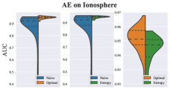
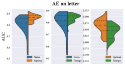
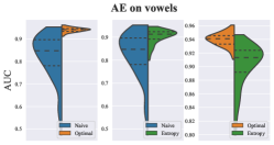
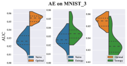
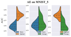
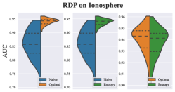
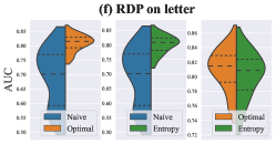
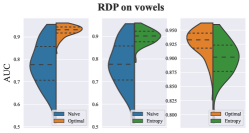
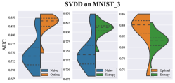
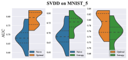
Figure A6: Comparison of AUC distribution of Naive, Optimal, and Entropy across varing HP configurations.

References

- [1] Aggarwal, C. C., and Sathe, S. Theoretical foundations and algorithms for outlier ensembles. Acm sigkdd explorations newsletter 17, 1 (2015), 24–47.
- [2] Baldi, P. Autoencoders, unsupervised learning, and deep architectures. In Proceedings of ICML workshop on unsupervised and transfer learning (2012), JMLR Workshop and Conference Proceedings, pp. 37–49.
- [3] Breunig, M. M., Kriegel, H.-P., Ng, R. T., and Sander, J. Lof: identifying density-based local outliers. In Proceedings of the 2000 ACM SIGMOD international conference on Management of data (2000), pp. 93–104.
- [4] Campos, G. O., Zimek, A., Sander, J., Campello, R. J., Micenková, B., Schubert, E., Assent, I., and Houle, M. E. On the evaluation of unsupervised outlier detection: measures, datasets, and an empirical study. Data mining and knowledge discovery 30, 4 (2016), 891–927.
- [5] Chalapathy, R., and Chawla, S. Deep learning for anomaly detection: A survey. arXiv preprint arXiv:1901.03407 (2019).
- [6] Chandola, V., Banerjee, A., and Kumar, V. Anomaly detection: A survey. ACM computing surveys (CSUR) 41, 3 (2009), 1–58.
- [7] Chen, J., Sathe, S., Aggarwal, C., and Turaga, D. Outlier detection with autoencoder ensembles. In Proceedings of the 2017 SIAM international conference on data mining (2017), SIAM, pp. 90–98.
- [8] Ding, X., Zhao, L., and Akoglu, L. Hyperparameter sensitivity in deep outlier detection: Analysis and a scalable hyper-ensemble solution. arXiv preprint arXiv:2206.07647 (2022).
- [9] Dou, Y., Liu, Z., Sun, L., Deng, Y., Peng, H., and Yu, P. S. Enhancing graph neural network-based fraud detectors against camouflaged fraudsters. In Proceedings of the 29th ACM International Conference on Information & Knowledge Management (2020), pp. 315–324.
- [10] Goix, N. How to evaluate the quality of unsupervised anomaly detection algorithms? arXiv preprint arXiv:1607.01152 (2016).
- [11] Goldstein, M., and Uchida, S. A comparative evaluation of unsupervised anomaly detection algorithms for multivariate data. PloS one 11, 4 (2016), e0152173.
- [12] Han, S., Hu, X., Huang, H., Jiang, M., and Zhao, Y. Adbench: Anomaly detection benchmark. arXiv preprint arXiv:2206.09426 (2022).
- [13] Hawkins, D. M. Identification of outliers, vol. 11. Springer, 1980.
- [14] Hojjati, H., Ho, T. K. K., and Armanfard, N. Self-supervised anomaly detection: A survey and outlook. arXiv preprint arXiv:2205.05173 (2022).
- [15] Hosmer, D. W., Lemeshow, S., and Sturdivant, R. Area under the receiver operating characteristic curve. Applied Logistic Regression. Third ed: Wiley (2013), 173–182.
- [16] Huang, H., Qin, H., Yoo, S., and Yu, D. Physics-based anomaly detection defined on manifold space. ACM Transactions on Knowledge Discovery from Data (TKDD) 9, 2 (2014), 1–39.
- [17] Kiran, B. R., Thomas, D. M., and Parakkal, R. An overview of deep learning based methods for unsupervised and semi-supervised anomaly detection in videos. Journal of Imaging 4, 2 (2018), 36.
- [18] Lai, K.-H., Zha, D., Xu, J., Zhao, Y., Wang, G., and Hu, X. Revisiting time series outlier detection: Definitions and benchmarks. In Thirty-fifth Conference on Neural Information Processing Systems Datasets and Benchmarks Track (Round 1) (2021).
- [19] LeCun, Y., Bottou, L., Bengio, Y., and Haffner, P. Gradient-based learning applied to document recognition. Proceedings of the IEEE 86, 11 (1998), 2278–2324.
- [20] Lee, M.-C., Shekhar, S., Faloutsos, C., Hutson, T. N., and Iasemidis, L. Gen 2 out: Detecting and ranking generalized anomalies. In 2021 IEEE International Conference on Big Data (Big Data) (2021), IEEE, pp. 801–811.
- [21] Lin, Z., Thekumparampil, K., Fanti, G., and Oh, S. Infogan-cr and modelcentrality: Self-supervised model training and selection for disentangling gans. In international conference on machine learning (2020), PMLR, pp. 6127–6139.
- [22] Liu, B., Tan, P.-N., and Zhou, J. Unsupervised anomaly detection by robust density estimation. In Proceedings of the AAAI Conference on Artificial Intelligence (2022), vol. 36, pp. 4101–4108.
- [23] Liu, F. T., Ting, K. M., and Zhou, Z.-H. Isolation forest. In 2008 eighth ieee international conference on data mining (2008), IEEE, pp. 413–422.
- [24] Liu, K., Dou, Y., Zhao, Y., Ding, X., Hu, X., Zhang, R., Ding, K., Chen, C., Peng, H., Shu, K., et al. Bond: Benchmarking unsupervised outlier node detection on static attributed graphs. In Thirty-sixth Conference on Neural Information Processing Systems Datasets and Benchmarks Track (2022).
- [25] Liu, Y., Li, Z., Zhou, C., Jiang, Y., Sun, J., Wang, M., and He, X. Generative adversarial active learning for unsupervised outlier detection. IEEE Transactions on Knowledge and Data Engineering 32, 8 (2019), 1517–1528.
- [26] Ma, M. Q., Zhao, Y., Zhang, X., and Akoglu, L. The need for unsupervised outlier model selection: A review and evaluation of internal evaluation strategies. ACM SIGKDD Explorations Newsletter 25, 1 (2023).
- [27] Marques, H. O., Campello, R. J., Sander, J., and Zimek, A. Internal evaluation of unsupervised outlier detection. ACM Transactions on Knowledge Discovery from Data (TKDD) 14, 4 (2020), 1–42.
- [28] Nguyen, T. T., Nguyen, U. Q., et al. An evaluation method for unsupervised anomaly detection algorithms. Journal of Computer Science and Cybernetics 32, 3 (2016), 259–272.
- [29] Nguyen, T. T., Nguyen, U. Q., et al. An evaluation method for unsupervised anomaly detection algorithms. Journal of Computer Science and Cybernetics 32, 3 (2016), 259–272.
- [30] Pang, G., Shen, C., Cao, L., and Hengel, A. V. D. Deep learning for anomaly detection: A review. ACM Computing Surveys (CSUR) 54, 2 (2021), 1–38.
- [31] Qiu, C., Pfrommer, T., Kloft, M., Mandt, S., and Rudolph, M. Neural transformation learning for deep anomaly detection beyond images. In International Conference on Machine Learning (2021), PMLR, pp. 8703–8714.
- [32] Ruff, L., Kauffmann, J. R., Vandermeulen, R. A., Montavon, G., Samek, W., Kloft, M., Dietterich, T. G., and Müller, K.-R. A unifying review of deep and shallow anomaly detection. Proceedings of the IEEE 109, 5 (2021), 756–795.
- [33] Ruff, L., Vandermeulen, R., Goernitz, N., Deecke, L., Siddiqui, S. A., Binder, A., Müller, E., and Kloft, M. Deep one-class classification. In International conference on machine learning (2018), PMLR, pp. 4393–4402.
- [34] Schlegl, T., Seeböck, P., Waldstein, S. M., Schmidt-Erfurth, U., and Langs, G. Unsupervised anomaly detection with generative adversarial networks to guide marker discovery. In International conference on information processing in medical imaging (2017), Springer, pp. 146–157.
- [35] Song, H., Li, P., and Liu, H. Deep clustering based fair outlier detection. In Proceedings of the 27th ACM SIGKDD Conference on Knowledge Discovery & Data Mining (2021), pp. 1481–1489.
- [36] Steinbuss, G., and Böhm, K. Benchmarking unsupervised outlier detection with realistic synthetic data. ACM Transactions on Knowledge Discovery from Data (TKDD) 15, 4 (2021), 1–20.
- [37] Thomas, M., and Joy, A. T. Elements of information theory. Wiley-Interscience, 2006.
- [38] Voulodimos, A., Doulamis, N., Doulamis, A., Protopapadakis, E., et al. Deep learning for computer vision: A brief review. Computational intelligence and neuroscience 2018 (2018).
- [39] Wang, H., Pang, G., Shen, C., and Ma, C. Unsupervised representation learning by predicting random distances. arXiv preprint arXiv:1912.12186 (2019).
- [40] Wang, S., Zeng, Y., Liu, X., Zhu, E., Yin, J., Xu, C., and Kloft, M. Effective end-to-end unsupervised outlier detection via inlier priority of discriminative network. Advances in neural information processing systems 32 (2019).
- [41] Weller-Fahy, D. J., Borghetti, B. J., and Sodemann, A. A. A survey of distance and similarity measures used within network intrusion anomaly detection. IEEE Communications Surveys & Tutorials 17, 1 (2014), 70–91.
- [42] Wu, Z., Pan, S., Chen, F., Long, G., Zhang, C., and Philip, S. Y. A comprehensive survey on graph neural networks. IEEE transactions on neural networks and learning systems 32, 1 (2020), 4–24.
- [43] Xia, Y., Cao, X., Wen, F., Hua, G., and Sun, J. Learning discriminative reconstructions for unsupervised outlier removal. In Proceedings of the IEEE International Conference on Computer Vision (2015), pp. 1511–1519.
- [44] Zhao, Y., Nasrullah, Z., and Li, Z. Pyod: A python toolbox for scalable outlier detection. arXiv preprint arXiv:1901.01588 (2019).
- [45] Zhao, Y., Rossi, R., and Akoglu, L. Automatic unsupervised outlier model selection. Advances in Neural Information Processing Systems 34 (2021), 4489–4502.