Real-Time Scheduling for Time-Sensitive Networking: A Systematic Review and Experimental Study

Abstract

Time-Sensitive Networking (TSN) has been recognized as one of the key enabling technologies for Industry 4.0 and has been deployed in many mission- and safety-critical applications e.g., automotive and aerospace systems. Given the stringent real-time requirements of these applications, the Time-Aware Shaper (TAS) draws special attention among TSN’s many traffic shapers due to its ability to achieve deterministic timing guarantees. Several scheduling methods for TAS shapers have been recently developed that claim to improve system schedulability. However, these scheduling methods have yet to be thoroughly evaluated, especially through experimental comparisons, to provide a systematical understanding on their performance using different evaluation metrics in diverse application scenarios. In this paper, we fill this gap by presenting a systematic review and experimental study on existing TAS-based scheduling methods for TSN. We first categorize the system models employed in these works along with the specific problems they aim to solve, and outline the fundamental considerations in the designs of TAS-based scheduling methods. We then perform an extensive evaluation on seventeen representative solutions using both high-fidelity simulations and a real-life TSN testbed, and compare their performance under both synthetic scenarios and real-life industrial use cases. Through these experimental studies, we identify the limitations of individual scheduling methods and highlight several important findings. We expect this work will provide foundational knowledge and performance benchmarks needed for future studies on real-time TSN scheduling, and thus have a significant impact to the community.

I Introduction

Time-Sensitive Networking (TSN), as an enhancement of Ethernet, has quickly become the local area network (LAN) technology of choice for enabling the coexistence of information technology (IT) and operation technology (OT) in the industrial Internet-of-Things (IIoT) paradigm. TSN aims to provide deterministic communications between Layer-2 networks which is highly desirable for many real-time industrial applications, such as process automation and factory automation [1, 2]. To enable such communication capabilities, the TSN Task Group has developed a suite of traffic shapers in the TSN standards, including the Credit-Based Shaper (CBS) [3], Asynchronous Traffic Shaper (ATS) [4], and Time-Aware Shaper (TAS) [5], to handle different traffic types and satisfy real-time communication requirements at different levels. In terms of providing strict real-time performance guarantees, the TAS stands out by leveraging network-wide synchronization and time-triggered scheduling mechanisms [6, 7], making it a critical technology to supporting deterministic traffic in industrial applications.

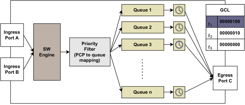
Figure 1: An illustration of the Time-Aware Shaper (TAS) mechanism in a Time-Sensitive Networking (TSN) bridge.

TAS operates in a time-triggered scheduling fashion, which achieves deterministic communications by buffering and releasing traffic at specific time instances following a predetermined schedule. Specifically, as shown in Fig. 1, each egress port in a TSN switch, also called a bridge, is equipped with a set of time-gated queues for buffering frames from each traffic flow. A scheduled gate mechanism is utilized to open or close individual queues and control the transmission of frames according to a predefined Gate Control List (GCL). Each GCL includes a limited number of entries. Each entry provides the status of associated queues over a particular duration. The GCL repeats itself periodically, and the period is called cycle time. The network-wide schedule is generated by Centralized Network Configuration (CNC) and deployed on individual TSN bridges. In addition to the scheduled gate, the priority filter utilizes a 3-bit Priority Code Point (PCP) field in the packet header to identify the stream priority, and directs incoming traffic to the appropriate egress queue according to the priority-to-queue mapping. It is worth noting that this mapping may vary across different bridges, making the same traffic be assigned to different queues on the bridges along its routing path [5].

Although the scheduling mechanism of TAS is clearly defined in the IEEE 802.1Qbv standard, the configuration of TAS, e.g., what to put in the GCL and how to assign queues for individual traffic at each hop, has no clear-cut best practice. Specifically, the fundamental question underlying TAS-based real-time scheduling in TSN is how to generate a network-wide schedule to guarantee the timing requirements of all time-triggered (TT) traffic [8]. Given that industrial applications that employ TAS-based TSN as the communication fabric can be diverse from many different perspectives (e.g., traffic patterns, QoS requirements, network topology, and deployment environments), the specific scheduling problem to be studied may vary significantly. This results in a large amount of research efforts from researchers and practitioners to study various system models and develop corresponding algorithms to address specific TAS-based TSN scheduling problems. These studies considerably enrich the TSN literature, paving the way to improve TSN network performance.

There have been several recent survey works in the literature on real-time scheduling in TSN networks. (e.g., [8, 7, 9, 10, 11, 12]). These studies provided a broad overview of the TSN standards, identified the limitations of the existing TSN scheduling methods, and outlined future research directions to address these limitations. In addition, [13, 8] provided comparisons among various TSN scheduling approaches, with [8] primarily focusing on TAS-based studies and [13] extending the comparison to all TSN shapers. However, all the aforementioned works have been either on a review basis or only performed conceptual comparisons among the existing solutions, which is not sufficient for determining the effectiveness of individual methods under diverse scenarios.

To fill this gap, this paper presents comprehensive experiment designs and quantitative performance comparison among 17 representative time-triggered scheduling methods proposed for TSN since 2016 (i.e., [14, 15, 16, 17, 18, 19, 20, 21, 22, 23, 24, 25, 26, 27, 28, 29]). We conducted a thorough experimental study by considering various key experiment settings, including both stream set and network settings in synthetic scenarios. In addition, we analyzed the impact of the aforementioned settings on the performance of the scheduling methods, using multi-dimensional metrics to assess feasibility, scalability, and the quality of solutions. Our study shows that there is no one-size-fits-all solution on schedulability, as no single method outperforms others in all scenarios. Furthermore, we demonstrate that diverse experiment settings significantly complicate the fair evaluation of scheduling methods without introducing bias, which could result in previous research conclusions that are valid only in specific settings. We expect that our findings will help the community understand the benefits and drawbacks of existing TSN scheduling methods and provide valuable insights for the development of future TSN scheduling methods.

In summary, this work makes the following contributions:

1. We provide a comprehensive up-to-date review of TAS-based real-time scheduling methods for TSN, and outline the fundamental considerations in the designs of TAS-based scheduling methods.

2. We set up a comprehensive hardware testbed to quantitatively measure the commonly used parameters in TSN real-time scheduling models, and validate the correctness of TSN scheduling methods through the testbed.

3. We perform an extensive evaluation on 17 representative TAS-based scheduling methods, and compare their performance using metrics that are of interest to the industry in comprehensive scenarios.

4. We summarize the findings from our performance evaluation that can provide insights for future research and development on TSN real-time scheduling methods.

The remainder of this paper is structured as follows. Section II presents the fundamental concepts and system models used in the literature for real-time scheduling in TSN. Section III provides a classification of existing scheduling methods and introduces the key ideas underlying their algorithm designs. Section IV shows our testbed validation results for the commonly used model parameters. Section V describes our simulation-based experimental settings. Section VI presents the experimental results and discusses the significant findings from our study. Section VII provides the takeaway lessons of this study. Finally, Section VIII concludes the paper and discusses future work.

II Background and System Model

This section presents an overview of the network models, traffic models, and scheduling models for real-time traffic scheduling in TSN. It provides the foundation for the discussion of the TAS-based scheduling methods in Section III.

II-A Network Models

A TSN network consists of two types of devices: bridges and end stations (ES). A bridge can forward Ethernet frames for one or multiple TSN streams according to a schedule constructed based on the IEEE 802.1Q standard. Each ES can be a talker, acting as the source of TSN stream(s), a listener, acting as the destination of TSN stream(s), or both.

Each full-duplex physical link connecting two TSN devices (either bridge or ES) is modeled as two directed logical links. Each logical link is associated with the following four attributes, which are determined by the capacity of the bridge or ES connected by the link:

•  Propagation delay refers to the time duration of a signal transmitting on the physical link (i.e., Ethernet cable). This delay is solely dependent on the length of the cable and the type of physical media used.

•  Line rate refers to the data rate that frames can be transmitted over a logical link within a given time interval. There are three line rates commonly employed for TSN (10/100/1000 Mbps), while higher-speed TSN bridges with 10/100 Gbps line rates have also been developed recently.

•  Number of egress queues refers to the available egress queues dedicated to TT traffic. The IEEE 802.1Q standard sets a max of eight queues per egress port for a TSN bridge [30].

•  Maximum GCL length indicates the maximum allowed number of entries in the Gate Control List (GCL) of a logical link. It is set between 8 and 1024 for typical TSN bridges [15].

In addition to the above attributes associated with logical links, TSN also has network-wide attributes that are shared across all nodes and links, such as the synchronization error:

•  Synchronization error is defined as the maximum time offset between any two non-faulty logical clocks in the network.

In TSN networks, a stream refers to a unidirectional flow of data transmitted from a single talker to one or multiple listeners, passing through bridges over multiple logical links. For example, in Fig. 2, there are four streams transmitting in a TSN network that comprises 5 bridges and 5 ESs. In addition to time-triggered traffic, TSN can also accommodate lower-criticality asynchronous traffic, such as standard Ethernet and audio and video (AVB) traffic. Driven by the determinism requirements posed by real-time industrial applications, the literature mainly focuses on the TT traffic scheduling problem, which is also the emphasis of this paper.

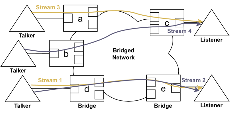
Figure 2: An example TSN network comprising 5 bridges and 5 end stations (ES) with $4$ streams deployed in the network.

II-B Traffic Models

Each TSN stream can be characterized by five parameters: release time, period, payload size, deadline, and jitter. Each of these parameters can be modeled individually in order to capture the specific characteristics of the targeted traffic type, based on the application scenario under study. Using different traffic models can lead to different scheduling results and network performance.

•  Release time: The release time of a stream is defined as the time instance when its first frame is dispatched on the physical link by the talker. Depending on whether the talker is able to determine the release time of its stream(s), the traffic model can be classified into fully schedulable traffic and partially schedulable traffic. The fully schedulable traffic model allows the scheduler to configure the release time of each stream and thus yield higher schedulability. It, however, might incur increased scheduling complexity compared to the partially schedulable traffic model.

•  Period: The period of a stream determines the inter-arrival pattern of its frames. It can be classified into strictly periodic and non-strictly periodic model based on the determinism of their arrival times. In a strictly periodic model, each frame follows the same release offset, resulting in a fixed time interval between any two consecutive frames when they are released by the talker. By contrast, in the non-strictly periodic model, frames from the same stream can be released with varied but bounded offsets.

•  Payload size: Payload size refers to the size of the application data to be transmitted within a stream. When the payload size is larger than 1500 bytes, a stream may compromise multiple frames in the same period.

There are two main strategies for transmitting multiple frames from the same stream in the same period. The first approach schedules each frame individually while preserving the frame order of the same stream by introducing additional constraints. Alternatively, the second approach schedules all frames from the same stream successively within an extended time duration on each link.

•  Deadline: The deadline of a stream defines the time by which the frame must be received at the listener, such that the release time from the talker plus the end-to-end delay does not exceed this deadline. The deadline of a stream can be modeled as implicit (equal to the period), constrained (less than the period), or arbitrary, according to the application scenario. Note that, under the arbitrary deadline model, a frame released in its period can be scheduled into the next period interval and such cases should be carefully handled in the scheduling method to avoid potential conflicts.

•  Jitter: The jitter captures the variation of end-to-end stream delay (i.e., the difference between the minimum and maximum delays of frames transmitted from the same stream), following the definition in IEC/IEEE 60802 TSN Profile [31]. The zero-jitter model enforces fully deterministic traffic behavior for each frame, whereas the jitter-allowed model permits limited conflicts from other traffic on delay, subject to a user-defined jitter upper bound. Fig.3(a) illustrates a jitter-allowed scheduling example for stream S1, with a delay of 6 for the first instance and 12 for the second. Fig.3(b) demonstrates how jitter arises from interference when both S1 and S2 share a GCL entry along the path, resulting in a bounded delay between 10 and 12.

II-C Scheduling Models

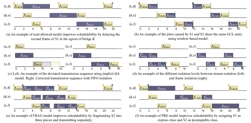
Figure 3: An illustration of various scheduling models applied on the example in Fig. 2. $f_{i,k,a,b}$ indicates the $k$-th frame of stream-$i$ scheduled on link $(a,b)$, $f_{i,k,a,b}^{r}$ indicates the $r$-th fragment if fragmentation or preemption is applied. To simplify the notations, we use $t$ to denote the talker and $l$ to denote the listener associated with each path. The up arrow indicates the frame release time at the talker and the down arrow indicates the frame reception time at the listener. Solid area indicates the actual transmission pattern and shallow area indicates the traffic planning result. The dash line indicates the border of a GCL entry.

Based on the network and traffic models described above, the TAS-based real-time scheduling problem in TSN aims to construct feasible communication schedules (assignment of transmission times for each stream on involved bridges) to satisfy the temporal constraints imposed by the streams deployed in the TSN network. For this aim, a range of scheduling models have been proposed to define the constraints made on end-to-end delay, jitter, queuing assignment, routing path, fragmentation, and preemption. In this section, we summarize these scheduling models and categorize them according to their unique features.

•  Models based on Queuing Delay: The end-to-end delay of a frame is defined as the duration between the time when the frame is released at the talker and the time when the entire frame is received by the listener. This delay consists of four parts: processing delay, propagation delay, transmission delay, and queuing delay. In TSN, the propagation and processing delays are typically considered constant [20]. The transmission delay depends on the payload size and the line rate of the link. The queuing delay refers to the amount of time that a frame spends waiting in the queue. Based on different assumptions on the queuing delay, the scheduling models can be classified as the no-wait and wait-allowed models. The no-wait scheduling model requires consecutive frame transmissions along the path, i.e., frames should be forwarded without queuing delay. As a result, the no-wait scheduling model focuses on planning the release times of the streams on the talkers, which typically results in reduced scheduling effort but smaller solution spaces. On the other hand, the wait-allowed scheduling model is more general as it allows frames to be stored in the queue and forwarded at a later time on bridges, therefore having a larger solution space. For example, Fig. 3(a) follows the wait-allowed scheduling model as the second frame from stream S1 waits 2 time units on link $(d,e)$ and 4 time units on link $(e,l)$. The no-wait scheduling model cannot find a feasible solution in this case.

•  Models based on Scheduling Entity: The scheduling models can be classified into frame-based, window-based and class-based models depending on the objects used in the scheduling methods for the allocation of GCL entry [7]. The frame-based model schedules the transmission time of each frame in a per-stream fashion and directly maps it to a dedicated GCL entry. By constraining that no overlap exists for any two frames’ transmission time, the frame-based model guarantees that there is no interference between any two streams. The window-based model partitions frames into different groups and jointly schedules the transmission time of the frames in each group. As each GCL entry is shared by a group of frames, the transmission order of each frame can be interfered by other frames within the same group and results in jitter. For example, in Fig. 3(b), streams S1 and S2 are assigned to the same egress queue and share the same GCL entry according to a window-based scheduling model. Their transmission orders in two consecutive periods are different within the window which causes jitter. It is worth noting that in the window-based scheduling model, the large inter-dependencies between the window allocation and traffic grouping may pose significant runtime and memory overhead [26]. The class-based scheduling model allocates resources for each traffic class and guarantees the same deadline and jitter requirements for a whole class. Each traffic class is mapped to a dedicated egress queue. Because the class-based model is mainly employed for asynchronous traffic classes (e.g., AVB and BE traffic), it is out of the scope and not discussed in this paper [32].

•  Models based on Queue Assignment (QA): Based on how the frames are assigned to the egress queue(s), the scheduling models can be classified into unrestricted QA models and explicit QA models. The unrestricted QA models are derived from TTEthernet scheduling methods, which assume a global schedule that defines the temporal behavior of all frames without considering queuing assignment [33]. However, the unrestricted QA models cannot be directly applied to TSN, as ignoring QA may violate the FIFO property of TSN queues and result in deviations in actual transmission time from the designed schedule. For instance, as shown in Fig. 3(c), the schedule on the left is valid under the unrestricted QA model where two streams are forwarded simultaneously at their first hop. Stream S4 is scheduled earlier than S3 on link $(c,l)$ without any conflicts. However, if both streams are assigned to the same queue, S3’s frame will use the transmission slot allocated to S4 during run time, causing S4 to be suspended and miss its deadline. Please note that this inconsistency only happens under the wait-allowed model, since the no-wait model forwards frames immediately without queuing.

To avoid such schedule inconsistency, explicit QA models isolate streams into different queues by jointly computing the queue assignment along with the schedule. For this aim, several isolation constraints are proposed which can be categorized into three levels: FIFO, frame-based, and stream-based isolation. The basic idea of FIFO isolation is to prevent reordering the forwarding sequence of frames when they are assigned to the same queue. For instance, the schedule on the right side of Fig. 3(c) enforces stream S4 to arrive earlier than S3, so that the forwarding order matches the predefined schedule, even if they are within the same queue.

Frame-based isolation and stream-based isolation are comparatively more realistic as they take into account frame loss, unbounded processing jitter, and interleaving caused by fragmentation when the payload size is larger than the MTU. For example, as shown on the right of Fig. 3(c), under the FIFO isolation model, stream S3 will forward earlier than expected by using the slot allocated for S4 on link $(c,l)$ if the frame of S4 is lost. Frame-based isolation ensures that at one time, only one frame can exist in the queue so that it is not interfered by other frames’ fault conditions. For example, as illustrated on the right side of Fig. 3(d), the frame of stream S3 can only arrive at link $(c,l)$ after the first fragment of stream S4 is dispatched. The second fragment of S4 can only arrive at link $(c,l)$ after the frame of S3 is dispatched. Compared to frame-based isolation, stream-based isolation is more stringent. It requires that the frame of the current stream can only be enqueued after all frames of the previous stream(s) have been fully dispatched, as shown on the left side of Fig. 3(d). The frame of S3 must wait until all the fragments of S4 are dispatched. It is suggested that frame-based isolation provides more flexibility but takes more time to construct the schedule compared to the stream-based model [14].

•  Models based on Routing and Scheduling Co-Design: Scheduling models can be further categorized as fixed routing (FR) model and joint routing and scheduling (JRS) model. The JRS model allows the co-design of route selection and schedule construction, while the FR model focuses on schedule construction only, assuming that the routes are pre-determined. By optimizing the routing and scheduling decisions in a joint fashion, the JRS model could offer better resource utilization and schedulability in general when compared to the FR model. However, the JRS model may also incur much higher computational overheads and may not be able to find feasible solutions if the computing resource is constrained.

•  Models based on Fragmentation: In the network layer, fragmentation occurs when a packet is split into smaller fragments to fit the MTU size of the network. However, default fragmentation may result in high latency due to the large fragment size. To address this issue, the fragmentation (FRAG) model is proposed, which determines the number and size of fragments along with the schedule construction. The FRAG model, to some extent, can improve schedulability, especially in cases when the deadline is exceeded due to the large frame size. Fragmenting a large frame into multiple fragments may reduce the transmission delay, as each fragment can be transmitted separately, eliminating the need to wait for the entire frame to be fully received before forwarding it to the next hop. For example, if we consider stream S2 in Fig. 3(e) with a transmission duration of 6 time units, the minimum end-to-end delay for a frame of S2 to travel through the three hops is 18 time units. However, the FRAG model fragments the original frame into three small fragments, forwarding can start immediately after the first fragment is received on each hop. In this scenario, if the deadline is set to 12, S2 can only be scheduled for transmission under the FRAG model. It is important to note that fragmentation comes with extra header overhead, which may negatively impact the link utilization.

•  Models based on Preemption: The IEEE 802.1Qbu standard defines frame preemption as the capacity of an express frame to interrupt the transmission of a preemptable frame and subsequently resume the preempted frame at the earliest available opportunity. Frames may be assigned with varied preemption classes at different hops, with only express frames being able to interrupt preemptable frames. The preemptable frame can thus be broken into two or more fragments. For instance, in Fig. 3(f), the frame of stream S2 on link $(d,e)$ is designated as a preemptable class and is consequently preempted by the frame of S1, classified as an express class, at time 12 during the transmission. Following the completion of stream S1’s transmission, the second fragment of S2 resumes its transmission. It is worth noting that the preemption (PRE) model does not reduce the transmission delay compared to FRAG, as frames can only be forwarded after all fragments are fully received and reassembled. For example, in Fig. 3(f), link $(e,l)$ cannot forward at time 12 when the first fragment is received but has to wait until time 16 when both fragments have been received. Nonetheless, if preemption is disabled, S1 fails to meet its deadline, resulting in an unschedulable stream set. In addition, as fragmentation only occurs when necessary, the PRE model offers better bandwidth conservation when compared to the FRAG model due to the reduced number of generated headers. For example, there is only one additional header created for the second fragment of the frame of S2 along its path in Fig. 3(f). By contrast, a total number of six headers are generated under the FRAG model in Fig. 3(e).

III Real-Time Scheduling Methods for TSN

Figure 4: Classification of the TSN real-time scheduling methods based on the employed system models.

This section provides a comprehensive review of 17 representative TAS-based real-time scheduling methods in TSN published since 2016. Those scheduling methods aim to find a feasible network-wide configuration, including routing paths and schedules, meeting the end-to-end timing requirements of a given set of streams. Additionally, each method has its unique focus, such as enhancing schedulability, boosting scalability, or reducing GCL length. We categorize them based on their employed system models and proposed scheduling algorithms (see Fig. 4).

We first classify all the selected work into FR or JRS methods based on whether the routing paths of individual streams are pre-determined or jointly selected when constructing the schedule. The methods in each group are then further divided into no-wait and wait-allowed methods based on their employed delay models. Finally, we categorize each method into either exact or heuristic solutions based on whether the method can yield an optimal schedule or not. Please note that some selected works proposed both exact and heuristic solutions, but in this paper, we only evaluate one of them based on their key contributions to make the review and performance comparison more concise and informative.

We have selected these methods based on two main criteria: 1) Breadth: to give a comprehensive experimental study, we aim to include as diverse a set of models and algorithms as possible; 2) Relevance: to concentrate on real-time scheduling of time-triggered traffic in TSN, approaches centered on non-real-time scenarios or those aiming to enhance AVB or BE traffics in mixed-criticality scenarios or improve reliability are not included. We have also excluded those learning-based methods that cannot provide a deterministic schedule.

III-A Fixed Routing (FR) Methods

FR methods assume that the routing paths of individual streams are pre-determined and provided as input for the scheduling algorithms. Based on the IEEE 802.1Qca standard, the default routing paths generated by the Shortest Path Bridging Protocol ensure that all streams are routed along their shortest paths between the talkers and listeners [34].

III-A1 No-wait

The no-wait scheduling model requires that frames are forwarded along its routing path without queuing delay. Among the 17 real-time scheduling methods that we examine in this paper, three methods employ a combination of the FR and no-wait model. They focus on minimizing the end-to-end latency based on the predetermined routing paths.

•  SMT-NW: Durr et al.[20] addressed the crucial problem of reducing the end-to-end latency of TT traffic and increasing the available bandwidth for BE traffic. The key idea is to adapt this problem to the no-wait job-shop scheduling problem[35]. The authors proposed an exact solution using the CPLEX Integer Linear Programming (ILP) solver with Big-M logical expressions and a compression algorithm in post-processing to minimize the guard bands to save the bandwidth. To tackle the scalability issue, a heuristic approach based on Tabu search was also proposed.

•  SMT-FRAG: Jin et al. [23] proposed a no-wait scheduling approach for improving schedulability by introducing a joint scheduling with fragmentation framework. The key idea is to jointly determine the number and size of fragments for individual streams during the schedule construction. The scheduling problem was formalized using a Satisfiability Modulo Theories (SMT) formulation and solved using the Z3 solver. To address the scalability issue, the authors also proposed a heuristic solution based on fixed-priority scheduling.

•  DT: Zhang et al. [36] addressed the high computational overhead issue associated with the non-overlap constraint checking during the scheduling process. The authors proposed a stream-aware model conversion algorithm that accelerates the scheduling process for the zero-jitter model. It employed the divisibility theory to detect collision and speeded up this process by only comparing the first instances of two streams. In addition, this work introduced an efficient incremental searching strategy without traceback, further reducing the runtime overhead.

III-A2 Wait-allowed

In the wait-allowed scheduling model, frames can be stored in the egress queue and forwarded at a later time. It thus has a larger solution space compared with that of the no-wait scheduling model. We evaluate the following seven works that employ a combination of the FR and wait-allowed model to solve the real-time scheduling problem in TSN.

•  SMT-WA: Craciunas et al. [14] focused on providing accurate modeling for the behavior of TAS-based scheduling mechanisms in wait-allowed scenarios. They first formalized the constraints for constructing valid schedules using SMT formulation based on the wait-allowed model. To ensure correctness, a key contribution of their work is to first introduce the queuing isolation model such as frame- and stream-based isolation in the TSN field.

•  AT: Oliver et al. [15] addressed the challenge that GCLs only support a limited number of entries in practical implementations. Their study introduced a window-based scheduling method that applied array theory to an SMT solver, taking the maximum number of GCL entries as the algorithm input. In addition, this work incorporated the queue assignment and isolation model into the solution.

•  I-OMT: Jin et al. [26] also addressed the practical limitation of GCL length. Instead of setting a hard constraint on the GCL length, this work minimized the GCL length by proposing an iterative-Optimization Modulo Theories (OMT)-based approach to scheduling streams by group. The queue assignment is calculated for each stream based on its payload size, shortest routing path, and deadline. Then it is taken as the input of the iterative OMT solver. The stream-based isolation is formulated as a constraint to guarantee the correctness of the queue assignment.

•  CP-WA: Vlk et al.[25] focused on modeling deterministic TT traffic through constraint programming (CP). CP provides a more efficient solution to the TSN real-time scheduling problem with an All-different Constraint compared to other formalization such as SMT and ILP. This work also proposed a decomposition optimization to enhance scalability, which alternated between routing and scheduling searches.

•  SMT-PRE: Zhou et al. [27] aimed to increase schedulability by integrating the preemption feature from the IEEE 802.1Qbu standard [37]. An SMT-based approach was proposed to assign streams to express class and preemptable class while jointly determining the schedule. The allowed maximum number of preempted fragments is taken as the algorithm input.

•  LS-TB: Vlk et al. [21] addressed the challenge of poor scalability in scheduling large-scale TT traffic in TSN, an inherent problem when using general third-party solvers. Their proposed scheduler can revert to a previous search stage and modify the timing and queue assignment if the current frame conflicts with any other scheduled frames. The authors utilized two data structures, the global and local conflict sets, to decide the search order.

•  LS-PL: Bujosa et al. [29] focused on improving scalability in scheduling large-scale TT traffic in TSN. The authors proposed a heuristic algorithm that allocates links into phases based on their dependency and then schedules these links phase by phase. The algorithm also determines the queue assignment during the heuristic search. This work covered both the no-wait and wait-allowed model, offering flexible jitter control under different scenarios.

TABLE I: A summary of the system models and scheduling approaches in the studied TSN scheduling methods.

Article

Year

Fully schedulable

Strictly periodic

No-wait

Window -based

Queueing

Routing

Multicast

Heuristic

Exact

Algorithms

Enhancements

Craciunas et al. (SMT-WA)

2016

✓

✓

✓

✓

SMT

Dürr et al. (SMT-NW)

2016

✓

✓

✓

(✓)

✓

ILP (Tabu)

Schweissguth et al. (JRS-WA)

2017

✓

✓

✓

✓

ILP

Paths reduce

Oliver et al. (AT)

2018

✓

✓

✓

✓

SMT

Array-theory

Falk et al. (JRS-NW-L)

2018

✓

✓

✓

✓

✓

ILP

Logic indicator

Pahlevan et al. (LS)

2019

✓

✓

✓

✓

✓

List scheduler

Schweissguth et al. (JRS-MC)

2020

✓

✓

✓

✓

✓

ILP

Paths reduce

Atallah et al. (I-ILP)

2020

✓

✓

✓

✓

✓

✓

Iterative-ILP

Xi et al. (I-OMT)

2020

✓

✓

✓

(✓)

Iterative-OMT

Falk et al. (CG)

2020

✓

✓

✓

✓

✓

(✓)

Conflict-graph

Hellmanns et al. (JRS-NW)

2021

✓

✓

✓

✓

✓

ILP

Path cut-off

Jin et al. (SMT-FRAG)

2021

✓

✓

✓

(✓)

✓

SMT (WCRT)

Fragmentation

Vlk et al. (CP-WA)

2021

✓

✓

✓

(✓)

✓

CP (Decompose)

Vlk et al. (LS-TB)

2022

✓

✓

✓

(✓)

List scheduler

Traceback

Bujosa et al. (LS-PL)

2022

✓

✓

✓

List scheduler

Per-link search

Zhou et al. (SMT-PRE)

2022

✓

✓

SMT

Preemption

Zhang et al. (DT)

2022

✓

✓

✓

✓

(✓)

Divisibility

III-B Joint Routing and Scheduling (JRS) Methods

A feasible schedule may not be found when the routing paths of the streams are pre-determined under the FR model. By contrast, the JRS-based methods allow the scheduler to jointly decide the routes and schedules for each stream, thus providing opportunities to offer better network resource utilization and schedulability.

III-B1 No-wait

The following works study the TSN scheduling problem using a combination of JRS and no-wait model.

•  JRS-NW-L: Falk et al. [18] proposed an ILP-based approach to determine the routing path of each stream and the schedule of the stream set. Different from using the Big-M formulation commonly employed by other ILP-based models (e.g., [20, 16, 19, 18]), the authors used the indicator constraints to address the logical constraints.

•  JRS-NW: Hellmanns et al. [17] tackled the high computational complexity in solving the JRS-based scheduling problem. The authors first evaluated the impact of stream set scale and network scale on the schedulability performance and then provided an optimization framework to reduce computational overhead in JRS-based no-wait scheduling. The framework includes three components: input optimization, model generation optimization, and solver parameter tuning.

•  LS: Pahlevan et al. [22] proposed a heuristic-based list scheduling algorithm to address the scalability issue in JRS-based scheduling methods. The proposed heuristic-based list scheduling algorithm searches all potential release times on a route and only moves to the next route when no available release time remains on the current route. The search order is governed by the hops of each stream’s shortest path. Notably, this algorithm has no backtracking mechanism, thereby it returns infeasible once the algorithm traverses all paths of one flow without finding a solution.

•  I-ILP: Atallah et al. [24] aimed to design an efficient framework to compute no-wait schedules and multicast routing in large-scale TSN. The proposed solution consists of three key techniques: iterative ILP-based scheduling for enhanced scalability, Degree of Conflict (DoC)-aware partitioning for stream grouping, and DoC-aware multicast routing (DAMR).

•  CG: Falk et al. [28] tackled the critical issue of computational overhead in existing FR and no-wait based methods. Their approach constructs a conflict graph to capture the collision between individual stream’s transmission time, and thus accelerate the solving process. The key idea is to identify an independent set within this graph and gradually expand it to obtain a valid schedule. Based on the search state, the solution automatically selects between a quick algorithm or ILP solver, strategically combining heuristic and exact methods.

III-B2 Wait-allowed

Two works study the real-time scheduling problem in TSN using a combination of JRS and wait-allowed model. We summarize them below.

•  JRS-WA: Schweißguth et al. [16] addressed the issue that existing methods may exclude feasible solutions without considering routing in the design space. The authors introduced an ILP-based approach that simultaneously decides on the routing path and constructs the schedule. In addition, the authors improved the searching speed by excluding infeasible routing paths during pre-processing, without hurting the schedulability performance.

•  JRS-MC: In this work, Schweißguth et al. [19] further extended the above ILP-based JRS scheduling approach to support multicast traffic streams. They argued that including multicast features requires more than a trivial extension from the unicast model, necessitating additional scheduling constraints to prevent loops and negative latency. The authors investigated various objectives, examining the improvement of schedule quality and trade-offs between schedule quality and runtime overhead. The authors also introduced optimization techniques for pre-processing and model generation, while demonstrating that these enhancements significantly reduce the solver’s runtime.

III-C Scheduling Methods with Other Considerations

In addition to this fundamental feasibility requirement, there are several other important optimization objectives considered in the literature on real-time scheduling in TSN. Due to the page limit, we do not include all of them in the experimental evaluation but summarize them below for the completeness of the systematic review.

Delay and jitter minimization. Minimizing the end-to-end delay of the streams is one of the most critical design objectives of TSN schedulers [38, 39]. Scheduling methods based on the no-wait model (e.g., [17, 18, 20, 22, 23, 24, 28]) aimed to reduce the end-to-end delay by eliminating the queuing delay at each TSN bridge. On the other hand, [16, 19] achieved this objective by incorporating additional objective functions (e.g., minimize the average delay among streams), and [23] leveraged stream fragmentation to reduce the transmission delay by allowing more parallel transmissions. The experienced maximum jitter is another critical metric to evaluate the performance of TSN-based applications [40]. In [15], the authors minimized the maximum jitter of TSN streams by controlling the window size.

Number of queues. Minimizing the number of queues used per hop is another important design objective. Because TT traffic must have exclusive queue access to ensure determinism, it is crucial to limit the number of utilized queues, reserving the remaining ones for asynchronous traffic. As discussed in Section II-C, no-wait based scheduling methods such as  [17, 18, 20, 22, 23, 24, 28] utilized only one queue. Furthermore, scheduling methods based on the wait-allowed model could incorporate an additional objective function to minimize the queue usage [14, 25].

Co-existence performance. In addition to the TT traffic, some other traffic types (e.g., AVB and BE) can co-exist in the same TSN network and share the network resource with the TT traffic. Some research studies investigate how to enhance the performance of non-TT traffic while guaranteeing the real-time performance of TT traffic. For instance, Durr et al. [20] proposed a schedule compression technique to reduce the number of guard bands and improve the throughput of other traffic. Houtan et al. [41] introduced a set of optimization functions to enhance the QoS of the BE traffic by adjusting the temporal distribution of the schedule.

Reliability. Ensuring reliable frame transmissions in TSN networks is another crucial research topic. Reusch et al. [42] proposed a dependability-aware JRS framework that uses redundant disjoint routes to tolerate link failures. Zhou et al. [43] proposed an ASIL-decomposition-based JRS framework that addresses systematic errors in safety-critical networked applications through the integration of automotive functional safety engineering with TSN joint routing and scheduling. Craciunas et al. [44] proposed a robust out-of-sync scheduling approach for TSNs that can accommodate synchronization failures during system runtime.

IV Testbed Validation

To validate the correctness and effectiveness of the studied TSN scheduling methods on Commercial Off-the-Shelf (COTS) TSN hardware, we set up a real-world TSN testbed and implemented all the scheduling algorithms on it. The testbed consists of 8 bridges and 8 ESs organized in a ring topology as shown in Fig. 5(a). Each bridge is a TTTech TSN evaluation board [45], and each ES is implemented using the Linux Ethernet stack with an external Network Interface Controller (NIC) Intel i210 [46] as shown in Fig. 5(b). We chose the ring topology as shown in Fig. 5(c), to facilitate tests for JRS-based methods and to keep a relatively longer routing path. We use the Linux PTP stack [47] with the gPTP profile for synchronization.

There are two main objectives to setting up this testbed: i) to validate and calibrate the parameters commonly used in the literature’s model assumptions, and ii) to validate if the performance of the scheduling methods on the testbed is consistent with that derived through analysis.

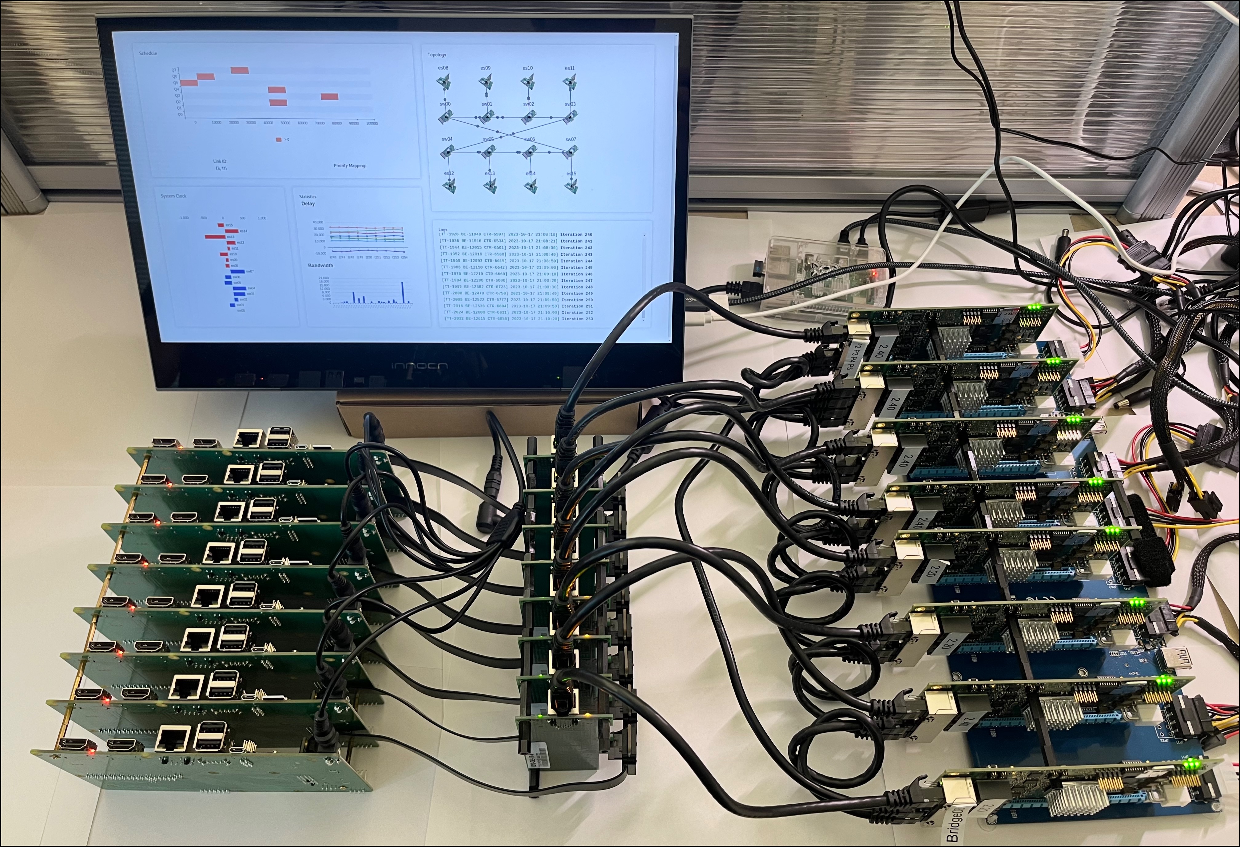
(a) Physical layout of the testbed

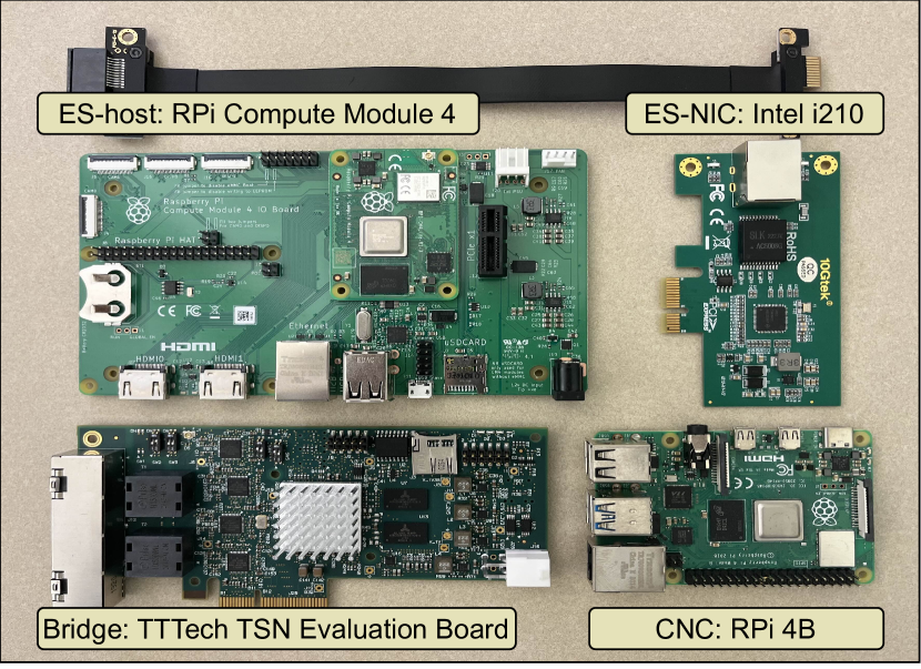
(b) Hardware components

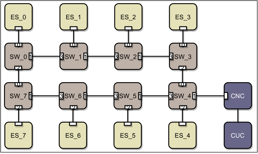
(c) Logical testbed topology

Figure 5: Overview of the TSN testbed with 8 bridges and 8 ESs

IV-A Measurements of Delays and Synchronization Error

As mentioned in Section II, most existing TAS-based scheduling methods assume that the processing delay, propagation delay, synchronization error, and clock offset on end-stations are constant or can be bounded. To the best of our knowledge, however, there is no existing study validating these assumptions through experimental measurements in real-world TSN testbeds. We argue that such validation is critical as it provides the foundation for both existing and future TAS-based scheduling method designs.

IV-A1 Propagation Delay

To measure the propagation delay, we directly connected one talker and one listener with a CAT7 cable, while measuring the round-trip time (RTT) of a stream using the hardware timestamping function supported by the NIC. As shown in Fig. 6(a), the propagation delay in this one-hop setting is bounded between 2 $ns$ and 6 $ns$, with a 4 $ns$ jitter due to the measurement variability.

IV-A2 Processing Delay

For the processing delay on the TTTech evaluation board, because we could not measure it directly, we inferred its upper bound by observing the end-to-end delay of a stream. Specifically, we gradually increased the potential upper bound of the processing delay in the TAS configuration until all frames’ end-to-end delay can be statistically bounded within the test duration. Fig. 6(b) shows that the one-hop processing delay can be bounded within 1.9 $\mu s$ in our testbed.

IV-A3 Synchronization Error

Fig. 6(c) shows the synchronization error measured on the testbed, which is reported by the logs of the Linux PTP stack. It can be observed that the synchronization error becomes stable after 5 seconds. The large values observed in the first 5 seconds are mainly due to the grand master clock election process [48]. After that, the synchronization error can be bounded within 10 $ns$.

IV-A4 Clock Offset on System

Fig. 6(d) shows the clock offset from the system clock in the application to the physical clock in the network card, which is also reported by the Linux PTP stack. Similar to the synchronization error, the clock offset is also large in the beginning, then it is bounded within 50 $ns$.

The above measurement results from our testbed confirm that the propagation delay, processing delay, and synchronization errors can all be bounded. Thus, in our subsequent simulation-based evaluation experiments, we set model assumptions of propagation delay, processing delay, synchronization error, and clock offset to be 6 $ns$, 1.9 $\mu s$, 10 $ns$, and 50 $ns$ respectively.

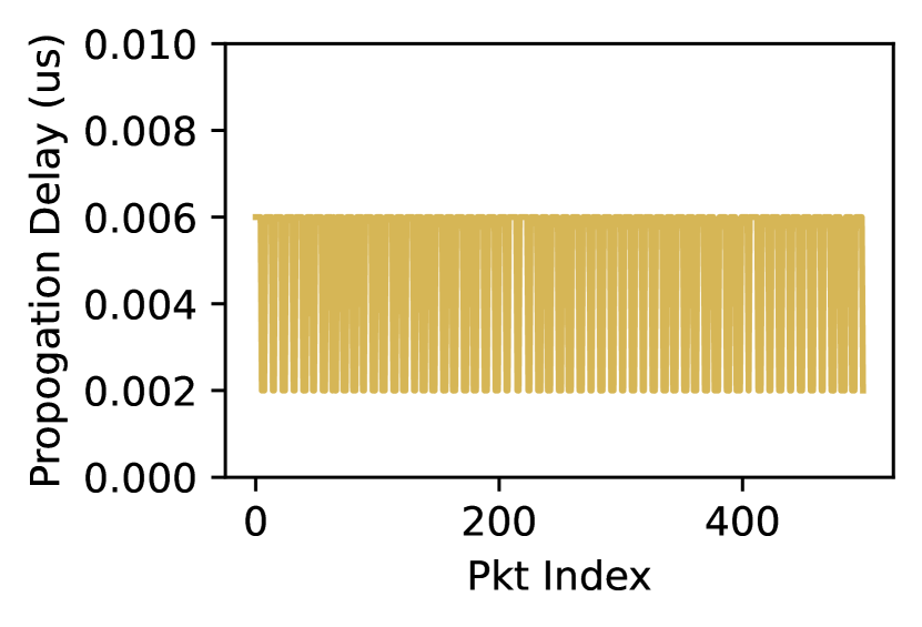
(a) Propagation delay

(b) Processing delay

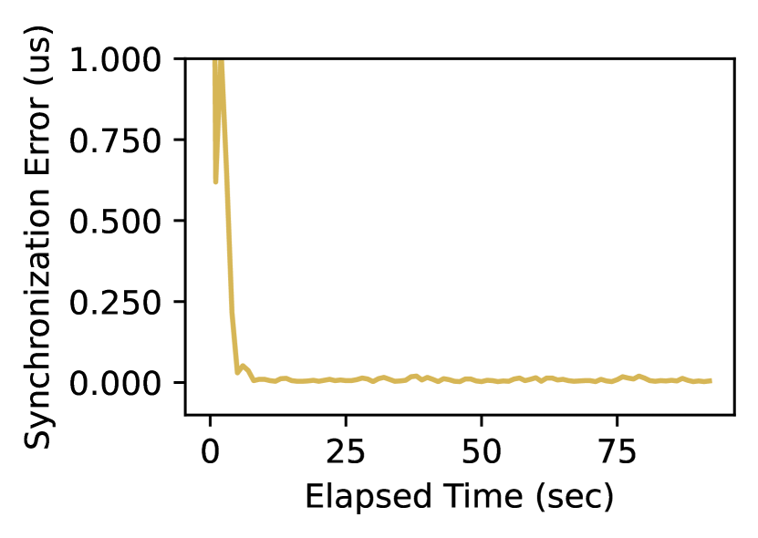
(c) Synchronization error

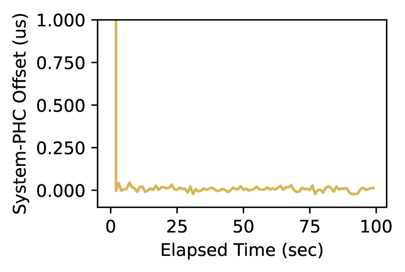
(d) Clock offset on system

Figure 6: Testbed measures on the propagation delay, processing delay, synchronization error, and system clock to physical clock offset.

IV-B Performance Validation

Before conducting extensive simulation-based experiments, we need to validate if the performance of the TSN scheduling methods is consistent on both the real-world testbed and through simulations. Such validation not only confirms the theoretical performance of each method but also ensures the correctness of our implementations. We implemented 16 out of the 17 scheduling methods on the testbed. The SMT-FRAG method was not implemented because its required fragmentation size for each stream is smaller than the window size lower bound on the hardware device.

We conducted the performance validation using a small-scale stream set consisting of 8 streams to simplify the hardware configuration. The stream set included four streams with a payload size of 100 bytes, two streams of 200 bytes, and two streams of 400 bytes. Each stream had a common period/deadline of 1 $ms$. Each stream had a unique talker but may have shared listeners. The streams were routed on the same ring topology, with their routing paths determined by the evaluated methods. After deploying the release times, queue assignments, and GCL configurations were generated from each of the 16 methods on the testbed, and we recorded the end-to-end delay of 10000 frames for each stream.

Fig. 7 and Fig. 8 compare the measured end-to-end delays of individual methods on the testbed (yellow line) and the analyzed worst-case delay from the simulation (red line). Overall, our validation results show that the real-world testbed measurements consistently remain within the bounds of the analyzed worst-case delays for all the methods.

We have two important observations from the testbed results. First, most of the streams experience a relatively stable delay ($<100ns$ variation), but some streams are observed to have delay fluctuations under certain methods. For example, Stream S0 under the JRS-MC method suffers from a gradually increasing delay during the middle of the experiment to around 1.7 $\mu s$, then it drops back to the normal state suddenly. We believe that these drifts are mainly caused by temporal loss of synchronization, widening the clock drift between the talker and the listener over time. Subsequent synchronization recovery procedures eliminate such clock drift, restoring the delay to its normal state. Secondly, a considerable gap can be observed between the testbed measurements and the analyzed delays across different methods, with a maximum gap of about 5 $\mu s$. This gap primarily stems from two factors: 1) an enforced error margin of up to 3.2 $\mu s$ by the TTTech evaluation board to accommodate timing errors on the bridge; and 2) an up to 1.9 $\mu s$ processing delay on the bridge identified during our measurements in the previous section.

V Simulation-based Experimental Setup

In this section, we present the details of our simulation-based experiment setup to evaluate the performance of the 17 scheduling methods under study.

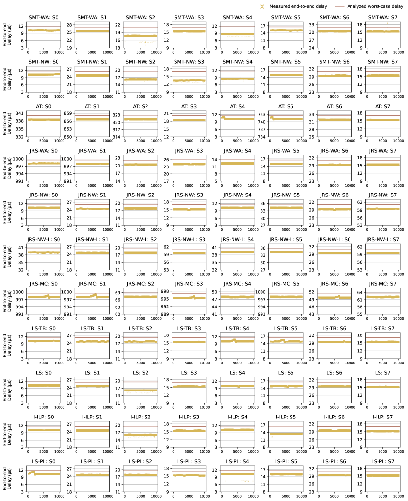
Figure 7: Performance validation on the end-to-end delays of eight TT traffic for the 16 methods on the real-world TSN testbed (Part I)

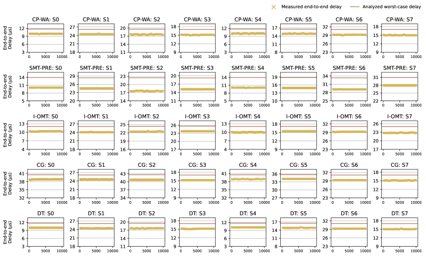
Figure 8: Performance validation on the end-to-end delays of eight TT traffic for the 16 methods on the real-world TSN testbed (Part II)

TABLE II: Parameter settings for the performance evaluation.

	Parameter	Type	Value
	Number of streams	-	{10, 40, 70, … , 190, 220}
		Sparse single	{2}
		Dense single	{0.4}
		Sparse harmonic	{0.5, 1, 2, 4}
		Dense harmonic	{0.1, 0.2, 0.4, 0.8}
		Sparse inharmonic	{0.25, 0.5, 1.25, 2.5, 4}
	Stream period ($ms$)	Dense inharmonic	{0.05, 0.1, 0.25, 0.5, 0.8}
	Number of frames	-	{8, 16, 32, … , 2048, 4096}
		Tiny size	50
		Small size	50 - 500
		Medium size	200 - 1500
		Large size	500 - 4500
	Stream payload (bytes)	Huge size	1500 - 4500
		Implicit deadline	Equal to period
		Relaxed deadline	NW + {0.1, 0.2, 0.4, 0.8, 1.6}
		Normal deadline	NW + {0.01, 0.025, 0.05, 0.1, 0.2, 0.4}
		Strict deadline	NW + {0, 0.01, 0.02, 0.025, 0.05}
Stream set	Stream deadline ($ms$)	No-wait deadline	NW
	Topology	Linear, Ring, Tree, Mesh	-
	Number of bridges	-	{8, 18, 28, … , 78}
	Number of links	-	{30, 32, 36, …, 386}
Network	Number of queues	-	8

V-A Parameter Settings

To ensure a fair evaluation among the selected TSN scheduling algorithms, we followed the parameter settings below in the experiments, which are summarized in Table II.

V-A1 Stream Set Settings

We controlled the randomly generated TSN stream set by tuning the following parameters: i) number of streams, ii) stream period, iii) number of frames, iv) stream payload, and v) stream deadline.

Number of streams. In each randomly generated stream set, the number of streams followed a uniform distribution within the range of [10, 220]. The maximum number of streams was set to 220 to encompass the settings employed in both simulation-based studies and real-world applications. Specifically, most existing studies on TSN real-time scheduling assume that the number of streams is no larger than 100 in their experiments [8]. In addition, when the number of streams reached 220, the average system utilization surpassed the recommended upper bound for industrial applications’ critical traffic recommended in  [49], resulting in a very low schedulability ratio and impractical runtime for most of the evaluated methods in our results.

Stream period. Following the TSN profile for industrial automation use cases in IEC/IEEE 60802 [31], we set the range of the stream periods as $[50\mu s,4ms]$. However, randomly generated stream periods are less meaningful as the stream periods in real-world TSN applications typically follow specific patterns in corresponding industrial sectors [50]. Thus, we defined 6 stream period types, as shown in Table II, to include all the commonly employed periodicity settings.

Number of frames. With the specified ranges for the number and periods of the streams, the number of frames from the entire stream set during a network cycle varied from 8 to 4096.

Stream payload. The stream payload size was the amount of data payload (in bytes) carried by one instance of the stream. According to the IEEE 802.1Qbv standard [5], if the payload size exceeded the MTU size (typically 1500 bytes), the stream instance could be fragmented into multiple fragments, each of which was transported by one frame. In the experiments, we defined 5 payload size types (see Table II), based on typical configurations in industrial applications.

Stream deadline. Theoretically, the minimum end-to-end (e2e) delay experienced by a stream equals to the sum of propagation delay, processing delay, and transmission delay along the routing path (i.e., the e2e delay under the no-wait model). Thus, we set the minimum deadline of each stream to its no-wait delay (denoted as NW) which can be readily calculated according to our hardware-based measurement results in Section IV. We defined 5 stream deadline types (see Table II) to aid the generation of random stream sets in our experiments.

V-A2 Network Settings

The random generation of a TSN network in our experiments was controlled by the following parameters: i) network topology, ii) number of bridges, iii) number of links, iv) number of queues, and v) line rate.

Network topology. In the experiments, we employed four commonly used topologies as shown in Fig. 9, i.e., linear topology, ring topology, tree topology, and mesh topology.

Number of bridges. We increased the number of bridges in the network to control the network size from 8 to at most 78, where the network diameter reached the synchronization accuracy limitation in IEEE 802.1AS [48] under our topologies.

Number of links. Based on the number of bridges in the network, the number of links was determined accordingly under different network topologies, as detailed in Table II.

Link rate and number of queues. In our experiments, unless specified otherwise, we employed gigabit bridges with a line rate of 1 Gbps, which is offered by most vendors [51]. The number of queues on each egress port was fixed to 8 which is a common setting in TSN bridges (e.g., TTTech Evaluation board). We also assumed that all eight queues were exclusively dedicated to handling critical TT traffic.

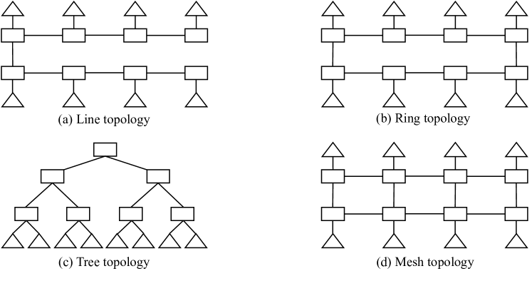
Figure 9: Four network topologies evaluated in the experiments.

V-B Algorithm Implementation

In this work, we reproduced 17 existing TAS-based scheduling methods as summarized in Table I. We implemented all the algorithms in Python3, as some works rely on third-party software which all provides an interface in Python3. Specifically, for SMT/OMT-based methods, we used the Z3 solver to support the required theories and logical formulas such as array and arithmetic theory [52]. For ILP-based methods, we used the Gurobi optimizer which is one of the most advanced ILP solvers [53].

It is worth noting that we made the following selection or modification on certain methods in our simulation studies to improve the evaluation efficiency. We use the symbol (✓) in Table I to mark the algorithms that are not implemented by us but are presented in the original paper.

SMT-WA. This work studied both the frame-based model and stream-based isolation model, showing that the frame-based approach could enhance schedulability with only a marginal runtime overhead (up to 13%). Thus, we only implemented the proposed frame-based approach in our study.

JRS-NW-L/JRS-MC. Because the model generation optimization techniques proposed in JRS-NW-L and JRS-MC were found to be counter-effective in a recent study [17], we omitted such optimizations in our simulation to reduce the execution time.

SMT-NW. The exact solution in SMT-NW was selected as it showed better overall performance in our evaluation compared with its heuristic solution.

LS-TB. We omitted the “global conflict set” data structure used in the paper as it is rarely called (only 0.96%) in the problem-solving process.

LS. The FINDIT function used in LS was not described in detail, thus we implemented it using a binary search-based strategy in our simulation.

SMT-FRAG. We only implemented the optimal method in SMT-FRAG, as the proposed fixed-priority scheduling method involved worst-case delay analysis which is difficult to implement without detailed description.

CP-WA/LS-TB. We omitted the presence variable, a decision variable was used to select streams in CP-WA and LS-TB to optimize the number of schedulable streams, as we only consider a set of streams to be schedulable when all streams can be scheduled.

I-OMT. In the OMT-based algorithms, we introduced an indicator variable to ensure that each frame is mapped to only one window. This was to simplify the time validity constraint to make the original formulation practical.

For methods that require additional parameters, we directly followed their default settings in the original papers. For example, we set the maximum number of windows to 5 for AT, the maximum fragment count to 5 for SMT-FRAG, the maximum iteration number to 100 for I-ILP, the maximum preemption count to 5 for SMT-PRE, and assume a release point at 0 for all streams in LS-TB. In addition, as suggested in the IEEE 802.1Qcc standard [34], we applied the shortest path routing algorithm to construct the routing path for each stream in FR-based methods.

V-C Evaluation Environment

Our experiments were conducted on Chameleon Cloud, an NSF-sponsored public cloud computing platform [56]. We utilized 8 nodes equipped with 2x AMD EPYC® CPUs, 64 cores per CPU with a clock speed of 2.45 GHz, and 256 GB DDR4 memory. The operating system used was Ubuntu 20.04 LTS. To make the benchmark robust and representative, we ran a total of 38400 problem instances covering all combinations of our parameter settings in Table II, with 64 experiments running simultaneously on a single node at any given time. To avoid any interference among experiments and enable concurrency, a single process with a maximum of 4 GB RAM and 4 threads was dedicated to each experiment. We set a 2-hour runtime limit for all the methods where most of them took less than 2 hours according to our evaluation. If any thread of the algorithm exceeded the time threshold, the algorithm was terminated and returned ‘unknown’. We fixed the random seeds to 1024.

V-D Evaluation Metrics

Based on the research objectives and application scenarios discussed in Section II and Section III, we summarize the commonly used evaluation metrics in Table III. As we do not consider network faults in this work, we mainly focus on the first eight metrics in our performance evaluation.

TABLE III: A Summary of the Evaluation Metrics in the study.

Evaluation	Metric	Definition
	Schedulable ratio	The ratio of schedulable stream sets
Schedulability	Schedulability advantage	The pair-wise comparison on same stream sets
	Running time	Total running time of an algorithm
Scalability	Memory usage	Peak memory usage of an algorithm
	GCL length	Maximum GCL length across all links
	Overall delay & jitter	Average end-to-end delay and jitter across all streams
	Link utilization	Maximum bandwidth utilized on links across all links
Schedule quality	Queue utilization	Maximum number of utilized queues across all links
	Reliability*	Robustness to meet traffic characters when faults occur
Fault tolerance	Integrity*	Correctness of payload information protected during faults

VI Experimental Evaluation

In this section, we perform a comprehensive simulation-based evaluation for the 17 TAS-based scheduling methods by comparing their schedulability, scalability and schedule quality using the evaluation metrics presented in Table III.

VI-A Schedulability

Given that the real-time performance is the primary focus of the studied scheduling algorithms, we first use schedulable ratio (SR) to evaluate the schedulability of all methods. Below, we first describe the evaluation setup which includes two comparison scenarios designed to minimize potential bias. We then describe the experimental results obtained from each scenario. Building upon these findings, we present both model comparisons and algorithm comparisons among the studied scheduling methods.

VI-A1 Setup

As discussed in Section V-C, we set a 2-hour timeout limit for each algorithm to prevent it from spending a long time to find a solution. In our evaluation, therefore, each method outputs one of the three results for each generated random stream set: schedulable, unschedulable, and unknown. Due to the presence of these unknown results, we are unable to precisely quantify the schedulability performance of each method. To overcome this issue, we devise two evaluation scenarios to ensure a fair performance comparison among different methods.

Evaluation Scenario 1 (ES1). In ES1, we conduct a comprehensive cross-evaluation of all 17 methods by employing a conservative statistical strategy to calculate SR. Specifically, the SR of each method is defined as the ratio of schedulable stream sets to all the generated stream sets. Such schedulable ratio plays as the schedulability lower bound because all the unknown results are deemed as unschedulable.

Although SR can to some extent reflect the schedulability of the studied scheduling methods, it can be unfair to those methods requiring higher resource consumption where a considerable portion of the stream sets with unknown results might be schedulable. To mitigate the influence of unknown results on the performance comparison, a straightforward solution is to only consider the experimental settings where all methods produce known results, i.e., schedulable or unschedulable. However, the experimental settings that will yield known results for all methods could be too small, making the performance comparison statistically insignificant.

Evaluation Scenario 2 (ES2). To tackle the above issue, in ES2, we conduct a pairwise performance comparison between any two methods by developing a novel metric, called schedulability advantage (SA), which is calculated only based on the known results for both methods. SA of A to B, denoted as $\Phi(A,B)$, quantifies the degree to which method $A$ outperforms method $B$. Specifically, $\Phi(A,B)$ represents the ratio of the number of stream sets where method $A$ returns schedulable while method $B$ returns unschedulable to the number of stream sets where both methods $A$ and $B$ return known results. Therefore, if $\Phi(A,B)>\Phi(B,A)=0$, we say that method $A$ dominates method $B$ as there does not exist any stream set where method $B$ can find a schedulable solution but method $A$ cannot.

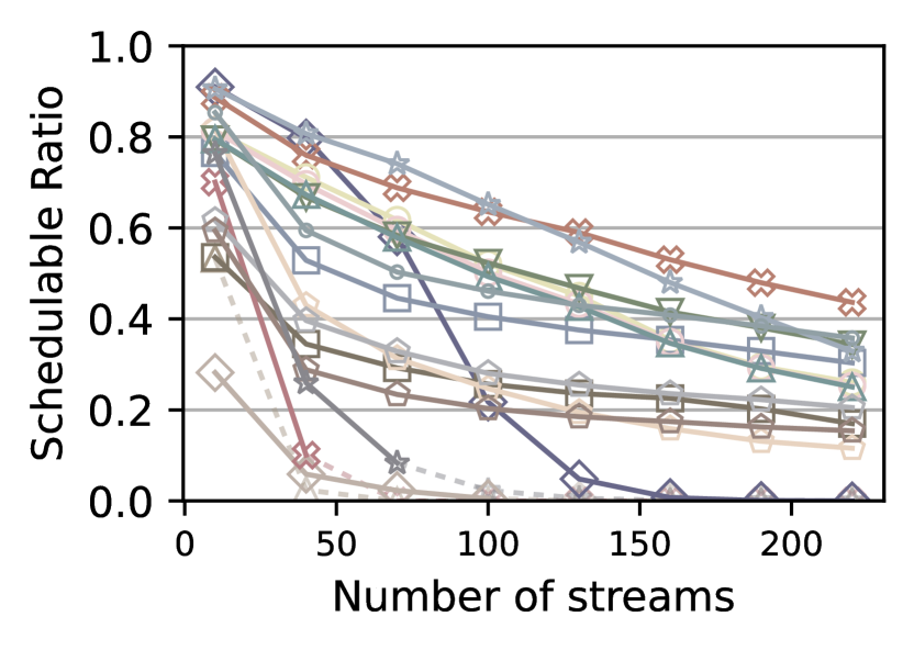
(a) Number of streams

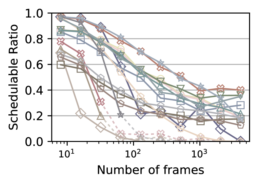
(b) Number of frames

(c) Number of bridges

(d) Number of links

Figure 10: SR comparison under different stream set and network settings by varying the parameter values.

Figure 11: Pairwise SA comparison among the studied scheduling methods.

(a) SR comparison under different periodicity pattern settings.

(b) SR comparison under different payload size settings.

(c) SR comparison under different deadline settings.

(d) SR comparison under different network topology settings.

Figure 12: SR comparison under different stream set and network settings by varying the parameter types.

VI-A2 Results

Based on the two evaluation scenarios, we conduct extensive experiments under various stream set settings and network settings as described in Section V-A.

In the first set of experiments, we evaluate the SRs of all the methods by varying the parameter settings summarized in Table II. Specifically, Fig. 10 shows the SR as functions of the number of streams, number of frames, number of bridges, and number of links, respectively. In each subfigure, only one parameter is varied with all other parameters being fixed. We use dashed lines to denote data points comprising over 90% unknown results. Fig. 12 shows the SR of each method under different stream period types, stream payload types, stream deadline types, and topologies, respectively.

In the second set of experiments, we perform the pairwise comparison using the SA metric and the results are shown in a heatmap in Fig. 11. Specifically, each cell represents the $\Phi({A},{B})$ value, where the row-index represents method ${A}$ and the column-index represents method ${B}$. Darker cells signify higher SA values, while light yellow represents a zero SA value. Moreover, on the vertical axis, methods are sorted from high to low based on their average SA values.

VI-A3 Discussion

Based on the obtained experimental results, we now present our discussion across two dimensions of granularity. First, we perform evaluation comparisons among different scheduling models discussed in Section II-C to show their pros and cons. Next, we delve into the performance evaluation of individual scheduling algorithms to discuss their advantages and limitations.

Model comparisons. We discuss the model comparison results by categorizing two sets of different scheduling models: a) models with varied performance, and b) models with stable performance between SR and SA. This classification is based on their observed trends in our experiments. The first set of comparisons includes: 1) joint routing/scheduling (JRS) model and fixed routing (FR) model, 2) fragmentation/preemption-allowed (FRAG/PRE) model and non-fragmentation/preemption (non-FRAG/non-PRE) model, and 3) no-wait model and wait-allowed model. The second set of comparisons includes: 1) fully and partially schedulable models, 2) frame-based model and window-based model.

a) Models with varied performance. We find that although a complex model can achieve higher SA, it also incurs higher computation overhead, which may significantly limits its performance on SR. Our experimental results confirm this observation consistently across the following three sets of comparisons:

•  JRS vs. FR model. We find that JRS model dominate FR model under either wait-allowed or no-wait model in terms of SA in Fig. 11. For example, JRS-WA and JRS-NW-L dominate their counterparts under the FR model (SMT-WA and CP-WA) and JRS-NW dominate its counterpart SMT-NW. However, the JRS model usually leads to lower SR compared to the FR model due to their incurred computation overhead. As shown in Fig. 10, along with the increase of the network scale (Fig. 10(c)-(d)), the methods under the JRS model suffer larger performance degradation by 24.9% on average compared to that of the methods under FR model by 11.9% on average. A similar trend can also be observed in Fig. 12(d). By changing the network topology from line/tree to ring/mesh, the SR of JRS-WA degrades by 28.7% on average. A similar pattern can also be observed from other methods under the JRS model such as JRS-MC and I-ILP.

•  FRAG/PRE vs. non-FRAG/non-PRE model. In Fig. 11, SMT-FRAG and SMT-PRE show the average SA values of 14.7% and 14.0%, respectively, outperforming the average of other methods at 10.4%. However, these methods experience significantly reduced schedulability due to their larger computational overhead. For example, in Fig. 10(a)(b), although SMT-FRAG and SMT-PRE start with very high SR (70.1% and 76.4% respectively), their SR degrades sharply to below 10.0% after the number of streams and frames are increased to 70 and 128, respectively. This poor SR performance can be consistently observed by varying other parameters in Fig.10(c)(d) and Fig.12.

•  No-wait vs. wait-allowed model. The initial comparison between two FR-based methods (SMT-NW and SMT-WA), suggests that the wait-allowed method dominates the no-wait method on SA as expected due to its more flexible delay model from Fig. 11. However, on the SR performance, SWT-NW surpasses SWT-WA when the workload is increased to 70 streams or 64 frames in Fig. 10(a)(b), and SWT-NW consistently outperforms SWT-WA in Fig. 10(c)(d). A similar pattern can be observed under JRS methods (e.g., JRS-NW and JRS-WA) that JRS-WA dominates JRS-NW on SA, but their difference in SR is negligible.

b) Models with stable performance. We also find that in some methods, the schedulability improvement from models outweighs its increased computational overhead, which leads to consistent performance improvement on both SA and SR. Our experimental results validate this statement across the following two set of comparisons:

•  Fully vs. partially schedulable model. We compare LS with LS-PL and LS-TB methods, all rooted in the LS-based heuristic approach. As shown in Fig. 11, the fully schedulable model LS shows higher SA (7.24%) than the partially schedulable model LS-PL (2.8%) and LS-TB (4.29%). The comparison results are retained when evaluating the SR performance. As shown in Fig. 10, the fully schedulable model LS also consistently outperforms the partially schedulable model LS-TB and LS-TL under varied workload and network scale parameters. Combined with the comparison results of no-wait/wait-allowed model, these results may imply that enlarging the search space on the end-station side (fully schedulable/partially schedulable) is more effective than enlarging the search space on the bridge side (no-wait/wait-allowed).

•  Frame-based vs. window-based model. We compare AT with SMT-NW and SMT-WA which are all SMT-based exact approaches. As shown in Fig. 11, the frame-based methods SMT-NW and SMT-WA dominate the window-based method AT on SA. Consistently, as shown in Fig. 10, both SMT-NW and SMT-WA also consistently outperform AT in terms of SR by increasing either the workload or network scale. These results imply that the constraints applied on GCL length may significantly limit the schedulability.

Based on the above results and discussions on different scheduling models, we conclude with the following finding.

Finding 1. Although complex scheduling models can enhance the schedulability in theory, their incurred high computational overhead reduces the performance improvement in practice. They may even have counterproductive effects in resource-constrained systems.

Algorithm comparisons. We now present the performance comparison in terms of schedulability among individual scheduling methods. According to the classification of scheduling methods in Table I, each method is either a heuristic or exact solution. Thus, we first perform comparisons between heuristic approaches and exact solutions. We then delve into heuristic approaches to examine the properties derived by individual heuristic designs.

a) Heuristic vs. exact solutions. Apparently, although heuristic approaches may not match the performance of exact solutions, they show higher efficiency, especially under heavy workloads and restricted computational resources. Our experimental results align with this expectation. For example, comparing the SR of FR-based wait-allowed methods in Fig. 10(a), the exact solution SMT-WA outperforms heuristic LS-TB when the number of streams is less than 100. However, when the number of streams keeps increasing, LS-TB remains relatively stable, but SMT-WA rapidly declines to zero. Similar trends can also be found in Fig. 12 for the same method.

Due to their inherent efficiency, heuristic approaches can also benefit more from complex models compared to exact solutions. For example, comparing SR for the no-wait scheduling methods in Fig. 10(a), heuristic CG and exact solution JRS-NW exhibit similar SR when the number of streams is less than 80. However, when the stream set size increases, CG outperforms JRS-NW with a widening gap. Similar trends can also be found in many other pairwise methods under the same scheduling models, e.g., AT and I-OMT.

b) Comparison among heuristic algorithms. Our experiment results show that the performance of four heuristic algorithms significantly degrades under certain specific scenarios. 1) For networks with routable topologies (i.e., ring and mesh), I-ILP demonstrates lower schedulability due to the inefficiency of its DAMR routing algorithm. For example, as shown in Fig. 12(d), SRs of I-ILP drop from 41.6% under line topology and 54.6% under tree topology to 9.6% under ring topology and 7.4% under mesh topology. 2) LS-PL suffers from a notably low SR (7.0%) in networks with ring topology as shown in Fig. 12(d). This is mainly due to the high likelihood of cyclic dependencies, causing frequent failures in its phase division algorithm. 3) Under strict deadline settings, both LS-TB and LS-PL show low schedulability due to their partially schedulable traffic model. This deficiency results in a drop in SR from implicit deadline setting (51.9%) to no-wait deadline setting (1.0%) as shown in Fig. 12(c). 4) In the presence of inharmonic periodicity, I-OMT exhibits a reduced SR (10.4%), a consequence of its restricted number of GCL entries compared to the single sparse method (66.4%) as shwon in as shown in Fig. 12(a). This decrease is primarily due to scheduling conflicts, where a high volume of frames rapidly exhausts the limited GCL entries.

Finding 2. Schedulability optimization is highly context-dependent. There is no universally superior scheduling algorithm (neither an exact nor specific heuristic algorithm); instead, the best approach depends on the specific requirements and constraints of the scenario.

VI-B Scalability

In this section, we compare the scalability of 17 scheduling methods in terms of runtime and memory consumption under different settings. Runtime and memory consumption are both critical performance metrics that evaluate how well the scheduling algorithm will scale in practice [57].

VI-B1 Setup

In our experiments, the runtime of a scheduling algorithm consists of the pre-processing time (filtering the invalid solution space), the constraint adding time, and the problem solving time. If a scheduling method follows an objective function, we only measure its runtime of determining a feasible solution, rather than the optimal one to avoid any unfair comparison. For the memory consumption, we track the maximum memory usage for each approach, setting a 4GB threshold to allocate enough RAM and avoid swap space use.

(a) Number of streams

(b) Number of streams

(c) Number of bridges

(d) Number of bridges

Figure 13: Runtime and memory consumption comparisons under varied stream set and network settings.

(a) Runtime correlation

(b) Memory correlation

Figure 14: Runtime and memory consumption correlation in diverse scenarios.

VI-B2 Results

Fig. 13 displays how runtime and memory consumption vary with the increase in the number of streams and bridges. Fig. 14 presents two separate analyses focusing on the correlation between algorithm runtime and various settings, as well as the correlation between memory consumption and various settings, respectively. The Pearson correlation coefficient is utilized to quantify the correlation in both analyses, indicating a positive correlation through red color and a negative correlation through blue color. A high absolute correlation for a method signifies its sensitivity to that particular factor, implying that targeted scalability enhancements can be explored for that factor.

VI-B3 Discussion

Based on the above experimental results, we have two key findings on how experimental settings and algorithm design affect the runtime and memory usage.

Overall trend. From Fig. 13(a)-(b), as the number of streams increases, we observe a significant rise in both the runtime and memory consumption for most methods. Specifically, the average runtime of all methods increases from 9.3 minutes under 10 streams to 48.6 minutes under 220 streams. Likewise, the average memory consumption increases from 476 MB under 10 streams to 1800 MB under 220 streams. Interestingly, adding more bridges to the network has a limited effect on the runtime. Overall, as shown in Fig. 13(c), the runtime of most methods slightly increases from 23.6 minutes with 8 bridges to 34.1 minutes with 88 bridges. Among them, FR-based methods only show a modest increase from 25.4 to 29.2 minutes, but JRS-based methods show a more substantial rise from 19.2 minutes to 41.8 minutes.

Regarding the memory consumption as shown in Fig. 13(d), it remains relatively steady for FR-based methods with a slightly average increase of 183 MB when the number of bridges is increased from 8 to 88. As an exception, JRS-based methods peak at an average of 2070 MB with 48 bridges before dropping. These complex trends of memory and runtime along with the increased network scale may be due to compound factors. For example, a larger network can extend routing paths, thereby requiring more scheduling effort, but simultaneously reducing traffic density to lower the chance of collisions. These observations suggest that a larger network size does not necessarily result in a proportionally increased problem size, such as an increase in the number of decision variables or constraints.

Finding 3. The increased workload poses a significant challenge to TSN scheduling, whereas the increased network scale has little impact on the scalability under our experimental settings.

Individual algorithms. We also explore potential scalability patterns and bottlenecks for individual methods by analyzing their runtime and memory consumption correlation. As shown in Fig. 14, a common trend observed in all methods is a positive correlation between runtime and memory consumption with the number of flows, frames, and utilization. However, distinct patterns can also be observed for individual methods. For instance, the runtime of I-OMT exhibits higher sensitivity to changes in the number of flows (correlation coefficient of 0.48) than its memory consumption (correlation coefficient of 0.10). In contrast, SMT-FRAG demonstrates a more significant increase in memory consumption when the number of flows is increased (correlation coefficient of 0.90) compared to its runtime (correlation coefficient of 0.24).

Finding 4.: Different scheduling methods exhibit diverse runtime and memory consumption patterns under different settings. A general solution might not exist to handle the diverse factors that can enhance the scalability of all methods.

VI-C Schedule Quality

The schedulability and scalability metrics demonstrate the effectiveness and efficiency of each scheduling method in finding a feasible solution. In addition, we are also interested in the quality of the solution (i.e., the generated schedule). In this section, we evaluate the solution quality of 17 methods in terms of GCL length, end-to-end delay and jitter, link utilization, and queue utilization.

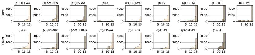
Figure 15: Rank distribution of the maximum GCL length among all the problem instances.

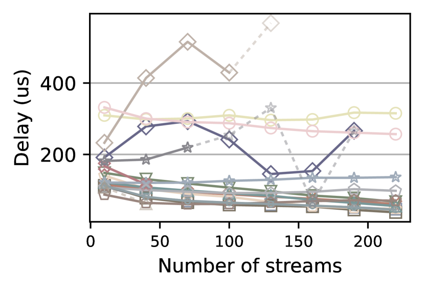
(a) Delay vs. # of streams

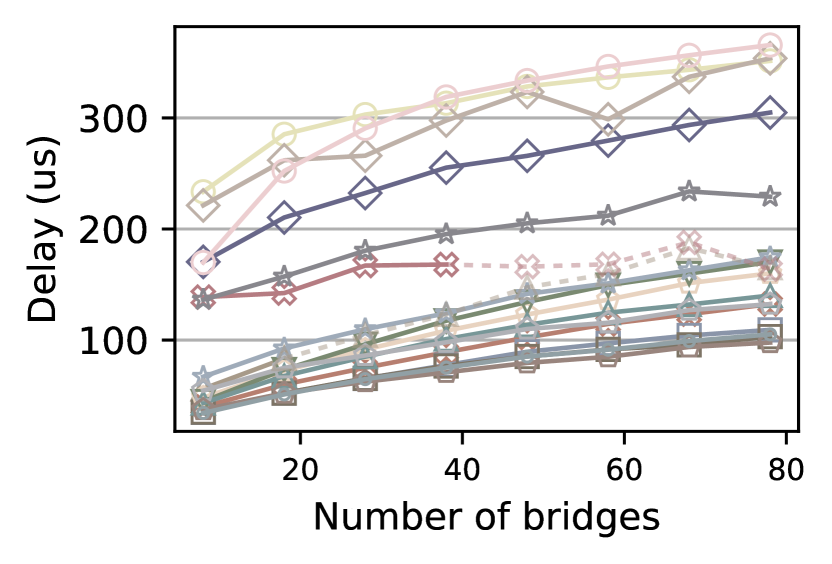
(b) Delay vs. # of bridges

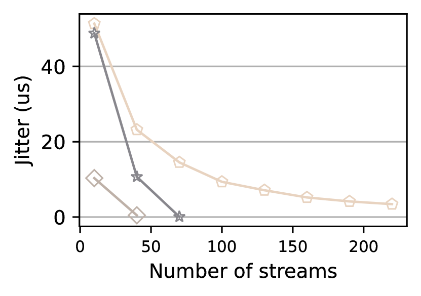
(c) Jitter vs. # of streams

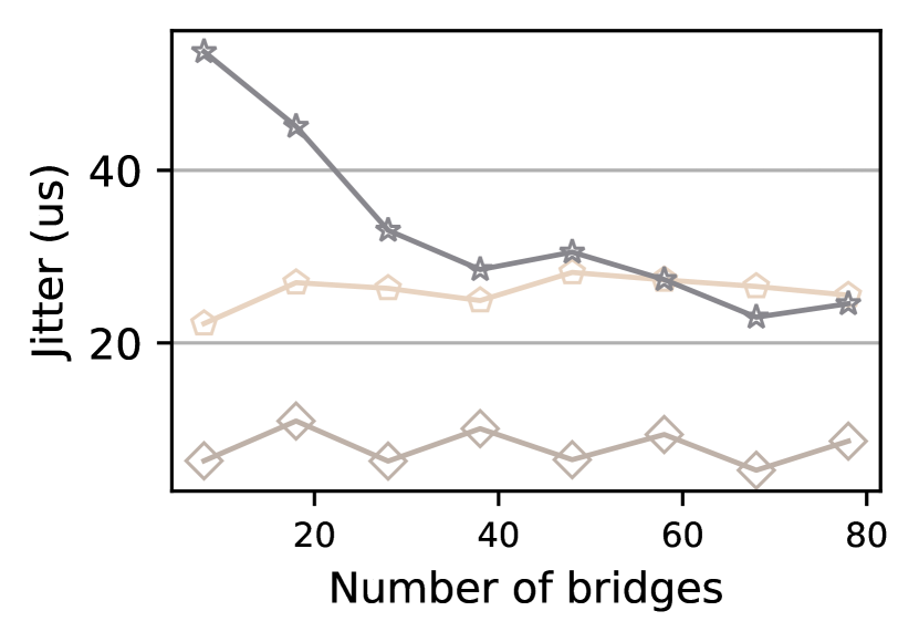
(d) Jitter vs. # of bridges

Figure 16: Delay and jitter vs. # of streams and bridges

Figure 17: Rank distribution of the maximum link utilization among all the solvable problem instances for each method.

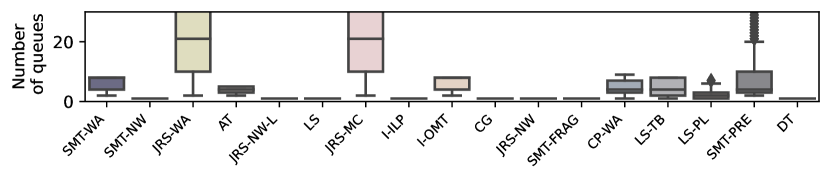
Figure 18: Distribution of the maximum queue utilization among all solvable problem instances for each method.

VI-C1 Setup

In our experiment, we define the GCL length as the peak value, i.e., the number of GCL entries for the port with the maximum value across the entire network. The average end-to-end delay is calculated for all streams, denoted from the moment when its first bit leaves the talker until the last bit is received at the listener. Similarly, we define the jitter as the difference between the maximum and minimum delays for each frame in individual streams, then average these values across all streams. Moreover, the link utilization is computed as the highest observed ratio between the allocated window size and the network cycle across all links. Lastly, we analyze the queue utilization, identifying the maximum required queues across all links.

Because individual methods can yield different feasible solutions due to their inherent schedulability characteristics, it is challenging to compare the schedule quality without any bias. In our evaluation results, we find that the GCL length and link utilization are highly sensitive to the schedulability of the method. To tackle this problem, we define a rank-based metric that aims to generate a more representative comparison utilizing all feasible solutions. The key idea is to leverage the obtained performance of each method and the generality of each problem instance to reduce the bias. Let $\mathbb{M}$ be the set of all methods, and for any given problem instance, $\mathbb{S}$ be the subset of methods that produce feasible results. The rank, $R({M})$, for a method ${M}\in\mathbb{S}$ is defined as $R({M})=(|\mathbb{M}|-|\mathbb{S}|)+r({M})$, where $r({M})$ is the relative rank of method ${M}$ within $\mathbb{S}$ based on its performance, $|\mathbb{M}|-|\mathbb{S}|$ is the number of methods that fail to produce a feasible result. Methods with identical performance will receive the same rank. The lower rank value indicates better performance.

VI-C2 Results

Fig. 15 illustrates the rank distribution of the maximum GCL length for each method. The x-axis represents $R(M)$, and the y-axis denotes the frequency of each rank occurring in their feasible results. Fig. 16 shows the average end-to-end delay and jitter values across each method, which vary based on the stream set and network size. Fig. 17 displays the rank distribution of the peak link utilization of each method. Lastly, Fig. 18 presents the distribution of the maximum queue utilization across all solvable instances for each method.

VI-C3 Discussion

Based on these results, we now discuss the schedule quality of each method.

GCL length. First of all, we find that methods based on the window-based model require fewer GCL entries, resulting in shorter GCL lengths. For instance, as shown in Fig. 15, the window-based method AT mostly produces solutions with a low rank ($\leq$ 5), reflecting its strict constraint on the maximum number of windows per link. Another window-based method I-OMT aims to minimize the number of GCL entries, and also shows a relatively low rank compared with others. Secondly, we also observe that the JRS-based methods tend to have a lower rank, especially compared to FRS-based methods, which rarely have instances with a rank of $\leq 8$. This is because the routing decisions help balance the workload across the network, avoiding having high volume traffic on a single link, which could lead to a large number of windows. In addition, beyond rank distribution, our raw data shows that many frame-based methods, without optimizing GCL length, result in over 2000 entries in some instances. This exceeds the usual maximum GCL length allowed for TSN bridges, which is between 8 and 1024 [15].

End-to-end delay and jitter. For the overall trend, Fig. 16(b) shows that the growing network scale significantly increases the end-to-end delay from an average value of 92 $\mu s$ to 192 $\mu s$ when the number of bridges is increased from 10 to 80, but the stream set scale, as shown in Fig. 16(a), has limited impact. Additionally, our results also confirm that the no-wait model can significantly reduce the delay as expected compared with the window-based model, whereas the JRS model incurs a higher delay than the FR model as expected. For the jitter, interestingly, Fig. 16(c)(d) shows a decreasing jitter when more streams or bridges are added to the network. We believe this is due to the fact that a larger workload and network scale require tighter window size to ensure schedulability, which leads to a more deterministic schedule.

Link utilization. We find that the JRS model outperforms the FR model in managing link utilization. In Fig. 17, JRS-based methods (e.g., JRS-NW, JRS-WA, JRS-MC and CG) exhibit lower link utilization compared to FR methods due to their inherent load-balancing capacity. In addition, the window-based method I-OMT tends to overcommit resources, as it frequently performs the highest rank in link utilization compared to other methods.

Queue utilization. Fig. 18 shows that methods like JRS-WA, JRS-MC, and SMT-PRE, which are based on the unrestricted queuing model, often require a large number of allocated queues to ensure schedule correctness. This often surpasses the maximum number of available queues in our experimental settings. On the other hand, the explicit queuing model and no-wait model have lower queue utilization because of their explicit queuing constraints.

Finding 5. Selecting an appropriate scheduling method is crucial for achieving the desired schedule quality, as performance varies across methods.

VII Takeaway lessons

In this section, we summarize the takeaway lessons from this study, aiming to provide guidance on fair performance evaluation and future research directions in TSN real-time scheduling algorithm design.

VII-A Fair Performance Evaluation

Through our extensive studies on the 17 TSN scheduling methods, we find that the experimental setting has a significant impact on the evaluation results. As a result, research studies may make unfair comparisons under specific experimental settings and result in biased conclusions. We share the following takeaway lessons according to our experimental studies.

Parameter settings. For the sake of fair comparison, we propose two possible ways to avoid bias. 1) Deploy extensive experimental settings to include a broader range of stream set and network settings, and resource constraints. In this way, we can better understand the overall performance of a method and thus improve the fidelity and applicability of the evaluation. 2) If the computational resources are limited for performing extensive experiments, an alternative way is to select representative experiment settings based on real-world industrial scenarios or from standards and profiles. For instance, [31, 49] offer realistic use cases that can serve as common evaluation scenarios. However, given the early stage of TSN-based research, the availability of real-world industrial scenarios and standardized profiles is still limited.

Experiment description. Another takeaway lesson is to provide detailed description of the experimental settings used in the evaluation. The absence of such information may lead to inconsistent results for researchers who would like to replicate the method. Below we summarize some experimental settings that have a significant impact on the evaluation results and need to be explained in detail. 1) Model assumption. Instead of simply stating that “we compare with [14]”, it is better to clarify that “we adapt [14] to a partially schedulable model that incorporates frame-isolation constraints. The Z3 solver is utilized with default configuration and without objective function.” 2) Stream set and network specification. It is crucial to present the detailed specifications, e.g., the stream period (deadline) range, stream payload, and how the problem instances are sampled from specifications. 3) Evaluation metrics. It is important to specify how the evaluation metrics are measured. For example, is the delay measured starting from the time when the frame leaves the end station or the time when it arrives at the first bridge? And, is the jitter calculated as the standard variance in delay across all frames or the maximum difference in delay between any two frames?

VII-B Algorithm Design

In addition to the experiment designs, we also provide below some insights and recommendations to guide future research on TAS-based real-time scheduling design.

Real-world constraints. In our testbed validation, we identifiy several issues that prevent existing scheduling methods from ensuring end-to-end delay on a real-world testbed due to ignoring some practice constraints. These findings offer insights for future TSN research. 1) Co-scheduling of data streams and synchronization messages. We find that collisions between TT traffic and PTP messages can occur and cause synchronization losses, resulting in network failure or deadline miss of TT traffic. This is because, in TSN scheduling, a maximum sync error is included in the modeling. However if synchronization cannot be performed in the pre-defined period due to interference from other TT traffic, a sync error will become larger than the maximum error defined in the modeling. 2) End stations may impose stricter constraints than TSN bridges due to their limited network processing capability and the presence of other applications. For instance, we have to insert a large inter-frame distance between TT frames to maintain the packet order on the end stations. This requirement is overlooked by most of the existing methods. 3) TSN bridge may be subject to a specific window size bound in GCL; however, only a few methods include this constraint by adding a granularity variable to their models. If these factors are overlooked during the schedule generation, adapting the schedule to the testbed will become challenging if not impossible. Hence, we suggest including these real-world constraints in future studies to improve the practicality of the proposed scheduling methods.

Performance optimization for specific scenarios. As we point out in the findings described in Section VI, it is important to select the right model and scheduling method for performance optimization under specific scenarios. Below, we summarize the pros and cons of certain models and methods observed from our experiments. First of all, simple models (e.g., no-wait model) or heuristic approaches (e.g., the list scheduler) can achieve better performance for stream sets with large workload. Second, methods based on the JRS model can be counter-effective in large-scale network settings compared with the FR model due to its low efficiency. Third, methods based on the window-based model tend to optimize the GCL length, whereas JRS-based methods usually lead to lower link utilization. Finally, the no-wait model is preferred if the number of queues is restricted.

Automatic and intelligent model/method selection. Given all the challenges of performance optimization in TSN scheduling as discussed above, it would be helpful to develop an easy-to-use toolkit that is able to perform intelligent model/method selection and automatic schedule generation. Such a tool can significantly reduce the complexity of the scheduling method design for TSN networks.

VIII Conclusion and Future Work

The growing R&D interests in time-sensitive networking (TSN) aim to achieve ultra-low latency and deterministic communications over switched Ethernet networks. This paper examines 17 state-of-the-art real-time scheduling methods based on Time-aware Shaper (TAS) and establishes a benchmark for performance evaluation using various performance metrics. Comprehensive experiments are conducted using both high-fidelity simulator and real-world testbed to compare these algorithms, highlighting their strengths and weaknesses under various scenarios. This paper aims to assist researchers in identifying the current state and open problems in TSN scheduling algorithm design and implementation, offering insights towards future TSN research and development.

For the future work, we will enhance the experimental study by incorporating realistic problem instances from avionic and automobile industries, as well as incorporating the fault tolerance scenarios into the evaluation. To further evaluate the correctness and practicability of the existing TAS scheduling methods, we will conduct more comprehensive empirical experiments on our TSN testbed. Finally, we will encourage the community to utilize our open-source dataset and source code to evaluate their scheduling methods to boost the development of TSN-related R&D projects.

IX Acknowledgement

The work is supported in part by the National Science Foundation Grant CNS-1932480, CNS-2008463, CCF-2028875, CNS-1925706, and the NASA STRI Resilient Extraterrestrial Habitats Institute (RETHi) under grant number 80NSSC19K1076.

References

- [1] E. Sisinni, A. Saifullah, S. Han, U. Jennehag, and M. Gidlund, “Industrial internet of things: Challenges, opportunities, and directions,” IEEE transactions on industrial informatics, vol. 14, no. 11, pp. 4724–4734, 2018.
- [2] W. Z. Khan, M. Rehman, H. M. Zangoti, M. K. Afzal, N. Armi, and K. Salah, “Industrial internet of things: Recent advances, enabling technologies and open challenges,” Computers & Electrical Engineering, vol. 81, p. 106522, 2020.
- [3] “Ieee standard for local and metropolitan area networks– virtual bridged local area networks amendment 12: Forwarding and queuing enhancements for time-sensitive streams,” IEEE Std 802.1Qav-2009, pp. 1–72, 2010.
- [4] “Ieee standard for local and metropolitan area networks–bridges and bridged networks - amendment 34:asynchronous traffic shaping,” IEEE Std 802.1Qcr-2020, pp. 1–151, 2020.
- [5] “Ieee standard for local and metropolitan area networks – bridges and bridged networks - amendment 25: Enhancements for scheduled traffic,” IEEE Std 802.1Qbv-2015, pp. 1–57, 2016.
- [6] L. Zhao, P. Pop, and S. Steinhorst, “Quantitative performance comparison of various traffic shapers in time-sensitive networking,” IEEE Transactions on Network and Service Management, vol. 19, no. 3, pp. 2899–2928, 2022.
- [7] D. Hellmanns, J. Falk, A. Glavackij, R. Hummen, S. Kehrer, and F. Dürr, “On the performance of stream-based, class-based time-aware shaping and frame preemption in tsn,” in 2020 IEEE International Conference on Industrial Technology (ICIT). IEEE, 2020, pp. 298–303.
- [8] T. Stüber, L. Osswald, S. Lindner, and M. Menth, “A survey of scheduling in time-sensitive networking (tsn),” arXiv preprint arXiv:2211.10954, 2022.
- [9] A. Minaeva and Z. Hanzálek, “Survey on periodic scheduling for time-triggered hard real-time systems,” ACM Computing Surveys (CSUR), vol. 54, no. 1, pp. 1–32, 2021.
- [10] L. Deng, G. Xie, H. Liu, Y. Han, R. Li, and K. Li, “A survey of real-time ethernet modeling and design methodologies: From avb to tsn,” ACM Computing Surveys (CSUR), vol. 55, no. 2, pp. 1–36, 2022.
- [11] A. Nasrallah, A. S. Thyagaturu, Z. Alharbi, C. Wang, X. Shao, M. Reisslein, and H. ElBakoury, “Ultra-low latency (ull) networks: The ieee tsn and ietf detnet standards and related 5g ull research,” IEEE Communications Surveys & Tutorials, vol. 21, no. 1, pp. 88–145, 2018.
- [12] Y. Seol, D. Hyeon, J. Min, M. Kim, and J. Paek, “Timely survey of time-sensitive networking: Past and future directions,” IEEE Access, vol. 9, pp. 142 506–142 527, 2021.
- [13] A. Nasrallah, V. Balasubramanian, A. Thyagaturu, M. Reisslein, and H. ElBakoury, “Tsn algorithms for large scale networks: A survey and conceptual comparison,” arXiv preprint arXiv:1905.08478, 2019.
- [14] S. S. Craciunas, R. S. Oliver, M. Chmelík, and W. Steiner, “Scheduling real-time communication in ieee 802.1 qbv time sensitive networks,” in Proceedings of the 24th International Conference on Real-Time Networks and Systems, 2016, pp. 183–192.
- [15] R. S. Oliver, S. S. Craciunas, and W. Steiner, “Ieee 802.1 qbv gate control list synthesis using array theory encoding,” in 2018 IEEE Real-Time and Embedded Technology and Applications Symposium (RTAS). IEEE, 2018, pp. 13–24.
- [16] E. Schweissguth, P. Danielis, D. Timmermann, H. Parzyjegla, and G. Mühl, “Ilp-based joint routing and scheduling for time-triggered networks,” in Proceedings of the 25th International Conference on Real-Time Networks and Systems, 2017, pp. 8–17.
- [17] D. Hellmanns, L. Haug, M. Hildebrand, F. Dürr, S. Kehrer, and R. Hummen, “How to optimize joint routing and scheduling models for tsn using integer linear programming,” in 29th International Conference on Real-Time Networks and Systems, 2021, pp. 100–111.
- [18] J. Falk, F. Dürr, and K. Rothermel, “Exploring practical limitations of joint routing and scheduling for tsn with ilp,” in 2018 IEEE 24th International Conference on Embedded and Real-Time Computing Systems and Applications (RTCSA). IEEE, 2018, pp. 136–146.
- [19] E. Schweissguth, D. Timmermann, H. Parzyjegla, P. Danielis, and G. Mühl, “Ilp-based routing and scheduling of multicast realtime traffic in time-sensitive networks,” in 2020 IEEE 26th International Conference on Embedded and Real-Time Computing Systems and Applications (RTCSA). IEEE, 2020, pp. 1–11.
- [20] F. Dürr and N. G. Nayak, “No-wait packet scheduling for ieee time-sensitive networks (tsn),” in Proceedings of the 24th International Conference on Real-Time Networks and Systems, 2016, pp. 203–212.
- [21] M. Vlk, K. Brejchová, Z. Hanzálek, and S. Tang, “Large-scale periodic scheduling in time-sensitive networks,” Computers & Operations Research, vol. 137, p. 105512, 2022.
- [22] M. Pahlevan, N. Tabassam, and R. Obermaisser, “Heuristic list scheduler for time triggered traffic in time sensitive networks,” ACM Sigbed Review, vol. 16, no. 1, pp. 15–20, 2019.
- [23] X. Jin, C. Xia, N. Guan, and P. Zeng, “Joint algorithm of message fragmentation and no-wait scheduling for time-sensitive networks,” IEEE/CAA Journal of Automatica Sinica, vol. 8, no. 2, pp. 478–490, 2021.
- [24] A. A. Atallah, G. B. Hamad, and O. A. Mohamed, “Routing and scheduling of time-triggered traffic in time-sensitive networks,” IEEE Transactions on Industrial Informatics, vol. 16, no. 7, pp. 4525–4534, 2019.
- [25] M. Vlk, Z. Hanzálek, and S. Tang, “Constraint programming approaches to joint routing and scheduling in time-sensitive networks,” Computers & Industrial Engineering, vol. 157, p. 107317, 2021.
- [26] X. Jin, C. Xia, N. Guan, C. Xu, D. Li, Y. Yin, and P. Zeng, “Real-time scheduling of massive data in time sensitive networks with a limited number of schedule entries,” IEEE Access, vol. 8, pp. 6751–6767, 2020.
- [27] Y. Zhou, S. Samii, P. Eles, and Z. Peng, “Time-triggered scheduling for time-sensitive networking with preemption,” in 2022 27th Asia and South Pacific Design Automation Conference (ASP-DAC). IEEE, 2022, pp. 262–267.
- [28] J. Falk, F. Dürr, and K. Rothermel, “Time-triggered traffic planning for data networks with conflict graphs,” in 2020 IEEE Real-Time and Embedded Technology and Applications Symposium (RTAS). IEEE, 2020, pp. 124–136.
- [29] D. Bujosa, M. Ashjaei, A. V. Papadopoulos, T. Nolte, and J. Proenza, “Hermes: Heuristic multi-queue scheduler for tsn time-triggered traffic with zero reception jitter capabilities,” in Proceedings of the 30th International Conference on Real-Time Networks and Systems, 2022, pp. 70–80.
- [30] I. S. Association et al., “Ieee standard for local and metropolitan area network–bridges and bridged networks,” IEEE Std 802.1 Q-2018 (Revision of IEEE Std 802.1 Q-2014), pp. 1–1993, 2018.
- [31] J. Dorr, K. Weber, and S. Zuponcic, Use Cases IEC/IEEE 60802. [Online]. Available: https://www.ieee802.org/1/files/public/docs2018/60802-industrial-use-cases-0918-v13.pdf
- [32] L. Zhao, P. Pop, Z. Zheng, and Q. Li, “Timing analysis of avb traffic in tsn networks using network calculus,” in IEEE Real-Time and Embedded Technology and Applications Symposium (RTAS), 2018, pp. 25–36.
- [33] S. S. Craciunas, R. S. Oliver, and T. Ag, “An overview of scheduling mechanisms for time-sensitive networks,” Proceedings of the Real-time summer school LÉcole dÉté Temps Réel (ETR), pp. 1551–3203, 2017.
- [34] “Ieee standard for local and metropolitan area networks-bridges and bridged networks-amendment 31: stream reservation protocol (srp) enhancements and performance improvements,” IEEE Std 802.1 Qcc-2018, 2018.
- [35] A. Mascis and D. Pacciarelli, “Job-shop scheduling with blocking and no-wait constraints,” European Journal of Operational Research, vol. 143, no. 3, pp. 498–517, 2002.
- [36] Y. Zhang, Q. Xu, S. Wang, Y. Chen, L. Xu, and C. Chen, “Scalable no-wait scheduling with flow-aware model conversion in time-sensitive networking,” in GLOBECOM 2022-2022 IEEE Global Communications Conference. IEEE, 2022, pp. 413–418.
- [37] IEEE, “Ieee standard for local and metropolitan area networks—bridges and bridged networks—amendment 26: frame preemption: 802.1 qbu-2016,” 2016.
- [38] R. Mahfouzi, A. Aminifar, S. Samii, P. Eles, and Z. Peng, “Security-aware routing and scheduling for control applications on ethernet tsn networks,” ACM Transactions on Design Automation of Electronic Systems (TODAES), vol. 25, no. 1, pp. 1–26, 2019.
- [39] X. Dai, S. Zhao, Y. Jiang, X. Jiao, X. S. Hu, and W. Chang, “Fixed-priority scheduling and controller co-design for time-sensitive networks,” in Proceedings of the 39th International Conference on Computer-Aided Design, 2020, pp. 1–9.
- [40] M. Barzegaran, B. Zarrin, and P. Pop, “Quality-of-control-aware scheduling of communication in tsn-based fog computing platforms using constraint programming,” in 2nd Workshop on Fog Computing and the IoT (Fog-IoT 2020). Schloss Dagstuhl-Leibniz-Zentrum für Informatik, 2020.
- [41] B. Houtan, M. Ashjaei, M. Daneshtalab, M. Sjödin, and S. Mubeen, “Synthesising schedules to improve qos of best-effort traffic in tsn networks,” in 29th International Conference on Real-Time Networks and Systems, 2021, pp. 68–77.
- [42] N. Reusch, P. Pop, and S. Craciunas, “Technical report: Safe and secure configuration synthesis for tsn-based distributed cyber-physical systems using constraint programming,” 2020.
- [43] Y. Zhou, S. Samii, P. Eles, and Z. Peng, “Asil-decomposition based routing and scheduling in safety-critical time-sensitive networking,” in 2021 IEEE 27th Real-Time and Embedded Technology and Applications Symposium (RTAS). IEEE, 2021, pp. 184–195.
- [44] S. S. Craciunas and R. S. Oliver, “Out-of-sync schedule robustness for time-sensitive networks,” in 2021 17th IEEE International Conference on Factory Communication Systems (WFCS). IEEE, 2021, pp. 75–82.
- [45] T. Industrial, “Edge ip solution.” [Online]. Available: https://www.tttech-industrial.com/products/slate/edge-ip-solution
- [46] Intel, “intel® ethernet controller i210: datasheet.” [Online]. Available: https://www.intel.com/content/www/us/en/content-details/333016/intel-ethernet-controller-i210-datasheet.html
- [47] R. Cochran and C. Marinescu, “Design and implementation of a ptp clock infrastructure for the linux kernel,” in 2010 IEEE International Symposium on Precision Clock Synchronization for Measurement, Control and Communication. IEEE, 2010, pp. 116–121.
- [48] “Ieee standard for local and metropolitan area networks–timing and synchronization for time-sensitive applications,” IEEE Std 802.1AS-2020, pp. 1–421, 2020.
- [49] W. Fischer, J. Gelish, and M. Hegarty, Aerospace tsn use cases, traffic types, and requirements. [Online]. Available: https://www.ieee802.org/1/files/public/docs2021/dp-Jabbar-et-al-Aerospace-Use-Cases-0321-v06.pdf
- [50] M. Mohaqeqi, M. Nasri, Y. Xu, A. Cervin, and K.-E. Årzén, “Optimal harmonic period assignment: complexity results and approximation algorithms,” Real-Time Systems, vol. 54, pp. 830–860, 2018.
- [51] D. Bruckner, R. Blair, M. Stanica, A. Ademaj, W. Skeffington, D. Kutscher, S. Schriegel, R. Wilmes, K. Wachswender, L. Leurs et al., “Opc ua tsn,” A new Solution for Industrial Communication, 2019.
- [52] L. De Moura and N. Bjørner, “Z3: An efficient smt solver,” in Tools and Algorithms for the Construction and Analysis of Systems: 14th International Conference, TACAS 2008, Held as Part of the Joint European Conferences on Theory and Practice of Software, ETAPS 2008, Budapest, Hungary, March 29-April 6, 2008. Proceedings 14. Springer, 2008, pp. 337–340.
- [53] L. Gurobi Optimization, “Gurobi optimizer reference manual,” 2021.
- [54] T. Manuals, “Cplex document,” 2019.
- [55] F. Pedregosa, G. Varoquaux, A. Gramfort, V. Michel, B. Thirion, O. Grisel, M. Blondel, P. Prettenhofer, R. Weiss, V. Dubourg et al., “Scikit-learn: Machine learning in python,” the Journal of machine Learning research, vol. 12, pp. 2825–2830, 2011.
- [56] K. Keahey, J. Anderson, Z. Zhen, P. Riteau, P. Ruth, D. Stanzione, M. Cevik, J. Colleran, H. S. Gunawi, C. Hammock, J. Mambretti, A. Barnes, F. Halbach, A. Rocha, and J. Stubbs, “Lessons learned from the chameleon testbed,” in Proceedings of the 2020 USENIX Annual Technical Conference. USENIX Association, July 2020.
- [57] D. Pannell, “Choosing the right tsn tools to meet a bounded latency,” IEEE SA Ethernet & IP@ Automotive Technology Day, 2019.