Quantum field theoretical framework for the electromagnetic response of graphene and dispersion relations with implications to the Casimir effect

Abstract

The spatially nonlocal response functions of graphene obtained on the basis of first principles of quantum field theory using the polarization tensor are considered in the areas of both the on-the-mass-shell and off-the-mass-shell waves. It s shown that at zero frequency the longitudinal permittivity of graphene is the regular function, whereas the transverse one possesses a double pole for any nonzero wave vector. According to our results, both the longitudinal and transverse permittivities satisfy the dispersion (Kramers-Kronig) relations connecting their real and imaginary parts, as well as expressing each of these permittivities along the imaginary frequency axis via its imaginary part. For the transverse permittivity, the form of an additional term arising in the dispersion relations due to the presence of a double pole is found. The form of dispersion relations is unaffected by the branch points which arise on the real frequency axis in the presence of spatial nonlocality. The obtained results are discussed in connection with the well known problem of the Lifshitz theory which was found to be in conflict with the measurement data when using the much studied response function of metals. A possible way of attack on this problem based on the case of graphene is suggested.

I Introduction

The 2D-sheet of carbon atoms known as graphene 1 ; 2 ; 3 has attracted considerable interest not only in condensed matter physics, but in quantum field theory as well. This is because at energies below approximately 3 eV 4 graphene is described by the relativistic Dirac equation in (2+1) dimensions where the role of the speed of light $c$ is played by a factor of 300 smaller Fermi velocity $v_{F}$. As a result, graphene makes it possible to test the effects of relativistic quantum field theory, like the Klein paradox 5 or pair production from vacuum by strong external fields 6 ; 7 ; 8 ; 9 ; 10 ; 11 , on a laboratory table.

Graphene is unique in that its response functions to the electromagnetic fluctuations can be expressed via the polarization tensor and found starting from the first principles of quantum field theory. There is considerable literature devoted to this subject (see the list of references in Ref. 12 where some partial results where obtained). Finally, the polarization tensor of both pristine and gapped and doped graphene at any temperature was calculated in Refs. 13 ; 14 . At nonzero temperature, the results of Ref. 14 where obtained only at the pure imaginary Matsubara frequencies. Later on they were analytically continued to the entire complex frequency plane for the cases of gapped 15 and doped 16 graphene.

One of the predictions of quantum field theory, which received widespread attention during the last years, is the Casimir effect 17 . It is the attractive force acting between two parallel uncharged material plates in vacuum which is caused by the zero-point and thermal fluctuations of quantum fields. In the framework of the Lifshitz theory 18 ; 19 , the Casimir force is expressed through the reflection coefficients of electromagnetic fluctuations on the plates. In so doing, both the on- and off-the-mass-shell fluctuations contribute to the result. For graphene, the exact reflection coefficients were written in terms of the polarization tensor 13 ; 14 , and the theoretical predictions of the Lifshitz theory were found to be in a very good agreement with measurements of the Casimir interaction 20 ; 21 ; 22 ; 23 .

Quite to the contrary, many measurements of the Casimir force between metallic and dielectric bodies performed during the last twenty years were found in disagreement with theoretical predictions of the Lifshitz theory if the reflection coefficients are expressed via the universally accepted and well-studied frequency-dependent dielectric permittivities of the plate materials (see Refs. 24 ; 25 ; 26 ; 27 ; 28 for a review). The key formal feature of these permittivity functions is that they possess a simple pole at zero frequency associated either with the role of conduction electrons in metals or the dc conductivity of dielectrics (the Drude-like behavior). It was shown also that an agreement between experiment and theory is restored if the dielectric permittivity of metallic plates at low frequency is described by the plasma model possessing a double pole at zero frequency 24 ; 25 ; 26 ; 27 ; 28 . As to dielectrics, the theoretical predictions are brought in agreement with the measurement data if the dc conductivity is omitted in computations, i.e., the regular at zero frequency dielectric permittivity is used 24 ; 25 ; 26 ; 27 ; 28 .

The surprising thing is that the plasma model does not take into account the dissipation properties of conduction electrons and it is not applicable at low frequencies. In a similar way, the dc conductivity of dielectrics is a really existing effect, and the theoretical description should not become more precise if we omit it. Moreover, the Lifshitz theory was found in disagreement with the third law of thermodynamics (the Nernst heat theorem) for the basic model of metals with perfect crystal lattices and for all dielectrics if the Drude-like response functions are used in calculations of the Casimir force. For the regular or possessing a double pole at zero frequency response functions, it was proven that the Lifshitz theory meets the requirements of thermodynamics (see Refs. 24 ; 25 ; 26 ; 27 ; 28 for a review).

An important distinction between the response functions of the 3D materials and graphene is that the former are more or less of the phenomenological character, whereas the latter are found from the first principles of quantum field theory. Up to now, precise computations of the Casimir interaction in graphene systems were based directly on the polarization tensor, and the closely related to it spatially nonlocal dielectric permittivities of graphene did not receive due attention. Keeping in mind, however, that for graphene described by the polarization tensor the Lifshitz theory is in perfect agreement with the measurement data 20 ; 21 ; 22 ; 23 , a comparison between the exact dielectric permittivities of graphene and the phenomenological permittivities of ordinary materials may be helpful in understanding the roots of the problems arising for them.

In this paper, we consider the spatially nonlocal dielectric permittivities of graphene obtained from the polarization tensor in the areas of both the on-the-mass-shell and off-the-mass-shell waves. To keep calculations from becoming too involved and to make the results most transparent, we restrict our attention to the case of a pristine graphene at zero temperature described by the standard Dirac model. Both the longitudinal and transverse dielectric permittivities of graphene are obtained. It is shown that the longitudinal permittivity is the regular function at zero frequency, whereas the transverse one possesses at zero frequency a double pole for any nonzero wave vector.

We compare the forms of dispersion (Kramers-Kronig) relations for the response functions which are regular at zero frequency or possess either a simple or a double pole and present several examples from condensed matter physics and quantum field theory. The dispersion relations in the forms appropriate for the longitudinal and transverse permittivities of graphene are proven with account of the spatially nonlocal effects (previously the Kramers-Kronig relations for the conductivities of graphene expressed via the polarization tensor were proven only in the area of propagating waves on the mass shell where the effects of nonlocality are negligibly small and can be neglected 29 ). The dispersion relations expressing the permittivities of graphene along the imaginary frequency axis are also obtained with account of spatial nonlocality. It is shown that the form of dispersion relations is not affected by the branch points which are present on the real frequency axis for any nonzero wave vector. A comparison between computations of the Casimir force for graphene sheets and metallic plates allows to conclude that the commonly used dielectric permittivities of metals may be inapplicable in the area of the off-the-mass-shell electromagnetic fluctuations.

The paper is organized as follows. In Sec. II, we compare the dispersion relations valid for the response functions which are regular or have a simple or a double pole at zero frequency. Section III presents the explicit expressions for the polarization tensor and for the spatially nonlocal longitudinal and transverse dielectric permittivities of a pristine graphene. The dispersion relations for the real and imaginary parts of the dielectric permittivities of graphene with due regard to the off-the-mass-shell waves are proven in Sec. IV. Section V is devoted to the dispersion relations for the permittivities along the imaginary frequency axis. Section VI contains our conclusions and a discussion of implications of the obtained results to the Casimir effect. In the Appendices A and B, several integrals used in Secs. IV and V are calculated.

II Dispersion relations for the regular and having simple or double poles response functions

It is well known that the response functions should be analytic in the upper half-plane of complex frequencies. This demand is equivalent to the condition of causality 30 . The response function of a dielectric body to the electromagnetic field is usually called the electric susceptibility

$$\chi(\omega)={\varepsilon}(\omega)-1,$$ (1)

where ${\varepsilon}(\omega)$ is the frequency-dependent dielectric permittivity. According to the Cauchy theorem, any function $\chi(\omega)$ analytic in the upper half-plane of complex $\omega$ satisfies the dispersion relations which are also called the Kramers-Kronig relations. The form of these relations, however, depends on the properties of $\chi(\omega)$ at the point $\omega=0$. If $\chi_{\rm I}(\omega)$ and the corresponding permittivity ${\varepsilon}_{\rm I}(\omega)$ are regular at $\omega=0$, the dispersion relations take the simplest form 30

$${\rm Re}\,{\varepsilon}_{\rm I}(\omega)-1=\frac{1}{\pi}\mathchoice{{\vbox{\hbox{$\textstyle-$}}\kern-4.86108pt}}{{\vbox{\hbox{$\scriptstyle-$}}\kern-3.25pt}}{{\vbox{\hbox{$\scriptscriptstyle-$}}\kern-2.29166pt}}{{\vbox{\hbox{$\scriptscriptstyle-$}}\kern-1.875pt}}\!\int_{-\infty}^{\infty}\frac{{\rm Im}\,{\varepsilon}_{\rm I}(x)}{x-\omega}dx,$$

$${\rm Im}\,{\varepsilon}_{\rm I}(\omega)=-\frac{1}{\pi}\mathchoice{{\vbox{\hbox{$\textstyle-$}}\kern-4.86108pt}}{{\vbox{\hbox{$\scriptstyle-$}}\kern-3.25pt}}{{\vbox{\hbox{$\scriptscriptstyle-$}}\kern-2.29166pt}}{{\vbox{\hbox{$\scriptscriptstyle-$}}\kern-1.875pt}}\!\int_{-\infty}^{\infty}\frac{{\rm Re}\,{\varepsilon}_{\rm I}(x)}{x-\omega}dx,$$ (2)

where the integrals on the right-hand sides should be understood as the principal values.

The most typical example is the electric susceptibility of an insulator represented in terms of the set of $K$ oscillators 31

$${\varepsilon}_{\rm I}(\omega)-1=\sum_{j=1}^{K}\frac{g_{j}}{\omega_{j}^{2}-\omega^{2}-i\gamma_{j}\omega},$$ (3)

where $g_{j}$ are oscillator strengths, $\omega_{j}\neq 0$ are the oscillator frequencies, and $\gamma_{j}$ are the damping parameters. From Eq.(3), one obtains the finite static dielectric permittivity ${\varepsilon}_{\rm I}(0)<\infty$.

The commonly accepted Drude model describing the conduction electrons in metals

$${\varepsilon}_{\rm D}(\omega)-1=-\frac{\omega_{p}^{2}}{\omega(\omega+i\gamma)},$$ (4)

where $\omega_{p}$ is the plasma frequency and $\gamma$ is the relaxation parameter, assumes that the imaginary part of the electric susceptibility has a simple pole at $\omega=0$. In this case, when deriving the dispersion relations using the Cauchy theorem, one should bypass the pole along a semicircle of an infinitely small radius. As a result, the first equality in Eq. (2) remains unchanged, whereas the second one is replaced with

$${\rm Im}\,{\varepsilon}_{\rm D}(\omega)=-\frac{1}{\pi}\mathchoice{{\vbox{\hbox{$\textstyle-$}}\kern-4.86108pt}}{{\vbox{\hbox{$\scriptstyle-$}}\kern-3.25pt}}{{\vbox{\hbox{$\scriptscriptstyle-$}}\kern-2.29166pt}}{{\vbox{\hbox{$\scriptscriptstyle-$}}\kern-1.875pt}}\!\int_{-\infty}^{\infty}\frac{{\rm Re}\,{\varepsilon}_{\rm D}(x)}{x-\omega}dx+\frac{\omega_{p}^{2}}{\gamma}\frac{1}{\omega}.$$ (5)

The additional term on the right-hand side of Eq. (5) shows the asymptotic behavior of ${\rm Im}\,{\varepsilon}_{\rm D}(\omega)$ at $\omega=0$.

The electric susceptibilities having a double pole at zero frequency are not as widely used as the previous two. Moreover, there are some misleading statements in the literature concerning these susceptibilities and associated with them dispersion relations. As mentioned in Sec. I, the theoretical predictions of the Lifshitz theory are in agreement with experiments on measuring the Casimir interaction between metallic test bodies if the low-frequency behavior of the dielectric permittivity is described by the plasma model

$${\varepsilon}_{\rm p}(\omega)-1=-\frac{\omega_{p}^{2}}{\omega^{2}},$$ (6)

which has a double pole at zero frequency. This equation is obtained from Eq. (4) by putting $\gamma=0$, i.e., by omitting the dissipation properties of conduction electrons. These properties are well-studied and play an important role in numerous physical phenomena but, surprisingly, when included in the Lifshitz theory, they bring it to a contradiction with the measurement data.

Computations using the Lifshitz theory should take into account both conduction and bound (core) electrons. This could be made by considering the generalized Drude- or plasma-like electric susceptibilities where the core electrons are described by the oscillator term (3). For example, the generalized plasma-like susceptibility leading to agreement between the Lifshitz theory and the measurement data is given by

$${\varepsilon}_{\rm gp}(\omega)-1=-\frac{\omega_{p}^{2}}{\omega^{2}}+\sum_{j=1}^{K}\frac{g_{j}}{\omega_{j}^{2}-\omega^{2}-i\gamma_{j}\omega}.$$ (7)

This equation presents an analytic function in the upper half-plane of complex $\omega$. The real part of this equation has a double pole at $\omega=0$. Therefore, the standard derivation using the Cauchy theorem with due attention to passing around the point $\omega=0$ results in the dispersion relations (see Refs. 25 ; 32 for a detailed derivation)

$${\rm Re}\,{\varepsilon}_{\rm gp}(\omega)-1=\frac{1}{\pi}\mathchoice{{\vbox{\hbox{$\textstyle-$}}\kern-4.86108pt}}{{\vbox{\hbox{$\scriptstyle-$}}\kern-3.25pt}}{{\vbox{\hbox{$\scriptscriptstyle-$}}\kern-2.29166pt}}{{\vbox{\hbox{$\scriptscriptstyle-$}}\kern-1.875pt}}\!\int_{-\infty}^{\infty}\frac{{\rm Im}\,{\varepsilon}_{\rm gp}(x)}{x-\omega}dx-\frac{\omega_{p}^{2}}{\omega^{2}},$$

$${\rm Im}\,{\varepsilon}_{\rm gp}(\omega)=-\frac{1}{\pi}\mathchoice{{\vbox{\hbox{$\textstyle-$}}\kern-4.86108pt}}{{\vbox{\hbox{$\scriptstyle-$}}\kern-3.25pt}}{{\vbox{\hbox{$\scriptscriptstyle-$}}\kern-2.29166pt}}{{\vbox{\hbox{$\scriptscriptstyle-$}}\kern-1.875pt}}\!\int_{-\infty}^{\infty}\frac{dx}{x-\omega}\left[{\rm Re}\,{\varepsilon}_{\rm gp}(x)+\frac{\omega_{p}^{2}}{x^{2}}\right],$$ (8)

For a simple plasma model (6), one has ${\rm Im}\,{\varepsilon}_{\rm p}(\omega)=0$ and, taking into account that

$$\mathchoice{{\vbox{\hbox{$\textstyle-$}}\kern-4.86108pt}}{{\vbox{\hbox{$\scriptstyle-$}}\kern-3.25pt}}{{\vbox{\hbox{$\scriptscriptstyle-$}}\kern-2.29166pt}}{{\vbox{\hbox{$\scriptscriptstyle-$}}\kern-1.875pt}}\!\int_{-\infty}^{\infty}\frac{dx}{x-\omega}=0,$$ (9)

Eq. (8) results in the identities

$${\rm Re}\,{\varepsilon}_{\rm p}(\omega)-1={\varepsilon}_{\rm p}(\omega)-1=-\frac{\omega_{p}^{2}}{\omega^{2}},$$

$${\rm Im}\,{\varepsilon}_{\rm p}(\omega)=0.$$ (10)

Thus, both functions (6) and (7) satisfy the dispersion relations in the form valid for the electric susceptibilities possessing a double pole at zero frequency.

In spite of these facts, there are statements in the literature that “a material with strictly real ${\varepsilon}(\omega)$, at all frequencies, is inadmissible. Indeed, such a material would violate the Kramers-Kronig relations…” 33 and “a lossless dispersion is incompatible with the Kramers-Kronig relations” 34 . It was also stated that “the second order pole cannot exist in any realistic plasma (even as a meaningful approximation” 33 and “the second order pole in (6) is an artifact due to use of a model which is inadmissible at low frequencies” 34 .

The statements of this kind are based on a confusion. It is true that the conduction electrons in metals possess the dissipation properties. It is not true, however, that the lossless response functions are incompatible with the Kramers-Kronig relations. It is the matter of fact of mathematics that any function analytic in the upper half-plane of complex frequency (including that ones which take real values along the real frequency axis) satisfy these relations.

As to the response functions possessing the double poles at zero frequency, they are widely used in the literature. One could mention the Lindhard theory which describes the screening of electric field by the charge carriers in metals in the random phase approximation 35 . The transverse dielectric permittivity of a metal which describes the response to electric field directed perpendicular to the wave vector obtained in Ref. 35 has the double pole at $\omega=0$. In doing so the longitudinal permittivity describing the dielectric response to electric field parallel to the wave vector remains regular at zero frequency. An example of the second-order pole in the transverse response function of an electron gas in the linear response theory is considered in Ref. 36 . Mention should be made also of the dispersion relations for the scattering amplitudes in quantum mechanics and quantum field theory 37 ; 38 . For a number of processes, the S-matrix and the scattering amplitudes have the double poles (see, for instance, Refs. 39 ; 40 ; 41 ; 42 ). These amplitudes satisfy the dispersion relations with appropriate subtractions.

The phenomenological spatially nonlocal transverse permittivities, which possess the double pole at zero frequency for a nonzero wave vector and coincide with the Drude model (4) for a vanishing wave vector, were suggested in Refs. 43 ; 44 . It was shown that these permittivities satisfy the Kramers-Kronig relations and bring the Lifshitz theory in agreement with the measurement data of all experiments on measuring the Casimir force 43 ; 44 ; 45 , as well as with the requirements of thermodynamics 46 . Note that Ref. 33 also underlines that at low frequencies one should take into account the effects of spatial dispersion. However, the specific spatially nonlocal dielectric function derived from the kinetic theory considered in Ref. 33 does not bring the Lifshitz theory in agreement with the measurement data.

That is why in the next sections we analyze the analytic properties of response functions and the form of dispersion relations for graphene where all the results are obtained on the solid foundation of quantum field theory do not using any phenomenology.

III The polarization tensor and the spatially nonlocal dielectric permittivities of graphene described by the Dirac model

The polarization tensor of graphene $\Pi_{\mu\nu}{(\omega,k)}$, where $\mu,\,\nu=0,\,1,\,2$, $\omega$ is the frequency, and $k$ is the magnitude of the two-dimensional wave vector, was calculated in Refs. 13 ; 14 at the pure imaginary Matsubara frequencies in the one-loop approximation and analytically continued to the entire complex frequency plane in Ref. 15 . This tensor can be expressed via the two independent quantities, for instance, $\Pi_{00}{(\omega,k)}$ and $\Pi^{\rm tr}{(\omega,k)}=\Pi_{\mu}^{\,\mu}{(\omega,k)}$. For our purposes it is more convenient to use the combination

$$\Pi{(\omega,k)}=k^{2}\Pi^{\rm tr}{(\omega,k)}+\frac{1}{c^{2}}(\omega^{2}-c^{2}k^{2})\Pi_{00}{(\omega,k)}$$ (11)

instead of $\Pi^{\rm tr}{(\omega,k)}$. Below we consider the simplest case of a pristine (undoped and ungapped) graphene at zero temperature.

The specific expressions for the polarization tensor depend on the frequency region under consideration. Thus, for $-v_{F}k<\omega<v_{F}k$ (we recall that $v_{F}\approx c/300$ is the Fermi velocity for graphene) it holds 13 ; 14 ; 15

$$\Pi_{00}{(\omega,k)}=\frac{\pi\alpha\hbar k^{2}c}{\sqrt{v_{F}^{2}k^{2}-\omega^{2}}},$$

$$\Pi{(\omega,k)}=\pi\alpha\hbar\,\frac{k^{2}}{c}{\sqrt{v_{F}^{2}k^{2}-\omega^{2}}},$$ (12)

where $\alpha=e^{2}/(\hbar c)\approx 1/137$ is the fine structure constant.

In the frequency regions $\omega>v_{F}k$ and $\omega<-v_{F}k$ one obtains 13 ; 14 ; 15

$$\Pi_{00}{(\omega,k)}=\pm i\frac{\pi\alpha\hbar k^{2}c}{\sqrt{\omega^{2}-v_{F}^{2}k^{2}}},$$

$$\Pi{(\omega,k)}=\mp i\pi\alpha\hbar\,\frac{k^{2}}{c}{\sqrt{\omega^{2}-v_{F}^{2}k^{2}}},$$ (13)

where the upper and lower signs stand for the positive and negative $\omega$, respectively.

The polarization tensor is directly connected with the spatially nonlocal electric susceptibilities, density-density correlation functions, and dielectric permittivities of graphene. Thus, the longitudinal and transverse electric susceptibilities and permittivities of graphene are expressed as 47 ; 48 ; 49

$${\varepsilon}^{\rm L}{(\omega,k)}-1=\frac{1}{2\hbar k}\Pi_{00}{(\omega,k)},$$

$${\varepsilon}^{\rm Tr}{(\omega,k)}-1=-\frac{c^{2}}{2\hbar k\omega^{2}}\Pi{(\omega,k)}.$$ (14)

Substituting the first equalities of Eqs. (12) and (13) in the first line of Eq. (14), we find expressions for the longitudinal electric susceptibility and dielectric permittivity of graphene in different frequency regions

$${\varepsilon}^{\rm L}{(\omega,k)}-1=\left\{\begin{array}[]{ll}\frac{\pi\alpha kc}{2\sqrt{v_{F}^{2}k^{2}-\omega^{2}}},&|\omega|<v_{F}k,\\ \pm i\frac{\pi\alpha kc}{2\sqrt{\omega^{2}-v_{F}^{2}k^{2}}},&|\omega|>v_{F}k.\end{array}\right.$$ (15)

In the second line of this equation, the sign plus stands for the positive $\omega$ ($\omega>v_{F}k$) and the sign minus stands for the negative $\omega$ ($\omega<-v_{F}k$).

As is seen from Eq. (15), the longitudinal dielectric permittivity of graphene is regular at zero frequency for any wave vector. Thus, in this respect it is somewhat similar to the permittivity of an insulator.

The transverse electric susceptibility and dielectric permittivity of graphene deserve a closer examination. Substituting the second equalities of Eqs. (12) and (13) in the second line of Eq. (14), we obtain expressions for the transverse electric susceptibility and dielectric permittivity of graphene

$${\varepsilon}^{\rm Tr}{(\omega,k)}-1=\left\{\begin{array}[]{ll}-\frac{\pi\alpha kc}{2\omega^{2}}\sqrt{v_{F}^{2}k^{2}-\omega^{2}},&|\omega|<v_{F}k,\\ \pm i\frac{\pi\alpha kc}{2\omega^{2}}\sqrt{\omega^{2}-v_{F}^{2}k^{2}},&|\omega|>v_{F}k,\end{array}\right.$$ (16)

where again the upper sign in the second line of this equation stands for the positive $\omega$ and the lower sign stands for the negative $\omega$.

As is seen from Eq. (16), the real part of the transverse electric susceptibility and dielectric permittivity of graphene for any nonzero wave vector $k$ possesses the double pole at zero frequency. In this case, the presence of the double pole in the response function is a direct consequence of the quantum field theoretical formalism without resorting to any phenomenological approach.

The obtained dielectric permittivities of graphene are the analytic functions in the upper half-plane of complex frequency. The real and imaginary parts of these permittivities are the even and odd functions under the change of the sign of frequency, respectively, with unchanged $k$

$${\rm Re}\,{\varepsilon}^{\rm L,Tr}{(\omega,k)}={\rm Re}\,{\varepsilon}^{\rm L,Tr}(-\omega,k),$$

$${\rm Im}\,{\varepsilon}^{\rm L,Tr}{(\omega,k)}=-{\rm Im}\,{\varepsilon}^{\rm L,Tr}(-\omega,k),$$ (17)

as it should be for the nonlocal response functions 30 . For the positive $\omega$, both ${\rm Im}\,{\varepsilon}^{\rm L}{(\omega,k)}$ and ${\rm Im}\,{\varepsilon}^{\rm Tr}{(\omega,k)}$ are positive. The branch points which are present in both ${\varepsilon}^{\rm L}{(\omega,k)}$ and ${\varepsilon}^{\rm Tr}{(\omega,k)}$ at $\omega=\pm v_{F}k$ for any nonzero $k$ are considered in Sec. V. In the next section, we elucidate the form of dispersion relations satisfied by the real and imaginary parts of the response functions of graphene.

IV The dispersion relations for graphene with regard to the off-the-mass-shell waves

The response functions of graphene (15) and (16) are written for both the on- and off-the-mass-shell waves. In Ref. 29 the Kramers-Kronig relations for the conductivity of graphene were obtained only for the propagating waves on the mass shell which satisfy the condition $\omega>kc$. In this case

$$\sqrt{\omega^{2}-v_{F}^{2}k^{2}}=\omega\sqrt{1-\left(\frac{v_{F}k}{\omega}\right)^{2}}$$

$$~{}~{}~{}~{}~{}~{}~{}~{}~{}~{}~{}~{}=\omega\sqrt{1-\left(\frac{v_{F}}{c}\right)^{2}\left(\frac{kc}{\omega}\right)^{2}}\approx\omega$$ (18)

and one can neglect by the effects of spatial nonlocality. Below we consider the response functions to the on- and off-the-mass-shell waves on equal terms.

We start with the most interesting case of the transverse dielectric permittivity, ${\varepsilon}^{\rm Tr}{(\omega,k)}$, which possesses a double pole at zero frequency. In this case, according to Eq. (16), for the real part of ${\varepsilon}^{\rm Tr}{(\omega,k)}$ one has

$${\rm Re}\,{\varepsilon}^{\rm Tr}{(\omega,k)}=\left\{\begin{array}[]{ll}1-\frac{\pi\alpha kc}{2\omega^{2}}\sqrt{v_{F}^{2}k^{2}-\omega^{2}},&|\omega|<v_{F}k,\\ 1,&|\omega|>v_{F}k,\end{array}\right.$$ (19)

The imaginary part of ${\varepsilon}^{\rm Tr}{(\omega,k)}$ takes the form

$${\rm Im}\,{\varepsilon}^{\rm Tr}{(\omega,k)}=\left\{\begin{array}[]{ll}0,&|\omega|<v_{F}k,\\ \frac{\pi\alpha kc}{2\omega^{2}}\sqrt{\omega^{2}-v_{F}^{2}k^{2}},&\omega>v_{F}k,\\ -\frac{\pi\alpha kc}{2\omega^{2}}\sqrt{\omega^{2}-v_{F}^{2}k^{2}},&\omega<-v_{F}k.\end{array}\right.$$ (20)

At first we consider the dispersion relation expressing the real part of ${\varepsilon}^{\rm Tr}{(\omega,k)}$ via its imaginary part. Using a similarity with ${\varepsilon}_{\rm gp}(\omega)$ in the dispersion relation (8), which is valid for the permittivity possessing the double pole at $\omega=0$, we consider the function

$$F^{\rm Tr}{(\omega,k)}-1=\frac{1}{\pi}\mathchoice{{\vbox{\hbox{$\textstyle-$}}\kern-4.86108pt}}{{\vbox{\hbox{$\scriptstyle-$}}\kern-3.25pt}}{{\vbox{\hbox{$\scriptscriptstyle-$}}\kern-2.29166pt}}{{\vbox{\hbox{$\scriptscriptstyle-$}}\kern-1.875pt}}\!\int_{-\infty}^{\infty}\!\frac{{\rm Im}\,{\varepsilon}^{\rm Tr}(x,k)}{x-\omega}\,dx-\frac{\pi\alpha k^{2}cv_{F}}{2\omega^{2}}.$$ (21)

Similar to Eq. (8), the last term on the right-hand side of Eq. (21) presents the asymptotic behavior of ${\rm Re}\,{\varepsilon}^{\rm Tr}{(\omega,k)}$ from Eq. (19) in the limiting case $\omega\to 0$.

Now we substitute Eq. (20) in Eq. (21) and obtain

$$F^{\rm Tr}{(\omega,k)}-1=\frac{\alpha kc}{2}\left[-\mathchoice{{\vbox{\hbox{$\textstyle-$}}\kern-4.86108pt}}{{\vbox{\hbox{$\scriptstyle-$}}\kern-3.25pt}}{{\vbox{\hbox{$\scriptscriptstyle-$}}\kern-2.29166pt}}{{\vbox{\hbox{$\scriptscriptstyle-$}}\kern-1.875pt}}\!\int_{-\infty}^{-b}\frac{dx\sqrt{x^{2}-b^{2}}}{x^{2}(x-\omega)}\right.$$

$$~{}~{}~{}~{}\left.+\mathchoice{{\vbox{\hbox{$\textstyle-$}}\kern-4.86108pt}}{{\vbox{\hbox{$\scriptstyle-$}}\kern-3.25pt}}{{\vbox{\hbox{$\scriptscriptstyle-$}}\kern-2.29166pt}}{{\vbox{\hbox{$\scriptscriptstyle-$}}\kern-1.875pt}}\!\int_{b}^{\infty}\frac{dx\sqrt{x^{2}-b^{2}}}{x^{2}(x-\omega)}\right]-\frac{\pi\alpha k^{2}cv_{F}}{2\omega^{2}},$$ (22)

where the notation $b\equiv v_{F}k$ is introduced.

By changing the sign of the integration variable in the first integral on the right-hand side of Eq. (22), after identical transformations, we find

$$F^{\rm Tr}{(\omega,k)}-1={\alpha kc}\left[\mathchoice{{\vbox{\hbox{$\textstyle-$}}\kern-4.86108pt}}{{\vbox{\hbox{$\scriptstyle-$}}\kern-3.25pt}}{{\vbox{\hbox{$\scriptscriptstyle-$}}\kern-2.29166pt}}{{\vbox{\hbox{$\scriptscriptstyle-$}}\kern-1.875pt}}\!\int_{b}^{\infty}\!\frac{dx\sqrt{x^{2}-b^{2}}}{x(x^{2}-\omega^{2})}-\frac{\pi b}{2\omega^{2}}\right].$$ (23)

Here, we introduce the integration variable $y=x^{2}-b^{2}$ and rewrite Eq. (23) as

$$F^{\rm Tr}{(\omega,k)}-1=\frac{\alpha kc}{2}\left[\mathchoice{{\vbox{\hbox{$\textstyle-$}}\kern-4.86108pt}}{{\vbox{\hbox{$\scriptstyle-$}}\kern-3.25pt}}{{\vbox{\hbox{$\scriptscriptstyle-$}}\kern-2.29166pt}}{{\vbox{\hbox{$\scriptscriptstyle-$}}\kern-1.875pt}}\!\int_{0}^{\infty}\!\frac{\sqrt{y}\,dy}{(y+b^{2})(y+b^{2}-\omega^{2})}-\frac{\pi b}{\omega^{2}}\right].$$ (24)

Under the condition $|\omega|<b$ this integral is easily calculated using the result 3.223(1) in Ref. 50 leading to

$$F^{\rm Tr}{(\omega,k)}-1=-\frac{\pi\alpha kc}{2\omega^{2}}\sqrt{b^{2}-\omega^{2}},$$ (25)

which is in agreement with the first line of Eq. (19) giving the real part of ${\varepsilon}^{\rm Tr}$ for $|\omega|<b$.

If the opposite condition $|\omega|>b$ is satisfied, one can use the integral 3.223(2) in Ref. 50 with the result

$$F^{\rm Tr}{(\omega,k)}-1=0$$ (26)

in agreement with the second line of Eq. (19).

Thus, the dispersion relation

$${\rm Re}\,{\varepsilon}^{\rm Tr}{(\omega,k)}-1=\frac{1}{\pi}\mathchoice{{\vbox{\hbox{$\textstyle-$}}\kern-4.86108pt}}{{\vbox{\hbox{$\scriptstyle-$}}\kern-3.25pt}}{{\vbox{\hbox{$\scriptscriptstyle-$}}\kern-2.29166pt}}{{\vbox{\hbox{$\scriptscriptstyle-$}}\kern-1.875pt}}\!\int_{-\infty}^{\infty}\!\frac{{\rm Im}\,{\varepsilon}^{\rm Tr}(x,k)}{x-\omega}\,dx-\frac{\pi\alpha k^{2}cv_{F}}{2\omega^{2}}$$ (27)

is finally proven.

We are coming now to the inverse dispersion relation expressing the imaginary part of ${\varepsilon}^{\rm Tr}{(\omega,k)}$ via its real part. Taking again into account the similarity with the dielectric function ${\varepsilon}_{\rm gp}$ in Eq. (8), we consider the quantity

$$G^{\rm Tr}{(\omega,k)}=-\frac{1}{\pi}\mathchoice{{\vbox{\hbox{$\textstyle-$}}\kern-4.86108pt}}{{\vbox{\hbox{$\scriptstyle-$}}\kern-3.25pt}}{{\vbox{\hbox{$\scriptscriptstyle-$}}\kern-2.29166pt}}{{\vbox{\hbox{$\scriptscriptstyle-$}}\kern-1.875pt}}\!\int_{\!-\infty}^{\infty}\!\frac{dx}{x-\omega}\left[{\rm Re}\,{\varepsilon}^{\rm Tr}(x,k)+\frac{\pi\alpha k^{2}cv_{F}}{2x^{2}}\right].$$ (28)

Substituting here Eq. (19) with account of Eq. (9), one obtains

$$G^{\rm Tr}{(\omega,k)}=\frac{\alpha kc}{2}\left[\mathchoice{{\vbox{\hbox{$\textstyle-$}}\kern-4.86108pt}}{{\vbox{\hbox{$\scriptstyle-$}}\kern-3.25pt}}{{\vbox{\hbox{$\scriptscriptstyle-$}}\kern-2.29166pt}}{{\vbox{\hbox{$\scriptscriptstyle-$}}\kern-1.875pt}}\!\int_{\!-b}^{b}\!\frac{dx\sqrt{b^{2}-x^{2}}}{x^{2}(x-\omega)}-b\mathchoice{{\vbox{\hbox{$\textstyle-$}}\kern-4.86108pt}}{{\vbox{\hbox{$\scriptstyle-$}}\kern-3.25pt}}{{\vbox{\hbox{$\scriptscriptstyle-$}}\kern-2.29166pt}}{{\vbox{\hbox{$\scriptscriptstyle-$}}\kern-1.875pt}}\!\int_{\!-\infty}^{\infty}\!\frac{dx}{x^{2}(x-\omega)}\right].$$ (29)

Now we use the identity

$$\frac{1}{x^{2}(x-\omega)}=\frac{1}{\omega^{2}(x-\omega)}-\frac{1}{\omega^{2}x}-\frac{1}{\omega x^{2}}$$ (30)

in the second integral on the right-hand side of Eq. (29). Taking into consideration Eq. (9) in its immediate form and with $\omega=0$, one finds

$$\mathchoice{{\vbox{\hbox{$\textstyle-$}}\kern-4.86108pt}}{{\vbox{\hbox{$\scriptstyle-$}}\kern-3.25pt}}{{\vbox{\hbox{$\scriptscriptstyle-$}}\kern-2.29166pt}}{{\vbox{\hbox{$\scriptscriptstyle-$}}\kern-1.875pt}}\!\int_{\!-\infty}^{\infty}\!\frac{dx}{x^{2}(x-\omega)}=-\frac{1}{\omega}\mathchoice{{\vbox{\hbox{$\textstyle-$}}\kern-4.86108pt}}{{\vbox{\hbox{$\scriptstyle-$}}\kern-3.25pt}}{{\vbox{\hbox{$\scriptscriptstyle-$}}\kern-2.29166pt}}{{\vbox{\hbox{$\scriptscriptstyle-$}}\kern-1.875pt}}\!\int_{\!-\infty}^{\infty}\!\frac{dx}{x^{2}}$$

$$~{}~{}~{}~{}~{}~{}~{}~{}~{}~{}~{}=-\frac{1}{\omega}\left(\mathchoice{{\vbox{\hbox{$\textstyle-$}}\kern-4.86108pt}}{{\vbox{\hbox{$\scriptstyle-$}}\kern-3.25pt}}{{\vbox{\hbox{$\scriptscriptstyle-$}}\kern-2.29166pt}}{{\vbox{\hbox{$\scriptscriptstyle-$}}\kern-1.875pt}}\!\int_{\!-b}^{b}\!\frac{dx}{x^{2}}+\frac{2}{b}\right).$$ (31)

Substituting Eq. (30) in the first integral on the right-hand side of Eq. (29) and using Eq. (31), we arrive at

$$G^{\rm Tr}{(\omega,k)}=\frac{\alpha kc}{2}\left(\frac{1}{\omega^{2}}\mathchoice{{\vbox{\hbox{$\textstyle-$}}\kern-4.86108pt}}{{\vbox{\hbox{$\scriptstyle-$}}\kern-3.25pt}}{{\vbox{\hbox{$\scriptscriptstyle-$}}\kern-2.29166pt}}{{\vbox{\hbox{$\scriptscriptstyle-$}}\kern-1.875pt}}\!\int_{\!-b}^{b}\!\frac{dx\sqrt{b^{2}-x^{2}}}{x-\omega}\right.$$

$$~{}~{}~{}~{}~{}~{}\left.+\frac{1}{\omega}\mathchoice{{\vbox{\hbox{$\textstyle-$}}\kern-4.86108pt}}{{\vbox{\hbox{$\scriptstyle-$}}\kern-3.25pt}}{{\vbox{\hbox{$\scriptscriptstyle-$}}\kern-2.29166pt}}{{\vbox{\hbox{$\scriptscriptstyle-$}}\kern-1.875pt}}\!\int_{\!-b}^{b}\!\!dx\frac{b-\sqrt{b^{2}-x^{2}}}{x^{2}}+\frac{2}{\omega}\right),$$ (32)

where it was taken into account that

$$\mathchoice{{\vbox{\hbox{$\textstyle-$}}\kern-4.86108pt}}{{\vbox{\hbox{$\scriptstyle-$}}\kern-3.25pt}}{{\vbox{\hbox{$\scriptscriptstyle-$}}\kern-2.29166pt}}{{\vbox{\hbox{$\scriptscriptstyle-$}}\kern-1.875pt}}\!\int_{\!-b}^{b}\!\!dx\frac{\sqrt{b^{2}-x^{2}}}{x}=0$$ (33)

as an integral of the odd function over the symmetric interval.

The two integrals on the right-hand side of Eq. (32) are calculated in the Appendix A. Substituting Eqs. (A6) and (A9) in Eq. (32), we finally obtain

$$G^{\rm Tr}{(\omega,k)}=\frac{\alpha kc}{2}\left\{\begin{array}[]{ll}0,&|\omega|<b,\\ \frac{\pi\sqrt{\omega^{2}-b^{2}}}{\omega^{2}},&\omega>b,\\ -\frac{\pi\sqrt{\omega^{2}-b^{2}}}{\omega^{2}},&\omega<-b.\end{array}\right.$$ (34)

These results are in agreement with the imaginary part of the transverse dielectric permittivity of graphene ${\rm Im}\,{\varepsilon}^{\rm Tr}{(\omega,k)}$ in Eq. (20). Thus, the inverse dispersion relation takes the form

$${\rm Im}\,{\varepsilon}^{\rm Tr}{(\omega,k)}=-\frac{1}{\pi}\mathchoice{{\vbox{\hbox{$\textstyle-$}}\kern-4.86108pt}}{{\vbox{\hbox{$\scriptstyle-$}}\kern-3.25pt}}{{\vbox{\hbox{$\scriptscriptstyle-$}}\kern-2.29166pt}}{{\vbox{\hbox{$\scriptscriptstyle-$}}\kern-1.875pt}}\!\int_{\!-\infty}^{\infty}\!\frac{dx}{x-\omega}\left[{\rm Re}\,{\varepsilon}^{\rm Tr}(x,k)+\frac{\pi\alpha k^{2}cv_{F}}{2x^{2}}\right].$$ (35)

We are coming now to the dispersion relations for the longitudinal dielectric permittivity of graphene ${\varepsilon}^{\rm L}{(\omega,k)}$. According to Eq. (15), for the real part of this permittivity one has

$${\rm Re}\,{\varepsilon}^{\rm L}{(\omega,k)}=\left\{\begin{array}[]{ll}1+\frac{\pi\alpha kc}{2\sqrt{v_{F}^{2}k^{2}-\omega^{2}}},&|\omega|<v_{F}k,\\ 1,&|\omega|>v_{F}k,\end{array}\right.$$ (36)

whereas for its imaginary part one obtains

$${\rm Im}\,{\varepsilon}^{\rm L}{(\omega,k)}=\left\{\begin{array}[]{ll}0,&|\omega|<v_{F}k,\\ \frac{\pi\alpha kc}{2\sqrt{\omega^{2}-v_{F}^{2}k^{2}}},&\omega>v_{F}k,\\ -\frac{\pi\alpha kc}{2\sqrt{\omega^{2}-v_{F}^{2}k^{2}}},&\omega<-v_{F}k.\end{array}\right.$$ (37)

This permittivity is regular at zero frequency. Because of this, using the similarity with ${\varepsilon}_{\rm I}(\omega)$ in Eq. (2), we consider the function

$$F^{\rm L}{(\omega,k)}-1=\frac{1}{\pi}\mathchoice{{\vbox{\hbox{$\textstyle-$}}\kern-4.86108pt}}{{\vbox{\hbox{$\scriptstyle-$}}\kern-3.25pt}}{{\vbox{\hbox{$\scriptscriptstyle-$}}\kern-2.29166pt}}{{\vbox{\hbox{$\scriptscriptstyle-$}}\kern-1.875pt}}\!\int_{-\infty}^{\infty}\!\frac{{\rm Im}\,{\varepsilon}^{\rm L}(x,k)}{x-\omega}dx.$$ (38)

Substituting Eq. (37) in Eq. (38), we find

$$F^{\rm L}{(\omega,k)}-1=\frac{\alpha kc}{2}\left[-\mathchoice{{\vbox{\hbox{$\textstyle-$}}\kern-4.86108pt}}{{\vbox{\hbox{$\scriptstyle-$}}\kern-3.25pt}}{{\vbox{\hbox{$\scriptscriptstyle-$}}\kern-2.29166pt}}{{\vbox{\hbox{$\scriptscriptstyle-$}}\kern-1.875pt}}\!\int_{-\infty}^{-b}\!\frac{dx}{(x-\omega)\sqrt{x^{2}-b^{2}}}\right.$$

$$~{}~{}~{}~{}~{}~{}~{}~{}~{}\left.+\mathchoice{{\vbox{\hbox{$\textstyle-$}}\kern-4.86108pt}}{{\vbox{\hbox{$\scriptstyle-$}}\kern-3.25pt}}{{\vbox{\hbox{$\scriptscriptstyle-$}}\kern-2.29166pt}}{{\vbox{\hbox{$\scriptscriptstyle-$}}\kern-1.875pt}}\!\int_{b}^{\infty}\!\frac{dx}{(x-\omega)\sqrt{x^{2}-b^{2}}}\right].$$ (39)

By changing the sign of the integration variable in the first integral of this equation, after identical transformations we bring it to the form

$$F^{\rm L}{(\omega,k)}-1={\alpha kc}\mathchoice{{\vbox{\hbox{$\textstyle-$}}\kern-4.86108pt}}{{\vbox{\hbox{$\scriptstyle-$}}\kern-3.25pt}}{{\vbox{\hbox{$\scriptscriptstyle-$}}\kern-2.29166pt}}{{\vbox{\hbox{$\scriptscriptstyle-$}}\kern-1.875pt}}\!\int_{b}^{\infty}\!\frac{xdx}{(x^{2}-\omega^{2})\sqrt{x^{2}-b^{2}}}.$$ (40)

Now we introduce the integration variable $u=x^{2}-b^{2}$ and obtain

$$F^{\rm L}{(\omega,k)}-1=\frac{\alpha kc}{2}\mathchoice{{\vbox{\hbox{$\textstyle-$}}\kern-4.86108pt}}{{\vbox{\hbox{$\scriptstyle-$}}\kern-3.25pt}}{{\vbox{\hbox{$\scriptscriptstyle-$}}\kern-2.29166pt}}{{\vbox{\hbox{$\scriptscriptstyle-$}}\kern-1.875pt}}\!\int_{0}^{\infty}\!\frac{du}{(u+b^{2}-\omega^{2})\sqrt{u}}.$$ (41)

Evaluating the last integral with the help of 3.222(2) in Ref. 50 , we finally find

$$F^{\rm L}{(\omega,k)}-1=\left\{\begin{array}[]{ll}\frac{\pi\alpha kc}{2\sqrt{b^{2}-\omega^{2}}},&|\omega|<b,\\ 0,&|\omega|>b.\end{array}\right.$$ (42)

These results agree with the real part of the longitudinal permittivity of graphene in Eq. (36). For this reason, the first dispersion relation takes the form

$${\rm Re}\,{\varepsilon}^{\rm L}{(\omega,k)}-1=\frac{1}{\pi}\mathchoice{{\vbox{\hbox{$\textstyle-$}}\kern-4.86108pt}}{{\vbox{\hbox{$\scriptstyle-$}}\kern-3.25pt}}{{\vbox{\hbox{$\scriptscriptstyle-$}}\kern-2.29166pt}}{{\vbox{\hbox{$\scriptscriptstyle-$}}\kern-1.875pt}}\!\int_{-\infty}^{\infty}\!\frac{{\rm Im}\,{\varepsilon}^{\rm L}(x,k)}{x-\omega}dx.$$ (43)

To prove the validity of the inverse dispersion relation for ${\varepsilon}^{\rm L}{(\omega,k)}$, we consider the quantity

$$G^{\rm L}{(\omega,k)}=-\frac{1}{\pi}\mathchoice{{\vbox{\hbox{$\textstyle-$}}\kern-4.86108pt}}{{\vbox{\hbox{$\scriptstyle-$}}\kern-3.25pt}}{{\vbox{\hbox{$\scriptscriptstyle-$}}\kern-2.29166pt}}{{\vbox{\hbox{$\scriptscriptstyle-$}}\kern-1.875pt}}\!\int_{-\infty}^{\infty}\!\frac{{\rm Re}\,{\varepsilon}^{\rm L}(x,k)}{x-\omega}dx.$$ (44)

Substituting here the real part of ${\varepsilon}^{\rm L}{(\omega,k)}$ from Eq. (36), one obtains

$$G^{\rm L}{(\omega,k)}=-\frac{1}{\pi}\mathchoice{{\vbox{\hbox{$\textstyle-$}}\kern-4.86108pt}}{{\vbox{\hbox{$\scriptstyle-$}}\kern-3.25pt}}{{\vbox{\hbox{$\scriptscriptstyle-$}}\kern-2.29166pt}}{{\vbox{\hbox{$\scriptscriptstyle-$}}\kern-1.875pt}}\!\int_{-b}^{b}\!\frac{dx}{x-\omega}\left(1+\frac{\pi\alpha kc}{2\sqrt{b^{2}-x^{2}}}\right)$$

$$~{}~{}~{}~{}~{}~{}~{}~{}~{}~{}-\frac{1}{\pi}\left(\mathchoice{{\vbox{\hbox{$\textstyle-$}}\kern-4.86108pt}}{{\vbox{\hbox{$\scriptstyle-$}}\kern-3.25pt}}{{\vbox{\hbox{$\scriptscriptstyle-$}}\kern-2.29166pt}}{{\vbox{\hbox{$\scriptscriptstyle-$}}\kern-1.875pt}}\!\int_{b}^{\infty}\!\frac{dx}{x-\omega}+\mathchoice{{\vbox{\hbox{$\textstyle-$}}\kern-4.86108pt}}{{\vbox{\hbox{$\scriptstyle-$}}\kern-3.25pt}}{{\vbox{\hbox{$\scriptscriptstyle-$}}\kern-2.29166pt}}{{\vbox{\hbox{$\scriptscriptstyle-$}}\kern-1.875pt}}\!\int_{-\infty}^{-b}\!\frac{dx}{x-\omega}\right).$$ (45)

Combining the last two integrals with the first contribution to the first integral and taking into account Eq. (9), we simplify Eq. (45) to

$$G^{\rm L}{(\omega,k)}=-\frac{\alpha kc}{2}\mathchoice{{\vbox{\hbox{$\textstyle-$}}\kern-4.86108pt}}{{\vbox{\hbox{$\scriptstyle-$}}\kern-3.25pt}}{{\vbox{\hbox{$\scriptscriptstyle-$}}\kern-2.29166pt}}{{\vbox{\hbox{$\scriptscriptstyle-$}}\kern-1.875pt}}\!\int_{-b}^{b}\!\frac{dx}{(x-\omega)\sqrt{b^{2}-x^{2}}}$$ (46)

$$=-\frac{\alpha kc}{2}\left[\mathchoice{{\vbox{\hbox{$\textstyle-$}}\kern-4.86108pt}}{{\vbox{\hbox{$\scriptstyle-$}}\kern-3.25pt}}{{\vbox{\hbox{$\scriptscriptstyle-$}}\kern-2.29166pt}}{{\vbox{\hbox{$\scriptscriptstyle-$}}\kern-1.875pt}}\!\int_{-b}^{0}\!\frac{dx}{(x-\omega)\sqrt{b^{2}-x^{2}}}+\mathchoice{{\vbox{\hbox{$\textstyle-$}}\kern-4.86108pt}}{{\vbox{\hbox{$\scriptstyle-$}}\kern-3.25pt}}{{\vbox{\hbox{$\scriptscriptstyle-$}}\kern-2.29166pt}}{{\vbox{\hbox{$\scriptscriptstyle-$}}\kern-1.875pt}}\!\int_{0}^{b}\!\frac{dx}{(x-\omega)\sqrt{b^{2}-x^{2}}}\right].$$

By changing the sign of the integration variable in the first integral, after identical transformations, we rewrite Eq. (46) as

$$G^{\rm L}{(\omega,k)}=\alpha kc\omega\mathchoice{{\vbox{\hbox{$\textstyle-$}}\kern-4.86108pt}}{{\vbox{\hbox{$\scriptstyle-$}}\kern-3.25pt}}{{\vbox{\hbox{$\scriptscriptstyle-$}}\kern-2.29166pt}}{{\vbox{\hbox{$\scriptscriptstyle-$}}\kern-1.875pt}}\!\int_{0}^{b}\!\frac{dx}{(\omega^{2}-x^{2})\sqrt{b^{2}-x^{2}}}.$$ (47)

This integral is calculated using the result 1.2.50(10) in Ref. 51

$$G^{\rm L}{(\omega,k)}=\frac{\alpha kc}{2}\left\{\begin{array}[]{ll}0,&|\omega|<b,\\ \frac{\pi}{\sqrt{\omega^{2}-b^{2}}},&\omega>b,\\ -\frac{\pi}{\sqrt{\omega^{2}-b^{2}}},&\omega<-b.\end{array}\right.$$ (48)

By comparing Eq. (48) with Eq. (37), one arrives to the inverse dispersion relation for the longitudinal dielectric permittivity of graphene

$${\rm Im}\,{\varepsilon}^{\rm L}{(\omega,k)}=-\frac{1}{\pi}\mathchoice{{\vbox{\hbox{$\textstyle-$}}\kern-4.86108pt}}{{\vbox{\hbox{$\scriptstyle-$}}\kern-3.25pt}}{{\vbox{\hbox{$\scriptscriptstyle-$}}\kern-2.29166pt}}{{\vbox{\hbox{$\scriptscriptstyle-$}}\kern-1.875pt}}\!\int_{-\infty}^{\infty}\!\frac{{\rm Re}\,{\varepsilon}^{\rm L}(x,k)}{x-\omega}dx.$$ (49)

Hence the spatially nonlocal dielectric permittivities of graphene ${\varepsilon}^{\rm Tr}{(\omega,k)}$ and ${\varepsilon}^{\rm L}{(\omega,k)}$ satisfy the dispersion relations given by Eqs. (27) and (35) and by Eqs. (43) and (49), respectively. These dispersion relations have the same form as in the case of spatially local permittivities having a similar pole structure at zero frequency but depend on the wave vector magnitude as a parameter. This is in accordance with the standard approach of classical electrodynamics of continuous media 30 .

The additional terms in the dispersion relations for graphene (27) and (35) originate from the double pole at zero frequency, which is present in the real part of the transverse dielectric permittivity ${\varepsilon}^{\rm Tr}{(\omega,k)}$. This pole is in some formal analogy to that in the generalized plasma-like permittivity (7). As a result, the dispersion relations (8), on the one hand, and (27) and (35), on the other hand, have a similar form. It should be remembered, however, that the pole structure of the response functions of graphene is derived from the first principles of quantum field theory, whereas the term $-\omega_{p}^{2}/\omega^{2}$ in the permittivity (7) was introduced in a phenomenological manner by omitting the dissipation properties of conduction electrons in order to bring the Lifshitz theory in agreement with the measurement data (see Sec. VI for a possible role of these results for resolving problems in theoretical description of the Casimir force between metallic plates). Note also that the spatially nonlocal permittivities of graphene are nonanalytic at the branch points $\omega=\pm v_{F}k$ on the real frequency axis. As is seen from the above and from the next section, this, however, does not affect the form of dispersion relations.

V The dispersion relations for the response functions of graphene along the imaginary frequency axis

Here, we derive the dispersion relations representing the dielectric permittivities of graphene along the imaginary frequency axis. For this purpose, let us consider the integral

$$\int_{C}\frac{\omega[{\varepsilon}{(\omega,k)}-1]}{\omega^{2}+\xi^{2}}d\omega,$$ (50)

where ${\varepsilon}{(\omega,k)}$ is either the transverse or the longitudinal permittivity of graphene. The contour $C$ in the plane of complex $\omega$ consists of a semicircle $C_{R}$ of the infinitely large radius $R$, three semicircles $C_{\rho}^{\,l}$, $C_{\rho}^{\,r}$ and $C_{\rho}$ of the infinitely small radii $\rho$ around the branch points $\omega=\mp v_{F}k$ and $\omega=0$, and the real frequency axis (see Fig. 1). The dashed line in Fig. 1 shows the lower edge of the branch cut between the points $\omega=\mp v_{F}k$.

             

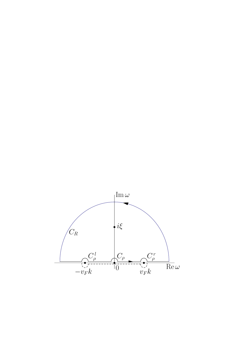
Figure 1: The contour of integration $C$ in the upper half-plane of complex frequency consisting of the real frequency axis, the semicircle $C_{R}$ of an infinitely large radius $R$, the semicircles $C_{\rho}^{\,l}$ and $C_{\rho}^{\,r}$ of the infinitely small radii $\rho$ around the branch points at $\omega=\mp v_{F}k$, and the semicircle $C_{\rho}$ of an infinite small radius $\rho$ around the double pole at $\omega=0$. The lower edge of the branch cut is shown by the dashed line.

Inside of the contour $C$ the function under the integral in Eq. (50) possesses the single simple pole at the point $\omega=i\xi$ of the imaginary frequency axis. Because of this, the integral (50) is calculated by using the Cauchy’s residue theorem

$$\int_{C}\frac{\omega[{\varepsilon}{(\omega,k)}-1]}{\omega^{2}+\xi^{2}}d\omega=2\pi i{\rm Res}{{\vphantom{\Bigl{(}}}_{\omega=i\xi}}\frac{\omega[{\varepsilon}{(\omega,k)}-1]}{\omega^{2}+\xi^{2}}$$

$$~{}~{}~{}~{}~{}~{}~{}~{}~{}~{}~{}~{}~{}~{}=\pi i[{\varepsilon}(i\xi,k)-1].$$ (51)

The integral on the left-hand side of Eq. (51) takes different values for ${\varepsilon}{(\omega,k)}={\varepsilon}^{\rm Tr}{(\omega,k)}$ and ${\varepsilon}{(\omega,k)}={\varepsilon}^{\rm L}{(\omega,k)}$. We begin with the first option and consider

$$H^{\rm Tr}(\xi,k)=\int_{C}\frac{\omega[{\varepsilon}^{\rm Tr}{(\omega,k)}-1]}{\omega^{2}+\xi^{2}}d\omega.$$ (52)

The quantity $H^{\rm Tr}(\xi,k)$ can be presented as the sum of the integrals along the real frequency axis from $-\infty$ to $+\infty$ and along the contours $C_{\rho}^{\,l}$, $C_{\rho}$, $C_{\rho}^{\,r}$, and $C_{R}$. In so doing, the contour $C_{R}$ should be bypassed in the positive direction (i.e., counter clockwise) whereas the semicircles $C_{\rho}^{\,l}$, $C_{\rho}$, and $C_{\rho}^{\,r}$ are bypassed in the negative direction (i.e., clockwise).

It is easily seen that the integral along the contour $C_{R}$ vanishes. Let us calculate

$$H_{C_{\rho}}^{\rm Tr}(\xi,k)=\int_{C_{\rho}}\frac{\omega[{\varepsilon}^{\rm Tr}{(\omega,k)}-1]}{\omega^{2}+\xi^{2}}d\omega,$$ (53)

where ${\varepsilon}^{\rm Tr}{(\omega,k)}-1$ is explicitly defined by the first line in Eq. (16). Substituting this explicit expression in Eq. (53), one obtains

$$H_{C_{\rho}}^{\rm Tr}(\xi,k)=-\frac{\pi\alpha kc}{2}\int_{C_{\rho}}\frac{\sqrt{b^{2}-\omega^{2}}\,d\omega}{\omega(\omega^{2}+\xi^{2})}.$$ (54)

The semicircle $C_{\rho}$ can be presented in the form $\omega=\rho e^{i\varphi}$ where $\varphi$ varies from $\pi$ to 0. Then Eq. (54) is rewritten as

$$H_{C_{\rho}}^{\rm Tr}(\xi,k)=-i\frac{\pi\alpha kc}{2}\int_{\pi}^{0}\frac{\sqrt{b^{2}-\rho^{2}e^{2i\varphi}}}{\rho^{2}e^{2i\varphi}+\xi^{2}}d\varphi$$

$$~{}~{}~{}{\,-\!\!\!\longrightarrow_{\vphantom{4mm}{}_{\rho\to 0}}{\ }}\>i\frac{\pi\alpha kc}{2}\int_{0}^{\pi}\frac{b}{\xi^{2}}d\varphi=i\frac{\pi^{2}\alpha kcb}{2\xi^{2}}.$$ (55)

In the Appendix B it is proven that

$$\int_{C_{\rho}^{\,l}}\!\!\frac{\omega[{\varepsilon}^{\rm Tr}{(\omega,k)}-1]}{\omega^{2}+\xi^{2}}d\omega=\int_{C_{\rho}^{\,r}}\!\!\frac{\omega[{\varepsilon}^{\rm Tr}{(\omega,k)}-1]}{\omega^{2}+\xi^{2}}d\omega=0,$$ (56)

i.e., the branch points $\omega=\pm v_{F}k$ do not contribute to the result. Substituting Eqs. (55) and (56) in Eq. (51) written for ${\varepsilon}{(\omega,k)}={\varepsilon}^{\rm Tr}{(\omega,k)}$, we find

$${\varepsilon}^{\rm Tr}(i\xi,k)-1=-\frac{i}{\pi}\mathchoice{{\vbox{\hbox{$\textstyle-$}}\kern-4.86108pt}}{{\vbox{\hbox{$\scriptstyle-$}}\kern-3.25pt}}{{\vbox{\hbox{$\scriptscriptstyle-$}}\kern-2.29166pt}}{{\vbox{\hbox{$\scriptscriptstyle-$}}\kern-1.875pt}}\!\int_{-\infty}^{\infty}\frac{\omega[{\varepsilon}^{\rm Tr}{(\omega,k)}-1]}{\omega^{2}+\xi^{2}}d\omega+\frac{\pi\alpha k^{2}cv_{F}}{2\xi^{2}}.$$ (57)

Taking into account that the following integrals of the odd functions of $\omega$ vanish

$$\mathchoice{{\vbox{\hbox{$\textstyle-$}}\kern-4.86108pt}}{{\vbox{\hbox{$\scriptstyle-$}}\kern-3.25pt}}{{\vbox{\hbox{$\scriptscriptstyle-$}}\kern-2.29166pt}}{{\vbox{\hbox{$\scriptscriptstyle-$}}\kern-1.875pt}}\!\int_{0}^{\infty}\frac{\omega\,d\omega}{\omega^{2}+\xi^{2}}=\mathchoice{{\vbox{\hbox{$\textstyle-$}}\kern-4.86108pt}}{{\vbox{\hbox{$\scriptstyle-$}}\kern-3.25pt}}{{\vbox{\hbox{$\scriptscriptstyle-$}}\kern-2.29166pt}}{{\vbox{\hbox{$\scriptscriptstyle-$}}\kern-1.875pt}}\!\int_{0}^{\infty}\frac{\omega{\rm Re}\,{\varepsilon}^{\rm Tr}{(\omega,k)}}{\omega^{2}+\xi^{2}}d\omega=0,$$ (58)

we rewrite Eq. (57) in the form

$${\varepsilon}^{\rm Tr}(i\xi,k)-1=\frac{2}{\pi}\mathchoice{{\vbox{\hbox{$\textstyle-$}}\kern-4.86108pt}}{{\vbox{\hbox{$\scriptstyle-$}}\kern-3.25pt}}{{\vbox{\hbox{$\scriptscriptstyle-$}}\kern-2.29166pt}}{{\vbox{\hbox{$\scriptscriptstyle-$}}\kern-1.875pt}}\!\int_{0}^{\infty}\frac{\omega{\rm Im}\,{\varepsilon}^{\rm Tr}{(\omega,k)}}{\omega^{2}+\xi^{2}}d\omega+\frac{\pi\alpha k^{2}cv_{F}}{2\xi^{2}},$$ (59)

which is the final form of the dispersion relation expressing ${\varepsilon}^{\rm Tr}(i\xi,k)$ via ${\rm Im}\,{\varepsilon}^{\rm Tr}{(\omega,k)}$. The last term on the right-hand side of the Eq. (59) originates from the double pole of ${\varepsilon}^{\rm Tr}{(\omega,k)}$ at zero frequency.

We are coming now to the longitudinal dielectric permittivity of graphene ${\varepsilon}^{\rm L}{(\omega,k)}$ and consider

$$H^{\rm L}(\xi,k)=\int_{C}\!\!\frac{\omega[{\varepsilon}^{\rm L}{(\omega,k)}-1]}{\omega^{2}+\xi^{2}}d\omega,$$ (60)

where the contour $C$ is shown in Fig. 1. The integral (60) is again presented as the sum of the integrals along the real frequency axis and along the contours $C_{\rho}^{\,l}$, $C_{\rho}$, $C_{\rho}^{\,r}$, and $C_{R}$ with the vanishing integral $H_{C_{R}}^{\rm L}$ along the latter in the limiting case $R\to\infty$.

For the dielectric permittivity ${\varepsilon}^{\rm L}{(\omega,k)}$ given by the first line of Eq. (15), the point $\omega=0$ is regular. Because of this

$$H_{\rho}^{\rm L}(\xi,k)=\int_{C_{\rho}}\!\!\frac{\omega[{\varepsilon}^{\rm L}{(\omega,k)}-1]}{\omega^{2}+\xi^{2}}d\omega{\,-\!\!\!\longrightarrow_{\vphantom{4mm}{}_{\rho\to 0}}{\ }}0.$$ (61)

The explicit calculation using Eq. (15) confirms this conclusion.

According to Eq. (15), at the branch points $\omega=\pm v_{F}k$ the permittivity ${\varepsilon}^{\rm L}{(\omega,k)}$ diverges by taking the real and complex values depending on whether the approach to a singular point along the real frequency axis occurs from the smaller or larger in magnitude values of frequency. In spite of this fact, as shown in the Appendix B,

$$\int_{C_{\rho}^{\,l}}\!\!\frac{\omega[{\varepsilon}^{\rm L}{(\omega,k)}-1]}{\omega^{2}+\xi^{2}}d\omega=\int_{C_{\rho}^{\,r}}\!\!\frac{\omega[{\varepsilon}^{\rm L}{(\omega,k)}-1]}{\omega^{2}+\xi^{2}}d\omega=0,$$ (62)

i.e., the branch points again do not contribute to the result.

Thus, using Eq. (51) written in this case for ${\varepsilon}^{\rm L}{(\omega,k)}$, one obtains

$${\varepsilon}^{\rm L}(i\xi,k)-1=-\frac{i}{\pi}\mathchoice{{\vbox{\hbox{$\textstyle-$}}\kern-4.86108pt}}{{\vbox{\hbox{$\scriptstyle-$}}\kern-3.25pt}}{{\vbox{\hbox{$\scriptscriptstyle-$}}\kern-2.29166pt}}{{\vbox{\hbox{$\scriptscriptstyle-$}}\kern-1.875pt}}\!\int_{-\infty}^{\infty}\!\!\frac{\omega[{\varepsilon}^{\rm L}{(\omega,k)}-1]}{\omega^{2}+\xi^{2}}d\omega.$$ (63)

With the help of Eq. (58), where ${\rm Re}\,{\varepsilon}^{\rm Tr}{(\omega,k)}$ is replaced with ${\rm Re}\,{\varepsilon}^{\rm L}{(\omega,k)}$, this equation can be rewritten in the form

$${\varepsilon}^{\rm L}(i\xi,k)-1=\frac{2}{\pi}\mathchoice{{\vbox{\hbox{$\textstyle-$}}\kern-4.86108pt}}{{\vbox{\hbox{$\scriptstyle-$}}\kern-3.25pt}}{{\vbox{\hbox{$\scriptscriptstyle-$}}\kern-2.29166pt}}{{\vbox{\hbox{$\scriptscriptstyle-$}}\kern-1.875pt}}\!\int_{0}^{\infty}\!\!\frac{\omega{\rm Im}\,{\varepsilon}^{\rm L}{(\omega,k)}}{\omega^{2}+\xi^{2}}d\omega,$$ (64)

which is the standard form of the dispersion relation valid for the response functions which are regular at zero frequency. Thus, the presence of the branch points and respective cut shown in Fig. 1 in the case of graphene makes no impact on the form of dispersion relations. Because of this, the statement that the dielectric permittivity has no singular points on the real frequency axis with the possible exception of only the coordinate origin 30 is, broadly speaking, inapplicable in the presence of spatial dispersion.

VI Conclusions and discussion of implications to the Casimir effect

In the foregoing, we have investigated the spatially nonlocal longitudinal and transverse dielectric permittivities of graphene expressed via the polarization tensor based on the first principles of quantum field theory. It was shown that at zero frequency the longitudinal permittivity is the regular function whereas the transverse one possesses a double pole for any nonzero wave vector. The obtained expressions are valid for any relationship between the frequency and the wave vector and, thus, describe the electromagnetic response of graphene to both the on-the-mass-shell and off-the-mass-shell fields.

According to our results, both the transverse and longitudinal permittivities of graphene are the analytic functions in the upper half-plane of complex frequency and satisfy the dispersion (Kramers-Kronig) relations for their real and imaginary parts for any value of the wave vector. In doing so, the dispersion relation for the transverse permittivity contains the additional term originating from the presence of a double pole at zero frequency, whereas the longitudinal permittivity satisfies the standard dispersion relation valid for dielectric materials. We have also obtained the dispersion relations expressing the dielectric permittivities of graphene along the imaginary frequency axis via their imaginary parts.

It was shown that the form of dispersion relations for the response functions of graphene is unaffected by a presence of the branch points whose position on the real frequency axis depends on the magnitude of the wave vector. We emphasize that the dispersion relations express the principle of causality and are valid for any function which is analytic in the upper half-plane of complex frequency. An application region of some function, satisfying the dispersion relations, in the theoretical description of a definite physical phenomenon is a different matter. However, the spatially nonlocal dielectric permittivities of graphene considered above are derived on the basis of first principles of quantum field theory in the framework of the Dirac model using the polarization tensor. Because of this, in the application region of this model, their specific features, including the presence of a double pole at zero frequency, are of doubtless physical significance.

As discussed in Sec. I, the experimental data on measuring the Casimir interaction in graphene systems are in good agreement with theoretical predictions of the Lifshitz theory when describing the electromagnetic response of graphene by means of the polarization tensor 20 ; 21 ; 22 ; 23 . The Lifshitz theory using the polarization tensor was also found in perfect agreement with the third law of thermodynamics (the Nernst heat theorem) 52 ; 53 . However, the predictions of the Lifshitz theory for metallic test bodies were found in disagreement with the measurement data and with the Nernst heat theorem when the response of metals at low frequencies is described by the dissipative Drude model. An agreement is restored when using the dissipationless plasma model at low frequencies where it should not work.

The meaning of disagreement of the fundamental Lifshitz theory with the measurement data should not be underestimated. Sometimes in the literature the following formulations are used: “experimental measurements of the Casimir interaction between two metallic objects… show a better agreement with the theoretical prediction using the plasma model than with that of the Drude model” 54 or “somewhat surprisingly, the less realistic dissipationless plasma model is in better agreement with experiment than the Drude model” 34 . In several precision Casimir experiments, however, the Drude model was excluded at the confidence level up to 99.9% (see Refs. 24 ; 25 for a review). Moreover, in the differential force measurement, where the theoretical predictions using the Drude and the plasma models differ by up to a factor of 1000, the Drude model was conclusively excluded, whereas the plasma model was shown to be in agreement with the measurement data 55 . Thus, the experimental situation demonstrates not a better or worse agreement, but an exclusion of the description by means of the Drude model and an agreement with the description given by the plasma model.

Although a neglect by the dissipation of conduction electrons at low frequencies cannot be considered as a satisfactory resolution of the problem, one should, nevertheless, admit that the plasma model has some important physical property which is missing in the Drude model. The lesson of graphene suggests that this property is the double pole at zero frequency which appears for graphene only at a nonzero wave vector, i.e., only with account of the spatial dispersion. This conclusion is in line with the spatially nonlocal phenomenological permittivities of metals suggested in Refs. 43 ; 44 ; 45 ; 46 , which are almost coinciding with the Drude model for the on-the-mass-shell fields but deviate from it for the fields off the mass shell and possess the double pole at zero frequency.

Recently the experimental test for the response of metals to the low-frequency s-polarized fields off the mass shell was suggested 56 ; 57 . It is based on measuring the magnetic field of a magnetic dipole oscillating in the proximity of metallic plate. The point is that most of the experiments confirming the validity of the Drude model were performed in the area of the propagating waves on the mass shell. As to the area of the s-polarized off-the-mass-shell waves, it remains little explored. Thus, the available information for the surface plasmon polaritons is restricted to only the area of p-polarized waves off the mass shell 58 . The total internal reflection technique makes it possible to examine the response of metals to the off-the-mass-shell fields, but for $k$ only slightly exceeding $\omega/c$ 59 ; 60 ; 61 . The methods used in the near field optical microscopy to surpass the diffraction limit 62 ; 63 are also more suitable for the p-polarized waves off the mass shell 64 .

One can conclude that the already available information concerning the response functions of graphene obtained on the solid basis of quantum field theory should be used for a reanalysis of the low-frequency electromagnetic response of metals in the area of s-polarized waves off the mass shell where the necessary experimental information is missing. In this respect, it seems prospective to continue investigation of the 3D Dirac materials 65 and to generalize the obtained results for the case of more complicated physical systems such as real metals.

Appendix A Involved integrals

Here, we calculate the integrals used in Sec. IV. Thus, the integral which appears in Eq. (32) is

$$I_{1}=\int_{-b}^{b}\frac{dx\sqrt{b^{2}-x^{2}}}{x-\omega}.$$ (A1)

Using the result 1.2.53(9) in Ref. 51 , one can present this integral in the form

$$I_{1}=-\int_{-b}^{b}\frac{xdx}{\sqrt{b^{2}-x^{2}}}-\omega\int_{-b}^{b}\frac{dx}{\sqrt{b^{2}-x^{2}}}$$

$$~{}~{}~{}+(b^{2}-\omega^{2})\int_{-b}^{b}\frac{dx}{(x-\omega)\sqrt{b^{2}-x^{2}}}$$ (A2)

$$~{}~{}~{}=-\pi\omega+(b^{2}-\omega^{2})\int_{-b}^{b}\frac{dx}{(x-\omega)\sqrt{b^{2}-x^{2}}}.$$

The integral entering Eq. (A2) is rearranged to the form

$$\int_{-b}^{b}\frac{dx}{(x-\omega)\sqrt{b^{2}-x^{2}}}=\int_{-b}^{0}\frac{dx}{(x-\omega)\sqrt{b^{2}-x^{2}}}$$

$$~{}~{}~{}~{}~{}~{}~{}~{}~{}~{}~{}~{}+\int_{0}^{b}\frac{dx}{(x-\omega)\sqrt{b^{2}-x^{2}}}.$$ (A3)

By changing the sign of the integration variable in the first integral on the right-hand side of Eq. (A3), we easily obtain

$$\int_{-b}^{b}\frac{dx}{(x-\omega)\sqrt{b^{2}-x^{2}}}=-2\omega\int_{0}^{b}\frac{dy}{(\omega^{2}-y^{2})\sqrt{b^{2}-y^{2}}}.$$ (A4)

The last integral can be evaluated with the help of 1.2.50(10) in Ref. 51 with the result

$$\int_{-b}^{b}\frac{dx}{(x-\omega)\sqrt{b^{2}-x^{2}}}=-2\omega\left\{\begin{array}[]{ll}0,&|\omega|<b,\\ \frac{\pi}{2|\omega|\sqrt{\omega^{2}-b^{2}}},&|\omega|>b.\end{array}\right.$$ (A5)

Substituting this result in Eq. (A2) and taking into account that $\omega/|\omega|=1$ for $\omega>0$ and $\omega/|\omega|=-1$ for $\omega<0$, we arrive at

$$I_{1}=\left\{\begin{array}[]{ll}-\pi\omega,&|\omega|<b,\\ -\pi\omega+\pi\sqrt{\omega^{2}-b^{2}},&\omega>b,\\ -\pi\omega-\pi\sqrt{\omega^{2}-b^{2}},&\omega<-b.\end{array}\right.$$ (A6)

The second integral which appears in Eq. (32)

$$I_{2}=\int_{-b}^{b}\!dx\frac{b-\sqrt{b^{2}-x^{2}}}{x^{2}}$$ (A7)

is a more simple one. By multiplying the numerator and denominator by $b+\sqrt{b^{2}-x^{2}}$, one can rearrange it to the form

$$I_{2}=\int_{-b}^{b}\frac{dx}{b+\sqrt{b^{2}-x^{2}}}=2\int_{0}^{b}\frac{dx}{b+\sqrt{b^{2}-x^{2}}}.$$ (A8)

Introducing the integration variable $y=\sqrt{b^{2}-x^{2}}$, we obtain

$$I_{2}=2\int_{0}^{b}\frac{ydy}{(y+b)\sqrt{b^{2}-y^{2}}}$$ (A9)

$$~{}~{}=2\int_{0}^{b}\frac{dy}{\sqrt{b^{2}-y^{2}}}-2b\int_{0}^{b}\frac{dy}{(y+b)\sqrt{b^{2}-y^{2}}}$$

$$~{}~{}=2\arcsin\left.\frac{y}{b}\right|_{0}^{b}+2\left.\sqrt{\frac{b-y}{b+y}}\right|_{0}^{b}=\pi-2.$$

Appendix B Branch points

Here, we calculate the integrals of the form of $H^{\rm Tr}(\xi,k)$ and $H^{\rm L}(\xi,k)$ in Eqs. (52) and (60) along the semicircles $C_{\rho}^{\,l}$ and $C_{\rho}^{\,r}$ around the branch points $\omega=\mp v_{F}k=\mp b$, respectively (see Fig. 1). We begin with

$$H_{C_{\rho}^{\,l}}^{\rm Tr}(\xi,k)=\int_{C_{\rho}^{\,l}}\frac{\omega[{\varepsilon}^{\rm Tr}{(\omega,k)}-1]}{\omega^{2}+\xi^{2}}\,d\omega.$$ (B1)

The semicircle $C_{\rho}^{\,l}$ bypassed in the negative direction can be described as $\omega=-b+\rho e^{i\varphi}$ where $\varphi$ varies from $\pi$ to 0. The permittivity ${\varepsilon}^{\rm Tr}{(\omega,k)}$ is given by the second and first lines in Eq. (16) when $\varphi$ varies from $\pi$ to $\pi/2$ and from $\pi/2$ and 0, respectively. Substituting these expressions in Eq. (B1) and using the equation of a semicircle, one finds

$$H_{C_{\rho}^{\,l}}^{\rm Tr}(\xi,k)=\frac{\pi\alpha kc}{2}\rho$$ (B2)

$$~{}\times\left\{\int_{\pi}^{\pi/2}d\varphi\frac{e^{i\varphi}\sqrt{(-b+\rho e^{i\varphi})^{2}-b^{2}}}{(-b+\rho e^{i\varphi})[(-b+\rho e^{i\varphi})^{2}+\xi^{2}]}\right.$$

$$~{}-i\left.\int_{\pi/2}^{0}d\varphi\frac{e^{i\varphi}\sqrt{b^{2}-(-b+\rho e^{i\varphi})^{2}}}{(-b+\rho e^{i\varphi})[(-b+\rho e^{i\varphi})^{2}+\xi^{2}]}\right\}.$$

From this equation it is seen that

$$H_{C_{\rho}^{\,l}}^{\rm Tr}(\xi,k){\,-\!\!\!\longrightarrow_{\vphantom{4mm}{}_{\rho\to 0}}{\ }}0.$$ (B3)

For the second branch point, we consider the integral

$$H_{C_{\rho}^{\,r}}^{\rm Tr}(\xi,k)=\int_{C_{\rho}^{\,r}}\frac{\omega[{\varepsilon}^{\rm Tr}{(\omega,k)}-1]}{\omega^{2}+\xi^{2}}\,d\omega,$$ (B4)

where the semicircle is described as $\omega=b+\rho e^{i\varphi}$ and, again, $\varphi$ varies from $\pi$ to 0. Here, however, the permittivity ${\varepsilon}^{\rm Tr}{(\omega,k)}$ is given by the first and second lines of Eq. (16) when $\varphi$ varies from $\pi$ to $\pi/2$ and from $\pi/2$ and 0, respectively. Substituting these expressions in Eq. (B4) and repeating the same calculation as above using the equation of a semicircle, we obtain

$$H_{C_{\rho}^{\,r}}^{\rm Tr}(\xi,k){\,-\!\!\!\longrightarrow_{\vphantom{4mm}{}_{\rho\to 0}}{\ }}0,$$ (B5)

i.e., Eq. (56) in the main text is proven.

Now we consider the quantity

$$H_{C_{\rho}^{\,l}}^{\rm L}(\xi,k)=\int_{C_{\rho}^{\,l}}\frac{\omega[{\varepsilon}^{\rm L}{(\omega,k)}-1]}{\omega^{2}+\xi^{2}}\,d\omega$$ (B6)

related to the longitudinal permittivity of graphene. In this case the permittivity is given by Eq. (15), i.e., it diverges at the branch points $\omega=\mp b$. In the vicinity of the branch point $\omega=-b$ under consideration now, ${\varepsilon}^{\rm L}{(\omega,k)}$ is given by the second and first lines in Eq. (15) when $\varphi$ varies from $\pi$ to $\pi/2$ and from $\pi/2$ and 0, respectively. Substituting these expressions in Eq. (B6) and using the equation of a semicircle $\omega=-b+\rho e^{i\varphi}$, we find

$$H_{C_{\rho}^{\,l}}^{\rm L}(\xi,k)=\frac{\pi\alpha kc}{2}\left\{\int_{\pi}^{\pi/2}d\varphi\frac{\rho e^{i\varphi}(-b+\rho e^{i\varphi})}{\sqrt{(-b+\rho e^{i\varphi})^{2}-b^{2}}[(-b+\rho e^{i\varphi})^{2}+\xi^{2}]}\right.$$

$$~{}+i\left.\int_{\pi/2}^{0}d\varphi\frac{\rho e^{i\varphi}(-b+\rho e^{i\varphi})}{\sqrt{b^{2}-(-b+\rho e^{i\varphi})^{2}}[(-b+\rho e^{i\varphi})^{2}+\xi^{2}]}\right\}.$$ (B7)

In the limiting case when $\rho$ goes to zero, Eq. (B7) reduces to

$$\lim_{\rho\to 0}H_{C_{\rho}^{\,l}}^{\rm L}(\xi,k)=-\frac{\pi\alpha kcb}{2(b^{2}+\xi^{2}}$$ (B8)

$$~{}\times\left\{\int_{\pi}^{\pi/2}\!e^{i\varphi}\lim_{\rho\to 0}\frac{\rho}{\sqrt{(-b+\rho e^{i\varphi})^{2}-b^{2}}}d\varphi\right.$$

$$~{}+i\left.\int_{\pi/2}^{0}\!e^{i\varphi}\lim_{\rho\to 0}\frac{\rho}{\sqrt{b^{2}-(-b+\rho e^{i\varphi})^{2}}}d\varphi\right\}.$$

The limits under the sign of these integrals can be
easily calculated using the l’Hôpital’s rule. For example,

$$\lim_{\rho\to 0}\frac{\rho}{\sqrt{b^{2}-(-b+\rho e^{i\varphi})^{2}}}=-\lim_{\rho\to 0}\frac{\sqrt{b^{2}-(-b+\rho e^{i\varphi})^{2}}}{(-b+\rho e^{i\varphi})e^{i\varphi}}=0$$ (B9)

leading, due to Eq. (B8), to

$$\lim_{\rho\to 0}H_{C_{\rho}^{\,l}}^{\rm L}(\xi,k)=0.$$ (B10)

The second branch point $\omega=v_{F}k$ is considered in perfect analogy to the above with the same result

$$\lim_{\rho\to 0}H_{C_{\rho}^{\,r}}^{\rm L}(\xi,k)=\lim_{\rho\to 0}\int_{C_{\rho}^{\,r}}\frac{\omega[{\varepsilon}^{\rm L}{(\omega,k)}-1]}{\omega^{2}+\xi^{2}}\,d\omega=0.$$ (B11)

This concludes the proof of Eq. (62)

References

- (1) A. H. Castro Neto, F. Guinea, N. M. R. Peres, K. S. Novoselov, and A. K. Geim, The electronic properties of graphene, Rev. Mod. Phys. 81, 109 (2009).
- (2) Physics of Graphene, ed. H. Aoki and M. S. Dresselhaus (Springer, Cham, 2014).
- (3) M. I. Katsnelson, The Physics of Graphene (Cambridge University Press, Cambridge, 2020).
- (4) T. Zhu, M. Antezza, and J.-S. Wang, Dynamical polarizability of graphene with spatial dispersion, Phys. Rev. B 103, 125421 (2021).
- (5) M. I. Katsnelson, K. S. Novoselov, and A. K. Geim, Chiral tunnelling and the Klein paradox in graphene, Nat. Phys. 2, 620 (2006).
- (6) D. Allor, T. D. Cohen, and D. A. McGady, Schwinger mechanism and graphene, Phys. Rev. D 78, 096009 (2008).
- (7) C. G. Beneventano, P. Giacconi, E. M. Santangelo, and R. Soldati, Planar QED at finite temperature and density: Hall conductivity, Berry’s phases and minimal conductivity of graphene, J. Phys. A 42, 275401 (2009).
- (8) G. L. Klimchitskaya and V. M. Mostepanenko, Creation of quasiparticles in graphene by a time-dependent electric field, Phys. Rev. D 87, 125011 (2013).
- (9) I. Akal, R. Egger, C. Müller, and S. Villarba-Chávez, Low-dimensional approach to pair production in an oscillating electric field: Application to bandgap graphene layers, Phys. Rev. D 93, 116006 (2016).
- (10) I. Akal, R. Egger, C. Müller, and S. Villalba-Chávez, Simulating dynamically assisted production of Dirac pairs in gapped graphene monolayers, Phys. Rev. D 99, 016025 (2019).
- (11) A. Golub, R. Egger, C. Müller, and S. Villalba-Chávez, Dimensionality-Driven Photoproduction of Massive Dirac Pairs near Threshold in Gapped Graphene Monolayers, Phys. Rev. Lett. 124, 110403 (2020).
- (12) P. K. Pyatkovsky, Dynamical polarization, screening, and plasmons in gapped graphene, J. Phys.: Condens. Matter 21, 025506 (2009).
- (13) M. Bordag, I. V. Fialkovsky, D. M. Gitman, and D. V. Vassilevich, Casimir interaction between a perfect conductor and graphene described by the Dirac model, Phys. Rev. B 80, 245406 (2009).
- (14) I. V. Fialkovsky, V. N. Marachevsky, and D. V. Vassilevich, Finite-temperature Casimir effect for graphene, Phys. Rev. B 84, 035446 (2011).
- (15) M. Bordag, G. L. Klimchitskaya, V. M. Mostepanenko, and V. M. Petrov, Quantum field theoretical description for the reflectivity of graphene, Phys. Rev. D 91, 045037 (2015); 93, 089907(E) (2016).
- (16) M. Bordag, I. Fialkovskiy, and D. Vassilevich, Enhanced Casimir effect for doped graphene, Phys. Rev. B 93, 075414 (2016); 95, 119905(E) (2017).
- (17) H. B. G. Casimir, On the attraction between two perfectly conducting bodies, Proc. Kon. Ned. Akad. Wet. B 51, 793 (1948).
- (18) E. M. Lifshitz, The theory of molecular attractive forces between solids, Zh. Eksp. Teor. Fiz. 29, 94 (1955) [Sov. Phys. JETP 2, 73 (1956)].
- (19) E. M. Lifshitz and L. P. Pitaevskii, Statistical Physics, Part II (Pergamon, Oxford, 1980).
- (20) A. A. Banishev, H. Wen, J. Xu, R. K. Kawakami, G. L. Klimchitskaya, V. M. Mostepanenko, and U. Mohideen, Measuring of the Casimir force gradient from graphene on a SiO2 substrate, Phys. Rev. B 87, 205433 (2013).
- (21) G. L. Klimchitskaya, U. Mohideen, and V. M. Mostepanenko, Theory of the Casimir interaction for graphene-coated substrates using the polarization tensor and comparison with experiment, Phys. Rev. B 89, 115419 (2014).
- (22) M. Liu, Y. Zhang, G. L. Klimchitskaya, V. M. Mostepanenko, and U. Mohideen, Demonstration of Unusual Thermal Effect in the Casimir Force for Graphene, Phys. Rev. Lett. 126, 206802 (2021).
- (23) M. Liu, Y. Zhang, G. L. Klimchitskaya, V. M. Mostepanenko, and U. Mohideen, Experimental and theoretical investigation of the thermal effect in the Casimir interaction from graphene, Phys. Rev. B 104, 085436 (2021).
- (24) G. L. Klimchitskaya, U. Mohideen, and V. M. Mostepanenko, The Casimir force between real materials: Experiment and theory, Rev. Mod. Phys. 81, 1827 (2009).
- (25) M. Bordag, G. L. Klimchitskaya, U. Mohideen, and V. M. Mostepanenko, Advances in the Casimir Effect (Oxford University Press, Oxford, 2015).
- (26) L. M. Woods, D. A. R. Dalvit, A. Tkatchenko, P. Rodriguez-Lopez, A. W. Rodriguez, and R. Podgornik, Materials perspective on Casimir and van der Waals interactions, Rev. Mod. Phys. 88, 045003 (2016).
- (27) V. M. Mostepanenko, Casimir Puzzle and Conundrum: Discovery and Search for Resolution, Universe 7, 040084 (2021).
- (28) G. L. Klimchitskaya and V. M. Mostepanenko, Current status of the problem of thermal Casimir force, Int. J. Mod. Phys. A 37, 2241002 (2022).
- (29) G. L. Klimchitskaya and V. M. Mostepanenko, Kramers-Kronig relations and causality conditions for graphene in the framework of the Dirac model, Phys. Rev. D 97, 085001 (2018).
- (30) L. D. Landau, E. M. Lifshitz, and L. P. Pitaevskii, Electrodynamics of Continuous Media (Pergamon, Oxford, 1984).
- (31) V. A. Parsegian, Van der Waals Forces: A Handbook for Biologists, Chemists, Engineers, and Physicists (Cambridge University Press, Cambridge, 2005).
- (32) G. L. Klimchitskaya, U. Mohideen, and V. M. Mostepanenko, Kramers-Kronig relations for plasma-like permittivities and the Casimir force, J. Phys. A: Math. Theor. 40, F339 (2007).
- (33) I. Brevik and B. Shapiro, A critical discussion of different methods and models in Casimir effect, J. Phys. Commun. 6, 015005 (2022).
- (34) I. Brevik, B. Shapiro, and M. G. Silverinha, Fluctuational electrodynamics in and out of equilibrium, Int. J. Mod. Phys. A 37, 2241012 (2022).
- (35) J. Lindhard, On the properties of a gas of charged particles, Dan. Mat. Fys. Medd. 28, 1 (1954).
- (36) Z. H. Levine and E. Cockayne, The Pole Term in Linear Response Theory: An Example From the Transverse Response of the Electron Gas, J. Res. Natl. Inst. Stand. Technol. 113, 299 (2008).
- (37) G. Barton, Introduction to Dispersion Techniques in Field Theory (W.A. Benjamin, New York, 1965).
- (38) D. Drechsel, B. Pasquini, and M. Vanderhaeghen, Dispersion relations in real and virtual Compton scattering, Phys. Rep. 378, 99 (2003).
- (39) S. Coleman and H. J. Thun, On the Prosaic Origin of the Double Poles in the Sine-Gordon S-Matrix, Commun. Math. Phys. 61, 31 (1978).
- (40) W. Vanroose, P. Van Leuven, F. Arickx, and J. Broeckhove, Double poles of the S-matrix in a two-channel model, J. Phys. A: Math. Gen. 30, 5543 (1997).
- (41) N. J. Kylstra and C. J. Joachain, Double poles of the S matrix in laser-assisted electron-atom scattering, Phys. Rev. A 57, 412 (1998).
- (42) W. Vanroose, Double pole of the S matrix in a double-well system, Phys. Rev. A 64, 062708 (2001).
- (43) G. L. Klimchitskaya and V. M. Mostepanenko, An alternative response to the off-shell quantum fluctuations: A step forward in resolution of the Casimir puzzle, Eur. Phys. J. C 80, 900 (2020).
- (44) G. L. Klimchitskaya and V. M. Mostepanenko, Theory-experiment comparison for the Casimir force between metallic test bodies: A spatially nonlocal dielectric response, Phys. Rev. A 105, 012805 (2022).
- (45) G. L. Klimchitskaya and V. M. Mostepanenko, Casimir effect for magnetic media: Spatially nonlocal response to the off-shell quantum fluctuations, Phys. Rev. D 104, 085001 (2021).
- (46) G. L. Klimchitskaya and V. M. Mostepanenko, Casimir entropy and nonlocal response functions to the off-shell quantum fluctuations, Phys. Rev. D 103, 096007 (2021).
- (47) Bo E. Sernelius, Retarded interactions in graphene systems, Phys. Rev. B 85, 195427 (2012).
- (48) G. L. Klimchitskaya, V. M. Mostepanenko, and Bo E. Sernelius, Two approaches for describing the Casimir interaction with graphene: Density-density correlation function versus polarization tensor, Phys. Rev. B 89, 125407 (2014).
- (49) Bo E. Sernelius, Fundamentals of van der Waals and Casimir Interactions (Springer, Cham, 2018).
- (50) I. S. Gradshtein and I. M. Ryzhik, Table of Integrals, Series and Products (Academic Press, New York, 2007).
- (51) A. P. Prudnikov, Yu. A. Brychkov, and O. I. Marichev, Integrals and Series. Vol. 1. Elementary Functions (Gordon and Breach, New York, 1986).
- (52) G. L. Klimchitskaya and V. M. Mostepanenko, Nernst heat theorem for an atom interacting with graphene: Dirac model with nonzero energy gap and chemical potential, Phys. Rev. D 101, 116003 (2020).
- (53) G. L. Klimchitskaya and V. M. Mostepanenko, Quantum field theoretical description of the Casimir effect between two real graphene sheets and thermodynamics, Phys. Rev. D 102, 016006 (2020).
- (54) F. Intravaia, How modes shape Casimir physics, Int. J. Mod. Phys. A 37, 2241014 (2022).
- (55) G. Bimonte, D. López, and R. S. Decca, Isoelectronic determination of the thermal Casimir force, Phys. Rev. B 93, 184434 (2016).
- (56) G. L. Klimchitskaya, V. M. Mostepanenko, and V. B. Svetovoy, Probing the response of metals to low-frequency -polarized evanescent fields, Europhys. Lett. 139, 66001 (2022).
- (57) G. L. Klimchitskaya, V. M. Mostepanenko, and V. B. Svetovoy, Experimentum crucis for electromagnetic response of metals to evanescent waves and the Casimir puzzle, Universe 8, 574 (2022).
- (58) P. Törmä and W. L. Barnes, Strong coupling between surface plasmon polaritons and emitters: a review, Rep. Progr. Phys. 78, 013901 (2015).
- (59) W. Culshaw and D. S. Jones, Effect of a Metal Plate on Total Reflection, Proc. Phys. Soc. B 66, 859 (1953).
- (60) J. J. Brady, R. O. Brick, and V. D. Pearson, Penetration of Microwaves into the Rarer Medium in Total Reflection, J. Opt. Soc. Am. 50, 1080 (1960).
- (61) S. Zhu, A. W. Yu, D. Hawley, and R. Roy, Frustrated total internal reflection: A demonstration and review, Am. J. Phys. 54, 601 (1986).
- (62) J.-J. Greffet and R. Carminati, Image formation in near-field optics, Prog. Surf. Sci. 56, 133 (1997).
- (63) J. W. P. Hsu, Near-field scanning optical microscopy studies of electronic and photonic materials and devices, Mater. Sci. Engin: R: Reports 33, 1 (2001).
- (64) L. Aigouy, A. Lahrech, S. Grésillon, H. Cory, A. C. Boccara, and J. C. Rivoal, Polarization effects in apertureless scanning near-field optical microscopy: an experimental study, Opt. Lett. 24, 187 (1999).
- (65) M. Bordag, I. V. Fialkovsky, N. Khusnutdinov, and D. V. Vassilevich, Bulk contributions to Casimir interaction of Dirac materials, Phys. Rev. B 104, 195431 (2021).