MultiGain 2.0: MDP controller synthesis for multiple mean-payoff, LTL and steady-state constraints

Abstract

We present MultiGain 2.0, a major extension to the controller synthesis tool MultiGain, built on top of the probabilistic model checker PRISM. This new version extends MultiGain’s multi-objective capabilities, by allowing for the formal verification and synthesis of controllers for probabilistic systems with multi-dimensional long-run average reward structures, steady-state constraints, and linear temporal logic properties. Additionally, MultiGain 2.0 provides an approach for finding finite memory solutions and the capability for two- and three-dimensional visualization of Pareto curves to facilitate trade-off analysis in multi-objective scenarios.

1 Introduction

Markov decision processes

(MDP), e.g., [12], are the basic model for decision-making in uncertain environments. The policy synthesis problem is the problem of resolving the choices so that a given specification is satisfied. In verification, there are many types of properties considered; in this work, we focus on infinite-horizon properties. Firstly, Linear Temporal Logic (LTL) [11] is mainstream in verification [4]. It can express complex temporal relationships, abstracting from the concrete quantitative timing, e.g., after every request, there is a grant (not saying when exactly). Secondly, Steady-State Policy Synthesis (SS) [2] constrains the frequency with which states are visited, providing a more quantitative perspective. Recently, it has started receiving more attention also in AI planning [14, 3, 9]. Thirdly, rewards provide a classic framework for quantitative properties. In the setting of infinite horizon, a key role is played by the long-run average reward (LRA, a.k.a. mean payoff), e.g., [12], which constrains the reward gained on average per step.

Example 1

An example of an MDP with these specifications is shown below in Fig. 1. There is a non-trivial choice at the beginning, deciding, intuitively, in which set of states we shall be circulating forever. Such a set is called a maximum end component (MEC). Further, there is another choice in the middle MEC and a probabilistic transition in the right one. The LTL formula in the example specifies that whenever a red state occurs, it is followed by non-red ones until a green one occurs. This can be satisfied in all the MECs, they are so-called accepting MECs. The steady-state constraint determines that we stay in green states at least 60% of the time. Finally, the rewards are decorating the edges and then the average reward will be maximized in the middle MEC. If all specifications are considered together, the reward is maximized in the right MEC only, because of the SS constraint.

• linear temporal logic (LTL)

  $${\mathbf{G}}(\leavevmode\hbox to6.43pt{\vbox to6.43pt{\text{[drawing]}}}\implies{\mathbf{X}}(\neg\leavevmode\hbox to6.43pt{\vbox to6.43pt{\text{[drawing]}}}{\mathbf{U}}\leavevmode\hbox to6.43pt{\vbox to6.43pt{\text{[drawing]}}}))$$

• steady-state constraints (SS)

  $$\leavevmode\hbox to6.43pt{\vbox to6.43pt{\text{[drawing]}}}\geq 0.6$$

• long-run average reward (LRA)

  $$\lim_{n\to\infty}(\inf)\frac{1}{n}\sum_{i=1}^{n}{r}(A_{i})$$

Figure 1: An MDP and its heterogeneous specification

We consider MDP with the specifications combining all these three types, as introduced and theoretically solved in [9], using reduction to multi-dimensional long-run average reward and solved by linear programming (LP). Our tool synthesizes a policy maximizing the LRA reward among all policies, ensuring the LTL specification (with the given probability) and adhering to the steady-state constraints.

In summary, our contribution is as follows:

• We extend MultiGain to analyze an MDP with a heterogeneous LTL+SS+LRA specification for maximizing the long-run average reward under the LTL and steady-state constraints, as described in [9]. Additionally, we extend the specification and the algorithm to cater for further constraints. For example, satisfaction by policies that are deterministic (as in [15]), policies remaining in a single MEC, or policies with a bound on the size of their memory.

• We extend the syntax of the PRISM language slightly to accommodate the richer queries. We can also display two- and three-dimensional Pareto curves, to visualize the trade-offs.

• We conduct a series of experiments to demonstrate the scalability of the tool.

Related tools. To the best of our knowledge, there are no tools that can simultaneously handle multi-dimensional LRA reward computation, LTL, and steady-state specifications. There are, however, two tools that handle multi-dimensional LRA objectives: (i) the previous version of MultiGain implements this functionality through linear programming which is also compatible with the solution offered in [9] and implemented here; and (ii) STORM [13], which implements the same functionality more efficiently through value iteration. Additionally, the Partial Exploration Tool (PET) [10] includes an implementation for LRA reward analysis, by focusing on partial exploration of the state space. However, it does not account for additional objectives such as LTL or steady-state specifications. Furthermore, the work of [15] presents a solution concept for finding deterministic unichain policies under LTL and steady-state constraints, however, it does not include any reward structures.

2 Functionality

The main functionality of our tool is to answer multi-objective LRA queries constrained by LTL and steady-state specifications for MDPs and to synthesize a policy, if possible. We begin with an overview of the tool’s functionality, followed by a description of the various types of queries that are currently supported, including their syntax and semantics. Finally, we discuss additional functionalities that can be accessed via the command line interface, and highlight key attributes of our tool.

2.1 Workflow

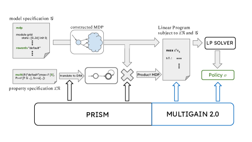
Figure 2: The workflow of MultiGain 2.0  from input specifications to output policy.

Our tool follows the workflow depicted in Fig. 2. As the input, it is given an MDP, defined in the standard PRISM language, and an infinite-horizon property, specified in an extension of PRISM’s property specification language that we developed. PRISM starts by constructing the MDP from the input file and translates the specified LTL property into a Deterministic Rabin Automaton (DRA). Then, it forms the product between the MDP and the DRA, also known as the product MDP, which is then passed as an input to the novel component of our tool. Here, an LP is constructed, following the methodology described in [9], and fed to an LP solver. Finally, after the LP is solved, MultiGain 2.0  extracts the solution from the solver and, if required, synthesizes a policy.

2.2 Application

Figure 1 An example instance of the adjusted grid world model.

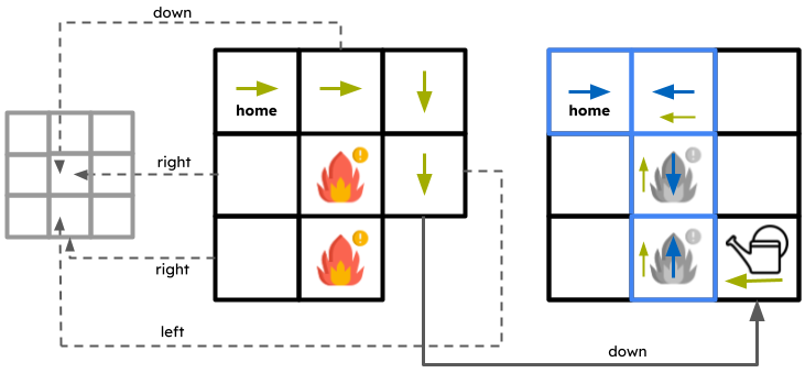
Figure 2 The computed product model and policy. The transient part of the policy is described with green arrows, the recurrent part with blue arrows. The blue framed state have positive switch probability from transient to recurrent behaviour.

Figure 3: Example application of MultiGain 2.0 to an adjusted grid world model (left) and the corresponding solution (right).

Example application. Fig. 3 shows an example computation of our tool on a grid world model. Grid world models have been used extensively for the performance evaluation of various MDP algorithms and tools in fields such as reinforcement learning [8], motion planning [5] and formal verification [15]. A grid world model is a two-dimensional grid of $N\times N$ states where an agent can traverse by using one of the four actions, left, down, up, right, available at each state. In the example considered, the model consists of 3 $\times$ 3 grid cells, and only actions which lead to another state may be chosen, i.e., no self-loop actions. Two cells are labeled "danger" and one cell is labeled "water_can" to indicate that they are on fire and the presence of a watering can, respectively. The initial state, labeled "home" is located in the top left cell.

The following shows the full query used for the computations in Fig. 3:

⬇

multi(R{"extinguish"}max=? [S], P>=1 [(! "danger") U "water_can"], S>=0.25 ["home"])

where the reward structure "extinguish" assigns a reward of 1 to the two fire states, intuitively encouraging the agent to repeatedly extinguish resurging flames. The LTL formula requires not to move onto any fire cell before collecting the watering can and the steady-state constraint implies staying home a sufficient amount of time in the long run.

Subject to this constraint, as discussed in Section 2.1 and shown on the right of Fig. 3, the product MDP model is constructed, and the maximized LRA reward of $0.5$ is returned. Intuitively, the product model consists of three copies of the grid, with a non-accepting MEC (gray grid on the left), which is reached when traversing to a fire cell before visiting the watering can, and the unique accepting MEC (right), reached when visiting the watering can cell first. The transient, recurrent and switching behavior of the policy is indicated by arrows in the product model in Fig. 3. After the transient part directly guides around the fires to the watering can it continues to traverse to any state with positive frequency in the long-run. At each such state the policy has a probability to switch to recurrent behaviour, which suggests to loop both on the fire and the home cells. It may be noticed that the recurrent part is disconnected, but the individual states with positive occupation measure are still reached by the policy.

2.3 Infinite-horizon properties

As described before, a multi-objective query for MultiGain 2.0  consists of the following specifications:

1. Long-run average: Two types of LRA properties can be specified: (i) a numerical property, which seeks to determine the maximum (or minimum) LRA achievable, or (ii) a Boolean property that determines whether the LRA crosses a certain threshold or not. In PRISM’s syntax, a numerical or a Boolean LRA property could be represented as R{"rewardStruct"}max=?[S] or R{"rewardStruct"}
   >=0.5[S] respectively.

2. LTL: The tool only supports a single Boolean query for LTL specifications, since multiple LTL formulae can be conjoined to form one formula. An example could look like P>=0.75 [G F "stateLabel"], which expresses that with probability $\geq 0.75$, states with the label stateLabel are reached infinitely often.

3. Steady-state: An SS property of type  S<=0.1 ["stateLabel"] requires that the steady-state probability distribution of the states with label stateLabel is bounded from above by $0.1$.

2.4 Syntax and semantics

As described in [9], there are several types of queries one can formulate by combining the properties discussed above. Moreover, as previously discussed, we extended PRISM’s syntax to allow for new types of queries using the following notation:

keyword ( $$[N,] prop_{1},prop_{2},\cdots,prop_{k}$$ )

where the keyword can be one among multi, mlessmulti, detmulti, or unichain and each $prop_{i}$ is an LRA, LTL, or SS property. Note that there can be only one LTL property in the syntax of a query. We now explain the semantics of the three different keywords.

2.4.1 Multi

The semantics of the multi keyword is similar to its meaning in PRISM and MultiGain, i.e., computing a policy that satisfies the conjunction of all the individual properties. Here, the type of result obtained depends on the number of numerical LRA properties. If there are no numerical properties, the query only consists of Boolean LRA, LTL, and SS properties and the result is either true or false, depending on whether all of them can be satisfied or not. In the case of a single numerical LRA property, the tool returns the maximum (or minimum) achievable value for that LRA reward while satisfying all of the other properties. When more than one numerical property is given, the tool approximates the corresponding Pareto curve while satisfying all of the other properties. Currently, the tool only supports the maximization of LRA rewards. An example of a multi query is shown below:

⬇

multi(R{"reward1"}max=? [S], R{"reward2"}max=? [S], R{"reward3"}>=0.5 [S], P>=0.75[G F "stateLabel1"], S>=0.5 ["stateLabel2"], S<=0.5["stateLabel2"])

• linear temporal logic (LTL)

  ${\mathbf{G}}{\mathbf{F}}$

• steady-state constraint (SS)

  ( , $1$, $1$)

Figure 4: An example MDP with LTL and steady-state constraints. Only policies visiting the accepting state less and less frequently satisfy both specifications, requiring unbounded memory for the information on a current run’s history.

The mlessmulti keyword, used in the previous version of our tool, solves a different problem in its current implementation. In general, a policy computed by the LP (i.e., a multi query) might visit the accepting states less and less often to satisfy the remaining constraints, thus requiring unbounded memory as seen in Fig. 4. Relaxing the LRA and SS specifications by an arbitrary factor $\delta>0$ lifts this restriction [9], such that a finite-memory policy exists for the model.

The implementation of a mlessmulti query addresses this problem from a different angle. It allows the user to specify an additional integer $N$, signifying the maximum number of steps in the long-run before an accepting state is revisited. The tool subsequently computes and outputs the resulting minimal factor $\delta$ to uniformly relax all steady-state specifications and long-run average rewards, with regards to this fixed accepting frequency. Hence, exporting the strategy yields a finite-memory policy, more specifically a 2-memory policy [9]. Note that due to the modified objective function it is not possible to define numerical LRA properties in a mlessmulti query. An example of a mlessmulti query is shown below:

⬇

mlessmulti(1000, R>=0.5 ["sLabel"], P>=1[G F "tLabel"], S>=1 ["sLabel"], S<=1["sLabel"])

2.4.2 Detmulti

Depending on the underlying model and property specification, the policy computed by the multi keyword may exhibit two significant characteristics. Firstly, it is typically non-deterministic, and secondly, the policy may require an infinite amount of memory to remember the current history. To address both of these issues, the unichain keyword implements the approach by [15], which is also based on a (integer) linear program. The resulting policy, which is defined over the original MDP rather than the product, is both deterministic and finite-memory. The detmulti queries may contain a single LTL property and arbitrarily many steady-state specifications. The result, other than an exportable policy, is a boolean value indicating whether a solution was found or not. An example of a detmulti query is shown below:

⬇

detmulti(P>=0.75 [(! "stateLabel1") U "stateLabel2"], S>=0.75 ["stateLabel3"], S<=1 ["stateLabel3"])

2.4.3 Unichain

We introduce the keyword unichain, which computes a unichain solution for the multi query, i.e., the recurrent run resides only in a single MEC, by exploring each MEC (or accepting MEC if an LTL specification is present) individually. The implementation concept follows the idea presented in [9, Section 6]. If no numerical LRA properties are specified, the tool explores the MECs until a unichain solution is found and outputs the corresponding boolean value. For a single numerical LRA property, our tool searches for the unichain solution maximizing (or minimizing) the reward structure and outputs the corresponding reward. Multiple numerical rewards are not allowed for this keyword, as this would result in comparing multiple Pareto curves. An example of a unichain query is shown below:

⬇

unichain((R{"reward1"}max=? [S], R{"reward2"}>=0.5 [S], P>=0.75[G F "stateLabel1"], S>=0.5 ["stateLabel2"], S<=0.5["stateLabel2"])

2.5 Interface

The tool is used via a command line interface, which requires the user to specify two files as input arguments, containing the model and the queries. The approximated Pareto curve can be exported to a file by using the flag –exportpareto. Furthermore, the tool includes a Python script that enables the visualization of Pareto frontiers with two or three dimensions. In Fig. 5, we show example plots of two- and three-dimensional Pareto frontiers. Moreover, for all queries except Pareto approximation, we provide the option to export the computed policy, which may have an unbounded memory, to a file in various formats.

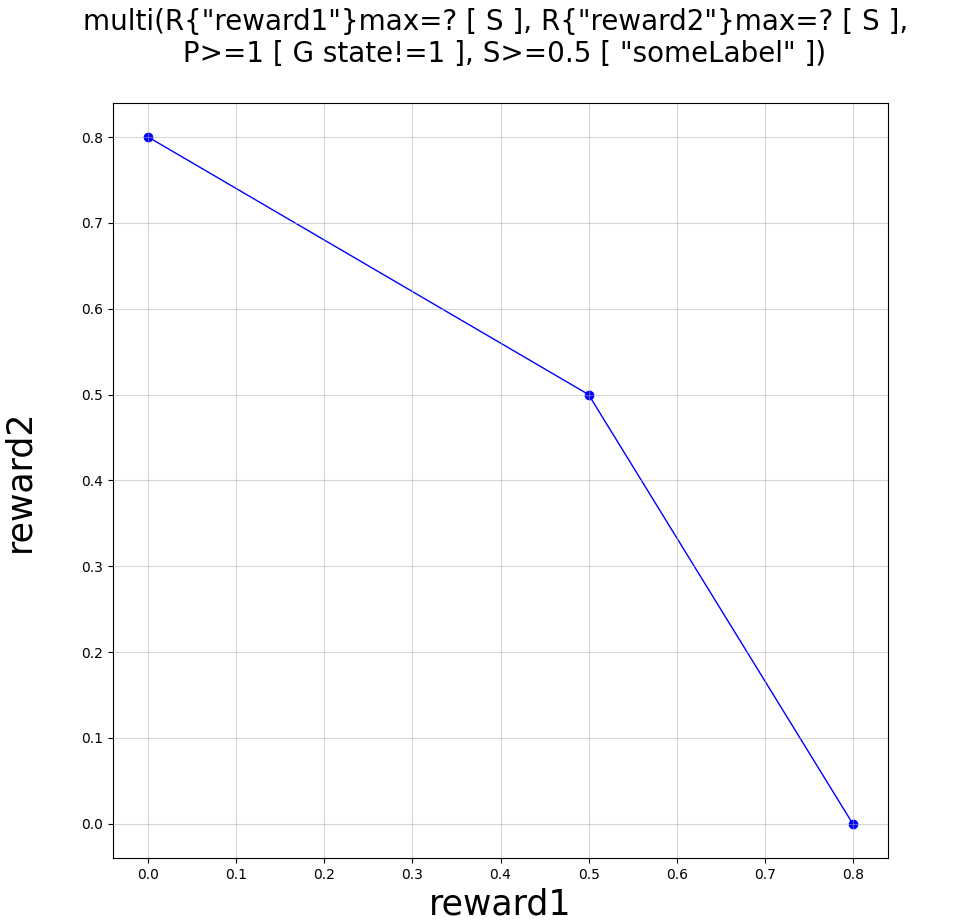
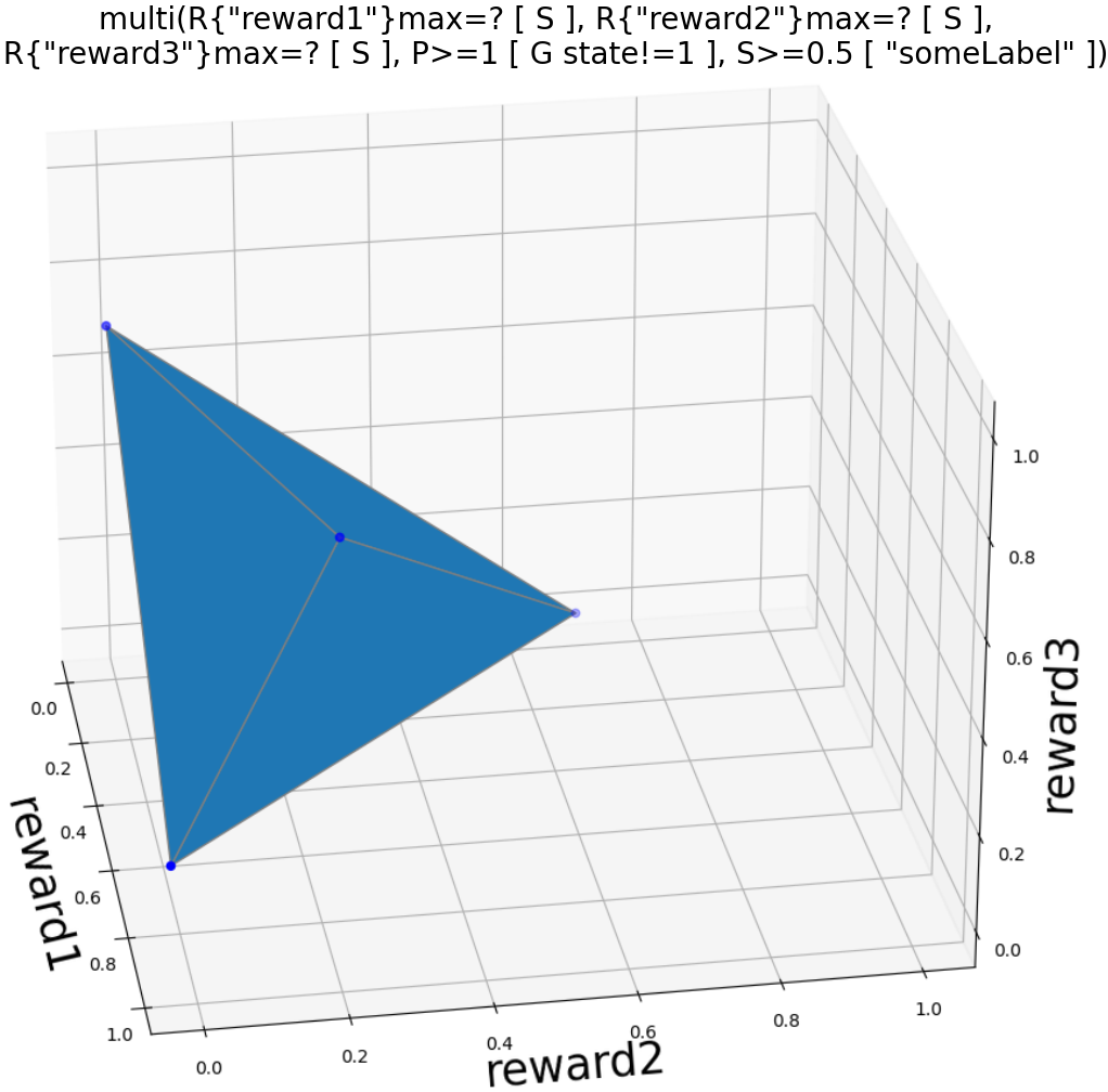
Figure 5: Example plots of approximated Pareto curves with 2 and 3 dimensions.

2.6 Key quality characteristics

In this section, we report on the quality of MultiGain 2.0  by highlighting some of its key characteristics.

Extensibility. The underlying LP solver implements a general interface and can thus be easily switched for every run. This implementation allows the simple extension and addition of further LP solvers. Currently, the tool supports the use of $\mathtt{lp\_solve}$ [1] and $\mathtt{Gurobi}$ [6]. After solving the LP, the tool extracts the solution from the solver and, if required, synthesizes a policy.

For approximating Pareto curves a new generic class has been implemented which takes as input a weight function, mapping weights to reward structures. This class lifts the Pareto curve approximation from MultiGain 2.0  so that other PRISM-based tools could utilize it. Furthermore, Pareto curves of any dimension can be approximated, contrary to the two-dimensional limit of the old implementation. Since the tool is implemented in the unifying approach of the PRISM pipeline, it can be extended at a variety of entry points, as seen in Fig. 2. For example, new deterministic automata could be implemented alongside the translation of the LTL and building the product model, without changing the tool’s core functionality.

Efficiency, reusability, and readability. The implementation of the unichain keyword leverages the reusability of preexisting LP solution to increase efficiency. For example, only one instance of the LP and the solver is created initially, and it is adjusted by adding and removing only a single constraint for each explored MEC. Therefore, the solver may resolve the adjusted LP with a warm start. Our tool further utilizes modern features of Java (e.g., streams, lambdas, etc.) to enhance comprehensibility.

3 Experimental Evaluation

In this section, we assess the performance of our tool in terms of its ability to solve the three types of queries described in Section 2.4. We conducted multiple experiments to evaluate the performance of our tool. We first discuss the experimental setup, followed by the technical details regarding our experiments, and then we give a detailed overview of our experimental results in Section 3.1. Note that due to space constraints we present only a subset of our experiments.

Experimental setup. Our evaluation consists of two parts: (i) the evaluation of the full property suite (LRA, SS, and LTL properties) using a grid world model; and (ii) a comparison of the performance on single objective LRA queries with the PET tool based on various QComp benchmarks [7].

Regarding the first part, the performance of our tool was evaluated on 20 randomly labeled instances of a grid world model of different sizes. Also, the reasons for choosing a grid world model are discussed in Section 2.

For the second part of our evaluation, we compared only the computation of single LRA rewards with the PET tool. This is because, to the best of our knowledge, there exist no other tools capable of computing general LRA rewards constrained with LTL and SS properties. The PET tool is the state-of-the-art PRISM-based implementation for solving single LRA rewards, and this comparison could potentially provide additional insight regarding the performance of our tool. Note that, we deliberately focused our evaluation on other PRISM-based tools, thereby excluding a comparison with STORM, since a previous comparison has already been conducted and STORM was shown to outperform MultiGain [13]. Moreover, the aim of the tool is not to become competitive on the specific task of mean-payoff analysis, but rather to provide an implementation for the analysis of the more complex specifications (also involving LTL and steady-state constraints), which no other tool can handle. Finally, the various models from the QComp Benchmark Set [7] were chosen based on their suitability for conducting long-run average experiments.

Table 1: Average running time (in seconds) over 20 randomly grid world labeled instances.

		Average running time for each grid
LTL	$\mathtt{R}^{\mathit{rew\_c}}_{\mathtt{max}=?}[\,\mathtt{S}\,]$ (LRA)	$4\times 4$	$16\times 16$	$32\times 32$	$64\times 64$
${\mathbf{G}}(\neg b)\land(GFb)$	$\times$	$0.186$	$0.302$	$0.543$	$1.251$
$({\mathbf{G}}{\mathbf{F}}a)\lor({\mathbf{F}}{\mathbf{G}}b)$	$\times$	$0.201$	$0.308$	$0.499$	$1.053$
$({\mathbf{F}}a)$$\mathbf{U}$$b$	$\times$	$0.167$	$0.264$	$0.537$	$1.438$
$({\mathbf{F}}a)\land({\mathbf{F}}b)\land({\mathbf{F}}c)$	$\times$	$0.209$	$0.439$	$1.319$	$4.258$
${\mathbf{G}}(\neg b)\land({\mathbf{G}}{\mathbf{F}}b)$	✓	$0.197$	$0.369$	$1.149$	$15.849$
$({\mathbf{G}}{\mathbf{F}}a)\lor({\mathbf{F}}{\mathbf{G}}b)$	✓	$0.202$	$0.363$	$0.929$	$9.222$
$({\mathbf{F}}a)$$\mathbf{U}$$b$	✓	$0.171$	$0.313$	$1.208$	$16.179$
$({\mathbf{F}}a)\land({\mathbf{F}}b)\land({\mathbf{F}}c)$	✓	$0.222$	$0.657$	$5.068$	$92.851$

Technical details. All experiments were performed on a computer with 8 GB of RAM and $4\times$ Intel®Core^TM i5-6200U CPU @ 2.30GHz processor, running Arch Linux, and each run was restricted to a 1 GB of RAM using $\mathtt{Gurobi}$ as the LP solver. We always used a precision of $\varepsilon=10^{-6}$. Each model was run 5 times and the average running time is recorded in the respective table. For the grid world model the average running time over 20 runs was recorded, as a countermeasure to the high variance of individual running times. The timeout threshold (T/O) was set to 5 minutes and all results are rounded to three decimal places.

3.1 Results

Table 2: Average running times (in seconds) and result values over 5 runs of each model.

Model	# States	# MECs	Solver time	Total time	Value	Total time (PET)	Value	Unichain	Value
$\mathtt{rabin}(3)$	27766	1	$13.944$	$16.001$	$0.857$	$10.938$	$0.857$	$15.173$	$0.857$
$\mathtt{mer}(3)$	15622	9451	$4.276$	$19.194$	$1.5$	$7.526$	$1.35$	T/O	T/O
$\mathtt{pacman}(10)$	6854	1010	$0.0536$	$0.902$	$0.780$	$1.692$	$0.78$	$6.955$	NaN
$\mathtt{pacman}(15)$	96894	3958	$1.18$	$13.353$	$0.995$	$3.066$	$0.995$	T/O	T/O
$\mathtt{virus}(3)$	809	1	$0.019$	$0.279$	$0.0$	$1.39$	$0.0$	$0.176$	$0.0$
$\mathtt{eajs}(500)$	93228	1	$10.678$	$12.455$	$3.637$	$209.2$	$3.27$	$11.877$	$3.637$
$\mathtt{eajs}(1000)$	193728	1	$46.845$	$49.62$	$3.637$	T/O	T/O	$49.066$	$3.637$

LRA+LTL+SS queries. In Table 1, the results for various multi queries that combine all three types of properties are presented. We distinguish between the queries which consist of an LRA property from those who do not, with the ✓and $\times$ symbols, respectively. Following the experiments in [15], the states were randomly partitioned into four equally-sized subsets and labeled with the atomic propositions $AP=\{a,b,c,d\}$ before each run of the tool. A reward structure $rew_{c}$ was also created that assigns a reward of 1 to every state with label $c$. Each run required each LTL formula to be fulfilled with a probability threshold of $\theta=0.5$ and steady-state constraints of $S\geq 0.01[$"$d$"$]$, $S\leq 0.5[$"$d$"$]$.

The results of the first set of our experiments (upper-half of Table 1), demonstrate the efficient performance of our tool with a maximum running time of $\approx$ 4 seconds for the largest grid world MDP model. The average running time of the second set of experiments, located in the bottom-half of Table 1, which also includes the maximization of the LRA of $rew\_c$ (denoted as $\mathtt{R}^{\mathit{rew\_c}}_{\mathtt{max}=?}[\,\mathtt{S}\,]$), does not experience any significant increase, as the size of the grid world model increases. In addition, the average running time remains at acceptable levels of $\approx 13$ seconds, for the first three LTL properties of the largest model considered. On the other hand, for the same model, an increase of $\approx 80$ seconds is observed when the last LTL property is considered. It is important to note that a similar increasing trend is also observed in the results of [15]. This increase can be attributed to the random generation procedure of the grid world instances, which might be biased towards certain types of models. Overall, the results show, that the tool scales well to reasonably-sized models, limited primarily by the LP solver, as can be observed from the average solving time in Table 2.

Single LRA queries. In Table 2, we compare the performance of our tool against the PET tool. For our tool, the LP solving and total model checking times are collected. Further, the unichain computation time and solution are shown with respect to the number of MECs of each model. The respective results are shown in Table 2. We deduct that our tool compares fairly well to the PET tool on reasonably-sized models (e.g., $\mathtt{rabin}(3)$, $\mathtt{pacman}(10)$, $\mathtt{virus}(3)$), including those evaluated in [10]. Furthermore, for certain models, such as $\mathtt{eajs}$, our tool even outperforms PET.

It may be noticed that for some models (e.g., $\mathtt{mer}(3)$, $\mathtt{pacman}(15)$), the main limiting factor is the computation of MECs. Furthermore, we evaluated the computation of a unichain solution on the benchmarks. For the benchmarks with only one MEC, the corresponding unichain solution is computed without any additional overhead to the standard query. Large amounts of MECs caused timeouts on the $\mathtt{mer}(3)$ and $\mathtt{pacman(15)}$ models. While the 1010 MECs of $\mathtt{pacman}(10)$ are searched in a relatively short time, our tool detects correctly that the model does not possess any unichain solution. It should also be noted that many of the preexisting models and respective reward structures are crafted for finite runs and, therefore, yield no meaningful results when considering an LRA objective.

4 Conclusion

We have presented MultiGain 2.0, a tool for synthesizing MDP controllers that satisfy multiple long-run average reward objectives subject to LTL and steady-state constraints. Furthermore, our tool solves the $\delta$-satisfaction problem, which includes the relaxation of the objectives by a factor $\delta$. Additionally, our tool implements a novel method known as unichain solution, as described in [9]. Furthermore, MultiGain 2.0  provides the functionality to export Pareto curves and policies, and it has the capability to visualize two- and three-dimensional Pareto curves. Future work includes the potential to extend MultiGain 2.0  to handle omega-regular objectives, as well as exploring combinations with other property types such as non-linear rewards.

Acknowledgements.

The authors would like to thank Ismail R. Alkhouri for the comprehensive guidance on their approach in [15] and provision of example models, as well as Ayse Aybüke Ulusarslan for their initial help with the project.

Tool and data availability.

An artifact of the MultiGain 2.0  tool as well as instruction for usage and replication of experimental results is available at https://zenodo.org/record/7971156.

References

- [1] https://sourceforge.net/projects/lpsolve/
- [2] Akshay, S., Bertrand, N., Haddad, S., Hélouët, L.: The steady-state control problem for Markov decision processes. In: QEST. Lecture Notes in Computer Science, vol. 8054, pp. 290–304. Springer (2013)
- [3] Atia, G.K., Beckus, A., Alkhouri, I., Velasquez, A.: Steady-state policy synthesis in multichain Markov decision processes. In: IJCAI. pp. 4069–4075. ijcai.org (2020)
- [4] Baier, C., Katoen, J.P.: Principles of Model Checking. MIT Press (2008)
- [5] Guo, M., Zavlanos, M.M.: Probabilistic motion planning under temporal tasks and soft constraints. IEEE Transactions on Automatic Control 63(12), 4051–4066 (2018). https://doi.org/10.1109/TAC.2018.2799561
- [6] Gurobi Optimization, LLC: Gurobi Optimizer Reference Manual (2023), https://www.gurobi.com
- [7] Hahn, E.M., Hartmanns, A., Hensel, C., Klauck, M., Klein, J., Kretínský, J., Parker, D., Quatmann, T., Ruijters, E., Steinmetz, M.: The 2019 comparison of tools for the analysis of quantitative formal models - (qcomp 2019 competition report). In: TACAS (3). LNCS, vol. 11429, pp. 69–92. Springer (2019)
- [8] Kaelbling, L.P., Littman, M.L., Moore, A.W.: Reinforcement learning: A survey. Journal of Artificial Intelligence Research 4, 237–285 (1996)
- [9] Křetínský, J.: Ltl-constrained steady-state policy synthesis. In: Zhou, Z.H. (ed.) Proceedings of the Thirtieth International Joint Conference on Artificial Intelligence, IJCAI-21. pp. 4104–4111. International Joint Conferences on Artificial Intelligence Organization (8 2021). https://doi.org/10.24963/ijcai.2021/565, https://doi.org/10.24963/ijcai.2021/565, main Track
- [10] Meggendorfer, T.: Pet – a partial exploration tool for probabilistic verification. In: Automated Technology for Verification and Analysis: 20th International Symposium, ATVA 2022, Virtual Event, October 25–28, 2022, Proceedings. p. 320–326. Springer-Verlag, Berlin, Heidelberg (2022). https://doi.org/10.1007/978-3-031-19992-9_20, https://doi.org/10.1007/978-3-031-19992-9_20
- [11] Pnueli, A.: The temporal logic of programs. In: FOCS. pp. 46–57 (1977)
- [12] Puterman, M.L.: Markov Decision Processes: Discrete Stochastic Dynamic Programming. Wiley Series in Probability and Statistics, Wiley (1994)
- [13] Quatmann, T., Katoen, J.: Multi-objective optimization of long-run average and total rewards. In: TACAS (1). Lecture Notes in Computer Science, vol. 12651, pp. 230–249. Springer (2021)
- [14] Velasquez, A.: Steady-state policy synthesis for verifiable control. In: IJCAI. pp. 5653–5661. ijcai.org (2019)
- [15] Velasquez, A., Alkhouri, I., Beckus, A., Trivedi, A., Atia, G.: Controller synthesis for omega-regular and steady-state specifications. In: Proceedings of the 21st International Conference on Autonomous Agents and Multiagent Systems. p. 1310–1318. AAMAS ’22, International Foundation for Autonomous Agents and Multiagent Systems, Richland, SC (2022)