Parameter-Efficient Fine-Tuning without Introducing New Latency

Abstract

Parameter-efficient fine-tuning (PEFT) of pre-trained language models has recently demonstrated remarkable achievements, effectively matching the performance of full fine-tuning while utilizing significantly fewer trainable parameters, and consequently addressing the storage and communication constraints. Nonetheless, various PEFT methods are limited by their inherent characteristics. In the case of sparse fine-tuning, which involves modifying only a small subset of the existing parameters, the selection of fine-tuned parameters is task- and domain-specific, making it unsuitable for federated learning. On the other hand, PEFT methods with adding new parameters typically introduce additional inference latency. In this paper, we demonstrate the feasibility of generating a sparse mask in a task-agnostic manner, wherein all downstream tasks share a common mask. Our approach, which relies solely on the magnitude information of pre-trained parameters, surpasses existing methodologies by a significant margin when evaluated on the GLUE benchmark. Additionally, we introduce a novel adapter technique that directly applies the adapter to pre-trained parameters instead of the hidden representation, thereby achieving identical inference speed to that of full fine-tuning. Through extensive experiments, our proposed method attains a new state-of-the-art outcome in terms of both performance and storage efficiency, storing only 0.03% parameters of full fine-tuning.

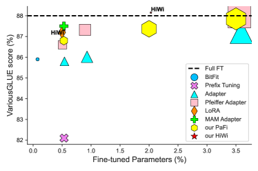
Figure 1: Comparison among various PEFT methods. (Zoom in for a better experience.) Marker size denotes the storage requirement. HiWi stores the least and its storage is invariant to the number of trainable parameters. Specific values are shown in Table 2.

1 Introduction

Pre-trained language models (PLMs) have served as a cornerstone for various natural language processing applications, favoring downstream tasks by offering a robust initialization Peters et al. (2018); Devlin et al. (2019); Liu et al. (2019, 2020); Brown et al. (2020); Liao et al. (2022). Starting with a pre-trained checkpoint, a model can achieve significantly better performance on tasks of interest than the one from scratch. The most historically common way to adapt PLMs to downstream tasks is to update all pre-trained parameters, full fine-tuning. While full fine-tuning produces numerous state-of-the-art results, it is impractical for storage-constrained and communication-frequent cases, like federated learning McMahan et al. (2017), since it requires a full copy of the fine-tuned model for each task. This issue becomes more severe when PLMs are large-scale Brown et al. (2020); Zhang et al. (2022); Hoffmann et al. (2022); Raffel et al. (2020); Scao et al. (2022); Touvron et al. (2023), the number of tasks in interest grows, or data are privately saved on hundreds of servers for federated learning.

An alternative approach popularized by Houlsby et al. (2019) is parameter-efficient fine-tuning (PEFT), where a small number of task-specific parameters is updated and the majority of PLM’s parameters is frozen. In this way, only one general PLM alongside the modified parameters for each task is saved or transferred. Except for saving memory and training cost, PEFT matches the performance of full fine-tuning with only updating less than $1\%$ of the PLM parameters, quickly adapts to new tasks without catastrophic forgetting Pfeiffer et al. (2021) and often exhibits robustness in out-of-distribution evaluation Li and Liang (2021). These compelling advantages have sparked considerable interest in the adoption of PEFT.

PEFT methods can be split into two categories: sparse and infused fine-tuning. Sparse fine-tuning tunes a small subset of existing parameters without introducing new parameters. One typical example is BitFit Zaken et al. (2022), where only the biases are updated. Nonetheless, BitFit is not scalable because of the fixed bias terms. Diff Pruning Guo et al. (2021) and FISH Mask Sung et al. (2021) alleviate this issue by learning and updating task-specific masked parameters with a specified sparsity ratio. However, different masks are learned under different tasks, making these two methods unsuitable for the federated learning setting, where data is rarely i.i.d. across servers.

Infused fine-tuning introduces new parameters to PLMs, and only updates these parameters during training. For example, adapter fine-tuning Houlsby et al. (2019); Pfeiffer et al. (2021) inserts adapters to each layer of the PLM. Other methods, like Prefix Tuning Li and Liang (2021) and Prompt Tuning Lester et al. (2021), append trainable vectors to input or hidden layers. However, inference latency is typically introduced by the newly added parameters and is nonnegligible for some complex tasks, like machine translation (MT) and summarization that add more than $4\%$ of the PLM parameters He et al. (2022).

In this paper, we address the above-mentioned challenges from sparse and infused fine-tuning by proposing two methods, PaFi and HiWi (illustrated in Figure 2). PaFi is a sparse fine-tuning method that selects trainable parameters in a task-agnostic way. I.e., we have the same mask for various downstream tasks. The mask generation of PaFi is also data-less. It doesn’t require any training on any data. HiWi is an infused fine-tuning method that applies the adapters directly to pre-trained weights or biases instead of to hidden representations. After training, the adapters are abandoned, therefore sharing the same inference speed as full fine-tuning.

Our main contributions in this paper are: (1) We introduce two novel transfer learning methods that solve the above-mentioned key challenges of sparse and infused fine-tuning. (2) We empirically evaluate PaFi on the GLUE benchmark and show its effectiveness over existing sparse fine-tuning methods. (3) We compare our methods to a wide range of baselines on a newly constructed benchmark that contains tasks in different types and resources. HiWi outperforms all baselines and full fine-tuning, while requiring the minimum storage (see Figure 1). (4) Our proposed methods still show their effectiveness on a complex task, i.e. machine translation. And all PaFi and HiWi share the same inference speed as full fine-tuning.

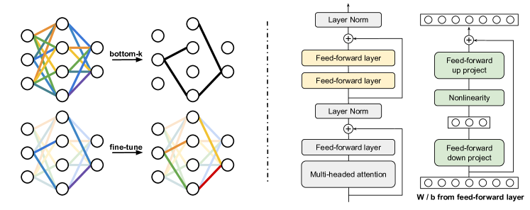
Figure 2: Our proposed methods. PaFi (left): We specify the pre-trained parameters with the smallest absolute magnitude as trainable (upper plot) and only update them during fine-tuning (bottom plot). HiWi (right): Instead of feeding hidden representation to an adapter, we input the pre-trained weights or biases from the feed-forward layers (in yellow) to the adapter and throw the adapter away after training. Only the modules in green are trainable.

2 Preliminaries

In this section, we give an overview of sparse fine-tuning and adapter fine-tuning, and highlight the key challenges of these PEFT methods.

Sparse Fine-Tuning. Sparse fine-tuning formulates a task-specific fine-tuning as a two-phase learning problem. In the first phase, one needs to determine which subset of the pre-trained parameters $\bm{\theta}^{(0)}$ can be modified by generating a sparse mask $\bm{m}\in\{0,1\}^{|\bm{\theta}^{(0)}|}$, where 1s in $\bm{m}$ denote the corresponding parameters are trainable. BitFit Zaken et al. (2022) heuristically specifies the bias terms trainable. Diff Pruning Guo et al. (2021) and LT-SFT Ansell et al. (2022) fully fine-tune PLM on downstream task to obtain $\bm{\theta}^{(1)}$. And the $k$ parameters with the greatest absolute difference $|\bm{\theta}^{(1)}-\bm{\theta}^{(0)}|$ are selected for updating in the next phase. FISH Mask Sung et al. (2021) uses the gradient information of $\bm{\theta}^{(1)}$ to learn the mask.

After obtaining the mask, the PLM is fine-tuned and only the masked parameters are updated whereas the others are frozen. The learning procedure of the second phase is defined as

$$\bm{\theta}^{(2)}=\operatorname*{argmin}_{\bm{\theta}}\mathcal{L}(\mathcal{D};\bm{m}\odot\bm{\theta})$$ (1)

with $\bm{\theta}$ initialized by $\bm{\theta}^{(0)}$, where $\mathcal{L}$ and $\mathcal{D}$ are the objective and data of downstream task, respectively. In addition, $(\bm{1}-\bm{m})\odot\bm{\theta}^{(2)}=(\bm{1}-\bm{m})\odot\bm{\theta}^{(0)}$, since we only update the masked parameters. In the end, only a common $\bm{\theta}^{(0)}$, the updated parameters $\bm{m}\odot\bm{\theta}^{(2)}$ and their indices are saved, which is storage-friendly with a large number of downstream tasks.

Adapter Fine-Tuning. Adapter fine-tuning methods Houlsby et al. (2019); Pfeiffer et al. (2021) insert one or multiple small MLP modules into each layer of the PLM. This MLP module consists of a down ($\bm{W}_{down}\in\mathbb{R}^{d\times r}$) and up ($\bm{W}_{up}\in\mathbb{R}^{r\times d}$) projection pair, where $r$ is the bottleneck dimension, $d$ is the dimension of hidden representation and $r\ll d$. Most adapter fine-tuning methods can be fed into the formula of

$$\bm{h}\leftarrow\bm{h}+f(\bm{h}\bm{W}_{down})\bm{W}_{up}$$ (2)

where $\bm{h}$ is the input to the adapter and $f(\cdot)$ is a nonlinear function.

The adapter fine-tuning methods in the formula of Equation 2 are module-wise, which means they consider the attention module or the feed-forward module as a unit and insert the adapter in between or after these units. In contrast, LoRA Hu et al. (2022) inserts the adapter layer-wise as:

$$\bm{h}\leftarrow\bm{h}\bm{W}+\bm{h}\bm{W}_{down}\bm{W}_{up}$$ (3)

where $\bm{W}\in\mathbb{R}^{d\times d}$ is a pre-trained weight. LoRA has the same inference speed as full fine-tuning, since we can pre-compute $\bm{W}\leftarrow\bm{W}+\bm{W}_{down}\bm{W}_{up}$ and use the new $\bm{W}$ for inference. Both sparse fine-tuning and adapter fine-tuning can be fed into a unified framework.

A Unified Framework for Sparse and Adapter Fine-Tuning. Normally, we initialize $\bm{W}_{down}$ and $\bm{W}_{up}$ (or at least one of them) close to $\bm{0}$ Houlsby et al. (2019); Hu et al. (2022), so the initial state of $\bm{h}$ is close to the original state $\bm{h}$ of PLM, which makes the fine-tuning empirically perform better. This initialization is important for PEFT in case of the catastrophic forgetting of the pre-training knowledge. Supposed we defined the newly added parameters ($\bm{W}_{down}$s and $\bm{W}_{up}$s) for adapter fine-tuning as $\bm{\delta}$, the initialization of $\bm{\delta}$ (i.e. $\bm{\delta}^{(0)}\approx\bm{0}$) fulfills $\mathcal{L}^{pre}(\cdot;\bm{\phi}^{(0)})\approx\mathcal{L}^{pre}(\cdot;\bm{\theta}^{(0)})$, where $\mathcal{L}^{pre}$ is the pre-training objective and $\bm{\phi}^{(0)}=\{\bm{\theta}^{(0)},\bm{\delta}^{(0)}\}$.

Straightforwardly, we can combine the second phase of sparse fine-tuning (Equation 1) and the adapter fine-tuning as:

$$\hat{\bm{\phi}}=\operatorname*{argmin}_{\bm{\phi}}\mathcal{L}(\mathcal{D};\bm{z}\odot\bm{\phi})$$ (4)

with $\bm{\phi}$ initialized by $\bm{\phi}^{(0)}$, where $\bm{z}\in\{0,1\}^{|\bm{\phi}^{(0)}|}$. For sparse fine-tuning, the 1s in $\bm{z}$ only locates for the trainable parameters in $\bm{\theta}^{(0)}$, whereas all locations for $\bm{\delta}^{(0)}$ in $\bm{z}$ are 1s for adapter fine-tuning. In a word, the subset of the trainable parameters in $\bm{\phi}$ is fixed for adapter fine-tuning, but task-specific for sparse fine-tuning.

Key Challenges. Sparse fine-tuning normally gains less attention than adapter fine-tuning. The reasons are two-fold: (1) In the first phase of sparse fine-tuning, the generation of the sparse mask is task-specific, which means different downstream tasks or the same task with different domain data might have different masks, whereas adapter fine-tuning always has fixed positions for adapters; (2) One needs some tricks to generate these masks, like a differential version of $L_{0}$ norm Guo et al. (2021) or Fisher Information Sung et al. (2021), which requires more computation than a normal full fine-tuning for the same iterations.

Compared to sparse fine-tuning, adapter fine-tuning typically introduces additional inference latency from the newly added parameters. Though LoRA doesn’t have this issue, one can’t apply a nonlinear function in the adapter for LoRA since

$$\bm{h}\bm{W}+f(\bm{h}\bm{W}_{down})\bm{W}_{up}$$

$$\neq \bm{h}(\bm{W}+f(\bm{W}_{down})\bm{W}_{up})$$ (5)

, which limits the learning capacity of this method.

3 Methodologies

Motivated by the key challenges stated in Section $\S$2, we propose two methods in this section and illustrate them in Figure 2: one for sparse fine-tuning that generates a universal mask for various tasks without any training, and another one for adapter fine-tuning that has the same inference speed as full fine-tuning while requiring even less storage than BitFit Zaken et al. (2022).

3.1 Task-Agnostic Mask Generation

Compared to adapter fine-tuning with fixed parameters to tune, existing sparse fine-tuning methods typically require extra training to determine which parameters are trainable. This procedure not only requires more computation than full fine-tuning but also hinders the application of this method to federated learning where data is rarely i.i.d. Based on this issue, we propose a research question: could we universally select a set of trainable parameters for different tasks?

To solve this question, we look into the benefit of sequential pre-training and fine-tuning. Aghajanyan et al. (2021) stated that PLM learns generic and distributed enough representations of language to facilitate downstream learning of highly compressed task representation. We hypothesize that the important (in some sense) parameters of a PLM learn a more generic representation of language and therefore favor downstream tasks more than the others. Therefore, we should fix these parameters and only update the unimportant ones. One might argue that the important parameters of a PLM could also be the ones important to downstream tasks and we should train them rather than fix them. We empirically justify our claim in Section $\S$5.5.

Now the question goes to how to select the unimportant parameters so that we can fine-tune them on downstream tasks later. Here we offer two options: one with training on pre-training data and one in a data-less way. Inspired by FISH Mask Sung et al. (2021) where the unimportant parameters are the ones with less Fisher information, we can approximate the Fisher information matrix Fisher (1992); Amari (1996) as

$$\hat{\bm{F_{\theta}}}=\frac{1}{N}\sum_{i=1}^{N}(\triangledown_{\bm{\theta}}\mathcal{L}^{pre}(\mathcal{D}_{i};\bm{\theta}))^{2}$$ (6)

where $\hat{\bm{F_{\theta}}}\in\mathbb{R}^{|\bm{\theta}|}$, $\mathcal{D}_{i}$ is a sample from the pre-training corpus and $\mathcal{L}^{pre}$ is the pre-training objective. An intuitive explanation of Equation 6 is: The parameters with a larger value in $\hat{\bm{F_{\theta}}}$ are more important since they cause larger gradient updates. Then the sparse mask comprises the parameters $\{\bm{\theta}_{i}|\hat{\bm{F}}_{\bm{\theta}_{i}}\leq sort(\hat{\bm{F}}_{\bm{\theta}})_{k}\}$, since we only update the unimportant parameters.

Another method is magnitude-based. We simply consider the pre-trained parameters with the smallest absolute magnitude as the unimportant ones, since they contribute the least to the pre-training loss. Then the sparse mask consists of the parameters $\{\bm{\theta}_{i}||\bm{\theta}_{i}|\leq sort(|\bm{\theta}|)_{k}\}$.

In this paper, we only explore the magnitude-based method and leave another one for future work. The main reason is: The magnitude-based method doesn’t require any training on any data, whereas another method requires the calculation of gradients on pre-training data that are normally large-scale and private for some PLMs. We name our method as PaFi, since it follows a procedure of Pruning-and-Finetuning.

3.2 Adapter for Pre-trained Parameters

Compared to sparse fine-tuning that tunes a small portion of existing parameters, adapter fine-tuning introduces new parameters at some fixed positions for different tasks. Normally, the number of added parameters correlates with the complexity of the downstream task. For example, one can add 0.5% of the PLM parameters to achieve the same performance as full fine-tuning for the GLUE benchmark, while 4% is required for machine translation He et al. (2022). The inference speed of a task is proportional to the number of added parameters, so the introduced inference latency is nonnegligible for complex tasks.

Inspired by LoRA Hu et al. (2022) which has the same inference speed as full fine-tuning, we propose a new adapter fine-tuning method that applies an adapter directly to pre-trained parameters instead of hidden representations as:

$$\bm{W}\leftarrow\bm{W}+f(\bm{W}\bm{W}_{down})\bm{W}_{up}$$ (7)

If we neglect the nonlinear function, a representation $\bm{h}$ through our linear layer becomes $\bm{hW}(\bm{1}+\bm{W}_{down}\bm{W}_{up})$. Compared to LoRA (See Equation 3) where the learned diff matrix is $\triangle\bm{W}=\bm{W}_{down}\bm{W}_{up}$, our learned diff matrix is $\triangle\bm{W}=\bm{W}\bm{W}_{down}\bm{W}_{up}$. Without considering the nonlinear function, the rank of the diff matrix from LoRA is the upper bound of the rank for our diff matrix:

$$rank(\bm{WW}_{down}\bm{W}_{up})$$

$$\leq min(rank(\bm{W}),rank(\bm{W}_{down}\bm{W}_{up}))$$

$$= rank(\bm{W}_{down}\bm{W}_{up})$$ (8)

The equality holds since the rank of a pre-trained weight is empirically larger. To improve the learning capacity (it is related to the matrix rank) of our method, we input a nonlinear function between $\bm{W}_{down}$ and $\bm{W}_{up}$, which is not possible for LoRA if we want to maintain the same inference speed as full fine-tuning (see Equation 5).

One obvious advantage of our method is that it has the same inference speed as full fine-tuning, since we can compute $\bm{W}\leftarrow\bm{W}+f(\bm{W}\bm{W}_{down})\bm{W}_{up}$ before the inference step. Another advantage is: we can replace the weight matrix in Equation 7 with the bias term. I.e. we input the pre-trained bias to an adapter to construct a new bias. In this way, we can solve the issue raised by BitFit Zaken et al. (2022), where the number of bias terms is fixed and therefore BitFit is not scalable. When we apply the adapter to the weight matrix, we need to save $\bm{W}_{down}$ and $\bm{W}_{up}$, since their size are much smaller than $\bm{W}$. However, when we apply the adapter to bias terms, we only need to save the new bias ($\bm{b}\leftarrow\bm{b}+f(\bm{b}\bm{W}_{down})\bm{W}_{up}$) that requires much less storage than saving $\bm{W}_{down}$ and $\bm{W}_{up}$. It also means we require the same storage (for the bias terms) whatever the size of $\bm{W}_{down}$ and $\bm{W}_{up}$, and therefore we can use a large number of trainable parameters. We name our method as HiWi, since it Hides (throws away) the Weights from adapters.

4 Experimental Setup

4.1 Evaluation Tasks

Due to limited computation resources, we select six tasks from the GLUE Wang et al. (2019b) and SuperGLUE Wang et al. (2019a) benchmarks: two natural language inference tasks (MNLI and RTE), a similarity task (STS-B), a word sense disambiguation task (WiC), a coreference resolution task (WSC) and a causal reasoning task (COPA). For most tasks, we follow the RoBERTa paper Liu et al. (2019), treating MNLI and RTE as sentence-level classification tasks, WiC as a word-level classification task, STS-B as a regression task and WSC as a ranking task. Nevertheless, we implement COPA as a ranking classification task rather than a binary classification task in Liu et al. (2019), since it offers better performance for all methods.

We term our selected tasks VariousGLUE, since they cover a wide range of tasks (classification, ranking, regression) and include high-resource (MNLI), middle-resource (STS-B, WiC and RTE) and low-resource (WSC, COPA) tasks. For evaluation on VariousGLUE, we report accuracy for MNLI, WiC, RTE, WSC and COPA, and the Pearson correlation coefficient for STS-B on the development sets. More data statistics, implementation details and task selection criteria of VariousGLUE are in Appendix $\S$A. Except for natural language understanding (NLU) tasks, we also evaluate our methods on a sequence-to-sequence task, i.e. English to Romanian translation with the WMT 2016 En-Ro dataset Bojar et al. (2016), and report BLEU Papineni et al. (2002) on the test set.

Method	#Tuned	MNLI	QQP	QNLI	SST-2	CoLA	STS-B	MRPC	RTE	Avg
Full FT Liu et al. (2019)	100%	90.2	92.2	94.7	96.4	68.0	92.4	90.9	86.6	88.9
Our Full FT	100%	90.10.09	92.30.00	94.80.05	96.40.21	69.00.82	91.90.17	91.70.14	88.10.63	89.30.26
Linear FT	0%	52.40.47	75.60.19	67.40.05	83.70.25	00.00.00	31.23.50	69.90.19	54.50.14	55.10.60
Linear FTnorm	0.03%	88.40.00	87.80.05	92.50.12	95.10.05	47.00.79	75.31.89	71.10.14	53.40.79	76.30.48
Adapter†	0.2%	90.30.3	91.50.1	94.70.2	96.30.5	66.32.0	91.50.5	87.71.7	72.92.9	86.41.0
Adapter†	1.7%	89.90.5	92.10.1	94.70.2	96.20.3	66.54.4	91.01.7	88.72.9	83.41.1	87.81.4
Pfeiffer Adapter†	0.2%	90.50.3	91.70.2	94.80.3	96.60.2	67.82.5	91.90.4	89.71.2	80.12.9	87.91.0
Pfeiffer Adapter†	0.8%	90.20.3	91.90.1	94.80.2	96.10.3	68.31.0	92.10.7	90.20.7	83.82.9	88.40.8
LoRA Hu et al. (2022)	0.2%	90.60.2	91.60.2	94.80.3	96.20.5	68.21.9	92.30.5	90.21.0	85.21.1	88.60.7
Diff Pruning	0.5%	90.30.08	90.30.17	94.60.22	96.40.21	65.12.39	92.00.17	90.21.11	84.51.18	87.90.69
FISH Mask	0.5%	90.20.08	89.80.17	94.10.26	96.10.38	66.31.89	92.50.08	88.70.92	86.31.07	88.00.61
PaFi	0.5%	90.20.05	90.30.05	94.60.08	96.70.19	70.20.46	91.90.24	91.40.14	88.80.63	89.30.23

Table 1: Sparse fine-tuning on GLUE. The best and second-best scores are in bold and underlined, respectively. Results of methods with “†” are also copied from Hu et al. (2022). The tasks are ordered with their number of samples from largest to smallest.

4.2 Baselines

To compare with other baselines broadly, we replicate their setups since most of them are not evaluated on the same tasks or use the same PLM (RoBERTa_LARGE) as ours. If possible, we also report their scores.

Full fine-tuning (Full FT) updates all parameters. Linear fine-tuning (Linear FT) only tunes the added classifier. Linear fine-tuning with normalization (Linear FT_norm) fine-tunes the classifier and all normalization layers of the PLM. We borrow the fine-tuning recipe from Liu et al. (2019) for these three baselines.

Both Diff Pruning Guo et al. (2021) and FISH Mask Sung et al. (2021) are chosen as sparse fine-tuning baselines. We implement them on their own frameworks with their own recipes (combined with our recipe for middle-/low-resource tasks).

We select three adapter variants as our baselines: Adapter Houlsby et al. (2019), Pfeiffer Adapter Pfeiffer et al. (2021) and LoRA Hu et al. (2022). In addition, we also compare our methods to BitFit Zaken et al. (2022), Prefix Tuning Li and Liang (2021) and MAM Adapter He et al. (2022). MAM Adapter combines prefix tuning and adapter, offering a new state-of-the-art.

If not specified otherwise, we reproduce these baselines on RoBERTa_LARGE with our own training recipe (see Section $\S$4.3), if they don’t offer results on our selected tasks or use different PLMs. You can find more details about the calculation of trainable parameters and storage requirements of these methods in Appendix $\S$B.

4.3 Implementation

We use the encoder-only RoBERTa_LARGE model Liu et al. (2019) as the underlying model for all NLU tasks and the encoder-decoder mBART_LARGE model Liu et al. (2020) for MT. All our implementations are on the Fairseq framework Ott et al. (2019). For NLU tasks, we sweep learning rates in {3, 4, 5, 6, 7} $\cdot 10^{-4}$ (inspired by the best results obtained in LoRA Hu et al. (2022)), batch sizes in {16, 32}, and the number of epochs in {10, 20} (for tasks with the number of samples over 100K, we only train for 10 epochs). Other settings of the optimizer stay the same as the RoBERTa paper. For the En-Ro task, we borrow the same training recipe from He et al. (2022), i.e. setting the learning rate as $5\cdot 10^{-5}$, a mini-batch with 16384 tokens, a label smoothing factor of 0.1 Szegedy et al. (2016); Gao et al. (2020) for 50K iterations.

We run all experiments on a single NVIDIA RTX A6000 GPU with 48G memory. In addition, we run the same task of a method in the above-mentioned grid search space three times with different random seeds, choose the best result from each run, and report the median and standard deviation of these three best results.

PaFi and HiWi. By default, we select the bottom-k parameters for PaFi group-wise rather than globally. I.e. we select $k$ parameters with the smallest absolute magnitude within each group (a weight matrix or a bias term is considered as a group) and only fine-tune them. In addition, we fine-tune all parameters from normalization layers and don’t update the token and position embeddings at all. More discussion about this setting is in Section $\S$5.5. For HiWi, the default setting is feeding the bias rather than the weight to an adapter, because it requires much less storage.

Method	#Tuned	#Stored	MNLI	WiC	STS-B	RTE	WSC	COPA	Avg
Full FT†	100%	100%	90.2	75.6	92.4	86.6	-	94.0	-
Our Full FT	100%	100%	90.10.09	74.00.41	91.90.17	88.10.63	87.51.09	96.00.47	88.00.48
Linear FT	0%	0%	52.40.47	67.60.46	31.23.50	54.50.14	68.30.00	72.01.63	58.71.04
Linear FTnorm	0.03%	0.03%	88.41.42	67.90.33	75.31.89	53.40.79	75.90.85	74.01.41	73.00.88
BitFit	0.08%	0.08%	89.50.05	71.90.45	91.40.09	88.10.33	85.71.53	89.01.24	85.90.62
Prefix Tuning	0.5%	0.5%	89.90.12	69.70.62	91.40.75	76.52.1	91.11.59	74.01.89	82.11.18
Adapter	0.5%	0.5%	90.60.16	71.90.12	92.10.21	87.40.45	84.81.00	88.02.16	85.80.69
Pfeiffer Adapter	0.5%	0.5%	90.80.08	71.90.47	92.10.26	88.40.46	86.70.40	90.00.94	86.60.44
LoRA	0.5%	0.5%	90.60.17	72.30.68	91.70.24	88.41.02	88.40.42	92.02.36	87.20.81
MAM Adapter	0.5%	0.5%	90.60.17	72.40.79	92.10.05	89.51.09	88.30.05	92.00.47	87.50.44
PaFi	0.5%	0.5%	90.20.05	72.60.14	91.90.24	88.80.63	85.20.45	92.01.70	86.80.54
HiWi (r=4)	0.5%	0.03%	90.20.05	73.40.83	91.60.05	88.10.05	87.50.42	93.00.00	87.30.23
HiWi (r=16)	2.0%	0.03%	90.20.09	73.70.33	91.90.17	88.80.33	89.32.25	95.01.25	88.20.74

Table 2: Results on VariousGLUE. The tasks are ordered with their number of samples from largest to smallest. The best and second-best scores are in bold and underlined, respectively. Results of the method with “†” are copied from Liu et al. (2019). Notably, the storage of HiWi is invariant to the number of trainable parameters.

Method	#Tuned	#Stored	BLEU
Full FT†	100%	100%	37.3
BitFit†	0.05%	0.05%	26.4
Prefix Tuning†	10.2%	2.4%	35.6
Pfeiffer Adapter†	4.8%	4.8%	36.9.1
LoRA(ffn)†	4.1%	4.1%	36.8.3
MAM Adapter†	14.2%	4.5%	37.5.1
PaFi	4.5%	4.5%	37.7.1
PaFi	14.2%	14.2%	38.3.1
HiWi for Bias	4.7%	0.02%	28.0.2
HiWi for Weight	4.7%	4.7%	36.9.2

Table 3: Results on WMT 2016 En-Ro. The best and second-best scores are in bold and underlined, respectively. Results of the methods with “†” are copied from He et al. (2022). $r=64$ for HiWi.

5 Result and Discussion

In this section, we present the results of baselines and our proposed methods on GLUE, VariousGLUE and translation tasks.

5.1 Sparse Fine-Tuning on GLUE

Since the frameworks of Diff Pruning and FISH Mask only support the GLUE benchmark, we evaluate our proposed sparse fine-tuning method, PaFi, on GLUE and show the results in Table 1, where we follow the sparsity setting of Diff Pruning and FISH Mask, and set it as 0.5%. In the RoBERTa paper Liu et al. (2019), some low-resource tasks (RTE, MRPC and STS-B) are initialized from the fine-tuned model on MNLI rather than the PLM. We don’t follow this setup and always consider the PLM as an initialization as Houlsby et al. (2019). Surprisingly, our reproduction outperforms the reported score in the RoBERTa paper by 0.4%.

Compared to existing sparse and adapter fine-tuning methods, our PaFi obtains the best result, achieving the same score (89.3) as Full FT with only updating 0.5% parameters. PaFi also outperforms Diff Pruning and FISH Mask by a significant margin, with at least a 1.3% improvement on average, which demonstrates the effectiveness of our simple parameter selection method.

In addition, PaFi also shows its efficiency in terms of storage and training compared to other sparse fine-tuning methods. The saving of the indices for updated parameters consumes the same memory as the saving of these parameters if both are in fp32. One only needs to save one mask for PaFi, but the same number of masks as the number of tasks for Diff Pruning and FISH Mask. Our one-mask-for-all setting is also suitable for federated learning, where non-i.i.d. data could use the same mask, which is impossible for Diff Pruning and FISH Mask. For training costs, PaFi doesn’t require any training in the mask generation phase, while Diff Pruning and FISH Mask require more computation ($>2$ times for Diff Pruning) than Full FT because of the calculation of differential $L_{0}$ norm or Fisher information matrix. Specifically on the MNLI task, Diff Pruning, FISH Mask and PaFi spend 19.9h, 1m39s and 2s to generate the sparse mask, respectively. And both Diff Pruning and FISH Mask require the data of downstream task for the mask generation, while the mask generation of PaFi is data-less.

5.2 Results on VariousGLUE

Table 2 shows the results of different methods on VariousGLUE. For most methods, the number of trainable parameters stays the same as the number of stored parameters. However, Prefix Tuning and MAM Adapter apply a re-parameterization trick and throw away some trainable parameters after training, which might result in different numbers (see Appendix $\S$B). In addition, the storage requirement of HiWi is invariant to the number of trainable parameters since we throw away all adapter parameters and only save the new bias terms.

Compared to Table 1, PaFi performs unexpectedly worse, which justifies the necessity of evaluation on various tasks for PEFT methods. On high-resource (MNLI) and most middle-resource (STS-B and RTE) tasks, PaFi is on par with Full FT. Though not the best, PaFi still outperforms some adapter fine-tuning methods (Adapter and Pfeiffer Adapter), which shows tuning existing parameters is enough for some tasks.

When using the same number of trainable parameters (0.5%), HiWi performs on par with the best baseline, MAM Adapter (87.3 vs 87.5). Notably, MAM Adapter is an additive work that combines Prefix Tuning and adapters together. We could also implement HiWi and Prefix Tuning in the same framework and leave this exploration to future work. If we increase the number of trainable parameters to 2% (almost requiring the same training time and memory footprint as 0.5%), HiWi outperforms all baselines and Full FT (88.2 vs 88.0). Notably, HiWi only requires a fixed storage, around 0.03% of the PLM total parameters, which is also the least storage requirement among all methods.

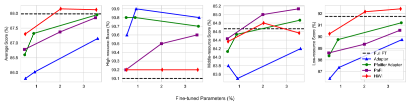
Figure 3: Scalability of different methods: (a) Average performance on VariousGLUE. (b)(c)(d): average performance on high-resource (MNLI), middle-resource (WiC, STS-B, RTE) and low-resource (WSC, COPA) tasks.

Method	WiC	RTE	COPA
Full FT	74.00.41	88.10.63	96.00.47
Smallest	72.60.14	88.80.63	92.01.70
Largest	72.90.54	84.10.66	90.00.81
Middle	72.70.45	83.80.85	90.00.82
Random	71.90.40	84.51.80	91.00.94
Not tune norm	72.40.57	88.10.45	90.00.94
Tune embed	72.60.24	88.40.14	91.00.94

Table 4: Ablation studies of PaFi on: (1) How to choose trainable parameters; (2) Which groups should be tuned. The method in gray is PaFi with the default setting.

5.3 Results on MT

Compared to NLU tasks, where the number of trainable parameters is negligible, MT task requires more trainable parameters to achieve a similar result as Full FT. We show the results of different methods on WMT 2016 En-Ro in Table 3. PaFi performs the best and outperforms Full FT (37.7 vs 37.3 with 4.5% parameters). Similar to the conclusion that we draw from Table 2, PaFi is good at high- and middle-resource tasks.

HiWi for bias works unexpectedly worse, while HiWi for weight is on par with LoRA. We argue: Though we can improve the learning capacity of bias terms with adapters, the limited amount of biases still hinders HiWi’s representative ability. HiWi for weight solves this issue by feeding a much larger amount of weights to adapters. In addition, most baselines, except for BitFit and LoRA, introduce nonnegligible inference latency (proportional to the stored parameters), while PaFi and HiWi share the same inference speed as Full FT. Specifically, the inference time on En-Ro is 110s for Full FT, LoRA, HiWi and PaFi, while it’s 125s for Pfeiffer Adapter (13.6% more inference latency).

5.4 Scalability

Not all PEFT methods benefit monotonically from having more trainable parameters. Li and Liang (2021) and Hu et al. (2022) have shown that Prefix Tuning can’t be scaled up well. Here we investigate the scalability of our methods and show the results in Figure 3. On average, all listed methods could be scaled well, and HiWi always outperforms other methods. However, these methods show different scaling behaviors for tasks in different resources.

For the high-resource task, HiWi performs the worst and is stable with an increasing number of trainable parameters, while PaFi shows a well-behaved pattern. This also explains the best performance of PaFi on En-Ro. I.e. PaFi could obtain stronger performance for the setting of a high-resource task and a high number of trainable parameters. For middle-resource tasks, PaFi outperforms other methods and still has a good scaling behavior. For low-resource tasks, HiWi performs the best. The best overall performance of HiWi mainly benefits from these low-resource tasks, which shows HiWi is an effective option for the low-resource or few-shot learning setting.

In summary, PaFi shows its superiority when the task is high-resource and the number of tunable parameters is not too small, while the superiority of HiWi locates in the low-resource (for tasks and the number of tunable parameters) setting.

5.5 The Default Setting of PaFi

Table 4 shows our investigation of the PaFi’s settings. We implement four ablation experiments on how to choose the trainable parameters. Overall, updating the parameters with the smallest absolute magnitudes offers the best results. The gap between our default setting and other options is the largest for RTE. In addition, tuning the normalization layers is necessary for all tasks.

The results of tuning embeddings are similar to the results of without tuning embeddings, but a little lower. According to Figure 4 (in Appendix), the embedding layer always has a higher mean, twice as the mean from other layers. This is also one reason why we don’t tune parameters from the embedding layer, since most of them have a higher absolute magnitude, showing that they are important. Another reason is that the embedding layer occupies a large number of parameters. We can spare the budget for trainable parameters from this layer and share it with other layers.

6 Related Works

Parameter-Efficient Fine-Tuning for PLMs. Sparse fine-tuning Zaken et al. (2022); Guo et al. (2021); Sung et al. (2021) offers a tool to explore the over-parameterization of PLMs and doesn’t introduce additional latency. Infused fine-tuning Houlsby et al. (2019); Pfeiffer et al. (2021); Hu et al. (2022); He et al. (2022) is highly modularized and has a lower task-switching overhead during inference. Our PaFi simplifies existing sparse fine-tuning methods and makes it more practical for the communication-frequent setting (federated learning). Our HiWi lowers the requirement for storage to a scale and doesn’t induce any inference latency.

Other efficient parameterization methods, like COMPACTER Mahabadi et al. (2021), efficiently parametrize the adapter layers and reduce the number of trainable parameters. They are orthogonal to our work and can be combined with our HiWi. A recently proposed activation method, (IA)³ Liu et al. (2022), achieves a new state-of-the-art on few-short learning and has a similar storage requirement as HiWi. However, it can’t be scaled up and performs worse than adapter fine-tuning methods when the number of samples is not too small.

Pruning. Network pruning is a technique for sparsifying neural networks while sacrificing minimal performance Theis et al. (2018); Liu et al. (2021). Though we borrow some methods from it, like parameter selection with magnitude or Fisher information, we don’t prune any parameter and maintain a similar performance as full fine-tuning.

7 Conclusion

In this work, we first propose PaFi as a novel but simple method for computing the sparse mask without any training and in a task-agnostic way. It selects the parameters with the lowest absolute magnitude from PLMs and tunes them, with keeping others frozen. We demonstrate the effectiveness of PaFi on the GLUE benchmark and translation task. Secondly, we propose HiWi as an adapter fine-tuning method that feeds pre-trained parameters instead of hidden representations to the adapters. It doesn’t introduce any inference latency. Furthermore, it requires the lowest storage while outperforming other strong baselines. In the future, we will try to compute the sparse mask with Fisher information and estimate our methods in a realistic few-shot learning setting.

Limitations

We acknowledge the main limitation of this work is that we only evaluate our methods on some tasks from the GLUE and SuperGLUE benchmarks due to limited computation resources. And all tasks are not in a realistic few-shot setting, where the number of training samples is less than a few hundred and development sets are not offered. The benefit of PEFT methods could come from an exhaustive search of hyper-parameters for the development sets, while the realistic few-shot setting could solve this issue and shed more light on PEFT. It would be interesting to see how our methods and other baselines perform on a wide range of few-shot tasks.

In addition, current frameworks are not friendly for sparse fine-tuning methods. Most works (Diff Pruning, FISH Mask and our PaFi) still need to calculate a full gradient of all parameters and selectively update the masked parameters, which makes it cost the same training time as full fine-tuning.

Last but not least, we only estimate our methods on one single complex task, i.e. WMT 2016 En-Ro. One might not draw the same conclusion as ours on other complex tasks, like machine translation for different languages and resources, summarization tasks, and so on.

Ethics Statement

The PLMs involved in this paper are RoBERTa_LARGE and mBART_LARGE. RoBERTa_LARGE was pre-trained on BookCorpus Zhu et al. (2015), CC-News Nagel (2016), OpenWebText Gokaslan and Cohen (2019) and Stories Trinh and Le (2018). mBART_LARGE was pre-trained on CC25 extracted from Common Crawl Wenzek et al. (2020); Conneau et al. (2020). All our models may inherit biases from these corpora.

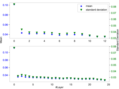
Figure 4: Mean and standard deviation of parameters’ absolute magnitudes from different layers. Up: RoBERTa_BASE, Bottom: RoBERTa_LARGE. The 0^th layer denotes the token and position embeddings.

Appendix A Experimental Detail

A.1 Data Statistics

We show the statistics of VariousGLUE and En-Ro in Table 5. We test our methods on four types of tasks that are high-resource (MNLI and En-Ro), middle-resource (STS-B, WiC and RTE) or low-resource (WSC and COPA).

A.2 Implementation Details of VariousGLUE

Due to limited computation resources, we could not evaluate our methods and baselines on all tasks from the GLUE Wang et al. (2019b) and SuperGLUE Wang et al. (2019a) benchmarks. We select six tasks from these two benchmarks. Except for COPA, we follow the same implementation as RoBERTa Liu et al. (2019). We list the details as follows:

• MNLI Williams et al. (2018) and RTE Dagan et al. (2005); Bar-Haim et al. (2006); Giampiccolo et al. (2007); Bentivogli et al. (2009): The input format is “[CLS] sentence₁ [SEP] [SEP] sentence₂ [SEP]”. We input the representation of the [CLS] token from the encoder to a multi-class classifier for prediction.

• WiC Pilehvar and Camacho-Collados (2019): WiC has the same input format as MNLI and RTE. We feed the concatenation of the representation of the two marked words and the [CLS] token to a binary classifier.

• STS-B Cer et al. (2017): STS-B also has the same input format as MNLI and RTE. We feed the representation of the [CLS] token to a regression layer (similar to the classification layer with only one class).

• WSC Levesque et al. (2012): We first detect all noun phrases from the sentence. Supposed $n$ noun phrases are detected, we replace the pronoun with these phrases to construct $n$ new sentences and input them to RoBERTa in a batch way in the format of “[CLS] sentence [SEP]”. After the masked word prediction layer, we take the corresponding logits for these $n$ noun phrases. Some noun phrases might be a span. We average the logits in this span to obtain a single logit for each noun phrase. For the sample that offers a correct match between the noun phrase and the pronoun, we assign 1 as a label to the logit of this noun phrase and 0 to the other and calculate the cross-entropy loss. Even though we have to throw away the annotated samples that have incorrect matches, this method offers the best result. During inference, the noun phrase with the biggest logit is the prediction.

• COPA Roemmele et al. (2011) The input format for a single sample is “[CLS] Because sentence₁, so sentence₂ [SEP]” or “[CLS] Because sentence₂, so sentence₁ [SEP]”. We feed these two inputs from the same sample to RoBERTa in a batch way, then input the representation of both [CLS]s to a classifier with only one class, making sure the logit from the input with the correct causal effect is larger than another one by calculating the cross-entropy loss.

Except for WSC, we always insert a classifier layer on top of the RoBERTa encoder. For WSC, we use the original masked word prediction layer from the PLM and keep it frozen. You can find more implementation details in our codebase.

Type	Name	#Train	#Dev.
classification	MNLI	392702	19647
	WiC	5428	638
	RTE	2490	277
regression	STS-B	5749	1500
ranking	WSC	554	104
	COPA	400	100
translation	En-Ro	610320	1999

Table 5: Statistics of evaluation tasks. The test set of En-Ro also has 1999 samples.

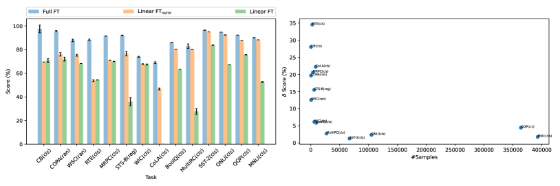
Figure 5: Task Selection. Left: The performance of the tasks from the GLUE and SuperGLUE benchmarks for different methods. The tasks are ordered with their number of samples from smallest to largest. The short terms in the brackets denote the task type. “cls”, “ran” and “reg” are the short terms of classification, ranking and regression, respectively. Right: Performance difference between Linear FT_norm and Full FT.

Full FT	Linear FTnorm	Linear FT
88.50.67	75.80.47	57.80.78

Table 6: The average performance on all tasks.

A.3 Criteria for Task Selection

Most PEFT methods are evaluated on the GLUE benchmark. We argue that the GLUE tasks might be too easy for PLMs, since all GLUE tasks, except for STS-B, are classification tasks and some PLMs outperform our humans by a large margin according to the GLUE leaderboard. In addition, the number of training samples for each GLUE task is big (RTE is the task with the minimum number of samples, 2.5K). Most works have to construct few-shot learning tasks from GLUE by themselves. Compared to GLUE, the SuperGLUE benchmark offers more low-resource tasks and is much more difficult for PLMs. Due to computational resource limits, we can’t evaluate on all GLUE and SuperGLUE tasks, and therefore want to select some tasks from these two benchmarks.

Our selection criteria are three-dimensional: complexity, variety in task type and variety in task resource. Deciding whether a task is easy or complex could be subjective. Since our main research topic in this paper is PEFT, we determine the complexity of a task with its performance improvement from Linear FT_norm to Full FT (see Section $\S$4.2 for these baselines). Linear FT_norm requires the minimum trainable parameters among all PEFT methods. If a task obtains a huge improvement from Linear FT_norm to Full FT, it means this task needs many parameters to tune, and therefore it is difficult for PEFT methods and a complex task.

Figure 5 shows the performance of Full FT, Linear FT and Linear FT_norm on the tasks from GLUE and SuperGLUE. Overall, Linear FT_norm outperforms Linear FT by a large margin, 75.8 vs. 57.8 on average (see Table 6). It means that only tuning the normalization layers is an efficient method. With an increasing number of samples, the gap between Full FT and Linear FT_norm normally becomes narrower, which shows the fine-tuning of high-resource tasks requires less trainable parameters than low-resource.

From the perspective of task variety, we want to make sure all task types appear in our VariousGLUE. COPA, WSC, STS-B and WiC are chosen because of their uniqueness. They are sentence-level ranking, word-level ranking, regression and word-level classification tasks, respectively. The rest are all sentence-level classification tasks. From the perspective of complexity and variety in resources, we choose MNLI and RTE, since MNLI has the biggest number of samples and RTE is the most complex and a low-resource task (see right subplot of Figure 5).

Method	#Tuned	#Stored
Full FT	$(V+2+n)d+(12d^{2}+13d)L$	$(V+2+n)d+(12d^{2}+13d)L$
Linear FTnorm	$2d+4dL$	$2d+4dL$
BitFit	$d+11dL$	$d+11dL$
Adapter	$(4dr+2r+6d)L$	$(4dr+2r+6d)L$
Pfeiffer Adapter	$(2dr+r+d)L$	$(2dr+r+d)L$
LoRA	$4drL$	$4drL$
Prefix Tuning	$ld+dm+m+(2md+2d)L$	$2ldL$
MAM Adapter	$ld+dm+m+(2dr+r+3d+2md)L$	$(2dr+r+d+2ld)L$
HiWi for Bias	$(18dr+3r+5d)L$	$5dL$
HiWi for Weight	$(18dr+3r+5d)L$	$(18dr+3r+5d)L$

Table 7: The calculation of trainable and stored parameters. The methods with different calculations for training and storage are highlighted. $V$: the vocabulary size. $n$: the maximum sequence length. $d$: the hidden dimension. $L$: the number of layers. $r$: the bottleneck dimension of the adapter. $m$: the bottleneck dimension of the adapter for Prefix Tuning. $l$: the length of the prefix vector.

Method	Hyper-parameter	#Tuned	#Stored
Adapter (Table 2)	$r=18$	0.5%	0.5%
Adapter (Figure 1 and 3)	$r=32$	0.9%	0.9%
Adapter (Figure 1 and 3)	$r=128$	3.6%	3.6%
Pfeiffer Adapter (Table 2)	$r=36$	0.5%	0.5%
Pfeiffer Adapter (Figure 1 and 3)	$r=64$	0.9%	0.9%
Pfeiffer Adapter (Figure 1 and 3)	$r=128$	3.6%	3.6%
LoRA (Table 2)	$r=18$, $s=2$	0.5%	0.5%
Prefix Tuning (Table 2)	$l=36$, $m=36$	0.5%	0.5%
MAM Adapter (Table 2)	$l=18$, $m=18$, $r=18$, $s=2$	0.5%	0.5%

Table 8: The hyper-parameter values for baselines. $s$ is the scale value for the residual connection.

Appendix B Number of Trainable Parameters and Storage

We summarize the calculation for the number of trainable parameters and storage requirements in Table 7. We only show the calculation of the encoder-only model here. Notably, the newly added classifier for some tasks is excluded from the calculation, since all methods have this same setting. We also show the hyper-parameter values for all baselines used in this paper in Table 8.

Full FT: The number of parameters for the token and position embeddings is $Vd+2d+nd$, where $V$ is the vocabulary size, $d$ is the hidden dimension and $n$ is the maximum sequence length. $2d$ here means the number of parameters from the normalization layer since RoBERTa applies a layer normalization after the embedding. For each encoder layer, RoBERTa has four projection layers for key, value, query and output ($4d^{2}+4d$, $4d$ is the number of parameters for bias), and two feed-forward layers. The first feed-forward layer projects the representation from $d$ to $4d$. And the second one projects it back to $d$. So the number of parameters for these two feed-forward layers is $8d^{2}+5d$ ($5d=4d+d$ for the bias terms). Each layer also has two normalization layers, including $2\times 2d$ parameters. Overall, the size of trainable parameters for Full FT is $(V+2+n)d+(12d^{2}+13d)L$, where $L$ is the number of encoder layers.

Linear FT_norm: Since we only tune the parameters from the normalization layers, so the number of trainable parameters is $2d+4dL$.

BitFit: We tune all bias terms from the normalization layers and the linear layers, so the size is $d+11dL$.

Adapter: We insert two adapter layers to each encoder layer and also tune the normalization layers in the encoder layer, so the size of trainable parameters is $(2(dr+r+rd+d)+4d)L=(4dr+2r+6d)L$, where $r$ is the bottleneck dimension of the adapter.

Pfeiffer Adapter: Pfeiffer Adapter inserts a single adapter to each encoder layer and doesn’t tune the normalization layers, so the size is $(dr+r+rd+d)L=(2dr+r+d)L$.

LoRA: LoRA applies two adapters in parallel to the projection layers for query and value, respectively. Then the number of trainable parameters is $2(dr+rd)L=4drL$ (no bias terms for the adapter).

Prefix Tuning: Prefix Tuning applies a re-parameterization trick to expand the number of trainable parameters. Firstly, it defines an embedding in the size of $l\times d$, where $l$ is the length of the prefix vectors. Then this embedding is fed into a large adapter from $d$ to $2dL$. After the adapter, the embedding is in the size of $l\times 2dL$. We then reshape this matrix to $L\times 2\times ld$, with one prefix vector in the size of $ld$ for the key and another one for the value for each layer. So the number of trainable parameters is $ld+dm+m+2mdL+2dL=ld+dm+m+(2md+2d)L$, where $m$ is the bottleneck dimension for the adapter. However, it is not necessary for us to save all these parameters. We can compute the prefix vectors after training and throw away the embedding and adapter, so the size of stored parameters is $2ldL$.

MAM Adapter: MAM adapter applies Prefix Tuning to the attention module and an adapter in parallel to the MLP module. The number of trainable parameters is the same as the sum of the one for Pfeiffer Adapter and the one for Prefix Tuning, which is $ld+dm+m+(2dr+r+3d+2md)L$. Similar to Prefix Tuning, we can throw away the embedding and adapter for Prefix Tuning after training. So the stored size is $(2dr+r+d+2ld)L$.

HiWi for Bias: HiWi applies one adapter to the bias term (in the size of $4d$) of the first feed-forward layer and another adapter to the bias term (in the size of $d$) of the second feed-forward layer. To avoid allocating too many trainable parameters to the first adapter, we set the bottleneck dimension for the first adapter as $2r$, and the one for the second adapter as $r$. So the size of trainable parameters is $((8dr+2r+8dr+4d)+(dr+r+dr+d))L=(18dr+3r+5d)L$. After training, we compute the new bias and throw away all adapter parameters. So the stored size is $5dL$.

HiWi for Weight HiWi applies one adapter to the weight (in the size of $4d\times d$) of the first feed-forward layer and another adapter to the weight (in the size of $d\times 4d$) of the second feed-forward layer. We only need to swap the order of the above adapters for the bias terms. So the number of trainable parameters stays the same as above, i.e. $(18dr+3r+5d)L$. However, we don’t compute the new weight and throw away the adapters for this case, since the size of the weight matrix is larger than the adapter size. So the stored size is still$(18dr+3r+5d)L$.

References

- Aghajanyan et al. (2021) Armen Aghajanyan, Sonal Gupta, and Luke Zettlemoyer. 2021. Intrinsic dimensionality explains the effectiveness of language model fine-tuning. In Proceedings of the 59th Annual Meeting of the Association for Computational Linguistics and the 11th International Joint Conference on Natural Language Processing, ACL/IJCNLP 2021, (Volume 1: Long Papers), Virtual Event, August 1-6, 2021, pages 7319–7328. Association for Computational Linguistics.
- Amari (1996) Shun-ichi Amari. 1996. Neural learning in structured parameter spaces - natural riemannian gradient. In Advances in Neural Information Processing Systems 9, NIPS, Denver, CO, USA, December 2-5, 1996, pages 127–133. MIT Press.
- Ansell et al. (2022) Alan Ansell, Edoardo Maria Ponti, Anna Korhonen, and Ivan Vulic. 2022. Composable sparse fine-tuning for cross-lingual transfer. In Proceedings of the 60th Annual Meeting of the Association for Computational Linguistics (Volume 1: Long Papers), ACL 2022, Dublin, Ireland, May 22-27, 2022, pages 1778–1796. Association for Computational Linguistics.
- Bar-Haim et al. (2006) Roy Bar-Haim, Ido Dagan, Bill Dolan, Lisa Ferro, and Danilo Giampiccolo. 2006. The second pascal recognising textual entailment challenge. Proceedings of the Second PASCAL Challenges Workshop on Recognising Textual Entailment.
- Bentivogli et al. (2009) Luisa Bentivogli, Bernardo Magnini, Ido Dagan, Hoa Trang Dang, and Danilo Giampiccolo. 2009. The fifth PASCAL recognizing textual entailment challenge. In Proceedings of the Second Text Analysis Conference, TAC 2009, Gaithersburg, Maryland, USA, November 16-17, 2009. NIST.
- Bojar et al. (2016) Ondrej Bojar, Rajen Chatterjee, Christian Federmann, Yvette Graham, Barry Haddow, Matthias Huck, Antonio Jimeno-Yepes, Philipp Koehn, Varvara Logacheva, Christof Monz, Matteo Negri, Aurélie Névéol, Mariana L. Neves, Martin Popel, Matt Post, Raphael Rubino, Carolina Scarton, Lucia Specia, Marco Turchi, Karin Verspoor, and Marcos Zampieri. 2016. Findings of the 2016 conference on machine translation. In Proceedings of the First Conference on Machine Translation, WMT 2016, colocated with ACL 2016, August 11-12, Berlin, Germany, pages 131–198. The Association for Computer Linguistics.
- Brown et al. (2020) Tom B. Brown, Benjamin Mann, Nick Ryder, Melanie Subbiah, Jared Kaplan, Prafulla Dhariwal, Arvind Neelakantan, Pranav Shyam, Girish Sastry, Amanda Askell, Sandhini Agarwal, Ariel Herbert-Voss, Gretchen Krueger, Tom Henighan, Rewon Child, Aditya Ramesh, Daniel M. Ziegler, Jeffrey Wu, Clemens Winter, Christopher Hesse, Mark Chen, Eric Sigler, Mateusz Litwin, Scott Gray, Benjamin Chess, Jack Clark, Christopher Berner, Sam McCandlish, Alec Radford, Ilya Sutskever, and Dario Amodei. 2020. Language models are few-shot learners. In Advances in Neural Information Processing Systems 33: Annual Conference on Neural Information Processing Systems 2020, NeurIPS 2020, December 6-12, 2020, virtual.
- Cer et al. (2017) Daniel M. Cer, Mona T. Diab, Eneko Agirre, Iñigo Lopez-Gazpio, and Lucia Specia. 2017. Semeval-2017 task 1: Semantic textual similarity - multilingual and cross-lingual focused evaluation. CoRR, abs/1708.00055.
- Conneau et al. (2020) Alexis Conneau, Kartikay Khandelwal, Naman Goyal, Vishrav Chaudhary, Guillaume Wenzek, Francisco Guzmán, Edouard Grave, Myle Ott, Luke Zettlemoyer, and Veselin Stoyanov. 2020. Unsupervised cross-lingual representation learning at scale. In Proceedings of the 58th Annual Meeting of the Association for Computational Linguistics, ACL 2020, Online, July 5-10, 2020, pages 8440–8451. Association for Computational Linguistics.
- Dagan et al. (2005) Ido Dagan, Oren Glickman, and Bernardo Magnini. 2005. The PASCAL recognising textual entailment challenge. In Machine Learning Challenges, Evaluating Predictive Uncertainty, Visual Object Classification and Recognizing Textual Entailment, First PASCAL Machine Learning Challenges Workshop, MLCW 2005, Southampton, UK, April 11-13, 2005, Revised Selected Papers, volume 3944 of Lecture Notes in Computer Science, pages 177–190. Springer.
- Devlin et al. (2019) Jacob Devlin, Ming-Wei Chang, Kenton Lee, and Kristina Toutanova. 2019. BERT: pre-training of deep bidirectional transformers for language understanding. In Proceedings of the 2019 Conference of the North American Chapter of the Association for Computational Linguistics: Human Language Technologies, NAACL-HLT 2019, Minneapolis, MN, USA, June 2-7, 2019, Volume 1 (Long and Short Papers), pages 4171–4186. Association for Computational Linguistics.
- Fisher (1992) R. A. Fisher. 1992. On the mathematical foundations of theoretical statistics, pages 222(594–604):309–368.
- Gao et al. (2020) Yingbo Gao, Baohao Liao, and Hermann Ney. 2020. Unifying input and output smoothing in neural machine translation. In Proceedings of the 28th International Conference on Computational Linguistics, COLING 2020, Barcelona, Spain (Online), December 8-13, 2020, pages 4361–4372. International Committee on Computational Linguistics.
- Giampiccolo et al. (2007) Danilo Giampiccolo, Bernardo Magnini, Ido Dagan, and Bill Dolan. 2007. The third PASCAL recognizing textual entailment challenge. In Proceedings of the ACL-PASCAL@ACL 2007 Workshop on Textual Entailment and Paraphrasing, Prague, Czech Republic, June 28-29, 2007, pages 1–9. Association for Computational Linguistics.
- Gokaslan and Cohen (2019) Aaron Gokaslan and Vanya Cohen. 2019. Openwebtext corpus. In http://web.archive.org/ save/http://Skylion007.github.io/.
- Guo et al. (2021) Demi Guo, Alexander M. Rush, and Yoon Kim. 2021. Parameter-efficient transfer learning with diff pruning. In Proceedings of the 59th Annual Meeting of the Association for Computational Linguistics and the 11th International Joint Conference on Natural Language Processing, ACL/IJCNLP 2021, (Volume 1: Long Papers), Virtual Event, August 1-6, 2021, pages 4884–4896. Association for Computational Linguistics.
- He et al. (2022) Junxian He, Chunting Zhou, Xuezhe Ma, Taylor Berg-Kirkpatrick, and Graham Neubig. 2022. Towards a unified view of parameter-efficient transfer learning. In The Tenth International Conference on Learning Representations, ICLR 2022, Virtual Event, April 25-29, 2022. OpenReview.net.
- Hoffmann et al. (2022) Jordan Hoffmann, Sebastian Borgeaud, Arthur Mensch, Elena Buchatskaya, Trevor Cai, Eliza Rutherford, Diego de Las Casas, Lisa Anne Hendricks, Johannes Welbl, Aidan Clark, Tom Hennigan, Eric Noland, Katie Millican, George van den Driessche, Bogdan Damoc, Aurelia Guy, Simon Osindero, Karen Simonyan, Erich Elsen, Jack W. Rae, Oriol Vinyals, and Laurent Sifre. 2022. Training compute-optimal large language models. CoRR, abs/2203.15556.
- Houlsby et al. (2019) Neil Houlsby, Andrei Giurgiu, Stanislaw Jastrzebski, Bruna Morrone, Quentin de Laroussilhe, Andrea Gesmundo, Mona Attariyan, and Sylvain Gelly. 2019. Parameter-efficient transfer learning for NLP. In Proceedings of the 36th International Conference on Machine Learning, ICML 2019, 9-15 June 2019, Long Beach, California, USA, volume 97 of Proceedings of Machine Learning Research, pages 2790–2799. PMLR.
- Hu et al. (2022) Edward J. Hu, Yelong Shen, Phillip Wallis, Zeyuan Allen-Zhu, Yuanzhi Li, Shean Wang, Lu Wang, and Weizhu Chen. 2022. Lora: Low-rank adaptation of large language models. In The Tenth International Conference on Learning Representations, ICLR 2022, Virtual Event, April 25-29, 2022. OpenReview.net.
- Lester et al. (2021) Brian Lester, Rami Al-Rfou, and Noah Constant. 2021. The power of scale for parameter-efficient prompt tuning. In Proceedings of the 2021 Conference on Empirical Methods in Natural Language Processing, EMNLP 2021, Virtual Event / Punta Cana, Dominican Republic, 7-11 November, 2021, pages 3045–3059. Association for Computational Linguistics.
- Levesque et al. (2012) Hector J. Levesque, Ernest Davis, and Leora Morgenstern. 2012. The winograd schema challenge. In Principles of Knowledge Representation and Reasoning: Proceedings of the Thirteenth International Conference, KR 2012, Rome, Italy, June 10-14, 2012. AAAI Press.
- Li and Liang (2021) Xiang Lisa Li and Percy Liang. 2021. Prefix-tuning: Optimizing continuous prompts for generation. In Proceedings of the 59th Annual Meeting of the Association for Computational Linguistics and the 11th International Joint Conference on Natural Language Processing, ACL/IJCNLP 2021, (Volume 1: Long Papers), Virtual Event, August 1-6, 2021, pages 4582–4597. Association for Computational Linguistics.
- Liao et al. (2022) Baohao Liao, David Thulke, Sanjika Hewavitharana, Hermann Ney, and Christof Monz. 2022. Mask more and mask later: Efficient pre-training of masked language models by disentangling the [MASK] token. In Findings of the Association for Computational Linguistics: EMNLP 2022, Abu Dhabi, United Arab Emirates, December 7-11, 2022, pages 1478–1492. Association for Computational Linguistics.
- Liu et al. (2022) Haokun Liu, Derek Tam, Mohammed Muqeeth, Jay Mohta, Tenghao Huang, Mohit Bansal, and Colin Raffel. 2022. Few-shot parameter-efficient fine-tuning is better and cheaper than in-context learning. CoRR, abs/2205.05638.
- Liu et al. (2021) Liyang Liu, Shilong Zhang, Zhanghui Kuang, Aojun Zhou, Jing-Hao Xue, Xinjiang Wang, Yimin Chen, Wenming Yang, Qingmin Liao, and Wayne Zhang. 2021. Group fisher pruning for practical network compression. In Proceedings of the 38th International Conference on Machine Learning, ICML 2021, 18-24 July 2021, Virtual Event, volume 139 of Proceedings of Machine Learning Research, pages 7021–7032. PMLR.
- Liu et al. (2020) Yinhan Liu, Jiatao Gu, Naman Goyal, Xian Li, Sergey Edunov, Marjan Ghazvininejad, Mike Lewis, and Luke Zettlemoyer. 2020. Multilingual denoising pre-training for neural machine translation. Trans. Assoc. Comput. Linguistics, 8:726–742.
- Liu et al. (2019) Yinhan Liu, Myle Ott, Naman Goyal, Jingfei Du, Mandar Joshi, Danqi Chen, Omer Levy, Mike Lewis, Luke Zettlemoyer, and Veselin Stoyanov. 2019. Roberta: A robustly optimized BERT pretraining approach. CoRR, abs/1907.11692.
- Mahabadi et al. (2021) Rabeeh Karimi Mahabadi, James Henderson, and Sebastian Ruder. 2021. Compacter: Efficient low-rank hypercomplex adapter layers. In Advances in Neural Information Processing Systems 34: Annual Conference on Neural Information Processing Systems 2021, NeurIPS 2021, December 6-14, 2021, virtual, pages 1022–1035.
- McMahan et al. (2017) Brendan McMahan, Eider Moore, Daniel Ramage, Seth Hampson, and Blaise Agüera y Arcas. 2017. Communication-efficient learning of deep networks from decentralized data. In Proceedings of the 20th International Conference on Artificial Intelligence and Statistics, AISTATS 2017, 20-22 April 2017, Fort Lauderdale, FL, USA, volume 54 of Proceedings of Machine Learning Research, pages 1273–1282. PMLR.
- Nagel (2016) Sebastian Nagel. 2016. Cc-news. In http://web.archive.org/save/ http://commoncrawl.org/2016/10/newsdataset-available.
- Ott et al. (2019) Myle Ott, Sergey Edunov, Alexei Baevski, Angela Fan, Sam Gross, Nathan Ng, David Grangier, and Michael Auli. 2019. fairseq: A fast, extensible toolkit for sequence modeling. In Proceedings of the 2019 Conference of the North American Chapter of the Association for Computational Linguistics: Human Language Technologies, NAACL-HLT 2019, Minneapolis, MN, USA, June 2-7, 2019, Demonstrations, pages 48–53. Association for Computational Linguistics.
- Papineni et al. (2002) Kishore Papineni, Salim Roukos, Todd Ward, and Wei-Jing Zhu. 2002. Bleu: a method for automatic evaluation of machine translation. In Proceedings of the 40th Annual Meeting of the Association for Computational Linguistics, July 6-12, 2002, Philadelphia, PA, USA, pages 311–318. ACL.
- Peters et al. (2018) Matthew E. Peters, Mark Neumann, Mohit Iyyer, Matt Gardner, Christopher Clark, Kenton Lee, and Luke Zettlemoyer. 2018. Deep contextualized word representations. In Proceedings of the 2018 Conference of the North American Chapter of the Association for Computational Linguistics: Human Language Technologies, NAACL-HLT 2018, New Orleans, Louisiana, USA, June 1-6, 2018, Volume 1 (Long Papers), pages 2227–2237. Association for Computational Linguistics.
- Pfeiffer et al. (2021) Jonas Pfeiffer, Aishwarya Kamath, Andreas Rücklé, Kyunghyun Cho, and Iryna Gurevych. 2021. Adapterfusion: Non-destructive task composition for transfer learning. In Proceedings of the 16th Conference of the European Chapter of the Association for Computational Linguistics: Main Volume, EACL 2021, Online, April 19 - 23, 2021, pages 487–503. Association for Computational Linguistics.
- Pilehvar and Camacho-Collados (2019) Mohammad Taher Pilehvar and José Camacho-Collados. 2019. Wic: the word-in-context dataset for evaluating context-sensitive meaning representations. In Proceedings of the 2019 Conference of the North American Chapter of the Association for Computational Linguistics: Human Language Technologies, NAACL-HLT 2019, Minneapolis, MN, USA, June 2-7, 2019, Volume 1 (Long and Short Papers), pages 1267–1273. Association for Computational Linguistics.
- Raffel et al. (2020) Colin Raffel, Noam Shazeer, Adam Roberts, Katherine Lee, Sharan Narang, Michael Matena, Yanqi Zhou, Wei Li, and Peter J. Liu. 2020. Exploring the limits of transfer learning with a unified text-to-text transformer. J. Mach. Learn. Res., 21:140:1–140:67.
- Roemmele et al. (2011) Melissa Roemmele, Cosmin Adrian Bejan, and Andrew S. Gordon. 2011. Choice of plausible alternatives: An evaluation of commonsense causal reasoning. In Logical Formalizations of Commonsense Reasoning, Papers from the 2011 AAAI Spring Symposium, Technical Report SS-11-06, Stanford, California, USA, March 21-23, 2011. AAAI.
- Scao et al. (2022) Teven Le Scao, Angela Fan, Christopher Akiki, Ellie Pavlick, Suzana Ilic, Daniel Hesslow, Roman Castagné, Alexandra Sasha Luccioni, François Yvon, Matthias Gallé, Jonathan Tow, Alexander M. Rush, Stella Biderman, Albert Webson, Pawan Sasanka Ammanamanchi, Thomas Wang, Benoît Sagot, Niklas Muennighoff, Albert Villanova del Moral, Olatunji Ruwase, Rachel Bawden, Stas Bekman, Angelina McMillan-Major, Iz Beltagy, Huu Nguyen, Lucile Saulnier, Samson Tan, Pedro Ortiz Suarez, Victor Sanh, Hugo Laurençon, Yacine Jernite, Julien Launay, Margaret Mitchell, Colin Raffel, Aaron Gokaslan, Adi Simhi, Aitor Soroa, Alham Fikri Aji, Amit Alfassy, Anna Rogers, Ariel Kreisberg Nitzav, Canwen Xu, Chenghao Mou, Chris Emezue, Christopher Klamm, Colin Leong, Daniel van Strien, David Ifeoluwa Adelani, and et al. 2022. BLOOM: A 176b-parameter open-access multilingual language model. CoRR, abs/2211.05100.
- Sung et al. (2021) Yi-Lin Sung, Varun Nair, and Colin Raffel. 2021. Training neural networks with fixed sparse masks. In Advances in Neural Information Processing Systems 34: Annual Conference on Neural Information Processing Systems 2021, NeurIPS 2021, December 6-14, 2021, virtual, pages 24193–24205.
- Szegedy et al. (2016) Christian Szegedy, Vincent Vanhoucke, Sergey Ioffe, Jonathon Shlens, and Zbigniew Wojna. 2016. Rethinking the inception architecture for computer vision. In 2016 IEEE Conference on Computer Vision and Pattern Recognition, CVPR 2016, Las Vegas, NV, USA, June 27-30, 2016, pages 2818–2826. IEEE Computer Society.
- Theis et al. (2018) Lucas Theis, Iryna Korshunova, Alykhan Tejani, and Ferenc Huszár. 2018. Faster gaze prediction with dense networks and fisher pruning. CoRR, abs/1801.05787.
- Touvron et al. (2023) Hugo Touvron, Thibaut Lavril, Gautier Izacard, Xavier Martinet, Marie-Anne Lachaux, Timothée Lacroix, Baptiste Rozière, Naman Goyal, Eric Hambro, Faisal Azhar, Aurélien Rodriguez, Armand Joulin, Edouard Grave, and Guillaume Lample. 2023. Llama: Open and efficient foundation language models. CoRR, abs/2302.13971.
- Trinh and Le (2018) Trieu H. Trinh and Quoc V. Le. 2018. A simple method for commonsense reasoning. CoRR, abs/1806.02847.
- Wang et al. (2019a) Alex Wang, Yada Pruksachatkun, Nikita Nangia, Amanpreet Singh, Julian Michael, Felix Hill, Omer Levy, and Samuel R. Bowman. 2019a. Superglue: A stickier benchmark for general-purpose language understanding systems. In Advances in Neural Information Processing Systems 32: Annual Conference on Neural Information Processing Systems 2019, NeurIPS 2019, December 8-14, 2019, Vancouver, BC, Canada, pages 3261–3275.
- Wang et al. (2019b) Alex Wang, Amanpreet Singh, Julian Michael, Felix Hill, Omer Levy, and Samuel R. Bowman. 2019b. GLUE: A multi-task benchmark and analysis platform for natural language understanding. In 7th International Conference on Learning Representations, ICLR 2019, New Orleans, LA, USA, May 6-9, 2019. OpenReview.net.
- Wenzek et al. (2020) Guillaume Wenzek, Marie-Anne Lachaux, Alexis Conneau, Vishrav Chaudhary, Francisco Guzmán, Armand Joulin, and Edouard Grave. 2020. Ccnet: Extracting high quality monolingual datasets from web crawl data. In Proceedings of The 12th Language Resources and Evaluation Conference, LREC 2020, Marseille, France, May 11-16, 2020, pages 4003–4012. European Language Resources Association.
- Williams et al. (2018) Adina Williams, Nikita Nangia, and Samuel R. Bowman. 2018. A broad-coverage challenge corpus for sentence understanding through inference. In Proceedings of the 2018 Conference of the North American Chapter of the Association for Computational Linguistics: Human Language Technologies, NAACL-HLT 2018, New Orleans, Louisiana, USA, June 1-6, 2018, Volume 1 (Long Papers), pages 1112–1122. Association for Computational Linguistics.
- Zaken et al. (2022) Elad Ben Zaken, Yoav Goldberg, and Shauli Ravfogel. 2022. Bitfit: Simple parameter-efficient fine-tuning for transformer-based masked language-models. In Proceedings of the 60th Annual Meeting of the Association for Computational Linguistics (Volume 2: Short Papers), ACL 2022, Dublin, Ireland, May 22-27, 2022, pages 1–9. Association for Computational Linguistics.
- Zhang et al. (2022) Susan Zhang, Stephen Roller, Naman Goyal, Mikel Artetxe, Moya Chen, Shuohui Chen, Christopher Dewan, Mona T. Diab, Xian Li, Xi Victoria Lin, Todor Mihaylov, Myle Ott, Sam Shleifer, Kurt Shuster, Daniel Simig, Punit Singh Koura, Anjali Sridhar, Tianlu Wang, and Luke Zettlemoyer. 2022. OPT: open pre-trained transformer language models. CoRR, abs/2205.01068.
- Zhu et al. (2015) Yukun Zhu, Ryan Kiros, Richard S. Zemel, Ruslan Salakhutdinov, Raquel Urtasun, Antonio Torralba, and Sanja Fidler. 2015. Aligning books and movies: Towards story-like visual explanations by watching movies and reading books. In 2015 IEEE International Conference on Computer Vision, ICCV 2015, Santiago, Chile, December 7-13, 2015, pages 19–27. IEEE Computer Society.