Angular Combining of Forecasts of Probability Distributions

Abstract

When multiple forecasts are available for a probability distribution, forecast combining enables a pragmatic synthesis of the available information to extract the wisdom of the crowd. A linear opinion pool has been widely used, whereby the combining is applied to the probability predictions of the distributional forecasts. However, it has been argued that this will tend to deliver overdispersed distributional forecasts, prompting the combination to be applied, instead, to the quantile predictions of the distributional forecasts. Results from different applications are mixed, leaving it as an empirical question whether to combine probabilities or quantiles. In this paper, we present an alternative approach. Looking at the distributional forecasts, combining the probability forecasts can be viewed as vertical combining, with quantile forecast combining seen as horizontal combining. Our alternative approach is to allow combining to take place on an angle between the extreme cases of vertical and horizontal combining. We term this angular combining. The angle is a parameter that can be optimized using a proper scoring rule. We show that, as with vertical and horizontal averaging, angular averaging results in a distribution with mean equal to the average of the means of the distributions that are being combined. We also show that angular averaging produces a distribution with lower variance than vertical averaging, and, under certain assumptions, greater variance than horizontal averaging. We provide empirical support for angular combining using weekly distributional forecasts of COVID-19 mortality at the national and state level in the U.S.

probabilistic forecasting; forecast combining; probability distributions; quantiles.

1 Introduction

Predictions of probability distributions convey forecast uncertainty and are of great importance for many applications. Forecasts of a distribution’s tails are the focus in economic and financial risk management (see, for example, Brownlees and Souza, 2021; Wang and Zitikis, 2021). Quantile forecasts are needed to enable optimal decision making in newsvendor contexts (see, for example, Ban and Rudin, 2019; Gaba et al., 2019). To manage electricity power systems, distributional forecasts are required to set reserve and optimize unit commitment decisions (see, for example,Taieb et al., 2021; Papavasiliou and Oren, 2013). Efficient call center workforce planning requires forecasts of the distribution and quantiles of call arrival rates (Taylor, 2012; Ye et al., 2019). In epidemic modeling, distributional forecasts provide situational awareness, sometimes in the form of interval forecasts, to support health policy decision making (see, for example, Bracher et al., 2021a , Bracher et al., 2021b ).

When forecasts are available from multiple experts or methods, combining is often used as a convenient way to capture the wisdom of the crowd through the synthesis of the different sources of forecast information. Winkler et al., (2019) provide a review of the growing literature on approaches used to combine probabilistic forecasts. They comment that averaging has the appeal, not only of simplicity, but also robustness and competitive empirical performance. However, once a reasonable history of past accuracy becomes available, weighted combinations can be more accurate (Aastveit et al., 2019). When a reasonably large number of distributional forecasts are available, the combining method could be chosen as the median (see Hora et al., 2013) or an approach based on trimmed means. Quite apart from enabling robustness to outliers, trimming the outermost or innermost distributions from a set of distributional forecasts can be used to control the dispersion of the resulting combined distributional forecast (Jose et al., 2014; Grushka-Cockayne et al., 2017a ).

To combine forecasts of continuous distributions, Lichtendahl et al., (2013) consider whether it is better to average probabilities or quantiles. They note that, although averaging probabilities is more common, it is a concern that, for multiple calibrated distributional forecasts, averaging probabilities will deliver a forecast that is not calibrated and is too wide (see also Hora, 2004; Gneiting and Ranjan, 2013). Lichtendahl et al., (2013) point out that averaging quantiles has some appealing theoretical properties, most notably that it leads to a sharper distributional forecast than averaging probabilities. However, individual distributional forecasts can be underdispersed, in which case averaging quantiles can produce an underdispersed distributional forecast. Indeed, drawing on empirical results, Cooke et al., (2021) advise against averaging quantiles. Given conflicting recommendations, a pragmatic approach is to consider it an empirical question as to whether it is better, for a particular application, to combine probabilities or quantiles. Ideally, one should let the data decide.

In this paper, for continuous distributions, we propose an alternative averaging approach that lies between averaging probabilities and averaging quantiles. With averaging probabilities viewed as averaging vertically, and averaging quantiles viewed as averaging horizontally, our alternative is to average at an angle between these two extremes. The angle is a parameter that can be optimized using past data and a proper scoring rule. With the angle suitably chosen, the new method can be viewed as finding the right balance between vertical and horizontal averaging. This angular averaging is a practical proposal that extends and encompasses vertical and horizontal averaging.

Our theoretical results build on several results provided by Lichtendahl et al., (2013) for vertical and horizontal averaging. We show that, like vertical and horizontal averaging, angular averaging delivers a distribution for which the mean is the average of the means of the distributions in the combination. We also show that angular averaging produces a distribution with lower variance than vertical averaging, and, under certain assumptions, greater variance than horizontal averaging. For a popular scoring rule, we find that the score for angular averaging is no worse than the average score of the distributional forecasts in the combination. Other forms of angular combining can also be considered, such as performance-based weighted averaging. Hora et al., (2013) show that median combining results in the same distribution regardless of whether the median is obtained vertically or horizontally. We find that the same distribution is produced when the median is obtained at an angle.

Section 2 provides background for our proposal by discussing vertical and horizontal combining. Section 3 presents angular averaging followed by consideration of other forms of angular combining. Section 4 presents theoretical results, focusing primarily on angular averaging. Section 5 provides an empirical study that evaluates the new proposals using multiple forecasts for weekly COVID-19 mortality at the national and state level in the U.S. Section 6 provides a summary and concluding comments.

2 Vertical and Horizontal Combining of Distributional Forecasts

In this section, we describe the contrasting approaches of vertical and horizontal combining. We go into some depth, as we feel this is important for the presentation of our new proposals in Section 3. For simplicity, we focus mainly on averaging, and then briefly consider other combining approaches.

2.1 Vertical and Horizontal Averaging

Lichtendahl et al., (2013) illustrate the differences that can result from vertical and horizontal averaging using figures showing the averaging of two Gaussian cumulative distribution functions (CDFs) with different means but identical variances. We repeat similar figures here to assist the explanation of our proposals later in the paper. Figure 1(a) shows the CDF that results from the vertical averaging of two Gaussian distributions that have means of -0.15 and 0.15, and standard deviations of 0.1. Figure 1(b) presents the corresponding probability density functions (PDFs). Figure 2(a) shows the CDF resulting from horizontal averaging of the two Gaussian CDFs. The corresponding PDFs are presented in Figure 2(b). Comparing Figures 1 and 2, we see that noticeably different distributions can result from the two forms of averaging. Figure 1 shows that a bimodal CDF has resulted from the vertical averaging. By contrast, Figure 2 illustrates the result that if the individual distributions are from the same location scale family, such as Gaussian, horizontal averaging leads to a distribution from the same family (Thomas and Ross, 1980).

We note that vertical combining cannot be used if part of an individual CDF forecast is vertical, because, for the corresponding value on the $x$-axis, there would be a set of values of the CDF, and so it would not be clear what CDF value to include in the combination. For a similar reason, horizontal combining cannot be used if part of an individual CDF forecast is horizontal. Therefore, in our discussions of horizontal and vertical combining, we assume each CDF forecast is strictly monotonic. We return to this issue in Sections 3.1 and 5.3.

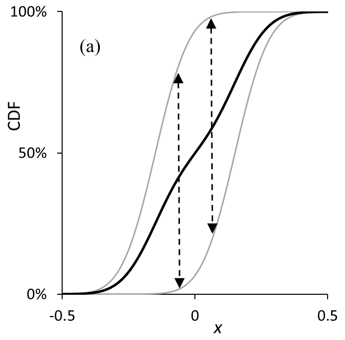
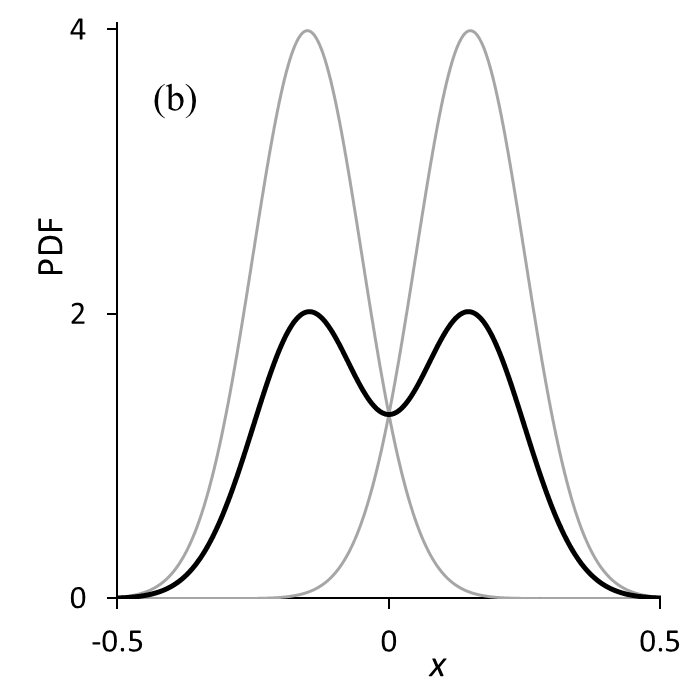
Figure 1: Vertical averaging (in black) of two Gaussian CDFs (in grey) in (a), and corresponding PDFs in (b).

Figure 2: Horizontal averaging (in black) of two Gaussian CDFs (in grey) in (a), and corresponding PDFs in (b).

In this paper, we consider a continuous random variable $x$. If we write the CDF and PDF of an individual forecast distribution as $F_{i}$ and $f_{i}$, respectively, (1) and (2) provide, respectively, the CDF and PDF of the vertical average of $k$ individual forecast distributions. For the PDF, (2) can be formally derived by differentiating with respect to (w.r.t.) $x$ the expression for the CDF in (1).

$$F_{V}(x) =\frac{1}{k}\sum_{i=1}^{k}F_{i}(x)$$ (1)

$$f_{V}(x) =\frac{1}{k}\sum_{i=1}^{k}f_{i}(x)$$ (2)

Given that horizontal averaging involves averaging quantiles, and the $\alpha$ quantile of an individual forecast distribution is $F_{i}^{-1}(\alpha)$, (3) provides the CDF resulting from horizontal averaging.

$$F_{H}^{-1}(\alpha)=\frac{1}{k}\sum_{i=1}^{k}F_{i}^{-1}(\alpha)$$ (3)

Bamber et al., (2016) show that differentiating each side of (3) w.r.t. $\alpha$ gives (4) for the PDF produced by horizontal averaging.

$$f_{H}\left((F_{H}^{-1}(\alpha)\right)=\frac{1}{\frac{1}{k}\sum_{i=1}^{k}1/f_{i}\left(F_{i}^{-1}(\alpha)\right)}$$ (4)

This expression indicates that horizontal averaging (i.e., averaging quantiles) leads to a distributional forecast for which the PDF, at the $\alpha$ quantile, is the harmonic mean of the PDFs of the individual distributional forecasts, each evaluated at their $\alpha$ quantile. Cooke, (2022) more concisely describes this as “harmonically averaging densities at the quantile points”, and notes that the harmonic mean of a set of values is strongly influenced by the smaller values of the set, which implies that for any chosen probability on the $y$-axis of a CDF, the slope of the resulting averaged CDF is strongly influenced by the CDFs with smallest slope at the same probability on the $y$-axis.

2.2 Is it better to Average Vertically or Horizontally?

Figures 1 and 2 illustrate the point, shown theoretically by Lichtendahl et al., (2013), that vertical averaging produces a distribution with greater variance than horizontal averaging. They suggest that the distributional forecast produced by vertical averaging will often be too wide, prompting them to propose horizontal averaging as a pragmatic alternative. In Section 4, we discuss in some detail several of the theoretical results provided by Lichtendahl et al., (2013), and consider the extension of these results to angular averaging. Using the distributional forecasts from the Federal Reserve Bank of Philadelphia’s Survey of Professional Forecasters, Lichtendahl et al., (2013) provide empirical results to support the use of horizontal averaging.

With other applications, it is not clear whether it is preferable to combine vertically or horizontally. For day-ahead electricity price forecasting, Uniejewski et al., (2019) and Marcjasz et al., (2020) find that vertical averaging is more accurate, while Uniejewski and Weron, (2021) obtain better results for horizontal averaging, with vertical averaging leading to distributions that are too wide. For forecasting wave height up to a day-ahead, Taylor and Jeon, (2018) report that vertical and horizontal averaging deliver similar accuracy. The fact that horizontal averaging delivers a distribution with lower variance than vertical averaging leads Bamber et al., (2016), Colson and Cooke, (2017) and Cooke, (2022) to express concern that horizontal averaging can result in overconfidence. Using data from multiple studies in a variety of applications involving expert judgments of probability distributions, they find vertical averaging noticeably more accurate than horizontal averaging.

In some applications, only a set of quantile forecasts are available (see, for example, Makridakis et al., 2022). Indeed, this is the case in our empirical study. In such situations, Cooke et al., (2021) and Cooke, (2022) acknowledge that horizontal averaging is easier, as vertical averaging requires a method to impute the complete distributional forecasts from the quantile predictions. Despite this, they warn against the use of horizontal averaging, citing its tendency to lead to distributions that underestimate the uncertainty.

2.3 Other Forms of Vertical and Horizontal Combining

Instead of using the simple average, distributional forecasts are often combined using weighted combinations. It is natural for the weights to reflect relative accuracy, measured using a proper scoring rule, such as the log score or continuous ranked probability score (CRPS). When applied in a vertical sense, such a weighted combination is sometimes termed the linear opinion pool (Stone, 1961) and has been described as the most popular approach to combining distributional forecasts (Knüppel and Krüger, 2022), with equal weighting viewed as a special case. Using weights in proportion to the log score of each forecast, Busetti, (2017) finds that horizontal combining is more accurate than vertical combining for quarterly economic growth and inflation. In a weighted horizontal combining method, Taylor and Taylor, (2023) set the weights to be inversely proportional to an approximation to the CRPS. If a different weighting scheme is considered desirable for different parts of the distribution, restrictions or adjustments would be needed to avoid quantile crossing (see, for example, Kapetanios et al., 2015; Kim et al., 2021).

The tendency for vertical combining to deliver overdispersed distributional forecasts has motivated nonlinear forms of vertical combining. The logarithmic opinion pool, which can be viewed as a geometric weighted average of PDFs, has been considered (see, for example, Busetti, 2017; Cooke, 2022; Satopää et al., 2014). Building on this, Gneiting and Ranjan, (2013) introduce generalized linear combinations, which involve a linear combination of distributional forecasts that have each been transformed using a link function. They also propose a beta-transformed linear pool that enables the combined distributional forecast to have a flexible variance, controlled by optimizing the parameters of the beta transformation.

Jose et al., (2014) use trimming to control the variance of the distribution resulting from vertical averaging. They suggest entire distributional forecasts can be trimmed based on the mean, or the trimming can be performed separately, in a vertical sense, for different values of the outcome variable (the CDF approach). After trimming, the remaining distributional forecasts are vertically averaged. Their exterior trimming approach reduces the impact of outlying distributions to reduce the variance of the resulting distribution, while their interior trimming approach has the opposite effect by reducing the impact of central lying distributions. Grushka-Cockayne et al., 2017b apply these ideas to the distributions produced by the trees in a quantile regression forest.

3 Angular Combining of Distributional Forecasts

3.1 Angular Averaging

With arguments in favor of both vertical and horizontal averaging, it becomes an empirical question as to which of the two approaches should be chosen for any given application. However, it could well be that neither vertical or horizontal averaging is ideal, and that there are useful aspects of each approach. For example, the unknown true density may be represented well by the tails produced by horizontal averaging and the central part of the distribution produced by vertical averaging.

In this paper, we propose an alternative averaging approach that allows the user to consider a range of possibilities between horizontal and vertical averaging. Our pragmatic alternative is to average on an angle that lies between these two extremes. We term this angular averaging. Figure 3(a) illustrates the idea with averaging of the same two Gaussian CDFs considered in Figures 1 and 2. Figure 3(a) shows angular averaging performed on a line that has been rotated clockwise by an angle of $\theta$ from the horizontal. Horizontal and vertical averaging are special cases of angular averaging, corresponding to $\theta$ being $0^{\textrm{o}}$ and $90^{\textrm{o}}$, respectively. Figure 3(a) shows horizontal, vertical and angular averaging performed from the point indicated by the white star on the left CDF. The three different forms of averaging each lead to averaging of this point with a different point on the right CDF. The result is three different averages, shown by the white, grey and black points.

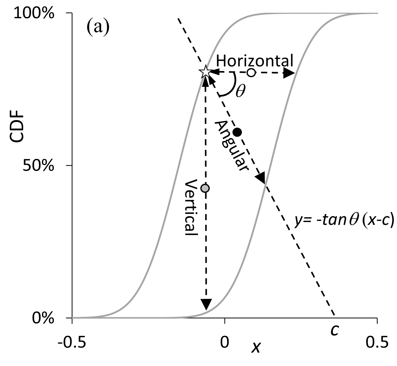
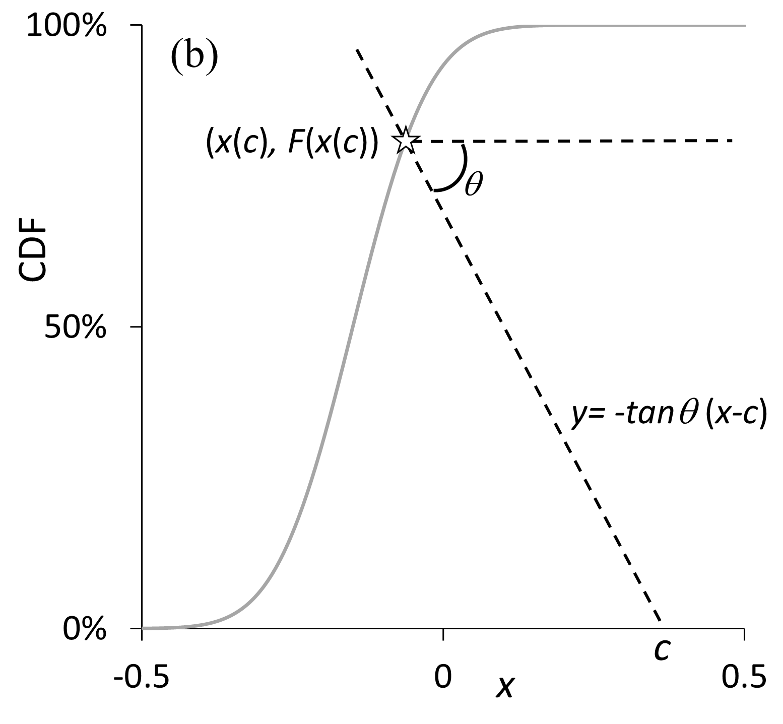
Figure 3: Angular, horizontal and vertical averaging of points on two Gaussian CDFs in (a), and illustration of our parameterization in (b).

Figure 3(b) illustrates our parameterization for angular averaging. For a fixed $\theta\in(0^{\textrm{o}},90^{\textrm{o}})$, consider a family of straight lines $y=-\tan\theta(x-c)$, where $-\tan\theta$ and $c\in(-\infty,\infty)$ are the gradient and $x$-intercept, respectively. We use $c$ to parameterize each CDF, and to enable a formal description of the CDF resulting from angular averaging. For any given CDF $F$, we define the point of intersection between the CDF curve $y=F(x)$ and the line $y=-\tan\theta(x-c)$ as $\left(x\left(c\right),F(x(c))\right)$. The function $x(c)$ is increasing w.r.t. $c$, and $\left(x\left(c\right),F(x(c))\right)$ covers the entire CDF as $c$ ranges from $-\infty$ to $\infty$. Thus, the set of points $\left(x\left(c\right),F(x(c))\right)$ provides a parameterization of the CDF using $c$. That is, each point on the CDF can be uniquely identified by a single value of $c$. Indeed, $F(x(c))$ is a function of $c$ that behaves as a CDF.

Using this parameterization for each of k CDFs, $F_{i}$, we have k points of intersection $\left(x_{i}\left(c\right),F_{i}(x_{i}(c))\right)$ between the CDFs and the line $y=-\tan\theta(x-c)$. Averaging the $k$ points $\left(\frac{1}{k}\sum_{i=1}^{k}x_{i}(c),\frac{1}{k}\sum_{i=1}^{k}F_{i}(x_{i}(c))\right)$ yields the CDF $F_{A,\theta}$ of the angular average at $\frac{1}{k}\sum_{i=1}^{k}x_{i}(c)$,

$$F_{A,\theta}\left(\frac{1}{k}\sum_{i=1}^{k}x_{i}(c)\right)=\frac{1}{k}\sum_{i=1}^{k}F_{i}(x_{i}(c)).$$ (5)

We note that (5) contains $\frac{1}{k}\sum_{i=1}^{k}x_{i}(c)$ and $\frac{1}{k}\sum_{i=1}^{k}F_{i}(x_{i}(c))$, which represent horizontal and vertical averaging, respectively, implying that both of these forms of averaging are present in angular averaging. The PDF $f_{A,\theta}$ of the angular average is provided by Proposition 3.1. The proof of this proposition is presented in the appendix. If $\theta=0$, $f_{A,\theta}$ reduces to harmonic averaging of the PDFs, as in (4) for horizontal averaging. As $\theta$ increases and approaches $90^{\textrm{o}}$, implying that all the $x_{i}$ take the same value, $f_{A,\theta}$ converges to the arithmetic average of the PDFs, as in (2) for vertical averaging.

Proposition 3.1

$f_{A,\theta}\left(\frac{1}{k}\sum_{i=1}^{k}x_{i}(c)\right)=\left(\sum_{i=1}^{k}\frac{f_{i}\left(x_{i}(c)\right)}{f_{i}\left(x_{i}(c)\right)+\tan\theta}\right)\Big{/}\left(\sum_{i=1}^{k}\frac{1}{f_{i}\left(x_{i}(c)\right)+\tan\theta}\right).$

We also note that, although our parameterization is w.r.t. the $x$-intercept $c$ of the angled line, we could have chosen to parameterize w.r.t. the $y$-intercept of this line. Indeed, this would be needed for horizontal averaging, as there is no $x$-intercept when the angled line is horizontal.

We have two comments to make regarding the angle $\theta$. Firstly, if and only if $\theta$ is an angle in the range $\left[0^{\textrm{o}},90^{\textrm{o}}\right]$, will the function resulting from angular averaging be guaranteed to be monotonic and take values in the range [0,1], which are the necessary conditions for a CDF. If $\theta$ was not a value in the range $\left[0^{\textrm{o}},90^{\textrm{o}}\right]$, the angled line in Figure 3 could be crossed more than once by one of the CDFs to be combined. A second comment regarding the angle $\theta$ is that it is a parameter that should, ideally, be estimated using historical data. For many applications, past data is available, and so the estimation of a single parameter is not particularly burdensome. Indeed, the need for parameter estimation is also an aspect of many other combining methods. Furthermore, even though horizontal and vertical averaging require no parameter estimation, to decide which of these two methods to use, there is a need for a sample of past data with which to compare historical accuracy.

Figure 4 shows the CDF, and corresponding PDF, resulting from angular averaging of the same two Gaussian CDFs considered in Figures 1 to 3. The averaging has been performed at an angle of $45^{\textrm{o}}$, as conveyed by the dashed lines in Figure 4(a). For a variety of different values of $\theta$, Figure 5(a) shows the different CDFs that result from angular averaging of the two Gaussian CDFs. Figure 5(b) provides the corresponding PDFs resulting from angular averaging. As we noted when discussing Figures 1(b) and 2(b), the PDFs resulting from vertical and horizontal averaging of the two Gaussian CDFs are bimodal and unimodal, respectively. It is interesting to note that, for the example we are using, it is only when $\theta$ exceeds about $85^{\textrm{o}}$ that the angular averaging of the two CDFs leads to a PDF that is bimodal. This suggests that it would be wise in empirical studies to implement angular averaging for different values of $\theta$ spanning the full range from $0^{\textrm{o}}$ to $90^{\textrm{o}}$. In our empirical study of Section 5, as candidate values for $\theta$, we considered each integer value from $0^{\textrm{o}}$ to $90^{\textrm{o}}$.

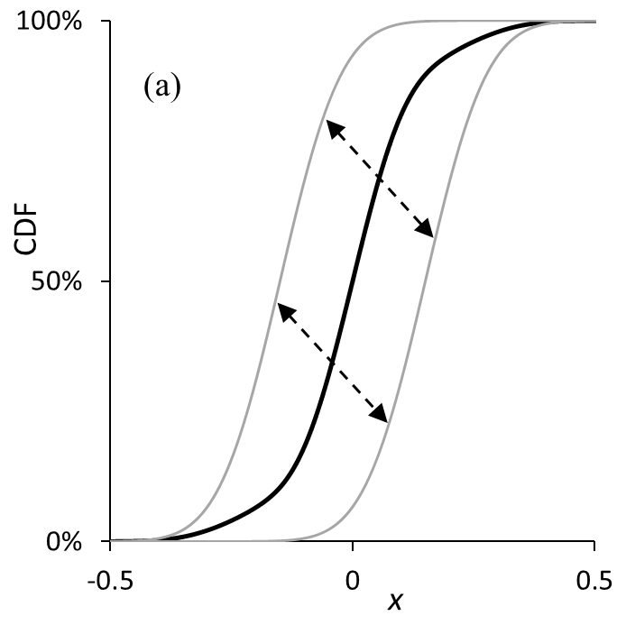
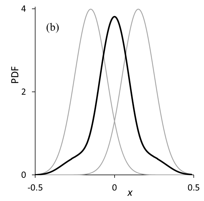
Figure 4: Angular combining (in black) of two Gaussian CDFs (in grey) in (a), and corresponding PDFs in (b). Averaging is performed at an angle $\theta=45^{\textrm{o}}$, as indicated by the dashed lines.

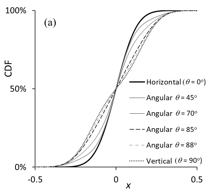
Figure 5: Horizontal, vertical and angular averaging of two Gaussian CDFs. Angular averaging performed for $\theta=45^{\textrm{o}}$, $70^{\textrm{o}}$, $85^{\textrm{o}}$ and $88^{\textrm{o}}$. CDFs in (a) and PDFs in (b).

In Section 2.1, we commented that horizontal and vertical combining cannot be applied if any part of an individual CDF forecast is horizontal or vertical, respectively. We note that this is not a limitation of angular combining (for $0^{\textrm{o}}<\theta<90^{\textrm{o}}$).

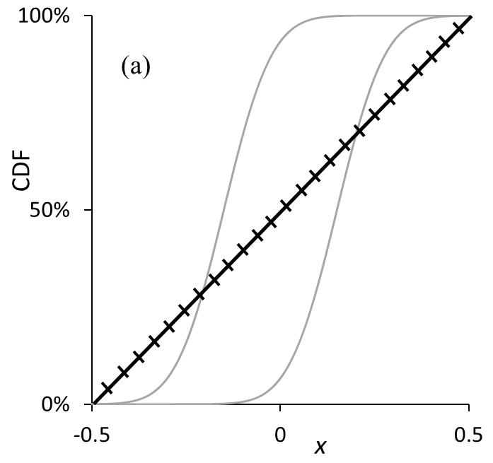
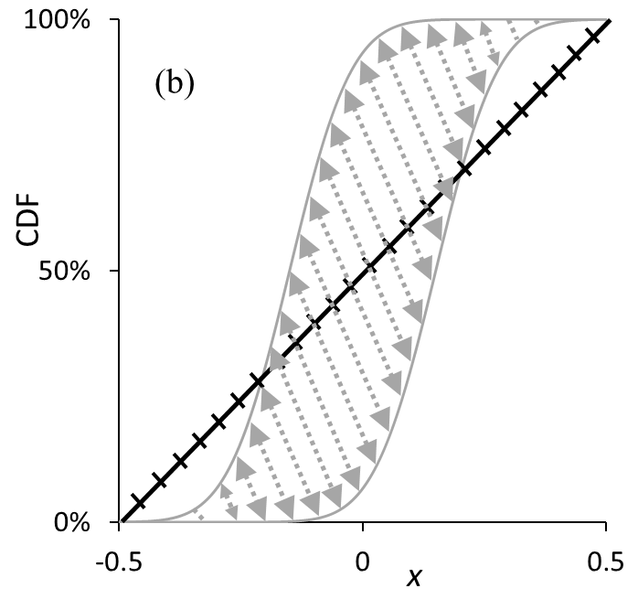
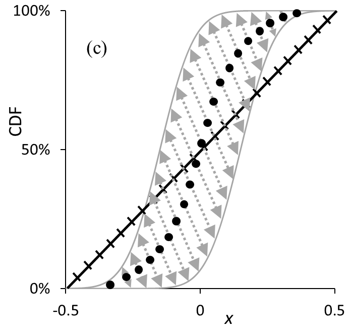
Figure 6: Implementation of angular averaging of two Gaussian CDFs. In (a), a diagonal straight line is drawn (in black), and on it are marked many evenly spaced points. In (b), an angled straight line at angle $\theta=65^{\textrm{o}}$ is drawn (in grey) through each marked point and between the two CDFs. In (c), the midpoint of each angled straight line is obtained, and these midpoints map out the new CDF.

3.2 Practical Implementation of Angular Averaging

To implement angular averaging, a numerical approach can be used. For the averaging of two CDFs, Figure 3(a) shows that each point on the new CDF is the midpoint on an angled straight line between the individual CDFs being combined. To obtain the midpoint requires the points of intersection of the angled straight line with the two CDFs. It is in obtaining these points of intersection that a numerical procedure can be used. The new CDF can be constructed by finding the midpoint on a set of angled straight lines across the range of the support of the CDFs. This is illustrated in Figure 6 for the same two Gaussian CDFs averaged in our previous figures. Notice that we have scaled the $x$-axes so that they each have unit length. This enables us to compare more easily values of the angle $\theta$ used for applications to different data. For CDFs with unbounded support, we would pragmatically suggest the scaled $x$-axis of unit length extends to at least the 1% and 99% quantiles of each CDF.

Figure 6(a) shows that our approach proceeds by drawing a diagonal straight line (in black) from the bottom left to the top right of the plot. We mark $m$ equally spaced points on the line. As shown in Figure 6(b), we then draw an angled straight line (in grey) through each of these $m$ points. Each of these angled straight lines is, as shown in Figure 3, at an angle $\theta$ to the horizontal. We have chosen $\theta=65^{\textrm{o}}$ for the angled lines (in grey) in Figure 6. After obtaining the points of intersection of each angled straight line with the CDFs, we note the midpoint, as shown in Figure 6(c). To produce the new CDF, for simplicity, we use linear interpolation between these midpoints. In our empirical work, we used $m=1001$, which was sufficiently large to deliver a relatively smooth CDF. When the angular averaging is applied to $k$ CDFs, where $k>2$, the procedure is the same, except that the averaging is applied to the $k$ points of intersection of each angled straight line with the $k$ CDFs.

3.3 Angular Averaging as Generalized Linear Averaging

A useful way to understand angular averaging is through the framework of the generalized linear combination considered by Dawid et al., (1995) and Gneiting and Ranjan, (2013). For generalized linear averaging, with the CDF denoted as $F_{GL,h}$, the combination has the following form,

$$h\left(F_{GL,h}(x)\right)=\frac{1}{k}\sum_{i=1}^{k}h(F_{i}(x))$$ (6)

where $h$ is a continuous and strictly increasing link function. In simple terms, the transformed $F_{GL,h}$ under $h$ is the vertical average of the transformed $F_{i}$ under $h$. Angular averaging can be viewed as similar in spirit, but with the notable differences that a particular link function is used, and it is applied to the quantiles instead of the CDFs.

Recall that in Section 3.1, for any CDF $F$, we introduced a parameterization w.r.t. the $x$-intercept $c$ of the line $y=-\tan\theta(x-c)$. We noted that as $c$ ranges from $-\infty$ to $\infty$, $F(x(c))$ increases from 0 to 1, making it possible to view $F(x(c))$ as a function of $c$ that behaves as a CDF. Let us now write this function of $c$ as $h_{\theta}(F)$, where $h_{\theta}$ can be viewed as a link function. For any probability level $\alpha\in[0,1]$, we can then write $c=h_{\theta}(F)^{-1}(\alpha)$. For this probability level, we can also consider the point of intersection of the line $y=-\tan\theta(x-c)$ with the CDF curve $y=F(x)$ by substituting $y=\alpha$ and $x=F^{-1}(\alpha)$ into the equation of the line to give $\alpha=-\tan\theta(F^{-1}(\alpha)-c)$, which can be rearranged as $c=F^{-1}(\alpha)+\frac{\alpha}{\tan\theta}$. Equating the two expressions for $c$, we find that the link function $h_{\theta}$ defines a quantile transformation,

$$h_{\theta}(F)^{-1}(\alpha)=F^{-1}(\alpha)+\frac{\alpha}{\tan\theta}\quad\quad\forall\alpha\in[0,1].$$ (7)

Based on this, we can reinterpret the angular averaging in (5) within a framework similar to (6),

$$h_{\theta}\left(F_{A,\theta}\right)(c)=\frac{1}{k}\sum_{i=1}^{k}h_{\theta}(F_{i})(c)\quad\quad\forall c\in(-\infty,\infty).$$ (8)

This interpretation is illustrated in Figure 7 for the angular averaging of two CDFs in light grey, $F_{1}$ and $F_{2}$. Figure 7 shows $F_{1}$ and $F_{2}$ transformed using $h_{\theta}(F)^{-1}(\alpha)=F^{-1}(\alpha)+\frac{\alpha}{\tan\theta}$ to give two new CDFs in dark grey, $h_{\theta}(F_{1})$ and $h_{\theta}(F_{2})$. The light grey point on the angled line is the angular average of the points of intersection of the angled line with the two light grey CDFs. The transformation of this light grey point results in the black point, which is also the vertical average of the two new, dark grey CDFs at $x=c$.

Alternatively, we can use the $y$-intercept instead of the $x$-intercept in the parameterization discussed in Section 3.1, i.e., we can consider a family of lines defined as $y=-x\tan\theta+c$. This parameterization yields the following alternative version of (8),

$$\tilde{h}_{\theta}\left(F_{A,\theta}\right)^{-1}(c)=\frac{1}{k}\sum_{i=1}^{k}\tilde{h}_{\theta}(F_{i})^{-1}(c)\quad\quad\forall c\in(-\infty,\infty).$$ (9)

where $\tilde{h}_{\theta}(F)(x)=F(x)+x\tan\theta\ \forall x\in(-\infty,\infty)$. That is, the transformed CDF $\tilde{h}_{\theta}\left(F_{A,\theta}\right)$ is the horizontal average of $\tilde{h}_{\theta}(F_{i})$. The derivation of (9) is similar to that for (8), hence is omitted here.

Note that unlike $h_{\theta}(F)$, $\tilde{h}_{\theta}(F)$ is not a CDF since it is unbounded. Hence, (8) is a more useful and convenient interpretation. In the appendix, we use (8) to prove some of the main theoretical results in Section 4. Finally, we emphasize that (8) and (9) further show that angular averaging contains elements of both vertical and horizontal averaging.

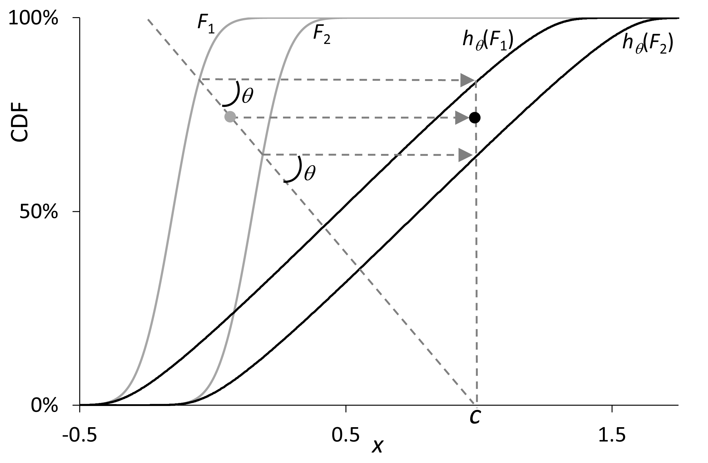
Figure 7: Visual illustration of angular averaging as generalized linear averaging. The light grey point is the angular average of the points of intersection of the angled line with the two CDFs, $F_{1}$ and $F_{2}$. The transformation of this light grey point results in the black point, which is also the vertical average of the two transformed CDFs, $h_{\theta}(F_{1})$ and $h_{\theta}(F_{2})$, at the point $x=c$.

3.4 Other Forms of Angular Combining

In comparing horizontal, vertical and angular combining, we have focused on the simple average. However, CDFs have been combined horizontally and vertically using other approaches, as we discussed in Section 2.3. We suggest that such aggregation methods can be applied on an angle. As an example, in our empirical study of Section 5, we consider a combining method that weights forecasts inversely proportional to the CRPS, and implement this horizontally, vertically and at angles between $0^{\textrm{o}}$ and $90^{\textrm{o}}$. To implement the angular weighted combination, for each grey angled straight line in Figure 6(c), we calculate a weighted average of the points of intersection of the angled straight line with the CDFs.

4 Theoretical Results

In this section, we present results concerning the mean, variance, shape and CRPS of the distributional forecast resulting from angular averaging. We also consider the distribution produced by an angular form of median combining. All proofs are postponed to the appendix.

4.1 Mean of the Angular Average

Lichtendahl et al., (2013) show that, for vertical and horizontal averaging, the means of their resulting distributions both equal the average of the means of the individual distributions. Proposition 4.1 indicates that this is also true for the distribution produced by angular averaging.

Proposition 4.1

The mean of the angular average $F_{A,\theta}$ is identical to the average of the means of the individual distributions $F_{i}$ in the combination. Therefore, the means of horizontal, vertical and angular averaging are identical.

4.2 Variance and Shape of the Angular Average

A distributional forecast with lower variance than another is described as being sharper. Lichtendahl et al., (2013) prove that horizontal averaging produces a distributional forecast that is sharper than the one produced by vertical averaging. We now extend this result to angular averaging.

Theorem 4.2

The angular average $F_{A,\theta}$ is sharper than the vertical average $F_{V}$.

Theorem 4.2 implies that the angular and horizontal averages are both sharper than the vertical average. As angular averaging conceptually lies between vertical and horizontal averaging, it is natural to ask whether the variance of the angular average falls between the variances of the vertical and horizontal averages. While this may not hold generally, we now explain that it is true in the specific scenario described in Assumption 4.2,

Each individual distribution $F_{i}$ in the combination has the same scale and is from the same location-scale family, where the PDF of the standardized member of the location-scale family is symmetric about 0 and unimodal.

These assumptions are among those adopted in Proposition 5 of Lichtendahl et al., (2013), which compares the CDFs for vertical and horizontal averaging. Our Lemma 4.3 below extends the proposition to angular averaging, although the lemma relates to the averaging of just two CDFs.

Lemma 4.3

Under Assumption 4.2, when two distributions are averaged, the PDF $f_{A,\theta}$ of angular averaging is symmetric about its mean, and $F_{A,\theta}(x)$ is increasing w.r.t. $\theta$ when $x$ is below the mean, and $F_{A,\theta}(x)$ is decreasing w.r.t. $\theta$ when $x$ is above the mean.

The implication of Lemma 4.3 for the shape of the CDF resulting from angular averaging is illustrated in Figure 5(a). In terms of the PDF produced by angular averaging, Lemma 4.3 indicates that, for angular averaging, the gradient of the resulting CDF at its mean is decreasing w.r.t. $\theta$, which implies that the PDF at the mean is decreasing w.r.t. $\theta$. Figure 5(b) shows the center of the PDF reducing w.r.t. $\theta$, and, correspondingly, the density in the tails increasing w.r.t. $\theta$. Our comments here on the shape of the CDF produced by angular averaging extend the discussion of Lichtendahl et al., (2013) regarding the shape of the CDF resulting from horizontal and vertical averaging, and in particular their Proposition 11.

Lemma 4.3 implies that $F_{A,\theta}^{-1}(\alpha)-\mathbb{E}_{X\sim F_{A,\theta}}\left[X\right]$ is negative and decreasing w.r.t. $\theta$ for $\alpha<\frac{1}{2}$, and is positive and increasing w.r.t. $\theta$ for $\alpha>\frac{1}{2}$. Expressing the variance of a CDF $F$ as $\intop_{0}^{1}\left(F^{-1}(\alpha)-\mathbb{E}_{X\sim F}\left[X\right]\right)^{2}d\alpha$, Lemma 4.3 implies that the variance of the angular average $F_{A,\theta}$ of two CDFs is monotone increasing w.r.t. $\theta$. Theorem 4.4 builds on Lemma 4.3 to show that the variance of the angular average $F_{A,\theta}$ is increasing w.r.t. $\theta$, regardless of the number of CDFs included in the averaging. This means that the horizontal average $F_{H}$ is the sharpest distribution, the vertical average $F_{V}$ is the least sharp, and the angular average $F_{A,\theta}$ is between $F_{H}$ and $F_{V}$ in terms of sharpness. An implication of this is that, as the average level of confidence of a set of forecasters increases, moving from underconfidence to overconfidence, it is preferable to increase the angle $\theta$ used in angular averaging from $0^{\textrm{o}}$ to $90^{\textrm{o}}$.

Theorem 4.4

Under Assumption 4.2, the variance of $F_{A,\theta}(x)$ is increasing w.r.t. $\theta$.

4.3 Score of the Angular Average

Lichtendahl et al., (2013) show that the score for vertical averaging is no greater than the average of the scores of the individual distributions for the linear score, log score, quadratic score and CRPS. They show that this is also true for the linear and log scores when it comes to horizontal averaging. Although, for the quadratic score, the result is not necessarily valid for horizontal averaging, the authors establish conditions under which it is true. They do not discuss the result for horizontal averaging for the CRPS. In this paper, we address this, and also extend the result to angular averaging.

Let us first present the definition of the CRPS before we present our results in Theorem 4.5. For a CDF $F$ and corresponding realization $z$, the CRPS can be written in the following two forms,

$$CRPS(F,z) =\intop_{\infty}^{\infty}\left(F(x)-\mathbbm{1}(x>z)\right)^{2}dx$$ (10)

$$=-\frac{1}{2}\mathbb{E}_{X,X^{{}^{\prime}}\sim F}\big{|}X-X^{{}^{\prime}}\big{|}+\mathbb{E}_{X\sim F}\big{|}X-z\big{|}$$ (11)

where $X$ and $X^{{}^{\prime}}$ indicate two independent random variables with CDF $F$.

Theorem 4.5

The CRPS for the vertical, horizontal and angular averages are less than or equal to the average of the CRPS of the individual distributional forecasts $F_{i}$ in the combination.

Lichtendahl et al., (2013) base their proof of this result for vertical averaging on (10). By contrast, in our proof of Theorem 4.5, we use (11). The proof offers useful insight into angular averaging. Loosely speaking, in comparison with the average CRPS of the individual distributions, the lower CRPS for vertical averaging is solely due to the first term in (11), the lower CRPS for horizontal averaging is solely because of the second term in (11), and the lower CRPS for angular averaging is due to both the first and second terms in (11). This finding supports our earlier comments that angular averaging has aspects of both vertical and horizontal averaging.

4.4 Angular Median

Hora et al., (2013) consider the median as a robust alternative to averaging distributional forecasts. They show that obtaining the median horizontally and vertically results in the same distributional forecast. Similarly to angular averaging, the median can also be obtained at any angle $\theta$. In other words, to construct the angular median CDF for a chosen angle $\theta$, we find the median of the points of intersection of the individual CDFs with an angled line $y=-\tan\theta(x-c)$, and repeat this for different values of $c\in(-\infty,\infty)$. Theorem 4.6 shows that, if there is an odd number of individual distributions, the same CDF is produced when the median is obtained vertically, horizontally or at an angle.

Theorem 4.6

When $k$ is odd, obtaining the median of $k$ CDFs, horizontally, vertically or at an angle $\theta$ produces the same CDF.

5 Empirical Study

In this section, we use mortality data to evaluate our proposed approach to distributional forecast combining. We introduce the data, present the forecast evaluation measures that we use, describe the combining methods that we implemented, and finally present the results.

5.1 The Dataset

We used data from the COVID-19 Forecast Hub (COVID-19 Forecast Hub 2020). The Hub provides open access to weekly observations and forecasts from multiple forecasting teams for one to four weeks-ahead for the number of reported COVID-19 deaths at the national and state level in the U.S. Mortality forecasts have been used by public health decision makers during the pandemic (Adam, 2020; Nikolopoulos et al., 2021; Ray et al., 2020). Forecasts from the Hub have gained widespread attention with weekly updates presented on the website of the Center for Disease Control and Prevention, as well as featuring on Nate Silver’s FiveThirtyEight website. The teams submitting forecasts to the Hub come from academia, industry and government affiliated groups. We used forecasts of the number of weekly COVID-19 deaths produced from the 84 weekly forecast origins from 6 June 2020 to 8 January 2022, inclusive, and mortality observations, recorded on 15 January 2022, for the weeks ending 13 June 2020 to 15 January 2022, inclusive. We considered mortality at the national level, for the 50 states, and for the District of Columbia, which for simplicity we refer to as a state. The dataset, therefore, involved 52 time series. Taylor and Taylor, (2022) used the same data in a study of interval forecast combining.

The curators of the Hub invite forecasting teams to submit a point forecast and quantile forecasts corresponding to the following 23 probability levels: 1%, 2.5%, 5%, 10%, 15%, 20%, 25%, 30%, 35%, 40%, 45%, 50%, 55%, 60%, 65%, 70%, 75%, 80%, 85%, 90%, 95%, 97.5% and 99%. As our interest in this paper is in distributional forecasts, we constructed continuous CDFs from the 23 quantiles. To do this, we used the following simple approach: we defined the lower bound of the distribution as being a distance below the 1% quantile equal to the difference between the 1% and 2.5% quantiles (unless this resulted in a negative lower bound, in which case we set it to be zero); we defined the upper bound of the distribution as being a distance above the 99% quantile equal to the difference between the 97.5% and 99% quantiles; and we used linear interpolation to give the CDF between each pair of quantiles, between the lower bound and the 1% quantile, and between the 99% quantile and the upper bound. (Defining the lower and upper bounds as the 1% and 99% quantiles, respectively, produced very similar out-of-sample results for the evaluation measures we describe in Section 5.2.) Each week, the curators of the Hub generate an “ensemble” forecast combination. Initially, the ensemble was the horizontal average; from mid-July 2020, it was computed as the median; and after mid-November 2021, it was a horizontal weighted combination. At each forecast origin, for each series, the curators of the Hub screen forecasting teams for inclusion in their ensemble, removing teams if their forecasts are clearly unrealistic. We used only the remaining eligible teams in our study. There was variation over time in the identity and number of teams. In Figure 8, for each forecast origin, a box plot summarizes the differing number of eligible teams for each of the 52 series. About half the teams used compartmental models. The others employed statistical methods, machine learning or agent-based models. The diversity of methods motivates attempts to extract wisdom from the crowd (see Surowiecki, 2004).

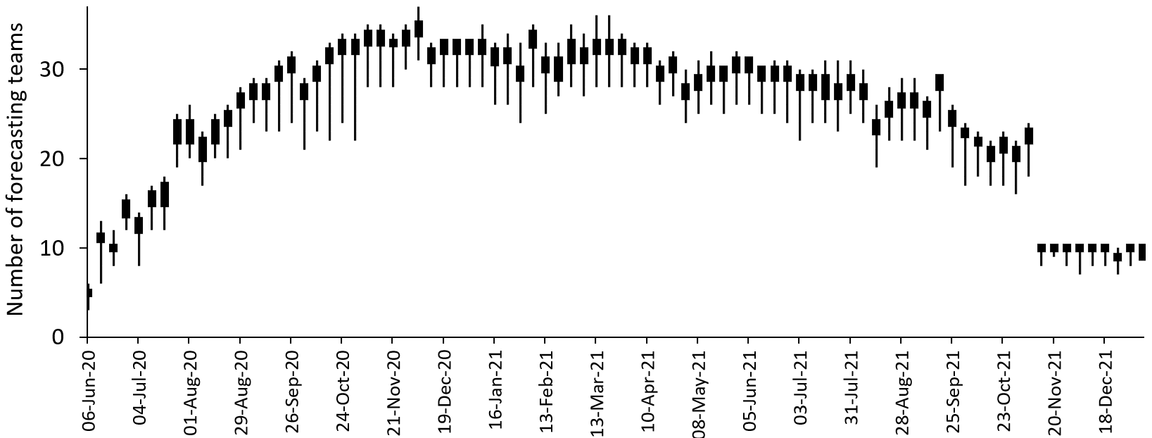
Figure 8: For each of the 84 forecast origins, the box plot summarizes the number of eligible forecasting teams for each of the 52 series.

5.2 Structure of the Study and Evaluation Measures

We used forecasts made from the first 10 out of the 84 forecast origins for the initial in-sample parameter estimation. For the remaining 74 forecast origins, we used an expanding in-sample period consisting of all weeks up to and including the origin itself. Out-of-sample forecasts were, therefore, produced for the final 74 weeks of each of the 52 mortality time series.

In terms of out-of-sample evaluation, the aim of distributional forecasting is to maximize sharpness subject to calibration. Sharpness relates to the concentration of the distributional forecast, while calibration measures its statistical consistency with the data (Gneiting and Katzfuss, 2014). We report unconditional calibration using reliability diagrams and the percentage of observations falling within 95% and 50% intervals obtained from the distributional forecasts. Evaluating these intervals provides insight into forecast accuracy for the central and tail regions of the distributions (Makridakis et al., 2022).

We use the following mean quantile score (MQS) to assess distributional forecast accuracy,

$$\frac{1}{23}\sum_{i=1}^{23}2\left(\alpha_{i}-I\left\{x\leq F^{-1}(\alpha_{i})\right\}\right)\left(x-F^{-1}(\alpha_{i})\right)$$

where $x$ is the observation, $F^{-1}(\alpha_{i})$ is the quantile with probability level $\alpha_{i}$, and $I\{\cdot\}$ is the indicator function. Using the Gneiting and Ranjan, (2011) definition of the quantile score, the MQS is the mean of the quantile scores for the 23 probability levels. A score is proper if its expectation is minimized when the forecast is correct, and is strictly proper if the correct forecast is the unique minimizer (Gneiting and Katzfuss, 2014). Proper scores assess both calibration and sharpness. The MQS is a strictly proper score for the 23 quantiles and a proper score for the distribution (Grushka-Cockayne et al., 2017b ; Jose and Winkler, 2009). The MQS approximates the CRPS. We use the MQS rather than the CRPS itself, as the MQS is employed in other studies of the COVID-19 Forecast Hub data, which reflects the focus of the Hub on forecasting the 23 quantiles (see, for example, Bracher et al., 2021a , Bracher et al., 2021b ).

As the Hub elicits forecasts of 23 quantiles, rather than the full CDF, only horizontal combining approaches have previously been considered for this data. By using the MQS, we also focus on the 23 quantiles, so that our study essentially investigates whether converting the 23 quantiles into a CDF and then performing vertical or angular combining can be beneficial, even if only the accuracy of the 23 quantiles is of interest. The idea of converting a set of quantile forecasts into a continuous CDF to enable the use of a broader set of combining methods parallels the “probability averaging” approach to interval forecast combining proposed by Gaba et al., (2017).

To evaluate 95% and 50% intervals obtained from the distributional forecasts, in addition to calibration, we use the interval score of Winkler, (1972). For a $(1-\alpha)\times 100\%$ interval, the score is

$$(u-l)+\frac{2}{\alpha}I\{x\leq l\}(l-x)+\frac{2}{\alpha}I\{x\geq u\}(x-u)$$

where $l$ is the interval’s lower bound $F^{-1}(\alpha/2)$, and $u$ is its upper bound $F^{-1}(1-\alpha/2)$.

In addition to averaging each score over the out-of-sample period, we also averaged over the lead times, as the relative performances of the methods were similar for the four lead times, and the series were relatively short. We report the scores averaged across all 52 series, but as this will be heavily influenced by the higher mortality series, we also report results for the following four groupings of the series: the U.S. national level series; the 17 states for which cumulative mortality was highest in the final week of the dataset; the 17 states with the next highest cumulative mortality in the final week; and the 17 states with lowest cumulative mortality in the final week.

We also computed skill scores, defined as the percentage by which a method is more accurate than a benchmark, which we chose to be horizontal averaging. Skill scores provide a further way of avoiding higher mortality series dominating when averaging across series. To average over skill scores, we first calculated the geometric mean of the ratios of the score for each method to the score for the benchmark method, then subtracted this from 1, and multiplied the result by 100.

5.3 Implementing Horizontal, Vertical and Angular Combining

We implemented horizontal, vertical and angular averaging, as well as horizontal, vertical and angular forms of performance-based weighted combining. As in the horizontal combining study of Taylor and Taylor, (2023), we set the combining weight to be inversely proportional to the team’s in-sample MQS. If fewer than five past periods were available from which to produce the in-sample MQS for a team, the MQS was assumed equal to the average of the MQS of the other teams in the combination. Note that the weights only approximately reflect relative performance because the MQS will typically not have been computed from the same past periods for all teams, due to inconsistencies in the record of submissions among the teams.

Our implementation of horizontal averaging and horizontal weighted combining simply involved combining the quantile forecasts for each of the 23 probability levels. Vertical combining involved averaging and weighted combining of the probability forecasts for each of a set of values of the mortality variable $x$. We chose this set of $x$ values to consist of all 23 quantile forecasts submitted by all the teams. For each value of $x$, we combined the probability forecasts obtained from each team’s distributional forecast.

In Section 3.2, with reference to Figure 6(c), we described how angular averaging involves, for each of the $m$=1001 angled straight lines (in grey), averaging the points of intersection of the angled straight line with the distributional forecasts. For each angled straight line, in addition to averaging, we applied the performance-based weighted combination, using the same weights we had used for horizontal and vertical weighted combining. We then optimized the angle $\theta$ separately for angular averaging and angular weighted combining. For each series and method, at each forecast origin, we optimized $\theta$ by minimizing the in-sample MQS averaged over the four lead times. Figure 9 provides examples of the CDF forecasts produced by the individual teams and by horizontal, vertical and angular averaging. The examples correspond to the forecasts produced from the final forecast origin in our dataset for California and New York State. For each state, the figure shows that the CDF forecasts of the teams vary quite considerably in terms of their location, spread and shape. We can also see differences between the CDFs produced by the three forms of averaging.

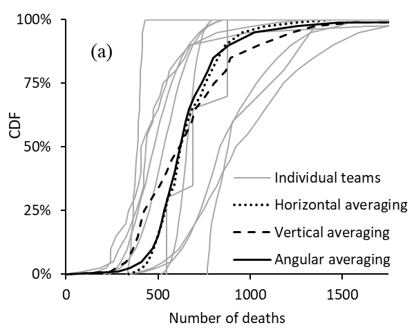
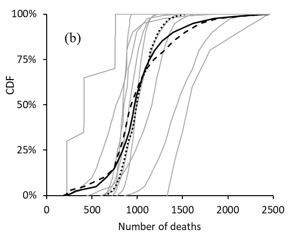
Figure 9: 1 week-ahead CDF forecasts for 15 January 2022 from 10 individual teams and the three averaging methods for (a) California, and (b) New York State. For angular averaging, the optimized angle $\theta$ was $60^{\textrm{o}}$ for California and $79^{\textrm{o}}$ for New York.

In a small number of cases, forecasting teams submitted CDF forecasts for which the quantiles were identical for two or more adjacent values of the 23 probability levels. For example, this is the case for the left-most CDF forecast in Figure 9(b). As we mentioned in Section 2.1, this is problematic for vertical combining because, for certain values on the $x$-axis, there is a set of CDF values, rather than a single value. To address this, for any such value on the $x$-axis, we simply averaged the set of CDF values before applying vertical combining.

With optimization of the angle $\theta$ performed at each forecast origin, angular combining essentially allows switching between different angles as the method is passed through the out-of-sample period. To challenge this, we implemented a method that allowed switching between only horizontal and vertical combining, with the choice dictated by in-sample MQS. We refer to this as horizontal/vertical switching.

As our focus in this paper is on horizontal, vertical and angular combining, we initially report results for only these methods. In Section 5.9, we present results for other combining methods.

A comparison of the results of the combining methods with those of individual teams is not straightforward because none of the teams provided forecasts that passed the Hub’s eligibility screening for all past periods and series. In view of this, we focus only on combining methods in our analysis.

5.4 Results for Angular Combining with a Fixed Angle

As an initial investigation into suitable values of the angle $\theta$ used in angular combining, we evaluated the accuracy of the approach when $\theta$ was not optimized but was fixed at the same value for all 74 forecast origins used to produce out-of-sample forecasts. We did this, in turn, for integer values of $\theta$ between $0^{\textrm{o}}$ and $90^{\textrm{o}}$. For angular averaging, Figure 10 presents the resulting MQS skill scores, computed for the five categories of series: all 52 series, the U.S. national level series, and the high, medium and low mortality groupings of series. Higher values of the skill score are preferable. First note that the extreme left of the figure corresponds to horizontal averaging, and as this is the benchmark method in the skill score calculation, the skill scores are all zero at this left extreme. The right extreme ($\theta=90^{\textrm{o}}$) corresponds to vertical averaging. For the U.S. national level series, the figure shows the skill score a little above zero for values of $\theta$ up to about $60^{\textrm{o}}$, beyond which the skill score reduces to a low negative value at $\theta=90^{\textrm{o}}$, indicating vertical averaging is not suitable for this mortality series. For the other four categories of series, the other four lines in Figure 10 show positive skill scores for values of $\theta$ above zero, indicating that angular averaging with any angle above zero was more accurate than horizontal averaging. These four lines all peak with $\theta$ between about $80^{\textrm{o}}$ and $85^{\textrm{o}}$, suggesting that angular averaging with an angle in this range would be suitable for series in these four categories, and that it would be more accurate than vertical averaging ($\theta=90^{\textrm{o}}$). For these four categories, the skill score is positive at $\theta=90^{\textrm{o}}$, implying that vertical averaging outperformed horizontal averaging. Therefore, of the five categories of series, it is only for the U.S. national series that horizontal averaging outperforms vertical averaging. The theoretical results of Lichtendahl et al., (2013) suggest that this may be because, for this particular series, vertical averaging produced overly wide distributions, due to the individual distributional forecasts either having variances that are too large or diverse locations. We return to this when we consider results for calibration in Section 5.8.

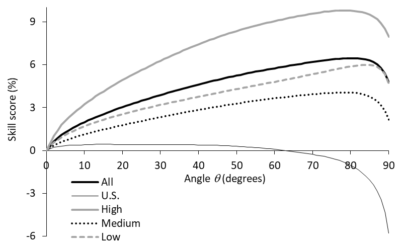
Figure 10: MQS skill score for the out-of-sample period for angular averaging at different angles. Higher values of the skill score are better.

The message from Figure 10 that relatively high values for $\theta$ tended to be most suitable is interesting because, for the two Gaussian CDFs in Figure 5, an informal conclusion could be that the CDF resulting from angular averaging only became very noticeably different to horizontal averaging for values of $\theta$ above about $70^{\textrm{o}}$. However, such a conclusion from Figure 5 ignores the tails, which are noticeably different for much lower values of $\theta$. It should also not be overlooked that Figure 10 presents the MQS, which summarizes accuracy for the full distribution. This motivates a more careful consideration of the tails of the distribution produced by angular averaging, and for this we turn to the interval score.

For the 95% interval skill score, Figure 11 presents the analogy of Figure 10. By contrast with the MQS skill score results in Figure 10, Figure 11 shows that for the 95% interval skill score the greatest accuracy resulted when $\theta$ was between $15^{\textrm{o}}$ and $40^{\textrm{o}}$, and that high values of $\theta$ produced poor accuracy. In this paper, for simplicity, we optimize $\theta$ using the MQS. However, Figures 10 and 11 suggest that, if interval forecast accuracy is the priority, the choice of $\theta$ should be driven by the interval score. For angular weighted combining, we produced the analogous figures to Figures 10 and 11, and found similar results.

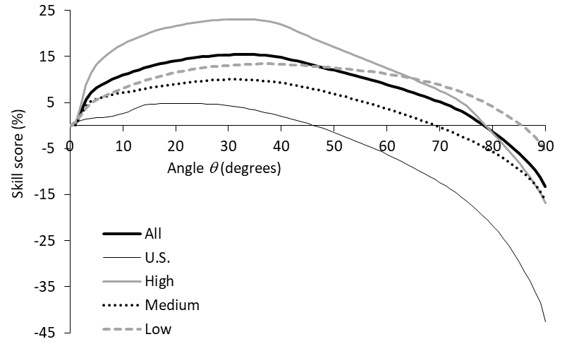
Figure 11: 95% interval skill score for the out-of-sample period for angular averaging at different angles. Higher values of the skill score are better.

5.5 Optimized Values of the Angle

In practice, the angle $\theta$ would need to be estimated. For angular averaging and angular weighted combining, Figure 12 summarizes the values of the angle optimized for these two methods using the in-sample MQS at the 74 forecast origins for the 52 series. The left extreme of the figure shows that angles close to the horizontal ($\theta=0^{\textrm{o}}$) were quite often found to be optimal. However, the right end of the figure shows that the optimized angle was more frequently found to be closer to vertical ($\theta=90^{\textrm{o}}$), with angles between about $70^{\textrm{o}}$ and $90^{\textrm{o}}$ often obtained.

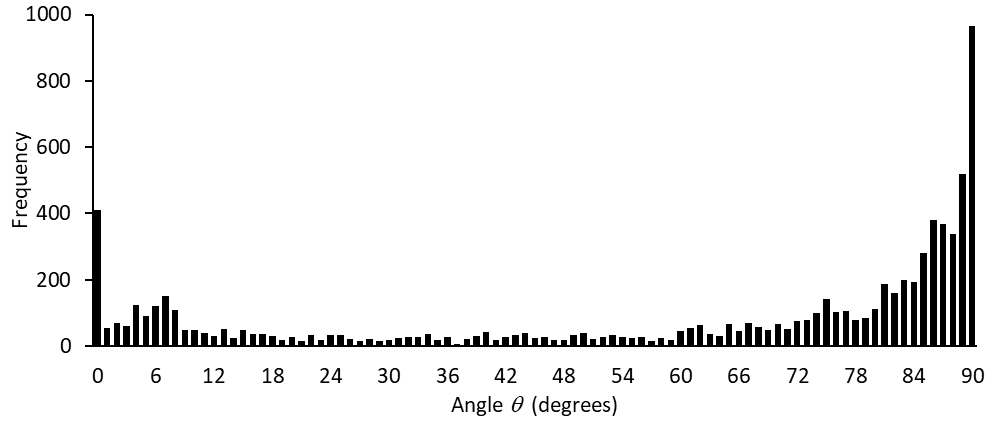
Figure 12: For angular averaging and angular weighted combining, histogram of the angle $\theta$ optimized for the 52 series at the 74 forecast origins.

5.6 Comparing Horizontal, Vertical and Angular Combining using the MQS

In this section, we evaluate the out-of-sample performance of angular combining with optimized angle by comparing it with horizontal and vertical combining, as well as horizontal/vertical switching. Table 1 summarizes the MQS results. The first five columns of values provide the MQS for each of the five categories of the time series considered in Figures 10 and 11. Lower values of the MQS are better. The final five columns of Table 1 present the corresponding skill scores. In each column, bold highlights the best approach to averaging and the best approach to weighted combining. Looking at the averaging approaches in the first four rows, we see that horizontal averaging was the most accurate for the U.S. national level series and the poorest for the other four categories. The horizontal/vertical switching method performed well for the U.S. national level series because it selected horizontal averaging for all forecast origins. For the other four categories, the skill scores show that the switching method was not able to outperform vertical averaging. For these four categories, angular averaging was a little more accurate than vertical averaging. For weighted combining, we again see horizontal combining performing well only for the U.S. national level series, with angular combining again a little better than vertical combining overall. We also note that each form of weighted combining outperforms the corresponding form of averaging.

Table 1: MQS for the out-of-sample period for the three forms of averaging and horizontal/vertical switching.

			MQS				MQS skill score (%)
	All	U.S.	High	Medium	Low		All	U.S.	High	Medium	Low
Averaging
Horizontal	55.5	897.3	80.1	28.5	8.5		0.0	0.0	0.0	0.0	0.0
Vertical	52.6	949.1	69.2	27.7	8.2		4.7	-5.8	7.9	2.2	4.6
Horizontal/vertical switching	51.9	897.3	69.8	27.9	8.2		3.8	0.0	6.8	1.4	3.4
Angular	51.5	903.3	68.5	27.5	8.2		5.5	-0.7	8.9	3.1	4.8
Weighted combining
Horizontal	52.5	834.1	75.2	28.0	8.2		3.8	7.0	6.0	2.4	2.7
Vertical	50.5	884.5	67.1	27.3	8.1		6.6	1.4	10.6	3.6	5.8
Horizontal/vertical switching	49.7	834.1	67.3	27.6	8.1		6.2	7.0	10.8	3.1	4.6
Angular	49.4	839.4	66.3	27.3	8.1		7.3	6.5	12.0	4.2	5.6

Note: The unit of the score is deaths. Lower values of the score and higher values of the skill score are better. The skill score uses horizontal averaging as benchmark. Bold indicates the best method in each column within the averaging block and within the weighted combining block.

In Figure 13, for each of the 52 series, we present the skill scores for horizontal, vertical and angular averaging, as well as horizontal/vertical switching. The series are ordered according to cumulative mortality at the end of the dataset. The skill scores are all zero for horizontal averaging, as this was used as the benchmark in the skill score calculation. For angular averaging, the skill scores are generally positive, and sometimes high, reflecting clear outperformance of horizontal averaging. Comparing angular and vertical averaging, the figure shows that there are a few series for which vertical was slightly better than angular averaging, and there were about a dozen series for which angular averaging was noticeably more accurate, with these series being those for which horizontal averaging outperformed vertical averaging. It can also be seen from Figure 13 that, overall, angular averaging performed better than horizontal/vertical switching. Looking in more detail, we found that this was the case for 38 out of the 52 series. In the analogous plot for weighted combining, the relative performances of horizontal, vertical and angular combining, and horizontal/vertical switching, were similar to Figure 13. In the next section, we look more deeply into the relative merits of the methods by evaluating accuracy for different regions of the distribution.

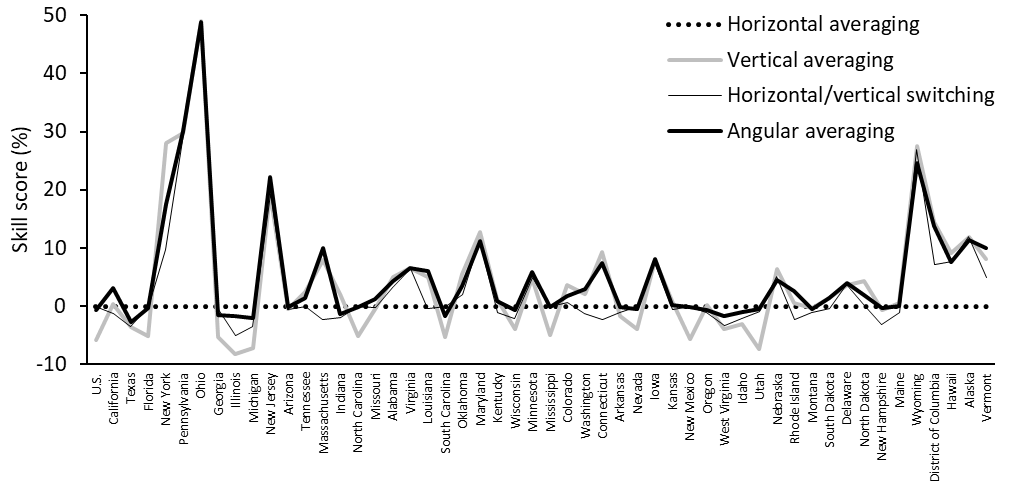
Figure 13: MQS skill score for the out-of-sample period for the three forms of averaging and horizontal/vertical switching. Higher values of the skill score are better.

5.7 Comparing Horizontal, Vertical and Angular Combining using Interval Scores

Table 2 reports the results for the 95% interval score and skill score. Interestingly, in comparison with the MQS results of Table 1, the results in Table 2 show clearer superiority of angular combining over horizontal and vertical combining, as well as horizontal/vertical switching. This indicates that angular combining is particularly beneficial for estimating the tails of the mortality distributions. It is also interesting to see horizontal outperforming vertical combining in terms of the 95% interval, while the opposite was true when the whole distributional forecast was evaluated in Table 1.

Table 2: 95% interval score for the out-of-sample period for the three forms of averaging and horizontal/vertical switching.

	Interval score						Interval skill score (%)
	All	U.S.	High	Medium	Low		All	U.S.	High	Medium	Low
Averaging
Horizontal	779.6	9250.7	1249.1	472.4	119.0		0.0	0.0	0.0	0.0	0.0
Vertical	895.3	13197.6	1347.8	496.9	117.5		-13.2	-42.7	-16.8	-16.1	-5.4
Horizontal/vertical switching	774.5	9250.7	1236.8	472.9	115.3		-3.5	0.0	-3.4	-4.4	-3.0
Angular	745.3	10017.6	1130.1	446.3	114.2		3.3	-8.3	8.1	3.2	-1.1
Weighted combining
Horizontal	716.0	8749.4	1111.0	457.8	106.6		8.3	5.4	12.0	5.1	7.8
Vertical	787.9	12228.1	1113.2	466.4	111.2		-1.2	-32.2	1.7	-6.4	2.3
Horizontal/vertical switching	695.5	8749.4	1041.8	463.5	107.4		6.5	5.4	11.8	0.6	6.9
Angular	678.3	9385.7	972.2	443.9	106.6		10.7	-1.5	19.0	5.3	7.7

Note: The unit of the score is deaths. Lower values of the score and higher values of the skill score are better. The skill score uses horizontal averaging as benchmark. Bold indicates the best method in each column within the averaging block and within the weighted combining block.

For each of the 52 series, Figure 14 plots the 95% interval skill scores for horizontal, vertical and angular averaging, as well as horizontal/vertical switching. By contrast with the MQS results in Figure 13, Figure 14 shows several series for which angular averaging comfortably outperforms both vertical and horizontal averaging. There are some series for which angular averaging is outperformed by horizontal averaging, but very few series for which vertical averaging is more accurate than angular averaging. We obtained similar insight from the analogous figure for the 95% interval skill scores for weighted combining.

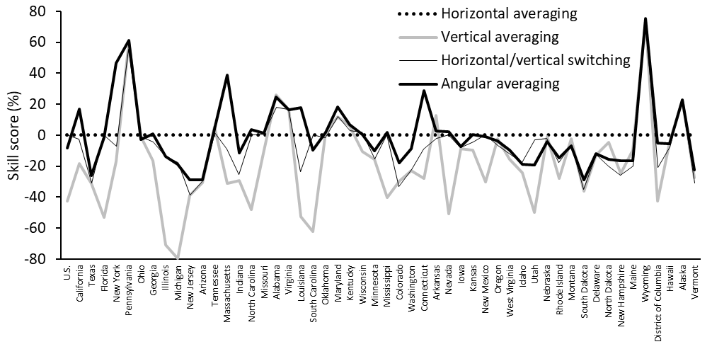
Figure 14: 95% interval skill score for the out-of-sample period for the three forms of averaging and horizontal/vertical switching. Higher values of the skill score are better.

Table 3 presents the results for the 50% intervals. For both averaging and weighted combining, the skill scores for vertical combining are generally a little better than angular combining. In Figure 15, where the skill scores are shown for each of the 52 series, we see vertical and angular averaging generally outperforming horizontal averaging.

We also computed the interval score for $(1-\alpha)\times 100\%$ intervals constructed from other pairs of the 23 quantiles. For $\alpha\leq 30\%$, we found that angular combining was comfortably more accurate than vertical combining (as in Table 2 for the 95% intervals). For $\alpha\geq 50\%$, vertical outperformed angular combining by a relatively small amount (as in Table 3 for the 50% intervals). It is worth noting that the MQS can be expressed as a weighted sum of all these interval scores (plus the absolute deviation between observation and median), where the weight on the $(1-\alpha)\times 100\%$ interval score is proportional to $\alpha$ (Bracher et al., 2021a ). This explains why vertical combining was able to be competitive in terms of the MQS in Table 1, even though it was comfortably outperformed by angular combining for the intervals corresponding to $\alpha\leq 30\%$.

Table 3: 50% interval score for the out-of-sample period for the three forms of averaging and horizontal/vertical switching.

	Interval score						Interval skill score (%)
	All	U.S.	High	Medium	Low		All	U.S.	High	Medium	Low
Averaging
Horizontal	270.1	4524.5	380.9	137.5	41.6		0.0	0.0	0.0	0.0	0.0
Vertical	253.5	4619.6	331.1	132.8	39.7		5.5	-2.1	7.8	2.9	6.1
Horizontal/vertical switching	254.0	4524.5	335.8	134.8	40.2		3.8	0.0	5.7	1.6	4.3
Angular	253.4	4557.8	333.5	133.5	40.0		4.8	-0.7	6.7	2.6	5.3
Weighted combining
Horizontal	255.5	4168.1	360.6	135.1	40.8		3.2	7.9	5.1	2.2	2.1
Vertical	244.6	4310.1	323.6	131.6	39.5		6.7	4.7	9.6	4.1	6.6
Horizontal/vertical switching	243.2	4168.1	325.3	133.4	40.0		5.6	7.9	8.9	2.9	4.5
Angular	242.7	4183.9	324.1	132.4	39.8		6.3	7.5	9.4	3.8	5.5

Note: The unit of the score is deaths. Lower values of the score and higher values of the skill score are better. The skill score uses horizontal averaging as benchmark. Bold indicates the best method in each column within the averaging block and within the weighted combining block.

Figure 15: 50% interval skill score for the out-of-sample period for the three forms of averaging and horizontal/vertical switching. Higher values of the skill score are better.

5.8 Comparing Horizontal, Vertical and Angular Combining using Calibration

Table 4 presents the unconditional calibration of 95% and 50% intervals obtained from the distributional forecasts of the various methods. The ideal values are 95% and 50%, respectively. For the 95% intervals, the intervals from horizontal combining tended to be too narrow, while the intervals from vertical combining tended to be a too wide, with this being particularly the case for the U.S. national series. The best results overall correspond to angular combining. Turning to the 50% intervals, we see that, by contrast with the interval score results in Table 3, the calibration results show horizontal combining performing better than vertical combining, with the intervals resulting from vertical combining tending to be too wide, with this, again, being particularly apparent for the U.S. national series. For the 50% intervals, angular combining performed reasonably well, although not quite as well overall as horizontal combining.

Table 4: Interval calibration (%) for the out-of-sample period for the three forms of averaging and horizontal/vertical switching.

	95% interval						50% interval
	All	U.S.	High	Medium	Low		All	U.S.	High	Medium	Low
Averaging
Horizontal	88.3	93.5	89.6	89.9	85.2		51.1	57.9	52.3	51.7	48.9
Vertical	96.4	99.0	97.4	97.1	94.7		62.1	67.9	65.4	64.2	56.4
Horizontal/vertical switching	93.1	93.5	93.8	94.0	91.4		56.6	57.9	58.3	57.6	53.7
Angular	94.1	93.5	95.0	95.0	92.2		53.5	57.2	56.4	54.4	49.5
Weighted combining
Horizontal	89.3	96.6	90.3	91.1	86.1		51.8	59.3	53.6	53.2	48.2
Vertical	96.3	99.0	97.3	97.0	94.3		60.8	71.0	64.2	63.1	54.4
Horizontal/vertical switching	92.9	96.6	93.8	93.9	90.9		55.9	59.3	58.2	57.6	51.7
Angular	93.6	95.9	94.4	94.8	91.4		53.3	58.6	56.1	54.9	48.6

Note: The values are the percentage of observations falling within the intervals. For 95% and 50% intervals, the ideal values are 95% and 50%, respectively. Bold indicates the best method in each column within the averaging block and within the weighted combining block.

To provide more detail regarding calibration, Figure 16 presents reliability diagrams for the five categories of series for the horizontal, vertical and angular averaging. Each diagram conveys the unconditional calibration of the 23 quantiles, with the ideal indicated by the diagonal dotted line in each plot (see Hora, 2004). The reliability diagram is a cumulative version of the probability integral transform (Pinson et al., 2010). For vertical averaging, the plots show that too few of the out-of-sample observations exceeded the quantiles in the lower half of the distributional forecasts. This is consistent with the finding in Table 4 that the interval forecasts from this method were, on average, too wide. Figure 16 shows that horizontal and angular averaging produced better calibration than vertical averaging for the lower quantiles, while all three methods performed well for quantiles in the upper half of the distributional forecasts.

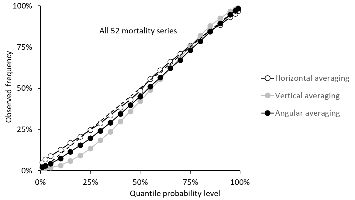
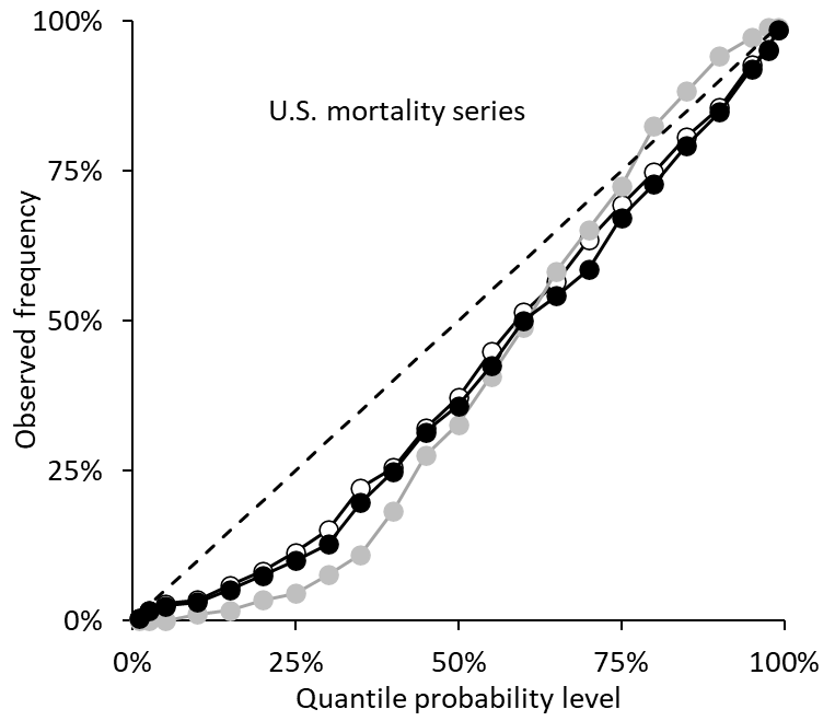
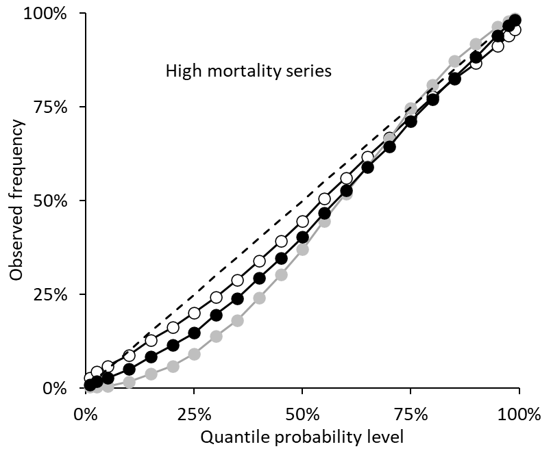
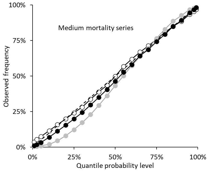
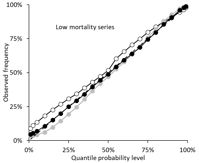
Figure 16: Reliability diagrams for the out-of-sample period for horizontal, vertical and angular averaging.

5.9 Evaluating Other Methods using the MQS

Although our aim in this paper is to introduce angular combining as an alternative to horizontal and vertical combining, it is also interesting to see how other methods from the literature perform for the mortality dataset. Table 5 reports the results for the methods listed below. Method parameters were optimized by minimizing the in-sample MQS at each of the 74 forecast origins for each of the 52 series.

Median combining – This is the simple method considered by Hora et al., (2013).

Beta-transformed linear pool – Gneiting and Ranjan, (2013) use the beta distribution to transform the distributional forecast of a linear pool (i.e., vertical combination), which we specified as the average and as a weighted combination with weights defined as in the weighted combining methods of Table 1. The implementation involved the optimization of the two parameters of the beta distribution. We were unable to implement the generalized linear combinations of Gneiting and Ranjan, (2013), discussed in Section 3.3, because the link functions that they propose have domains that do not include 0 and 1, which is needed for application to our dataset of individual distributional forecasts.

Trimming – We implemented the trimming approach of Jose et al., (2014) that bases trimming on the mean of each distributional forecast. Exterior trimming involves averaging the distributional forecasts that remain after removing a percentage of the individual distributional forecasts with lowest and highest mean. Interior trimming involves averaging the distributional forecasts that were among a percentage of those with lowest and highest mean. We implemented these methods with vertical, horizontal and angular averaging. Each form of trimming required the optimization of the trimming percentage.

Recalibration – Han and Budescu, (2022) recalibrate a distributional forecast by transforming the probabilities corresponding to predefined bins. We applied the recalibration to the three averaging and three weighted combining methods in Table 1. For each distribution, we defined the bins as the 24 intervals bounded by the quantiles corresponding to the 23 probability levels of focus in the COVID-19 Forecast Hub, and the lower and upper bounds of each distribution. The method involved optimizing one parameter.

In Table 5, underlining indicates a value that is better than the corresponding value for any other method in Tables 1 and 5. The beta-transformed linear pool performed notably well when the weighted linear pool was applied to the distributional forecasts of the U.S. national series, but apart from this, was uncompetitive with the better of the other methods. The best trimming method was exterior trimming with vertical averaging. In terms of the skill score averaged over all 52 series, this method was better than any other method in Tables 1 and 5, slightly outperforming angular weighted combining in Table 1. Comparing the results for this trimming method in Table 5 with the results for vertical averaging in Table 1, we see that applying exterior trimming to vertical averaging was particularly beneficial for the U.S. national series. This is not surprising, in view of the calibration results in Table 4, which showed that vertical averaging produced distributions that were, on average, overly dispersed. Recalibration also performed well, when applied to the distributional forecasts produced by vertical averaging or vertical weighted combining.

Table 5: MQS for the out-of-sample period for a variety of combining and recalibration methods.

	MQS						MQS skill score (%)
	All	U.S.	High	Medium	Low		All	U.S.	High	Medium	Low
Simple benchmark
Median	51.5	914.1	68.1	27.6	8.1		6.6	-1.9	10.6	3.2	6.3
Beta-transformed linear pool
Averaging	53.2	893.3	73.6	28.2	8.5		3.1	0.4	6.9	0.4	2.0
Weighted combining	51.7	825.8	72.5	28.5	8.5		2.6	8.0	6.7	-0.4	1.2
Exterior trimming
Horizontal	55.0	897.0	79.3	27.8	8.2		3.6	0.0	3.5	2.5	5.1
Vertical	50.7	896.4	67.0	27.3	8.1		7.4	0.1	11.9	3.9	6.6
Angular	51.4	901.0	68.6	27.6	8.1		6.2	-0.4	9.8	3.1	5.8
Interior trimming
Horizontal	61.5	897.4	98.0	28.8	8.5		-2.5	0.0	-5.3	-1.3	-1.1
Vertical	53.7	951.0	72.3	27.7	8.2		3.9	-6.0	6.1	1.8	4.3
Angular	61.1	905.3	97.6	27.8	8.3		1.1	-0.9	-2.2	1.9	3.6
Recalibration of averaging
Horizontal	56.3	904.0	81.8	28.8	8.5		-0.9	-0.8	-2.1	-0.9	0.2
Vertical	51.4	919.2	67.8	27.3	8.1		7.1	-2.4	11.0	4.1	6.7
Angular	54.1	933.8	72.2	29.7	8.7		-0.9	-4.1	4.9	-4.5	-3.3
Recalibration of weighted combining
Horizontal	54.0	849.1	78.3	28.5	8.4		1.3	5.4	2.7	0.4	0.5
Vertical	49.8	852.3	66.4	27.7	8.1		7.1	5.0	12.4	3.2	5.7
Angular	52.6	891.8	70.2	29.5	8.9		-0.2	0.6	7.6	-3.3	-5.5

Note: The unit of the score is deaths. Lower values of the score and higher values of the skill score are better. The skill score uses horizontal averaging from Table 1 as benchmark. Bold indicates the best method in each column. Underlining indicates a result that is better than any other in the same column of Tables 1 and 5.

As angular combining conceptually lies between horizontal and vertical combining, it could be suggested that angular combining is perhaps equivalent to a secondary weighted combination of the distributional forecasts produced by horizontal and vertical combining, with the weights related to the angle $\theta$. When $\theta=0^{\textrm{o}}$, the weight on the horizontally combined forecast would equal 1, and when $\theta=90^{\textrm{o}}$, the weight on the vertically combined forecast would be 1. However, the question would then be whether this secondary weighted combination should be performed horizontally or vertically. We implemented both possibilities, with the weights for the secondary combination estimated by minimizing the sum of in-sample MQS. The first two rows of values in Table 6 are the out-of-sample MQS results for horizontal and vertical secondary weighted combinations of the two distributional forecasts resulting from horizontal and vertical averaging of the individual distributional forecasts. These results differ from, and are poorer than, the results for angular averaging in Table 1. In Table 6, the third and fourth rows of values are the results for secondary horizontal and vertical weighted combining of the two distributional forecasts produced by horizontal and vertical performance-weighted combining of the individual distributional forecasts. These results differ from, and are not as good as, the results for angular weighted combining in Table 1.

Table 6: MQS for the out-of-sample period for combinations of combinations.

	MQS						MQS skill score (%)
	All	U.S.	High	Medium	Low		All	U.S.	High	Medium	Low
Combining horizontal & vertical averages
Horizontal secondary weighted combining	51.9	901.9	69.9	27.7	8.2		4.4	-0.5	6.7	2.5	4.3
Vertical secondary weighted combining	54.4	914.0	76.3	28.1	8.2		2.4	-1.9	2.2	0.8	4.4
Combining horizontal & vertical weighted combinations
Horizontal secondary weighted combining	49.7	839.8	67.3	27.4	8.1		6.6	6.4	10.6	4.1	4.9
Vertical secondary weighted combining	52.0	846.9	73.6	27.4	8.1		4.9	5.6	5.8	3.9	5.0

Note: The unit of the score is deaths. Lower values of the score and higher values of the skill score are better. The skill score uses horizontal averaging from Table 1 as benchmark. Bold indicates the best method in each column.

6 Summary and Concluding Remarks

In the literature on distributional forecasting, the question has been posed as to whether it is better to average horizontally or vertically. We have viewed this as an empirical question, and have extended the debate by proposing that combining can be performed at an angle, leading to a method that lies between the extremes of horizontal and vertical combining. Although our suggestion of angular combining is motivated by empirical pragmatism, we feel the approach is interesting conceptually, and we have endeavored to convey this with graphical illustrations for simple examples involving Gaussian distributions. We extended the theoretical results of Lichtendahl et al., (2013) to obtain several interesting results for angular averaging. Firstly, like vertical and horizontal averaging, angular averaging produces distributional forecasts for which the mean is the average of the means of the individual distributional forecasts in the combination. Secondly, angular averaging produces a distribution with lower variance than vertical averaging, and, under certain assumptions, greater variance than horizontal averaging. Thirdly, as with vertical and horizontal averaging, the CRPS for angular averaging is no worse than the average score of the distributional forecasts in the combination. Fourthly, the median combination, which gives the same distribution when performed horizontally or vertically, also delivers the same distribution when performed at an angle.

Our empirical study used forecasts produced by multiple forecasting teams of weekly COVID-19 mortality. We illustrated our proposals by implementing angular averaging and performance-weighted angular combining. The out-of-sample results were encouraging, with the score for distributional forecast accuracy showing angular combining performing as well as the better of horizontal and vertical combining for each mortality series considered. Angular combining performed particularly well in terms of the accuracy of the tails of the distributional forecasts. The method was also found to be competitive when compared against a variety of combining and recalibration methods from the literature.

In terms of future research, we would welcome further empirical studies to gauge the usefulness of angular combining for different applications. In this paper, we have worked with a dataset consisting of distributional forecasts from between approximately 10 to 30 forecasting teams. The scope for different forms of performance-based weighted combining was limited by historical accuracy not being available for the same past periods for all teams. It would be interesting to evaluate the potential for angular combining when there is a relatively small number of distributional forecasts to be combined, with comparable past accuracy available for each. In our empirical analysis, we used parameter estimation samples of between 10 and 84 periods. It would be useful to evaluate the performance of angular combining for applications where larger sample sizes are available to estimate the angle $\theta$.

Appendix: Proofs of Main Results

Throughout the proofs, we make a standard assumption that all distributions have finite mean and variance. The vertical average can be viewed as a mixture distribution, and it is well-known that the moments of a mixture distribution equals the sum of the moments of its components. This widely-known result will not be explicitly mentioned in our proofs. Notice that the inverse transformation of $h_{\theta}$ defined in (7) is simply $h_{-\theta}$, hence $F=h_{-\theta}(h_{\theta}(F))$ for any CDF $F$. The angular average $F_{A,\theta}$ can be written as $h_{-\theta}\left(\frac{1}{k}\sum_{i=1}^{k}h_{\theta}(F_{i})\right)$ where $\frac{1}{k}\sum_{i=1}^{k}h_{\theta}(F_{i})$ denotes the vertical average of $h_{\theta}(F_{i})$. We first prove Lemma 3.1,

Proof 6.1

Proof of Proposition 3.1 Note that for each $i$, based on the line $y=\tan\theta(x-c)$, the parameterization of the $F_{i}$ yields $F_{i}\left(x_{i}\left(c\right)\right)=-\tan\theta\left(x_{i}(c)-c\right)$. Utilizing the chain rule, we have $\frac{dx_{i}(c)}{dc}=\frac{d\left(-F\left(x_{i}\left(c\right)\right)/\tan\theta+c\right)}{dc}=-f_{i}\left(x_{i}(c)\right)\frac{dx_{i}\left(c\right)}{dc}/\tan\theta+1$. Solving this equation, we obtain that $\frac{dx_{i}(c)}{dc}=\frac{\tan\theta}{f_{i}\left(x_{i}(c)\right)+\tan\theta}$. Therefore, the PDF $f_{A,\theta}$ for angular averaging can be obtained via the chain rule,

$$f_{A,\theta}\left(\frac{1}{k}\sum_{i=1}^{k}x_{i}(c)\right) =\frac{d\left(\frac{1}{k}\sum_{i=1}^{k}F_{i}(x_{i}(c))\right)}{dc}\frac{dc}{d\left(\frac{1}{k}\sum_{i=1}^{k}x_{i}(c)\right)}$$

$$=\left(\sum_{i=1}^{k}f_{i}\left(x_{i}(c)\right)\frac{dx_{i}\left(c\right)}{dc}\right)\Bigg{/}\left(\sum_{i=1}^{k}\frac{dx_{i}(c)}{dc}\right)$$

$$=\left(\sum_{i=1}^{k}\frac{f_{i}\left(x_{i}(c)\right)\tan\theta}{f_{i}\left(x_{i}(c)\right)+\tan\theta}\right)\Bigg{/}\left(\sum_{i=1}^{k}\frac{\tan\theta}{f_{i}\left(x_{i}(c)\right)+\tan\theta}\right)$$

$$=\left(\sum_{i=1}^{k}\frac{f_{i}\left(x_{i}(c)\right)}{f_{i}\left(x_{i}(c)\right)+\tan\theta}\right)\Bigg{/}\left(\sum_{i=1}^{k}\frac{1}{f_{i}\left(x_{i}(c)\right)+\tan\theta}\right)$$

Before showing the rest of the proofs, we first present Lemma 6.2, which is a technical lemma.

Lemma 6.2

Let $F$ be any CDF, we have the following results,

i) the mean of the distribution with CDF $h_{\theta}(F)$ equals $\mathbb{E}_{X\sim F}\left[X\right]+\frac{1}{2\tan\theta}$.

ii) the expectation of $X^{2}$ for the distribution with CDF $h_{\theta}(F)$ is $\mathbb{\mathbb{E}}_{X\sim F}\left[X^{2}\right]+\frac{1}{3\tan^{2}\theta}+\frac{1}{\tan\theta}\intop_{-\infty}^{\infty}xdF(x)^{2}$.

Proof 6.3

Proof of Lemma 6.2 i) The statement can be proved as follows,

$$\mathbb{E}_{X\sim h_{\theta}(F)}\left[X\right] =\intop_{0}^{1}h_{\theta}(F)^{-1}(\alpha)d\alpha=\intop_{0}^{1}\left(F^{-1}(\alpha)+\frac{\alpha}{\tan\theta}\right)d\alpha=\mathbb{E}_{X\sim F}\left[X\right]+\frac{1}{2\tan\theta}.$$

ii) The statement can be proved as follows,

$$\mathbb{E}_{X\sim h_{\theta}(F)}\left[X^{2}\right] =\intop_{0}^{1}\left(h_{\theta}(F)^{-1}(\alpha)\right)^{2}d\alpha$$

$$=\intop_{0}^{1}\left(F^{-1}(\alpha)+\frac{\alpha}{\tan\theta}\right)^{2}d\alpha$$

$$=\intop_{0}^{1}\left\{\left(F^{-1}(\alpha)\right)^{2}+\frac{\alpha^{2}}{\tan^{2}\theta}+2F^{-1}(\alpha)\frac{\alpha}{\tan\theta}\right\}d\alpha$$

$$=\mathbb{\mathbb{E}}_{X\sim F}\left[X^{2}\right]+\frac{1}{3\tan^{2}\theta}+\frac{1}{\tan\theta}\intop_{0}^{1}2F^{-1}(\alpha)\alpha d\alpha$$

$$=\mathbb{\mathbb{E}}_{X\sim F}\left[X^{2}\right]+\frac{1}{3\tan^{2}\theta}+\frac{1}{\tan\theta}\intop_{-\infty}^{\infty}2xF(x)dF(x)$$

$$=\mathbb{\mathbb{E}}_{X\sim F}\left[X^{2}\right]+\frac{1}{3\tan^{2}\theta}+\frac{1}{\tan\theta}\intop_{-\infty}^{\infty}xdF(x)^{2}.$$

For the third last equality, the integral $\intop_{0}^{1}2F^{-1}(\alpha)\alpha d\alpha$ is well-defined by the dominated convergence theorem and the inequality $\big{|}F^{-1}(\alpha)\alpha\big{|}\leq\big{|}F^{-1}(\alpha)\big{|}$ for $\alpha\in(0,1)$, and the third term in the penultimate line is obtained by making use of the change of variable $F(x)=\alpha$.

Proof 6.4

Proof of Proposition 4.1 By (8) in Section 3.3, we have $F_{A,\theta}=h_{-\theta}\left(\frac{1}{k}\sum_{i=1}^{k}h_{\theta}(F_{i})\right)$. Firstly, by Lemma 6.2(i), $\mathbb{E}_{X\sim\frac{1}{k}\sum_{i=1}^{k}h_{\theta}(F_{i})}\left[X\right]=\frac{1}{k}\sum_{i=1}^{k}\mathbb{E}_{h_{\theta}(F_{i})}\left[X\right]=\frac{1}{k}\sum_{i=1}^{k}\left(\mathbb{E}_{X\sim F_{i}}\left[X\right]+\frac{1}{2\tan\theta}\right).$ Next, by applying Lemma 6.2(i) to $h_{-\theta}$, we get $\mathbb{E}_{X\sim F_{A,\theta}}\left[X\right]=\mathbb{E}_{X\sim h_{-\theta}\left(\frac{1}{k}\sum_{i=1}^{k}h_{\theta}(F_{i})\right)}\left[X\right]=\mathbb{E}_{X\sim\frac{1}{k}\sum_{i=1}^{k}h_{\theta}(F_{i})}\left[X\right]-\frac{1}{2\tan\theta}=\frac{1}{k}\sum_{i=1}^{k}\mathbb{E}_{X\sim F_{i}}\left[X\right].$ Hence, the mean of $F_{A,\theta}$ is identical to the average of the means of the individual distributions $F_{i}$.

Proof 6.5

Proof of Theorem 4.2 By Proposition 4.1, we have $\mathbb{E}_{X\sim F_{A,\theta}}\left[X\right]=\mathbb{E}_{X\sim F_{V}}\left[X\right]$. Therefore, we only need to show that $\mathbb{E}_{X\sim F_{A,\theta}}\left[X^{2}\right]-\mathbb{E}_{X\sim F_{V}}\left[X^{2}\right]\leq 0$. Using Lemma 6.2(ii), we first compute $\mathbb{E}_{X\sim\frac{1}{k}\sum_{i=1}^{k}h_{\theta}(F_{i})}\left[X^{2}\right]$ as follows,

$$\mathbb{E}_{X\sim\frac{1}{k}\sum_{i=1}^{k}h_{\theta}(F_{i})}\left[X^{2}\right]=\frac{1}{k}\sum_{i=1}^{k}\mathbb{E}_{h_{\theta}(F_{i})}\left[X^{2}\right]=\frac{1}{k}\sum_{i=1}^{k}\left(\mathbb{\mathbb{E}}_{X\sim F_{i}}\left[X^{2}\right]+\frac{1}{3\tan^{2}\theta}+\frac{1}{\tan\theta}\intop_{-\infty}^{\infty}xdF_{i}(x)^{2}\right)$$

Next, we show $\mathbb{E}_{X\sim F_{A,\theta}}\left[X^{2}\right]-\mathbb{E}_{X\sim F_{V}}\left[X^{2}\right]\leq 0$,

$$\mathbb{E}_{X\sim F_{A,\theta}}\left[X^{2}\right]-\mathbb{E}_{X\sim F_{V}}\left[X^{2}\right]$$

$$=\mathbb{E}_{X\sim h_{-\theta}\left(\frac{1}{k}\sum_{i=1}^{k}h_{\theta}(F_{i})\right)}\left[X^{2}\right]-\frac{1}{k}\sum_{i=1}^{k}\mathbb{\mathbb{E}}_{X\sim F_{i}}\left[X^{2}\right]$$

$$=\mathbb{E}_{X\sim h_{-\theta}\left(\frac{1}{k}\sum_{i=1}^{k}h_{\theta}(F_{i})\right)}\left[X^{2}\right]-\frac{1}{k}\sum_{i=1}^{k}\mathbb{\mathbb{E}}_{X\sim h_{-\theta}\left(h_{\theta}(F_{i})\right)}\left[X^{2}\right]$$

$$=\frac{1}{k}\sum_{i=1}^{k}\mathbb{\mathbb{E}}_{X\sim h_{\theta}(F_{i})}\left[X^{2}\right]+\frac{1}{3\tan^{2}\theta}-\frac{1}{\tan\theta}\intop_{-\infty}^{\infty}xd\left(\frac{1}{k}\sum_{i=1}^{k}h_{\theta}(F_{i})(x)\right)^{2}$$

$$\quad-\frac{1}{k}\sum_{i=1}^{k}\mathbb{\mathbb{E}}_{X\sim h_{\theta}(F_{i})}\left[X^{2}\right]-\frac{1}{3\tan^{2}\theta}+\frac{1}{\tan\theta}\frac{1}{k}\sum_{i=1}^{k}\intop_{-\infty}^{\infty}xd\left(h_{\theta}(F_{i})(x)\right)^{2}$$

$$=\frac{1}{\tan\theta}\left\{\intop_{-\infty}^{\infty}xd\left(\frac{1}{k}\sum_{i=1}^{k}\left(h_{\theta}(F_{i})(x)\right)^{2}-\left(\frac{1}{k}\sum_{i=1}^{k}h_{\theta}(F_{i})(x)\right)^{2}\right)\right\}$$

$$=\frac{1}{\tan\theta}\left[x\left(\frac{1}{k}\sum_{i=1}^{k}h_{\theta}(F_{i})(x)^{2}-\left(\frac{1}{k}\sum_{i=1}^{k}h_{\theta}(F_{i})(x)\right)^{2}\right)\right]_{-\infty}^{\infty}$$

$$\quad-\frac{1}{\tan\theta}\intop_{-\infty}^{\infty}\left\{\frac{1}{k}\sum_{i=1}^{k}h_{\theta}(F_{i})(x)^{2}-\left(\frac{1}{k}\sum_{i=1}^{k}h_{\theta}(F_{i})(x)\right)^{2}\right\}dx$$

$$=\frac{-1}{\tan\theta}\intop_{-\infty}^{\infty}\left\{\frac{1}{k}\sum_{i=1}^{k}h_{\theta}(F_{i})(x)^{2}-\left(\frac{1}{k}\sum_{i=1}^{k}h_{\theta}(F_{i})(x)\right)^{2}\right\}dx$$

$$\leq 0$$

The second equality uses the relation that $F_{i}=h_{-\theta}\left(h_{\theta}(F_{i})\right)$, the third equality uses Lemma 6.2(ii), the penultimate equality stems from the integration by parts, and the final equality uses the result that $x\left(\frac{1}{k}\sum_{i=1}^{k}h_{\theta}(F_{i})(x)^{2}-\left(\frac{1}{k}\sum_{i=1}^{k}h_{\theta}(F_{i})(x)\right)^{2}\right)$ tends to 0 as $x$ tends to $\pm\infty$. To see this, for any distribution with CDF $F$ and PDF $f$, when $x<0$, $\big{|}xF(x)^{2}\big{|}\leq\big{|}xF(x)\big{|}=-x\intop_{-\infty}^{x}f(s)d(s)\leq\intop_{-\infty}^{x}|s|f(s)d(s)$, which tends to 0 as $x\rightarrow-\infty$, under our assumption that the mean $\mathbb{E}_{X\sim F}\left[X\right]$ is finite. Hence $x\left(\frac{1}{k}\sum_{i=1}^{k}h_{\theta}(F_{i})(x)^{2}-\left(\frac{1}{k}\sum_{i=1}^{k}h_{\theta}(F_{i})(x)\right)^{2}\right)=x\frac{1}{k}\sum_{i=1}^{k}h_{\theta}(F_{i})(x)^{2}-x\left(\frac{1}{k}\sum_{i=1}^{k}h_{\theta}(F_{i})(x)\right)^{2}$ goes to 0 when $x\rightarrow-\infty$. Similarly, $\big{|}x\left(1-F(x)^{2}\right)\big{|}$ tends to 0 as $x\rightarrow\infty$ for any CDF $F$, so $x\left(\frac{1}{k}\sum_{i=1}^{k}h_{\theta}(F_{i})(x)^{2}-\left(\frac{1}{k}\sum_{i=1}^{k}h_{\theta}(F_{i})(x)\right)^{2}\right)=x\bigg{\{}1-\frac{1}{k}\sum_{i=1}^{k}h_{\theta}(F_{i})(x)^{2}\bigg{\}}-x\bigg{\{}1-\left(\frac{1}{k}\sum_{i=1}^{k}h_{\theta}(F_{i})(x)\right)^{2}\bigg{\}}$ goes to 0 when $x\rightarrow\infty$ . The final inequality is due to the standard arithmetic mean - quadratic mean inequality.

Proof 6.6

Proof of Lemma 4.3 Without loss of generality, let $f_{0}$ be a symmetric and unimodal PDF about 0 and let $F_{0}$ denote its CDF. Let $F_{1}(x)=F_{0}(x+\mu)$ and $F_{2}(x)=F_{0}(x-\mu)$, for some $\mu>0$, denote the two individual distributions that are being averaged. By Proposition 4.1, the common mean of $F_{A,\theta}$, $F_{V}$, and $F_{H}$ is 0.

i) We show that, for angular averaging, the PDF $f_{A,\theta}$ is symmetric about 0. It is sufficient to show that $F_{A,\theta}\left(-z\right)=1-F_{A,\theta}\left(z\right)$ for $z<0$. By the definition of angular averaging and the fact that $F_{1}$ is positioned on the left-hand side of $F_{2}$, there exists $t>0$ such that $F_{A,\theta}(z)=\frac{1}{2}\left(F_{1}(z-t)+F_{2}(z+t)\right)=\frac{1}{2}\left(F_{0}(z-t+\mu)+F_{0}(z+t-\mu)\right)$, where $\left(z-t,F_{0}(z-t+\mu)\right)$ and $\left(z+t,F_{0}(z+t-\mu)\right)$ are on the line $y=-\tan\theta(x-c)$ for some $c$, which is equivalent to stating that the gradient of the straight line between these two points $\frac{1}{2t}\left(F_{0}(z+t-\mu)-F_{0}(z-t+\mu)\right)$ equals $-\tan\theta$. Now consider $\left(-z-t,F_{0}(-z-t+\mu)\right)$ and $\left(-z+t,F_{0}(-z+t-\mu)\right)$. By the symmetry of $f_{0}$ about 0, we have $F_{0}(-z-t+\mu)=1-F_{0}(z+t-\mu)$ and $F_{0}(-z+t-\mu)=1-F_{0}(z-t+\mu)$. Hence we can obtain that the gradient of the straight line between $\left(-z-t,F_{0}(-z-t+\mu)\right)$ and $\left(-z+t,F_{0}(-z+t-\mu)\right)$ is $-\tan\theta$, which implies that $F_{A,\theta}(-z)=\frac{1}{2}\left(F_{0}(-z-t+\mu)+F_{0}(-z+t-\mu)\right)=\frac{1}{2}\left(1-F_{0}(z+t-\mu)+1-F_{0}(z-t+\mu)\right)=1-F_{A,\theta}(z)$.

ii) By the symmetry of $f_{A,\theta}$ about 0, to complete the proof, we only need to show that $F_{A,\theta}(z)$ is increasing w.r.t. $\theta$ for $z<0$. We will achieve this by first showing that $\frac{1}{2}\left(F_{0}(z-t+\mu)+F_{0}(z+t-\mu)\right)$ is decreasing w.r.t. $t$ and then $t$ is decreasing w.r.t. $\theta$.

Following the discussion in part i), the line going through $\left(z-t,F_{0}(z-t+\mu)\right)$ and $\left(z+t,F_{0}(z+t-\mu)\right)$ has gradient $\frac{1}{2t}\left(F_{0}(z+t-\mu)-F_{0}(z-t+\mu)\right)=-\tan\theta<0$. This indicates that $F_{0}(z+t-\mu)<F_{0}(z-t+\mu)$. As $F_{0}$ is monotone increasing, we have $z+t-\mu<z-t+\mu$, i.e., $t<\mu$. This shows that $z+t-\mu<0$. Notice that $t$ equals 0 and $\mu$ for vertical and horizontal averaging, respectively. Next we rewrite $\frac{1}{2}\left(F_{0}(z-t+\mu)+F_{0}(z+t-\mu)\right)$ as $\frac{1}{2}\intop_{-\infty}^{z-t+\mu}f_{0}(s)ds+\frac{1}{2}\intop_{-\infty}^{z+t-\mu}f_{0}(s)ds$. Let us view $\frac{1}{2}\left(F_{0}(z-t+\mu)+F_{0}(z+t-\mu)\right)$ as a function of $t$, which we denote as $G(t)$. We now show that the derivative $\frac{dG}{dt}\left(t\right)=\frac{1}{2}\left(f_{o}(z+t-\mu)-f_{o}(z-t+\mu)\right)$ is negative, when $0<t<\mu$. To see this, we consider the following two exhaustive cases: i) If $z+t-\mu<z-t+\mu<0$, then since $f_{0}$ is increasing below 0, $\frac{dG}{dt}\left(t\right)<0$. ii) If $z+t-\mu<0$ and $z-t+\mu>0$, by the symmetry of $f_{0}$ about 0, we have $f_{0}(z-t+\mu)=f_{0}(-z+t-\mu)$. As $t-\mu<0$ and $z<0$, $z+t-\mu<-z+t-\mu<0$, therefore, $\frac{dG}{dt}\left(t\right)=f_{o}(z+t-\mu)-f_{0}(-z+t-\mu)<0$ since $f_{0}$ is increasing below 0. This shows that $\frac{1}{2}\left(F_{0}(z-t+\mu)+F_{0}(z+t-\mu)\right)$ is decreasing w.r.t. $t$.

We now show that $-\tan\theta$ is increasing w.r.t. $t$. From the earlier discussion, $\frac{1}{2t}\left(F_{0}(z+t-\mu)-F_{0}(z-t+\mu)\right)=-\tan\theta<0$. Notice that $F_{0}(z+t-\mu)<F_{0}(z-t+\mu)$, and the former and latter are increasing and decreasing, respectively, w.r.t. $t$. Hence the magnitude of $F_{0}(z+t-\mu)-F_{0}(z-t+\mu)$ is decreasing w.r.t. $t$, which implies that $\frac{1}{2t}\left(F_{0}(z+t-\mu)-F_{0}(z-t+\mu)\right)$ is increasing w.r.t. $t$. As $-\tan\theta$ is increasing w.r.t. $t$, $\theta$ is decreasing w.r.t. $t$. Alternatively, $t$ can be viewed as a decreasing function w.r.t. $\theta$.

Combining these result, we conclude that $F_{A,\theta}(z)=\frac{1}{2}\left(F_{0}(z-t+\mu)+F_{0}(z+t-\mu)\right)$ is increasing w.r.t. $\theta$ for $z<0$. This concludes the proof.

Proof 6.7

Proof of Theorem 4.4 Following the discussion in Section 4.2, the variance of $F_{A,\theta}$ is increasing w.r.t. $\theta$ if there are only two distributions. If there are more than two distributions, by the proof of Theorem 4.2, we have $\mathbb{E}_{X\sim F_{A,\theta}}\left[X^{2}\right]-\mathbb{E}_{X\sim F_{V}}\left[X^{2}\right]=\frac{-1}{\tan\theta}\intop_{-\infty}^{\infty}\left\{\frac{1}{k}\sum_{i=1}^{k}h_{\theta}(F_{i})(x)^{2}-\left(\frac{1}{k}\sum_{i=1}^{k}h_{\theta}(F_{i})(x)\right)^{2}\right\}dx$. By simple algebra, we can rewrite this expression as

$$\mathbb{E}_{X\sim F_{A,\theta}}\left[X^{2}\right]-\mathbb{E}_{X\sim F_{V}}\left[X^{2}\right]=\frac{-1}{k^{2}\tan\theta}\sum_{i=1}^{k}\sum_{j>i}\intop_{-\infty}^{\infty}\left(h_{\theta}(F_{i})(x)-h_{\theta}(F_{j})(x)\right)^{2}dx.$$

By the discussion on the case of two distributions, we can obtain that $\frac{-1}{\tan\theta}\sum_{i=1}^{k}\sum_{j>i}\intop_{-\infty}^{\infty}\big{(}h_{\theta}(F_{i})(x)-h_{\theta}(F_{j})(x)\big{)}^{2}dx$, is increasing w.r.t. $\theta$ for each pair $(i,j)$. Hence $\mathbb{E}_{X\sim F_{A,\theta}}\left[X^{2}\right]$ is increasing w.r.t. $\theta$. By Proposition 4.1, we conclude that the variance of $F_{A,\theta}(x)$ is increasing w.r.t. $\theta$.

Proof 6.8

Proof of Theorem 4.5i) For vertical averaging, we aim to show that $CRPS(F_{V},z)=CRPS\left(\frac{1}{k}\sum_{i=1}^{k}F_{i},z\right)\leq\frac{1}{k}\sum_{i=1}^{k}CRPS(F_{i},z)$. To achieve this, it is sufficient to show that $CRPS(F,z)$ is convex $w.r.t.$ $F$. We proceed by illustrating that each term in the CRPS in (11) is convex w.r.t. $F$. Firstly, by Lemma 2.1 of Baringhaus and Franz, (2004), $-\mathbb{E}_{X,X^{{}^{\prime}}\sim F}\big{|}X-X^{{}^{\prime}}\big{|}=2\intop_{-\infty}^{\infty}F\left(x\right)\left(F\left(x\right)-1\right)dx$. As $F\left(x\right)\left(F\left(x\right)-1\right)$ is convex w.r.t. $F(x)$, $-\mathbb{E}_{X,X^{{}^{\prime}}\sim F}\big{|}X-X^{{}^{\prime}}\big{|}$ is convex w.r.t. $F$. Secondly, $\mathbb{E}_{X\sim F}\big{|}X-z\big{|}$ is linear w.r.t. $F$, hence is also convex w.r.t. $F$. Therefore, $CRPS(F,z)$ is convex $w.r.t.$ $F$, so $CRPS(F_{V},z)\leq\frac{1}{k}\sum_{i=1}^{k}CRPS(F_{i},z)$.

ii) Horizontal averaging can be expressed as $F_{H}=\left(\frac{1}{k}\sum_{i=1}^{k}F_{i}^{-1}\right)^{-1}$. To show that $CRPS(F_{H},z)=CRPS\left(\left(\frac{1}{k}\sum_{i=1}^{k}F_{i}^{-1}\right)^{-1},z\right)\leq\frac{1}{k}\sum_{i=1}^{k}CRPS(F_{i},z)$, it is sufficient to show that the CRPS is convex w.r.t. $F^{-1}$. We illustrate that each term in the CRPS in (11) is convex w.r.t. $F^{-1}$. Firstly, by the inverse transform sampling, $-\mathbb{E}_{X,X^{{}^{\prime}}\sim F}\big{|}X-X^{{}^{\prime}}\big{|}$ can be written as $-\mathbb{E}_{U,U^{{}^{\prime}}\sim\mathbb{U}(0,1)}\bigg{|}F^{-1}(U)-F^{-1}(U^{{}^{\prime}})\bigg{|}$. For any other CDF $\tilde{F}$,

$$\bigg{|}\left(F^{-1}+\tilde{F}^{-1}\right)(U)-\left(F^{-1}+\tilde{F}^{-1}\right)(U^{{}^{\prime}})\bigg{|} =\bigg{|}\left(F^{-1}(U)-F^{-1}(U^{{}^{\prime}})\right)+\left(\tilde{F}^{-1}(U)-\tilde{F}^{-1}(U^{{}^{\prime}})\right)\bigg{|}$$

$$=\bigg{|}\left(F^{-1}(U)-F^{-1}(U^{{}^{\prime}})\right)\bigg{|}+\bigg{|}\left(\tilde{F}^{-1}(U)-\tilde{F}^{-1}(U^{{}^{\prime}})\right)\bigg{|}$$

where the last equality utilizes the fact that both $F^{-1}$ and $\tilde{F}^{-1}$ are monotone functions, so $F^{-1}(U)-F^{-1}(U^{{}^{\prime}})$ and $\tilde{F}^{-1}(U)-\tilde{F}^{-1}(U^{{}^{\prime}})$ always have the same sign. This shows that $-\mathbb{E}_{X,X^{{}^{\prime}}\sim F}\big{|}X-X^{{}^{\prime}}\big{|}$ is linear and hence convex w.r.t. $F^{-1}$. Secondly, by the inverse transform sampling again, $\mathbb{E}_{X\sim F}\big{|}X-z\big{|}=\mathbb{E}_{U\sim\mathbb{U}(0,1)}\bigg{|}F^{-1}(U)-z\bigg{|}$. Due to the convexity of the absolute value function, this is convex w.r.t. $F^{-1}$. Therefore, $CRPS(F,z)$ is convex w.r.t. $F^{-1}$, so $CRPS(F_{H},z)\leq\frac{1}{k}\sum_{i=1}^{k}CRPS(F_{i},z)$.

iii) For angular averaging, to show that $CRPS(F_{A,\theta},z)\leq\frac{1}{k}\sum_{i=1}^{k}CRPS(F_{i},z)$, using (11), it suffices to show that $-\mathbb{E}_{X,X^{{}^{\prime}}\sim F_{A,\theta}}\big{|}X-X^{{}^{\prime}}\big{|}\leq-\frac{1}{k}\sum_{i=1}^{k}\mathbb{E}_{X,X^{{}^{\prime}}\sim F_{i}}\big{|}X-X^{{}^{\prime}}\big{|}$ and $\mathbb{E}_{X\sim F_{A,\theta}}\big{|}X-z\big{|}\leq\frac{1}{k}\sum_{i=1}^{k}\mathbb{E}_{X\sim F_{i}}\big{|}X-z\big{|}$.

Firstly, note that $-\mathbb{E}_{X,X^{{}^{\prime}}\sim F_{A,\theta}}\big{|}X-X^{{}^{\prime}}\big{|}\leq-\frac{1}{k}\sum_{i=1}^{k}\mathbb{E}_{X,X^{{}^{\prime}}\sim F_{i}}\big{|}X-X^{{}^{\prime}}\big{|}$ can be written as $-\mathbb{E}_{X,X^{{}^{\prime}}\sim h_{-\theta}\left(\frac{1}{k}\sum_{i=1}^{k}h_{\theta}\left(F_{i}\right)\right)}\big{|}X-X^{{}^{\prime}}\big{|}\leq-\frac{1}{k}\sum_{i=1}^{k}\mathbb{E}_{X,X^{{}^{\prime}}\sim h_{-\theta}\left(h_{\theta}\left(F_{i}\right)\right)}\big{|}X-X^{{}^{\prime}}\big{|}$. Hence, it is sufficient to show that $-\mathbb{E}_{X,X^{{}^{\prime}}\sim F}\big{|}X-X^{{}^{\prime}}\big{|}=-\mathbb{E}_{X,X^{{}^{\prime}}\sim h_{-\theta}\left(h_{\theta}\left(F\right)\right)}\big{|}X-X^{{}^{\prime}}\big{|}$ is convex w.r.t. $h_{\theta}\left(F\right)$. Next, we compute $-\mathbb{E}_{X,X^{{}^{\prime}}\sim h_{\theta}(F)}\big{|}X-X^{{}^{\prime}}\big{|}$ as follows,

$$-\mathbb{E}_{X,X^{{}^{\prime}}\sim h_{\theta}(F)}\big{|}X-X^{{}^{\prime}}\big{|} =-\mathbb{E}_{U,U^{{}^{\prime}}\sim\mathbb{U}(0,1)}\bigg{|}h_{\theta}(F)^{-1}(U)-h_{\theta}(F)^{-1}(U^{{}^{\prime}})\bigg{|}$$

$$=-\mathbb{E}_{U,U^{{}^{\prime}}\sim\mathbb{U}(0,1)}\bigg{|}F^{-1}(U)+\frac{U}{\tan\theta}-F^{-1}(U^{{}^{\prime}})-\frac{U^{{}^{\prime}}}{\tan\theta}\bigg{|}$$

$$=-\mathbb{E}_{U,U^{{}^{\prime}}\sim\mathbb{U}(0,1)}\bigg{|}F^{-1}(U)-F^{-1}(U^{{}^{\prime}})\bigg{|}-\frac{1}{\tan\theta}\mathbb{E}_{U,U^{{}^{\prime}}\sim\mathbb{U}(0,1)}\bigg{|}U-U^{{}^{\prime}}\bigg{|}$$

$$=-\mathbb{E}_{U,U^{{}^{\prime}}\sim\mathbb{U}(0,1)}\bigg{|}F^{-1}(U)-F^{-1}(U^{{}^{\prime}})\bigg{|}-\frac{1}{3\tan\theta}$$

$$=-\mathbb{E}_{X,X^{{}^{\prime}}\sim F}\big{|}X-X^{{}^{\prime}}\big{|}-\frac{1}{3\tan\theta}$$

where the first equality utilizes the inverse transform sampling, the second equality is based on the definition of $h_{\theta}$ in (7), the third equality is due to the fact that $F^{-1}(U)-F^{-1}(U^{{}^{\prime}})$ and $U-U^{{}^{\prime}}$ always have the same sign because $F^{-1}$ is monotone increasing and $\tan\theta>0$, and the penultimate equality uses the fact that $\mathbb{E}_{U,U^{{}^{\prime}}\sim\mathbb{U}(0,1)}\bigg{|}U-U^{{}^{\prime}}\bigg{|}=\frac{1}{3}$. Hence, we have $-\mathbb{E}_{X,X^{{}^{\prime}}\sim F}\big{|}X-X^{{}^{\prime}}\big{|}=-\mathbb{E}_{X,X^{{}^{\prime}}\sim h_{\theta}(F)}\big{|}X-X^{{}^{\prime}}\big{|}+\frac{1}{3\tan\theta}$. By the proof in part i), $-\mathbb{E}_{X,X^{{}^{\prime}}\sim h_{\theta}(F)}\big{|}X-X^{{}^{\prime}}\big{|}$ is convex w.r.t. $h_{\theta}(F)$, so $-\mathbb{E}_{X,X^{{}^{\prime}}\sim F}\big{|}X-X^{{}^{\prime}}\big{|}$ is convex w.r.t. $h_{\theta}(F)$. This shows that $-\mathbb{E}_{X,X^{{}^{\prime}}\sim F_{A,\theta}}\big{|}X-X^{{}^{\prime}}\big{|}\leq-\frac{1}{k}\sum_{i=1}^{k}\mathbb{E}_{X,X^{{}^{\prime}}\sim F_{i}}\big{|}X-X^{{}^{\prime}}\big{|}$.

Secondly, we can express $\mathbb{E}_{X\sim F}\big{|}X-z\big{|}$ using the parameterization of the CDF w.r.t. $c$ discussed in Section 3.1 as follows,

$$\mathbb{E}_{X\sim F}\big{|}X-z\big{|} =\lim_{\begin{subarray}{c}a\rightarrow-\infty\\ b\rightarrow\infty\end{subarray}}\intop_{a}^{b}\big{|}x-z\big{|}dF(x)$$

$$=\lim_{\begin{subarray}{c}a\rightarrow-\infty\\ b\rightarrow\infty\end{subarray}}\intop_{a}^{b}\big{|}x(c)-z\big{|}d\left(-\tan\theta\left(x(c)-c\right)\right)$$

$$=\lim_{\begin{subarray}{c}a\rightarrow-\infty\\ b\rightarrow\infty\end{subarray}}\left\{\intop_{a}^{b}-\tan\theta\big{|}x(c)-z\big{|}dx(c)+\tan\theta\intop_{a}^{b}\big{|}x(c)-z\big{|}dc\right\}.$$

The value of $\intop_{a}^{b}-\tan\theta\big{|}x(c)-z\big{|}dx(c)$ is the same for all CDFs, and $\tan\theta\intop_{a}^{b}\big{|}x(c)-z\big{|}dc$ is convex w.r.t. $x(c)$ because of the convexity of the absolute value function. This shows that $\mathbb{E}_{X\sim F}\big{|}X-z\big{|}$ can be viewed as a convex function solely of $x(c)$. Recall that by (5), the $x$-coordinate for the parameterization of $F_{A,\theta}$ w.r.t. $c$ is $\frac{1}{k}\sum_{i=1}^{k}x_{i}(c)$, we obtain that $\mathbb{E}_{X\sim F_{A,\theta}}\big{|}X-z\big{|}\leq\sum_{i=1}^{k}\mathbb{E}_{X\sim F_{i}}\big{|}X-z\big{|}$. This concludes the proof.

Proof 6.9

Proof of Theorem 4.6

We denote the CDF for the vertical, horizontal and angular median approaches as $F_{V,m}$, $F_{H,m}$ and $F_{A,\theta,m}$, where $\theta\in(0^{\circ},90^{\circ})$. For any $x=a\in(\infty,\infty)$, by the definition, $F_{V,m}(a)=median\left(F_{1}(a),F_{2}(a),...,F_{k}(a)\right)$. As $k$ is assumed to be odd, we have that $F_{V,m}(a)=F_{j}(a)$ for some $j$. Next, we show that $F_{H,m}(a)=F_{A,\theta,m}(a)=F_{V,m}(a)$.

Firstly, we show that $F_{H,m}(a)=F_{V,m}(a)=F_{j}(a)$. For simplicity, denote $F_{V,m}(a)$ as $b$. We make the observation that if $F_{i}(a)\geq b$ then $F_{i}^{-1}(b)\leq a$ and if $F_{i}(a)\leq b$ then $F_{i}^{-1}(b)\geq a$. This shows that $a$ is the median of $F_{1}^{-1}(b),F_{2}^{-1}(b),...,F_{k}^{-1}(b)$, hence $F_{H,m}(a)=F_{V,m}(a)$.

Next, we show that $F_{A,\theta,m}(x)=F_{V,m}(x)=F_{j}(x)$. Recall that $F_{A,\theta,m}$ is obtained by taking the medians along the family of lines with gradient $-\tan\theta$: $y=-\tan\theta(x-c)$ where $c\in(-\infty,\infty)$. We now show that the point $\left(a,b\right)$ is the median along the line $y=-\tan\theta(x-a)+b$, which goes through $(a,b)$. For any $i$, let $\left(a_{i},F_{i}(a_{i})\right)$ denote the intersection between the CDF $F_{i}$ and the line $y=-\tan\theta(x-a)+b$. The gradient of the segment between $\left(a,b\right)$ and $\left(a_{i},F_{i}(a_{i})\right)$ is $-\tan\theta$, hence

$$F_{i}(a_{i})-b=-\tan\theta\left(a_{i}-a\right)$$ (12)

Suppose $F_{i}(a)=b$, (12) implies that $a_{i}=a$. Suppose $F_{i}(a)>b$, if $a_{i}>a$, then the left hand side of (12) is positive as $F_{i}$ is increasing, but the right hand side is negative, which is a contradiction. Hence, in this case, $a_{i}<a$. Similarly, we can show that if $F_{i}(a)<b$, then $a_{i}>a$. This shows that $\left(a,b\right)$ is median of $\left(a_{i},F_{i}(a_{i})\right)$ along the line $y=-\tan\theta(x-a)+b$.

References

- Aastveit et al., (2019) Aastveit, K. A., Mitchell, J., Ravazzolo, F., and van Dijk, H. K. (2019). The evolution of forecast density combinations in economics. In Oxford Research Encyclopedia of Economics and Finance.
- Adam, (2020) Adam, D. (2020). Special report: The simulations driving the world’s response to covid-19. Nature, 580(7802):316–319.
- Bamber et al., (2016) Bamber, J., Aspinall, W., and Cooke, R. (2016). A commentary on" how to interpret expert judgment assessments of twenty-first century sea-level rise" by hylke de vries and roderik sw van de wal. Climatic Change, 137(3):321–328.
- Ban and Rudin, (2019) Ban, G.-Y. and Rudin, C. (2019). The big data newsvendor: Practical insights from machine learning. Operations Research, 67(1):90–108.
- Baringhaus and Franz, (2004) Baringhaus, L. and Franz, C. (2004). On a new multivariate two-sample test. Journal of Multivariate Analysis, 88(1):190–206.
- (6) Bracher, J., Ray, E. L., Gneiting, T., and Reich, N. G. (2021a). Evaluating epidemic forecasts in an interval format. PLOS Computational Biology, 17(2):e1008618.
- (7) Bracher, J., Wolffram, D., Deuschel, J., Görgen, K., Ketterer, J. L., Ullrich, A., Abbott, S., Barbarossa, M. V., Bertsimas, D., Bhatia, S., et al. (2021b). A pre-registered short-term forecasting study of covid-19 in germany and poland during the second wave. Nature Communications, 12(1):5173.
- Brownlees and Souza, (2021) Brownlees, C. and Souza, A. B. (2021). Backtesting global growth-at-risk. Journal of Monetary Economics, 118:312–330.
- Busetti, (2017) Busetti, F. (2017). Quantile aggregation of density forecasts. Oxford Bulletin of Economics and Statistics, 79(4):495–512.
- Colson and Cooke, (2017) Colson, A. R. and Cooke, R. M. (2017). Cross validation for the classical model of structured expert judgment. Reliability Engineering & System Safety, 163:109–120.
- Cooke, (2022) Cooke, R. M. (2022). Averaging quantiles, variance shrinkage, and overconfidence. Futures & Foresight Science, page e139.
- Cooke et al., (2021) Cooke, R. M., Marti, D., and Mazzuchi, T. (2021). Expert forecasting with and without uncertainty quantification and weighting: What do the data say? International Journal of Forecasting, 37(1):378–387.
- Dawid et al., (1995) Dawid, A., DeGroot, M., Mortera, J., Cooke, R., French, S., Genest, C., Schervish, M., Lindley, D., McConway, K., and Winkler, R. (1995). Coherent combination of experts’ opinions. Test, 4:263–313.
- Gaba et al., (2019) Gaba, A., Popescu, D. G., and Chen, Z. (2019). Assessing uncertainty from point forecasts. Management Science, 65(1):90–106.
- Gaba et al., (2017) Gaba, A., Tsetlin, I., and Winkler, R. L. (2017). Combining interval forecasts. Decision Analysis, 14(1):1–20.
- Gneiting and Katzfuss, (2014) Gneiting, T. and Katzfuss, M. (2014). Probabilistic forecasting. Annual Review of Statistics and Its Application, 1:125–151.
- Gneiting and Ranjan, (2011) Gneiting, T. and Ranjan, R. (2011). Comparing density forecasts using threshold-and quantile-weighted scoring rules. Journal of Business and Economic Statistics, 29(3):411–422.
- Gneiting and Ranjan, (2013) Gneiting, T. and Ranjan, R. (2013). Combining predictive distributions. Electronic Journal of Statistics, 7:1747–1782.
- (19) Grushka-Cockayne, Y., Jose, V. R. R., and Lichtendahl, K. C. (2017a). Ensembles of overfit and overconfident forecasts. Management Science, 63(4):1110–1130.
- (20) Grushka-Cockayne, Y., Lichtendahl, K. C., Jose, V. R. R., and Winkler, R. L. (2017b). Quantile evaluation, sensitivity to bracketing, and sharing business payoffs. Operations Research, 65(3):712–728.
- Han and Budescu, (2022) Han, Y. and Budescu, D. V. (2022). Recalibrating probabilistic forecasts to improve their accuracy. Judgment and Decision Making, 17(1):91–123.
- Hora, (2004) Hora, S. C. (2004). Probability judgments for continuous quantities: Linear combinations and calibration. Management Science, 50(5):597–604.
- Hora et al., (2013) Hora, S. C., Fransen, B. R., Hawkins, N., and Susel, I. (2013). Median aggregation of distribution functions. Decision Analysis, 10(4):279–291.
- Jose et al., (2014) Jose, V. R. R., Grushka-Cockayne, Y., and Lichtendahl, K. C. (2014). Trimmed opinion pools and the crowd’s calibration problem. Management Science, 60(2):463–475.
- Jose and Winkler, (2009) Jose, V. R. R. and Winkler, R. L. (2009). Evaluating quantile assessments. Operations Research, 57(5):1287–1297.
- Kapetanios et al., (2015) Kapetanios, G., Mitchell, J., Price, S., and Fawcett, N. (2015). Generalised density forecast combinations. Journal of Econometrics, 188(1):150–165.
- Kim et al., (2021) Kim, T., Fakoor, R., Mueller, J., Smola, A. J., and Tibshirani, R. J. (2021). Deep quantile aggregation. arXiv preprint arXiv:2103.00083.
- Knüppel and Krüger, (2022) Knüppel, M. and Krüger, F. (2022). Forecast uncertainty, disagreement, and the linear pool. Journal of Applied Econometrics, 37(1):23–41.
- Lichtendahl et al., (2013) Lichtendahl, K. C., Grushka-Cockayne, Y., and Winkler, R. L. (2013). Is it better to average probabilities or quantiles? Management Science, 59(7):1594–1611.
- Makridakis et al., (2022) Makridakis, S., Spiliotis, E., Assimakopoulos, V., Chen, Z., Gaba, A., Tsetlin, I., and Winkler, R. L. (2022). The M5 uncertainty competition: Results, findings and conclusions. International Journal of Forecasting, 38(4):1365–1385.
- Marcjasz et al., (2020) Marcjasz, G., Uniejewski, B., and Weron, R. (2020). Probabilistic electricity price forecasting with narx networks: Combine point or probabilistic forecasts? International Journal of Forecasting, 36(2):466–479.
- Nikolopoulos et al., (2021) Nikolopoulos, K., Punia, S., Schäfers, A., Tsinopoulos, C., and Vasilakis, C. (2021). Forecasting and planning during a pandemic: Covid-19 growth rates, supply chain disruptions, and governmental decisions. European Journal of Operational Research, 290(1):99–115.
- Papavasiliou and Oren, (2013) Papavasiliou, A. and Oren, S. S. (2013). Multiarea stochastic unit commitment for high wind penetration in a transmission constrained network. Operations Research, 61(3):578–592.
- Pinson et al., (2010) Pinson, P., McSharry, P., and Madsen, H. (2010). Reliability diagrams for non-parametric density forecasts of continuous variables: Accounting for serial correlation. Quarterly Journal of the Royal Meteorological Society, 136(646):77–90.
- Ray et al., (2020) Ray, E. L., Wattanachit, N., Niemi, J., Kanji, A. H., House, K., Cramer, E. Y., Bracher, J., Zheng, A., Yamana, T. K., Xiong, X., et al. (2020). Ensemble forecasts of coronavirus disease 2019 (covid-19) in the us. MedRXiv, pages 2020–08.
- Satopää et al., (2014) Satopää, V. A., Baron, J., Foster, D. P., Mellers, B. A., Tetlock, P. E., and Ungar, L. H. (2014). Combining multiple probability predictions using a simple logit model. International Journal of Forecasting, 30(2):344–356.
- Stone, (1961) Stone, M. (1961). The opinion pool. The Annals of Mathematical Statistics, pages 1339–1342.
- Surowiecki, (2004) Surowiecki, J. (2004). The wisdom of crowds: Why the many are smarter than the few. Number 5. New York: Doubleday.
- Taieb et al., (2021) Taieb, S. B., Taylor, J. W., and Hyndman, R. J. (2021). Hierarchical probabilistic forecasting of electricity demand with smart meter data. Journal of the American Statistical Association, 116(533):27–43.
- Taylor, (2012) Taylor, J. W. (2012). Density forecasting of intraday call center arrivals using models based on exponential smoothing. Management Science, 58(3):534–549.
- Taylor and Jeon, (2018) Taylor, J. W. and Jeon, J. (2018). Probabilistic forecasting of wave height for offshore wind turbine maintenance. European Journal of Operational Research, 267(3):877–890.
- Taylor and Taylor, (2023) Taylor, J. W. and Taylor, K. S. (2023). Combining probabilistic forecasts of covid-19 mortality in the united states. European Journal of Operational Research, 304(1):25–41.
- Taylor and Taylor, (2022) Taylor, K. S. and Taylor, J. W. (2022). Interval forecasts of weekly incident and cumulative covid-19 mortality in the united states: A comparison of combining methods. PLOS One, 17(3):e0266096.
- Thomas and Ross, (1980) Thomas, E. A. and Ross, B. H. (1980). On appropriate procedures for combining probability distributions within the same family. Journal of Mathematical Psychology, 21(2):136–152.
- Uniejewski et al., (2019) Uniejewski, B., Marcjasz, G., and Weron, R. (2019). On the importance of the long-term seasonal component in day-ahead electricity price forecasting: Part ii?probabilistic forecasting. Energy Economics, 79:171–182.
- Uniejewski and Weron, (2021) Uniejewski, B. and Weron, R. (2021). Regularized quantile regression averaging for probabilistic electricity price forecasting. Energy Economics, 95:105121.
- Wang and Zitikis, (2021) Wang, R. and Zitikis, R. (2021). An axiomatic foundation for the expected shortfall. Management Science, 67(3):1413–1429.
- Winkler, (1972) Winkler, R. L. (1972). A decision-theoretic approach to interval estimation. Journal of the American Statistical Association, 67(337):187–191.
- Winkler et al., (2019) Winkler, R. L., Grushka-Cockayne, Y., Lichtendahl, K. C., and Jose, V. R. R. (2019). Probability forecasts and their combination: A research perspective. Decision Analysis, 16(4):239–260.
- Ye et al., (2019) Ye, H., Luedtke, J., and Shen, H. (2019). Call center arrivals: When to jointly forecast multiple streams? Production and Operations Management, 28(1):27–42.