Continuum limits of coupled oscillator networks depending on multiple sparse graphs

Abstract.

The continuum limit provides a useful tool for analyzing coupled oscillator networks. Recently, Medvedev (Comm. Math. Sci., 17 (2019), no. 4, pp. 883–898) gave a mathematical foundation for such an approach when the networks are defined on single graphs which may be dense or sparse, directed or undirected, and deterministic or random. In this paper, we consider coupled oscillator networks depending on multiple graphs, and extend his results to show that the continuum limit is also valid in this situation. Specifically, we prove that the initial value problem (IVP) of the corresponding continuum limit has a unique solution under general conditions and that the solution becomes the limit of those to the IVP of the networks in some adequate meaning. Moreover, we show that if solutions to the networks are stable or asymptotically stable when the node number is sufficiently large, then so are the corresponding solutions to the continuum limit, and that if solutions to the continuum limit are asymptotically stable, then so are the corresponding solutions to the networks in some weak meaning as the node number tends to infinity. These results can also be applied to coupled oscillator networks with multiple frequencies by regarding the frequencies as a weight matrix of another graph. We illustrate the theory for three variants of the Kuramoto model along with numerical simulations.

1. Introduction

Coupled oscillator networks on graphs provide many mathematical models such as neural networks [22, 28], Josephson junctions [33], power networks [12] and consensus protocols [24]. Understanding their dynamics and developing efficient control methods for them are of importance in applied sciences and engineering, and they are challenging problems especially because of the diversity of underlying graphs such as small-world and scale-free properties. These systems are difficult to treat and analyze since they are generally of very high dimension and often nonlocally coupled [16, 21, 32, 37, 40, 41, 42]. In this situation, continuum limits provide useful tools for analyzing nonlocally coupled oscillator networks [16, 21, 32, 42]. In the continuum limits, solutions to highly dimensional systems of differential equations are approximated by those to single integro-differential equations. They were successfully used to investigate many interesting phenomena such as chimera states [2, 21], multistability [16, 42], synchronization [34, 35], and coherence-incoherence transition [30, 31]. Recently, Medvedev [25, 26] gave a mathematical foundation for such an approach to networks defined on single graphs which may be deterministic or random. Moreover, he extended these results in [27] to a more general class of graphs containing dense, sparse, directed and undirected ones after giving some partial results in [18] with his coworker.

A different approach for approximation of coupled oscillator networks by continuum models was utilized based on mathematical foundations in [6, 7, 8]. Integro-partial differential equations called the Vlasov equations were analyzed, and the previous results of [5, 9] for complete graphs, i.e., all-to-all coupling, were extended to general deterministic and random graphs there. Compared with those results, where probability density functions are treated, an advantage of Medvedev’s result [27] is to guarantee the almost sure convergence of solutions of the coupled oscillators to those of the deterministic continuum limits even though the oscillators are defined on random networks. Thus, his result can give more precise description on the dynamics of the coupled oscillators networks if it works although not always. We now state some details of his result.

Let $G_{n}=\langle V(G_{n}),E(G_{n}),W(G_{n})\rangle$, $n\in\mathbb{N}$, be a sequence of weighted graphs, where $V(G_{n})=[n]:=\{1,2,\ldots,n\}$ and $E(G_{n})$ are the sets of nodes and edges, respectively, and $W(G_{n})$ is an $n\times n$ weight matrix given by

$$(W(G_{n}))_{ij}=\begin{cases}w_{ij}^{n}&\mbox{if $(i,j)\in E(G_{n})$};\\ 0&\rm{otherwise.}\end{cases}$$

The edge set is given by

$$E(G_{n})=\{(i,j)\in[n]^{2}\mid(W(G_{n}))_{ij}\neq 0\},$$

where each edge is represented by an ordered pair of nodes $(i,j)$, which is also denoted by $j\to i$, and a loop is allowed. If $W(G_{n})$ is symmetric, then $G_{n}$ represents an undirected weighted graph and each edge is also denoted by $i\sim j$ instead of $j\to i$. When $G_{n}$ is a simple graph, $W(G_{n})$ is a matrix whose elements are $\{0,1\}$-valued. We call the graph $G_{n}$ random if $W(G_{n})$ is a random matrix, and deterministic otherwise. Random graphs treated in this paper are simple as in the previous work [25, 26, 27]. See Section 2. We say that $G_{n}$ is a dense graph if $|E(G_{n})|/|V(G_{n})|^{2}\rightarrow c$ as $n\rightarrow\infty$ for some constant $c>0$. If $|E(G_{n})|/|V(G_{n})|^{2}\rightarrow 0$ as $n\rightarrow\infty$, then we call it a sparse graph.

We now consider a coupled oscillator network defined on the graph $G_{n}$,

$$\frac{d}{dt}u_{i}^{n}(t)=f(u_{i}^{n}(t),t)+\frac{1}{n\alpha_{n}}\sum^{n}_{j=1}w_{ij}^{n}D(u_{j}^{n}(t)-u_{i}^{n}(t)),\quad i\in[n],$$ (1.1)

where $u_{i}^{n}\colon\mathbb{R}\rightarrow\mathbb{R}$ stands for the phase of oscillator at the node $i\in[n]$ and $\alpha_{n}>0$ is a scaling factor which is one if $G_{n}$ is dense and less than one with $\alpha_{n}\searrow 0$ and $n\alpha_{n}\to\infty$ as $n\rightarrow\infty$, if $G_{n}$ is sparse. Moreover, $f(u,t)$ is Lipschitz continuous in $u$ and continuous in $t$, and $D(u)$ is bounded and Lipschitz continuous. For instance, when $f(u,t)=\omega$ ($=$const.), $D(u)=\sin u$ and $w_{ij}^{n}=1$ ($\forall i,j\in[n]$), Eq. (1.1) becomes a special case of the Kuramoto model [20],

$$\frac{d}{dt}u_{i}^{n}=\omega+\frac{1}{n}\sum^{n}_{j=1}\sin(u_{j}^{n}(t)-u_{i}^{n}(t)),$$ (1.2)

where $u_{i}^{n}:\mathbb{R}\to\mathbb{S}^{1}=\mathbb{R}/2\pi\mathbb{Z}$, $i\in[n]$. Here $f(u,t)$ and $D(u)$ are assumed to be $2\pi$-periodic and the ranges of $u_{i}^{n}$, $i\in[n]$, are changed from $\mathbb{R}$ to $\mathbb{S}^{1}$. Note that Eq. (1.2) cannot be written in the form of (1.1) if the natural frequency $\omega$ depends on the node $i$. The continuum limit of (1.1) is given by

$$\frac{\partial}{\partial t}u(t,x)=f(u(t,x),t)+\int_{I}W(x,y)D(u(t,y)-u(t,x))dy,$$ (1.3)

where $u:\mathbb{R}\times I\rightarrow\mathbb{R}$, $I:=[0,1]$, and $W(x,y)$ is an $L^{2}$ function on $I^{2}$ and represents some kind of limit of the weight matrix $W(G_{n})$ (see Sections 2 for the details). Medvedev and his coworker [18, 27] proved that under certain general conditions, there exists a unique solution to the initial value problem (IVP) of (1.3) and it approximates the solution to the IVP of (1.1): The former is the limit of the latter in some adequate meaning as $n\to\infty$.

On the other hand, the control problem of these nonlinear oscillator networks is also important in applications [15, 38, 39]. One approach of controlling the coupled oscillator network (1.1) is to apply control force

$$\tilde{f}(\bar{U}(t)-u_{i}^{n}(t))$$ (1.4)

to each oscillator for exhibiting a desired motion, e.g., $u_{i}^{n}(t)=\bar{U}(t)$ or $|u_{i}^{n}(t)-\bar{U}(t)|\gg 1$ for every $i\in[n]$, where $\tilde{f}(u)$ is a different (desirably Lipschitz continuous) function from $f(u,t)$. A similar general example was considered in [38, 39] (cf. Section 4). Another approach is to apply the control force

$$\frac{1}{n}\sum^{n}_{j=1}\tilde{w}_{ij}^{n}\tilde{D}(u_{j}^{n}(t)-u_{i}^{n}(t))$$

to each oscillator for improving the performance of the network as desired, where $\tilde{w}_{ij}^{n}$ is the $(i,j)$-element of the weight matrix $\tilde{W}(\tilde{G}_{n})$ for another weighted graph $\tilde{G}_{n}$, which is generally different from $G_{n}$, and $\tilde{D}(u)$ is a different (desirably Lipschitz continuous) function from $D(u)$. Then Eq. (1.1) is modified to

$$\frac{d}{dt}u_{i}^{n}(t)= f(u_{i}^{n}(t),t)+\frac{1}{n\alpha_{n}}\sum^{n}_{j=1}w_{ij}^{n}D(u_{j}^{n}(t)-u_{i}^{n}(t))$$

$$+\frac{1}{n\alpha_{n}^{\prime}}\sum^{n}_{j=1}\tilde{w}_{ij}^{n}\tilde{D}(u_{j}^{n}(t)-u_{i}^{n}(t)),\quad i\in[n].$$ (1.5)

Such a control approach depending on an additional network was also used in [13, 14]. Compared with (1.1), the characteristics of (1.5) become more diverse, e.g., attractive and repulsive nodes can be contained for each node. A variant of the Kuramoto of this type is called a two-layer multiplex Kuramoto model and was numerically studied in [36]. We expect that the continuum limit approach is also valid even for (1.5) although it has not been proved.

In this paper, we consider more general nonlinear oscillator networks depending on multiple graphs $\{G_{kn}\}$, $k\in[m]$,

$$\frac{d}{dt}u_{i}^{n}(t)= f(u_{i}^{n}(t),t)$$

$$+\sum^{m}_{k=1}\frac{1}{n\alpha_{kn}}\sum^{n}_{j=1}w_{ij}^{kn}D_{k}(u_{j}^{n}(t)-u_{i}^{n}(t)),\quad i\in[n],$$ (1.6)

where for each $k\in[m]$, $G_{kn}=\langle V(G_{kn}),E(G_{kn}),W(G_{kn})\rangle$ represents a sequence of dense or sparse, directed or undirected, and deterministic weighted or random simple graphs with the weighted matrices

$$(W(G_{kn}))_{ij}=\begin{cases}w_{ij}^{kn}&\mbox{if $(i,j)\in E(G_{kn})$};\\ 0&\rm{otherwise},\end{cases}$$

and $\alpha_{kn}$ is a scaling factor as in (1.1). We assume that $D_{k}(u)$, $k\in[m]$, are also bounded and Lipschitz continuous. The system (1.6) can be derived via phase reduction [3] from general coupled oscillators, e.g.,

$$\dot{\xi}_{i}=F_{0}(\xi_{i})+\sum_{k=1}^{m}\sum_{j=1}^{n}F_{k}(\xi_{i}-\xi_{j}),\quad\xi_{i}\in\mathbb{R}^{\nu},\quad i=1,\ldots,n,$$ (1.7)

where $F_{0}:\mathbb{R}^{\nu}\to\mathbb{R}^{\nu}$, $F_{k}:\mathbb{R}^{\nu}\to\mathbb{R}^{\nu}$ like (1.1) if each of them exhibits an attracting limit cycle, since it is expressed as a superposition of single coupled oscillator networks. Actually, if the single oscillator

$$\dot{\xi}=F_{0}(\xi),\quad\xi\in\mathbb{R}^{\nu},$$

has an attracting limit cycle $\Gamma$, then we introduce a scalar phase variable $\theta(\xi)\in\mathbb{S}^{1}$ for a neighborhood of $\Gamma=\{\xi=\xi^{\Gamma}(\theta)\mid\theta\in\mathbb{S}^{1}\}$ to rewrite (1.7) as

$$\dot{\theta}_{i}=\omega+\sum_{k=1}^{m}\sum_{j=1}^{n}\frac{\partial\theta}{\partial\xi}(\xi)F_{k}(\xi_{i}-\xi_{j}),$$

where

$$\omega=\frac{\partial\theta}{\partial\xi}(\xi)F_{0}(\xi)$$

(see Section 2 of [3]). Substituting the relation $\xi_{j}=\xi^{\Gamma}(\theta)$ yields coupled oscillators of the form (1.6). See also [36] for such a derivation for two networks. Similar but different extensions of coupled oscillators from single networks to multi-layer networks were also made and numerically studied recently [1, 19, 29]. Our result may be extended to show that appropriate continuum limits related to the models are also valid.

Extending arguments given in [18, 27], we prove that the IVP of the continuum limit corresponding to (1.6),

$$\frac{\partial}{\partial t}u(t,x)=f(u(t,x),t)+\sum^{m}_{k=1}\int_{I}W_{k}(x,y)D_{k}(u(t,y)-u(t,x))dy,$$ (1.8)

with the initial condition

$$u(x,0)=g(x),$$ (1.9)

where $W_{k}(x,y)$, $k\in[n]$, are $L^{2}$ functions on $I^{2}$, and $g(x)$ is an $L^{2}$ function on $I$, has a unique solution under general conditions and that the solution becomes the limit of those to the IVP of (1.6) with the initial condition

$$u_{i}^{n}(0)=u_{i0}^{n}:=n\int_{I_{i}^{n}}g(x)dx$$ (1.10)

in some adequate meaning as $n\to\infty$ (see Theorems 2.1 and 2.3 below). Here

$$I_{i}^{n}:=\begin{cases}[(i-1)/n,i/n)&\mbox{for $i<n$};\\ [(n-1)/n,1]&\mbox{for $i=n$}.\end{cases}$$

Moreover, we show that if solutions to (1.6) are stable or asymptotically stable for $n>0$ sufficiently large, then so is the corresponding solution to (1.8), and that if solutions to (1.8) are asymptotically stable, then so is the corresponding solution to (1.6) in some weak meaning as $n\to\infty$ (see Theorems 2.5 and 2.7 below).

Replacing $m$ with $m+1$ and letting $w_{ij}^{m+1,n}=\omega_{i}^{n}$, $D_{m+1}(u)=1$ and $\alpha_{n,m+1}=1$, we see that Eq. (1.6) contains

$$\frac{d}{dt}u_{i}^{n}(t)= f(u_{i}^{n}(t),t)+\omega_{i}^{n}$$

$$+\sum^{m}_{k=1}\frac{1}{n\alpha_{kn}}\sum^{n}_{j=1}w_{ij}^{kn}D_{k}(u_{j}^{n}(t)-u_{i}^{n}(t)),\quad i\in[n],$$ (1.11)

as a special case and the corresponding continuum limit is given by

$$\frac{\partial}{\partial t}u(t,x)=f(u(t,x),t)+\omega(x)+\sum^{m}_{k=1}\int_{I}W_{k}(x,y)D_{k}(u(t,y)-u(t,x))dy,$$ (1.12)

where $\omega(x)$ is an $L^{2}$ function on $I$ such that

$$\omega_{i}^{n}=n\int_{I_{i}^{n}}\omega(x)dx,\quad i\in[n].$$ (1.13)

Moreover, we can treat the case in which the natural frequencies are randomly determined by $\omega_{i}^{n}=\omega^{\ast}$ or $0$ with some probabilities depending on $i\in[n]$ where $\omega^{\ast}\neq 0$ is a constant, like $w_{ij}^{kn}$, $k\in[m]$ (cf. Section 2). Thus, the results for (1.6) and (1.8) can be applied to coupled oscillator networks with multiple frequencies by regarding the frequencies as a weight matrix of another graph although the results of [18, 27] cannot even if $m=1$, i.e., depending on a single network. Note that in (1.6) the natural frequencies can depend on the nodes even if they are randomly determined although in most of the previous research, e.g., [2, 5, 6, 7, 8, 9, 20, 21, 32, 34, 35, 38, 39], the natural frequencies are typically independent of the nodes and randomly determined when they are not constant.

Our theory is applicable to various types of coupled oscillator networks from deterministic and random ones to their mixtures. So we choose the following three variants of the Kuramoto model (1.2) as relatively basic ones to illustrate the theory:

• It has multiple natural frequencies and depends on a single graph;

• it is the same as the above but subjected to feedback control;

• it has no natural frequencies but depends on two graphs.

We also give numerical simulation results for each example. In the last example, where a complete and nearest neighbor graphs are chosen more concretely as the two graphs, we see that a modification of type (1.5) can control the Kuramoto model (1.2) with $\omega=0$ on the complete graph from a complete synchronized state to a different synchronized one. Further applications will be reported in subsequent work.

The outline of this paper is as follows: In Section 2, we give our four theorems: The first one is for unique existence of solutions in the IVP of the continuum limit (1.8) with (1.9), the second one is for convergence of solutions to the IVP of the coupled oscillator network (1.6) with (1.10) to those to the IVP of (1.8) with (1.9), and third and fourth ones are for relations of solutions to (1.6) and (1.8) on stability. Proofs of the first and second results are given in Appendices A and B, respectively, while the third and fourth ones are proved there. In the remaining three sections we demonstrate the theoretical results for the three variants of the Kuramoto model (1.2) along with numerical simulations.

2. Theory

In this section we give the four theorems for unique existence of solutions in the IVP of the continuum limit (1.8), for convergence of solutions to the IVP of the coupled oscillator network (1.6) to those to the IVP of (1.8), and for stability of solutions to (1.6) and (1.8). Henceforth, we assume for the $L^{2}$ functions $W_{k}(x,y)$, $k\in[m]$, that there exist positive constants $C_{j}$, $j=1,2$, such that

$$\operatorname{\mathrm{ess\,sup}}\displaylimits_{y\in I}\int_{I}|W_{k}(x,y)|dx\leq C_{1}$$ (2.1)

and

$$\operatorname{\mathrm{ess\,sup}}\displaylimits_{x\in I}\int_{I}|W_{k}(x,y)|dy\leq C_{2},$$ (2.2)

where $C_{j}$, $j=1,2$, are independent of $k\in[m]$. If $W_{k}(x,y)$, $k\in[m]$, are symmetric, then conditions (2.1) and (2.2) are equivalent.

We begin with the IVP for the continuum model (1.8) with (1.9). Let $\mathbf{u}:\mathbb{R}\to L^{2}(I)$ stand for an $L^{2}(I)$-valued function. Extending arguments in the proof of Theorem 3.1 of [18], we prove the following theorem.

Theorem 2.1.

Let $f(u,t)$ and $D_{k}(u)$, $k\in[m]$, be Lipschitz continuous in $u$ and let $f(u,t)$ continuous in $t$, as stated in Section $1$. Suppose that $W_{k}\in L^{2}(I^{2})$, $k\in[m]$, satisfy (2.2) and $g\in L^{2}(I)$. Then there is a unique solution $\mathbf{u}(t)\in C^{1}(\mathbb{R};L^{2}(I))$ to the IVP of (1.8) with (1.9). Moreover, the solution depends continuously on $g$.

See Appendix A for the proof of Theorem 2.1.

Remark 2.2.

Theorem $3.1$ of Kaliuzhnyi-Verbovetskyi and Medvedev [18] contains the statement of Theorem 2.1 with $m=1$ when

$$\int_{I}W_{1}(x,y)dy=1$$

instead of (2.2). For the reader’s convenience, we give a detailed proof of Theorem 2.1 in Appendix $A$.

We turn to the issue on convergence of solutions in the coupled oscillator network (1.6) to those in the continuum limit (1.8). Following the approach of [27] basically and using a measurable function $W_{k}$ called a graphon [23], we define the asymptotic structure of the graphs $\{G_{kn}\}$ for each $k\in[m]$. Discretize the interval $[0,1]$ by points $x_{j}^{n}=j/n$, $j\in\{0\}\cup[n]$, so that $I_{i}^{n}=(x_{n,i-1},x_{i}^{n}]$, $i\in[n]$. Here the uniform mesh $\left\{x_{i}^{n},i=0,1,\ldots,n\right\}$ has been chosen for simplicity, as this is sufficient for our applications, although any other dense mesh of $[0,1]$ can be used. Depending on whether the graph is random or deterministic, dense or sparse, and directed or undirected, the sequences of graphs $\{G_{kn}\}$ are constructed for each $k\in[m]$ as follows:

• If $G_{kn}$, $n\in\mathbb{N}$, are deterministic dense graphs, then

  $$w_{ij}^{kn}=\langle W_{k}\rangle_{ij}^{n}:=n^{2}\int_{I_{i}^{n}\times I_{j}^{n}}W_{k}(x,y)dxdy.$$ (2.3)

• If $G_{kn}$, $n\in\mathbb{N}$, are random dense graphs, then $w_{ij}^{kn}=1$ with probability

  $$\mathbb{P}(j\rightarrow i)=\langle W_{k}\rangle_{ij}^{n},$$ (2.4)

  where the range of $W_{k}$ is contained in $I$.

• If $G_{kn}$, $n\in\mathbb{N}$, are random sparse graphs, then $w_{ij}^{kn}=1$ with probability

  $$\mathbb{P}(j\rightarrow i)=\alpha_{kn}\langle\tilde{W}_{kn}\rangle_{ij}^{n},\quad\tilde{W}_{kn}(x,y):=\alpha^{-1}_{kn}\wedge W_{k}(x,y),$$ (2.5)

  where $W_{k}$ is a nonnegative function and $\{\alpha_{kn}\}_{n\in\mathbb{N}}$ is a sequence such that $\alpha_{kn}\in(0,1)$, and $\alpha_{kn}\searrow 0$ and $n\alpha_{kn}\rightarrow\infty$ as $n\rightarrow\infty$. Here $a\wedge b=\min(a,b)$ for $a,b\in\mathbb{R}$. Specifically, we take $\alpha_{kn}=n^{-\gamma_{k}}$ with $\gamma_{k}\in(0,\frac{1}{2})$ below.

For the random graphs, $w_{ij}^{kn}=1$, $k\in[m]$ and $i,j\in[n]$, are assumed to be independent Bernoulli random variables with probability of success given by (2.4) or (2.5). We easily see that random sparse graphs with $\alpha_{kn}=1$ and $W_{k}(I^{2})\subset I$ reduce to random dense graphs. If $W_{k}$ is symmetric, then the graph $G_{kn}$ is undirected (i.e., $w_{ij}^{kn}=w_{ji}^{kn}$) and ‘$\to$’ is replaced with ‘$\sim$’ in (2.4) and (2.5). We allow a mixture of graphs of any type stated above in (1.6).

Let

$$d^{+}_{kn,i}=\sum^{n}_{j=1}w_{ij}^{kn}\quad\mbox{and}\quad d^{-}_{kn,j}=\sum^{n}_{j=1}w_{ij}^{kn},$$

which represent the sum of the weights of directed edges pointing to $i\in[n]$ and going from $j\in[n]$, respectively. We call $d^{+}_{kn,i}$ and $d^{-}_{kn,j}$ in-degree of $i$ and out-degree of $j$. Note that $d^{+}_{kn,i}=d^{-}_{kn,i}$ for any $i\in[n]$ if $G_{kn}$, $n\in\mathbb{N}$, are undirected. From (2.1) and (2.2) we have

$$\begin{split}&d^{+}_{kn,i}=n^{2}\int_{I_{i}^{n}\times I}W_{k}(x,y)dxdy\leq nC_{2},\\ &d^{-}_{kn,j}=n^{2}\int_{I\times I_{j}^{n}}W_{k}(x,y)dxdy\leq nC_{1}\end{split}$$ (2.6)

for deterministic dense graphs, and

$$\begin{split}&\mathbb{E}d^{+}_{kn,i}=\sum^{n}_{j=1}\alpha_{kn}\langle\tilde{W}_{kn}\rangle_{ij}^{n}=\alpha_{kn}n^{2}\int_{I}W_{k}(x,y)dxdy\leq n\alpha_{kn}C_{2},\\ &\mathbb{E}d^{-}_{kn,j}=\sum^{n}_{j=1}\alpha_{kn}\langle\tilde{W}_{kn}\rangle_{n,ji}=\alpha_{kn}n^{2}\int_{I}W_{k}(x,y)dxdy\leq n\alpha_{kn}C_{1}\end{split}$$ (2.7)

with $n\gg 1$ for random graphs. Condition (2.6) or (2.7) is satisfied for dense graphs and many random sparse graphs. However, there are some important graphs which do not satisfy the condition. See [27] for more details.

Since the right-hand-side of (1.6) is Lipschitz continuous in $u_{i}^{n}$, $i\in[n]$, we see by a fundamental result of ordinary differential equations (e.g., Theorem 2.1 of Chapter 1 of [11]) that the IVP of (1.6) with (1.10) has a unique solution. Given a solution $u_{n}(t)=(u_{1}^{n}(t),u_{2}^{n}(t),\ldots,u_{n}^{n}(t))$ to the IVP of the discrete model (1.6) with (1.10), we define an $L^{2}(I)$-valued function $\mathbf{u}_{n}:\mathbb{R}\to L^{2}(I)$ as

$$\mathbf{u}_{n}(t)=\sum^{n}_{i=1}u_{i}^{n}(t)\mathbf{1}_{I_{i}^{n}},$$ (2.8)

where $\mathbf{1}_{I_{j}^{n}}$ represents the characteristic function of $I_{i}^{n}$, $i\in[n]$. Let $\|\cdot\|$ denote the norm in $L^{2}(I)$. Extending arguments in the proof of Theorem 3.1 of [27], we prove the following theorem.

Theorem 2.3.

Suppose that the hypotheses of Theorem 2.1 hold along with (2.1) and that $D_{k}(u)$, $k\in[m]$, are bounded. Let $\{G_{kn}\}_{n\in\mathbb{N}}$ be a sequence of graphs defined by the graphon $W_{k}\in L^{2}(I^{2})$ for $k\in[m]$ as above, and let $\alpha_{kn}=n^{-\gamma_{k}}$, where $\gamma_{k}=0$ if $G_{kn}$ is a dense graph, and $\gamma_{k}\in(0,\frac{1}{2})$ if $G_{kn}$ is a sparse random graph. If $u_{n}(t)$ is the solution to the IVP of the discrete model (1.6) with (1.10), then for any $T>0$ we have

$$\lim_{n\rightarrow\infty}\max_{t\in[0,T]}\|\mathbf{u}_{n}(t)-\mathbf{u}(t)\|=0\quad\mathrm{a.s.},$$

where $\mathbf{u}(t)$ represents the solution to the IVP of the continuum limit (1.8) with (1.9).

See Appendix B for the proof of Theorem 2.3.

Remark 2.4.

The statement of Theorem 2.3 with $m=1$ is the same as that of Theorem $3.1$ of Medvedev [27]. For the reader’s convenience, we modify his arguments in our setting and give a proof of Theorem 2.3 in Appendix B since necessary modifications are not so straightforward and some new ideas are needed.

Finally, we discuss the stability of solutions to (1.6) and (1.8). We say that solutions $\bar{\mathbf{u}}_{n}(t)$ and $\bar{\mathbf{u}}(t)$ to (1.6) and (1.8) are stable if for any $\varepsilon>0$ there exists $\delta>0$ such that $\|\mathbf{u}_{n}(t)-\bar{\mathbf{u}}_{n}(t)\|<\varepsilon$ and $\|\mathbf{u}(t)-\bar{\mathbf{u}}(t)\|<\varepsilon$ when $\|\mathbf{u}_{n}(0)-\bar{\mathbf{u}}_{n}(0)\|<\delta$ and $\|\mathbf{u}(0)-\bar{\mathbf{u}}(0)\|<\delta$, respectively. Moreover, they are called asymptotically stable if $\lim_{t\to\infty}\|\mathbf{u}_{n}(t)-\bar{\mathbf{u}}_{n}(t)\|=0$ or $\lim_{t\to\infty}\|\mathbf{u}(t)-\bar{\mathbf{u}}(t)\|=0$ additionally. We have the following result.

Theorem 2.5.

Suppose that under the hypotheses of Theorem 2.3, the discrete model (1.6) and continuum limit (1.8), respectively, have solutions $\bar{\mathbf{u}}_{n}(t)$ and $\bar{\mathbf{u}}(t)$ such that

$$\lim_{n\to\infty}\|\bar{\mathbf{u}}_{n}(t)-\bar{\mathbf{u}}(t)\|=0\quad\text{a.s.}$$

for any $t\in[0,\infty)$. Then the following hold$\,:$

1. If $\bar{\mathbf{u}}_{n}(t)$ is stable $($resp. asymptotically stable$)$ a.s. for $n>0$ sufficiently large, then $\mathbf{u}(t)$ is also stable $($resp. asymptotically stable$);$

2. If $\bar{\mathbf{u}}(t)$ is asymptotically stable, then

   $$\lim_{t\to\infty}\lim_{n\to\infty}\|\mathbf{u}_{n}(t)-\bar{\mathbf{u}}_{n}(t)\|=0\quad\text{a.s.},$$ (2.9)

   where $\mathbf{u}_{n}(t)$ is any solution to (1.6) such that $\mathbf{u}_{n}(0)$ is contained in the basin of attraction for $\bar{\mathbf{u}}(t)$.

Proof.

Let $\varepsilon>0$ be sufficiently small. We begin with part (i).

Suppose that $\bar{\mathbf{u}}_{n}(t)$ is stable a.s. for $n>0$ sufficiently large but $\bar{\mathbf{u}}(t)$ is not. When $n>0$ is sufficiently large, we have

$$\|\bar{\mathbf{u}}_{n}(t)-\bar{\mathbf{u}}(t)\|<\varepsilon\quad\text{a.s.}$$ (2.10)

for any $t\in[0,\infty)$. We choose $n,T>0$ sufficiently large and take $\mathbf{u}(0)=\mathbf{u}_{n}(0)$ such that

$$\|\mathbf{u}_{n}(\tau)-\bar{\mathbf{u}}_{n}(\tau)\|<\varepsilon\quad\text{a.s.},\quad\|\mathbf{u}(\tau)-\bar{\mathbf{u}}(\tau)\|>3\varepsilon$$

and

$$\|\mathbf{u}_{n}(\tau)-\mathbf{u}(\tau)\|<\varepsilon\quad\text{a.s.}$$ (2.11)

for some $\tau\in(0,T)$. Here condition (2.11) is guaranteed by Theorem 2.3. Hence,

$$\|\mathbf{u}_{n}(\tau)-\mathbf{u}(\tau)\|$$

$$\geq\|\mathbf{u}(\tau)-\bar{\mathbf{u}}(\tau)\|-\|\mathbf{u}_{n}(\tau)-\bar{\mathbf{u}}_{n}(\tau)\|-\|\bar{\mathbf{u}}_{n}(\tau)-\bar{\mathbf{u}}(\tau)\|>\varepsilon\quad\text{a.s.},$$

which contradicts (2.11). Thus, if $\bar{\mathbf{u}}_{n}(t)$ is stable a.s. for $n>0$ sufficiently large, then so is $\bar{\mathbf{u}}(t)$.

Suppose that $\bar{\mathbf{u}}_{n}(t)$ is asymptotically stable a.s. for $n>0$ sufficiently large but $\bar{\mathbf{u}}(t)$ is not. We take $\mathbf{u}(0)=\mathbf{u}_{n}(0)$ such that $\mathbf{u}_{n}(0)$ is contained in the basin of attraction for $\bar{\mathbf{u}}_{n}(t)$ a.s., and choose $n,T>0$ sufficiently large such that

$$\|\mathbf{u}_{n}(T)-\bar{\mathbf{u}}_{n}(T)\|<\varepsilon\quad\text{a.s.},\quad\|\mathbf{u}(T)-\bar{\mathbf{u}}(T)\|>3\varepsilon$$

and

$$\|\mathbf{u}_{n}(T)-\mathbf{u}(T)\|<\varepsilon\quad\text{a.s.}$$ (2.12)

Since $\|\bar{\mathbf{u}}_{n}(T)-\bar{\mathbf{u}}(T)\|<\varepsilon$ a.s. by (2.10), we have

$$\|\mathbf{u}_{n}(T)-\mathbf{u}(T)\|$$

$$\geq\|\mathbf{u}(T)-\bar{\mathbf{u}}(T)\|-\|\mathbf{u}_{n}(T)-\bar{\mathbf{u}}_{n}(T)\|-\|\bar{\mathbf{u}}_{n}(T)-\bar{\mathbf{u}}(T)\|>\varepsilon\quad\text{a.s.},$$

which contradicts (2.12). Thus, we obtain part (i).

We turn to part (ii). Suppose that $\bar{\mathbf{u}}(t)$ is asymptotically stable. When $n>0$ is sufficiently large, we have (2.10) for any $t\in[0,\infty)$. We take $\mathbf{u}(0)=\mathbf{u}_{n}(0)$ such that $\mathbf{u}(0)$ is contained in the basin of attraction for $\bar{\mathbf{u}}(t)$, and choose $n,T>0$ sufficiently large such that

$$\|\mathbf{u}(T)-\bar{\mathbf{u}}(T)\|<\varepsilon$$

and condition (2.11) holds with $\tau=T$. Hence,

$$\|\mathbf{u}_{n}(T)-\bar{\mathbf{u}}_{n}(T)\|$$

$$\leq\|\mathbf{u}_{n}(T)-\mathbf{u}(T)\|+\|\mathbf{u}(T)-\bar{\mathbf{u}}(T)\|+\|\bar{\mathbf{u}}(T)-\bar{\mathbf{u}}_{n}(T)\|<3\varepsilon\quad\text{a.s.}$$

This means part (ii). ∎

Remark 2.6.

By the contrapositive of Theorem 2.5, under its hypotheses, if $\bar{\mathbf{u}}(t)$ is unstable $($resp. not asymptotically stable$)$ in (1.8), then so is $\bar{\mathbf{u}}_{n}(t)$ in (1.6) a.s. for $n>0$ sufficiently large. On the other hand, if condition (2.9) does not hold, then $\bar{\mathbf{u}}(t)$ is not asymptotically stable in (1.8). Note that condition (2.9) holds if $\bar{\mathbf{u}}_{n}(t)$ is asymptotically stable a.s. for $n>0$ sufficiently large but it may hold even if not. Actually, it holds if for any $\varepsilon>0$ there exists $T_{0}>0$ such that for $T>T_{0}$

$$\lim_{n\to\infty}\|\mathbf{u}_{n}(T)-\bar{\mathbf{u}}_{n}(T)\|<\varepsilon\quad\text{a.s.}$$

even when $\lim_{n\to\infty}\lim_{t\to\infty}\|\mathbf{u}_{n}(t)-\bar{\mathbf{u}}_{n}(t)\|\neq 0$ a.s.

In examples of Sections 3 and 5, we assume that $f(u,t)\equiv 0$, so that Theorem 2.5 does not apply as seen below. Using modifying the above arguments slightly, we can extend the result to such a situation.

Assume that $f(u,t)\equiv 0$. For $\theta\in\mathbb{R}$, let $\bm{\theta}$ represent the constant function $u=\theta$. If $\bar{\mathbf{u}}_{n}(t)$ is a solution to the discrete model (1.6), then so is $\bar{\mathbf{u}}_{n}(t)+\bm{\theta}$ for any $\theta\in\mathbb{R}$. Similarly, if $\bar{\mathbf{u}}(t)$ is a solution to the continuum limit (1.8), then so is $\bar{\mathbf{u}}(t)+\bm{\theta}$ for any $\theta\in\mathbb{R}$. Let $\mathscr{U}_{n}=\{\bar{\mathbf{u}}_{n}(t)+\bm{\theta}\mid\theta\in\mathbb{R}\}$ and $\mathscr{U}=\{\bar{\mathbf{u}}(t)+\bm{\theta}\mid\theta\in\mathbb{R}\}$ denote the families of solutions to (1.6) and (1.8), respectively. Recall that $\mathscr{U}_{n}$ (resp. $\mathscr{U}$) is called stable if solutions starting in its (smaller) neighborhood remain in its (larger) neighborhood for $t\geq 0$, and asymptotically stable if $\mathscr{U}_{n}$ (resp. $\mathscr{U}$) is stable and the distance between such solutions and $\mathscr{U}_{n}$ (resp. $\mathscr{U}$) converges to zero as $t\to\infty$.

Theorem 2.7.

Suppose that the hypotheses of Theorem 2.5 hold and $f(u,t)\equiv 0$. Then the following hold$\,:$

1. If $\mathscr{U}_{n}$ is stable $($resp. asymptotically stable$)$ a.s. for $n>0$ sufficiently large, then $\mathscr{U}$ is also stable $($resp. asymptotically stable$);$

2. If $\mathscr{U}$ is asymptotically stable, then

   $$\lim_{t\to\infty}\lim_{n\to\infty}\inf_{\theta\in\mathbb{R}}\|\mathbf{u}_{n}(t)-\bar{\mathbf{u}}_{n}(t)-\bm{\theta}\|=0\quad\text{a.s.},$$ (2.13)

   where $\mathbf{u}_{n}(t)$ is any solution to (1.6) such that $\mathbf{u}_{n}(0)$ is contained in the basin of attraction for $\mathscr{U}$.

Proof.

We proceed as in the proof of Theorem 2.5 with some modifications. Let $\varepsilon>0$ be sufficiently small. We begin with part (i).

Suppose that $\mathscr{U}_{n}$ is stable a.s. for $n>0$ sufficiently large but $\mathscr{U}$ is not. We choose $n,T>0$ sufficiently large and take $\mathbf{u}(0)=\mathbf{u}_{n}(0)$ such that for some $\theta_{n}\in\mathbb{R}$ and any $\theta\in\mathbb{R}$

$$\|\mathbf{u}_{n}(\tau)-\bar{\mathbf{u}}_{n}(\tau)-\bm{\theta}_{n}\|<\varepsilon\quad\text{a.s.},\quad\|\mathbf{u}(\tau)-\bar{\mathbf{u}}(\tau)-\bm{\theta}\|>3\varepsilon$$

and

$$\|\mathbf{u}_{n}(\tau)-\mathbf{u}(\tau)\|<\varepsilon\quad\text{a.s.}$$ (2.14)

for some $\tau\in(0,T)$. Since $\|\bar{\mathbf{u}}_{n}(\tau)-\bar{\mathbf{u}}(\tau)\|<\varepsilon$ a.s. by (2.10), we have

$$\|\mathbf{u}_{n}(\tau)-\mathbf{u}(\tau)\|\geq \|\mathbf{u}(\tau)-\bar{\mathbf{u}}(\tau)-\bm{\theta}_{n}\|$$

$$-\|\mathbf{u}_{n}(\tau)-\bar{\mathbf{u}}_{n}(\tau)-\bm{\theta}_{n}\|-\|\bar{\mathbf{u}}_{n}(\tau)-\bar{\mathbf{u}}(\tau)\|>\varepsilon\quad\text{a.s.},$$

which contradicts (2.14). Thus, if $\mathscr{U}_{n}$ is stable a.s. for $n>0$ sufficiently large, then so is $\mathscr{U}$.

Suppose that $\mathscr{U}_{n}$ is asymptotically stable a.s. for $n>0$ sufficiently large but $\mathscr{U}$ is not. We take $\mathbf{u}(0)=\mathbf{u}_{n}(0)$ such that $\mathbf{u}_{n}(0)$ is contained in the basin of attraction for $\mathscr{U}_{n}$ a.s., and choose $n,T>0$ sufficiently large such that for some $\theta_{n}\in\mathbb{R}$ and any $\theta\in\mathbb{R}$

$$\|\mathbf{u}_{n}(T)-\bar{\mathbf{u}}_{n}(T)-\bm{\theta}_{n}\|<\varepsilon\quad\text{a.s.},\quad\|\mathbf{u}(T)-\bar{\mathbf{u}}(T)-\bm{\theta}\|>3\varepsilon$$

and

$$\|\mathbf{u}_{n}(T)-\mathbf{u}(T)\|<\varepsilon\quad\text{a.s.}$$ (2.15)

Since $\|\bar{\mathbf{u}}_{n}(T)-\bar{\mathbf{u}}(T)\|<\varepsilon$ a.s. by (2.10), for some $\theta_{n}\in\mathbb{R}$ we have

$$\|\mathbf{u}_{n}(T)-\mathbf{u}(T)\|\geq \|\mathbf{u}(T)-\bar{\mathbf{u}}(T)-\bm{\theta}_{n}\|$$

$$-\|\mathbf{u}_{n}(T)-\bar{\mathbf{u}}_{n}(T)-\bm{\theta}_{n}\|-\|\bar{\mathbf{u}}_{n}(T)-\bar{\mathbf{u}}(T)\|>\varepsilon\quad\text{a.s.},$$

which yields a contradiction. Thus, we obtain part (i).

We turn to part (ii). Suppose that $\mathscr{U}$ is asymptotically stable. When $n>0$ is sufficiently large, we have (2.14) for any $\tau\in[0,\infty)$. We take $\mathbf{u}(0)=\mathbf{u}_{n}(0)$ such that $\mathbf{u}(0)$ is contained in the basin of attraction for $\mathscr{U}$, and choose $n,T>0$ sufficiently large such that

$$\|\mathbf{u}(T)-\bar{\mathbf{u}}(T)-\bm{\theta}\|<\varepsilon\quad\text{a.s.}$$

for some $\theta\in\mathbb{R}$ and condition (2.15) holds. Hence, for some $\theta\in\mathbb{R}$

$$\|\mathbf{u}_{n}(T)-\bar{\mathbf{u}}_{n}(T)-\bm{\theta}\|\leq \|\mathbf{u}_{n}(T)-\mathbf{u}(T)\|+\|\mathbf{u}(T)-\bar{\mathbf{u}}(T)-\bm{\theta}\|$$

$$+\|\bar{\mathbf{u}}(T)-\bar{\mathbf{u}}_{n}(T)-\bm{\theta}\|<3\varepsilon\quad\text{a.s.}$$

This means part (ii). ∎

Remark 2.8.

1. Under the hypotheses of Theorem 2.7, we see that if $\mathscr{U}$ is unstable $($resp. not asymptotically stable$)$ in (1.8), then so is $\mathscr{U}_{n}$ in (1.6) a.s. for $n>0$ sufficiently large, and that if condition (2.13) does not hold, then $\mathscr{U}$ is not asymptotically stable in (1.8), as in Remark 2.6.

2. In examples of Sections $3$-$5$, the state variables $u_{i}$, $i\in[n]$, belong to $\mathbb{S}^{1}$ as well as the range of $u$, and so does the parameter $\theta$.

Henceforth we assume that $W_{k}(x,y)$, $k\in[m]$, is nonnegative without loss of generality. Actually, we can always write $W_{k}(x,y)=W_{k}^{+}(x,y)-W_{k}^{-}(x,y)$ for some nonnegative functions $W_{k}^{+}(x,y),W_{k}^{-}(x,y)$, so that Eq. (1.8) becomes

$$\frac{\partial}{\partial t}u(t,x)= f(u(t,x),t)+\sum^{m}_{k=1}\int_{I}W_{k}^{+}(x,y)D_{k}(u(t,y)-u(t,x))dy$$

$$-\sum^{m}_{k=1}\int_{I}W_{k}^{-}(x,y)D_{k}(u(t,y)-u(t,x))dy.$$

Similarly, we also assume that any element $w_{ij}^{kn}$ of the weight matrix $W(G_{kn})$ is nonnegative for $k\in[m]$, $n\in\mathbb{N}$ and $i,j\in[n]$ in (1.6). We remark that such a treatment requires analysis of coupled oscillator networks depending on multiple graphs, contrary to a statement given at the end of Section 2 of [27].

3. Kuramoto model with multiple natural frequencies

Our first example is the Kuramoto model with multiple natural frequencies,

$$\frac{d}{dt}u_{i}^{n}(t)=\omega_{i}^{n}+\frac{1}{n\alpha_{n}}\sum^{n}_{j=1}w_{ij}^{n}\sin\left(u_{j}^{n}(t)-u_{i}^{n}(t)\right),\quad i\in[n],$$ (3.1)

and its continuum limit

$$\frac{\partial}{\partial t}u(t,x)=\omega(x)+\int_{I}W(x,y)\sin(u(t,y)-u(t,x))dy,\quad x\in I,$$ (3.2)

which, respectively, correspond to (1.11) and (1.12) with $m=1$, $f(u,t)=0$ and $D(u)=\sin u$. Here the dependence of the graph on the index $k$ is dropped out. We also assume that the graphon $W(x,y)$ has the form

$$W(x,y)=H_{1}(x)H_{2}(y),$$ (3.3)

where $H_{\ell}:I\to\mathbb{R}$, $\ell=1,2$, are bounded measurable functions and $H_{1}>0$ on $I$. The graphon (3.3) is simple and of rank $1$ [23].

3.1. General case

We begin with the continuum limit (3.2). Assume that there exists a constant $C\neq 0$ such that

$$C=\int_{I}H_{2}(y)\cos\left(\arcsin\left(\frac{\omega(y)-\Omega}{CH_{1}(y)}\right)\right)dy.$$ (3.4)

Then we easily show that the continuum limit (3.2) has synchronized solutions given by

$$u(t,x)=\Omega t+U(x)+\theta,\quad U(x)=\arcsin\left(\frac{\omega(x)-\Omega}{CH_{1}(x)}\right),$$ (3.5)

where $\theta\in\mathbb{S}^{1}$ is any constant, the range of the $\arcsin$ function is $[-\frac{1}{2}\pi,\frac{1}{2}\pi]$ and

$$\Omega=\int_{I}\frac{H_{2}(x)\omega(x)}{H_{1}(x)}dx\bigg{/}\int_{I}\frac{H_{2}(x)}{H_{1}(x)}dx.$$ (3.6)

Actually, substituting (3.3) and (3.5) into the right-hand-side of (3.2), we obtain

$$\omega(x)+H_{1}(x)\cos U(x)\,\int_{I}H_{2}(y)\sin U(y)dy$$

$$\qquad-H_{1}(x)\sin U(x)\,\int_{I}H_{2}(y)\cos U(y)dy=\Omega$$ (3.7)

since

$$\int_{I}H_{2}(y)\sin U(y)\,dy=\frac{1}{C}\int_{I}\frac{H_{2}(y)}{H_{1}(y)}(\omega(y)-\Omega)dy=0,$$ (3.8)

where we have used the relation (3.6). This means that Eq. (3.5) is a solution to (3.2) for any $\theta\in\mathbb{S}^{1}$. Note that the continuum limit (3.2) may have a different solution from (3.5).

We discuss the linear stability of the synchronized solutions (3.5) to (3.2). The linearized equation of (3.2) around (3.5) is written as

$$\frac{\partial}{\partial t}u(t,x)=\mathscr{L}u(t,x),$$

where $\mathscr{L}:L^{2}(I)\to L^{2}(I)$ is the linear operator given by

$$\mathscr{L}\phi(x)= \int_{I}H_{1}(x)H_{2}(y)(\phi(y)-\phi(x))\cos(U(y)-U(x))dy$$

$$= H_{1}(x)\cos U(x)\int_{I}H_{2}(y)\phi(y)\cos U(y)dy$$

$$+H_{1}(x)\sin U(x)\int_{I}H_{2}(y)\phi(y)\sin U(y)dy$$

$$-H_{1}(x)\phi(x)\cos U(x)\int_{I}H_{2}(y)\cos U(y)dy.$$ (3.9)

Here the relation (3.8) has been used. Note that the linear operator $\mathscr{L}$ is independent of $\theta\in\mathbb{S}^{1}$.

Assume that $\mathscr{L}\phi(x)=0$ for any $x\in\mathbb{S}^{1}$. Using (3.4) and (3.9), we have

$$\phi(x)=c_{1}+c_{2}\tan U(x)$$ (3.10)

since $H_{1}(x)>0$ on $I$, where $c_{1},c_{2}$ are constants given by

$$c_{1}=\frac{1}{C}\int_{I}H_{2}(y)\phi(y)\cos U(y)dy,\quad c_{2}=\frac{1}{C}\int_{I}H_{2}(y)\phi(y)\sin U(y)dy=0.$$

Substituting (3.10) into (3.9) and using (3.8), we obtain

$$c_{2}\int_{I}H_{2}(y)\left(\frac{1}{\cos U(y)}-2\cos U(y)\right)dy=0.$$

Thus, we see that $\mathrm{Ker}(\mathscr{L})=\mathrm{span}\{1\}$ if

$$\int_{I}H_{2}(y)\left(\frac{1}{\cos U(y)}-2\cos U(y)\right)dy\neq 0,$$ (3.11)

and $\mathrm{Ker}(\mathscr{L})=\mathrm{span}\{1,\tan U(x)\}$ otherwise. Note that the eigenspace $\mathrm{span}\{1\}$ for the zero eigenvalue comes from the rotational symmetry, and that

$$\int_{I}H_{2}(y)\left(\frac{1}{\cos U(y)}-2\cos U(y)\right)dy<0$$

if $H_{2}(y)\geq 0$ and $|U(x)|\leq\pi/4$.

Suppose that the graphon $W\not\equiv 0$ is nonnegative, i.e., $H_{1}(x),H_{2}(x)\geq 0$ for any $x\in I$. We compute

$$\langle\mathscr{L}\phi,\phi\rangle =\int_{I^{2}}W(x,y)(\phi(y)-\phi(x))\phi(x)\cos(U(y)-U(x))dydx$$

$$=\int_{I^{2}}W(x,y)\phi(y)\phi(x)\cos(U(y)-U(x))dydx$$

$$\quad-\int_{I^{2}}W(x,y)\phi(x)^{2}\cos(U(y)-U(x))dydx$$

$$=\int_{I^{2}}W(x,y)\phi(y)\phi(x)\cos(U(y)-U(x))dxdy$$

$$\quad-\frac{1}{2}\int_{I^{2}}W(x,y)(\phi(x)^{2}+\phi(y)^{2})\cos(U(y)-U(x))dxdy$$

$$=-\frac{1}{2}\int_{I^{2}}W(x,y)(\phi(y)-\phi(x))^{2}\cos(U(y)-U(x))dxdy,$$ (3.12)

where $\langle\cdot,\cdot\rangle$ represents the inner product in $L^{2}(I)$. Hence, if

$$|U(x)|\leq\frac{\pi}{4}\quad\mbox{for any $x\in I$},$$ (3.13)

then $\langle\mathscr{L}\phi,\phi\rangle\leq 0$ for any $\phi\in L^{2}(I)$, so that the synchronized solutions (3.5) are linearly stable. Moreover, if $H_{2}(x)\geq 0$ as well as condition (3.13) holds, then the family of synchronized solutions is asymptotically stable since $\langle\mathscr{L}\phi,\phi\rangle<0$ for $\phi\not\in\mathrm{span}\{1\}$.

We turn to the Kuramoto model (3.1) when $G_{n}$ is deterministic and dense. We have $\alpha_{n}=1$ and

$$w_{ij}^{n}=h_{1n,i}h_{2n,j},$$ (3.14)

where

$$h_{\ell n,i}=n\int_{I_{i}^{n}}H_{\ell}(x)dx,\quad\ell=1,2.$$

We see that Eq. (3.1) has synchronized solutions given by

$$u_{i}^{n}(t)=\Omega_{D}t+U_{i}+\theta,\quad U_{i}=\arcsin\left(\frac{\omega_{i}^{n}-\Omega_{D}}{C_{D}h_{1n,i}}\right),$$ (3.15)

where $\theta\in\mathbb{S}^{1}$ is any constant and

$$\Omega_{D}=\sum^{n}_{i=1}\frac{h_{2n,i}\omega_{i}^{n}}{h_{1n,i}}\bigg{/}\sum^{n}_{i=1}\frac{h_{2n,i}}{h_{1n,i}},\quad C_{D}=\frac{1}{n}\sum^{n}_{i=1}h_{2n,i}\cos U_{i}.$$

Actually, substituting (3.14) and (3.15) into the right-hand-side of (3.1), we have

$$\omega_{i}^{n}+\frac{1}{n}\biggl{(}h_{1n,i}\cos U_{i}(t)\sum^{n}_{j=1}h_{2n,j}\sin U_{j}(t)$$

$$\qquad-h_{1n,i}\sin U_{i}(t)\sum^{n}_{j=1}h_{2n,j}\cos U_{j}(t)\biggr{)}=\Omega_{D}$$

since

$$\sum^{n}_{i=1}h_{2n,i}\sin U_{i}=\frac{1}{C_{D}}\sum_{i=1}^{n}\frac{h_{2n,i}}{h_{1n,i}}(\omega_{i}^{n}-\Omega_{D})=0,$$

$$\frac{1}{n}h_{1n,i}\sin U_{i}(t)\sum^{n}_{j=1}h_{2n,j}\cos U_{j}(t)=\omega_{i}^{n}-\Omega_{D}.$$

This means that for any $\theta\in\mathbb{S}^{1}$ Eq. (3.15) is a solution to (3.1) which exists if and only if for some constant $C_{D}$

$$C_{D}=\frac{1}{n}\sum^{n}_{i=1}h_{2n,i}\cos\left(\arcsin\left(\frac{\omega_{i}^{n}-\Omega_{D}}{C_{D}h_{1n,i}}\right)\right)$$

like (3.4). We also easily see that as $n\to\infty$,

$$U_{i}\to U(x)\quad\mbox{and}\quad C_{D}\to C$$ (3.16)

if $i/n\to x$. Thus, by (3.16), the solution (3.15) of (3.1) converges to the solution (3.5) of (3.2). Note that the Kuramoto model (3.1) may have a different of solution from (3.15).

We discuss the linear stability of the synchronized solutions (3.15) to (3.1). The Jacobian matirix of (3.1) for (3.15) is given by

$$A=\begin{pmatrix}-\displaystyle\sum_{j\neq 1}\frac{w_{1j}^{n}\cos(U_{j}-U_{1})}{n}&\displaystyle\frac{w_{12}^{n}\cos(U_{2}-U_{1})}{n}&\displaystyle\cdots&\displaystyle\frac{w_{1n}^{n}\cos(U_{n}-U_{1})}{n}\\ \displaystyle\frac{w_{21}^{n}\cos(U_{1}-U_{2})}{n}&-\displaystyle\sum_{j\neq 2}\frac{w_{2j}^{n}\cos(U_{j}-U_{2})}{n}&\cdots&\displaystyle\frac{w_{2n}^{n}\cos(U_{n}-U_{2})}{n}\\ \vdots&\displaystyle\vdots&\displaystyle\ddots&\vdots\\ \displaystyle\frac{w_{n1}^{n}\cos(U_{1}-U_{n})}{n}&\displaystyle\frac{w_{n2}^{n}\cos(U_{2}-U_{n})}{n}&\cdots&-\displaystyle\sum_{j\neq n}\frac{w_{nj}^{n}\cos(U_{j}-U_{n})}{n}\end{pmatrix}.$$

Using Gershgorin’s theorem (see, e.g., Theorem 7.2.1 of [17]), we have

$$\biggl{|}\lambda+\sum_{j\neq i}\frac{w_{ij}^{n}\cos(U_{j}-U_{i})}{n}\biggr{|}\leq\sum_{j\neq i}\biggl{|}\frac{w_{ij}^{n}\cos(U_{j}-U_{i})}{n}\biggr{|},\quad i\in[n],$$

where $\lambda$ is any eigenvalue of $A$. Hence, if

$$|U_{i}|\leq\frac{\pi}{4},\quad i\in[n],$$ (3.17)

then $A$ has no eigenvalue with a positive real part, so that the synchronized solutions (3.15) are linearly stable. Moreover, as in (3.9), we see that $\mathrm{Ker}(A)=\mathrm{span}\{\mathbf{1}\}$ if

$$\sum^{n}_{i=1}h_{2n,i}\left(\frac{1}{\cos U_{i}}-2\cos U_{i}\right)\neq 0,$$ (3.18)

which holds when condition (3.17) holds and $h_{2n,i}\geq 0$ for $i\in[n]$, and $\mathrm{Ker}(A)=\mathrm{span}\{\mathbf{1},\mathbf{e}\}$ otherwise, where

$$\mathbf{1}=\left(1,1,\cdots,1\right)^{\mathrm{T}},\quad\mathbf{e}=\left(\frac{\sin U_{1}}{\cos U_{1}},\frac{\sin U_{2}}{\cos U_{2}},\cdots,\frac{\sin U_{n}}{\cos U_{n}}\right)^{\mathrm{T}}.$$

Thus, if conditions (3.17) and (3.18) hold as well as $w_{ij}^{n}\geq 0$ for any $i,j\in[n]$ and $w_{ij}^{n}>0$ for some $i,j\in[n]$, then the family of synchronized solutions given by (3.15) is asymptotically stable since the zero eigenvalue only comes from the rotational symmetry.

From Theorem 2.7 we see that if the family of solutions given by (3.15) in (3.1) is asymptotically stable for $n>0$ stable, then so is the family of solutions given by (3.5) in (3.2), and that if the family of solutions (3.5) is asymptotically stable, then the family of solutions (3.15) satisfies (2.13). Note that condition (2.13) holds if the family of solutions (3.15) is asymptotically stable for $n>0$ sufficiently large. Thus, the above results for the asymptotic stability of the families of solutions (3.5) and (3.15) consist with Theorem 2.7.

3.2. Simple three cases

We concretely set

$$\mbox{$H_{1}(x)=p,H_{2}(x)=1$ (i.e., $W(x,y)=p$) and $\omega(x)=a(x-\frac{1}{2})$},$$ (3.19)

where $a>0$ and $p\in(0,1]$ are constants, and treat three cases in which the graph $G_{n}$ is undirected and deterministic dense, random dense or random sparse. We first discuss the continuum limit (3.2). We have $\Omega=0$ in (3.6), so that the function $U(x)$ in (3.5) is expressed as

$$U(x)=\arcsin\left(\frac{a\left(x-\frac{1}{2}\right)}{pC}\right),$$ (3.20)

where

$$C= \int_{I}\cos\left(\arcsin\left(\frac{a\left(x-\frac{1}{2}\right)}{pC}\right)\right)dx$$

$$= \frac{pC}{a}\left(\arcsin\left(\frac{a}{2pC}\right)+\frac{a}{2pC}\sqrt{1-\left(\frac{a}{2pC}\right)^{2}}\right).$$ (3.21)

The constant $C$ is equivalent to the so-called order parameter [20]. We rewrite (3.21) as

$$\frac{a}{p}=\arcsin\left(\frac{a}{2pC}\right)+\frac{a}{2pC}\sqrt{1-\left(\frac{a}{2pC}\right)^{2}}.$$ (3.22)

These expressions give the synchronized solutions (3.5) to the continuum limit (3.2). In particular, we have

$$\max_{x\in I}|U(x)|=\arcsin\left|\frac{a}{2pC}\right|$$

so that condition (3.13) holds and the family of synchronized solutions given by (3.5) is asymptotically stable if

$$\left|\frac{a}{2pC}\right|\leq\frac{1}{\sqrt{2}}.$$ (3.23)

Since $\varphi(\eta)=\arcsin\eta+\eta\sqrt{1-\eta^{2}}$ is monotonically increasing on $(0,1)$ and

$$\lim_{\eta\to 0}\varphi(\eta)=0,\quad\lim_{\eta\to 1}\varphi(\eta)=\frac{\pi}{2},$$

we easily see that the synchronized solutions (3.5) exist if and only if $a/p\in(0,\pi/2]$. Moreover, condition (3.23) is equivalent to

$$\frac{a}{p}\leq\varphi\left(\frac{1}{\sqrt{2}}\right)=\tfrac{1}{4}\pi+\tfrac{1}{2}.$$ (3.24)

Figure 1. Dependence of $C$ on $a/p$. Condition (3.23) holds in the left side of the dashed line $C=(a/p)/\sqrt{2}$.

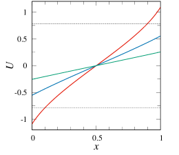
Figure 2. Shape of $U(x)$ given by (3.20). It is plotted as green, blue and red lines for $a/p=0.5,1$ and $1.5$, respectively. The dotted lines represent $U=\pm\pi/4$.

Figure 1 shows the dependence of $C$ on $a/p$, which is easily computed by the relation (3.22). In the left side of the dashed line there, condition (3.23) holds so that the synchronized solutions (3.5) are asymptotically stable in (3.2). In Fig. 2 the shape of $U(x)$ is plotted as green, blue and red lines for $a/p=0.5,1$ and $1.5$, respectively. The values of $a/(2pC)$ were numerically computed as $0.252716\ldots$, $0.525268\ldots$ and $0.886571\ldots$ for $a/p=0.5,1$ and $1.5$, respectively. In the figure we observe that $U(x)$ violates condition (3.23) for $a=1.5$ while it does not for $a/p=0.5,1$, as predicted in Fig. 1.

3.2.1. Deterministic undirected dense graph

We turn to the Kuramoto model (3.1). We begin with a deterministic undirected dense graph with

$$w_{ij}^{n}=p,\quad i,j\in[n],$$ (3.25)

which follows from (2.3) and (3.19). We carried out numerical simulations for the Kuramoto model (3.1) with $n=1000$, $\alpha_{n}=1$, $p=1$ and $a=1$. The initial values $u_{i}^{n}(0)$, $i\in[n]$, were independently randomly chosen according to the uniform distribution on $[-\pi,\pi]$. This corresponds, for instance, to a situation in which the step function

$$g(x)=u_{i}^{n}(0)\quad\mbox{for $x\in I_{i}^{n}$, $i\in[n]$,}$$

is chosen as the initial condition of the continuum limit (3.2). We took the initial condition since we want to see whether our theoretical prediction is valid for such a general one.

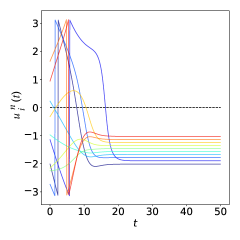
Figure 3. Numerical simulation result of the Kuramoto model (3.1) with (3.25) for $n=1000$, $\alpha_{n}=1$, $p=1$ and $a=1$: The time-history of every 100th node (from 100th to 1000th) is plotted with a different color. The nodes are lined up from bottom to top in the synchronized state.

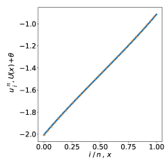
Figure 4. Comparison between $u_{i}^{n}(50)$, $i\in[n]$, in the Kuramoto model (3.1) with (3.25) and the continuum limit synchronized solution (3.27) with $a/(2pC)=0.525268\ldots$ and $\theta=-1.460872\ldots$ for $n=1000$, $\alpha_{n}=1$, $p=1$ and $a=1$. The former and latter are plotted as orange dotted and blue solid lines, respectively.

Figure 3 shows the time-history of every 100th node (from 100th to 1000th). We observe that the response rapidly converges to the synchronized state, which is given by

$$u_{i}^{n}=\arcsin\biggl{(}\frac{a(2i-1-n)}{2npC_{D}}\biggr{)}+\theta$$ (3.26)

with $n=1000$, $a/(2pC_{D})\approx a/(2pC)=0.525268\ldots$ from the above theory, where $\theta$ is estimated as

$$\theta\approx\frac{1}{n}\sum_{i=1}^{n}u_{i}^{n}(50)=-1.460872\ldots$$

from the numerical result. We also remark that the response converged to the synchronized state given by (3.26) for $a<\pi/2$ even when condition (3.24) does not hold. In Fig. 4 the response of (3.1) at $t=50$ for $a=1$ is compared with the continuum limit synchronized solution

$$u(x)=\arcsin\biggl{(}\frac{a(2x-1)}{2pC}\biggr{)}+\theta,$$ (3.27)

to which Eq. (3.26) converges with $i/n\to x$ as $n\to\infty$, with $a/(2pC)=0.525268\ldots$ and $\theta=-1.460872\ldots$. We see that both coincide almost completely, as predicted theoretically.

3.2.2. Random dense graph

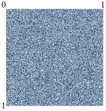
Figure 5. Pixel picture of a sampled weight matrix for the random undirected dense graph given by $w_{ij}^{n}=1$, $i,j\in[n]$, with probability (3.28) for $n=1000$ and $p=0.5$. The abscissa and ordinate represent $j/n$ and $i/n$, respectively. The color of the corresponding pixel is blue if $w_{ij}^{n}=1$ and it is white otherwise.

We next consider a random undirected dense graph given by $w_{ij}^{n}=1$ with probability

$$\mathbb{P}(j\sim i)=p,\quad i,j\in[n],$$ (3.28)

which follows from (2.4) and (3.19). Figure 5 represents the weight matrix for a numerically computed sample of the random undirected dense graph with $n=1000$ and $p=0.5$. We carried out numerical simulations for the Kuramoto model (3.1) with the weight matrix displayed in Fig. 5 for $n=1000$, $\alpha_{n}=1$ and $a=0.5$. The initial values $u_{i}^{n}(0)$, $i\in[n]$, were independently randomly chosen on $[-\pi,\pi]$.

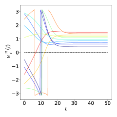
Figure 6. Numerical simulation result of the Kuramoto model (3.1) with the weight matrix displayed in Fig. 5 for $n=1000$, $\alpha_{n}=1$, $p=0.5$ and $a=0.5$. See also the caption of Fig. 3.

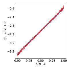
Figure 7. Comparison between $u_{i}^{n}(50)$, $i\in[n]$, in the Kuramoto model (3.1) with (3.28) and the continuum limit synchronized solution (3.27) with $a/(2pC)=0.525268\ldots$ and $\theta=1.059373\ldots$ for $a=0.5$ and $n=1000$. The former and latter are plotted as small orange disks and a blue line, respectively.

Figure 6 shows the time-history of every 100th node. We observe that the response rapidly converges to the synchronized state, which is given by (3.26) with $a/(2pC_{D})\approx a/(2pC)=0.525268\ldots$ from the above theory, where

$$\theta\approx{\color[rgb]{0,0,0}\frac{1}{n}}\sum_{i=1}^{n}u_{i}^{n}(50)=1.059373\ldots$$

from the numerical result. In Fig. 7 the response of (3.1) at $t=50$ for $a=1$ is compared with the continuum limit synchronized solution (3.27) with $a/(2pC)\color[rgb]{0,0,0}=0.525268\ldots$ and $\theta=1.059373\ldots$. We see that their agreement is good, as predicted theoretically, although small fluctuations due to randomness are found.

Figure 8. Dependence of the approximate convergence error $\Delta_{n}$ on the node number $n$ in the Kuramoto model (3.1) with (3.28) for $a=0.5$ and $T=100$.

Figure 8 shows how the convergence error of $\mathbf{u}_{n}(T)$ to $U(x)+\theta$ depends on the node number $n$ for $T=100$, where

$$\Delta_{n}^{2}= \frac{1}{n}\sum_{i=1}^{n}\left(u_{i}^{n}(100)-U\left(\frac{2i-1}{2n}\right)\right)^{2}$$

$$-\biggl{(}\frac{1}{n}\sum_{i=1}^{n}\left(u_{i}^{n}(100)-U\left(\frac{2i-1}{2n}\right)\right)\biggr{)}^{2},$$ (3.29)

which expresses an approximation for the $L^{2}(I)$ convergence error of $\mathbf{u}_{n}(T)$ as $n\to\infty$ given by

$$\min_{\theta\in\mathbb{S}^{1}}\int_{I}\left(\mathbf{u}_{n}(T)-U(x)-\theta\right)^{2}dx$$

with $T>0$ sufficiently large. Here the initial values $u_{i}^{n}(0)$, $i\in[n]$, were independently randomly chosen according to the uniform distribution on $[-\pi,\pi]$ for each $n$. We observe that the error $\Delta_{n}$ decreases as $n$ increases even though different initial conditions were taken.

3.2.3. Random sparse graph

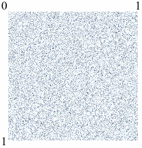
Figure 9. Pixel picture of a sampled weight matrix for the random sparse graph given by $w_{ij}^{n}=1$, $i,j\in[n]$, with probability (3.28) for $n=1000$ and $p=1$. See also the caption of Fig. 5.

We next consider a random undirected sparse graph given by $w_{ij}^{n}=1$ with probability

$$\mathbb{P}(j\sim i)=n^{-\gamma}p,\quad i,j\in[n]$$ (3.30)

which follows from (2.5) and (3.19) with $\alpha_{n}=n^{-\gamma}$, where $\gamma\in(0,0.5)$. Figure 9 represents the weight matrix for a numerically computed sample of the random undirected sparse graph with $n=1000$, $p=1$ and $\gamma=0.3$, like Fig. 5. We carried out numerical simulations for the Kuramoto model (3.1) with the weight matrix displayed in Fig. 9 for $n=1000$, $\gamma=0.3$ and $a=1$. The initial values $u_{i}^{n}(0)$, $i\in[n]$, were independently randomly chosen on $[-\pi,\pi]$.

Figure 10. Numerical simulation result of the Kuramoto model (3.1) with the weight matrix displayed in Fig. 9 for $n=1000$, $\gamma=0.3$ and $a=1$. See also the caption of Fig. 3

.

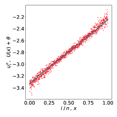
Figure 11. Comparison between $u_{i}^{n}(50)$, $i\in[n]$, in the Kuramoto model (3.1) with (3.30) and the continuum limit synchronized solution (3.27) with $a/(2pC)=0.525268\ldots$ and $\theta=1.640532\ldots$ for $a=1$ and $n=1000$: The former and latter are plotted as small orange disks and a blue line, respectively.

Figure 10 shows the time-history of every 100th node. We observe that the response rapidly converges to the synchronized state, which is given by (3.26) with $a/(2pC_{D})\approx a/(2pC)=0.525268\ldots$ from the above theory, where

$$\theta\approx\frac{1}{n}\sum_{i=1}^{n}u_{i}^{n}(50)=1.640532\ldots$$

from the numerical result, in Fig. 10. In Fig. 11 the response of (3.1) at $t=50$ for $a=1$ is compared with the continuum limit synchronized solution (3.27) with $a/(2pC)=0.525268\ldots$ and $\theta=1.640532\ldots$. We see that their agreement is good, as predicted theoretically, although some fluctuations due to randomness are found.

Figure 12. Dependence of the approximate convergence error $\Delta_{n}$ on the node number $n$ in the Kuramoto model (3.1) with (3.30) for $a=1$ and $T=100$.

Figure 12 shows the dependence of the approximate convergence error $\Delta_{n}$ given by (3.29) on the node number $n$. Here the initial values $u_{i}^{n}(0)$, $i\in[n]$, were independently randomly chosen according to the uniform distribution on $[-\pi,\pi]$ for each $n$ as in Fig. 8.. We observe that the error $\Delta_{n}$ decreases as $n$ increases even though different initial conditions were taken.

3.3. Determination of network graphs for prescribed desired solutions

We next discuss a problem for determination of a network graph such that the Kuramoto model (3.1) exhibits desired synchronized motions approximately prescribed by

$$u_{i}^{n}(t)=\Omega_{0}t+U_{0}(i/n)+\theta,\quad\theta\in\mathbb{S}^{1},\quad i\in[n],$$ (3.31)

for $n>0$ sufficiently large, where $U_{0}(x)$ is a given function and $\theta\in\mathbb{S}^{1}$ is a constant, when the natural frequency $\omega_{i}^{n}$ of the $i$th node is given by a measurable function $\omega(x)$ through (1.13) for $i\in[n]$ as in the above. The synchronized motion is precisely represented by such a formula as (3.15). We also assume the following:

• There exist two sets $I_{\pm}\subset I$ with nonzero measures such that

  $$\sin U_{0}(x)>0 x\in I_{+} \sin U_{0}(x)<0 x\in I_{-}$$ for and for ;

• $(\omega(x)-\Omega_{0})\sin U_{0}(x)\geq 0$;

• $\omega(x)-\Omega_{0}=0$ if $\sin U_{0}(x)=0$.

From the analysis of Section 3.1 we see that if condition (3.13) holds, then the family of solutions approximately given by (3.31) is asymptotically stable for $n>0$ sufficiently large.

Using (3.5), we obtain

$$\begin{split}&H_{1}(x)=\begin{cases}\displaystyle\frac{\omega(x)-\Omega_{0}}{C_{0}\sin U_{0}(x)}&\mbox{if $\sin U_{0}(x)\neq 0$;}\\ 0&\mbox{otherwise},\end{cases}\\ &H_{2}(y)=\begin{cases}H_{2+}&\mbox{if $y\in I_{+}$;}\\ H_{2-}&\mbox{if $y\in I_{-}$;}\\ 0&\mbox{if $y\notin I_{+}\cup I_{-}$}\end{cases}\end{split}$$ (3.32)

as a solution to our problem, where

$$H_{2+}=-\int_{I-}\sin U_{0}(y)dy>0,\quad H_{2-}=\int_{I+}\sin U_{0}(y)dy>0,$$

$$C_{0}=H_{2-}\int_{I_{-}}\cos U_{0}(y)dy+H_{2+}\int_{I_{+}}\cos U_{0}(y)dy.$$

Note that the relation

$$\int_{I}H_{2}(y)\sin U_{0}(y)dy=0,$$

which guarantees (3.7), holds. Thus, depending on whether the network graph $G_{n}$ is deterministic dense, random dense or random sparse, we can obtain the weight matrix $W(G_{n})$ from $W(x,y)=H_{1}(x)H_{2}(y)$ through (2.3), (2.4) or (2.5) such that the Kuramoto model (3.1) exhibits the desired motion (3.31), where for the random dense network, the function $D(u)$ and the probability $\mathbb{P}(j\to i)$ are replaced by $w_{n0}D(u)$ and

$$\mathbb{P}(j\to i)=\frac{1}{w_{n0}}\langle W(x,y)\rangle_{ij}\in[0,1],$$

respectively, if $\sup_{(x,y)\in I}H_{1}(x)H_{2}(y)>1$, where $w_{n0}>1$ is a normalized constant.

As an example, we consider the case in which the desired synchronized motion is approximately given by (3.31) with

$$\Omega_{0}=0,\quad U_{0}(x)=\begin{cases}-\frac{1}{6}\pi&\mbox{for $x\in[0,0.5]$;}\\ \frac{1}{6}\pi&\mbox{for $x\in(0.5,1]$}\end{cases}$$ (3.33)

when the natural frequencies are given by (1.13) with

$$\omega(x)=\begin{cases}\tfrac{1}{2}(x-1)&\mbox{for $x\in[0,0.5]$;}\\ \tfrac{1}{2}x&\mbox{for $x\in(0.5,1]$}.\end{cases}$$

The synchronized solution $u=U_{0}(x)+\theta$ to (3.2) with (3.33) consists of two clusters. We choose $I_{-}=[0.2,0.3]$ and $I_{+}=[0.7,0.8]$, so that

$$H_{2\pm}=0.05,\quad C_{0}=0.01\times\frac{\sqrt{3}}{2},\quad H_{1}(x)=\begin{cases}\displaystyle-C_{0}^{-1}(x-1)&\mbox{$x\in[0,0.5]$;}\\ C_{0}^{-1}x&\mbox{$x\in(0.5,1]$.}\end{cases}$$

Hence,

$$W(x,y)=\begin{cases}\displaystyle-\frac{10(x-1)}{\sqrt{3}}&\mbox{if $x\in[0,0.5]$ and $y\in[0.2,0.3]\cup[0.7,0.8]$};\\ \displaystyle\frac{10x}{\sqrt{3}}&\mbox{if $x\in(0.5,1]$ and $y\in[0.2,0.3]\cup[0.7,0.8]$};\\ 0&\mbox{otherwise.}\end{cases}$$

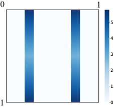
Figure 13. Pixel picture of a sampled weight matrix of the deterministic directed dense graph $G_{n}$ with $n=1000$. The shade of the corresponding pixel represents the strength of $w_{ij}^{n}$. Especially, its color is white if $w_{ij}^{n}=0$. See also the caption of Fig. 5.

Henceforth we assume that the network graph $G_{n}$ is deterministic directed dense. The other network graphs can be treated similarly, as in Sections 3.2.2 and 3.2.3. Figure 13 represents the weight matrix of $G_{n}$ with $n=1000$. Noting that

$$\frac{1}{\cos U_{i}}-2\cos U_{i}=1,\quad i\in[n],$$

we see that condition (3.18) holds as well as (3.17), so that by our general arguments to the Kuramoto model (3.1), the family of desired synchronized solutions is asymptotically stable. We carried out numerical simulations for the Kuramoto model (3.1) with the weight matrix displayed in Fig. 13 for $n=1000$, $\alpha_{n}=1$ and $a=0.5$. The initial values $u_{i}^{n}(0)$, $i\in[n]$, were independently randomly chosen on $[-\pi,\pi]$.

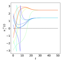
Figure 14. Numerical simulation result of the Kuramoto model (3.1) with the weight matrix displayed in Fig. 13 for $n=1000$ and $a=0.5$. See also the caption of Fig. 3.

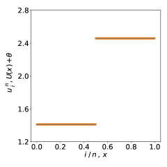
Figure 15. The snapshot of the phases $u_{i}^{n}(50)$, $i\in[n]$, in the Kuramoto model (3.1) with the weight matrix displayed in Fig. 13 for $n=1000$ and $a=0.5$. Here $\theta=1.934663\ldots$ is estimated.

Figure 14 shows the time-history of every 100th node. In Fig. 15 the snapshot of the phases $u_{i}^{n}(50)$, $i\in[n]$, is plotted. We observe that the response rapidly converges to the desired synchronized state

$$u_{i}^{n}=\begin{cases}-\frac{1}{6}\pi+\theta&\mbox{for $i\leq 500$;}\\ \frac{1}{6}\pi+\theta&\mbox{for $i>500$}\end{cases}$$

with

$$\theta\approx\frac{1}{n}\sum_{i=1}^{n}u_{i}^{n}(50)=1.934663\ldots.$$

4. Controlled Kuramoto model with natural frequencies

We next consider a modified Kuramoto model with multiple natural frequencies,

$$\frac{d}{dt}u_{i}^{n}(t)=\omega_{i}^{n}+b\sin(\bar{U}-u_{i}^{n}(t))+\frac{1}{n}\sum^{n}_{j=1}\sin\left(u_{j}^{n}(t)-u_{i}^{n}(t)\right),\quad i\in[n],$$ (4.1)

and its continuum limit

$$\frac{\partial}{\partial t}u(t,x)=\omega(x)+b\sin(\bar{U}-u(t,x))+\int_{I}\sin(u(t,y)-u(t,x))dy,\quad x\in I,$$ (4.2)

which are, respectively, special cases of (1.11) and (1.12) with $m=1$, $f(u,t)=b\sin(\bar{U}-u)$, $D(u)=\sin u$ and $W(x,y)\equiv 1$, where $\bar{U}\in\mathbb{S}^{1}$ is a constant. Similar systems were numerically studied in [38, 39]. Here the dependence of the graph on the index $k$ is dropped out, as in Section 3. A non-constant function could be taken as the desired state $\bar{U}$ (cf. Eq. (1.4)) but the analytic treatment of the continuum limit (4.2) would be very difficult.

Let $b=0$. From Section 3 we see that if there is not a constant $C$ satisfying (3.4) with $H_{\ell}(x)\equiv 1$, $\ell=1,2$, then both the continuum limit (4.2) and Kuramoto model (4.1) with $n>0$ sufficiently large do not have synchronized solutions of the forms (3.5) and (3.15), respectively. For example, when $\omega(x)=a(x-\frac{1}{2})$ as in Section 3.2, if $a>\frac{1}{2}\pi$, then such a constant $C$ does not exist. So we try to choose an adequate value of $b$ so that the modified Kuramoto model (4.1) exhibits a synchronized motion like (3.15). In this case the second term ‘$b\sin(\bar{U}-u_{i}^{n}(t))$’ is regarded as a nonlinear feedback control in (4.1) such that the coupled oscillator network (4.1) is desired to exhibit the completely synchronized state $u_{i}^{n}=\bar{U}$, $i\in[n]$.

We assume that the continuum limit (4.2) with $b\neq 0$ has a synchronized solution of the form (3.5) with $\theta=\bar{U}$. An argument similar to that of Section 3 can apply although Eq. (3.4) is replaced with

$$C-b=\int_{I}\cos U(y)dy.$$ (4.3)

So we see that if there exists a constant $C$ such that Eq. (4.3) holds, then the synchronized solution (3.5) with $\theta=\bar{U}$ exists. Moreover, the linear operator (3.9) is replaced with

$$\mathscr{L}\phi(x)=\int_{I}(\phi(y)-\phi(x))\cos(U(y)-U(x))dy-b\phi(x)\cos U(x),$$

so that

$$\langle\mathscr{L}\phi,\phi\rangle$$

$$=-\tfrac{1}{2}\int_{I^{2}}(\phi(y)-\phi(x))^{2}\cos(U(y)-U(x))dxdy-b\int\phi(x)^{2}\cos U(x)dx.$$

Hence, if condition (3.23) holds with $p=1$, then the synchronized solution (3.5) with $\theta=\bar{U}$ is asymptotically stable. Similarly, we see that if there exists a constant $C_{D}$ such that

$$C_{D}-b=\frac{1}{n}\sum_{i=1}^{n}\cos U_{i},$$

then the synchronized solution (3.15) with $\theta=\bar{U}$ exists. Since the relations (3.16) also hold, the synchronized solutions of (4.1) converges to (3.5) of (4.2) as $n\to\infty$. Moreover, we show that if condition (3.23) holds with $p=1$, then the solution (3.15) is asymptotically stable for $n>0$ sufficiently large, as in Section 3.1.

As an example, we consider the case in which $\omega(x)=a(x-\frac{1}{2})$ and $\bar{U}=\pi/6$. We have $\Omega=0$ and compute (4.3) as

$$C-b=\frac{C}{a}\left(\arcsin\left(\frac{a}{2C}\right)+\frac{a}{2C}\sqrt{1-\left(\frac{a}{2C}\right)^{2}}\right)$$

like (3.21), so that

$$a=\left(\arcsin\left(\frac{a}{2C}\right)+\frac{a}{2C}\sqrt{1-\left(\frac{a}{2C}\right)^{2}}\right)+2b\left(\frac{a}{2C}\right).$$ (4.4)

We see that if and only if

$$b\geq\frac{4a-2-\pi}{4\sqrt{2}},$$ (4.5)

then there exists a constant $C$ satisfying (4.4) and condition (3.23) with $p=1$ holds, so that the synchronized solution (3.27) with $\theta=\pi/6=0.5235987\ldots$ exists in the continuum limit (4.2) and it is asymptotically stable, along with the solution (3.26) with $\theta=\pi/6$ in the discrete model (4.1) for $n>0$ sufficiently large.

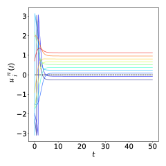
Figure 16. Numerical simulation result of the controlled Kuramoto model (4.1) with $\omega(x)=a(x-\frac{1}{2})$ for $n=1000$, $a=2$ and $b=0.506$. See also the caption of Fig. 3.

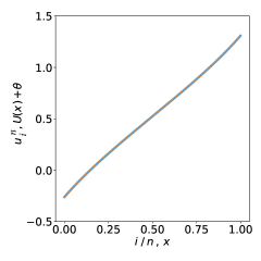
Figure 17. Comparison between $u_{i}^{n}(50)$, $i\in[n]$, to the controlled Kuramoto model (4.1) with $\omega(x)=a(x-\frac{1}{2})$ and the synchronized solution (3.27) to the continuum limit (4.2) with $a/(2C)=0.70669\ldots$ and $\theta=0$ for $n=1000$, $a=2$ and $b=0.506$. The former and latter are plotted as orange dotted and blue solid lines, respectively.

We carried out a numerical simulation for the controlled Kuramoto model (4.1) with $n=1000$, $a=2$ and

$$b=0.506>\frac{6-\pi}{4\sqrt{2}}=0.5052998\ldots,$$

which yields $a/(2C)=0.70699\ldots$ by (4.4). The initial values $u_{i}^{n}(0)$, $i\in[n]$, were independently randomly chosen on $[-\pi,\pi]$. Figure 16 shows the time-history of every 100th node. We observe that the response rapidly converges to a synchronized state. In Fig. 17 the response of (4.1) at $t=50$ for $n=1000$ is compared with the corresponding continuum limit synchronized solution (3.27). We see that both coincide almost completely, as predicted theoretically.

5. Kuramoto model with no natural frequencies on two graphs

We finally consider another modified Kuramoto model with no natural frequencies depending on two graphs,

$$\frac{d}{dt}u_{i}^{n}(t) =\frac{1}{n}\sum^{n}_{j=1}\sin\left(u_{j}^{n}(t)-u_{i}^{n}(t)\right)$$

$$\quad+\frac{K}{n\alpha_{n}}\sum^{n}_{j=1}w_{ij}\sin 2\left(u_{j}^{n}(t)-u_{i}^{n}(t)\right),\quad i\in[n],$$ (5.1)

and its continuum limit

$$\frac{\partial}{\partial t}u(t,x) =\int_{I}\sin(u(t,y)-u(t,x))dy$$

$$\quad+K\int_{I}W(x,y)\sin 2(u(t,y)-u(t,x))dy,\quad x\in I,$$ (5.2)

where $K$ is a constant. Here one of the graphs is a complete graph, and the dependence of the other graph on the index $k$ is dropped out. It is well known [42] that the Kuramoto model with no natural frequencies on a single complete graph, i.e., Eq. (5.1) with $K=0$, exhibits a complete synchronized state $u_{i}^{n}(t)=q$, $i\in[n]$, where $q\in\mathbb{S}^{1}$ is a constant. So we look for the value of $K\neq 0$ such that the complete synchronized state becomes unstable. As the second graph, we choose a $\kappa$-nearest neighbor graph given by

$$w_{ij}=\begin{cases}1&\mbox{if $|i-j|\leq\kappa n$ or $|i-j|\geq(1-\kappa)n$;}\\ 0&\mbox{otherwise}\end{cases}$$

with $0<\kappa\leq 1/2$, so that

$$W(x,y)=\begin{cases}1&\mbox{if $|x-y|\leq\kappa$ or $|x-y|\geq 1-\kappa$;}\\ 0&\mbox{otherwise.}\end{cases}$$

In particular, the graph is deterministic, undirected and dense, and $\alpha_{n}=1$ in (5.1).

We first discuss the linear stability of the complete synchronized solution $u(t,x)=q$ in (5.2), which corresponds to the solution $u_{i}^{n}(t)=q$ in (5.1). The associated linear operator $\mathscr{L}:L^{2}(I)\to L^{2}(I)$ is given by

$$\mathscr{L}\phi(x) =\int_{I}(1+2KW(x,y))\phi(y)dy-(1+4K\kappa)\phi(x).$$ (5.3)

We see that $\phi(x)=1$ is an eigenfunction of $\mathscr{L}$ associated with the zero eigenvalue. Moreover,

$$\phi(x)=\sin 2\pi\ell x,\quad\cos 2\pi\ell x$$ (5.4)

are eigenfunctions associated with the eigenvalue

$$\lambda=\frac{2K}{\pi\ell}\sin 2\pi\ell\kappa-(1+4K\kappa)$$ (5.5)

for each $\ell\in\mathbb{N}$ since

$$\int_{I}W(x,y)\sin 2\pi\ell y\,dy=\frac{1}{\pi\ell}\sin 2\pi\ell\kappa\,\sin 2\pi\ell x,$$

$$\int_{I}W(x,y)\cos 2\pi\ell ydy=\frac{1}{\pi\ell}\sin 2\pi\ell\kappa\,\cos 2\pi\ell x.$$

These eigenvalues are the only ones of $\mathscr{L}$ since the Fourier expansion of any function in $L^{2}(I)$ converges a.e. by Carleson’s theorem [4]. We compute

$$\langle\mathscr{L}\phi,\phi\rangle =\int_{I^{2}}(1+2KW(x,y))\phi(x)\phi(y)dxdy-\int_{I^{2}}(1+4K\kappa)\phi(x)^{2}dx$$

$$=-\frac{1}{2}\int_{I^{2}}(1+2KW(x,y))(\phi(x)-\phi(y))^{2}dxdy$$

$$\quad+\frac{1}{2}\int_{I^{2}}(1+2KW(x,y))(\phi(x)^{2}+\phi(y)^{2})dxdy-\int_{I^{2}}(1+4K\kappa)\phi(x)^{2}dx$$

$$=-\frac{1}{2}\int_{I^{2}}(1+2KW(x,y))(\phi(x)-\phi(y))^{2}dxdy$$

$$\quad+\int_{I^{2}}(1+2KW(x,y))\phi(x)^{2}dxdy-\int_{I^{2}}(1+4K\kappa)\phi(x)^{2}dx$$

$$=-\frac{1}{2}\int_{I^{2}}(1+2KW(x,y))(\phi(x)-\phi(y))^{2}dxdy$$

since

$$\int_{I^{2}}W(x,y)\phi(x)^{2}dx=2\kappa\int_{I}\phi(x)^{2}dx=2\kappa\int_{I^{2}}\phi(x)^{2}dxdy.$$

Hence, if $K\geq 0$, then the complete synchronized solution is linearly stable.

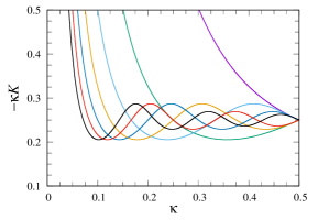
Figure 18. Boundaries of the unstable regions given by (5.6) with $\ell=1$-$7$ for the complete synchronized solutions to (5.2). The boundaries of $\ell=1,2,3,4,5,6$ and $7$ are plotted as purple, green, light blue, orange, blue, red and black lines.

Assume that $K<0$. From (5.5) we see that if

$$\frac{2K}{\pi\ell}\sin 2\pi\ell\kappa-(1+4K\kappa)>0\quad\mbox{i.e.,}\quad-\kappa K>\frac{\pi\ell\kappa}{2(2\pi\ell\kappa-\sin 2\pi\ell\kappa)}$$ (5.6)

for some $\ell\in\mathbb{N}$, then the complete synchronized solution $u(t,x)=q$ is unstable for any constant $q$. We remark that Eq. (5.6) only gives a sufficient condition for $u(t,x)=q$ to be unstable. We plot the boundaries of the unstable regions for the complete synchronized solutions given by (5.6) with $\ell=1$-$7$ in Fig. 18. By Theorem 2.7 (see also Remark 2.8(i)), the corresponding complete synchronized solutions to (5.1) for $n>0$ sufficiently large are also unstable in the region above any one of the curves in the figure.

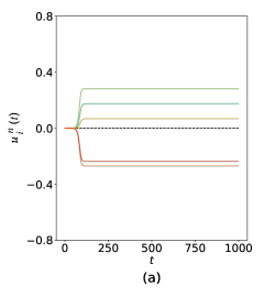
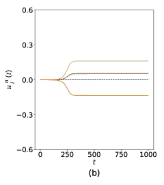
Figure 19. Numerical simulation results of the modified Kuramoto model (5.1) for $n=1000$: (a) $\kappa=1/3$ and $K=-0.7$; (b) $\kappa=1/8$ and $K=-1.7$. See also the caption of Fig. 2.

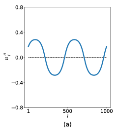
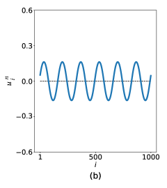
Figure 20. Steady state of the modified Kuramoto model (5.1) for $n=1000$: (a) $\kappa=1/3$ and $K=-0.7$; (b) $\kappa=1/8$ and $K=-1.7$. Here $u_{i}^{n}(1000)$, $i\in[n]$, are plotted.

We carried out numerical simulations for the modified Kuramoto model (5.1) with $n=1000$ and $\kappa=1/3$ or $1/8$. The weakest condition of (5.6) is $K<-0.621504\ldots$ with $\ell=2$ and $K<-1.64988\ldots$ with $\ell=6$ for $\kappa=1/3$ and $1/8$, respectively. The initial values $u_{i}^{n}(0)$, $i\in[n]$, were independently randomly chosen on $[-10^{-4},10^{-4}]$. So if a complete synchronized state is asymptotically stable, then the response converges to it. Figures 19(a) and (b) show the time-histories of every $100$th node for $(\kappa,K)=(1/3,-0.7)$ and $(1/8,-1.7)$, respectively. We observe that the response does not converge to a complete synchronized state for both cases, as predicted theoretically. In Figs. 20(a) and (b), $u_{i}^{n}(1000)$, $i\in[n]$, in the modified Kuramoto model (5.1) with $n=1000$, which may be regarded as the steady states, are plotted for $(\kappa,K)=(1/3,-0.7)$ and $(1/8,-1.7)$, respectively. A stable oscillatory state with two (resp. six) maxima and minima appears like the eigenfunctions (5.4) with a positive eigenvalue for the former (resp. latter) case although its existence and asymptotic stability is not obtained theoretically unlike the previous two examples.

Appendix A Proof of Theorem 2.1

In this appendix, we extend arguments in the proof of Theorem 3.1 of [18] and prove Theorem 2.1. Let $L_{f}$ and $L_{k}$ be, respectively, the Lipschitz constants of $f(\cdot,t)$ and $D_{k}(\cdot)$ for $k\in[m]$, and let

$$L_{D}=\max_{k\in[m]}L_{k}.$$

Let $\|\cdot\|$ stand for the norm in $L^{2}(I)$.

Proof of Theorem 2.1.

Let

$$T=\left(2(L_{f}+mL_{D}(C_{2}+\|W\|_{L^{2}(I^{2})}))\right)^{-1}.$$ (A.1)

Let $\mathscr{F}=C(0,T;L^{2}(I))$ and define

$$K(\mathbf{u})(t)=g+\sum_{k=1}^{m}\int_{0}^{t}\biggl{(}f(u(s,\cdot),s)+\int_{I}W(\cdot,y)D_{k}(u(s,y)-u(s,\cdot))dy\biggr{)}ds$$

for $\mathbf{u}\in\mathscr{F}$. Obviously, if $\mathbf{u}\in\mathscr{F}$, then $K(\mathbf{u})\in\mathscr{F}$. We easily see that a fixed point of the map $K:\mathscr{F}\to\mathscr{F}$, i.e.,

$$\mathbf{u}=K(\mathbf{u}),$$

gives a solution to the IVP of (1.8) with (1.9). In the following we show that $K$ is a contraction on $\mathscr{F}$, so that by the contraction map theorem (see, e.g., Theorem 2.2 in Chapter 2 of [10]) it has a unique fixed point in $\mathscr{F}$ and the IVP of (1.8) with (1.9) has a unique solution.

For any $\mathbf{u}(t),\mathbf{v}(t)\in\mathscr{F}$, by the Lipschitz continuity of $f$ and $D_{k}$, we compute

$$\|K(\mathbf{u})-K(\mathbf{v})\|=\max_{t\in[0,T]}\|K(\mathbf{u}(t))-K(\mathbf{v}(t))\|$$

$$\leq\max_{t\in[0,T]}\int_{0}^{t}\biggl{\|}f(u(s,\cdot),s)-f(v(s,\cdot),s)$$

$$\quad+\sum_{k=1}^{m}\int_{I}W(\cdot,y)(D_{k}(u(s,y)-u(s,\cdot))-D_{k}(v(s,y)-v(s,\cdot))dy\biggr{\|}ds$$

$$\leq T\max_{t\in[0,T]}\biggl{\|}L_{f}|u(t,\cdot)-v(t,\cdot)|$$

$$\quad+L_{D}\sum_{k=1}^{m}\int_{I}W(\cdot,y)|u(t,y)-u(t,\cdot)-v(t,y)+v(t,\cdot)|dy\biggr{\|}$$

$$\leq T\max_{t\in[0,T]}\biggl{(}L_{f}\|\mathbf{u}(t)-\mathbf{v}(t)\|+L_{D}\sum_{k=1}^{m}\biggl{(}\biggl{\|}\int_{I}W(\cdot,y)|u(t,\cdot)-v(t,\cdot)|dy\biggr{\|}$$

$$\quad+\biggl{\|}\int_{I}W(\cdot,y)|u(t,y)-v(t,y)|dy\biggr{\|}\biggr{)}.$$

Noting that by (2.2)

$$\biggl{\|}\int_{I}W(\cdot,y)|u(t,\cdot)-v(t,\cdot)|dy\biggr{\|}\leq C_{2}\|\mathbf{u}(t)-\mathbf{v}(t)\|$$

and by Schwarz’ inequality

$$\biggl{\|}\int_{I}W(\cdot,y)|u(t,y)-v(t,y)|dy\biggr{\|}\leq\|W\|_{L^{2}(I^{2})}\,\|\mathbf{u}(t)-\mathbf{v}(t)\|,$$

we obtain

$$\|K(\mathbf{u})-K(\mathbf{v})\|$$

$$\leq T(L_{f}+mL_{D}(C_{2}+\|W\|_{L^{2}(I^{2})}))\|\mathbf{u}(t)-\mathbf{v}(t)\|=\frac{1}{2}\|\mathbf{u}(t)-\mathbf{v}(t)\|.$$

Here the last equality in the above equation holds due to (A.1). Thus, the IVP of (1.8) with (1.9) has a unique solution $\bar{\mathbf{u}}(t)$ on $[0,T]$. Using the standard arguments given in the last paragraph in the proof of Theorem 3.1 of [18], we can extend the solution $\bar{\mathbf{u}}(t)$ to $(-\infty,\infty)$ and show that it is continuously differentiable. Actually, for example, the right-hand-side of (1.8) is continuous if $\bar{\mathbf{u}}\in C(\mathbb{R};L^{2}(I))$. Moreover, since $K:\mathscr{F}\to\mathscr{F}$ is a uniform contraction and depends on $g$ continuously, the unique solution is a continuous function of $g$. Thus, we complete the proof. ∎

Appendix B Proof of Theorem 2.3

In this appendix, we extend arguments in the proof of Theorem 3.1 of [27] and prove Theorem 2.3. Henceforth we assume that the hypotheses of Theorem 2.3 hold. So there exists a positive constant $C_{D}$ such that

$$D_{k}(u)<C_{D}\quad\mbox{for $u\in\mathbb{R}$ and $k\in[m]$.}$$

Changing the order of the graphs if necessary, we assume that for some $m_{\mathrm{d}}\in\{0\}\cup[m]$, $G_{kn}$ is a deterministic or random graph for $n\in\mathbb{N}$ depending on whether $k\leq m_{\mathrm{d}}$ or $k>m_{\mathrm{d}}$. All of $G_{kn}$, $k\in[m]$, are random if $m_{\mathrm{d}}=0$, and deterministic if $m_{\mathrm{d}}=m$. We average the coefficients appearing in the second term in the right-hand-side of (1.6) for $k\in[m]\setminus[m_{\mathrm{d}}]$ as

$$\frac{1}{n\alpha_{kn}}\mathbb{E}[w_{ij}^{kn}]=\frac{1}{n}\bar{W}_{ij}^{kn},\quad\bar{W}_{ij}^{kn}=\langle\tilde{W}\rangle_{ij}^{n},$$

where $\alpha_{kn}=1$ and $\tilde{W}=W$ when $G_{kn}$ is dense, and consider the averaged model

$$\frac{d}{dt}v_{i}^{n}(t) =f(v_{i}^{n},t)+\sum^{m_{\mathrm{d}}}_{k=1}\frac{1}{n}\sum^{n}_{j=1}w_{ij}^{kn}D_{k}(v_{j}^{n}(t)-v_{i}^{n}(t))$$

$$\quad+\sum^{m}_{k=m_{\mathrm{d}}+1}\frac{1}{n}\sum^{n}_{j=1}\bar{W}_{ij}^{kn}D_{k}(v_{j}^{n}(t)-v_{i}^{n}(t)),\quad i\in[n].$$ (B.1)

Let $u_{n}(t)$ and $v_{n}(t)$ denote the solutions to the IVPs of (1.6) and (B.1) with (1.10) and

$$v_{i}^{n}(0)=u_{i0}^{n},$$ (B.2)

respectively. We adopt the discrete $L^{2}$-norm

$$\|u_{n}\|_{2,n}:=\biggl{(}\frac{1}{n}\sum_{i=1}^{n}(u_{i}^{n})^{2}\biggr{)}^{1/2}.$$

We obtain the following estimate on the difference between the solutions $u_{n}(t)$ and $v_{n}(t)$.

Lemma B.1.

Suppose that $\gamma_{\mathrm{max}}:=\max_{k\in[m]}\gamma_{k}\in(0,\frac{1}{2})$. Then for any $T>0$ and $\delta\in(0,\tfrac{1}{2}-\gamma_{\rm max})$ we have

$$\lim_{n\rightarrow\infty}n^{\frac{1}{2}-\gamma_{\rm max}-\delta}\max_{t\in[0,T]}\|u_{n}(t)-v_{n}(t)\|_{2,n}=0\quad\mbox{a.s.}$$ (B.3)

In particular,

$$\lim_{n\rightarrow\infty}\max_{t\in[0,T]}\|u_{n}(t)-v_{n}(t)\|_{2,n}=0\quad\mbox{a.s.}$$

Proof.

Let $\psi_{i}^{n}:=v_{i}^{n}-u_{i}^{n}$. Subtracting (1.6) from (B.1), multiplying the resulting equation by $n^{-1}\psi_{i}^{n}$, and summing over $i\in[n]$, we obtain

$$\frac{1}{2}\frac{d}{dt}\|\psi_{n}\|^{2}_{2,n}=I_{1}+I_{2}+I_{3},$$ (B.4)

where

$$I_{1}= \frac{1}{n}\sum^{n}_{i=1}(f(v_{i}^{n},t)-f(u_{i}^{n},t))\psi_{i}^{n},$$

$$I_{2}= \sum^{m}_{k=m_{\mathrm{d}}+1}\frac{1}{n^{2}\alpha_{kn}}\sum^{n}_{i,j=1}(\alpha_{kn}\bar{W}_{ij}^{kn}-w_{ij}^{kn})D_{k}(v_{j}^{n}-v_{i}^{n})\psi_{i}^{n},$$

$$I_{3}= \sum^{m}_{k=1}\frac{1}{n^{2}\alpha_{kn}}\sum^{n}_{i,j=1}w_{ij}^{kn}[D_{k}(v_{j}^{n}-v_{i}^{n})-D_{k}(u_{j}^{n}-u_{i}^{n})]\psi_{i}^{n}.$$

The Lipschitz continuity of $f$ in $u$ immediately yields

$$|I_{1}|\leq L_{f}\|\psi_{n}\|^{2}_{2,n}.$$ (B.5)

Using the Lipschitz continuity of $D_{k}$ and the triangle inequality, we have

$$|I_{3}| \leq\sum^{m}_{k=1}\frac{1}{n^{2}\alpha_{kn}}\sum^{n}_{i,j=1}w_{ij}^{kn}L_{D}(|\psi_{n,i}|+|\psi_{n,j}|)|\psi_{n,i}|$$

$$\leq\sum^{m}_{k=1}\frac{L_{D}}{n^{2}\alpha_{kn}}\biggl{(}\frac{3}{2}\sum^{n}_{i,j=1}w_{ij}^{kn}\psi_{n,j}^{2}+\frac{1}{2}\sum^{n}_{i,j=1}w_{ij}^{kn}\psi_{n,j}^{2}\biggr{)}$$ (B.6)

since $|\psi_{i}^{n}|\,|\psi_{j}^{n}|\leq(|\psi_{i}^{n}|^{2}+|\psi_{j}^{n}|^{2})/2$. From (2.6) we have

$$\begin{split}&\frac{1}{n^{2}\alpha_{kn}}\sum^{n}_{i,j=1}w_{ij}^{kn}\,\psi^{2}_{n,i}\leq C_{1}\|\psi\|^{2}_{n,2},\\ &\frac{1}{n^{2}\alpha_{kn}}\sum^{n}_{i,j=1}w_{ij}^{kn}\,\psi^{2}_{n,j}\leq C_{2}\|\psi\|^{2}_{n,2}\end{split}$$ (B.7)

for $k\in[m_{\mathrm{d}}]$ since $\alpha_{kn}=1$. Proceeding as in the proof of Theorem 4.1 of [27] and using (2.7), we obtain

$$\begin{split}&\frac{1}{n^{2}\alpha_{kn}}\sum^{n}_{i,j=1}w_{ij}^{kn}\psi^{2}_{n,i}\leq(1+C_{1})\|\psi\|^{2}_{n,2}\quad\text{a.s.},\\ &\frac{1}{n^{2}\alpha_{kn}}\sum^{n}_{i,j=1}w_{ij}^{kn}\psi^{2}_{n,j}\leq(1+C_{2})\|\psi\|^{2}_{n,2}\quad\text{a.s.}\end{split}$$ (B.8)

for $k\in[m]\setminus[m_{\mathrm{d}}]$ and $n\gg 1$. Substituting (B.7) and (B.8) into (B.6) yields

$$|I_{3}|\leq L_{D}\biggl{(}2(m-m_{\mathrm{d}})+\frac{3m}{2}C_{1}+\frac{m}{2}C_{2}\biggr{)}\|\psi\|^{2}_{n,2}\quad\text{a.s.}$$ (B.9)

It remains to estimate $|I_{2}|$. Define the random variables

$$Z_{kn,i}(t)=\frac{1}{n}\sum^{n}_{j=1}b_{ij}^{kn}(t)\eta_{ij}^{kn},\quad i\in[n],$$

for $k\in[m]\setminus[m_{\mathrm{d}}]$, where

$$b_{ij}^{kn}(t)=D_{k}(v_{j}^{n}(t)-v_{i}^{n}(t)),\quad\eta_{ij}^{kn}=w_{ij}^{kn}-\alpha_{kn}\bar{W}_{ij}^{kn}.$$

Noting that

$$\frac{Z_{kn,i}(t)}{\alpha_{kn}}\psi_{i}^{n}(t)\leq\frac{1}{2}\biggl{(}\biggl{(}\frac{Z_{kn,i}(t)}{\alpha_{kn}}\biggr{)}^{2}+\psi_{i}^{n}(t)^{2}\biggr{)},$$

we have

$$|I_{2}|= \biggl{|}\sum^{m}_{k=m_{\mathrm{d}}+1}\frac{1}{n\alpha_{kn}}\sum^{n}_{i=1}Z_{kni}(t)\psi_{i}^{n}(t)\biggr{|}$$

$$\leq \sum^{m}_{k=m_{\mathrm{d}}+1}\frac{1}{2\alpha^{2}_{kn}}\|Z_{kn}(t)\|^{2}_{2,n}+\frac{m-m_{\mathrm{d}}}{2}\|\psi_{n}(t)\|^{2}_{2,n},$$ (B.10)

where $Z_{kn}=(Z_{kn,1},Z_{kn,2},\ldots,Z_{kn,n})$. Thus, it follows from (B.4), (B.5), (B.9) and (B.10) that

$$\frac{d}{dt}\|\psi_{n}(t)\|^{2}_{2,n}\leq L\|\psi_{n}(t)\|^{2}_{2,n}+\sum^{m}_{k=m_{\mathrm{d}}+1}\frac{1}{\alpha_{kn}^{2}}\|Z_{kn}(t)\|^{2}_{2,n},$$ (B.11)

where

$$L=2L_{f}+mL_{D}(3C_{1}+C_{2})+(m-m_{\mathrm{d}})(4L_{D}+1).$$

Using Gronwall’s inequality for (B.11), we obtain

$$\max_{t\in[0,T]}\|\psi_{n}(t)\|_{2,n}^{2}\leq\sum^{m}_{k=m_{\mathrm{d}}+1}\frac{2L}{\alpha^{2}_{kn}}e^{LT}\int^{T}_{0}e^{-Ls}\|Z_{kn}(s)\|^{2}_{2,n}ds.$$ (B.12)

We proceed as in the proof of Theorem 4.1 of [27] again and estimate

$$\int^{T}_{0}e^{-Ls}\|Z_{kn}(s)\|^{2}_{2,n}ds\leq\frac{C_{3}}{n}\quad\text{a.s.}$$ (B.13)

for some $C_{3}>0$, after some lengthy arguments. Combining (B.12) and (B.13) and noting that $\alpha_{kn}=n^{-\gamma_{k}}$, we have

$$\max_{t\in[0,T]}\|\psi_{n}(t)\|^{2}_{2,n}\leq \frac{2LC_{3}}{n}e^{LT}\sum^{m}_{k=m_{\mathrm{d}}+1}\alpha_{kn}^{-2}$$

$$\leq 2C_{3}e^{LT}(m-m_{\mathrm{d}})n^{-(1-2\gamma_{\mathrm{max}})}\quad\text{a.s.},$$ (B.14)

which yields (B.3). ∎

We rewrite the averaged model (B.1) and the initial condition (B.2) as

$$\frac{\partial}{\partial t}v_{n}(t,x)= f(v_{n}(t,x),t)+\sum_{k=1}^{m_{\mathrm{d}}}\int_{I}W_{kn}(x,y)D_{k}(v_{n}(t,y)-v_{n}(t,x))dy$$

$$+\sum_{k=m_{\mathrm{d}}+1}^{m}\int_{I}\bar{W}_{kn}(x,y)D_{k}(v_{n}(t,y)-v_{n}(t,x))dy$$ (B.15)

and

$$v_{n}(0,x)=g_{n}(x):=\sum_{i=1}^{n}g_{i}^{n}\mathbf{1}_{I_{i}^{n}}(x),$$ (B.16)

where

$$W_{kn}(x,y)=\sum_{i=1}^{n}\langle W_{k}\rangle_{ij}^{n}\mathbf{1}_{I_{i}^{n}\times I_{j}^{n}}(x,y),$$

$$\bar{W}_{kn}(x,y)=\sum_{i=1}^{n}\langle\tilde{W}_{k}\rangle_{ij}^{n}\mathbf{1}_{I_{i}^{n}\times I_{j}^{n}}(x,y).$$

Proof of Theorem 2.3.

Thanks to Lemma B.1, we only have to prove that the solution $v_{n}(t,x)$ to the IVP of the averaged model (B.15) with (B.16) converges to the solution $u(t,x)$ of the IVP of the continuum limit (1.8) with (1.9). We follow the proof of Theorem 5.1 of [27] with some modifications.

Let $\psi_{n}(t,x)=u(t,x)-v_{n}(t,x)$. Subtracting (B.15) from (1.8), multiplying the resulting equation by $\psi_{n}(t,x)$ and integrating it over $I$, we have

$$\frac{1}{2}\frac{d}{dt}\|\psi_{n}(t,\cdot)\|^{2}$$

$$=\int_{I}(f(u(t,x),t)-f(v_{n}(t,x))\psi_{n}(t,x)dx$$

$$\quad+\sum_{k=1}^{m}\int_{I^{2}}W_{k}(x,y)[D_{k}(u(t,y)-u(t,x))-D_{k}(v_{n}(t,y)-v_{n}(t,x))]\psi_{n}(t,x)dxdy$$

$$\quad+\sum_{k=1}^{m_{\mathrm{d}}}\int_{I^{2}}(W_{k}(x,y)-W_{kn}(x,y))D_{k}(v_{n}(t,y)-v_{n}(t,x))]\psi_{n}(t,x)dxdy$$

$$\quad+\sum_{k=m_{\mathrm{d}}+1}^{m}\int_{I^{2}}(W_{k}(x,y)-\bar{W}_{kn}(x,y))D_{k}(v_{n}(t,y)-v_{n}(t,x))]\psi_{n}(t,x)dxdy.$$ (B.17)

By the Lipschitz continuity of $f$

$$\biggl{|}\int_{I}(f(u(t,x),t)-f(v_{n}(t,x))\psi_{n}(t,x)dx\biggr{|}\leq L_{f}\|\psi_{n}(t,\cdot)\|^{2}.$$ (B.18)

Using Young’s inequality and Fubini’s theorem along with the Lipschitz continuity of $D_{k}$, (2.1) and (2.2), we have

$$\biggl{|}\int_{I^{2}}W_{k}(x,y)[D(u(t,y)-u(t,x))-D(v_{n}(t,y)-v_{n}(t,x))]\psi_{n}(t,x)dxdy\biggr{|}$$

$$\leq L_{D}\biggl{|}\int_{I^{2}}W_{k}(x,y)(|\psi_{n}(t,y)|+|\psi_{n}(t,x)|)|\psi_{n}(t,x)|dxdy\biggl{|}$$

$$\leq\frac{1}{2}L_{D}(3C_{1}+C_{2})\|\psi_{n}(t,\cdot)\|^{2}$$ (B.19)

for $k\in[m]$. Using Young’s inequality and the boundedness of $D_{k}$, we have

$$\biggl{|}\int_{I^{2}}(W_{k}(x,y)-W_{kn}(x,y))D(v_{n}(t,y)-v_{n}(t,x))\psi_{n}(t,x)dxdy\biggl{|}$$

$$\leq\frac{C_{D}}{2}(\|W_{n}-W_{kn}\|_{L^{2}(I^{2})}^{2}+\|\psi_{n}(t,\cdot)\|^{2})$$ (B.20)

for $k\in[m_{\mathrm{d}}]$ and

$$\biggl{|}\int_{I^{2}}(W_{k}(x,y)-\bar{W}_{kn}(x,y))D(v_{n}(t,y)-v_{n}(t,x))\psi_{n}(t,x)dxdy\biggl{|}$$

$$\leq\frac{C_{D}}{2}(\|W_{n}-\bar{W}_{kn}\|_{L^{2}(I^{2})}^{2}+\|\psi_{n}(t,\cdot)\|^{2})$$ (B.21)

for $k\in[m]\setminus[m_{\mathrm{d}}]$.

Combining (B.17)-(B.21), we have

$$\frac{d}{dt}\|\psi_{n}(t,\cdot)\|^{2}\leq L_{2}\|\psi_{n}(t,\cdot)\|^{2}+C_{D}\sum_{k=1}^{m_{\mathrm{d}}}\|W_{n}-W_{kn}\|_{L^{2}(I^{2})}^{2}$$

$$+C_{D}\sum_{k=m_{\mathrm{d}}+1}^{m}\|W_{n}-\bar{W}_{kn}\|_{L^{2}(I^{2})}^{2},$$

where $L_{2}=2L_{f}+m(L_{D}(3C_{1}+C_{2})+C_{D})$. Applying Gronwall’s inequality to the above equation, we obtain

$$\sup_{t\in[0,T]}\|\psi_{n}(t,\cdot)\|^{2}\leq e^{L_{2}T}\biggl{(}\|g-g_{n}\|+C_{D}\sum_{k=1}^{m_{\mathrm{d}}}\|W_{n}-W_{kn}\|_{L^{2}(I^{2})}^{2}$$

$$+C_{D}\sum_{k=m_{\mathrm{d}}+1}^{m}\|W_{n}-\bar{W}_{kn}\|_{L^{2}(I^{2})}^{2}\biggr{)}.$$

Obviously, $\|W_{n}-W_{kn}\|_{L^{2}(I^{2})}\to 0$ as $n\to\infty$ for $k\in[m_{\mathrm{d}}]$. We also show that $\|W_{n}-\bar{W}_{kn}\|_{L^{2}(I^{2})}\to 0$ as $n\to 0$ for $k\in[m]\setminus[m_{\mathrm{d}}]$, as in the proof of Theorem 5.1 of [27]. This completes the proof. ∎

References

- [1] A. Allen-Perkins, T.A. de Assis,J.M. Pastor and R.F.S. Andrade, Relaxation time of the global order parameter on multiplex networks: The role of interlayer coupling in Kuramoto oscillators, Phys. Rev. E, 96 (2017), 042312.
- [2] D.M. Abrams and S.H. Strogatz, Chimera states in a ring of nonlocally coupled oscillators, Internat. J. Bifur. Chaos, 16 (2006), 21–37.
- [3] E. Brown, J. Moehils and P. Holmes, On the phase reduction and response dynamics of neural oscillator populations, Neural Comput., 16 (2004), 673–715.
- [4] L. Carleson, On convergence and growth of partial sums of Fourier series, Acta Mathematica, 116 (1966), 135–157.
- [5] H. Chiba, A proof of the Kuramoto conjecture for a bifurcation structure of the infinite-dimensional Kuramoto model, Ergodic Theory Dynam. Systems, 35 (2015), 762–834.
- [6] H. Chiba and G.S. Medvedev, The mean field analysis of the Kuramoto model on graphs I: The mean field equation and transition point formulas, Discrete Contin. Dyn. Syst., 39 (2019), 131–155.
- [7] H. Chiba and G.S. Medvedev, The mean field analysis of the Kuramoto model on graphs II: Asymptotic stability of the incoherent state, center manifold reduction, and bifurcations, Discrete Contin. Dyn. Syst., 39 (2019), 3897–3921.
- [8] H. Chiba, G.S. Medvedev and M.S. Mizuhara, Bifurcations in the Kuramoto model on graphs, Chaos, 28 (2018), 073109.
- [9] H. Chiba and I. Nishikawa, Center manifold reduction for large populations of globally coupled phase oscillators, Chaos, 28 (2011), 043103.
- [10] S.-N. Chow and J.K. Hale, Methods of Bifurcation Theory, Springer, New York, 1982.
- [11] E.A. Coddington and N. Levinson, Theory of Ordinary Differential Equations, McGraw-Hill, New York, 1955.
- [12] F. Dorfler and F. Bullo, Synchronization and transient stability in power networks and non-uniform Kuramoto oscillators, SIAM J. Control Optim., 50 (2012), 1616–1642.
- [13] S. Gao and P.E. Caines, Graphon control of large-scale networks of linear systems, IEEE Trans. Automat. Contr., 65 (2020), 4090–4105.
- [14] S. Gao and P.E. Caines, Subspace decomposition for graphon LQR: Applications to VLSNs of harmonic oscillators, IEEE Trans. Control. Netw. Syst., 8 (2021), 576–586.
- [15] S. Gao and B. Wu, On input-to-state stability for stochastic coupled control systems on networks, Appl. Math. Comp., 262 (2015), 90–101.
- [16] T. Girnyk, M. Hasler and Y. Maistrenko, Multistability of twisted states in non-locally coupled Kuramoto-type models, Chaos, 22 (2012), 013114.
- [17] G.H. Golub and C.F. Van Loan, Matrix Computations, 4th ed., The Johns Hopkins University Press, Baltimore, MD, 2013.
- [18] D. Kaliuzhnyi-Verbovetskyi and G. S. Medvedev, The semilinear heat equation on sparse random graphs, SIAM J. Math. Anal., 49 (2017), no. 2, 1333-1355.
- [19] R. Kumar and A. Singh, Consensus dynamics on weighted multiplex networks: a long-range interaction perspective, J. Stat. Mech. Theory Exp. 2019 (2019), 113402.
- [20] Y. Kuramoto, Chemical Oscillations, Waves, and Turbulence, Springer, Berlin, 1984.
- [21] Y. Kuramoto and D. Battogtokh, Coexistence of coherence and incoherence in nonlocally coupled phase oscillators, Nonlinear Phenom. Complex Syst., 5 (2002), 380–385.
- [22] C.R. Laing and C.C. Chow, Stationary bumps in networks of spiking neurons, Neural Comput., 13 (2001), 1473–1494.
- [23] L. Lovász, Large Networks and Graph Limits, AMS, Providence RI, 2012.
- [24] G.S. Medvedev, Stochastic stability of continuous time consensus protocols, SIAM J. Control Optim., 50 (2012), 1859–1885.
- [25] G.S. Medvedev, The nonlinear heat equation on dense graphs and graph limits, SIAM J. Math. Anal., 46 (2014), 2743–2766.
- [26] G.S. Medvedev, The nonlinear heat equation on W-random graphs, Arch. Ration. Mech. Anal., 212 (2014), 781–803.
- [27] G.S. Medvedev, The continuum limit of the Kuramoto model on sparse random graphs, Comm. Math. Sci., 17 (2019), 883–898.
- [28] G.S. Medvedev and S. Zhuravytska, The geometry of spontaneous spiking in neuronal networks, J. Nonlinear Sci., 22 (2012), 689–725.
- [29] A. Millán, J.K. Torres and G. Bianconi, Explosive higher-order Kuramoto dynamics on simplicial complexes, Phys. Rev. Lett., 124 (2020), 218301.
- [30] I. Omelchenko, B. Riemenschneider, P. Hövel, Y. Maistrenko and E. Schöll, Transition from spatial coherence to incoherence in coupled chaotic systems, Phys. Rev. E, 85 (2012), 026212.
- [31] O.E. Omel’chenko, M. Wolfrum, S. Yanchuk, Y. Maistrenko and O. Sudakov, Stationary patterns of coherence and incoherence in two-dimensional arrays of non-locally-coupled phase oscillators, Phys. Rev. E, 85 (2012), 036210.
- [32] E. Ott and T.M. Antonsen, Low dimensional behavior of large systems of globally coupled oscillators, Chaos, 18 (2008), 037113.
- [33] J.R. Phillips, H.S.J. van der Zant, J. White and T.P. Orlando, Influence of induced magnetic fields on the static properties of Josephson-junction arrays, Phys. Rev. B, 47 (1993), 5219–5229.
- [34] Q.S. Ren, Q.F. Long and J. Zhao, Symmetry and symmetry breaking in a Kuramoto model induced on a Möbius strip, Phys. Rev. E, 87 (2013), 022811.
- [35] D.C. Roberts, Linear reformulation of the Kuramoto model of self-synchronizing coupled oscillators, Phys. Rev. E, 77 (2008), 031114.
- [36] M. Sadilek and S. Thurner, Physiologically motivated multiplex Kuramoto model describes phase diagram of cortical activity, Sci. Rep., 5 (2015), 10015.
- [37] S. Shima and Y. Kuramoto, Rotating spiral waves with phase-randomized core in nonlocally coupled oscillators, Phys. Rev. E, 69 (2004), 036213.
- [38] P. S. Skardal and A. Arenas, Control of coupled oscillator networks with application to microgrid technologies, Science Advances, 1 (2015), e1500339.
- [39] P. S. Skardal and A. Arenas, On controlling networks of limit-cycle oscillators, Chaos, 26 (2016), 094812.
- [40] D. Tanaka and Y. Kuramoto, Complex Ginzburg-Landau equation with nonlocal coupling, Phys. Rev. E, 68 (2003), 026219.
- [41] D.J. Watts and S.H. Strogatz, Collective dynamics of small-world networks, Nature, 393 (1998), 440–442.
- [42] D.A. Wiley, S.H. Strogatz and M. Girvan, The size of the sync basin, Chaos, 16 (2006), 015103.