Uniformly Perfect Sets, Hausdorff Dimension, and Conformal Capacity

Abstract.

Using the definition of uniformly perfect sets in terms of convergent sequences, we apply lower bounds for the Hausdorff content of a uniformly perfect subset $E$ of $\mathbb{R}^{n}$ to prove new explicit lower bounds for the Hausdorff dimension of $E.$ These results also yield lower bounds for capacity test functions, which we introduce, and enable us to characterize domains of ${\mathbb{R}}^{n}\,$ with uniformly perfect boundaries. Moreover, we show that an alternative method to define capacity test functions can be based on the Whitney decomposition of the domain considered.

In memoriam: Pentti Järvi 1942- 2021

1. Introduction

Conformal invariants, in particular the modulus of a curve family and the conformal capacity of a condenser, are fundamental tools of geometric function theory and quasiconformal mappings [9, 10, 11, 12, 31]. For applications, many upper and lower bounds for conformal invariants have been derived in terms of various geometric functionals. All this research shows that the metric structure of the boundary has a strong influence on the intrinsic geometry of the domain of the mappings studied. Indeed, many results originally proven for functions defined in the unit ball $\mathbb{B}^{n}$ of ${\mathbb{R}}^{n},n\geq 2,$ can be extended to the case of subdomains $G\subset{\mathbb{R}}^{n}$ if the boundary $\partial G$ is ”thick enough” in the sense of capacity, or, more precisely, if the boundary is uniformly perfect. The thickness of the boundary has a strong influence on the intrinsic geometry of the domain and thus it also gives a restriction on the oscillation of a function defined in $G.$ We give several new characterizations of uniformly perfect sets.

A condenser is a pair $(G,E)$ where $G\subset{\mathbb{R}}^{n}$, $n\geq 2$, is a domain and $E\subset G$ is a compact set [9, 11, 12]. A compact set $E\subset{\mathbb{R}}^{n}$ is of conformal capacity zero if, for some closed ball $B\subset{\mathbb{R}}^{n}\setminus E\,,$ the condenser $({\mathbb{R}}^{n}\setminus B,E)$ has capacity zero, written as $\mathrm{cap}\,(E)=0$ with notations of Definition 4.1. Sets of capacity zero are very thin, their Hausdorff dimension is zero [26, p.120, Cor. 2], [12, Lemma 9.11], and they often have the role of negligible exceptional sets in potential theory or geometric function theory. Note that, due to the Möbius invariance of the conformal capacity, the notions of zero and positive capacity immediately extend to compact subsets of the Möbius space $\overline{{\mathbb{R}}}^{n}={\mathbb{R}}^{n}\cup\{\infty\}$.

Here our goal is to study those subsets of ${\mathbb{R}}^{n}$ that have a positive capacity instead. However, the structure of sets of positive capacity can sometimes be highly dichotomic, for instance, in the case of $E_{1}\cup E_{2}$ where $E_{1}\subset{\mathbb{R}}^{2}$ is a segment and $E_{2}$ is a point not contained in $E_{1}$. This kind of a dichotomy makes working with these sets difficult, but a subclass of sets with positive capacity, uniformly perfect sets, has certain natural properties useful for our purposes. During the past two decades, uniformly perfect sets have become ubiquitous for instance in geometric function theory [3, 10], analysis on metric spaces [13, 18], hyperbolic geometry [4, 16] and in the study of complex dynamics and Kleinian groups [7, 27].

We begin by giving a variant of the definition of uniformly perfect sets in terms of convergent sequences as follows. For $0<c<1,$ let ${\rm UP}_{n}(c)$ denote the collection of compact sets $E$ in $\mathbb{R}^{n}$ with ${\operatorname{card}\,}(E)\geq 2$ satisfying the condition

$$\{x\in E:cr<|x-a|<r\}\neq\emptyset\quad\text{for all}~{}a\in E\quad\text{and}\quad 0<r<d(E)/2\,.$$

We say that a set is uniformly perfect if it is in the class ${\rm UP}_{n}(c)$ for some $c\in(0,1).$

Theorem 1.1.

(T. Sugawa [29, Proposition 7.4]) Let $E\in{\rm UP}_{n}(c)$ for some $0<c<1.$ Then for every $a\in E,~{}a\neq\infty,$ the Hausdorff content of $E$ has the following lower bound

$$\Lambda^{\beta}(E\cap{\overline{B}^{n}}(a,r))\geq\frac{r^{\beta}}{2\cdot 3^{n}},\quad 0<r<d(E)/2,~{}\text{where}~{}\beta=\frac{\log 2}{\log(3/c)}.$$

Moreover, the Hausdorff dimension $\dim_{H}(E)$ of $E$ is at least $(\log 2)/\log(3/c).$

The explicit bounds we obtain in this paper depend on the above result of Sugawa, given here with a modified form of the constant $\beta.$ Moreover, we also apply ideas from the work of Reshetnyak [25, 26] and Martio [19], see also Remark 5.4, but now the constants are explicit which is crucial for what follows. In the study of uniformly perfect sets, similar methods were also applied by Järvi and Vuorinen [14, Thm 4.1, p. 522]. Our results here yield explicit constants for several characterizations of uniform perfectness such as the following main result.

Theorem 1.2.

Let $E\in{\rm UP}_{n}(c)$ for some $0<c<1.$ Then for every $a\in E,~{}a\neq\infty,$ and all $r\in(0,d(E))$ the following lower bound for the conformal capacity ${\rm cap}(a,E,r)$ of the condenser $(B^{n}(a,2r),E\cap\overline{B}^{n}(a,r))$ holds

$${\rm cap}(a,E,r)\geq\frac{1}{2\cdot 3^{n}M_{1}(n,\beta)},\quad\beta=\frac{\log 2}{\log(3/c)}\,,$$

where $M_{1}(n,\beta),$ given in (5.10), is an explicit constant depending only on $n$ and $\beta.$

Suppose now that $G\subset{\mathbb{R}}^{n}$ is a domain, its boundary $\partial G$ is of positive capacity, and define $u_{\alpha}:G\to(0,\infty)$ by

$$u_{\alpha}(z)=\mathrm{cap}\,(G,\overline{B}^{n}(z,\alpha d(z,\partial G)))\,,\quad\alpha\in(0,1)\,,$$

for $z\in G$ where $d(z,\partial G)$ is the distance from $z$ to $\partial G\,.$ We call $u_{\alpha}(z)$ the capacity test function of $G$ at the point $z\in G\,.$ The numerical value of the capacity test function depends clearly on $G,z,$ and $\alpha\,,$ but we omit $G$ from the notation because it is usually understood from the context. Clearly, the capacity test function is invariant under similarity transformations. We will also show that it is continuous as a function of both $z\in G$ and $\alpha\in(0,1)\,.$ For the purpose of this paper, it is enough to choose e.g. $\alpha=1/2\,.$

Analysing the capacity test function $u_{\alpha}(z)$ further, we show that, for a fixed $\alpha,$ it satisfies the Harnack inequality as a function of $z$, a property which has a number of consequences. First, for every $z_{0}\in G,$ we see that $u_{\alpha}(z_{0})>0\,,$ because the boundary was assumed to be of positive capacity. Second, by fixing $z_{0}\in G$, we see by a standard chaining argument [12, p. 96 Lemma 6.23 and p. 84] that $u_{\alpha}(z)/u_{\alpha}(z_{0})$ has a positive explicit minorant for a large class of domains, so called $\varphi$-uniform domains. This minorant, depending on $\varphi,\,\,d(z,\partial G)$ and Harnack parameters, shows that $u_{\alpha}(z)$ cannot approach $0$ arbirarily fast when $z$ moves far away from $z_{0}$ or when $z\to\partial G\,.$ Under the stronger requirement that $\partial G$ be uniformly perfect, it follows that $u_{\alpha}(z)$ is bounded from below by a constant $c>0.$ These observations lead to the following new characterization of uniformly perfect sets.

Theorem 1.3.

The boundary of a domain $G\subset{\mathbb{R}}^{n}$ is uniformly perfect if and only if there exists a constant $s>0$ such that $u_{\alpha}(x)\geq s$ for all $x\in G$.

Many characterizations are known for plane domains with uniformly perfect boundaries and often these characterizations are given in terms of hyperbolic geometry [10, pp. 342-344], [16], [4]. Because the hyperbolic geometry cannot be used in dimensions $n\geq 3,$ we use here another tool, the Whitney decomposition of a domain $G\subset{{\mathbb{R}}}^{n},$ which has numerous applications to geometric function theory and harmonic analysis [6, 10, 28]. The Whitney decomposition represents $G$ as a countable union of non-overlapping cubes with edge lengths equal to $2^{-k},k\in\mathbb{Z},$ where the edge length is proportial to the distance from a cube to the boundary of the domain [28]. Martio and Vuorinen [20] applied this decomposition to establish upper bounds for the metric size of the boundary $\partial G$ in terms of $N_{k},$ the number of cubes with edge length equal to $2^{-k}\,.$ Their method was based on imposing growth bounds for $N_{k}$ when $k\to\infty$ and depending on the growth rate, the conclusion was either an upper bound for the Minkowski dimension of the boundary or a sufficient condition for the boundary to be of capacity zero. In our third main result, Theorem 1.4, we use Whitney decomposition ”in the opposite direction”. Indeed, we employ Whitney cubes as test sets for the capacity structure of the boundary and obtain the following characterization of uniform perfectness in all dimensions $n\geq 2$. Whitney cubes also have applications to the study of surface area estimation of the level sets of the distance function [15].

Theorem 1.4.

The boundary of a domain $G\subset{\mathbb{R}}^{n}$ is uniformly perfect if and only if there exists a constant $s>0$ such that, for every Whitney cube $Q\subset G$,

$$\mathrm{cap}\,({\mathbb{R}}^{n}\setminus Q,\partial G)\geq s.$$

By definition, see the property 8.1(3) below, every Whitney cube $Q\subset G$ satisfies $d(Q)/d(Q,\partial G)>1/4.$ Thus we see that the next theorem generalizes Theorem 1.4.

Theorem 1.5.

Let $G\subset{\mathbb{R}}^{n}$ be a domain and $E\subset G$ a compact set. If $E$ and $\partial G$ are uniformly perfect, then

$$\mathrm{cap}\,(G,E)\geq s\log(1+d(E)/d(E,\partial G)),$$

where $s>0$ is a constant depending only on the dimension $n$ and the uniform perfectness parameters of $E$ and $\partial G$.

This theorem is well-known if both $E$ and $\partial G$ are continua, see [32, Lemma 7.38, Notes 7.60].

Acknowledgements. The authors are grateful to Prof. Akihiro Munemasa for information about the kissing numbers of combinatorial geometry. We are indebted to Prof. Don Marshall for a permission to use his software for plotting Whitney cubes. The second author would like to express his thanks to the Department of Mathematics and Statistics, University of Turku, for its hospitality and support during the visit to Turku, Finland in 2022.

2. Preliminary results

In this preliminary section we recall some basic facts about metrics and quasiconformal homeomorphisms. Moreover, we prove a few propositions which are results of technical character, essential for the proofs of the main theorems in subsequent sections.

The following notations will be used: The Euclidean diameter of the non-empty set $J$ is $d(J)=\sup\{|x-y|\text{ }|\text{ }x,y\in J\}$. The Euclidean distance between two non-empty sets $J,K\subset{\mathbb{R}}^{n}$ is $d(J,K)=\inf\{|x-y|\text{ }|\text{ }x\in J,y\in K\}$ and the distance from a point $x$ to the set $J$ is $d(x,J)=d(\{x\},J)$. Thus, for all points $x$ in a domain $G\subsetneq{\mathbb{R}}^{n}$, the Euclidean distance from $x$ to the boundary $\partial G$ is denoted by $d(x,\partial G),$ the Euclidean open ball with a center $x$ and a radius $r$ by $B^{n}(x,r)=\{y\in{\mathbb{R}}^{n}\text{}:\text{}|x-y|<r\}$, the corresponding closed ball by $\overline{B}^{n}(x,r)$ and their boundary by $S^{n-1}(x,r)=\partial B^{n}(x,r)$. If the center $x$ or the radius $r$ are not otherwise specified, assume that $x=0$ and $r=1$. The unit ball is denoted by $\mathbb{B}^{n}\,.$ We denote by $\Omega_{n}$ the volume of the unit ball $\mathbb{B}^{n}$ and by $\omega_{n-1}$ the area of the unit sphere $S^{n-1}.$ As well known, $\omega_{n-1}=n\Omega_{n}=2\pi^{n/2}/\Gamma(n/2).$

For $x\in{\mathbb{R}}^{n},0<a<b,$ we use the following notation for an annulus centered at $x$

(2.1) $$R(x,b,a)=\overline{B}^{n}(x,b)\setminus B^{n}(x,a).$$

The first proposition shows that an annulus and its translation are both subsets of a larger annulus. This larger annulus is a superannulus for both of the two smaller annuli, i.e. the smaller annuli are separating the two boundary components of the larger annulus.

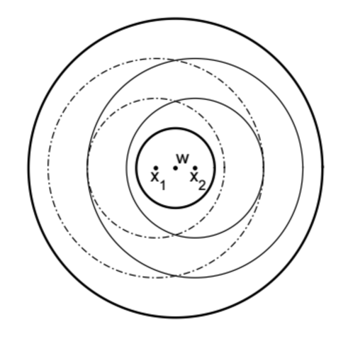
Figure 1. An annulus centered at $x_{1}$ and its translation centered at $x_{2}$ (marked with solid and dash-dot markers, resp.) are both subsets of a larger annulus (marked with thick marker) centered at the midpoint $w=(x_{1}+x_{2})/2.$ The larger annulus is a common superannulus of the two smaller annuli.

Proposition 2.2.

Let $0<a<b$ and $\tau\geq 2.$ If $x_{1},x_{2}\in{\mathbb{R}}^{n},|x_{1}-x_{2}|<a,$ and $w=(x_{1}+x_{2})/2$, then for $j=1,2$

$$R(x_{j},b,a)\subset R(w,d,c),\quad\frac{d}{c}\leq\frac{b}{a}\frac{1+|x_{1}-x_{2}|/b}{1-|x_{1}-x_{2}|/a}\,,$$

where $c=a-|x_{1}-x_{2}|,d=b+|x_{1}-x_{2}|\,.$ In particular, if $|x_{1}-x_{2}|<a/\tau^{2}$, then for $j=1,2$

$$R(x_{j},\tau b,a/\tau)\subset R(w,\tau^{2}b,a/\tau^{2}).$$

Moreover, $R(w,\tau^{2}b,a/\tau^{2})\subset B^{n}(x_{j},2\tau^{2}b),$ for $j=1,2.$

Proof.

The claims follow from the triangle inequality and we prove here only the second one. Without loss of generality we may assume that $j=1.$ Fix $u\in R(x_{1},\tau b,a/\tau).$ Then $\tau b>|u-x_{1}|>a/\tau$ and

$$|u-w|\geq|u-x_{1}+x_{1}-w|\geq|u-x_{1}|-|x_{1}-w|\geq a/\tau-a/\tau^{2}\geq a/\tau^{2}$$

where the last inequality holds because $\tau\geq 2.$ Similarly,

$$|u-w|\leq|u-x_{1}+x_{1}-w|\leq|u-x_{1}|+|x_{1}-w|\leq\tau b+a/\tau^{2}\leq\tau^{2}b$$

because $\tau\geq 2.$ Therefore $a/\tau^{2}\leq|u-w|\leq\tau^{2}b$ and hence $u\in R(w,\tau^{2}b,a/\tau^{2}).$ The last assertion also follows easily from the triangle inequality. ∎

Topology in ${\mathbb{R}}^{n}$ or in its one point compactification $\overline{{\mathbb{R}}}^{n}={\mathbb{R}}^{n}\cup\{\infty\}$ is the metric topology defined by the chordal metric. The chordal (spherical) metric is the function $q:\overline{{\mathbb{R}}}^{n}\times\overline{{\mathbb{R}}}^{n}\to[0,1],$

$$q(x,y) =\frac{|x-y|}{\sqrt{1+|x|^{2}}\sqrt{1+|y|^{2}}},\text{ if }x\neq\infty\neq y,\quad q(x,\infty)=\frac{1}{\sqrt{1+|x|^{2}}}.$$

Thus, for instance, an unbounded domain $G\subset{\mathbb{R}}^{n}$ has $\infty$ as one of its boundary points.

For the sake of convenient reference we record the following simple inequality.

Proposition 2.3.

For $a>0$ and $p\geq 1$ the inequality

$$t-a\geq\lambda^{p}\sqrt{1+t},\quad\lambda>1,$$

holds for all $t\geq\lambda^{2p}+\lambda^{p}\sqrt{1+a}+a.$

Proof.

The inequality clearly holds for all large values of $t,$ larger than $|x|,$ where $x$ is a root of $(x-a)^{2}-\lambda^{2p}(x+1)=0.$ By the quadratic formula we see that both roots have absolute value less than $\lambda^{2p}+\lambda^{p}\sqrt{1+a}+a.$ ∎

For two points in a domain, the next result gives an estimate for the number of annular domains separating these points. This result has an important role in the proof of one of our main results in Section 7.

Proposition 2.4.

Let $G\subset{\mathbb{R}}^{n}$ be a domain, let $E$ be a compact subset of $G\,,$ and choose $x,y\in E$ such that $d(x,\partial G)=d(E,\partial G)$ and $|x-y|\geq d(E)/2$. Fix $z_{0}\in\partial G$ so that $|x-z_{0}|=d(x,\partial G)$ and let $w=(x+z_{0})/2\,,\lambda>1$. If $d(E)/d(E,\partial G)>\lambda^{p}+2$ for some integer $p\geq 1,$ then there are $p$ disjoint annular domains

$$B^{n}(w,\lambda^{m}d(x,\partial G)/2)\setminus\overline{B}^{n}(w,\lambda^{m-1}d(x,\partial G)/2),\quad m=1,...,p$$

separating $x$ and $y$. Moreover, for $d(E)/d(E,\partial G)>\max\{\lambda^{p}+2,\lambda^{2}+2\lambda+2\},$ we have

$$p>c\log(1+d(E)/d(E,\partial G)),\quad c=1/(2\log\lambda).$$

Proof.

Because $\overline{B}^{n}(w,\lambda^{p}d(x,\partial G)/2)$ contains the largest annulus, it is enough to show that $|w-y|>\lambda^{p}d(x,\partial G)/2$. By the triangle inequality,

$$|y-w|\geq|x-y|-|x-w|\quad\Leftrightarrow\quad\frac{|y-w|}{|x-w|}\geq\frac{|x-y|}{|x-w|}-1\,.$$

Further,

$$|y-w|\geq\left(\frac{|x-y|}{|x-w|}-1\right)|x-w|\geq(\frac{d(E)}{d(E,\partial G)}-1)d(x,\partial G)/2\geq(\lambda^{p}+1)d(x,\partial G)/2\,$$

as desired. To prove the second claim, the lower bound for $p,$ fix an integer $p\geq 1$ with

$$\lambda^{p+1}+2\geq u>\lambda^{p}+2,\quad u=d(E)/d(E,\partial G).$$

Then

$$p+1\geq\frac{\log(u-2)}{\log\lambda}$$

holds. To find a lower bound for $p,$ we observe that the inequality

(2.5) $$p+1\geq\frac{\log(u-2)}{\log\lambda}>\frac{\log(1+u)}{2\log\lambda}+1$$

holds iff

$$\left(\frac{u-2}{\lambda}\right)^{2}>1+u\Leftrightarrow u^{2}-(4+\lambda^{2})u+4-\lambda^{2}>0.$$

By Proposition 2.3, this holds for all $u>\lambda^{2}+2\lambda+2.$ By (2.5), we see that this yields also the desired lower bound for $p.$ ∎

2.6.

Quasiconformal maps and moduli of curve families. Quasiconformal homeomorphisms $f:G\to G^{\prime}=f(G)$ between domains $G,G^{\prime}\subset{\mathbb{R}}^{n}$ are commonly defined in terms of moduli of curve families. For the basic properties of the modulus $\mathsf{M}(\Gamma)$ of a curve family $\Gamma$, the reader is referred to [2, 13, 11], [31, 6.1, p. 16], [12]. According to Väisälä’s book [31], $K$-quasiconformal maps are characterized by the inequality

$$\mathsf{M}(f\Gamma)/K\leq\mathsf{M}(\Gamma)\leq K\mathsf{M}(f\Gamma)$$

for every family of curves $\Gamma$ in $G$ where $f(\Gamma)=\{f(\gamma):\gamma\in\Gamma\}\,.$

The following monotonicity of the moduli of curve families is quite useful in various estimates. Let $\Gamma_{1},\Gamma_{2}$ be two curve families in ${\overline{\mathbb{R}}^{n}}$. We say that $\Gamma_{2}$ is minorized by $\Gamma_{1}$ and write $\Gamma_{2}>\Gamma_{1}$ for it, if every curve $\gamma\in\Gamma_{2}$ has a subcurve belonging to $\Gamma_{1}$. For instance, $\Gamma_{2}>\Gamma_{1}$ if $\Gamma_{2}\subset\Gamma_{1}.$

Lemma 2.7 ([31, §6]).

1. If $\Gamma_{2}>\Gamma_{1},$ then $\mathsf{M}(\Gamma_{2})\leq\mathsf{M}(\Gamma_{1})$.

2. For a collection of curve families $\Gamma_{i}~{}(i=1,2,\dots,N),$

   $$\mathsf{M}\left(\bigcup_{j}\Gamma_{i}\right)\leq\sum_{i=1}^{N}\mathsf{M}(\Gamma_{i}).$$

   Moreover, equality holds if the curve families are separate.

Here the families $\Gamma_{i}$ are said to be separate if they are contained in pairwise disjoint Borel sets $E_{i}$ (see also [11, §4.2.2]).

Let $G$ be a domain in ${\overline{\mathbb{R}}^{n}}$ and $E,F\subset\overline{G}.$ In what follows, $\Delta(E,F;G)$ will stand for the family of all the curves that are in $G$ except for the endpoints, and that have one endpoint in the set $E$ and another endpoint in $F$ [31, pp. 11-25], [12]. When $G=\mathbb{R}^{n}$ or $G=\overline{\mathbb{R}}^{n},$ we often write $\Delta(E,F;G)=\Delta(E,F).$

Lemma 2.8.

[31, Thm 7.5, p. 22] If $0<a<b$ and $D=\overline{B}^{n}(b)\backslash B^{n}(a)$,

$$\mathsf{M}(\Delta(S^{n-1}(a),S^{n-1}(b);D))=\omega_{n-1}(\log({b}/{a}))^{1-n},$$

where $\omega_{n-1}$ is the $(n-1)$-dimensional surface area of the unit sphere $S^{n-1}$.

Corollary 2.9.

Let $0<a<b$ and $E,F\subset D\equiv\overline{B}^{n}(b)\backslash B^{n}(a)$, and let

$$\mathsf{M}(\Delta(E,F;{\mathbb{R}}^{n}))\geq c>0.$$

Then there exists $\lambda=\lambda(n,c)>1$ such that for all $t\geq\lambda$

$$\mathsf{M}(\widetilde{\Delta})\geq c/2,\quad\widetilde{\Delta}=\Delta(E,F;B^{n}(0,tb)\setminus B^{n}(0,a/t)).$$

Proof.

By the subadditivity of the modulus, Lemma 2.7,

$$\mathsf{M}(\Delta(E,F;{\mathbb{R}}^{n}))\leq\mathsf{M}(\widetilde{\Delta})+\mathsf{M}(\Delta(E,F;{\mathbb{R}}^{n})\setminus\widetilde{\Delta})$$

whereas by Lemma 2.8

$$\mathsf{M}(\Delta(E,F;{\mathbb{R}}^{n})\setminus\widetilde{\Delta})\leq 2\omega_{n-1}(\log t)^{1-n}\leq c/2$$

for all $t\geq\lambda\equiv{\rm exp}((4\omega_{n-1}/c)^{1/(n-1)})>1.$ ∎

The Teichmüller ring is a domain in $\mathbb{R}^{n}$ with the complementary components $[-e_{1},0]$ and $[se_{1},\infty],s>0.$ The modulus of the family of all curves joining these boundary components, denoted by $\tau_{n}(s),$ is a decreasing homeomorphism $\tau_{n}:(0,\infty)\to(0,\infty)$ and admits the following lower bound

(2.10) $$\tau_{n}(s)\geq c_{n}\log\left(1+\frac{2(1+\sqrt{1+s})}{s}\right)\geq 2c_{n}\log(1+\frac{1}{\sqrt{s}})\,,\quad c_{n}=B(\frac{1}{2(n-1)},\frac{1}{2})^{1-n}\omega_{n-2},$$

where $B(\cdot,\cdot)$ is the beta function, $c_{2}=2/\pi$ [12, p.114]. For $n=2,$ $\tau_{2}$ can be expressed explicitly in terms of complete elliptic integrals [12, p. 123].

The function $\tau_{n}$ often occurs as a lower bound for moduli of curve families like in the following lemma, based on the spherical symmetrization of condensers. This lemma has found many applications because it provides, for a pair of non-degenerate continua $E$ and $F,$ an explicit connection between the geometric quantity $d(E,F)/\min\{d(E),d(F)\}$ and the modulus of the family of all curves joining the continua. Also a similar upper bound holds [32, 7.42], [12, Rmk 9.30], but the upper bound will not be needed here.

Lemma 2.11.

Let $E$ and $F$ be continua in $\mathbb{B}^{n}$ with $d(E),d(F)>0.$ Then

Proof.

If $d(E;F)=0,$ then $\mathsf{M}(\Delta(E,F;\mathbb{B}^{n}))=\mathsf{M}(\Delta(E,F;\mathbb{R}^{n}))=\infty$ by [12, 7.22] (or [32, 5.33]). If $d(E;F)>0,$ the proof of(1) follows from [12, Lemma 9.26] (or [32, 7.38]) and the proof of (2) from (1) and [12, Lemma 7.14] (or [32, 5.22]).

∎

2.12.

Quasiconformal self-homeomorphism of a domain. For a proper subdomain $G$ of ${\mathbb{R}}^{n}$ and for a fixed point $x\in G$, we define a homeomorphism $f:{\mathbb{R}}^{n}\to{\mathbb{R}}^{n}$ such that $f(z)=z$ if $z=x$ or $|x-z|\geq d(x,\partial G)$. Furthermore, for $0<{\alpha}<\beta<1$, the mapping $f$ fulfills $f(S^{n-1}(x,{\alpha}d(x,\partial G)))=S^{n-1}(x,\beta\,d(x,\partial G))$.

Let $h:{\mathbb{R}}^{n}\to{\mathbb{R}}^{n}$ be the radial map $x\mapsto|x|^{a-1}x=h(x)$, $a\neq 0$, defined in [31, 16.2, p. 49]. Suppose $0<{\alpha},{\beta}<1$ and we want to choose $a$ so that $h(S^{n-1}({\alpha}))=S^{n-1}({\beta})$. Then

(2.13) $${\alpha}^{a}={\beta}\quad\Leftrightarrow\quad a=\frac{\log({\beta})}{\log({\alpha})}$$

and, as shown in [31, 16.2], the maximal dilatation of this map is $K(h)=\max\{a^{n-1},a^{1-n}\}$. By definition, $h(z)=z$ for $z\in\{0\}\cup S^{n-1}$. Define now a function $g$ such that $g(z)=h(z)$ for all $z\in\overline{\mathbb{B}}^{n}$ but $g(z)=z$ whenever $|z|\geq 1$. By [31, Thm 35.1, p. 118], the dilatation of the mapping $g$ is same as the one of $h$.

Fix now $x$ in $G$ and let $r=d(x,\partial G)$. Let $f$ be a radial $K$-quasiconformal map defined by $f(z)=rg((z-x)/r)$, $z\in{\mathbb{R}}^{n}$. Then $f(x)=x$, $f(z)=z$ for all $z\in G\backslash B^{n}(x,r)$ and $f(B^{n}(x,{\alpha}\,r))=B^{n}(x,{\beta}\,r)$, similarly as above.

We summarize the above arguments as a lemma.

Lemma 2.14.

For a proper subdomain $G$ of ${\mathbb{R}}^{n}$ and for a fixed point $x\in G$, there exists a quasiconformal homeomorphism $f:{\mathbb{R}}^{n}\to{\mathbb{R}}^{n}$ such that $f(G)=G,$ and $f(z)=z$ if $z=x$ or $|x-z|\geq d(x,\partial G)$. Furthermore, for $0<{\alpha}<\beta<1$,

$$f(S^{n-1}(x,{\alpha}d(x,\partial G)))=S^{n-1}(x,\beta\,d(x,\partial G)),\quad K(f)=\max\{a^{n-1},a^{1-n}\},$$

where $a$ is the number in (2.13).

3. Harnack inequality and capacity test functions

In the dimensions $n\geq 3$, quasihyperbolic distances defined below are widely used as substitutes of hyperbolic distances.

3.1.

Quasihyperbolic metric. For a domain $G\subsetneq{\mathbb{R}^{n}}$, the quasihyperbolic metric ${k}_{G}$ is defined by [11, p. 39], [12, p.68]

$${k}_{G}(x,y)=\inf_{\gamma\in\Gamma}\int_{\gamma}\frac{|dz|}{d(z,\partial G)},\quad x,y\in G,$$

where $\Gamma$ is the family of all rectifiable curves in $G$ joining $x$ and $y$. This infimum is attained when $\gamma$ is the quasihyperbolic geodesic segment joining $x$ and $y\,.$ The hyperbolic metric of $\mathbb{B}^{n}$ can be also defined in terms of a similar length minimizing property, with the weight function $2/(1-|x|^{2})\,.$ In many ways the quasihyperbolic metric is similar to the hyperbolic metric, see [12, Chapter 5], but unfortunately its values are known only in a few special cases. Fortunately, some lower bounds can be given in terms of the $j_{G}$ metric and upper bounds can be given for a large class of domains as we will now show.

The distance ratio metric is defined in a domain $G\subsetneq{\mathbb{R}}^{n}$ as the function $j_{G}:G\times G\to[0,\infty)$,

$$j_{G}(x,y)=\log(1+\frac{|x-y|}{\min\{d(x,\partial G),d(y,\partial G)\}}).$$

The lower bound

$$j_{G}(x,y)\leq k_{G}(x,y)$$

holds for an arbitrary $G\subsetneq{\mathbb{R}^{n}}$ and all $x,y\in G$ [12, Cor. 5.6, p.69].

For the upper bound we introduce a class of domains for which we have a simple upper bound of the quasihyperbolic distance. This upper bound combined with the above lower bound provide handy estimates for many applications.

3.2.

$\varphi$- uniform domains. We say that a domain $G$ is $\varphi$-uniform if for all $x,y\in G$

$$k_{G}(x,y)\leq\varphi(|x-y|/\min\{d(x,\partial G),d(y,\partial G)\})\,.$$

The special case $\varphi(t)=c\log(1+t),c>1\,,$ yields the so called uniform domains which are ubiquitous in geometric function theory [12, p.84], [13]. For instance, balls and half-spaces and their images under quasiconformal mappings of $\mathbb{R}^{n}$ belong to this class of domains. It is easy to check that all convex domains are $\varphi$-uniform with $\varphi(t)\equiv t\,.$ The strip domain $\{z\in\mathbb{C}:0<{\rm Im}z<1\}$ is $\varphi$-uniform but not uniform.

3.3.

Harnack functions [12, p. 96]. Let $G\subset\mathbb{R}^{n}$ be a domain and let $u:G\to(0,\infty)$ be a continuous function. We say that $u$ is a Harnack function with parameters $(s,C),0<s<1<C,$ if for every $z\in G$ and all $x\in\overline{B}^{n}(z,sd(z,\partial G))$

$$u(z)\leq Cu(x)\,.$$

It follows easily from the definition of the quasihyperbolic metric, see [12, p. 69, Lemma 5.7], that the balls $\overline{B}^{n}(z,sd(z,\partial G))$ in the definition of a Harnack function have quasihyperbolic diameters majorized by a constant depending on $s$ only. For given $x,y\in G$ one can now estimate for a Harnack function $u$ the quotient $u(x)/u(y)$ using the quasihyperbolic distance $k_{G}(x,y)$ in a simple way as shown in [12, pp.94-95]. In fact, we fix a quasihyperbolic geodesic in $G$ joining $x$ and $y$ [12, p. 68, Lemma 5.1], and cover it optimally, using as few balls $\overline{B}^{n}(z,sd(z,\partial G))$ as possible. In this way, we obtain the next lemma.

Lemma 3.4.

[12, Lemma 6.23, p.96] Let $u:G\to(0,\infty)$ be a Harnack function with parameters $(s,C)\,.$

(1) Then

$$u(x)\leq C^{1+t}\,u(y)\,,\quad t=k_{G}(x,y)/d_{1}(s)\,,$$

for $x,y\in G$ where $d_{1}(s)=2\log(1+s)\,.$

(2) If a domain $G\subset\mathbb{B}^{n},0\in G\,,$ is $\varphi$-uniform, then for $d(y,\partial G)<d(0,\partial G)$

$$u(y)/u(0)>C^{-1-\varphi(2/d(y,\partial G))/d_{1}(s)}\,.$$

We next start our study of the capacity test function

(3.5) $$u_{\alpha}(z)=\mathrm{cap}\,(G,\overline{B}^{n}(z,\alpha d(z,\partial G)))\,,\quad\alpha\in(0,1)\,.$$

and examine its dependence on $\alpha$ and $z$ when the other argument is fixed. It turns out that the dependence of the capacity test function on $\alpha$ is controlled by standard ring domain capacity estimates from 2.12 whereas, as a function of $z,$ it is continuous and satisfies a Harnack condition.

Lemma 3.6.

Let $G\subset{\mathbb{R}}^{n}$, $x\in G\,,$ $0<{\alpha}<{\beta}<1\,,$ and $a=\log({\beta})/\log({\alpha})$. Then

$$\mathsf{M}(\Gamma_{\alpha})\leq\mathsf{M}(\Gamma_{\beta})\leq a^{n-1}\,\mathsf{M}(\Gamma_{\alpha}),$$

where $\Gamma_{s}=\Delta(S^{n-1}(x,sd(x,\partial G)),\partial G;G)$ for $s={\alpha},{\beta}$. In other words,

$$u_{\alpha}(x)\leq u_{\beta}(x)\leq a^{n-1}u_{\alpha}(x)\,.$$

Proof.

The first inequality follows from Lemma 2.7 and, by using the quasiconformal map $f$ of 2.12, we see that the second inequality holds. ∎

The above result shows that for a fixed $x\in G,$ $u_{\alpha}(x)$ is continuous with respect to the parameter $\alpha$ because $a\to 1$ when $\beta\to\alpha\,.$ The next result shows, among other things, that for a fixed $\alpha\in(0,1),$ $u_{\alpha}(x)$ is continuous as a function of $x\,.$ This continuity follows from the domain monotonicity of the capacity (4.4) and Lemma 3.6.

Theorem 3.7.

Let $G$ be a domain in ${\mathbb{R}}^{n}$ with boundary of positive capacity. Let $\alpha\in(0,1)$ and choose $s\in(0,1)$ so small that $(1+s)\alpha+s<1.$ The capacity test function $u_{\alpha}$ of $G$ is continuous on $G$ and satisfies the Harnack inequality with parameters $(s,C),$ where

$$C=\left(\frac{\log((1+s)\alpha+s)}{\log\alpha}\right)^{n-1}.$$

Proof.

For $z\in G$, we take $x\in\overline{B}^{n}(z,s\,d(z,\partial G))\,;$ namely,

(3.8) $$|x-z|\leq s\,d(z,\partial G).$$

It follows from the triangle inequality and the inequality (3.8) that

(3.9) $$d(x,\partial G)\leq|x-z|+d(z,\partial G)\leq(1+s)d(z,\partial G)\,,$$

(3.10) $$(1-s)d(z,\partial G)\leq d(z,\partial G)-|x-z|\leq d(x,\partial G)\,.$$

Note here that $\overline{B}^{n}(a,r_{a})\subset\overline{B}^{n}(b,r_{b})$ if and only if $|a-b|+r_{a}\leq r_{b}$. By using the inequalities (3.8) and (3.9), we have

$$|x-z|+\alpha d(x,\partial G)\leq s\,d(z,\partial G)+(1+s)\alpha\,d(z,\partial G)=((1+s)\alpha+s)\,d(z,\partial G)\,.$$

Similarly, by the inequalities (3.8) and (3.10),

$$|x-z|+\alpha d(z,\partial G))\leq(s+\alpha)d(z,\partial G)\leq\frac{s+\alpha}{1-s}d(x,\partial G)\,.$$

Therefore, we have

$$\overline{B}^{n}(x,\alpha\,d(x,\partial G))\subset\overline{B}^{n}(z,((1+s)\alpha+s)d(z,\partial G))\,,$$

$$\overline{B}^{n}(z,\alpha\,d(z,\partial G))\subset\overline{B}^{n}(x,\beta\,d(x,\partial G))\,,$$

where $\beta=(\alpha+s)/(1-s)\,.$ In particular, with the help of Lemma 3.6, we obtain

$$u_{\alpha}(x) \leq u_{(1+s)\alpha+s}(z)\leq Cu_{\alpha}(z)\,,$$

$$u_{\alpha}(z) \leq u_{\beta}(x)\leq Du_{\alpha}(x),$$

where $D=[\log\beta/\log\alpha]^{n-1}.$ The first inequality is nothing but the required Harnack inequality. Since $C<D,$ we obtain

$$|u_{\alpha}(z)-u_{\alpha}(x)|\leq D=\left(\frac{\log[(\alpha+s)/(1-s)]}{\log\alpha}\right)^{n-1}.$$

Now the continuity of $u_{\alpha}$ follows because $D\to 1$ as $s\to 0.$ ∎

Let $G\subset{\mathbb{R}}^{n}$ be a domain with $\mathrm{cap}\,(\partial G)>0,z_{1}\in G$ and fix $\alpha=1/4\,.$ Theorem 3.7 and Lemma 3.4 show that, perhaps surprisingly, the speed of decrease of the function $u_{\alpha}(z)/u_{\alpha}(z_{1})$ to $0$ when $k_{G}(z_{1},z)\to\infty$ or $z\to\partial G$ is controlled from below by the Harnack parameters given by Theorem 3.7 and by $k_{G}(z_{1},z)\,.$

4. Capacity test function

Various capacities are widely applied in geometric function theory to investigate the metric size of sets [10, 9]. We use here the conformal capacity of condensers and prove several lemmas involving this capacity. We begin by pointing out the connection between condenser capacity the modulus of a curve family. These lemmas, together with the superannulus Proposition 2.2, are applied to prove Lemma 4.8, which will be a key tool for the proof of a main result in Section 7.

A domain $D\subset\overline{{\mathbb{R}}}^{n}$ is called a ring if its complement $\overline{{\mathbb{R}}}^{n}\backslash D$ has exactly two components $C_{0}$ and $C_{1}$. Sometimes, we write $D=R(C_{0},C_{1}).$ We say that a ring $D=R(C_{0},C_{1})$ separates a set $E$, if $E\subset C_{0}\cup C_{1}$ and if $E$ meets both of $C_{0}$ and $C_{1}.$ As in [12, 7.16, p. 120], the (conformal) modulus of a ring $D=R(C_{0},C_{1})$ is defined by

$${\rm mod}(D)=\left(\frac{\mathsf{M}(\Delta(C_{0},C_{1}))}{\omega_{n-1}}\right)^{1/(1-n)}$$

and its capacity is $\mathrm{cap}\,(D)=\mathsf{M}(\Delta(C_{0},C_{1}))$.

Definition 4.1.

[12, Def. 9.2, p. 150] A pair $E=(A,C)$ where $A\subset{\mathbb{R}}^{n}$ is open and non-empty, and $C\subset A$ is compact and non-empty is called a condenser. The capacity of this condenser $E$ is

$${\rm cap}(E)=\inf_{u}\int_{{\mathbb{R}}^{n}}|\nabla u|^{n}dm,$$

where the infimum is taken over the family of all non-negative $\text{ACL}^{n}$ functions $u$ with compact support in $A$ such that $u(x)\geq 1$ for $x\in C$. A compact set $E$ is of capacity zero, denoted by $\mathrm{cap}\,E=0\,,$ if $\mathrm{cap}\,(A,C)=0\,$ for some bounded domain $A,C\subset A\,.$ Otherwise we denote $\mathrm{cap}\,E>0\,$ and say that $E$ is of positive capacity. Note that the definition of capacity zero does not depend on the open bounded set $A$ [12, pp.150-153].

For the definition of ACL and $\text{ACL}^{n}$ mappings, see [31, Def. 26.2, p. 88; Def. 26.5 p. 89], [11, 6.4]. It is useful to recall the close connection between the modulus of a curve family and capacity, because many properties of curve families yield similar properties for the capacity.

Remark 4.2.

[11, p.164, Thm 5.2.3], [12, Thm 9.6, p. 152] The capacity of a condenser $E=(A,C)$ can also be expressed in terms of a modulus of a curve family as follows:

$${\rm cap}(E)=\mathsf{M}(\Delta(C,\partial A;A))\,.$$

Lemma 4.3.

Let $E\subset{\mathbb{R}}^{n}$ be a compact set, $x\in{\mathbb{R}}^{n},$ and let $0<r<s<t.$ Then

$$A\geq{\mathrm{cap}\,}(B^{n}(x,t),E\cap\overline{B}^{n}(x,r))\geq\left(\frac{\log(s/r)}{\log(t/r)}\right)^{n-1}A,\quad A\equiv{\mathrm{cap}\,}(B^{n}(x,s),E\cap\overline{B}^{n}(x,r)).$$

Proof.

The proof follows immediately from Remark 4.2 and Lemma 2.14. ∎

Let $E=(A,C)$ be a condenser and $A_{1}$ a domain with $A\subset A_{1}\,.$ It follows readily from the definition of the capacity (and also from Lemma 2.7) that the following domain monotonicity property holds

(4.4) $$\mathrm{cap}\,(A_{1},C)\leq\mathrm{cap}\,(A,C)\,.$$

For a compact set $E\subset{\mathbb{R}}^{n}$ , $x\in{\mathbb{R}}^{n},$ and $r>0,$ we introduce the notation

(4.5) $${\rm cap}(x,E,r)=\mathsf{M}(\Delta(x,E,r))\,,\quad\Delta(x,E,r)=\Delta(S^{n-1}(x,2r),E\cap\overline{B}^{n}(x,r);{\mathbb{R}}^{n})\,.$$

The condition ${\rm cap}(x,E,r)>0$ gives information about the size of the set $E$ in a neighborhood of the point $x.$ The next lemma shows that there is a substantial part of the set $E,$ in the sense of capacity, in an annulus centered at $x.$

Lemma 4.6.

Let $E\subset{\mathbb{R}}^{n}$ be a compact set, $x\in{\mathbb{R}}^{n},$ and $r>0$ and suppose that

$$\mathsf{M}(\Delta(x,E,r))=c>0.$$

If $\Delta_{1}=\Delta(S^{n-1}(x,2r),E\cap\overline{B}^{n}(x,r);B^{n}(x,2r)),$ then

$$\mathsf{M}(\Delta(x,E,r))=\mathsf{M}(\Delta_{1}).$$

Fix $\lambda=\lambda(n,c)=\max\{t,2\},$ where $t>1$ satisfies

$$\omega_{n-1}(\log 2t)^{1-n}=c/2\,,$$

and, for $\sigma>1,let$

$$\widetilde{\Delta}(x,E,r,\sigma)=\Delta(S^{n-1}(x,2r),E\cap(\overline{B}^{n}(x,r)\setminus{B}^{n}(x,r/\sigma)):\overline{B}^{n}(x,2r)\setminus{B}^{n}(x,r/\sigma)).$$

Then for every $\sigma\geq\lambda,$

$$\mathsf{M}(\widetilde{\Delta}(x,E,r,\sigma))\geq c/2.$$

Proof.

The equality $\mathsf{M}(\Delta(x,E,r))=\mathsf{M}(\Delta_{1})$ is a basic property of the modulus, see [31, p.33, Thm 11.3]. By the subadditivity of the modulus in Lemma 2.7,

$$\mathsf{M}(\Delta(x,E,r))=\mathsf{M}(\Delta_{1})\leq\mathsf{M}(\widetilde{\Delta}(x,E,r,\sigma))+\mathsf{M}(\Delta_{1}\setminus\widetilde{\Delta}(x,E,r,\sigma))$$

and, by the choice of $\lambda$ and Lemmas 2.7 and 2.8,

$$\mathsf{M}(\Delta_{1}\setminus\widetilde{\Delta}(x,E,r,\sigma))\leq c/2$$

for all $\sigma\geq\lambda.$ Finally,

$$\mathsf{M}(\widetilde{\Delta}(x,E,r,\sigma))\geq\mathsf{M}(\Delta_{1})-\mathsf{M}(\Delta_{1}\setminus\widetilde{\Delta}(x,E,r,\sigma))\geq c-c/2=c/2.$$

∎

According to Lemma 4.6 we can find, under the above assumptions, a substantial portion of the set $E$ in the annulus $\overline{B}^{n}(x,r)\setminus B^{n}(x,r/\lambda)$ for $x\in E.$ We need to use this type of annuli for two disjoint sets $E$ and $F$, which are close enough to each other and then to find a lower bound for the modulus of the curve family joining the respective substantial portions of each set. These annuli are translated versions of each other and we can use Proposition 2.2 to find a common superannulus for both annuli and consider the joining curves in this superannulus. To quantify this idea, we need a comparison principle of the modulus of a curve family from [32, p.61 Lemma. 5.35] , [11, p.182, Thm 5.5.1].

Lemma 4.7.

(1) [32, p.61 Lemma. 5.35] Let $G$ be a domain in $\overline{{\mathbb{R}}}^{n}$, let $F_{j}\subset G$, $j=1,2,3,4$, and let $\Gamma_{ij}=\Delta(F_{i},F_{j};G)$, $1\leq i,j\leq 4$. Then

$$\mathsf{M}(\Gamma_{12})\geq 3^{-n}\min\{\,\mathsf{M}(\Gamma_{13}),\;\mathsf{M}(\Gamma_{24}),\;\inf\mathsf{M}\bigl{(}\Delta(|\gamma_{13}|,|\gamma_{24}|;G)\bigr{)}\,\}\;,$$

where the infimum is taken over all rectifiable curves $\gamma_{13}\in\Gamma_{13}$ and $\gamma_{24}\in\Gamma_{24}$.

(2) [32, p.63, 5.41 and 5.42] If $F_{j}\subset B^{n}(z,s)\subset G,j=1,2,3,4,$ and and there exists $t>0$ such that for all $\gamma_{13}\in\Gamma_{13}$ and $\gamma_{24}\in\Gamma_{24}$

$$d(|\gamma_{13}|)\geq ts,\quad d(|\gamma_{24}|)\geq ts,$$

then there is a constant $v=v(n,b/a,t)$ such that

$$\mathsf{M}(\Gamma_{12})\geq v\min\{\,\mathsf{M}(\Gamma_{13}),\;\mathsf{M}(\Gamma_{24})\;\}\;.$$

Proof.

The first claim (1) is proved in the cited reference. The second claim also follows easily from the cited reference but for clarity we include the details here. We apply the comparison principle of part (1) to get a lower bound for $\mathsf{M}(\Gamma_{12})$. Because $F_{j}\subset B^{n}(z,s)\subset G,j=1,2,3,4,$ it follows from Lemma 2.10 that the infimum in the lower bound of (1) is at least $v_{1}(n,t)\equiv\frac{1}{2}\tau_{n}(4m^{2}+4m),\,m=2/t,$ and thus

$$\mathsf{M}(\Gamma_{12})\geq 3^{-n}\min\{\,\mathsf{M}(\Gamma_{13}),\;\mathsf{M}(\Gamma_{23}),v_{1}(n,t)\}.$$

By Lemma 2.8

$$\max\bigl{\{}\,\mathsf{M}(\Gamma_{13}),\;\mathsf{M}(\Gamma_{23})\,\bigr{\}}\leq A\equiv\omega_{n-1}\Bigl{(}\log{b\over a}\Bigr{)}^{1-n}\;$$

and further

$$\mathsf{M}(\Gamma_{12}) \geq 3^{-n}\min\Bigl{\{}\,\mathsf{M}(\Gamma_{13}),\;\mathsf{M}(\Gamma_{23}),\;{1\over A}\Bigl{(}v_{1}(n,t)\Bigr{)}\min\bigr{\{}\,\mathsf{M}(\Gamma_{13}),\;\mathsf{M}(\Gamma_{23})\,\bigr{\}}\Bigr{\}}$$

$$\geq v(n,b/a,t)\min\bigl{\{}\,\mathsf{M}(\Gamma_{13}),\;\mathsf{M}(\Gamma_{23})\,\bigr{\}}$$

where $v(n,b/a,t)=3^{-n}\min\bigl{\{}\,1,\,{1\over A}v_{1}(n,t)\bigr{\}}$.

∎

The next lemma will be a key tool in Section 7. It is based on three earlier results:

• the superannulus Proposition 2.2,

• the substantial subset selection Lemma 4.6,

• the comparison principle for the modulus of a curve family, Lemma 4.7.

Recall the notation $R(x,r^{\prime},r)$ for $0<r<r^{\prime}<+\infty$ and $x\in{\mathbb{R}}^{n}$ from (2.1).

Lemma 4.8.

Let $n\geq 2,c>0$ and $\lambda=\lambda(n,c)\geq 2$ be as in Lemma 4.6. Let $E,F\subset{\mathbb{R}}^{n}$ be compact sets, $x,y\in{\mathbb{R}}^{n},$ and $r>0$ and suppose that

$$\mathsf{M}(\Delta(x,E,r))=c>0,\quad\mathsf{M}(\Delta(y,F,r))=c>0.$$

If $|x-y|<r/\lambda^{2},$ then there exist constants $\tau=\tau(n,c)\geq 2,d=d(n,c)>0$ such that with $w=(x+y)/2$

$$\mathsf{M}(\Delta(E,F;R(w,\tau^{2}r,r/\tau^{2})))\geq d.$$

Proof.

By Proposition 2.2, we see that

$$R(x,r,r/\lambda)\cup R(y,r,r/\lambda)\subset R(w,\lambda^{2}r,r/\lambda^{2})$$

and that $R(w,\lambda^{2}r,r/\lambda^{2})$ is a common superannulus for the two smaller annuli. We apply the comparison principle for the modulus, Lemma 4.7(2), with

$$F_{1}=E\cap R(x,r,r/\lambda),\quad F_{2}=F\cap R(y,r,r/\lambda),$$

$$F_{3}=S^{n-1}(x,2r),\quad F_{4}=S^{n-1}(y,2r).$$

Observe first that, in the notation of Lemma 4.7, for all $\gamma_{13}\in\Gamma_{13}$ and $\gamma_{24}\in\Gamma_{24}$

$$d(|\gamma_{13}|)\geq r,\quad d(|\gamma_{24}|)\geq r$$

and that, by Proposition 2.2, $F_{j}\subset R(w,2\lambda^{2}r,r/\lambda^{2})$ for $j=1,2,3,4.$ By Lemma 4.7(2), we have

$$\mathsf{M}(\Delta(F_{1},F_{2};{\mathbb{R}}^{n}))\geq d_{2}(n,c)>0.$$

Using Lemma 4.6 we obtain the numbers $d=d_{2}(n,c)/2$ and $\tau.$ ∎

5. Hausdorff content and lower estimate of capacity

In this section, we discuss lower bounds for the capacity in terms of the Hausdorff $h$-content. Our main references are O. Martio [19] and Yu.G. Reshetnyak [25], [26, pp.110-120]. Reshetnyak also cites an earlier lemma of H. Cartan 1928 and gives its proof based on the work of L.V. Ahlfors [1] (cf. R. Nevanlinna [22, p.141]). We give here a short review of the earlier relevant results and, for the reader’s benefit, outline sketchy proofs.

We start with the next covering lemma [17, p. 197]. In the following, we denote by $\chi_{E}$ the characteristic function of a set $E\subset{\mathbb{R}}^{n};$ that is, $\chi_{E}(x)=1$ if $x\in E$ and $\chi_{E}(x)=0$ otherwise.

Lemma 5.1.

Let $n$ be an integer with $n\geq 2$ and let $A$ be a set in ${\mathbb{R}}^{n}.$ Suppose that a radius $r(x)>0$ is assigned for each point $x\in A$ in such a way that $\sup_{x\in A}r(x)<+\infty.$ Then one can find a countable subset $\{x_{k}\}$ of $A$ such that

(5.2) $$\chi_{A}(x)\leq\sum_{k}\chi_{B_{k}}(x)\leq N_{n},\quad x\in{\mathbb{R}}^{n},$$

where $B_{k}=B^{n}(x_{k},r(x_{k}))$ and $N_{n}$ is a constant depending only on $n.$

The above inequalities mean that $A$ is covered by the family of balls $\{B_{k}\}$ and the number of overlapping of the covering is at most $N_{n}.$ It is an interesting problem to find the best possible number $N_{n}^{*}$ for the constant $N_{n}$ in the above lemma. For $\varphi\in(0,\pi],$ we will say that a subset $V$ of the unit sphere $S^{n-1}=\{x\in{\mathbb{R}}^{n}:|x|=1\}$ is $\varphi$-separated if the angle subtended by the two line segments $PO$ and $QO$ is at least $\varphi$ for distinct points $P,Q$ in $V.$ We denote by $\nu(n,\varphi)$ the maximal cardinal number of $\varphi$-separated subsets $V$ of $S^{n-1}.$ For instance, $\nu(n,\pi)=2.$ It is clear that $\nu(n,\varphi)\leq\nu(n,\varphi^{\prime})$ for $0<\varphi^{\prime}<\varphi.$ The proof of the above lemma in p. 199 of [17] tells us that

$$N_{n}^{*}\leq 1+\inf_{\varphi<\pi/3}\nu(n,\varphi).$$

On the other hand, a standard compactness argument leads to the left continuity of $\nu(n,\varphi)$; that is, $\nu(n,\varphi^{\prime})\to\nu(n,\varphi)$ as $\varphi^{\prime}\to\varphi^{-}.$ Hence, we have $N_{n}^{*}\leq 1+\nu(n,\pi/3).$ Here we note that the number $\nu(n,\pi/3)$ is known as the kissing number $\kappa(n)$ in dimension $n$ [8]. This number is closely related to other important issues such as sphere packing problems. For instance, it is known that $\kappa(2)=6,\kappa(3)=12,\kappa(4)=24.$ However, it is difficult to determine $\kappa(n)$ in general. The true value of $\kappa(5)$ is not determined up to the present. By using the special nature of the lattices $E_{8}$ and $\Lambda_{24},$ Viazovska determined $\kappa(8)$ and, later with her collaborators, $\kappa(24)$ and won a Fields medal in 2022 [23]. In summary, we can state the following.

Lemma 5.3.

The minimal number $N_{n}^{*}$ of the bound $N_{n}$ in Lemma 5.1 satisfies the inequality $N_{n}^{*}\leq\kappa(n)+1,$ where $\kappa(n)$ is the kissing number in dimension $n.$

Let $h(r)$ be a measure function, that is, a monotone increasing continuous function on $0<r<+\infty$ with $h(r)\to 0$ as $r\to 0$ and $h(r)\to+\infty$ as $r\to+\infty.$ The $h$-Hausdorff content of a set $E\subset{\mathbb{R}}^{n}$ is defined as

$$\Lambda_{h}(E)=\inf\left\{\sum_{k}h(r_{k}):E\subset\bigcup_{k}B^{n}(a_{k},r_{k})\right\}.$$

For a positive number $\beta>0,$ and for $h(r)=r^{\beta},$ the $h$-Hausdorff content is called the $\beta$-dimensional Hausdorff content and denoted by $\Lambda^{\beta}(E).$ Recall that the Hausdorff dimension $\dim E$ of $E$ is characterized as the infimum of $\beta>0$ with $\Lambda^{\beta}(E)=0.$

The next lemma constitutes a key step in the proof of Martio’s Theorem 5.7 below. In the proof below we give explicit estimates of the relevant constants.

Remark 5.4.

The next lemma has a long history which goes back to H. Cartan and L.V. Ahlfors [1], [22, p. 141]. Yu.G. Reshetnyak [25], [26, Lemma 3.7, p.115], extended their two dimensional work to the case of $\mathbb{R}^{n}$ and applied the result to prove a lower bound for the capacity in terms of the Hausdorff content. O. Martio, in turn, made use of these results in his paper [19] which is one of our key references.

Lemma 5.5 (Lemma 2.6 in [19]).

Let $\sigma$ be a positive finite measure on ${\mathbb{R}}^{n}$ and $h$ be a measure function. We denote by $T$ the set of those points $x\in{\mathbb{R}}^{n}$ for which the inequality $\sigma(B^{n}(x,r))\leq h(r)$ holds for all $r>0.$ Then $\Lambda_{h}({\mathbb{R}}^{n}\setminus T)\leq N_{n}^{*}\sigma({\mathbb{R}}^{n}),$ where $N_{n}^{*}$ is given in Lemma 5.3.

Proof. We choose $r_{0}>0$ so that $h(r_{0})=\sigma({\mathbb{R}}^{n})$ and let $A={\mathbb{R}}^{n}\setminus T.$ For each $x\in A,$ by definition, there is a positive $r(x)$ such that $\sigma(B^{n}(x,r(x)))>h(r(x)).$ Note that $r(x)\leq r_{0}.$ We now apply Lemma 5.1 to extract a countable set $\{x_{k}\}$ from $A$ so that $B_{k}=B^{n}(x_{k},r(x_{k}))$ satisfy (5.2). Then

$$\Lambda_{h}(A) \leq\sum_{k}h(r(x_{k}))<\sum_{k}\sigma(B_{k})$$

$$=\sum_{k}\int\chi_{B_{k}}d\sigma=\int\sum_{k}\chi_{B_{k}}d\sigma\leq N_{n}^{*}\sigma({\mathbb{R}}^{n}).$$

∎

By making use of the last lemma, Martio proved the following. For the proof, see Lemma 2.8 in [19].

Lemma 5.6.

Let $1<p\leq n$ and $\alpha>0.$ For a function $u\geq 0$ in $L^{p}({\mathbb{R}}^{n})$ with support in $B^{n}(0,r_{1}),$ the set $F$ of points $x\in{\mathbb{R}}^{n}$ satisfying the inequality

$$v(x):=\int_{{\mathbb{R}}^{n}}u(y)|x-y|^{1-n}dm(y)>\Omega_{n}^{1-1/p}\left(\frac{n-1}{\alpha}\int_{0}^{r_{1}}h(t)^{1/p}t^{-n/p}dt+r_{1}^{1-n/p}\|u\|_{p}\right)$$

admits the estimate $\Lambda_{h}(F)\leq N_{n}(\alpha\|u\|_{p})^{p},$ where $N_{n}$ is the number in Lemma 5.1.

Let

$$K_{n}=2^{-n}\omega_{n-1}^{n}\Omega_{n}^{1-n}=\frac{1}{\Gamma(\frac{n}{2}+1)}\left(\frac{n\sqrt{\pi}}{2}\right)^{n}.$$

The following theorem is a special case of Theorem 3.1 in [19] when $p=n.$ Since an explicit form of the constant $M_{1}$ is not given in [19], we give an outline of the proof with a concrete form of $M_{1}.$

Theorem 5.7.

Suppose that a measure function $h(r)$ satisfies the inequality

$$I(r)=\int_{0}^{2r}h(t)^{1/n}t^{-1}dt\leq Ah(r)^{1/n},\quad 0<r\leq r_{0},$$

for some constants $A>0$ and $r_{0}>0.$ Let $E$ be a closed set in ${\mathbb{R}}^{n}.$ Then

(5.8) $$\frac{\Lambda_{h}(E\cap{\overline{B}^{n}}(x,r))}{h(r)}\leq M_{1}\cdot\mathrm{cap}\,(x,E,r),\quad x\in{\mathbb{R}}^{n},~{}0<r\leq r_{0},$$

where $M_{1}$ is the positive constant given by

(5.9) $$M_{1}=\max\left\{2^{n}A^{n}\left(\frac{n-1}{n}\right)^{n}\,N_{n},1/K_{n}\right\}.$$

Proof. We may assume $x=0$ and write $B_{r}=B^{n}(0,r)$ for short. Because $E\cap B_{r}\subset B_{r^{\prime}},r<r^{\prime},$ by the definition of the Hausdorff content it is clear that $\Lambda_{h}(E\cap B_{r})\leq h(r).$ Since $M_{1}\geq 1/K_{n},$ the required inequality holds trivially when $\mathrm{cap}\,(0,E,r)\geq K_{n}.$ Thus we may assume that $\mathrm{cap}\,(0,E,r)<K_{n}.$ By the definition of capacity, for each $r>0$ and a small enough $\varepsilon>0,$ we may choose a smooth function $w\geq 0$ on ${\mathbb{R}}^{n}$ with support in $B_{2r}$ so that $w>1$ on $E\cap B_{r}$ and so that

$$\|\nabla w\|_{n}^{n}=\int_{{\mathbb{R}}^{n}}|\nabla w|^{n}dm<\mathrm{cap}\,(B_{2r},E\cap B_{r})+\varepsilon=\mathrm{cap}\,(0,E,r)+\varepsilon<K_{n},$$

where $dm$ denotes the Lebesgue measure.

We apply Lemma 5.6 with $r_{1}=2r$ and $p=n$ to the function $u=|\nabla w|/\omega_{n-1}$ and by the above inequality we may choose $\alpha$ so that

$$\Omega_{n}^{1-1/n}\left(\frac{n-1}{\alpha}I(r)+\frac{\|\nabla w\|_{n}}{\omega_{n-1}}\right)=1.$$

Since $\|\nabla w\|_{n}<K_{n}^{1/n},$ we have the inequality $\|\nabla w\|_{n}/\omega_{n-1}<\Omega_{n}^{1/n-1}/2,$ which enables us to estimate $\alpha$ as

$$\alpha=\frac{(n-1)I(r)}{\Omega_{n}^{1/n-1}-\|u\|_{n}}<\frac{2(n-1)I(r)}{\Omega_{n}^{1/n-1}}\leq 2A(n-1)\Omega_{n}^{1-1/n}h(r)^{1/n}$$

for $0<r\leq r_{0}.$ By the representation formula (see [19, (2.2)])

$$w(x)=\frac{1}{\omega_{n-1}}\int_{{\mathbb{R}}^{n}}\frac{\nabla w(y)\cdot(x-y)}{|x-y|^{n}}dm(y),$$

we have the inequality

$$w(x)\leq\frac{1}{\omega_{n-1}}\int_{{\mathbb{R}}^{n}}\frac{|\nabla w(y)||x-y|}{|x-y|^{n}}dm(y)=\int_{{\mathbb{R}}^{n}}u(y)|x-y|^{1-n}dm(y)=v(x).$$

Let $F$ be as in Lemma 5.6. In particular, we have $E\cap B_{r}\subset F$ and thus by Lemma 5.6

$$\Lambda_{h}(E\cap B_{r})\leq\Lambda_{h}(F)\leq N_{n}(\alpha\|u\|_{n})^{n}\leq N_{n}\,d_{n}\,h(r)(\mathrm{cap}\,(0,E,r)+\varepsilon)\,,$$

where

$$d_{n}=\frac{2^{n}A^{n}(n-1)^{n}}{n\Omega_{n}}\left(\frac{\Omega_{n}}{\omega_{n-1}}\right)^{n-1}=2^{n}A^{n}(\frac{n-1}{n})^{n}.$$

Letting $\varepsilon\to 0,$ we obtain finally

$$\Lambda_{h}(E\cap B_{r})\leq 2^{n}A^{n}\left(\frac{n-1}{n}\right)^{n}\,N_{n}\,h(r)\,\mathrm{cap}\,(0,E,r).$$

Now, in conjunction with Lemma 5.3, the required inequality follows. ∎

When $h(r)=r^{\beta}$ for some $0<\beta\leq n,$ we obtain

$$\int_{0}^{2r}h(t)^{1/n}t^{-1}dt=\int_{0}^{2r}t^{\beta/n-1}dt=\frac{n}{\beta}(2r)^{\beta/n}=A\,h(r)^{1/n},\quad A=\frac{n}{\beta}2^{\beta/n}.$$

Hence, in this case, the constant $M_{1}$ in (5.9) may be expressed by

(5.10) $$M_{1}(n,\beta)=\max\left\{2^{\beta+n}\left(\frac{n-1}{\beta}\right)^{n}\,N_{n}^{*},\,1/K_{n}\right\}.$$

For instance, when $n=2,$ we have $N_{2}^{*}=7$ and thus $M_{1}(2,\beta)=28(2^{\beta}/\beta^{2}).$

6. Uniform perfectness and capacity

In this section, we study the connection between potential theoretic thickness of sets, as expressed in terms of capacity, and uniform perfectness. The notion of uniform perfectness was first used by Beardon and Pommerenke [5] in two dimensions. Later, Pommerenke [24] found a characterization of uniform perfectness in terms of the logarithmic capacity. One of the main results of Järvi and Vuorinen [14] was a characterization of uniform perfectness for the general dimension in terms of the quantity $\mathrm{cap}\,(x,E,r)$ defined in Section 5. The novel feature in our work is to give an explicit form for $\mathrm{cap}\,(x,E,r)$ in terms of the dimension $n$ and the parameter $c$ of ${\rm UP}_{n}(c)$ sets. Then we will prove Theorems 1.1 and 1.2 given in Introduction.

Definition 6.1.

For $c\in(0,1),$ let ${\rm UP}_{n}(c)$ denote the collection of compact sets $E$ in $\mathbb{R}^{n}$ with ${\operatorname{card}\,}(E)\geq 2$ satisfying the condition

$$\{x\in E:cr<|x-a|<r\}\neq\emptyset\quad\text{for all}~{}a\in E\quad\text{and}\quad 0<r<d(E)/2\,.$$

A set is called uniformly perfect if it is of class ${\rm UP}_{n}(c)$ for some $c.$

Lemma 6.2 (Proposition 7.4 in [29]).

Let $I$ be the index set $\{1,2,\dots,p\}$ and $0<c<1$ and $r>0.$ Suppose that a sequence of families of closed balls

$$\overline{B}_{i_{1}i_{2}\dots i_{k}}={\overline{B}^{n}}(a_{i_{1}i_{2}\dots i_{k}},c^{k}r),\quad i_{1},i_{2},\dots,i_{k}\in I,$$

for $k=1,2,3,\dots,$ satisfies the following two conditions:

1. $\overline{B}_{i_{1}i_{2}\dots i_{k-1}i}\cap\overline{B}_{i_{1}i_{2}\dots i_{k-1}j}=\emptyset$ for $i,j\in I$ with $i\neq j$ and $i_{1},\dots,i_{k-1}\in I.$

2. $\overline{B}_{i_{1}i_{2}\dots i_{k}}\subset\overline{B}_{i_{1}i_{2}\dots i_{k-1}}$ for $i_{1},\dots,i_{k}\in I.$

Then the set

$$K=\bigcap_{k=1}^{\infty}\bigcup_{(i_{1},\dots,i_{k})\in I^{k}}\overline{B}_{i_{1}i_{2}\dots i_{k}}$$

satisfies the inequality $\Lambda^{\beta}(K)\geq r^{\beta}/(p\cdot 3^{n}),$ where $\beta=-(\log p)/\log c,$ and its Hausdorff dimension is $\beta.$

This lemma has the following important corollary.

Corollary 6.3.

Let $E\in{\rm UP}_{n}(c)$ for some $0<c<1.$ Then the Hausdorff dimension $\dim_{H}(E)$ of $E$ is at least $(\log 2)/\log(3/c),$ which is independent of the dimension $n.$

Remark 6.4.

Recall that the Cantor middle-third set $K$ has Hausdorff dimension $(\log 2)/\log 3\approx 0.63093$ [21, p.60]. One can check that $K\in{\rm UP}_{2}(2/5)$ and the number $2/5$ cannot be increased. The above corollary thus implies that $\dim_{H}(K)\geq(\log 2)/\log(15/2)\approx 0.34401.$

Theorem 6.5.

Let $E\in{\rm UP}_{n}(c)$ for some $0<c<1.$ Then for every $a\in E,~{}a\neq\infty,$

(6.6) $$\Lambda^{\beta}(E\cap{\overline{B}^{n}}(a,r))\geq\frac{r^{\beta}}{2\cdot 3^{n}},\quad 0<r<d(E)/2,~{}\text{where}~{}\beta=\frac{\log 2}{\log(3/c)}.$$

(6.7) $$\mathrm{cap}\,(x,E,r))\geq\frac{1}{2\cdot 3^{n}M_{1}(n,\beta)},\quad 0<r<d(E)/2,~{}\text{where}~{}\beta=\frac{\log 2}{\log(3/c)}$$

and where $M_{1}$ is as in (5.10).

Proof. Set $\overline{B}={\overline{B}^{n}}(a,r).$ Let $a_{1}=a$ and take a point, say $a_{2},$ from the set $\{x\in E:2cr/3<|x-a|<2r/3\},$ which is non-empty by assumption. Then we define $\overline{B}_{i}={\overline{B}^{n}}(a_{i},r_{1})$ for $i=1,2$ and $r_{1}=cr/3.$ Since $|a_{1}-a_{2}|>2cr/3=2r_{1},$ we have $\overline{B}_{1}\cap\overline{B}_{2}=\emptyset.$ Also, by $|a-a_{2}|+r_{1}<2r/3+cr/3<r,$ we confirm that $\overline{B}_{2}\subset\overline{B}.$

Next we let $a_{i1}=a_{i}$ for $i=1,2$ and choose $a_{i2}$ from the set $\{x\in E:2cr_{1}/3<|x-a_{i}|<2r_{1}/3\}.$ Then we define $\overline{B}_{i_{1}i_{2}}={\overline{B}^{n}}(a_{i_{1}i_{2}},r_{2})$ for $i_{1},i_{2}\in I=\{1,2\}$ and $r_{2}=cr_{1}/3=(c/3)^{2}r.$ We can proceed inductively to define families of disjoint closed balls $\overline{B}_{i_{1}i_{2}\dots i_{k}}={\overline{B}^{n}}(a_{i_{1}i_{2}\dots i_{k}},r_{k})~{}(i_{1},i_{2},\dots,i_{k}\in I)$ for $k=1,2,3,\dots,$ and $r_{k}=(c/3)^{k}r,$ in such a way that $\overline{B}_{i_{1}i_{2}\dots i_{k}}\subset\overline{B}_{i_{1}i_{2}\dots i_{k-1}}.$ We finally set

$$K=\bigcap_{k=1}^{\infty}\bigcup_{(i_{1},\dots,i_{k})\in I^{k}}\overline{B}_{i_{1}i_{2}\dots i_{k}}.$$

Then $K$ is a Cantor set and satisfies the inequality $\Lambda^{\beta}(K)\geq r^{\beta}/(2\cdot 3^{n})$ by Lemma 6.2. Since $K\subset E\cap{\overline{B}^{n}}(a,r)$ by construction, the proof of (6.6) is complete.

The proof of (6.7) follows from Theorem 5.8 and (6.6). ∎

Theorem 6.5 also proves Theorems 1.1 and 1.2.

Next we estimate the parameter $c$ in terms of a $\mathrm{cap}\,(x,E,r)$ lower bound.

Lemma 6.8.

Suppose that a closed set $E$ in ${\overline{\mathbb{R}}^{n}}$ satisfies $\mathrm{cap}\,(x,E,r)\geq\sigma$ for $x\in E$ and $0<r\leq d(E)$ for a constant $\sigma>0.$ Then $E\in{\rm UP}_{n}(c)$ for any $c>0$ with $c\geq 2\exp\{-\left(\omega_{n-1}/\sigma\right)^{1/(n-1)}\}.$

Proof. Suppose that $E\cap R(a,\alpha r,r)=\emptyset$ for some $0<r<d(E)/2$ and $a\in E.$ Then $E\cap{\overline{B}^{n}}(a,r)\subset{\overline{B}^{n}}(a,\alpha r).$ By Lemma 2.8, we now obtain

$$\sigma\leq\mathrm{cap}\,(B^{n}(a,2r),E\cap{\overline{B}^{n}}(a,r))=\mathrm{cap}\,(B^{n}(a,2r),{\overline{B}^{n}}(a,\alpha r))=\omega_{n-1}\left(\log\frac{2}{\alpha}\right)^{1-n},$$

which implies $\alpha\geq 2\exp\{-\left(\omega_{n-1}/\sigma\right)^{1/(n-1)}\}.$ ∎

7. Proof of Theorems 1.5 and 1.3

In this section our goal is to prove one of the main results of this paper, Theorem 1.5, which gives a lower bound for

$${\rm cap}(G,E)$$

when $G\subset{\mathbb{R}^{n}}$ is a domain and $E\subset G$ is a compact set and both $E$ and $\partial G$ are uniformly perfect. The proof is based on the results given in earlier sections and it is divided into three cases: (a) $d(E)/d(E,\partial G)$ is small (Lemma 7.3), (b) $d(E)/d(E,\partial G)$ is large (Lemma 7.4), (c) neither (a) nor (b) holds. These three cases form the logical structure of the proof of Theorem 7.5 which immediately yields the proof of Theorem 1.5. For the case (b) we apply Proposition 2.4 to construct a sequence of separate annuli with the parameter $\lambda$ adjusted so that each annulus contains a substantial portion of both $E$ and $\partial G.$

Then using Theorem 1.5 we also prove Theorem 1.3.

In Lemma 4.6 we proved that, for a compact set $E\subset{\mathbb{R}}^{n}$ of positive capacity, the condition ${\rm cap}(x,E,r)=c>0$ implies the existence of $\lambda=\lambda(n,c)$ such that the set

$$E\cap(\overline{B}^{n}(x,r)\setminus{B}^{n}(x,r/\lambda))$$

is quite substantial. Now for a uniformly perfect set $E$ and $x\in E,$ we see by Theorem 6.5 that for $0<r<d(E)$ the sets

$$E\cap(\overline{B}^{n}(x,r_{k})\setminus{B}^{n}(x,r_{k+1}))$$

are substantial for all $k=1,2,\dots,$ where $r_{1}=r,r_{k+1}=r_{k}/\lambda.$ Observe that these sets are subsets of separate annuli centered at $x.$

Our first result in this section, Lemma 7.3, yields a lower bound for the modulus of the family of all curves joining for a pair of compact sets $F_{1}$ and $F_{2}$, in terms of the respective capacities, the dimension $n$ and a set separation parameter $t\in(0,1/2).$ This result is a counterpart of Lemma 2.11 which gives a similar lower bound for a pair of continua $E$ and $F.$ The parameter $t$ now plays the role of $d(E,F)/\min\{d(E),d(F)\}.$

Proposition 7.1.

Let $K>1,n\geq 2,$ and

$$g(x)=\log(1+x)\left(\log\frac{K}{x}\right)^{n-1},\quad 0<x\leq 1\,.$$

Then $g(x)\leq K((n-1)/e)^{n-1}$ for all $0<x\leq 1\,.$ In particular, for $K>1>x>0$

(7.2) $$\left(\log\frac{K}{x}\right)^{1-n}\geq\frac{1}{K}\left(\frac{e}{n-1}\right)^{n-1}\log(1+x)\,.$$

Proof.

Let $h:[0,\infty)\to[0,\infty)$ be defined by $h(u)=e^{-u}u^{n-1}.$ Then $h(0)=0,h(\infty)=0,$ and $h$ has its only maximal value at $u=n-1,$ equal to $h(n-1)=((n-1)/e)^{n-1}.$ Setting $u=\log(K/x)$ and applying $\log(1+t)\leq t,t\geq 0,$ yields

$$g(Ke^{-u})=u^{n-1}\log(1+Ke^{-u})\leq Kh(u)\leq Kh(n-1)\,.$$

For $K>1$ let

$$s(n,K)=\inf_{0<x<1}\frac{\left(\log(K/x)\right)^{1-n}}{\log(1+x)}.$$

The above upper bound for the function $h$ shows that for all $x\in(0,1]$

$$\left(\log(K/x)\right)^{1-n}\geq s(n,K)\log(1+x)\geq\frac{1}{K}(e/(n-1))^{n-1}\log(1+x)$$

which completes the proof. ∎

Lemma 7.3.

Let $t\in(0,1/2]$ and let $F_{j}\subset\overline{B}^{n}((j-1)e_{1},t)$ be compact sets with

$$\delta_{j}={\rm cap}((j-1)e_{1},F_{j},t)>0,\quad j=1,2.$$

Then there exists a constant $\mu_{n}>0$ depending only on $n,$ such that

$$\mathsf{M}(\Delta(F_{1},F_{2};\mathbb{R}^{n}))\geq\mu_{n}\,\min\{\delta_{1},\delta_{2}\}\log(1+t)\,.$$

Proof.

Let $G=B^{n}(\frac{1}{2}e_{1},\frac{3}{2}),$ let $F_{3}=\partial G,$ and let $\Delta_{j3}=\Delta(F_{j},F_{3};G),j=1,2\,.$ Then $G\subset B^{n}(e_{1},2),$ $G\subset B^{n}(0,2)$ and Lemma 4.3 with the triple of radii $\{t,2t,2\}$ yields

$$\mathsf{M}(\Delta_{j3})={\rm cap}(G,F_{j})\geq u(t)\delta_{j}\,,\quad u(t)\equiv\left(\frac{\log 2}{\log(2/t)}\right)^{n-1}\,,j=1,2.$$

By the choice of $G$ for all $\gamma_{j}\in\Delta_{j3}$ we have

$$d(|\gamma_{j}|)\geq 1-t\geq 1/2\,,\quad j=1,2,$$

and by Lemma 2.10

$$\mathsf{M}(\Delta(|\gamma_{1}|,|\gamma_{2}|;G))\geq\frac{1}{2}\tau_{n}(4m^{2}+4m)$$

where $m=2/(1-t)\leq 4$ and $4m^{2}+4m\leq 80.$ Because $\mathsf{M}(\Delta_{j3})\leq A\equiv\omega_{n-1}(\log 2)^{1-n},$ we see that $\tau_{n}(80)/2\geq(\tau_{n}(80)/(2A))\min\{\delta_{1},\delta_{2}\}$ and hence by Lemma 4.7, [32, 5.35]

$$\mathsf{M}(\Delta(F_{1},F_{2};\mathbb{R}^{n}))\geq 3^{-n}\min\{\mathsf{M}(\Delta_{13}),\mathsf{M}(\Delta_{23}),\tau_{n}(80)/2\}$$

$$\geq 3^{-n}\min\left\{1,\frac{\tau_{n}(80)}{2A}\right\}u(t)\min\{\delta_{1},\delta_{2}\}.$$

Finally, we estimate $u(t)$ using (7.2)

$$u(t)\geq(\log 2)^{n-1}\frac{1}{2}\left(\frac{e}{n-1}\right)^{n-1}\,\log(1+t)\,.$$

In conclusion, we can choose

$$\mu_{n}=3^{-n}\min\left\{1,\frac{\tau_{n}(80)}{2A}\right\}(\log 2)^{n-1}\frac{1}{2}\left(\frac{e}{n-1}\right)^{n-1}\,.$$

∎

Lemma 7.4.

Let $G\subset{\mathbb{R}}^{n}$ be a domain and let $E\subset G$ be a compact set, and suppose that for all $r\in(0,\min\{d(\partial G),d(E)\})$ and for all $z_{1}\in E,z_{2}\in\partial G$

$$\mathrm{cap}\,(z_{1},E,r)\geq\delta\,,\quad\mathrm{cap}\,(z_{2},\partial G,r)\geq\delta>0\,.$$

Fix $x,y\in E,z_{0}\in\partial G$ such that $|x-z_{0}|=d(E,\partial G),|x-y|\geq d(E)/2$, let $\lambda=\lambda(\delta,n)\geq 4$ be the number given by Lemma 4.8(2), and denoted there as $\tau^{2}.$ If $d(E)/d(E,\partial G)>\lambda^{2p}+2$ for some integer $p\geq 1,$ then

$$\mathsf{M}(\Delta(E,\partial G;G))\geq d(n,2)p\,\delta/4$$

where the constant $d$ is as in Lemma 4.8.

Proof.

Let $w=(x+z_{0})/2$ and consider the separate curve families in the annuli of Proposition 2.4(2) and apply Lemma 4.8(2). ∎

Theorem 7.5.

Let $G,$ $E$ and $\delta>0$ be as in Lemma 7.4. Then there exists a constant $s>0$ depending only on $n$ and $\delta$ such that

$$\mathrm{cap}\,(G,E)\geq s\,\log(1+d(E)/d(E,\partial G))\,.$$

Proof.

Let $\lambda=\lambda(n,\delta)\geq 4$ be as in Lemma 4.8.

Case A: In the case $d(E)/d(E,\partial G)\leq 1/2$, the proof follows from Lemma 7.3 with a constant $c_{A}=\mu_{n}\,\delta.$ Indeed, fix $a\in E,b\in\partial G$ with $|a-b|=d(E,\partial G)$ and with $t=d(E)/d(E,\partial G)$ and $F_{1}=E\cap B^{n}(a,d(E)),F_{2}=\partial G\cap B^{n}(b,d(E))$ apply Lemma 7.3. Observe that $d(\partial G)>d(E)$ and the class of ${\rm UP}_{n}(c)$ is invariant under similarity transformations.

Case B: Consider next the case $t\equiv d(E)/d(E,\partial G)\geq t_{0}$ where $t_{0}=t_{0}(n,\delta)>1$ is defined as the number with $\log(1+t_{0})=\log(\lambda^{6}+2)\,.$ Then $\log(1+t)\geq\log(\lambda^{2p}+2)\,$ for some integer $p\geq 3.$ Fix an integer $p\geq 3$ with

$$\log(\lambda^{2(p+1)}+2)>\log(1+t)\geq\log(\lambda^{2p}+2).$$

Then by Proposition 2.3

$$2(p+1)\log\lambda\geq\log(t-1)\geq\frac{1}{2}\log(1+t)+2\log\lambda,$$

for all $t\geq\lambda^{4}+2\lambda^{2}+1.$ Because $\lambda>3$ we see that $t_{0}=\lambda^{6}+1\geq 3\lambda^{5}\geq\lambda^{4}+2\lambda^{2}+1$ and hence for all $t\geq t_{0}$

$$p\geq\frac{1}{4\log\lambda}\log(1+t)$$

and it follows from Lemma 7.4 that

$$\mathrm{cap}\,(G,E)\geq d(n,2)p\delta/4\geq(d(n,2)\,\delta/4))\,\frac{1}{4\log\lambda}\log(1+t)=c_{B}\log(1+t).$$

Case C: Finally, we consider the case $d(E)/d(E,\partial G)\in(1/2,t_{0})$ where $t_{0}=t_{0}(n,\delta)$ is as in Case B. Then by Case B, $t_{0}\geq 3$ and

(7.6) $$d(E,\partial G)/2\leq d(E)\leq t_{0}d(E,\partial G)\equiv T.$$

Fix $x_{0}\in E$ and $z\in\partial G$ with $|x_{0}-z|=d(E,\partial G)$ and observe that $E\cup B^{n}(z,2d(E,\partial G))\subset B^{n}(x_{0},T).$ For the application of the comparison principle of Lemma 4.7 employ the following notation

$$F_{1}=E,\quad F_{2}=\overline{B}^{n}(z,d(E,\partial G))\cap\partial G,\quad F_{3}=S^{n-1}(x_{0},2T).$$

Let

$$\Gamma_{13}=\Delta(F_{1},F_{3};{\mathbb{R}}^{n}),\quad{\Gamma}_{23}=\Delta(F_{2},F_{3};{\mathbb{R}}^{n}).$$

Observe first that $F_{1}\cup F_{2}\subset\overline{B}^{n}(x_{0},T)$ and $F_{3}\cap B^{n}(x_{0},2T)=\emptyset.$ Then by [12, Remark 7.8, Lemma 7.1 (2)] and Lemma 4.7(2)

$$\mathsf{M}(\Delta(E,\partial G;G))=\mathsf{M}(\Delta(E,\partial G;{\mathbb{R}}^{n}))\geq\mathsf{M}(\Delta(F_{1},F_{2};{\mathbb{R}}^{n}))\geq d(n,2)\min\{\mathsf{M}(\Gamma_{13}),\mathsf{M}(\Gamma_{23})\}.$$

By Lemma 4.3 and (7.2)

$$\mathsf{M}(\Gamma_{13})\geq\delta\left(\frac{\log 2}{\log(2T/d(E))}\right)^{n-1}\geq d_{3}\log(1+d(E)/(2T))$$

$$\geq\frac{d_{3}}{2t_{0}}\log(1+d(E)/d(E,\partial G))$$

where (7.6) and Bernoulli’s inequality were applied. In the same way we have

$$\mathsf{M}(\Gamma_{13})\geq\delta\left(\frac{\log 2}{\log(2T/d(E))}\right)^{n-1}\geq d_{3}\log(1+d(E)/(2T))$$

Because ${T}/{d(E,\partial G)}=t_{0}$ by Lemma 4.3 and (7.2) we obtain

$$\mathsf{M}(\Gamma_{23})\geq c((\log 2)/\log((2T+d(E,\partial G))/d(E,\partial G)))^{n-1}$$

$$\geq d_{4}\log(1+\frac{d(E)/t_{0}}{(2t_{0}+1)d(E,\partial G)})\geq c_{C}\log(1+d(E)/d(E,\partial G)).$$

With the constant $\min\{c_{A},c_{B},c_{C}\}$ we have proved the theorem. ∎

7.7.

Proof of Theorem 1.5. The proof follows from Theorem 7.5. $\square$

7.8.

Proof of Theorem 1.3. Suppose first that $\partial G$ is uniformly perfect and let $z\in G.$ Then

$$d(E)/d(E,\partial G)\geq 2\alpha/(1-\alpha)$$

for $E=\overline{B}^{n}(z,\alpha d(z,\partial G))$ and by Theorem 1.5

$$u_{\alpha}(z)={\rm cap}(G,E)\geq s\log(1+2\alpha/(1-\alpha)).$$

For the proof of the converse implication we may assume by Theorem 3.7 without loss of generality that $\alpha=1/2$ and suppose that $u_{1/2}(z)\geq\gamma>0,$ for all $z\in G$ and write $F=\overline{\mathbb{R}}^{n}\setminus G$ for short. Take $c\in(0,1)$ so that

$$-\log c=\left(\frac{2^{n}\omega_{n-1}}{\gamma}\right)^{1/(n-1)}.$$

We now show that the annulus $cr<|x-a|<r$ meets $F$ for all $a\in F$ and $0<r<+\infty.$ On the contrary, we suppose that there exist $a\in F\setminus\{\infty\}$ and $r>0$ such that the annulus $A=R(a,r,cr)$ separates $F.$ It is easy to see that $a$ is not an isolated point of $F.$ Thus, by decreasing $r$ if necessary, we may assume that there is a point $\xi\in\partial G$ with $|\xi-a|=cr.$ Let $x_{0}=a+s(\xi-a),$ where $s=1/\sqrt{c}.$ Then $|x_{0}-a|=\sqrt{c}r$ and thus $x_{0}\in A.$ Since $\sqrt{c}-c\leq 1-\sqrt{c},$ we have

$$\delta:=d(x_{0},\partial G)=|x_{0}-\xi|=d(x_{0},\partial A)=|x_{0}-a|-cr=(s-1)cr,$$

Set $C_{0}=\{x:|x-a|\leq cr\},~{}C_{1}=\{x:|x-a|\geq r\}$ and $B={\overline{B}^{n}}(x_{0},\delta/2).$ Then

$$\Delta(B,\partial A;A)\subset\Delta(B,C_{0};A)\cup\Delta(B,C_{1};A)$$

and hence

$$\mathrm{cap}\,(A,B)\leq\mathsf{M}(\Delta(B,C_{0};A))+\mathsf{M}(\Delta(B,C_{1};A))\leq\mathsf{M}(\Delta(B,C_{0};{\overline{\mathbb{R}}^{n}}))+\mathsf{M}(\Delta(B,C_{1};{\overline{\mathbb{R}}^{n}})).$$

Let $R_{j}={\overline{\mathbb{R}}^{n}}\setminus(B\cup C_{j})$ for $j=0,1.$ Since $A_{0}=R(a,\sqrt{c}r,cr)$ is a subring of $R_{0},$ we have

$${\rm mod}(R_{0})\geq{\rm mod}(A_{0})=\log s.$$

Similarly, since $A_{1}=R(x_{0},r-\sqrt{c}r-\delta/2,\delta/2)$ is a subring of $R_{1},$ we have ${\rm mod}(R_{1})\geq{\rm mod}(A_{1}).$ We now observe that

$${\rm mod}(A_{1})=\log\frac{r-\sqrt{c}r-\delta/2}{\delta/2}=\log\frac{s^{2}cr-scr-(s-1)cr/2}{(s-1)cr/2}=\log(2s-1)>\log s.$$

In view of the relation $\mathsf{M}(\Delta(B,C_{j};{\overline{\mathbb{R}}^{n}}))=\omega_{n-1}/({\rm mod}(R_{j}))^{n-1}$ for $j=0,1,$ we see that

$$\mathrm{cap}\,(A,B)\leq\frac{\omega_{n-1}}{({\rm mod}(R_{0}))^{n-1}}+\frac{\omega_{n-1}}{({\rm mod}(R_{1}))^{n-1}}<\frac{2\omega_{n-1}}{(\log s)^{n-1}}=\frac{2^{n}\omega_{n-1}}{(-\log c)^{n-1}}$$

Since $\Delta(B,\partial G;G)>\Delta(B,\partial A;A),$ Lemma 2.7 yields

$$\mathrm{cap}\,(G,B)\leq\mathrm{cap}\,(A,B)<\frac{2\omega_{n-1}}{(-2\log c)^{n-1}}.$$

By assumption, $\mathrm{cap}\,(G,B)=u_{1/2}(x_{0})\geq\gamma$ so that $(-\log c)^{n-1}<2^{n}\omega_{n-1}/\gamma,$ which is impossible by the choice of $c.$ Hence, we have shown the required assertion and conclude that $F\in{\rm UP}_{n}(c)$. $\square$

Remark 7.9.

Let $G$ be a domain and suppose that there exists a constant $c\in(0,1)$ and a set $x_{j},j=1,2,\dots,$ of points in $G$ such that

$$G\subset\cup_{j=1}^{\infty}B^{n}(x_{j},cd(x_{j},\partial G)).$$

It follows from Theorems 1.3 and 3.7 that there exists a constant $a(c)>0$ depending only on $c$ such that for all $z\in G$

$$u_{\alpha}(z)\geq a(c)\inf\{u_{\alpha}(x_{j}):j=1,2,\dots\}.$$

8. Whitney Cubes and Uniform Perfectness

Next, we will study the condenser capacity by using Whitney cubes.

8.1.

Whitney decomposition. If $G\subset{\mathbb{R}}^{2}$ is a bounded domain, we can clearly represent it as a countable union of non-overlapping closed squares. By the Whitney decomposition theorem, we can choose these squares ${Q^{k}_{j}}\,,k\in\mathbb{Z},0\leq j\leq N_{k}\,,$ so that they have pairwise disjoint interiors and sides parallel to the coordinate axes and the following properties are fulfilled:

1. every cube $Q^{k}_{j}\,,$ $0\leq j\leq N_{k}\,,$ has sidelength $2^{-k}\,,$

2. $G=\cup_{k,j}Q^{k}_{j}\,,$

3. $d(Q^{k}_{j})\leq d(Q^{k}_{j},\partial G)<4d(Q^{k}_{j})\,.$

These kinds of squares ${Q^{k}_{j}}$ are Whitney squares and this definition can be clearly extended to the general case $G\subset{\mathbb{R}}^{n}$, $n\geq 2$, so that we will have $n$-dimensional closed hypercubes called Whitney cubes instead of just squares [28, Thm 1, p. 167]. Note that the Whitney cubes of a domain $G$ resemble in a way hyperbolic balls of $\mathbb{B}^{n}$ with a constant radius.

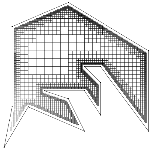
Figure 2. Whitney decomposition of a polygon. The picture was generated with software by D. E. Marshall.

8.2.

Whitney cubes and $u_{\alpha}\,.$ For a domain $G\subset{\mathbb{R}}^{n}$, $\alpha\in(0,1)$ and $z\in G$, let

$$u_{\alpha}(z)=\mathrm{cap}\,(G,\overline{B}^{n}(z,\alpha\,d(z,\partial G)))$$

and $G=\cup Q^{k}_{j}$ be a Whitney decomposition. Then $Q^{k}_{j}$ has a side length $2^{-k}$ and

$$d(Q^{k}_{j})\leq d(Q^{k}_{j},\partial G)<4d(Q^{k}_{j})=4\cdot 2^{-k}\sqrt{n}.$$

If $m^{k}_{j}$ is the midpoint of $Q^{k}_{j}$, then clearly

(8.3) $$B^{n}\left(m^{k}_{j},\frac{d(Q^{k}_{j})}{2\sqrt{n}}\right)\subset Q^{k}_{j}\subset\overline{B}^{n}\left(m^{k}_{j},\frac{d(Q^{k}_{j})}{2}\right),$$

(8.4) $$\left(1+\frac{1}{2\sqrt{n}}\right)d(Q^{k}_{j})\leq d(m^{k}_{j},\partial G)\leq\left(4+\frac{1}{2}\right)d(Q^{k}_{j}).$$

From (8.3) and (8.4), we see that

$$u_{\gamma}(m^{k}_{j})\leq\mathrm{cap}\,({\mathbb{R}}^{n}\setminus Q^{k}_{j},\partial G),\quad\gamma=\frac{d(Q^{k}_{j})/(2\sqrt{n})}{9d(Q^{k}_{j})/2}=\frac{1}{9\sqrt{n}},$$

$$u_{\eta}(m^{k}_{j})\geq\mathrm{cap}\,({\mathbb{R}}^{n}\setminus Q^{k}_{j},\partial G),\quad\eta=\frac{d(Q^{k}_{j})/2}{(1+1/(2\sqrt{n}))d(Q^{k}_{j})}=\frac{\sqrt{n}}{1+2\sqrt{n}}.$$

By Lemma 3.6, we can now observe that

$$u_{\gamma}(m^{k}_{j})\leq\mathrm{cap}\,({\mathbb{R}}^{n}\setminus Q^{k}_{j},\partial G)\leq d_{1}u_{\gamma}(m^{k}_{j}),\quad d_{1}=d_{1}(n)=\left(\frac{9\sqrt{n}}{1+2\sqrt{n}}\right)^{n-1}.$$

The next lemma follows from the the above observations.

Lemma 8.5.

For a cube $Q^{k}_{j}$ in the Whitney decomposition of the domain $G\subset{\mathbb{R}}^{n}$, let $m^{j}_{k}$ be its midpoint. Then there exists a constant $d_{1}>0$ only depending on $n$ such that

$$u_{\gamma}(m^{k}_{j})\leq\mathrm{cap}\,({\mathbb{R}}^{n}\setminus Q^{k}_{j},\partial G)\leq d_{1}u_{\gamma}(m^{k}_{j})$$

holds with $\gamma=1/(9\sqrt{n})$.

Lemma 8.6.

Let $Q^{k}_{j}$ be as in Lemma 8.5. Then there exists a constant $d_{2}>0$ only depending on $n$ such that, for all $z\in Q^{k}_{j}$,

$${u_{\gamma}(z)}/{d_{2}}\leq\mathrm{cap}\,({\mathbb{R}}^{n}\setminus Q^{k}_{j},\partial G)\leq d_{2}u_{\gamma}(z)$$

holds with $\gamma=1/(9\sqrt{n})$.

Proof.

By Theorem 3.7, $u_{\gamma}(z)$ satisfies the Harnack inequality in $G$. Therefore by [12, Lemma 6.23], there is a constant $d_{3}>0$ only depending on $n$ such that

$${u_{\gamma}(z)}/{d_{3}}\leq u_{\gamma}(m^{k}_{j})\leq d_{3}u_{\gamma}(z).$$

The proof follows now from Lemma 8.5. ∎

8.7.

Proof of Theorem 1.4. The proof follows from Lemma 8.6, Remark 7.9, and Theorem 1.5. $\square$

References

[1]L.V. Ahlfors, Ein Satz von Henri Cartan
und seine Anwendung auf die Theorie der meromorphen Funktionen
. Soc. Scient. Fenn. Comm. Phys.-Math. V. 16 (1930),1-19.
[2]L.V. Ahlfors, Conformal invariants:
Topics in Geometric Function Theory. McGraw-Hill, 1973.
[3]F. G. Avkhadiev and K.-J. Wirths,Schwarz-Pick type inequalities.
Frontiers in Mathematics. Birkhäuser Verlag, Basel, 2009.
viii+156 pp. ISBN: 978-3-7643-9999-3
[4]A.F. Beardon and D. Minda,The hyperbolic metric and geometric function theory,
Proc. International Workshop on Quasiconformal Mappings and their
Applications (IWQCMA05), (2006), 9-56.
[5]A. F. Beardon and Ch. Pommerenke,The Poincaré metric of plane domains,
J. London Math. Soc. (2) 18 (1978), no. 3, 475–483.
[6]C. J. Bishop,Harmonic measure: algorithms and
applications.
Proceedings of the International Congress of Mathematicians–
Rio de Janeiro 2018. Vol. III. Invited lectures, 1511–1537, World Sci. Publ., Hackensack, NJ, 2018.
[7]C. J. Bishop and P.W. Jones,
Hausdorff dimension and Kleinian groups.
Acta Math. 179 (1997), 1–39.
[8]P. Boyvalenkov, S. Dodunekov, and O. Musin, A survey on the kissing numbers. Serdica Math. J. 38 (2012), 507–522.
[9]V.N. Dubinin, Condenser Capacities and
Symmetrization in Geometric Function Theory, Birkhäuser, 2014.
[11]F.W. Gehring, G.J. Martin, and B.P. Palka,An introduction to the theory of higher dimensional
quasiconformal mappings, vol. 216 of Math. Surveys
and Monographs. AMS, Providence, RI, 2017.
[12]P. Hariri, R. Klén, and M. Vuorinen,Conformally invariant metrics
and quasiconformal mappings, Springer Monographs in Mathematics, Springer, Berlin, 2020.
[13]J. Heinonen,Lectures on analysis on metric spaces.
Universitext. Springer-Verlag, 2001.
[14]P. Järvi and M. Vuorinen,Uniformly perfect sets and quasiregular mappings,
J. London Math. Soc. 54 (1996), 515–529.
[15]A.
Käenmäki, J. Lehrbäck, and M. Vuorinen,
Dimensions, Whitney covers, and tubular neighborhoods.
Indiana Univ. Math. J. 62 (2013), no. 6, 1861–1889.
[16]L. Keen and N. Lakic,Hyperbolic geometry from a local viewpoint.
London Mathematical Society Student Texts, 68.
Cambridge Univ. Press, Cambridge, 2007.
[17]N. S. Landkof,Foundations of Modern Potential Theory.
Springer-Verlag, 1972.
[19]O. Martio, Capacity and measure densities. Ann. Acad. Sci.
Fenn. Ser. A I Math. 4 (1979), no. 1, 109–118.
[20]O. Martio and M. Vuorinen,Whitney cubes, p-capacity, and Minkowski content.
Exposition. Math. 5 (1987), no. 1, 17–40.
[21]P. Mattila,Geometry of sets and measures in
Euclidean spaces. Fractals and rectifiability. Cambridge Studies in
Advanced Mathematics, 44. Cambridge University Press, Cambridge, 1995.
xii+343 pp.
[23]A. Okounkov,The magic of and
Proc. ICM 2022 (to appear),
arXiv:2207.03871
[24]Ch. Pommerenke,Uniformly perfect sets and the Poincaré metric.
Arch. Math. 32 (1979), 192–199.
[25]Yu.G. Reshetnyak, The concept of capacity in the theory of functions with
generalized derivatives. (Russian) Sibirsk. Mat. Ž. 10, 1969, 1109–1138.
[26]Yu.G. Reshetnyak, Space mappings with bounded distortion.
Translated from the Russian by H. H. McFaden. Translations
of Mathematical Monographs, 73. AMS, Providence, RI, 1989. xvi+362 pp.
[27]H. Shiga and T. Sugawa,Kleinian groups and geometric
function theory. Manus. 2021
[28]E. Stein,Singular integrals and differentiability properties of functions,
Princeton Mathematical Series,
No. 30 Princeton University Press, Princeton, N.J. 1970 xiv+290 pp.
[29]T. Sugawa,Various domain constants related to uniform perfectness,
Complex Variables Theory Appl.36 (1998), 311–345.
[30]T. Sugawa, M. Vuorinen, and T. Zhang,Conformally invariant complete metrics. Math. Proc.
Cambridge Philos. Soc. 174 (2023), no 2, 273-300.
[31]J. Väisälä,Lectures on -Dimensional Quasiconformal Mappings.
Lecture Notes in Mathematics, 229. Springer-Verlag, Berlin, 1971.
[32]M. Vuorinen,Conformal geometry and quasiregular mappings.
Lecture Notes in Mathematics, 1319. Springer-Verlag, Berlin, 1988.