Thermally driven quantum refrigerator autonomously resets superconducting qubit

Abstract

The first thermal machines steered the industrial revolution, but their quantum analogs have yet to prove useful. Here, we demonstrate a useful quantum absorption refrigerator formed from superconducting circuits. We use it to reset a transmon qubit to a temperature lower than that achievable with any one available bath. The process is driven by a thermal gradient and is autonomous—requires no external control. The refrigerator exploits an engineered three-body interaction between the target qubit and two auxiliary qudits coupled to thermal environments. The environments consist of microwave waveguides populated with synthesized thermal photons. The target qubit, if initially fully excited, reaches a steady-state excited-level population of $5\times 10^{-4}\pm 5\times 10^{-4}$ (an effective temperature of 23.5 mK) in about 1.6 $\mu$s. Our results epitomize how quantum thermal machines can be leveraged for quantum information-processing tasks. They also initiate a path toward experimental studies of quantum thermodynamics with superconducting circuits coupled to propagating thermal microwave fields.

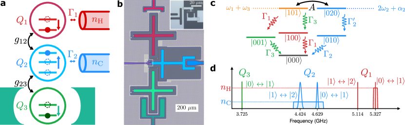
Figure 1: Absorption-refrigerator scheme and level diagram. (a) Scheme of quantum absorption refrigerator with three qudits. Qubit $Q_{1}$ couples directly to a waveguide at the rate $\Gamma_{1}$; and qudit $Q_{2}$, to another waveguide at the rate $\Gamma_{2}$. The waveguides, operating as thermal baths, host thermal photons of average numbers $n_{\rm H}$ and $n_{\rm C}$. A single excitation in $Q_{1}$ and a single excitation in $Q_{3}$ are simultaneously exchanged with a double excitation in $Q_{2}$. This exchange, occurring under a resonance condition, helps reset $Q_{3}$. (b) False-color micrograph of the device implemented with superconducting circuits. $Q_{2}$ is frequency-tunable, due to a flux current line and two parallel Josephson junctions, magnified in the inset. (c) Level diagram showing tensor products $\lvert q_{1}q_{2}q_{3}\rangle$ of the qudits’ respective energy eigenstates. $\lvert 101\rangle$ and $\lvert 020\rangle$ are resonant if $\omega_{1}+\omega_{3}=2\omega_{2}+\alpha_{2}$. At resonance, a three-body interaction couples the states at a rate $A$. (d) Distributions over the qudits’ experimentally observed transition frequencies. The Lorentzian distributions’ widths represent spectral widths. The red shaded box depicts the spectral density $n_{\rm H}$ of photons injected into the waveguide coupled to $Q_{1}$. This synthesized noise realizes the refrigerator’s hot thermal bath. Analogous statements concern the blue box, $n_{\rm C}$, $Q_{2}$, and the cold bath.

Quantum thermodynamics should be more useful. The field has yielded fundamental insights, such as extensions of the second law of thermodynamics to small, coherent, and far-from-equilibrium systems [1, 2, 3, 4, 5, 6, 7, 8, 9, 10, 11, 12, 13]. Additionally, quantum phenomena have been shown to enhance engines [14, 15, 16, 17, 18, 19], batteries [20], and refrigeration [21, 22]. These results are progressing gradually from theory to proof-of-principle experiments. However, quantum thermal technologies remain experimental curiosities, not practical everyday tools. Key challenges include control [23] and cooling quantum thermal machines to temperatures that support quantum phenomena. Both challenges require substantial energy and effort but yield small returns. For example, one would expect a single-atom engine to perform only about an electronvolt of work [24].

Autonomous quantum machines offer hope. First, they operate without external control. Second, they run on heat drawn from thermal baths, which are naturally abundant [25]. A quantum thermal machine would be useful in a context that met three criteria: (i) The machine fulfills a need. (ii) The machine can access natural different-temperature baths. (iii) Maintaining the machine’s coherence costs no extra expense.

We identify such a context: qubit reset. Consider a superconducting quantum computer starting a calculation. The computer requires qubits initialized to their ground states. If left to thermalize with its environment as thoroughly as possible, though, the qubit could achieve only an excited-state population of $\approx$0.01 to 0.03, or an effective temperature of 45 mK to 70 mK [26, 27, 28, 29]. Furthermore, such passive thermalization takes a few multiples of the qubit’s energy-relaxation time—hundreds of microseconds in state-of-the-art setups—delaying the next computation. A quantum machine cooling the qubits to their ground (minimal-entropy) states fulfills criterion (i). Moreover, superconducting qubits inhabit a dilution refrigerator formed from nested plates, whose temperatures decrease from the outermost plate to the innermost. These temperature plates can serve as heat baths, meeting criterion (ii). Finally, the machine can retain its quantum nature if mounted on the coldest plate, next to the quantum processing unit, satisfying criterion (iii). Such an autonomous machine would be a quantum absorption refrigerator.

Quantum absorption refrigerators have been widely studied theoretically [30, 31, 32, 33, 34, 35, 36, 37, 38, 39, 40, 41, 42, 40, 43, 44, 45, 46, 47, 48, 49]. Reference [50] reported a landmark proof-of-principle experiment performed with trapped ions. However, the heat baths were emulated with electric fields and lasers, rather than natural sources. Other quantum refrigerators, motivated by possible applications, have been proposed [51, 52] and tested [53, 54, 55] but are not autonomous.

We report on a quantum absorption refrigerator realized with superconducting circuits. Our quantum refrigerator cools and therefore resets a target superconducting qubit autonomously. The target qubit’s energy-relaxation time is fully determined by the temperature of a hot bath we can vary. Using this control, we can vary the energy-relaxation time by a factor of $>60$. The reset’s fidelity is competitive: The target’s excited-state population reaches as low as $5\times 10^{-4}$ (effective temperatures as low as 23.5 mK). In comparison, state-of-the-art reset protocols achieve populations of $8\times 10^{-4}$ to $2\times 10^{-3}$ (effective temperatures of 40 mK to 49 mK) [28, 29]. Our experiment demonstrates that quantum thermal machines not only can be useful, but also can be integrated with quantum information-processing units. Furthermore, such a practical autonomous quantum machine costs less control and thermodynamic work than its nonautonomous counterparts [56, 57, 58].

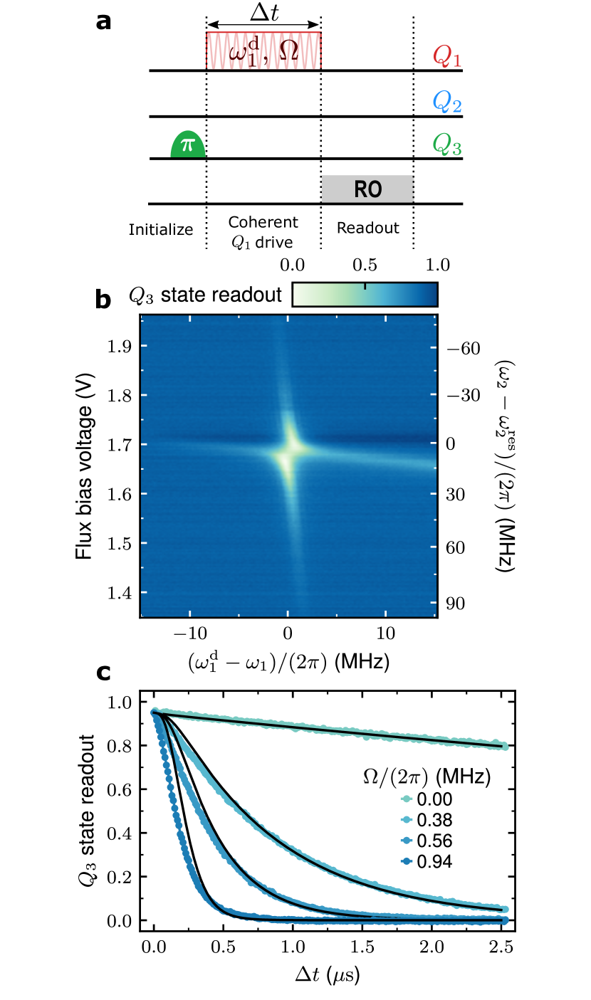
Figure 2: Three-body interaction: (a) Pulse scheme. See text for description. (b) 2D plot of $Q_{3}$’s excited-state population ($[\langle\sigma_{z}\rangle+\mathbbm{1}]/2$), as a function of (i) the flux current (left axis) modulating $Q_{2}$’s frequency and (ii) the detuning between the $Q_{1}$-drive frequency $\omega_{1}^{\rm d}/(2\pi)$ and $\omega_{1}/(2\pi)$ (bottom axis). $Q_{1}$ is driven for $\Delta t=2~{}\mu$s during the pulse scheme, after which we read out (RO) $Q_{3}$’s state via the resonator. The left axis translates directly into the right axis—the detuning of the $Q_{2}$ frequency, $\omega_{2}/(2\pi)$, from the resonant value, $\omega_{2}^{{\rm res}}/(2\pi)$. The white patch evidences an avoided crossing, where $\lvert 101\rangle$ and $\lvert 020\rangle$ become resonant (Fig. 1c). (c) $Q_{3}$’s excited-state readout, as a function of the duration $\Delta t$ of the $Q_{1}$ drive, at select drive rates $\Omega/(2\pi)$. Solid black lines are fits based on model the in Sec. II of the SI.

Our absorption refrigerator consists of three qudits ($d$-level quantum systems), as depicted in Fig. 1a. The auxiliary qudits $Q_{1}$ and $Q_{2}$ correspond to $d=2,3$, respectively. The qubit $Q_{3}$ is the target of the refrigerator’s cooling. Nearest-neighbor qudits couple together with strengths $g_{12}$ and $g_{23}$. These couplings can lead to an effective three-body interaction [59], a crucial ingredient in a quantum absorption refrigerator [30, 31, 25, 36]. We engineer the three-body interaction such that one excitation in $Q_{1}$ and one in $Q_{3}$ are simultaneously, coherently exchanged with a double excitation in $Q_{2}$. Each of $Q_{1}$ and $Q_{2}$ couples directly to a waveguide that can serve as a heat bath. Each waveguide, supporting a continuum of electromagnetic modes, can be populated with thermal photons of average number $n_{\rm H}$ or $n_{\rm C}$.

The qudits are Al-based superconducting transmons that have Al/AlO_x/Al Josephson junctions [60]. We arrange the qudits spatially in a linear configuration (Fig. 1b). The capacitances between the transmons couple them mutually. Qudit $Q_{1}$ has a transition frequency $\omega_{1}/(2\pi)=5.327$ MHz; and qudit $Q_{2}$, a variable frequency $\omega_{2}/(2\pi)$. $Q_{1}$ couples capacitively to a microwave waveguide directly, at a dissipation rate $\Gamma_{1}/(2\pi)=70$ kHz; and $Q_{2}$ couples to another waveguide at $\Gamma_{2}/(2\pi)=7.2$ MHz. The third qubit, $Q_{3}$, has a transition frequency $\omega_{3}/(2\pi)=3.725$ GHz. $Q_{3}$ couples dispersively to a coplanar waveguide resonator. Via the resonator, we read out $Q_{3}$’s state and drive $Q_{3}$ coherently. In our proof-of-concept demonstration, $Q_{3}$ stands in for a computational qubit that is being reset and that may participate in a larger processing unit. In the present design, $Q_{3}$ has a natural energy-relaxation time $T_{\rm relax}=16.8~{}\mu$s, limited largely by Purcell decay into the nearest waveguide, and a residual excited-state population $P_{0}=0.028$. In future realizations, one can increase $T_{\rm relax}$ using Purcell filters [61].

The interqudit couplings hybridize the qudit modes. The hybridization, together with the Josephson junctions’ nonlinearity, results in a three-body interaction (see SI). For this interaction to be resonant, the qudit frequencies must meet the condition $\omega_{1}+\omega_{3}=2\omega_{2}^{{\rm res}}+\alpha_{2}$. The $\omega_{2}^{{\rm res}}$ denotes the $Q_{2}$ frequency that satisfies the equality, and $\alpha_{2}$ denotes $Q_{2}$’s anharmonicity. The interaction arises from a four-wave mixing process: One excitation in $Q_{1}$ and one excitation in $Q_{3}$ are simultaneously exchanged with a double excitation in $Q_{2}$ (Fig. 1a) [59]. To control the resonance condition in situ, we make $Q_{2}$ frequency-tunable [60]. We control the frequency with a magnetic flux induced by a nearby current line. The device is mounted in a dilution refrigerator that reaches 10 mK.

To detail the resonance condition, we introduce further notation. Denote by $\lvert 0\rangle$ and $\lvert 1\rangle$ any qudit’s ground and first-excited states. Denote by $\lvert 2\rangle$ $Q_{2}$’s second excited state. We represent a three-qudit state by $\lvert q_{1}q_{2}q_{3}\rangle:=\lvert q_{1}\rangle_{1}\otimes\lvert q_{2}\rangle_{2}\otimes\lvert q_{3}\rangle_{3}$. The resonance condition implies that $\lvert 101\rangle$ and $\lvert 020\rangle$ are resonant (Fig. 1c). Two processes, operating in conjunction, reset $Q_{3}$: (i) Levels $\lvert 101\rangle$ and $\lvert 020\rangle$ coherently couple with an effective strength $A$. (ii) $Q_{2}$ dissipates into its waveguide at the rate $\Gamma_{2}$. The combined action of (i) and (ii) brings $\lvert 101\rangle$ rapidly to $\lvert 010\rangle$ (and then to $\lvert 000\rangle$), thereby resetting $Q_{3}$.

We raise the temperature of each heat bath (realized with a waveguide) as follows. We inject radiation with a thermal spectral profile over a frequency range that covers the relevant qudits’ energy-level transitions. The radiation impinging on the qudits results from admixing quantum vacuum fluctuations from a cold (10 mK) resistor and classical microwave noise synthesized at room temperature [62, 63]. We admix the ingredients using a dissipative microwave attenuator (a resistor network) functioning as a beam splitter for microwave fields. The synthesized noise has a finite bandwidth larger than $Q_{1}$’s and $Q_{2}$’s spectral widths. The noise spans a frequency range that covers $Q_{1}$’s transitions ($|0\rangle\leftrightarrow|1\rangle$) and $Q_{2}$’s transitions ($|0\rangle\leftrightarrow|1\rangle$ and $|1\rangle\leftrightarrow|2\rangle$) (Fig. 1d). This setup enables the whole system to function as a quantum thermal machine. The thermal baths induce transitions in $Q_{1}$ and $Q_{2}$, autonomously driving the reset by virtue of the three-body interaction.

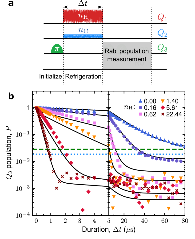
Figure 3: Autonomous refrigeration enabled by hot thermal bath. (a) 3-step pulse scheme: Initialization brings $Q_{3}$’s excited-state population close to $\lvert 1\rangle$. During refrigeration, $Q_{1}$ and $Q_{2}$ interact with synthesized thermal fields for a duration $\Delta t$. Finally, the $Q_{3}$ population, $P$, is measured via a Rabi population-measurement scheme (see SI). (b) $Q_{3}$ population as a function of the time $\Delta t$, at select values of $n_{\rm H}$, the average number of photons in the hot bath. $Q_{2}$ experiences no synthesized thermal field; due to the residual thermal field, $n_{\rm C}\approx 0.007$, we estimate. The dashed green line shows $Q_{3}$’s residual excited-state population (defined in the main text), 0.028. The dotted blue line shows the excited-state population that $Q_{3}$ would have at the cold bath’s temperature (45 mK), 0.020. The uncertainty in our $P$ measurement, 0.0005, quantifies the noise floor. As $P$ approaches 0.0005, therefore, the measured data appear to exhibit a greater dispersion. All solid lines are fits based on the model in Sec. II of the SI.

Having specified the setup, we demonstrate the three-body interaction: We verify that $Q_{3}$ can be reset via resonantly driving of Q1 if and only if $Q_{2}$ meets the resonance condition. The qudits begin in $\lvert 000\rangle$, whereupon we issue two microwave drive pulses (Fig. 2a). The first is a Gaussian $\pi$-pulse that excites $Q_{3}$ to state $|1\rangle$: $\lvert 000\rangle\rightarrow\lvert 001\rangle$. The second pulse is flat and coherently drives $Q_{1}$ (effecting $\lvert 001\rangle\leftrightarrow\lvert 101\rangle$) at the frequency $\omega_{1}^{\rm d}$ with a rate $\Omega$, for a duration $\Delta t$. Subsequently, we perform qubit-state readout on $Q_{3}$ (we measure $[\langle\sigma_{z}\rangle+\mathbbm{1}]/2$) via $Q_{3}$’s resonator. We investigate the readout’s dependences on $\omega_{1}^{\rm d}$ and on the flux current that modulates the tunable $Q_{2}$ frequency. We have fixed $\Delta t=2~{}\mu$s and $\Omega/(2\pi)=200$ kHz. The microwave drives, we observe, deplete $Q_{3}$’s excited-state population (Fig. 2a). The depletion is greatest when $\omega_{2}=\omega_{2}^{\mathrm{res}}$ and the drive is resonant ($\omega_{1}^{\rm d}=\omega_{1}$)—when the resonant coupling $A$ between $|101\rangle$ and $|020\rangle$ is strongest.

$Q_{3}$’s excited state is depleted by the cascaded processes $\lvert 001\rangle\leftrightarrow\lvert 101\rangle\leftrightarrow\lvert 020\rangle\rightarrow\lvert 010\rangle$. Away from the resonance condition, the resonant coupling $A$ decreases. Consequently, $Q_{3}$’s excited-state population drops less as the $\lvert 101\rangle$–$\lvert 020\rangle$ detuning grows. Furthermore, we study the effect of increasing $\Omega$ (Fig. 2c). When $\Omega=0$ MHz, $Q_{3}$ decays to its ground state (resets) at its natural energy-relaxation time, $T_{\rm relax}$. As $\Omega$ increases, the reset happens increasingly quickly. According to our model’s fit to these results, the 3-body interaction strength is $A/(2\pi)=3.2$ MHz.

Having demonstrated the three-body interaction, we operate the three-qubit system as a quantum thermal machine. To measure the system’s performance, we implement a three-step pulse sequence (Fig. 3a): (i) Excite $Q_{3}$ to near $|1\rangle$ (to an excited-state population of 0.95). (ii) Fill the waveguides with the thermal photons, as described above, for a variable time interval $\Delta t$. (iii) Measure $Q_{3}$’s excited-state population, using a Rabi population-measurement scheme [26, 27] (see Sec. III of the Supplementary Information [SI] for details). This scheme allows for a more accurate population measurement than does standard qubit-state readout.

We raise the hot bath’s effective temperature and investigate how $Q_{3}$’s excited-state population, $P$, responds. To do so, we elevate the average number $n_{\rm H}$ of thermal photons in the hot bath, by increasing the spectral power of the synthesized noise in $Q_{1}$’s waveguide. We perform this study in the absence of synthesized noise in the cold bath (coupled to $Q_{2}$). In independent measurements, we determine the cold bath’s average number of thermal photons: $n_{\rm C}=0.007$, associated with a temperature $T_{\rm C}=45$ mK. The greater the $n_{\rm H}$, the more quickly $P$ decays as we increase $\Delta t$ (Fig. 3b). At the low value $n_{\rm H}=0.16$, $P$ drops below the residual excited-state population $P_{0}$ (green dashed line in Fig. 3b), which $Q_{3}$ would achieve if left alone for a long time. The residual population corresponds to an effective temperature of $T_{\rm T}=50$ mK. If thermalized at the cold bath’s temperature (45 mK), $Q_{3}$ would have an excited-state population $P_{0}=0.020$ (blue dotted line). Notably, if the hot bath is excited, $Q_{3}$ reaches a steady-state population $P_{{\rm SS}}$ an order of magnitude lower than $P_{0}$ and $P_{\rm C}$. Our refrigeration scheme clearly outperforms passive thermalization with either $Q_{3}$’s intrinsic bath or the coldest bath available.

At $n_{\rm H}=21.424$ ($T_{\rm H}=5.6$ K), the refrigeration reduces $Q_{3}$’s effective energy-relaxation time, $T_{\rm relax}$, from $16.8~{}\mu$s to $250$ ns, a reduction by a factor of over 60. $Q_{3}$’s population declines to $2\times 10^{-3}$ over $1.6~{}\mu$s, before asymptotically approaching a steady state. We define $Q_{3}$’s steady-state population as $P_{{\rm SS}}\coloneqq P(\Delta t=100~{}\mu\mathrm{s})$. $P_{{\rm SS}}$ reaches a minimum of $5\times 10^{-4}\pm 5\times 10^{-4}$, equivalent to a temperature of $23.5$ mK.

A refrigerator’s thermodynamic figure of merit is its coefficient of performance (COP) [36]. The COP equals the heat current expelled by the target, divided by the heat current drawn by $Q_{1}$ from the hot bath. We calculate the steady-state COP numerically from the theoretical model in Sec. II of the SI. The steady-state COP is 0.7 when $T_{\rm H}=5.6$ K and $T_{\rm T}=23.5$ mK. The Carnot bound on our COP is $\frac{T_{\rm T}(T_{\rm H}-T_{\rm C})}{T_{\rm H}(T_{\rm C}-T_{\rm T})}=1.1>0.7$. For comparison, a common autonomous air conditioner has a COP of $\approx 0.7$ [64].

Another important performance metric is the time required to reset $Q_{3}$. We define the reset time as the time required for $P$ to reach $0.01$ (corresponding to $38.5$ mK). The reset time reaches as low as 970 ns before rising slowly with $n_{\rm H}$ (Fig. 4a). Now, we study $P_{{\rm SS}}$ as a function of $n_{\rm H}$ or $n_{\rm C}$, while keeping the other quantity fixed. $P_{{\rm SS}}$ decreases rapidly as $n_{\rm H}$ increases (Fig. 4b). $P_{{\rm SS}}$ reaches its lowest value when $n_{\rm C}$ minimizes at $0.007$, such that $Q_{2}$ is not excited. On the other hand, raising the cold bath’s temperature impedes the reset. Increasing $n_{\rm C}$ to 0.07—exciting $Q_{2}$ more—leads $P_{{\rm SS}}$ to saturate at a higher value. Finally, consider fixing $n_{\rm H}$ and varying $n_{\rm C}$. $P_{{\rm SS}}$ increases rapidly, then saturates near 0.36. This saturation occurs largely independently of $n_{\rm H}$. The greater the $n_{\rm H}$, though, the greater the initial $P_{{\rm SS}}$.

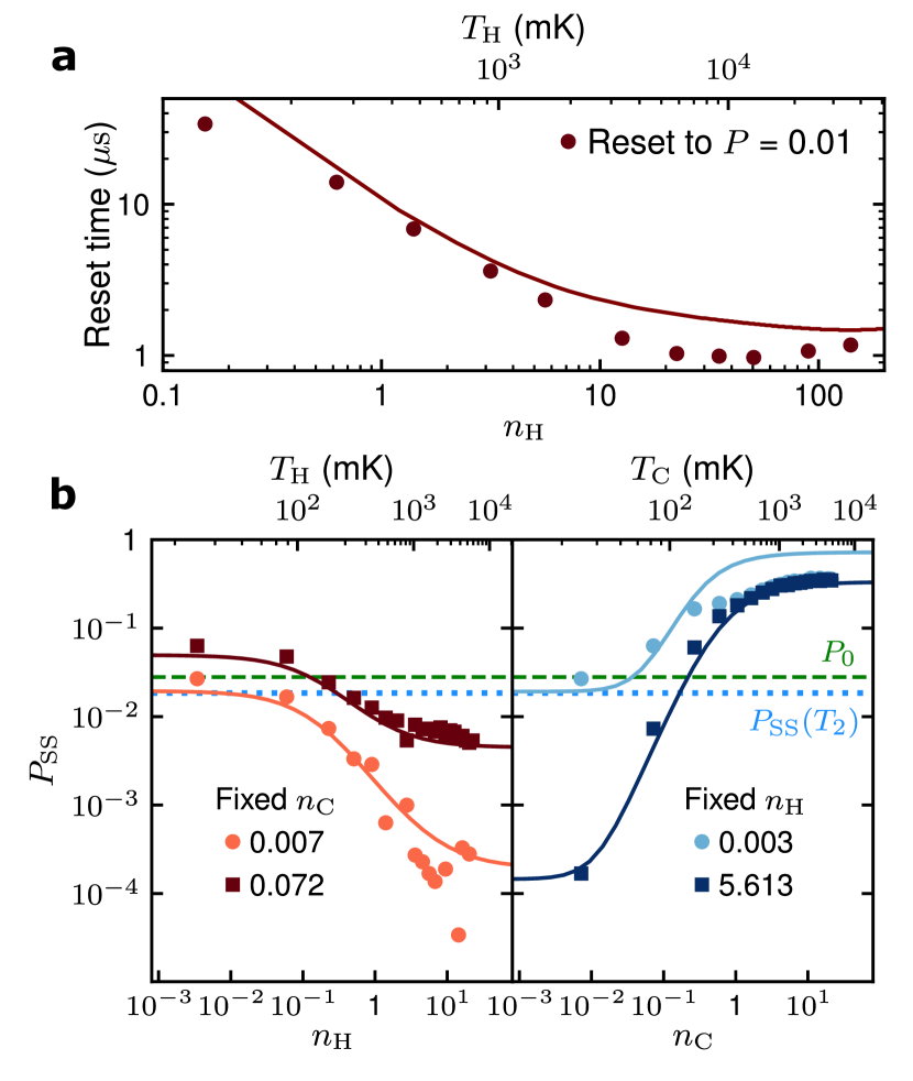
Figure 4: Metrics of the quantum absorption refrigerator. (a) Reset time (time required for $Q_{3}$’s excited-state population to reach 0.01), as a function of the hot bath’s average photon number, $n_{\rm H}$. (b) (Left) After a 100 $\mu$s reset protocol, $Q_{3}$’s excited state reaches a steady-state population $P_{{\rm SS}}$. The $x$-axis shows $n_{\rm H}$, translated into a temperature $T_{\rm H}$ along the top axis. Colors distinguish values of the cold bath’s average photon number, $n_{\rm C}$. (Right) $P_{{\rm SS}}$ as a function of $n_{\rm C}$ (translated into a temperature $T_{\rm C}$ on the top axis), at two $n_{\rm H}$ values. The dashed green line shows $Q_{3}$’s residual excited-state population, 0.028. The dotted blue line shows the excited-state population that $Q_{3}$ would have at the cold bath’s temperature (45 mK), 0.020. All solid lines are theoretical predictions calculated from the model in Sec. II of the SI.

In summary, we have demonstrated the first quantum thermal machine being deployed to accomplish a useful task. The task—reset of a superconducting qubit—is crucial to quantum information processing. The machine—a quantum absorption refrigerator formed from superconducting circuits—cools and resets the target qubit to an excited-state population lower than that achieved with state-of-the-art active reset protocols, without requiring external control. Nevertheless, the refrigeration can be turned off during the target qubit’s computation cycle: One can either change the hot bath’s temperature or detune a qudit out of resonance, using on-chip magnetic flux.

A salient feature of our quantum thermal machine is its use of waveguides as physical heat baths. In contrast, other experiments have emulated heat baths [57, 50]. Our heat baths consist of thermal photons synthesized from quantum vacuum fluctuations and artificial microwave noise within a finite bandwidth. Our approach allows control over the baths’ temperatures, the ability to tailor spectral properties of the heat baths, and the selection of the energy transitions to be heated. Thus, this method can facilitate a rigorous study of quantum thermal machines. However, our setup can be straightforwardly modified to exploit natural thermal baths, such as different-temperature plates of a dilution refrigerator. For example, superconducting coaxial cables, together with infrared-blocking filters [65], can expose the qudits to thermal radiation emitted by hot resistors anchored to the dilution refrigerator’s plates [66]. This strategy refrains from adding any significant heat load to the base temperature plate. Nor does the strategy compromise the quantum information-processing unit’s performance.

Our quantum refrigerator initiates a path toward experimental studies of quantum thermodynamics with superconducting circuits coupled to propagating thermal microwave fields. Superconducting circuits may also offer an avenue toward scaling quantum thermal machines similarly to quantum-information processors. Our experiment may inspire further development of useful, real-world applications of quantum thermodynamics to quantum information processing [67, 68, 69], thermometry [70, 63, 66], algorithmic cooling [53, 71], timekeeping [72], and entanglement generation [73]. This work marks a significant step in quantum thermodynamics toward practicality, in the spirit of how classical thermodynamics aided the industrial revolution.

Supplementary information

A Full experimental setup and parameters

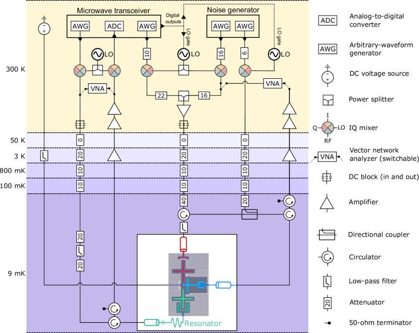
Figure S1: Complete experimental set-up. See text for description. The in-phase-quadrature (IQ) mixers’ ports I and Q are both used to connect to the microwave transceiver. However, only port I is shown to be wired; port Q is omitted for clarity. Digital outputs from the microwave transceiver are used to gate the local oscillators (LO) to produce pulses of thermal microwave modes.

Figure S1 shows a schematic of the experimental set-up used to study our quantum absorption refrigerator (QAR). The QAR is packaged in a copper enclosure and mounted on the mixing-chamber stage of a dilution refrigerator that reaches 9 mK. The QAR is packaged in multiple layers: two nested copper enclosures shield the QAR from electromagnetic waves. A $\mu$-metal enclosure protects the QAR from low-frequency magnetic fields. Microwave fields (both coherent and thermal) are routed to the QAR through highly attenuated input coaxial lines. The outgoing fields are routed through the output lines and are boosted by a cryogenic high electron-mobility transistor (HEMT) amplifier (provided by Low Noise Factory) at 3 K and by room-temperature amplifiers. Microwave circulators separate the input and output signals. The resonator, dispersively coupled to qubit $Q_{3}$, is probed by a microwave feedline in reflection mode. We probe and drive $Q_{1}$ and $Q_{2}$, via the waveguide coupled to each, using two attenuated coaxial lines. Taking advantage of the non-overlapping frequencies of the relevant transitions, the outgoing fields from the hot and the cold waveguide are combined with the aid of a directional coupler and forwarded to the same output line.

We use a microwave transceiver (Vivace from Intermodulation Products, Sweden), with in-phase-quadrature (IQ) mixers and local oscillators (LO), for driving the qudits and for readout measurements of $Q_{3}$. The physical connections can be switched to a vector network analyzer (VNA). The VNA is used for continuous-wave spectroscopy that allows for basic characterization, e.g., of a qudit’s frequency and anharmonicity.

The waveguide coupled to $Q_{1}$ is populated with synthesized thermal microwave modes limited to a 50 MHz bandwidth centered at the qubit’s frequency. An analogous statement concerns the waveguide coupled to $Q_{2}$. To populate the waveguides, we first continuously generate voltage noise with a white (flat) spectral density, using an arbitrary-waveform generator (AWG) limited to a 50 MHz bandwidth centered at a frequency of 100 MHz. The equipment used is a Keysight 3202A, which is limited to a 500 MHz bandwidth. Next, the generated noise is up-converted with IQ mixers and microwave tones ($\approx$ 4 GHz to 6 GHz) generated by an LO. Finally, the resulting continuous thermal radiation is chopped into pulses synchronized with $Q_{3}$-state readouts (see Fig. 3 in the main text). This process was performed via modulation (gating) of the LO outputs (Anapico APMS20G-4-ULN), with help from the transceiver’s digital logic outputs, over time intervals of 10 ns and longer. To characterize the qudits (e.g., to determine their frequencies), we can switch the input/output lines to VNA. Furthermore, to observe the three-body interactions with coherent drives (see Fig. 2 in the main text), we can switch qubit $Q_{1}$’s input line to the transceiver’s AWG. (Certain equipment, instruments, software, or materials are identified in this paper in order to specify the experimental procedure adequately. Such identification is not intended to imply recommendation or endorsement of any product or service by NIST, nor is it intended to imply that the materials or equipment identified are necessarily the best available for the purpose.)

Table S1 shows the QAR’s experimentally inferred parameters.

Parameter	Symbol	Value
$Q_{1}$ mode frequency	$\omega_{1}/(2\pi)$	5.327 GHz
$Q_{2}$ mode-tunable frequency range	$\omega_{2}/(2\pi)$	4.2 GHz to 4.9 GHz
$Q_{2}$ resonant frequency	$\omega_{2}^{\rm res}/(2\pi)$	4.629 GHz
$Q_{3}$ mode frequency	$\omega_{3}/(2\pi)$	3.725 GHz
$Q_{1}$ anharmonicity	$\alpha_{1}/(2\pi)$	-213.4 MHz
$Q_{2}$ anharmonicity	$\alpha_{2}/(2\pi)$	-205.1 MHz
$Q_{3}$ anharmonicity	$\alpha_{3}/(2\pi)$	-237.8 MHz
$Q_{1}$ radiative-emission rate	$\Gamma_{1}/(2\pi)$	70 kHz
$Q_{2}$ radiative-emission rate	$\Gamma_{2}/(2\pi)$	7.2 MHz
$Q_{3}$ energy-relaxation time	$T_{\rm relax}$	16.8 $\mu$s
Three-body-coupling rate	$A/(2\pi)$	3.2 MHz

Table S1: Experimentally measured parameters’ values.

B Theoretical model

The Hamiltonian of our QAR’s three-qudit system can be written as

$$H=\sum_{i=1}^{3}\left(\tilde{\omega}_{i}\hat{\tilde{a}}^{\dagger}_{i}\hat{\tilde{a}}_{i}+\alpha_{i}\hat{\tilde{a}}^{\dagger}_{i}\hat{\tilde{a}}^{\dagger}_{i}\hat{\tilde{a}}_{i}\hat{\tilde{a}}_{i}/2\right)+g_{12}\left(\hat{\tilde{a}}^{\dagger}_{1}\hat{\tilde{a}}_{2}+\hat{\tilde{a}}_{1}\hat{\tilde{a}}^{\dagger}_{2}\right)+g_{23}\left(\hat{\tilde{a}}^{\dagger}_{2}\hat{\tilde{a}}_{3}+\hat{\tilde{a}}_{2}\hat{\tilde{a}}^{\dagger}_{3}\right).$$ (S1)

$\hat{\tilde{a}}_{i}$ and $\hat{\tilde{a}}^{\dagger}_{i}$ denote qudit $Q_{i}$’s annihilation and creation operators. $\tilde{\omega}_{i}$ and $\alpha_{i}$ denote qudit $Q_{i}$’s bare mode frequency and anharmonicity. $g_{12}$ ($g_{23}$) denotes the rate of the coupling between qudits $Q_{1}$ and $Q_{2}$ (qudits $Q_{2}$ and $Q_{3}$).

We engineer an effective three-body interaction by meeting the resonance condition $\omega_{1}+\omega_{3}=2\omega_{2}+\alpha_{2}$ and using Josephson junctions that facilitate the four-wave mixing [59]. The three-body interaction interchanges the three-qudit states $\lvert 101\rangle$ and $\lvert 020\rangle$ (see the notation and Fig. 1c in the main text).

We now introduce an approximation to $H$. Denote by $A$ the rate at which $\lvert 101\rangle$ and $\lvert 020\rangle$ couple coherently. $H$ is well-approximated by the effective Hamiltonian

$$H_{\rm eff}=\sum_{i=1}^{3}\omega_{i}\hat{a}^{\dagger}_{i}\hat{a}_{i}+\sum_{i,j=1}^{3}\frac{\alpha_{ij}}{2}\hat{a}^{\dagger}_{i}\hat{a}_{i}\hat{a}^{\dagger}_{j}\hat{a}_{j}+A\left(\lvert 101\rangle\langle 020|+\lvert 020\rangle\langle 101|\right).$$ (S2)

The simplification follows from black-box quantization [74] and second-order time-independent perturbation theory [59]. $H_{\rm eff}$ depends on dressed modes associated with annihilation and creation operators $\hat{a}_{i}$ and $\hat{a}^{\dagger}_{i}$, dressed-mode frequencies $\omega_{i}$, and self and cross-Kerr coupling rates $\alpha_{ij}$.

Let us introduce into the model a drive as shown in Fig. 2 of the main text. This coherent drive is applied to $Q_{1}$ at the drive frequency $\omega_{\rm d}$ and the rate $\Omega$. Upon adding a drive term to $H_{\rm eff}$, we apply the rotating-wave approximation. We obtain the full Hamiltonian

$$H_{\rm D1}=\sum_{i=1}^{3}\delta_{i}\hat{a}^{\dagger}_{i}\hat{a}_{i}+\sum_{i,j=1}^{3}\frac{\alpha_{ij}}{2}\hat{a}^{\dagger}_{i}\hat{a}_{i}\hat{a}^{\dagger}_{j}\hat{a}_{j}+A\left(\lvert 101\rangle\langle 020|+\lvert 020\rangle\langle 101|\right)+\frac{\Omega}{2}\left(\hat{\tilde{a}}_{1}+\hat{\tilde{a}}^{\dagger}_{1}\right).$$ (S3)

The effective frequency $\delta_{i}=\omega_{d}-\omega_{i}$.

To model the measurements of Fig. 2, we solve a Lindblad quantum master equation:

$$\frac{\partial\rho}{\partial t} =-\frac{i}{\hbar}[H_{D1},\rho]+\sum_{i=1}^{3}\Gamma_{i}\mathcal{D}[\hat{\tilde{a}}_{i},\rho].$$ (S4)

We model the waveguides as zero-temperature baths (with average occupation numbers of 0). The qudits can interact with such baths just through spontaneous emission [75]. We have suppressed the time dependence of $\rho$ in our notation. $\Gamma_{i=1,2}$ denotes the rate at which qudit $Q_{i}$ couples to its waveguide. $\Gamma_{3}$, $Q_{3}$’s natural energy-relaxation rate, is related to the qubit’s energy-relaxation time $T_{\rm relax}$ through $\Gamma_{3}=1/T_{\rm relax}$. The dissipator superoperator $\mathcal{D}$ is defined through

$$\mathcal{D}[A,B]=ABA^{\dagger}-\frac{1}{2}\left(A^{\dagger}AB+BA^{\dagger}A\right),$$ (S5)

for operators $A$ and $B$.

To model the QAR interacting with two heat baths, we limit our analysis to a subspace of the full Hilbert space. This subspace is spanned by the basis $\mathcal{B}=\{\lvert 000\rangle,\lvert 100\rangle,\lvert 010\rangle,\lvert 001\rangle,\lvert 020\rangle,\lvert 101\rangle\}$. The population of $\lvert i\rangle\in\mathcal{B}$ is $p_{i}\coloneqq\rho_{ii}\coloneqq\langle i\rvert\rho\lvert i\rangle$. We formulate a rate equation for these populations. To capture the coherent exchanges between $\lvert 101\rangle$ and $\lvert 020\rangle$, we also include an off-diagonal element $\rho_{\rm coh}=\langle 101\rvert\rho\lvert 020\rangle$ in the model. Combining these ingredients, we introduce the rate equation for the populations:

$$\frac{d}{dt}\begin{pmatrix}p_{\lvert 000\rangle}(t)\\ p_{\lvert 100\rangle}(t)\\ p_{\lvert 010\rangle}(t)\\ p_{\lvert 001\rangle}(t)\\ p_{\lvert 020\rangle}(t)\\ p_{\lvert 101\rangle}(t)\\ \rho_{\rm coh}(t)\end{pmatrix}=R_{\rm P}\begin{pmatrix}p_{\lvert 000\rangle}(t)\\ p_{\lvert 100\rangle}(t)\\ p_{\lvert 010\rangle}(t)\\ p_{\lvert 001\rangle}(t)\\ p_{\lvert 020\rangle}(t)\\ p_{\lvert 101\rangle}(t)\\ \rho_{\rm coh}(t)\end{pmatrix}.$$ (S6)

The rate matrix $R_{\rm P}$ is defined as

$$R_{\rm P}\coloneqq\left(\begin{array}[]{ccccccc}-\Gamma_{1\uparrow}+\Gamma_{2\uparrow}+\Gamma_{3\uparrow}&\Gamma_{1\downarrow}&\Gamma_{2\downarrow}&\Gamma_{3\downarrow}&0&0&0\\ \Gamma_{1\uparrow}&-(\Gamma_{1\downarrow}+\Gamma_{3\uparrow})&0&0&0&\Gamma_{3\downarrow}&0\\ \Gamma_{2\uparrow}&0&-(\Gamma_{2\downarrow}+2\Gamma_{2\uparrow})&0&2\Gamma_{2\downarrow}&0&0\\ \Gamma_{3\uparrow}&0&0&-(\Gamma_{3\downarrow}+\Gamma_{1\uparrow})&0&\Gamma_{1\downarrow}&0\\ 0&0&2\Gamma_{2\uparrow}&0&-2\Gamma_{2\downarrow}&0&2A\\ 0&\Gamma_{3\uparrow}&0&\Gamma_{1\uparrow}&0&-(\Gamma_{1\downarrow}+\Gamma_{3\downarrow})&-2A\\ 0&0&0&0&-A&A&\Gamma_{\rm C}\end{array}\right)$$ (S7)

We define the $\Gamma$’s as follows. Denote by $n_{i}$ the average number of synthesized thermal photons in the waveguide coupled to qudit $Q_{i}$; by $n_{i,{\rm res}}$, the average number of native thermal (residual) photons already present in waveguide $i=1,2$; and by $n_{\rm{3,res}}$, the effective average number of thermal photons in qudit $Q_{3}$’s environment. In terms of these quantities, we define lowering rates $\Gamma_{i\downarrow}=\Gamma_{i}(n_{i}+n_{i,{\rm res}}+1)$ and raising rates $\Gamma_{i\uparrow}=\Gamma_{i}(n_{i}+n_{i,{\rm res}})$ for the qudits $i=\{1,2\}$, as well as $\Gamma_{3\downarrow}=\Gamma_{3}(n_{i,{\rm res}}+1)$ and $\Gamma_{3\uparrow}=\Gamma_{3}n_{i,{\rm res}}$. For brevity, Eq. (S7) also contains $\Gamma_{\rm C}=(-2\Gamma_{2\downarrow}+2\Gamma_{2\uparrow}+\Gamma_{1\downarrow}+\Gamma_{1\uparrow}+\Gamma_{3\downarrow}+\Gamma_{3\uparrow})/4$.

To model the data in Figs. 3b and 4b, we solve Eq. (S6) with the initial condition

$$\mathbf{(}p_{\lvert 000\rangle}(0),p_{\lvert 100\rangle}(0),p_{\lvert 010\rangle}(0),p_{\lvert 001\rangle}(0),p_{\lvert 020\rangle}(0),p_{\lvert 101\rangle}(0),\rho_{\rm coh}(0)\mathbf{)}=(0,0,0,1,0,0,0).$$

This vector represents the initial state $\lvert 001\rangle$.

Having introduced our dynamical model, we review the coefficient of performance (COP), following Ref. [36]. Denote by $\mathcal{Q}_{3}$ the current of heat drawn from the target system. Denote by $\mathcal{Q}_{1}$ the current of heat drawn by qubit 1 from the hot bath. An absorption refrigerator’s COP equals the ratio of one to the other:

$$\text{COP}\coloneqq\dot{\mathcal{Q}}_{3}/\dot{\mathcal{Q}}_{1}\,.$$ (S8)

We calculate the COP at the refrigerator’s steady state. The steady-state heat current drawn from bath $i\in\{1,2,3\}$ is

$$\dot{Q}_{i}=\operatorname{Tr}\mathbf{(}H\mathcal{L}_{i}\rho(\infty)\mathbf{)}.$$ (S9)

The Lindbladian therein acts as $\mathcal{L}_{i}\rho=\Gamma_{i}\left\{\left(n_{i}+n_{i,{\rm res}}+1\right)\mathcal{D}[{\tilde{a}}_{i},\rho]+(n_{i}+n_{i,{\rm res}})\mathcal{D}[{\tilde{a}}_{i}^{\dagger},\rho]\right\}$.

C Rabi population-measurement scheme

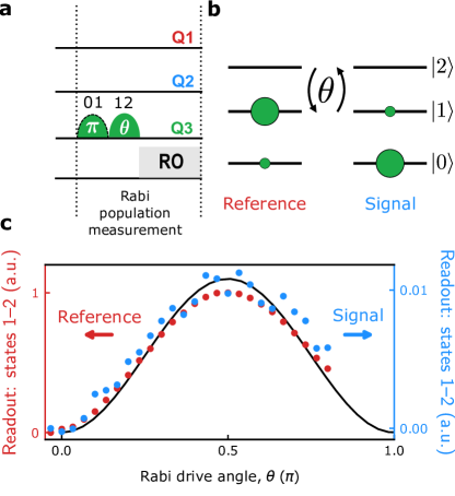
Figure S2: Rabi measurement of the population in qubit $Q_{3}$’s $\lvert 1\rangle$ level. (a) Pulse sequence for the scheme. The notation 0–1 (1–2) indicates that the pulse drives the transition $|0\rangle\leftrightarrow|1\rangle$ ($|1\rangle\leftrightarrow|2\rangle$). $\theta$ denotes the pulse drive’s Rabi angle. The pulse with the dashed outline is present in the reference measurement and absent from the signal measurement. The readout (RO) is performed in the subspace ${\rm span}\{|1\rangle,|2\rangle\}$. (b) Representation of the relative distribution of populations across $|0\rangle$, $|1\rangle$, and $|2\rangle$. (c) Rabi oscillations. The Rabi oscillation resulting from the 1–2 pulse provides a reference trace (red). The Rabi oscillation produced without the 1–2 pulse provides the signal—the actual population trace (blue).

Figure S2 shows the pulse sequence for measuring $Q_{3}$’s level-$\lvert 1\rangle$ population more accurately than standard qubit readout allows [26, 27]. This Rabi scheme involves the $Q_{3}$ energy levels $|0\rangle$, $|1\rangle$, and $|2\rangle$. (We measure the qubit-state readout in the subspace ${\rm span}\{|1\rangle,|2\rangle\}$.) The scheme involves also two different Rabi oscillations. We drive Rabi oscillations between $|1\rangle$ and $|2\rangle$ in each of two cases: with and without a prior $\pi$ pulse in the subspace ${\rm span}\{|0\rangle,|1\rangle\}$. The prior pulse interchanges the populations of $|0\rangle$ and $|1\rangle$ [see the 0–1 pulse with the dashed outline in Fig. S2(a)]. We denote these Rabi oscillations’ amplitudes by $r$ and $s$, respectively. The population of $Q_{3}$’s $|1\rangle$ state is $s/(r+s)$. This method works if $|2\rangle$ is empty and so can serve as a reference for zero population.

D Refrigeration’s dependence on cold-bath temperature

Figure S3: Refrigeration’s dependence on cold-bath temperature. (a) Pulse scheme. (b) Population of qubit $Q_{3}$’s $\lvert 1\rangle$ level, as a function of the time duration $\Delta t$ of the thermal-microwave-mode pulses, at select values of the average number $n_{\rm C}$ of thermal photons in the cold bath. The average number $n_{\rm H}$ of thermal photons in the hot bath is fixed at the high value 35.

Figure S3 shows the population of $Q_{3}$’s $\lvert 1\rangle$ state, $P$. We depict $P$ as a function of the duration $\Delta t$ for which the thermal microwave modes are applied. We present these data at several values of the average number $n_{\rm C}$ of photons in the cold bath. The average number $n_{\rm H}$ of hot-bath thermal photons is a high value, 35.

Increasing $n_{\rm C}$ populates $Q_{2}$’s excited states incoherently, rendering the qutrit’s state mixed [63]. The mixing hinders the three-body process $\lvert 101\rangle\rightarrow\lvert 020\rangle$. The refrigeration is impeded, and so the steady-state $P$ increases.

E Refrigeration of $Q_{3}$ initiated in its natural steady state

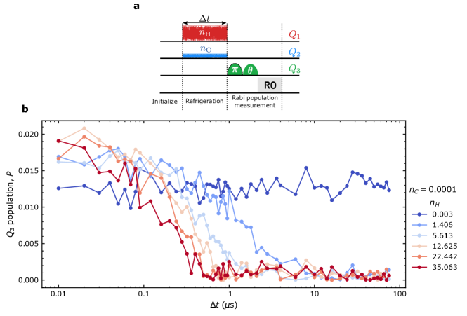
Figure S4: Refrigeration of target qubit initialized with a residual $\lvert 1\rangle$ population of 0.020. (a) Pulse scheme. The qubit is not initialized entirely in the excited state. (b) $Q_{3}$’s excited-state population, $P$, as a function of the time duration $\Delta t$ of the thermal-microwave-mode pulses, for select values of the average number $n_{\rm H}$ of thermal photons in the hot bath.

In this study, we begin with $Q_{3}$ in the steady state that results from $Q_{3}$’s equilibrating as much as possible with its environment (the state may, in fact, be far from equilibrium). According to our measurements, $Q_{3}$’s $\lvert 1\rangle$ level has a population $P$ of $0.028$ in this state. We allow our refrigerator to run for a duration $\Delta t$, then perform Rabi population measurement of $\lvert 1\rangle$. (See the pulse scheme in Fig. S4a.) $P$ is plotted as a function of $\Delta t$ in Fig. S4. Here, $P$ begins at a much less value than in the main text’s Fig. 3b. Therefore, $P$ reaches its long-time value, here, by an earlier time $\approx 500$ ns.