Localization under consistent assumptions over dynamics

Abstract

Accurate maps are a prerequisite for virtually all autonomous vehicle tasks. Most state-of-the-art maps assume a static world, and therefore dynamic objects are filtered out of the measurements. However, this division ignores movable but non-moving, i.e., semi-static, objects, which are usually recorded in the map and treated as static objects, violating the static world assumption, causing error in the localization. In this paper, we present a method for modeling moving and movable objects for matching the map and the measurements consistently. This reduces the error resulting from inconsistent categorization and treatment of non-static measurements. A semantic segmentation network is used to categorize the measurements into static and semi-static classes, and a background subtraction-based filtering method is used to remove dynamic measurements. Experimental comparison against a state-of-the-art baseline solution using real-world data from Oxford Radar RobotCar data set shows that consistent assumptions over dynamics increase localization accuracy.

I Introduction

Mapping is a central functionality of mobile robot systems, since an accurate representation of the environment, i.e., a map, is a prerequisite for many crucial functionalities, such as localization and path planning.

The majority of existing mapping methods assume that the mapped environment does not change until the map is used for localization. This is usually referred to as the static world assumption. The assumption is made for simplicity even if it does not fully hold. Violations of the assumption, however, may result in errors in the localization.

For example, the map might contain parked cars which would be considered equally reliable landmarks compared to non-movable, i.e., static, objects such as buildings. If during localization another car was observed in a different pose than the car in the map that has since left, the potential incorrect match may cause localization error. This phenomenon is illustrated in Figure 1.

To address this problem, many methods for removing moving, i.e., dynamic, objects from the measurements have been proposed [1, 2, 3, 4, 5, 6], and it continues to be the most common approach in the state-of-the-art localization and mapping methods. This dichotomy between moving and non-moving objects ignores objects that are movable, while not currently moving. In this work we call such objects semi-static objects, and assume that the environment consists of objects from these three dynamic classes: static, semi-static and dynamic.

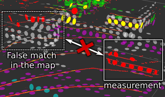
Figure 1: Semi-static objects treated as static violate the static world assumption and cause mismatches between the map and the measurements. In this example, the map contains a parked car (left rectangle) which has since moved away. When the autonomous vehicle comes back, an observed parked car (right rectangle) is offset from the one on the map. This offset causes matching errors especially when the difference in poses is small, or other features in the direction of the error are lacking or sparse.

With the increased performance of semantic segmentation networks, it is possible to detect semi-static objects directly from laser measurements. However, proper representation of the dynamic classes in maps is still rare, and semi-static objects are usually treated as static, violating the static world assumption.

In this work we show a better way: by distinguishing between the properties of movability and motion, we can properly model the dynamic, semi-static, and static parts of the environment. With the consistent application of this distinction, we are in compliance with not only the static world assumption, but consistent in all our assumptions over dynamics. By using real-world data from real traffic scenarios gathered over nine days, we show that localization under consistent assumptions over dynamics increases localization accuracy.

Using semantic segmentation of laser point clouds and background subtraction and clustering-based dynamic object filtering, we can partition the measurements into dynamic classes. To be consistent in the assumptions over dynamics, using these filters we create an Normal Distributions Occupancy Map (NDT-OM) [5] containing only static measurements. For comparison, we use the state-of-the-art baseline NDT-OM which does not discriminate between semi-static and static measurements and therefore violates the static world assumption.

Similarly we use the aforementioned filters to demonstrate four localization methods based on Normal Distributions Transform Monte-Carlo Localization (NDT-MCL) [7], each using measurements of different dynamic classes in the localization. Subsequently, we show the localization accuracy is best when we match the measurements with the maps under consistent assumptions over dynamics.

The main contributions of this paper are:

1. We propose a localization method using semantic segmentation and dynamic filtering to remove non-static measurements from the input measurements of the localization.

2. We propose a mapping method using semantic segmentation to remove non-static measurements to produce a map compliant with the static world assumption.

3. We show with an empirical study consisting of 112 localization experiments that the localization accuracy of the baseline NDT-MCL can be improved using the proposed mapping method to create a map consisting of only static measurements as well as the proposed localization method.

II Related work

II-A Filtering dynamic objects

The most commonly used type of map in mobile robotics is the occupancy map [8]. Occupancy maps incorporate the static world assumption, as they do not model the dynamic properties of the contents of the cells.

While dynamic objects appear on the maps, they are removed after the occupied space has been observed empty by the virtue of the free space modeling by the inverse sensor model. While this approach is widely used, it has several problems. For the dynamic objects to be removed, the space must be perceived empty, so at the end of the mapping sequence, or at the point of transition to a different area, there is a high probability that dynamic objects will remain in the map. Additionally, the map does not represent the dynamic properties of the measurements in the map, so the sensor model cannot be adjusted to update the probabilities depending on the dynamic properties of the measurement and the affected grid cells.

To alleviate these problems, methods to filter dynamic objects from the measurements directly have been proposed [1, 2, 3, 4].

Even if dynamic objects are filtered from the measurements, unlike this work, none of these approaches distinguish between static and semi-static objects, and subsequently leave the semi-static objects in the map.

II-B Representation of semi-static objects

To address the issue of semi-static objects being treated as static, several methods have been proposed. Semi-static objects have been represented as separate temporary maps [9] with a given static map. The dynamics are not modeled explicitly, rather the proposed method stores multiple maps from different times as static snapshots of the different states of the environment, and selects the map which explains the current measurement the best. While this is not done to create a consistent representation of the environment, but rather to facilitate localization, this idea extends similar methods that jointly localize the robot and estimate the state of the environment, demonstrated multiple times with a door [10, 11].

A step forward in representing the dynamic nature of the environment is to model it as an Hidden Markov Model (HMM) [12, 13]. While an HMM models explicitly the belief of occupancy and the transition probabilities of the environment, which can be used to improve the localization accuracy, but unlike this work, there is no distinction between dynamic or static cells.

Furthermore, the static world assumption is ingrained into the Markov assumptions of independence of odometry and observations. These assumptions have been relaxed by partitioning the localization experiment into episodes that are internally Markovian, but as a whole are not [14]. In this work, we aim instead to maintain a consistent environment representation.

While static objects are considered not to be movable, semi-static objects are likely to move during the lifetime of a map. Therefore the probability of any object to remain stationary reduces over time. This degree of staticness can be modeled explicitly as decaying probability of the persistence of a feature [15]. Features are more naturally linked to object instances that can be ascribed with a notion of staticness, whereas we model the dynamic properties of the entire spatial environment directly.

Moreover, the dominant testing environment in modeling semi-static objects so far has been the parking lot, while we study the effect of semi-static objects in more complex real world urban scenarios.

II-C Using semantic segmentation

While dynamic objects can be detected directly from the differences between subsequent measurements, semi-static objects can not. This problem can be solved by using semantic segmentation to label objects with a semantic class. Using prior human experience, certain set of labels can be categorized as movable, while the complement of the set is the unmovable objects. A very common type of movable semi-static object is a parked car.

A method for augmenting an NDT map with semantic information is proposed in [16], where a separate NDT-OM is created for each semantic label. In registration, the measurements are partitioned according to the labels, and the measurements are registered against the map with the same labels as the measurements. That method, unlike this work, trusts each semantic class equally, without addressing whether the object is static, semi-static, or dynamic.

Semantic segmentation has been leveraged to filter dynamic objects from the map [6]. In that work, all points belonging to movable classes were removed, whether they were moving or not. In this work instead, we explicitly distinguish semi-static and dynamic objects, and model their dynamics accordingly.

To separate static and semi-static objects, an alternative to directly labeling the laser point cloud is to use a combination of laser and camera [17]. Images contain richer amount semantic information which simplifies the segmentation task. Using a image segmentation network to segment the camera image, the labels can be projected onto the laser point cloud. However, direct point-wise semantic labels for the laser used in this work are the more desirable alternative. In combined laser and camera systems, the labels are constrained by the resolution and the field of view of the camera system, which can differ significantly from those of the laser system. Additionally, a laser usually functions in dark and in adverse weather conditions, where a camera would not.

III Problem statement

The generic localization problem is defined as finding the posterior distribution of $p(x_{t}|z_{0:t},u_{0:t},m_{t})$, where $x_{t}$ is the state i.e., the estimated pose at time $t$, $z_{0:t}$ the sequence of sets of measurements $z_{0:t}=\{z_{0},...,z_{t}\}$, where the set of measurements $z_{t}=\{z_{t}^{0},...z_{t}^{n}\}$ consists of individual measurements, $u_{0:t}$ is the set of control signals $u_{0:t}=\{u_{0},...,u_{t}\}$, and $m_{t}$ is the current state of the environment.

Commonly in localization, we use a previously created map $m_{t_{m}}\approx m_{t},t_{m}\ll t_{0}$. However, this approximation holds only for the static parts of the environment. To solve the posterior through Bayes’ theorem, the problem is finding a model of the measurement likelihood $p(z_{t}|x_{t},m_{t_{m}})$, which would take into account that semi-static and dynamic parts of the environment might have moved.

IV Methods

IV-A Definitions

To model the dynamics of objects, two properties of dynamics need to be considered: movability (whether an object can move) and motion (whether it is currently moving). The categorization to unmovable and movable objects depends on the context, e.g., buildings can get demolished. However, we define unmovable objects as ones very unlikely to move during the lifetime of the map. We assume that the movability depends on the semantic label of the object.

We consider that objects can be separated into three dynamic classes: static $\mathcal{S}$, semi-static $\mathcal{E}$, and dynamic $\mathcal{D}$, defining the classes in terms of movability and motion as

• Static objects: objects that are unmovable.

• Semi-static objects: objects that are movable, but not in motion.

• Dynamic objects: objects that are in motion.

Other similar definitions also exist such as [9, 18, 17].

We assume that movability is stationary over time, that is objects that are unmovable cannot become movable and vice versa. On the hand, semi-static objects may start moving and become dynamic. So the dynamic class can change, but the property of movability does not. Additionally, we assume that the dynamic properties are distinct and require to be estimated independently. Therefore, if an object is not in motion, its movability cannot be inferred from that fact alone. These assumptions are consistent with the real properties of objects, therefore we call these consistent assumptions over dynamics.

IV-B Semantic segmentation

To estimate the dynamic class $d_{z}$ of an object, learning its semantic class is necessary. Let $\mathcal{L}$ be the set of all semantic labels. Let $\mathcal{L_{D}}$, $\mathcal{L_{E}}$ and $\mathcal{L_{S}}$ be the sets of all dynamic, semi-static and static labels, respectively, such that the sets form a partition of $\mathcal{L}$.

Let $z_{t}$ be the set of all laser measurements from time $t$ with associated semantic labels. Let $z_{t}^{d}$ be the set of all measurements with label $l_{z}\in\mathcal{L_{D}}$, $z_{t}^{e}$ with label $l_{z}\in\mathcal{L_{E}}$ and $z_{e}^{s}$ with label $l_{z}\in\mathcal{L_{S}}$, such that these sets form a partition of $z_{t}$ according to the dynamic class.

IV-C Localization under consistent assumptions over dynamics

We propose a two-step algorithm to enable likelihood estimation with consistent assumptions over dynamics with any measurement model.

First, at time $t$, given the set of measurements $z_{t}$, a dynamic class $d_{z}^{i}$ is estimated for each measurement $z_{t}^{i}\in z_{t}$ using a function $d(z_{t}^{i})$. Using the acquired dynamic classes, a subset of measurements $\tilde{z}_{t}\subseteq z_{t}$ is selected such that it consists of only the measurements belonging to a set of selected dynamic classes $\delta_{z}$.

$$\tilde{z}_{t} =\{z_{t}^{i}\in z_{t}:d(z_{t}^{i})\in\delta_{z}\}$$

$$\delta_{z} \subseteq\{\mathcal{S},\mathcal{E},\mathcal{D}\},$$

When this same pre-processing step is performed during map creation, it yields a map $\tilde{m}$ that consists of only measurements of the selected dynamic classes $\delta_{m}$.

Second, using the acquired subset of measurements $\tilde{z}$, the original measurement model,

$$p(\tilde{z}_{t}|x_{t},\tilde{m}),$$

comprises of the given set of assumptions over dynamics, defined by $\delta_{z}$ and $\delta_{m}$.

This formulation has the benefit of leaving the definitions of the function $d(z)$, the map $m$ and the model $p(z_{t}|x_{t},m)$ open for various implementations, while enabling the enforcement of constraints over dynamics. To be consistent over assumptions over dynamics, the selection must be $\delta_{z}=\delta_{m}=\{\mathcal{S}\}$.

V Experiments

The two main questions we want to answer with the experiments are:

1. Does the localization accuracy increase when the dynamic properties of the environment are better represented in the content of the map or the measurements?

2. Does the localization accuracy decrease over time from map creation? Does this depend on the dynamic properties of the content of the map or the measurements?

To answer these questions we performed a series of experiments. We tested the proposed mapping method against the baseline NDT-OM. We used two sequences from the data set to create two map each with each method, for a total of four maps. Four localization methods were assessed using seven different sequences for each map, totaling 112 localization experiments.

V-A Data set

In the experiments the Oxford Radar RobotCar data set [19, RadarRobotCarDatasetICRA2020] was used. This data set was selected as it consists of multiple traversals along the same route, permitting the study of the effects of semi-static objects to the localization accuracy, as the semi-static objects have had the possibility to move between the mapping and localization time. For this reason the KITTI data set [20] could not be used, as each of the paths are traversed in full only once. Otherwise KITTI data set would have been preferable due to its ubiquitousness and the availability of ground truth semantic labels.

The Oxford Radar RobotCar data set consists of 32 sequences where approximately the same route is traversed. The data set consists of data from seven different days over the span of nine days. Nine sequences were selected from the data set, two sequences for mapping and seven for localization, one from each day of the data set. The first sequence of the day was chosen, unless the recording contained measurement failures. Since the sequence used for mapping is not used for localization, two sequences were selected from the days from which the maps where created. The list of used sequences is presented in Table I. Maps were created from sequences 1 and 8, and sequences 2-6 and 9 were used for localization.

TABLE I: Used sequences from Oxford Radar RobotCar data set

Name	Date	Time
sequence 1	1/10/2019	11:46:21
sequence 2	1/10/2019	12:32:52
sequence 3	1/11/2019	12:26:55
sequence 4	1/14/2019	12:05:52
sequence 5	1/15/2019	13:06:37
sequence 6	1/16/2019	13:09:37
sequence 7	1/17/2019	11:46:31
sequence 8	1/18/2019	12:42:34
sequence 9	1/18/2019	14:14:42

V-B Sensor setup

The Oxford Radar RobotCar has two Velodyne 32E lasers, of which the measurements from the left laser were used, The odometry was produced by NovAtel Inertial Navigation System (INS) system which consists of absolute position estimate in Universal Transverse Mercator (UTM) coordinates, as well as linear velocity estimates and roll, pitch and yaw angles ($\varphi,\theta,\psi$) in North-East-Down (NED) frame of reference.

Let $\prescript{W}{O}{T_{0}}$ be the transform from the odometry frame $O$ to the world frame $W$ at time $t=0$ of the sequence 1. For practical purposes the odometry measurements were transformed such that each odometry measurement $T_{i}$ was transformed

$$\prescript{W}{O}{\tilde{T_{i}}}=\prescript{O}{W}{T_{0}}\cdot\prescript{W}{O}{T_{i}},$$

such that $\prescript{W}{O}{\tilde{T_{0}}}=I$.

The data set contains the optimized $SE(2)$ solution for the NavTech CTS350-X radar which was used as the ground truth. The ground truth solutions are relative to the starting pose, i.e., $x_{t=0}=(0,0,0)$, so to enable comparison with the localization pose estimates, the ground truth was transformed to the world reference frame by minimizing the Root Mean Squared Error (RMSE) between the 2D translations of the transformed odometry and the ground truth.

V-C Semantic segmentation

The semantic segmentation was obtained using RandLA-net [21], with a pre-trained model provided by the authors. The model was trained using Semantic KITTI data set [22] and therefore uses the labels from that set. The semantic classes contain separate labels for corresponding semi-static and dynamic objects, such as a car and a moving car, but the network could not reliably detect dynamic objects. The semantic segmentation results were noisy, but sufficient to enable the experiments. One of the assumed main contributors to label noise is the domain transfer from one laser sensor to another, as Semantic KITTI data set is recorded from a 64-channel laser while the laser used in the Oxford Radar RobotCar data set has 32 channels. However, retraining the network with semi-synthetic measurements transformed using a domain transfer method [23] did not improve the segmentation accuracy.

V-D Filtering

To implement the function $d(z)$ for partitioning the measurements into the dynamic classes, we use two filters.

First, a dynamic filter removes measurements originating from dynamic objects. The filter removes the ground plane and clusters the remaining points. The cluster centroids are stored and associated with the cluster centroids of the subsequent measurement. The estimated movement of the cluster centroids combined with the semantic labels were used to determine whether the cluster represents a dynamic object or a non-dynamic object.

Second, a semantic filter removes all measurements with non-static semantic labels. We consider labels 40–99 from Semantic KITTI as static.

V-E Map creation

Two maps were created from each of the sequences 1 and 8, yielding total of 4 maps.

The first map is the state-of-the-art baseline NDT-OM, created using all of the measurements. The map contains only static and semi-static objects, as NDT-OM removes the dynamic objects. This method is referred to as the baseline mapping method.

The second map uses only static measurements i.e., $\delta_{m}=\{\mathcal{S}\}$. This map is created using the semantic label filter (Section V-D) to only retain measurements resulting from static objects, and is referred to as the static mapping method.

Both maps were created using NDT-OM fusion method [24] using ground truth poses, voxel size of $0.6$ m and submaps with the dimensions $(x,y,z)$ of $(200,200,20)$m. All of the experiments were run at $0.2\times$ real time. The parameters were chosen using practical experience with the method.

V-F Localization

To study the effect of the selection of $\delta_{z}$ presented in Section IV-C, we pre-process the measurements using the filters presented in Section V-D and localize using NDT-MCL [7], creating four localization methods: one with each filter, one without any filtering, and one with both filters. The methods, the dynamic content of the measurements, and the applied filtering methods are presented in Table II.

The baseline method uses all of the measurements, while the filtered method uses the semi-static and static measurements. The static and the combined methods use only the static measurements.

The parametrization of NDT-MCL is the same in all of the methods and experiments. We use the same motion model as in [7], with variances presented in Table III. As the robot moves on planar environment in the experiments, the state is constrained to $x_{t}=[x,y,\psi]$, where $\psi$ is the yaw angle. Localization was initialized around the known initial pose $x_{0}$ with uniform distribution with dimensions $[-20,20]$m in $x,y$ axes, $[0,2\pi]$rad in $\psi$, and $\emptyset$ in axes $z,\varphi,\theta$. All of the experiments were run at $0.4\times$ real time. The parameters were chosen using practical experience with the method.

TABLE II: The used localization methods

Name	dynamic filter	semantic filter	$\delta_{z}$
baseline	-	-	$\{\mathcal{S},\mathcal{E},\mathcal{D}\}$
filtered	✓	-	$\{\mathcal{S},\mathcal{E}\}$
static	-	✓	$\{\mathcal{S}\}$
combined	✓	✓	$\{\mathcal{S}\}$

TABLE III: The used motion model of NDT-MCL

Parameter	Variance (t)	Variance ($\psi$)
$x$	0.1	0.05
$y$	0.05	0.05
$z$	0.05	0.01
$\varphi$	0.01	0.01
$\theta$	0.01	0.01
$\psi$	0.001	0.05

V-G Software

All of the software was run on Ubuntu 18.04 with Robot Operating System (ROS) Melodic used as middleware. The implementations of NDT-OM fusion and the NDT-MCL were based on [25, 26, 27, 28].

V-H Metrics

The estimated pose was stored at each time step, as well as the ground truth. Two metrics were calculated: RMSE of Absolute Trajectory Error (ATE) and Relative Pose Error (RPE) [29]. In this work only $\Delta k=1$ was evaluated for RPE.

V-I Results

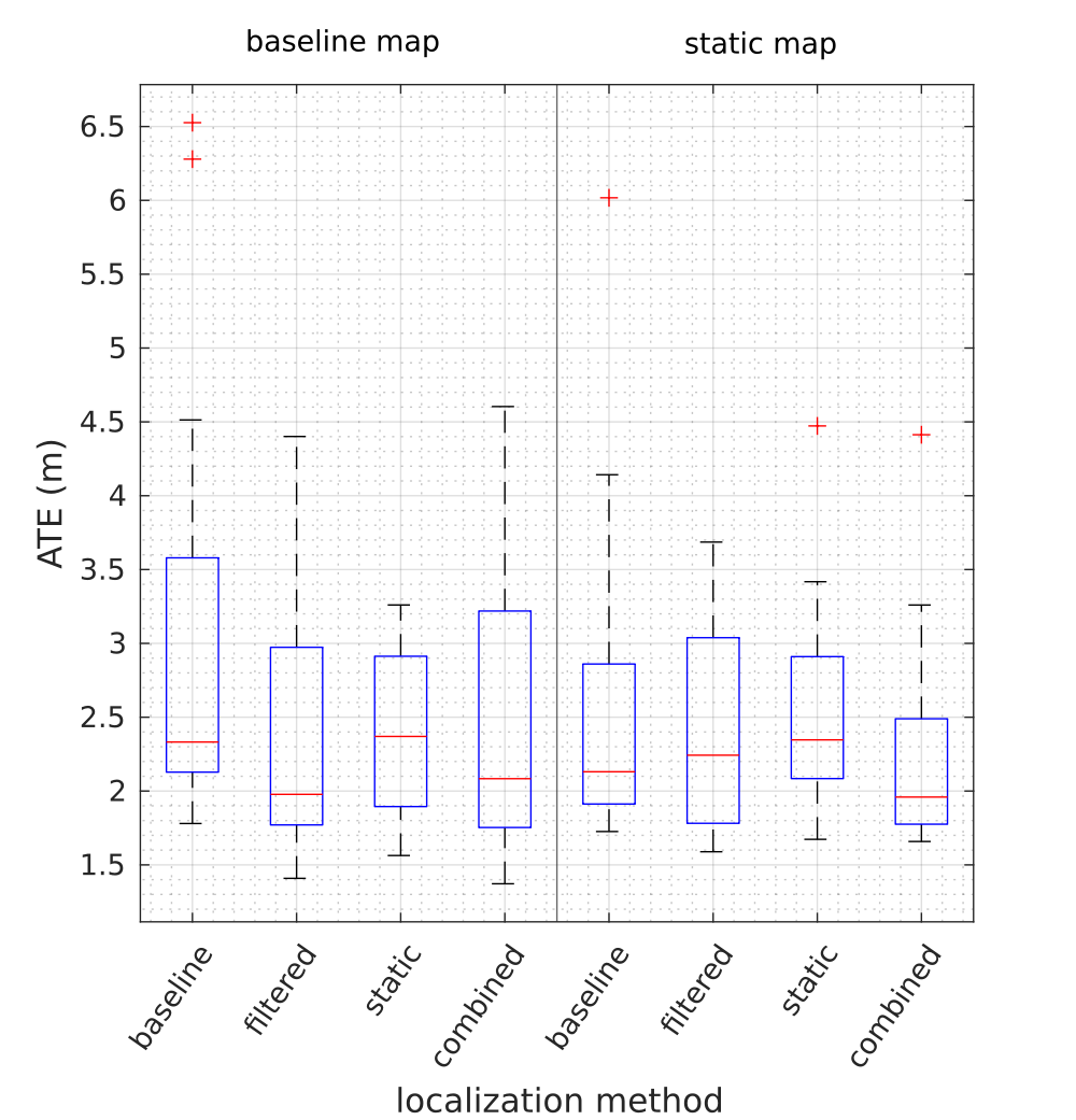
Figure 2: The experiment results. In the figure the sample median is presented with a red line, and the blue box represents the range between 25${}^{\text{th}}$ and 75${}^{\text{th}}$ percentile, i.e., the interquantile range. The black dashed line presents the interval between the minimum and the maximum samples. Values over 1.5 times the interquantile range are marked as outliers, and displayed with a red plus symbol.

TABLE IV: Mean ATEs

localization type	baseline map	static map
baseline	3.0642 m	2.5973 m
filtered	2.3292 m	2.4248 m
static	2.4066 m	2.5681 m
combined	2.4689 m	2.2646 m

TABLE V: Variance of ATEs

localization type	baseline map	static map
baseline	2.5211 m	1.4081 m
filtered	0.7467 m	0.5134 m
static	0.2873 m	0.5647 m
combined	1.1958 m	0.5858 m

TABLE VI: Mean RPEs

localization type	baseline map	static map
baseline	0.6166 m	0.6118 m
filtered	0.6661 m	0.6651 m
static	0.6256 m	0.6239 m
combined	0.6633 m	0.6630 m

TABLE VII: Variance of RPEs

localization type	baseline map	static map
baseline	0.0013 m	0.0012 m
filtered	0.0014 m	0.0014 m
static	0.0011 m	0.0013 m
combined	0.0014 m	0.0012 m

Several conclusions can be drawn from the results in terms of ATE, which are presented in Figure 2 and in Tables V and V.

First, using the static map improves localization accuracy, which can be seen from Figure 2 by comparing the performance of each localization method over the two different types of map. With all method except the static localization, using the static map would be preferable as it reduces variance or improves the mean, or both. With the static localization, the difference between the maps is negligible. This is likely due to the nature of NDT registration, where only matches between measurements and the map contribute to the cost. As there are no cost for unmatched cells, it matters less if the measurements are removed from the measurements or from the map, as the reduction in error is similar.

These results indicate that in three out of the four cases the static map increases the performance, and in one case the performance stays the same. As the static map consists of only static measurements, this result is in concord with the hypothesis that having consistent assumptions over dynamics increases the localization accuracy.

Second, the filtering of the measurements during localization also improves localization accuracy. The results in Figure 2 suggest that dynamic objects may cause large magnitude errors when incorrectly matched with the map. Our experiments showed that filtering dynamic and semi-static objects both decreased the maximum of the errors and removed the large outliers. Compared against the baseline localization, the filtering methods have reduced mean or variance, or both, making them more desirable choices.

Third, in terms of variance, the static localization has the best performance. Whereas the filtered localization can achieve very low errors, the variance is higher than with the static localization. While using more measurements is generally beneficial for the localization accuracy, the incorrect matching of semi-static object may cause errors. This makes the the use of only static objects desirable, as they are the most reliable landmarks.

Given the two main hypotheses: (i) using only static measurements in the map and (ii) the filtering the localization input are both beneficial for the localization accuracy, it should follow that the baseline localization with the baseline map should be the worst performing combination, which can be clearly seen from the results. As the baseline map holds semi-static measurements and the localization uses dynamic measurements, these can be incorrectly matched, reducing performance. Therefore by violating the consistent assumptions over dynamics, the localization accuracy is decreased. Conversely, when the static map and the combined method are used together, the minimum ATE over all of the combinations is achieved.

The means and variances in terms of RPE are presented in Tables VII and VII, respectively. The differences between the different mapping and localization methods are negligible.

The effect of increased temporal distance between the map creation and localization time was studied, but the experiments were inconclusive. This is likely due to the fact that the data set was gathered on very similar time of day with respect to the traffic conditions, namely ranging from 11:46 to 15:20 during weekdays. It is likely that the environment is more similar at the same time of day across different days than between different times of the day on the same day. Therefore a more heterogeneous data set should be acquired to better study the temporal effects.

In conclusion, the results indicate that when both semantic information as well as dynamic information are taken into account, the localization accuracy is increased.

VI Conclusion

In this work, we argue that more realistic assumptions over dynamics are necessary. We showed that violating the static world assumption increases the localization error due to the mismatch between the map and semi-static or dynamic measurements treated as static. We additionally proposed a method to partition measurements according to their dynamic properties through a combination of dynamic object filtering and semantic segmentation. Finally, we used the proposed method to build a mapping-localization framework that is consistent with assumptions over dynamics.

The proposed methods were tested with 112 localization experiments with real-world data gathered over seven different days spanning nine days in a city traffic scenario. The results show that by either using a map only consisting of static measurements or using only static measurements for the localization, or both, the localization error lowered in terms of ATE. More importantly, the variance of the error decreased significantly. While the data set used in this work was gathered in a relatively static urban setting, the proposed methods would likely be even more useful in environments containing more semi-static objects. However, in environments where there are only very few or no static objects, the proposed method must be extended to leverage the measurements from other dynamic classes, without relaxing the consistent assumptions over dynamics.

In conclusion, we showed that localization under consistent assumptions over dynamics increases the localization accuracy in terms of ATE. The results pave a way for new interesting research topics. The use of more realistic models of dynamics could enable localization in more challenging environments, where current methods fail. Whereas in this work we studied only the localization accuracy, the proposed methods could improve performance in other important application areas of mobile robotics, such as mapping and path planning.

References

- [1] D. Fox, W. Burgard, S. Thrun, and A. B. Cremers, “Position Estimation for Mobile Robots in Dynamic Environments,” AAAI/IAAI, vol. 1998, p. 6, 1998.
- [2] D. Hahnel, R. Triebel, W. Burgard, and S. Thrun, “Map building with mobile robots in dynamic environments,” in 2003 IEEE International Conference on Robotics and Automation (ICRA) (Cat. No.03CH37422). Taipei, Taiwan: IEEE, 2003, pp. 1557–1563.
- [3] D. F. Wolf and G. S. Sukhatme, “Mobile Robot Simultaneous Localization and Mapping in Dynamic Environments,” Autonomous Robots, vol. 19, no. 1, pp. 53–65, July 2005.
- [4] R. Kummerle, M. Ruhnke, B. Steder, C. Stachniss, and W. Burgard, “A navigation system for robots operating in crowded urban environments,” in 2013 IEEE International Conference on Robotics and Automation (ICRA). Karlsruhe, Germany: IEEE, May 2013, pp. 3225–3232.
- [5] J. P. Saarinen, H. Andreasson, T. Stoyanov, and A. J. Lilienthal, “3D normal distributions transform occupancy maps: An efficient representation for mapping in dynamic environments,” The International Journal of Robotics Research (IJRR), vol. 32, no. 14, pp. 1627–1644, Dec. 2013.
- [6] X. Chen, A. Milioto, E. Palazzolo, P. Giguère, J. Behley, and C. Stachniss, “SuMa++: Efficient LiDAR-based Semantic SLAM,” in 2019 IEEE/RSJ International Conference on Intelligent Robots and Systems (IROS), Nov. 2019, pp. 4530–4537, arXiv:2105.11320 [cs].
- [7] J. Saarinen, H. Andreasson, T. Stoyanov, and A. J. Lilienthal, “Normal distributions transform Monte-Carlo localization (NDT-MCL),” in 2013 IEEE/RSJ International Conference on Intelligent Robots and Systems (IROS). Tokyo: IEEE, Nov. 2013, pp. 382–389.
- [8] A. Elfes, “Sonar-based real-world mapping and navigation,” IEEE Journal on Robotics and Automation, vol. 3, no. 3, pp. 249–265, June 1987.
- [9] D. Meyer-Delius, J. Hess, G. Grisetti, and W. Burgard, “Temporary maps for robust localization in semi-static environments,” in 2010 IEEE/RSJ International Conference on Intelligent Robots and Systems (IROS). Taipei: IEEE, Oct. 2010, pp. 5750–5755.
- [10] A. Petrovskaya, “Probabilistic Mobile Manipulation in Dynamic Environments, with Application to Opening Doors,” in IJCAI, 2007.
- [11] D. Schulz and W. Burgard, “Probabilistic state estimation of dynamic objects with a moving mobile robot,” Robotics and Autonomous Systems, vol. 34, no. 2-3, pp. 107–115, Feb. 2001.
- [12] G. D. Tipaldi, D. Meyer-Delius, and W. Burgard, “Lifelong localization in changing environments,” The International Journal of Robotics Research (IJRR), vol. 32, no. 14, pp. 1662–1678, Dec. 2013.
- [13] D. Meyer-Delius, M. Beinhofer, and W. Burgard, “Occupancy Grid Models for Robot Mapping in Changing Environments,” Proceedings of the AAAI Conference on Artificial Intelligence (AAAI), vol. 26, no. 1, pp. 2024–2030, Sept. 2021.
- [14] J. Biswas and M. Veloso, “Episodic non-Markov localization: Reasoning about short-term and long-term features,” in 2014 IEEE International Conference on Robotics and Automation (ICRA). Hong Kong, China: IEEE, May 2014, pp. 3969–3974.
- [15] D. M. Rosen, J. Mason, and J. J. Leonard, “Towards lifelong feature-based mapping in semi-static environments,” in 2016 IEEE International Conference on Robotics and Automation (ICRA). Stockholm, Sweden: IEEE, May 2016, pp. 1063–1070.
- [16] A. Zaganidis, A. Zerntev, T. Duckett, and G. Cielniak, “Semantically Assisted Loop Closure in SLAM Using NDT Histograms,” in 2019 IEEE/RSJ International Conference on Intelligent Robots and Systems (IROS). Macau, China: IEEE, Nov. 2019, pp. 4562–4568.
- [17] S. Zhu, X. Zhang, S. Guo, J. Li, and H. Liu, “Lifelong Localization in Semi-Dynamic Environment,” in 2021 IEEE International Conference on Robotics and Automation (ICRA). Xi’an, China: IEEE, May 2021, pp. 14 389–14 395.
- [18] T. Morris, F. Dayoub, P. Corke, and B. Upcroft, “Simultaneous localization and planning on multiple map hypotheses,” in 2014 IEEE/RSJ International Conference on Intelligent Robots and Systems (IROS). Chicago, IL, USA: IEEE, Sept. 2014, pp. 4531–4536.
- [19] W. Maddern, G. Pascoe, C. Linegar, and P. Newman, “1 Year, 1000km: The Oxford RobotCar Dataset,” The International Journal of Robotics Research (IJRR), vol. 36, no. 1, pp. 3–15, 2017.
- [20] A. Geiger, P. Lenz, C. Stiller, and R. Urtasun, “Vision meets robotics: The kitti dataset,” International Journal of Robotics Research (IJRR), 2013.
- [21] Q. Hu, B. Yang, L. Xie, S. Rosa, Y. Guo, Z. Wang, N. Trigoni, and A. Markham, “Randla-net: Efficient semantic segmentation of large-scale point clouds,” Proceedings of the IEEE Conference on Computer Vision and Pattern Recognition (CVPR), 2020.
- [22] J. Behley, M. Garbade, A. Milioto, J. Quenzel, S. Behnke, C. Stachniss, and J. Gall, “SemanticKITTI: A Dataset for Semantic Scene Understanding of LiDAR Sequences,” in Proc. of the IEEE/CVF International Conf. on Computer Vision (ICCV), 2019.
- [23] F. Langer, A. Milioto, A. Haag, J. Behley, and C. Stachniss, “Domain Transfer for Semantic Segmentation of LiDAR Data using Deep Neural Networks,” in Proc. of the IEEE/RSJ Intl. Conf. on Intelligent Robots and System (IROS), 2020.
- [24] T. Stoyanov, J. Saarinen, H. Andreasson, and A. J. Lilienthal, “Normal Distributions Transform Occupancy Map fusion: Simultaneous mapping and tracking in large scale dynamic environments,” in 2013 IEEE/RSJ International Conference on Intelligent Robots and Systems. Tokyo: IEEE, Nov. 2013, pp. 4702–4708.
- [25] Daniel Adolfsson, Henrik Andreasson. Graph map. [Online]. Available: https://gitsvn-nt.oru.se/software/graph_map_public.git
- [26] Daniel Adolfsson. Velodyne pointclou oru. [Online]. Available: https://github.com/dan11003/velodyne_pointcloud_oru.git
- [27] Henrik Andreasson, Todor Stoyanov, Daniel Canelhas, Martin Magnusson, Jari Saarinen, Tomasz Kucner, Malcolm Mielle, Chittaranjan Swaminathan, Daniel Adolfsson. Ndt core. [Online]. Available: https://gitsvn-nt.oru.se/software/ndt_core_public.git
- [28] ——. Ndt tools. [Online]. Available: https://gitsvn-nt.oru.se/software/ndt_tools_public.git
- [29] J. Sturm, N. Engelhard, F. Endres, W. Burgard, and D. Cremers, “A benchmark for the evaluation of RGB-D SLAM systems,” in 2012 IEEE/RSJ International Conference on Intelligent Robots and Systems. Vilamoura-Algarve, Portugal: IEEE, Oct. 2012, pp. 573–580.