The Search for Stability: Learning Dynamics of Strategic Publishers with Initial Documents

Abstract

We study a game-theoretic information retrieval model in which strategic publishers aim to maximize their chances of being ranked first by the search engine while maintaining the integrity of their original documents. We show that the commonly used Probability Ranking Principle (PRP) ranking scheme results in an unstable environment where games often fail to reach pure Nash equilibrium. We propose the Relative Ranking Principle (RRP) as an alternative ranking principle and introduce two families of ranking functions that are instances of the RRP. We provide both theoretical and empirical evidence that these methods lead to a stable search ecosystem, by providing positive results on the learning dynamics convergence. We also define the publishers’ and users’ welfare, demonstrate a possible publisher-user trade-off, and provide means for a search system designer to control it. Finally, we show how instability harms long-term users’ welfare.

1 Introduction

The rapid advancement of information retrieval systems, exemplified by search engines such as Google and Bing, and recommendation systems such as YouTube and Spotify, has reshaped how users interact with the vast digital information landscape. Central to their function is ad-hoc retrieval: ranking documents within a corpus according to their relevance to a user’s query. A key phenomenon in such ecosystems is strategic behaviors from content providers, who modify their web content to improve their ranking in search results, a practice known as search engine optimization (SEO). Such strategies can significantly influence the quality of search results and the user’s experience. This phenomenon has garnered substantial attention, and game-theoretic tools have been increasingly applied to analyze it. Since a ranking scheme induces a game, the task of choosing a ranking scheme is essentially a task of mechanism design, a central field in game theory.

However, to the best of our knowledge, none of the previous game-theoretic models has taken into account the fact that besides optimizing visibility, content providers typically have some ideal, preferred content that they aim to provide. Consequently, publishers make revisions and enhancements to their ideal content in order to attain the top ranking while maintaining the fidelity of their preferred content (hereafter, initial documents). Incorporating the notion of initial documents necessitates the differentiation between the utilities of publishers and users, as opposed to the common assumption in the existing literature that the two are aligned.

Lastly, while the publishers’ strategy space is commonly modeled as a finite set of ”topics” (e.g., [BTK17, RRTK17, BPRT19]), we highlight the fact that free text is better represented as a continuous, high-dimensional space. This high-dimensional space can be thought of as the word embedding of the documents (e.g. [YNL21]), which serves as the input for the ranking function. Alternatively, documents can be represented by a set of higher-level features, which can be learned by the ranking system based on the documents’ content and metadata.

Our contribution

In this paper, we suggest a framework that models the strategy space of publishers as a continuous embedding space, distinguishes between publishers’ and users’ welfare, and accounts for publishers’ initial documents. Within this model, we study the convergence of better response dynamics under different ranking schemes. We provide a negative result on the stability of the widely used Probability Ranking Principle (PRP), a principle that states that documents should be ranked in order of decreasing probability of relevance to the user [Rob77]. We propose the Relative Ranking Principle (RRP) as an alternative. We then introduce two concrete ranking schemes which are instances of the RRP, the softmax RRP and the linear RRP. For the linear RRP, we prove the convergence of any better response learning dynamics to a stable state using a potential function argument. Following this, we empirically demonstrate how the instability of the PRP ranking function harms its performance in relation to the performance of the RRP ranking functions. In addition, we show an inherent trade-off between publishers’ welfare and users’ welfare and provide a means for a system designer to control it.

Note that in practice, a search engine designer is typically interested in designing a ranking scheme that guarantees the convergence of actual dynamics induced by strategic modification of content in the text space. While the structure of such dynamics is unknown, a stronger approach we adopt is to design a ranking scheme that guarantees the convergence of any better response dynamics. This approach in particular ensures the convergence of any real-life dynamics in which the designer might be interested. Although this paper focuses on search engines, our analysis is also applicable to any recommendation-based ecosystem in which content providers are incentivized to optimize visibility by manipulating their content.

The rest of the paper is organized as follows: in Section 2 we review related work in the field of strategic information retrieval. Section 3 provides preliminary definitions and results from game theory, which will be used throughout the paper. In Section 4 we discuss our novel game-theoretic model. Section 5 provides a theoretical analysis of learning dynamics in our model and of the stability of different ranking schemes. In Section 6 we provide experimental results of simulating learning dynamics under the different ranking schemes. We then conclude and present future work directions in Section 7. All proofs, as well as additional in-depth theoretical and empirical analysis of the ranking schemes, are deferred to the appendix.

2 Related Work

Our work lies in the intersection of game theory, economics, and machine learning. There is extensive literature on various strategic and societal aspects of machine learning, such as classification and segmentation of strategic individuals [HMPW16, NST18, LR22, NGTCR22], fairness in machine learning [CKLV17, ABV21, BPST21], and recommendation systems design [BPT18, BPGRT19, BBPLBT20, MCBP⁺20].

In this work, we study a game-theoretic model of the search (or more generally, recommendation) ecosystem, in which strategic content providers compete to maximize impressions and visibility. [BBTK15, BTK17] showed that the widely used PRP ranking scheme of [Rob77] leads to sub-optimal social welfare, and demonstrated how introducing randomization into the ranking function can improve social welfare in equilibrium. [RRTK17] provided both theoretical and empirical analysis of a repeated game, and revealed a key strategy of publishers: gradually making their documents become similar to documents ranked the highest in previous rounds. [KT22] advocates for the devising of ranking functions that are optimized not only for short-term relevance effectiveness but also for long-term corpus effects.

In this paper, we focus on studying the learning dynamics of publishers in our model. We utilize a result of [MS96] on the convergence of any better response dynamics for the class of potential games. This class of games is known to be equivalent to the class of congestion games [Ros73]. [Mil96] introduced another class of games in which learning dynamics always converge to a pure Nash equilibrium.

Learning dynamics are well studied in the context of machine learning, data-driven environments, recommendation systems, and ad auctions [CB98, FS99, MPRJ10, CDE⁺14]. In particular, the convergence of learning dynamics is considered an important property, indicating the stability of the search ecosystem [BPRT19].

3 Preliminaries

In this section, we provide some standard definitions and results from the field of game theory. We start with the definition of a game:

Definition 1.

An $n$-player game is a tuple $G=\bigl{(}N,(X_{i})_{i\in N},(u_{i})_{i\in N}\bigr{)}$, where $N\coloneqq\{1,...,n\}$ is the set of players, and for each player $i\in N$, $X_{i}$ is the set of actions. The set $X\coloneqq X_{1}\times...\times X_{n}$ is called the set of pure strategy profiles. Each player $i\in N$ has a utility function $u_{i}:X\to\operatorname*{\mathbb{R}}$.

Throughout the paper, we assume that $X_{i}$ is a compact and convex set and that $u_{i}$ is a bounded function for all $i\in N$. We also assume that all players are rational, in the sense that each player attempts to maximize her own utility. Each player’s utility depends not only on her action but also on the actions taken by all other players. We denote by $X_{-i}\coloneqq X_{1}\times...\times X_{i-1}\times X_{i+1}\times...\times X_{n}$ the set of all pure strategy profiles of all players but player $i$, and use the notation of $x_{-i}\in X_{-i}$ to denote such a strategy profile of everyone but $i$. An important concept is the concept of $\varepsilon$-better response.

Definition 2.

Given a pure strategy profile $x_{-i}\in X_{-i}$ of all players but player $i$ and actions $x_{i},\;x^{\prime}_{i}\in X_{i}$ of player $i$, we say $x^{\prime}_{i}$ is an $\varepsilon$-better response than $x_{i}$ with respect to $x_{-i}$ if $u_{i}(x^{\prime}_{i},x_{-i})>u_{i}(x_{i},x_{-i})+\varepsilon$.

The notion of $\varepsilon$-best response allows defining the solution concept of an $\varepsilon$-pure Nash equilibrium: a pure strategy profile from which no player can improve her utility by more than $\varepsilon$ by deviating (i.e., changing her actions given all other players’ actions are fixed).

Definition 3.

A pure strategy profile $x\in X$ is called an $\varepsilon$-pure Nash equilibrium ($\varepsilon$-PNE), if for every player $i\in N$, no $x^{\prime}_{i}$ is an $\varepsilon$-better response than $x_{i}$ with respect to $x_{-i}$.

For $\varepsilon=0$, $0$-PNE and $0$-better response are called PNE and better response, respectively. A PNE is often considered a stable state of a game (e.g., [BPT18]). While in general games its existence is not guaranteed, some classes of games always possess a PNE. We say a game $G$ is smooth if, for each $i\in N$, $u_{i}$ has continuous partial derivatives with respect to the components of $x_{i}$. The following is a well-known fact that can be derived from [Nag98]:

Lemma 1.

Any smooth game possesses a PNE.

When players apply the concept of $\varepsilon$-better response we get the following type of dynamics:

Definition 4.

An $\varepsilon$-better response dynamics is a sequence of profiles $\bigl{\{}x^{(t)}\bigr{\}}_{t=1}^{\infty}\subseteq X$ such that in each timestep $t$ either $x^{(t-1)}$ is an $\varepsilon$-PNE and $x^{(t)}=x^{(t-1)}$ or there is a single deviator $i\in N$ such that:

• $x^{(t)}_{-i}=x^{(t-1)}_{-i}$

• $x^{(t)}_{i}$ is an $\varepsilon$-better response than $x^{(t-1)}_{i}$ with respect to $x^{(t-1)}_{-i}$.

We say such a dynamics has converged if there exists a timestep $T$ such that $x^{(T)}$ is an $\varepsilon$-PNE.

Another class of games, which will be of interest in this paper, is the class of potential games, presented in [MS96].

Definition 5.

(Monderer and Shapley, 1996) A game $G$ is called a potential game (also known as an exact potential game) if there exists a potential function (also known as a potential) $\phi:X\to\operatorname*{\mathbb{R}}$, such that for any $i\in N,x_{-i}\in X_{-i},x^{\prime}_{i},x^{\prime\prime}_{i}\in X_{i}$:

$$\phi(x^{\prime}_{i},x_{-i})-\phi(x^{\prime\prime}_{i},x_{-i})=u_{i}(x^{\prime}_{i},x_{-i})-u_{i}(x^{\prime\prime}_{i},x_{-i})$$

That is, in a potential game, a single function $\phi$ ”captures” the incentives of all the players. It is straightforward that any potential maximizer is a PNE. Moreover, [MS96] shows a significant result:

Theorem 1.

(Monderer and Shapley, 1996) Let $G$ be an exact potential game and let $\varepsilon>0$. Then, $G$ possesses at least one $\varepsilon$-PNE, and any $\varepsilon$-better response dynamics in $G$ converges.

Another important concept is the concept of a strictly dominant strategy, a strategy which is the best choice for a player regardless of the strategies chosen by other players. The significance of strictly dominant strategies lies in their stability and predictability.

Definition 6.

We say that a strategy $x_{i}\in X_{i}$ strictly dominates strategy $x^{\prime}_{i}\in X_{i}$ (or: $x^{\prime}_{i}$ is strictly dominated by $x_{i}$) if for every strategy profile of the other publishers $x_{-i}\in X_{-i}$, $x_{i}$ is a better response than $x^{\prime}_{i}$ with respect to $x_{-i}$.
A strategy $x_{i}\in X_{i}$ is called a strictly dominant strategy if it dominates any other strategy of player $i$.
A strategy $x_{i}\in X_{i}$ is called a strictly dominated strategy if it is strictly dominated by another strategy of player $i$.

4 The Model

We start by defining the basic model of a publishers’ game. A publishers’ game consists of $n$ publishers (players), each can provide content in the continuous $k$-dimensional space $[0,1]^{k}$, where distance between documents is measured by some continuous semi-metric $d$. Each publisher $i$ has a preferred content type (or: initial document), denoted by $x_{0}^{i}\in[0,1]^{k}$. We denote by $x^{*}\in[0,1]^{k}$ the desirable information need representation in the feature space. In our model, the information need is represented in the same embedding space as the documents, inspired by models of BERT rankers and dense retrieval (e.g., [QXLL19, ZML⁺20, ZLRW22]). The term $x^{*}$ can be used to refer to a particular query or topic in the search environment. The search engine uses some ranking function $r$ to determine the documents’ ranking. We assume that $r$ is oblivious, meaning it is independent of the publishers’ identities. Formally:

Definition 7.

A publishers’ game is a tuple $G=(N,k,(X_{i})_{i\in N},\lambda,d,(x_{0}^{i})_{i\in N},x^{*},r)$, where:

• $N\coloneqq\{1,2,...n\}$ is the set of publishers, with $n\geq 2$;

• $k$ is the embedding-space dimension of documents;

• $\forall i\in N:X_{i}\coloneqq[0,1]^{k}$ is the set of possible actions for publisher $i$;

• $\lambda>0$ is the factor of the cost for providing content that is different from the initial document;

• $d:[0,1]^{k}\times[0,1]^{k}\to\operatorname*{\mathbb{R}}_{+}$ is a continuous semi-metric satisfying $\forall x,y:d(x,y)\leq 1$;

• $\forall i\in N:x_{0}^{i}\in X_{i}$ is the initial document of publisher $i$;

• $x^{*}\in[0,1]^{k}$ is the information need;

• $r:X\to\Delta^{n}$ is a ranking function, that might depend on the information need $x^{*}$.

The ranking function $r$ determines the distribution over the winning publishers given a strategy profile $x\in X$, with the interpretation that $r_{i}(x)$ is the probability of publisher $i$ being ranked first by $r$ under the strategy profile $x$. We abuse the notation and denote $d^{*}(x_{i})\coloneqq d(x_{i},x^{*})$ and $d^{0}_{i}(x_{i})\coloneqq d(x_{i},x_{0}^{i})$. We also define the function $\vec{d^{*}}:X\to[0,1]^{n}$ as $\vec{d_{i}^{*}}(x)\coloneqq d^{*}(x_{i})$. The utility of publisher $i$ under the profile $x$ is then defined to be:

$$u_{i}(x)\coloneqq r_{i}(x)-\lambda d^{0}_{i}(x_{i})$$

That is, the utility of publisher $i$ is the probability of winning minus the cost of providing content that differs from her initial document. Then we define the publishers’ welfare to be the social welfare (the sum of the utilities of all the players) of the publishers’ game, i.e.:

$$\mathcal{U}(x)\coloneqq\sum_{i=1}^{n}u_{i}(x)=1-\lambda\sum_{i=1}^{n}d^{0}_{i}(x_{i})$$

In addition, we define another type of welfare, the users’ welfare:

$$\mathcal{V}(x)\coloneqq\sum_{i=1}^{n}\bigl{(}1-d^{*}(x_{i})\bigr{)}\cdot r_{i}(x)=1-\sum_{i=1}^{n}d^{*}(x_{i})\cdot r_{i}(x)$$

That is, the users’ welfare is the expected relevance of the first-ranked document, where we quantify the relevance of a document $x_{i}$ by $1-d^{*}(x_{i})$. We will henceforth use the term welfare measures to collectively refer to both publishers’ welfare and users’ welfare.

5 Ranking Functions and Learning Dynamics

In this section, our aim is to provide a game-theoretic analysis of learning dynamics in our model and discuss different ranking schemes. We consider the convergence of any $\varepsilon$-better response dynamics as a desirable property of ranking functions, indicating stability and predictability. We begin by showing that the well-known Probability Ranking Principle (PRP) induces an unstable game in which publishers’ learning dynamics may fail to converge to a pure Nash equilibrium. Then, we propose a novel alternative principle for ad-hoc retrieval and two concrete ranking functions that follow the suggested approach.

5.1 The PRP Ranking Function

The Probability Ranking Principle (PRP) [Rob77] is a key principle in information retrieval, which forms the theoretical foundations for probabilistic information retrieval. The principle says that documents should be ranked in decreasing order of the probability of relevance to the information need expressed by the query. In our model, the analogous principle means that the document that is the closest to the information need should always be ranked first by the ranking function. We begin with formally defining the PRP ranking function in our model:

Definition 8.

The PRP ranking function, denoted by $r^{*}$, is the ranking function defined as follows:

$$r_{i}^{*}(x)\coloneqq\begin{cases}\frac{1}{|\mu(x)|}&i\in\mu(x)\\ 0&i\notin\mu(x)\end{cases}$$

where $\mu(x)\coloneqq\operatorname*{argmin}_{i\in N}d^{*}(x_{i})$ is the set of all publishers providing the closest content to the information need $x^{*}$.

Note that the PRP yields optimal short-term retrieval in the sense that for a fixed strategy profile $x$, the PRP ranking function maximizes the users’ welfare $\mathcal{V}(x)$. However, its discontinuity induces an unstable ecosystem, in which there might not exist a PNE. This instability causes sub-optimal long-term effects, as we show later.

Observation 1.

Let $k\in\operatorname*{\mathbb{N}}$ and let $G$ be a publishers’ game with $n=2$, $\lambda>\frac{1}{2}$, $d(x,y)=\frac{1}{k}\left\lVert x-y\right\rVert^{2}_{2}$, $r=r^{*}$, $x_{0}^{1}=x_{0}^{2}=\vec{0}_{k}$ and $x^{*}=\vec{1}_{k}$. Then, $G$ possesses no PNE.

The presence of a pure Nash equilibrium holds significant importance for search engine designers. We now turn to suggest an alternative ranking principle, which will lay the foundations for two alternative ranking functions. These ranking functions will be shown (either theoretically or empirically) to be stable in terms of PNE existence and $\varepsilon$-better response dynamics convergence.

5.2 The Relative Ranking Principle

The Probability Ranking Principle suggests ranking the documents according to the same order induced by their probabilities of relevance with respect to the information need (or, in our model, with respect to the distance from the information need in the embedding space). In the previous section, we have shown that the PRP ranking function induces an unstable publishers’ game, which calls for alternative ranking principles. As demonstrated in the proof of Observation 1, the cause for this instability is the non-continuous nature of the PRP ranking function. Therefore, we suggest taking a smooth variation of the Probability Ranking Principle, which we call the Relative Ranking Principle (RRP). The principle posits two key conditions: (1) the ranking function should be continuously differentiable with respect to the distances from $x^{*}$, and (2) for any given publisher, the probability of being ranked first should be strictly decreasing in her distance from the information need and strictly increasing in the distance of any other publisher from the information need. A formal definition would be:

Definition 9.

A ranking function $r$ is a Relative Ranking Principle (RRP) ranking function if there exists a continuously differentiable function $m:[0,1]^{n}\to\Delta^{n}$ such that the following conditions hold:

1. $r=m\circ\vec{d^{*}}$

2. For every two publishers $i\neq j\in N,\frac{\partial m_{i}}{\partial d_{i}}<0$ and $\frac{\partial m_{i}}{\partial d_{j}}>0$.

Note that the PRP ranking function does not satisfy either of the two requirements of the RRP principle. An immediate result from Lemma 1 is that whenever $d$ is continuously differentiable, which is indeed the case for many natural semi-metrics, all RRP ranking functions induce a game that possesses at least one PNE. We now turn to introduce two ranking functions families, which are instances of the RRP.

5.3 The Softmax RRP Ranking Functions

Since the discontinuity of the PRP, which leads to its instability, is caused by the discontinuity of the argmax function, a natural way to construct a smooth version of the PRP would be to replace the argmax function with its well-known smooth approximation - the softmax function. It is worth discussing the resulting ranking functions, even though the theoretical results presented here concerning them are not positive, due to their remarkable empirical performance, detailed in Section 6.

Definition 10.

The softmax function with inverse temperature constant $\beta>0$ is the function $\sigma^{\beta}:\operatorname*{\mathbb{R}}^{n}\to\Delta^{n}$ given by

$$\sigma^{\beta}_{i}(y)\coloneqq\frac{e^{\beta y_{i}}}{\sum_{j=1}^{n}e^{\beta y_{j}}}$$

Definition 11.

The softmax RRP ranking function with inverse temperature constant $\beta>0$, denoted by $\tilde{r}^{\beta}$, is the ranking function defined as follows:

$$\tilde{r}^{\beta}\coloneqq\sigma^{\beta}\circ\bigl{(}-\vec{d^{*}}\bigr{)}$$

Note that as $\beta\to\infty$, $\tilde{r}^{\beta}\to r^{*}$. This further explains the intuition behind the usage of the softmax function in our context and shows that $\beta$ is a means to control how closely the softmax ranking function aligns with the PRP. The softmax RRP ranking functions are all members of a wider ranking functions family - the proportional RRP ranking functions. The proportional RRP condition is an intuitive way to construct a function whose image is contained in the simplex $\Delta^{n}$.

Definition 12.

We say a ranking function $r$ is a proportional RRP ranking function if there exists a continuously differentiable and strictly decreasing function $g:[0,1]\to\operatorname*{\mathbb{R}}_{++}$ such that

$$r_{i}(x)=\frac{g\bigl{(}d^{*}(x_{i})\bigr{)}}{\sum_{j=1}^{n}g\bigl{(}d^{*}(x_{j})\bigr{)}}$$

We say a ranking function $r$ induces a potential game if any publishers’ game with $r$ as its ranking function is a potential game.

Theorem 2.

There exists no proportional RRP ranking function that induces a potential game.

Theorem 2 implies in particular that the softmax RRP ranking function does not induce a potential game. This negative result motivates the study of linear ranking functions, presented in the following subsection.

5.4 The Linear RRP Ranking Functions

Before introducing the linear RRP ranking functions, we start by defining the linear relative relevance:

Definition 13.

Let $x\in X$ be a strategy profile in a publishers’ game. The linear relative relevance of document (or publisher) $i\in N$ with respect to $x$ is:

$$\nu_{i}(x)\coloneqq\frac{1}{n-1}\Bigl{(}\sum_{j\in N\setminus\{i\}}d^{*}(x_{j})\Bigr{)}-d^{*}(x_{i})$$

That is, the linear relative relevance is the difference between the average distance of all other publishers from the information need and the distance of publisher $i$’s document from the information need. Our next step is characterizing the set of all RRP ranking functions which are linear transformations of the linear relative relevance.

Lemma 2.

Denote by $\hat{r}^{a,b}$ the function satisfying $\hat{r}^{a,b}_{i}(x)=a\cdot\nu_{i}(x)+b$ for every strategy profile $x\in X$. Then, $\hat{r}^{a,b}$ is a valid RRP ranking function if and only if $a\in(0,\frac{1}{n}]$ and $b=\frac{1}{n}$.

Let us denote $\hat{r}^{a}\coloneqq\hat{r}^{a,\frac{1}{n}}$ and refer to $\{\hat{r}^{a}\}_{a\in(0,\frac{1}{n}]}$ as the linear RRP ranking functions. The following main result shows an appealing property of the linear ranking functions.

Theorem 3.

Let $a\in(0,\frac{1}{n}]$. $\hat{r}^{a}$ induces a potential game, and the following is a potential function:

$$\hat{\phi}(x)=-\sum_{i=1}^{n}\bigr{(}a\cdot d^{*}(x_{i})+\frac{1}{n}+\lambda d^{0}_{i}(x_{i})\bigl{)}$$

The following result follows from Theorem 1 and from the continuity of the potential:

Corollary 1.

Let $a\in(0,\frac{1}{n}]$. Any publishers’ game with $r=\hat{r}^{a}$ has at least one PNE. Moreover, for any $\varepsilon>0$, any $\varepsilon$-better response dynamics converges.

The above corollary has major implications regarding the stability of the content providers ecosystem. Specifically, if any $\varepsilon$-better response dynamics converge, then, in particular, any real-life better response dynamics converge. The result regarding learning dynamics convergence does not require full information of the initial documents of all players, but only assumes each player knows her initial document and the information need. Note that whenever $d$ is strictly biconvex, i.e. $d(x,y)$ is strictly convex in $x$ for any fixed $y$ and vice versa (which is the case for semi-metrics like squared Euclidean norm), $\hat{\phi}$ is strictly concave. Together with the unique structure of the linear ranking function, this allows the derivation of the following theorem:

Theorem 4.

Let $a\in(0,\frac{1}{n}]$. If $d$ is strictly biconvex, then any publishers’ game with $r=\hat{r}^{a}$ has a unique PNE and any publisher’s equilibrium strategy is a strictly dominant strategy.

The theorem shows that whenever $d$ is strictly biconvex, not only that the linear RRP possesses the strong behavioral property that any $\varepsilon$-better response learning dynamics converges, the resulting strategies are strictly dominant strategies for the publishers. From now on, we focus our theoretical analysis on $\hat{r}\coloneqq\hat{r}^{\frac{1}{n}}$. The choice $a=\frac{1}{n}$ is rather natural since increasing the slope $a$ amplifies the influence of the documents on the ranking. A similar analysis can be made for other slopes. The following Lemma provides a characterization of the unique equilibrium point in the case of the squared Euclidean distance function.

Lemma 3.

Any publishers’ game with $r=\hat{r}$ and $d(x,y)=\frac{1}{k}||x-y||^{2}_{2}$ has a unique PNE, $x^{eq}$, given by $x^{eq}_{i}=\frac{x^{*}+\lambda nx_{0}^{i}}{1+\lambda n}$. Moreover, $x^{eq}_{i}$ is a strictly dominant strategy for any publisher $i\in N$.

Note that the equilibrium strategy of each publisher is a weighted average of her initial document and $x^{*}$. The closed form of the PNE enables us to analyze how the game parameters affect the welfare measures in equilibrium. For example, deriving the publishers’ welfare in equilibrium by $\lambda$ reveals that it has a global minimum in $\lambda=\frac{1}{n}$. It decreases in $\lambda$ for $\lambda\leq\frac{1}{n}$ and increases for $\lambda\geq\frac{1}{n}$. As for the users’ welfare, under a regularity condition regarding $x_{0}$ and $x^{*}$, we get that it decreases in $\lambda$. Rigorous analysis is available within Appendix B. Although it may seem possible to generalize linear RRP ranking functions by composing a nonlinear function on the linear relative relevance, we prove that this is impossible.

Theorem 5.

The only RRP ranking functions of the form $r_{i}(x)=g\big{(}\nu_{i}(x)\big{)}$ for some $g:[-1,1]\to\operatorname*{\mathbb{R}}$ are the linear RRP ranking functions.

6 Empirical Results

In this section, we evaluate the performance of the PRP, the linear RRP, and the softmax RRP ranking functions in simulated environments that aim to reflect realistic better response dynamics. Empirical analysis of competitive retrieval settings is a difficult challenge, as discussed in [KT22]. Conducting experiments using real data requires the implementation of each proposed ranking function into real systems, in which publishers/content creators repeatedly compete for exposure and receive feedback from a system that ranks according to the proposed approach. Therefore we evaluate our ranking functions using a code-simulated environment which we call the Discrete Better Response Dynamics Simulation. These dynamics are typical in real-world scenarios, where publishers endeavor to enhance the visibility and impressions of their content within the platform they operate. In this section, we focus on the commonly observed case where $n=2$, meaning that two prominent publishers compete for search engine impressions.

Data: $G,\mathcal{S},\mathcal{D},T,M,\epsilon$

$x^{(0)}\leftarrow x_{0}$;

$conv\leftarrow False$;

for $t=1,2,...T$ do

       $\mathcal{I}\leftarrow\bigl{\{}i:\exists(s,d)\in\mathcal{S}\times\mathcal{D}$ s.t. $(x^{(t-1)}_{i}+s\cdot d)\in X_{i}\text{ and }u_{i}\bigl{(}x^{(t-1)}_{i}+s\cdot d,\;x^{(t-1)}_{-i}\bigr{)}>u_{i}\bigl{(}x^{(t-1)}\bigr{)}+\varepsilon\bigr{\}}$;

       if  $\mathcal{I}\neq\emptyset$ then

             Draw $i\in\mathcal{I}$ uniformly;

             Draw $(s^{\prime},d^{\prime})\in\underset{{(s,d)\in\mathcal{S}\times\mathcal{D}}}{\operatorname*{argmax}}\Bigl{\{}u_{i}\bigl{(}x^{(t-1)}_{i}+s\cdot d,\;x^{(t-1)}_{-i}\bigr{)}:\;(x^{(t-1)}_{i}+s\cdot d)\in X_{i}\Bigr{\}}$ uniformly;

             $x^{(t)}\leftarrow\bigl{(}x_{i}^{(t-1)}+s^{\prime}\cdot d^{\prime},\;x_{-i}^{(t-1)}\bigr{)}$;

            

       end if

      else

             $conv\leftarrow True$;

             return $\bigg{(}\mathcal{U}(x^{(t-1)}),\;\mathcal{V}(x^{(t-1)}),\;conv\bigg{)}$;

            

       end if

      

end for

return $\biggr{(}\text{Avg }\bigl{\{}\mathcal{U}(x^{(t)})\bigr{\}}_{t=T-M+1}^{T},\;\text{Avg }\bigl{\{}\mathcal{V}(x^{(t)})\bigr{\}}_{t=T-M+1}^{T},\;conv\biggl{)}$;

Algorithm 1 Discrete Better Response Dynamics Simulation

6.1 Simulation Details

In the Discrete Better Response Dynamics Simulation, we consider dynamics in which publishers are starting with their initial documents, and at each timestep, one publisher modifies her document to improve her utility. The modification is done by taking a step that maximizes the publisher’s utility, from a predefined subset of possible directions $\mathcal{D}$ and step sizes $\mathcal{S}$. Formally, in each simulation, we consider a publishers’ game $G$ with $n=2$, $k=2$, $\lambda\in[0,1]$, $d(x,y)=\frac{1}{k}||x-y||_{2}^{2}$ and uniformly drawn $x^{*}\in[0,1]^{k}$ and $x_{0}\in[0,1]^{n\cdot k}$. A Discrete Better Response Dynamics Simulation is said to converge if it has reached a profile that is an $\varepsilon$-PNE under the discreteness constraints (the constraints of predefined directions and step sizes) within no more than $T$ iterations.

To evaluate the performance of the different ranking functions, we have estimated the convergence rate and the expected long-term publishers’ and users’ welfare. In case the simulation converged, we estimate the welfare measures over the long term using the welfare measures of the profile the simulation converged to. Otherwise, we estimate the welfare measures by averaging them over the last $M$ rounds of the simulation, where $M$ is an additional simulation parameter. A justification for this estimation method is the empirically-observed periodic nature of the dynamics that did not converge. For each value of $\lambda$, we performed multiple simulations and constructed bootstrap confidence intervals with a confidence level of 95%. We introduce the pseudo-code of a single simulation in Algorithm 1.

6.2 Simulations Results

Comparison of the PRP and RRP ranking functions

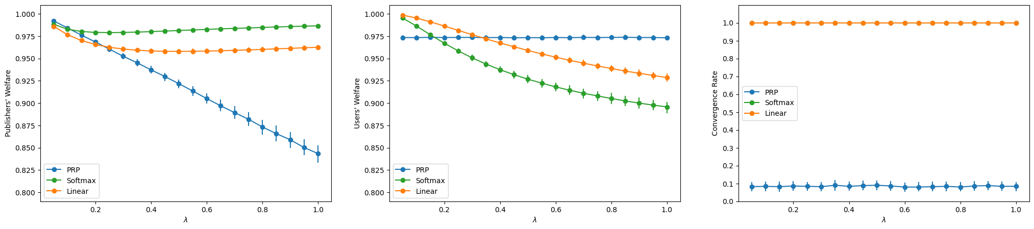
Figure 1: Comparison of the PRP, softmax RRP ($\beta=1$) and linear RRP ($a=\frac{1}{n}=0.5$) ranking functions. The linear RRP and the softmax RRP ranking functions had a constant convergence rate of $1$.

Figure 1 provides a comparative analysis of the PRP ranking function, the softmax RRP with $\beta=1$, and the linear RRP with $a=\frac{1}{n}$. The rightmost chart in Figure 1 highlights a fundamental shortcoming of the PRP ranking function - most of the dynamics it induces do not converge. Both RRP ranking functions, however, have a convergence rate of $1$. This is a key advantage of the RRP ranking functions.

Another insight from Figure 1 is that the users’ welfare of the PRP is roughly constant across $\lambda$ values. A plausible explanation is that in the case of PRP and the tested $\lambda$ range, $\lambda$ has little, if any, impact on the behavior of publishers. This conjecture might also explain why the publishers’ welfare of the PRP appears to linearly decrease with $\lambda$: the dynamics remain the same, but the term $-\lambda\cdot\sum_{i=1}^{n}d^{0}_{i}(x_{i})$ in the publishers’ welfare gains more influence as $\lambda$ increases. Note that the PRP ranking function appears to sacrifice stability in pursuit of increased users’ welfare.

In the linear RRP, the effect of $\lambda$ on the welfare measures matches the theoretical results presented in Subsection 5.4 - the publishers’ welfare obtains a minimum in $\lambda=\frac{1}{n}$, and the users’ welfare is monotonically decreasing in $\lambda$. Another observation from Figure 1 is that the softmax RRP exhibits similar trends. In this figure, an inherent trade-off in our model can be seen - an increase in the publishers’ welfare leads to a decrease in the users’ welfare and vice versa.

One can claim that Figure 1 shows that the linear RRP has higher users’ welfare and lower publishers’ welfare than the softmax RRP. However, tuning the slope $a$ of the linear function and the inverse temperature constant $\beta$ of the softmax function can change this. We now proceed to provide an empirical analysis of the influence of those two hyper-parameters.

The effect of RRP ranking functions hyperparameters

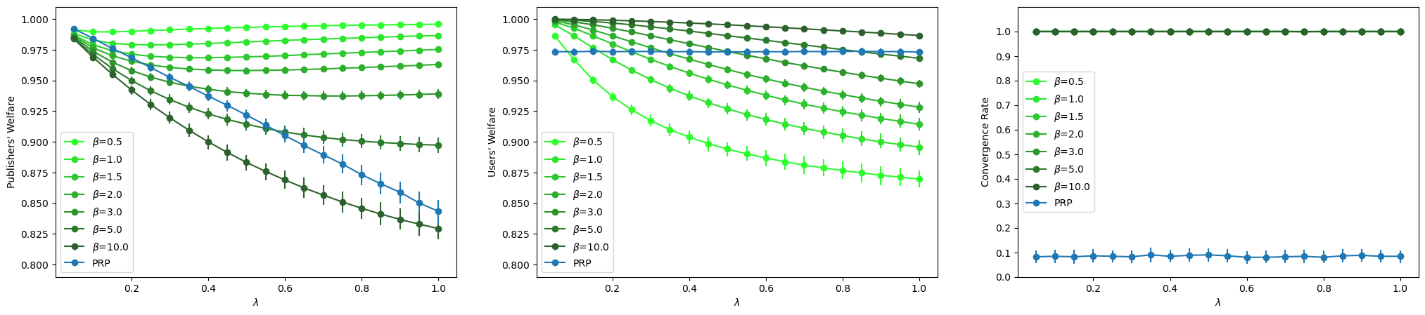
Figure 2: The effect of the inverse temperature constant $\beta$ in the softmax RRP ranking function. All softmax ranking functions had a constant convergence rate of $1$.

Figure 2 provides a comparative analysis of the influence of the inverse temperature constant $\beta$ in the softmax RRP function. It is evident that $\beta$ serves as a means to control the inherent trade-off between publishers’ welfare and users’ welfare. A search engine designer can tune $\beta$ according to the relative importance of users’ and publishers’ welfare within her domain and according to her estimation of $\lambda$. Importantly, the convergence rate of $\tilde{r}^{\beta}$ is $1$ for all tested values of $\beta$. Therefore, the softmax RRP with high $\beta$ values (e.g., $\beta\in\{5,10\}$) manages to surpass the PRP in terms of users’ welfare while maintaining the desired property of $100\%$ convergence. The cost is sacrificing publishers’ welfare. Therefore we claim that the softmax RRP ranking functions offer viable alternatives to the PRP function.

As mentioned in Section 5, the PRP ranking function maximizes the users’ welfare for a fixed profile. The reason why softmax ranking functions with high $\beta$ values nevertheless manage to achieve higher users’ welfare than the PRP is that the PRP is only short-term optimal, while the softmax RRP preserves high users’ welfare on the longer term as well. Unlike the softmax ranking functions, most of the dynamics the PRP induces do not converge. In such ecosystems, the publishers repeatedly reach profiles with sub-optimal users’ welfare, and this harms the long-term users’ welfare of the PRP. This emphasizes the need for the search for stability.

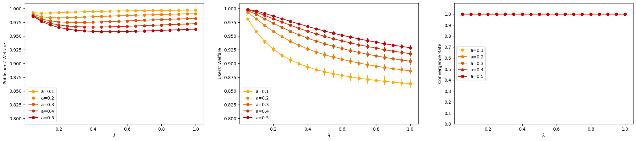
Figure 3: The effect of the slope $a$ in the linear RRP ranking function. All linear ranking functions had a constant convergence rate of $1$.

Now let us delve deeper into the linear ranking function family and compare it to the softmax family. Figure 3 provides a comparative analysis of the influence of the slope $a$ in the linear RRP function. As was the case for the softmax ranking function, $\hat{r}^{a}$ has a convergence rate of $1$ for all tested $a$ values. This result is not surprising, as we proved it in Corollary 1.

Just like $\beta$ in the softmax functions, the slope $a$ allows the search engine designer to control the publisher-user trade-off. There is, however, a core difference between the tuning of $a$ and $\beta$. While the range of $a$ values for which $\hat{r}^{a}$ is a valid RRP ranking function is limited to $(0,\frac{1}{n}]$ (see Lemma 2), one can set the $\beta$ values to be arbitrarily large. This means that using the softmax RRP it is possible to achieve high users’ welfare values that cannot be obtained using the linear RRP. Nevertheless, the linear still has a significant advantage - it induces a potential game. As shown in Subsection 5.4, the potential function enables rigorous theoretical analysis and implies the provable convergence of $\varepsilon$-better response dynamics.

7 Discussion

In this paper, we have suggested a novel game-theoretic model for information retrieval, which models documents as vectors in a continuous space, accounts for original content and distinguishes between publishers’ and users’ welfare. We have provided both theoretical and empirical negative results about the stability of ecosystems in which the PRP principle is used to rank the documents in the corpus and demonstrated how instability harms long-term users’ welfare. Driven by the search for stability, we suggested an alternative approach for ad-hoc retrieval, the Relative Ranking Principle (RRP). While all RRP ranking functions are guaranteed to possess at least one pure Nash equilibrium, we rather focus on a stronger criterion for stability which is the convergence of better response dynamics. We suggest two families of concrete RRP functions: the softmax RRP ranking functions and the linear RRP ranking functions. While we only proved the convergence of any $\varepsilon$-better response dynamics for the linear RRP, both RRP ranking functions have been shown empirically to induce stable ecosystems. The convergence of any $\varepsilon$-better response dynamics in games induced by the linear RRP ranking function is a critical finding, as such dynamics mirror the competitive landscape observed in the real world among publishers. Moreover, we empirically showed an inherent trade-off between publishers’ welfare and users’ welfare and provided means for a search engine designer to control it.

We conclude by stating some key assumptions in our model, as well as limitations of the experimental analysis, which can motivate several interesting future directions. We assumed a specific form of the publishers’ utilities (profit minus cost) and publishers’ full knowledge of the ranking function and the information need. Additionally, we experimented with a specific dynamics structure and narrowed our attention to specific distance functions. Furthermore, another major limitation in the experimental setting is the restriction of uniformly i.i.d distributing $x_{0}$ and $x^{*}$. While the relaxation of some of the assumptions is straightforward (e.g., extending our model to multiple information needs, heterogeneous $\lambda$ values and general cost functions), others require careful analysis and may lead to interesting future research direction. For example, introducing uncertainty regarding the information need would be an interesting avenue for future research. Further, validating our findings via real behavioral data, such as SEO competition data, is another significant research direction.

Appendix A Equilibrium Analysis with the Euclidean Norm

In this section, we provide an equilibrium analysis of publishers’ games that are based on the Euclidean norm, that is, publishers’ games with $d(x,y)=\frac{1}{\sqrt{k}}\left\lVert x-y\right\rVert_{2}$. For each player $i\in N$, we define $L_{i}$ as the line segment that connects the points $x_{0}^{i}$ (her initial document) and $x^{*}$ (the information need). Formally, $L_{i}$ is defined as $L_{i}\coloneqq\{tx^{*}+(1-t)x_{0}^{i}:t\in[0,1]\}$. We use the notation $P_{L_{i}}(x_{i})$ for the projection of $x_{i}$ on $L_{i}$.

Lemma 4.

Let $d$ be a function of the form $d(a,b)=\frac{\left\lVert a-b\right\rVert^{p}}{C}$ for some $C>0$ and $p\geq 1$, where $\left\lVert\cdot\right\rVert$ is the Euclidean ($L_{2}$) norm. Let $G$ be a publishers’ game with $d$ as its semi-metric and whose ranking function is either the PRP ranking function or any RRP ranking function. Then, for every player $i\in N$, any strategy $x_{i}\notin L_{i}$ is strictly dominated by $P_{L_{i}}(x_{i})$.

This means in particular that players would never play outside their line segment $L_{i}$ in a PNE. Lemma 5, unlike Lemma 4, does not hold for squared Euclidean norm, and this is a main reason for the difference between the games induced by the two semi-metrics.

Lemma 5.

Let G be a publishers’ game with $d(x,y)=\frac{1}{\sqrt{k}}||x-y||_{2}$. Then, for every player $i\in N$, $\forall x_{i}\in L_{i}$:

$$d^{*}(x_{i})+d^{0}_{i}(x_{i})=d(x_{0}^{i},x^{*})$$

Note that the term $d(x_{0}^{i},x^{*})$ depends only on the game parameters and does not depend on the strategy player $i$ chooses to play. The above two Lemmas allow us for the thorough analysis of PNEs in games induced by the Euclidean norm and the linear RRP ranking function.

Lemma 6.

Let G be a publishers’ game with $r=\hat{r}$ and $d(x,y)=\frac{||x-y||_{2}}{\sqrt{k}}$.

• If $\lambda n<1$, then $x^{eq}$ defined by $x^{eq}_{i}=x^{*},\;\forall i\in N$ is the only PNE in G, and $\forall i\in N,\;x^{*}$ is a strictly dominant strategy for player $i$.

• If $\lambda n=1$, then $x^{eq}$ is a PNE in G if and only if $\forall i\in N,\;x^{eq}_{i}\in L_{i}$.

• If $\lambda n>1$, then $x^{eq}=x_{0}$ is the only PNE in G, and $\forall i\in N,\;x_{0}^{i}$ is a strictly dominant strategy for player $i$.

The resulting PNEs are degenerate in the sense that small changes in the value of $\lambda$ or $n$ can cause a complete change in both the PNEs and the publishers’ dominant strategies.

Appendix B The Linear RRP: Welfare Measures in Equilibrium

Let $G$ be a publishers’ game with $r=\hat{r}$ (that is, the linear RRP ranking function with slope $a=\frac{1}{n}$) and $d(x,y)=\frac{1}{k}||x-y||^{2}_{2}$. According to Lemma 3, G has exactly one PNE which is $x^{eq}_{i}=\frac{x^{*}+\lambda nx_{0}^{i}}{1+\lambda n}$. We aim to analyze the effect of the game parameters on $\mathcal{U}(x^{eq})$, the publishers’ welfare in equilibrium, and on $\mathcal{V}(x^{eq})$, the users’ welfare in equilibrium. We focus our analysis on the effect of $\lambda$, but a similar analysis can be made for other game parameters. Let us find a closed form for $\mathcal{U}(x^{eq})$ and for $\mathcal{V}(x^{eq})$. To this end, we denote by $d^{i}\coloneqq d(x_{0}^{i},x^{*})$ the distance of publisher $i$’s initial document from the information need. We also denote by $d^{-i}\coloneqq\frac{1}{n-1}\Bigl{(}\sum_{j\in N\setminus\{i\}}d^{j}\Bigr{)}$ the average of this distances for all publishers but $i$ and by $\overline{d}\coloneqq\frac{1}{n}\sum_{i=1}^{n}d^{i}$ the average of those distances for all publishers. Lastly, let us denote $d^{\prime}\coloneqq\frac{1}{n}\sum_{i=1}^{n}d^{i}\cdot(d^{-i}-d^{i})$. Let us now perform some simple calculations and substitutions. Firstly, the distances of player $i$’s equilibrium strategy from the information need and from her initial document are given by:

$$d^{*}(x^{eq}_{i})=\frac{1}{k}\left\lVert x^{eq}_{i}-x^{*}\right\rVert_{2}^{2}=\frac{1}{k}\left\lVert\frac{x^{*}+\lambda nx_{0}^{i}}{1+\lambda n}-x^{*}\right\rVert_{2}^{2}=\frac{(\lambda n)^{2}}{k(1+\lambda n)^{2}}\left\lVert x_{0}^{i}-x^{*}\right\rVert_{2}^{2}=\frac{(\lambda n)^{2}}{(1+\lambda n)^{2}}d^{i}$$

$$d^{0}_{i}(x^{eq}_{i})=\frac{1}{k}\left\lVert x^{eq}_{i}-x_{0}^{i}\right\rVert_{2}^{2}=\frac{1}{k}\left\lVert\frac{x^{*}+\lambda nx_{0}^{i}}{1+\lambda n}-x_{0}^{i}\right\rVert_{2}^{2}=\frac{1}{k(1+\lambda n)^{2}}\left\lVert x^{*}-x_{0}^{i}\right\rVert_{2}^{2}=\frac{1}{(1+\lambda n)^{2}}d^{i}$$

Player $i$’s linear relative relevance and player $i$’s probability to be ranked first are given by:

$$\nu_{i}(x^{eq})=\frac{1}{n-1}\Bigl{(}\sum_{j\in N\setminus\{i\}}d^{*}(x^{eq}_{j})\Bigr{)}-d^{*}(x^{eq}_{i})=\frac{1}{n-1}\Bigl{(}\sum_{j\in N\setminus\{i\}}\frac{(\lambda n)^{2}d^{j}}{(1+\lambda n)^{2}}\Bigr{)}-\frac{(\lambda n)^{2}d^{i}}{(1+\lambda n)^{2}}=\frac{(\lambda n)^{2}}{(1+\lambda n)^{2}}(d^{-i}-d^{i})$$

$$\hat{r}_{i}(x^{eq})=\frac{1}{n}\nu_{i}(x^{eq})+\frac{1}{n}=\frac{\lambda^{2}n}{(1+\lambda n)^{2}}(d^{-i}-d^{i})+\frac{1}{n}$$

Now we can substitute what we found to find the equilibrium utility of player $i$:

$$u_{i}(x^{eq})=\hat{r}_{i}(x^{eq})-\lambda d^{0}_{i}(x^{eq}_{i})=\frac{\lambda^{2}n}{(1+\lambda n)^{2}}(d^{-i}-d^{i})+\frac{1}{n}-\frac{\lambda d^{i}}{(1+\lambda n)^{2}}=\frac{\lambda^{2}n(d^{-i}-d^{i})-\lambda d^{i}}{(1+\lambda n)^{2}}+\frac{1}{n}$$

We are now ready to substitute the previous equations in order to find a closed form for the welfare measures in equilibrium. The publishers’ welfare in equilibrium is simply:

$$\mathcal{U}(x^{eq})=1-\lambda\sum_{i=1}^{n}d^{0}_{i}(x^{eq}_{i})=1-\lambda\sum_{i=1}^{n}\frac{1}{(1+\lambda n)^{2}}d^{i}=1-\frac{\lambda n}{(1+\lambda n)^{2}}\overline{d}$$

and the users’ welfare is given by:

$$\mathcal{V}(x^{eq}) =1-\sum_{i=1}^{n}\hat{r}_{i}(x^{eq})\cdot d^{*}(x^{eq}_{i})=1-\sum_{i=1}^{n}\Bigl{(}\frac{\lambda^{2}n}{(1+\lambda n)^{2}}(d^{-i}-d^{i})+\frac{1}{n}\Bigr{)}\cdot\frac{(\lambda n)^{2}}{(1+\lambda n)^{2}}d^{i}$$

$$=1-\frac{(\lambda n)^{2}}{(1+\lambda n)^{2}}\cdot\frac{1}{n}\sum_{i=1}^{n}d^{i}-\frac{(\lambda n)^{4}}{(1+\lambda n)^{4}}\cdot\frac{1}{n}\sum_{i=1}^{n}d^{i}\cdot(d^{-i}-d^{i})$$

$$=1-\frac{(\lambda n)^{2}}{(1+\lambda n)^{2}}\cdot\overline{d}-\frac{(\lambda n)^{4}}{(1+\lambda n)^{4}}\cdot d^{\prime}$$

We will now examine the impact of $\lambda$ on both publishers’ and users’ welfare in equilibrium. This parameter represents the publishers’ incentive to adhere to their initial document. Therefore, understanding the impact of $\lambda$ is vital for system designers striving to optimize welfare measures.

B.1 Publishers’ Welfare Analysis

We start by finding the partial derivative of $\mathcal{U}(x^{eq})$ with respect to $\lambda$.

$$\frac{\partial\mathcal{U}(x^{eq})}{\partial\lambda}=-\frac{n(1+\lambda n)^{2}-2\lambda n^{2}(1+\lambda n)}{(1+\lambda n)^{4}}\cdot\overline{d}=\frac{(1+\lambda n)-2\lambda n}{(1+\lambda n)^{3}}\cdot\overline{d}n=\frac{1-\lambda n}{(1+\lambda n)^{3}}\cdot\overline{d}n$$

The denominator is always positive, therefore $\frac{\partial\mathcal{U}(x^{eq})}{\partial\lambda}$ is positive when $\lambda<\frac{1}{n}$, zero when $\lambda=\frac{1}{n}$ and negative when $\lambda>\frac{1}{n}$. We get that $\lambda=\frac{1}{n}$ is a global minimum point of $\mathcal{U}(x^{eq})$.

B.2 Users’ Welfare Analysis

We start by finding the partial derivative of $\mathcal{V}(x^{eq})$ with respect to $\lambda$. Recall that the users’ welfare in equilibrium is given by:

$$\mathcal{V}(x^{eq})=1-\frac{(\lambda n)^{2}}{(1+\lambda n)^{2}}\cdot\overline{d}-\frac{(\lambda n)^{4}}{(1+\lambda n)^{4}}\cdot d^{\prime}$$

For ease of derivation, let us denote $f(t)\coloneqq 1-t\overline{d}-t^{2}d^{\prime}$ and $g(\lambda)\coloneqq\frac{(\lambda n)^{2}}{(1+\lambda n)^{2}}$. Let us write the derivatives of these two functions: $f^{\prime}(t)=-\overline{d}-2td^{\prime}$, $g^{\prime}(\lambda)=\frac{2\lambda n^{2}}{(1+\lambda n)^{3}}$. We can now write:

$$\mathcal{V}(x^{eq})=f(g(\lambda))$$

and thus by the chain rule:

$$\frac{\partial\mathcal{V}(x^{eq})}{\partial\lambda} =f^{\prime}(g(\lambda))g^{\prime}(\lambda)=(-\overline{d}-2\frac{(\lambda n)^{2}}{(1+\lambda n)^{2}}d^{\prime})\cdot\frac{2\lambda n^{2}}{(1+\lambda n)^{3}}$$

$$=\frac{2\lambda n^{2}}{(1+\lambda n)^{5}}\biggl{(}-\overline{d}(1+2\lambda n+\lambda^{2}n^{2})-2\lambda^{2}n^{2}d^{\prime}\biggr{)}$$

$$=\underbrace{\frac{2\lambda n^{2}}{(1+\lambda n)^{5}}}_{\displaystyle\coloneqq C(\lambda)}\underbrace{\biggl{(}-n^{2}(\overline{d}+2d^{\prime})\lambda^{2}-2n\overline{d}\lambda-\overline{d}\biggr{)}}_{\displaystyle\coloneqq h(\lambda)}$$

We now aim to determine the range of $\lambda$ values for which the derivative is positive and the range for which it is negative. As $C(\lambda)>0$ for all $\lambda>0$ (recall we are only interested in positive $\lambda$ values), the sign of the derivative is simply the sign of $h(\lambda)$. We define the condition $\overline{d}+2d^{\prime}\geq 0$ as the regularity condition and divide our analysis into two cases:

• Case I - the regularity condition holds ($\overline{d}+2d^{\prime}\geq 0$): In this case, $h(\lambda)\leq 0\;\forall\lambda>0$. So $\frac{\partial\mathcal{V}(x^{eq})}{\partial\lambda}\leq 0\;\forall\lambda>0$ and therefore in this case the users’ welfare in equilibrium is monotonically decreasing in $\lambda$.

• Case II - the regularity condition does not hold ($\overline{d}+2d^{\prime}<0$): In this case $h(\lambda)$ is a strictly convex quadratic function, so it suffices for us to find its roots in order to know its positivity and negativity ranges. By the quadratic formula, $h$’s roots are:

  $$\lambda_{1,2}=\frac{2n\overline{d}\pm\sqrt{(-2n\overline{d})^{2}-4\bigr{(}-n^{2}(\overline{d}+2d^{\prime})\bigl{)}(-\overline{d})}}{-2n^{2}(\overline{d}+2d^{\prime})}=\frac{2n\overline{d}\pm\sqrt{-8n^{2}\overline{d}d^{\prime}}}{-2n^{2}(\overline{d}+2d^{\prime})}=\frac{\overline{d}\pm\sqrt{-2\overline{d}d^{\prime}}}{-n(\overline{d}+2d^{\prime})}$$

  Let us show that the term inside the square root is strictly positive. First, $\overline{d}\geq 0$ as the average of non-negative terms. $\overline{d}=0$ would imply that $d^{i}=0\;\forall i$ and then we get $d^{\prime}=0$ which contradicts $\overline{d}+2d^{\prime}<0$. Therefore, $\overline{d}>0$. Additionally, from $\overline{d}+2d^{\prime}<0$ we get $\overline{d}<-2d^{\prime}$ and thus also $0<-2d^{\prime}$. So $-2\overline{d}d^{\prime}>0$. Now we know that both $\lambda_{1}$ and $\lambda_{2}$ are well-defined and that $h$ has two distinct roots.

  Furthermore, we notice that

  $$\lambda_{1}\coloneqq\frac{\overline{d}+\sqrt{-2\overline{d}d^{\prime}}}{-n(\overline{d}+2d^{\prime})}>0$$

  since the numerator is strictly positive ($\overline{d}>0$) and the denominator is strictly positive ($\overline{d}+2d^{\prime}<0$).

  As for the other root,

  $$\lambda_{2}\coloneqq\frac{\overline{d}-\sqrt{-2\overline{d}d^{\prime}}}{-n(\overline{d}+2d^{\prime})}<0$$

  because $\lambda_{2}<0\iff\overline{d}-\sqrt{-2\overline{d}d^{\prime}}<0\iff\overline{d}<\sqrt{-2\overline{d}d^{\prime}}\underset{(1)}{\iff}\overline{d}^{2}<-2\overline{d}d^{\prime}\iff\overline{d}^{2}+2\overline{d}d^{\prime}<0\underset{(2)}{\iff}\overline{d}+2d^{\prime}<0$ where both (1) and (2) can be justified by $\overline{d}>0$, which we already showed.

  Summing up this case, we got that $h(\lambda)$ is a strictly convex quadratic function with roots $\lambda_{2}<0<\lambda_{1}$. So $h(\lambda)$ is negative when $0<\lambda<\lambda_{1}$ and positive when $\lambda_{1}<\lambda$. Therefore, these are also the negativity and positivity ranges of $\frac{\partial\mathcal{V}(x^{eq})}{\partial\lambda}$. Thus, $\lambda_{1}$ is a global minimum point of $\mathcal{V}(x^{eq})$.

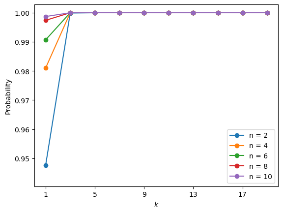
Figure 4: Probability of regularity condition with independently and uniformly distributed $x_{0}$ and $x^{*}$.

In Figure 4 we estimate the probability for the regularity condition for different $n$ and $k$ values with independently and uniformly distributed $x_{0}$ and $x^{*}$.

To sum up, in this section we have demonstrated how the closed form of the equilibrium allows us to easily analyze the effect of $\lambda$ on the welfare measures in the PNE. A similar analysis can be performed on the effect of the other game parameters.

Appendix C Learning Dynamics in the PRP Ranking Function

In this section, we delve into the learning dynamics of games induced by the PRP ranking function. While the dynamics in RRP-induced games are relatively easy to anticipate, as they converge to an $\varepsilon$-PNE in a few timesteps, PRP-based games often exhibit a completely different phenomenon. In this appendix, we will explore these intriguing dynamics in detail.

During the examination of the PRP ranking function, we noticed that the vast majority (about $99.5\%$) of the dynamics it induces belong to one of two types of dynamics. One type, which constitutes a minority of the cases, is when the simulation converges already in the first round because no publisher can improve her utility under the constraints of the discrete simulation. In those cases, the publisher whose initial document is farther from $x^{*}$ (the information need) cannot get closer to $x^{*}$ than the other publisher in a single step, and therefore cannot improve her utility in a single step. Moreover, the other publisher gets the maximum utility, $1$, because she is the closest to $x^{*}$ and she is at her initial document, therefore she also cannot improve her utility in a single step. In the other type of simulations, which constitutes most of the cases, the publishers enter a pseudo-periodic behavior that never converges. Figure 5 presents the welfare measures during one representative instance of the latter type of simulations.

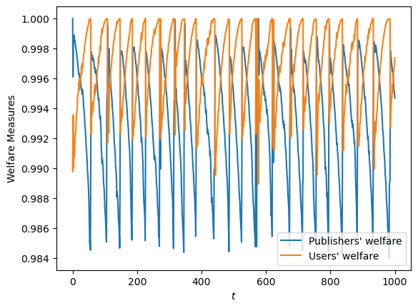
Figure 5: The welfare measures during a Discrete Better Response Dynamics Simulation with the PRP ranking function on a representative instance of a publishers’ game with $\lambda=0.5,n=2\text{ and }k=2$.

The periodic nature of the publishers’ behavior is evident in Figure 5. In each cycle, there is a period where the publishers compete to provide the closest document to $x^{*}$. Each of them repeatedly changes her document (strategy) by the smallest margin sufficient for her to get closer to the information need than her competitor. This competition, which is accompanied by an increase in the users’ welfare and a decrease in the publishers’ welfare, continues until one of the players resigns and abruptly returns as close as she can to her initial document. Her decision to resign is either because the discrete nature of the simulation prevents her from bypassing the other publisher or because further bypassing the other publisher is not beneficial for her since it positions her too far from her initial document. Immediately after this resignation, the publisher who won the competition takes a big step toward her initial document while still maintaining her position as the closest to $x^{*}$, since as long as she is still closer to $x^{*}$ than the other publisher, getting closer to her initial document is trivially beneficial for her. This mutual withdrawal is accompanied by a sharp decrease in users’ welfare and a sharp increase in publishers’ welfare. When the losing publisher notices the winning publisher’s retreat from $x^{*}$, she exploits the situation to get back to the competition and bypass her rival. The entire process is then repeated over and over.

It can be seen that the PRP reaches profiles with users’ welfare of almost 1, which is the optimal users’ welfare value, but it does not stay there. This explains why, despite the PRP being optimized for short-term relevance (i.e., for a fixed profile it maximizes the users’ welfare), its instability harms its long-term performance. This phenomenon once again emphasizes the need for the search for stability.

The periodicity is best observed when animating the documents in a two-dimensional embedding space, which can be done using the code provided with this paper. In this visualization, one can notice that during the simulation each publisher stays close to the line segment that connects $x^{*}$ with her initial document. This phenomenon is correlated with the theoretical result of Lemma 4, which determines that in games induced by the PRP ranking function or any RRP ranking function, any strategy that is outside this line segment is strictly dominated.

Appendix D The Effect of the Embedding Space Dimension

In this section, we discuss the effect of the embedding space dimension, $k$. This examination is more complicated than examining the effect of $\lambda$ since the time complexity of the simulation increases exponentially with $k$. We first discuss the effect of $k$ when using the RRP ranking functions we explored in Section 6 and then present two approaches to assess this effect when using the PRP ranking function, a direct approach and a dynamics-based approach. Finally, we discuss how the results of this section affect the comparison between the different ranking functions. Note that $k=1$ is essentially different than other $k$ values since it is the only case in which the possible movement directions in the Discrete Better Response Dynamics Simulation include all possible directions in the embedding space. This attribute, together with the fact that $k=1$ is not a realistic case regardless, leads us to omit it from our analysis.

D.1 Direct Examination of the Effect of $k$ on RRP Ranking Functions

We performed several simulations to directly test the effect of $k$ on the welfare measures and the convergence rate under the softmax RRP and the linear RRP ranking functions.

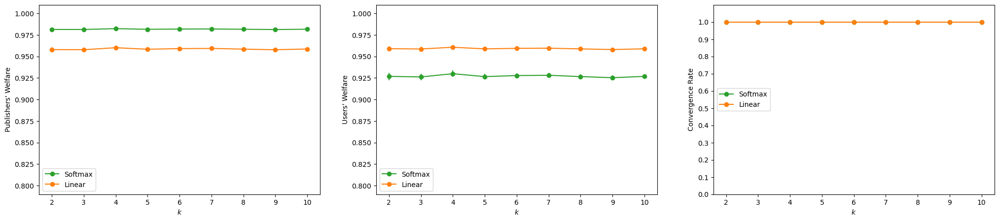
Figure 6: The effect of $k$ in the softmax RRP ($\beta=1$) and the linear RRP ($a=\frac{1}{n}=0.5$) ranking functions with $\lambda=0.5$ and $n=2$.

We can see that the convergence rates of both RRP ranking functions remain $1$ for all tested $k$ values. Furthermore, Figure 6 evidences that when using the softmax or the linear RRP ranking functions $k$ has a negligible effect on both the publishers’ and the users’ welfare. We observed similar results for other $\lambda$ values and different ranking functions hyperparameters. Therefore it can be said that the results in Section 6 regarding those functions can be extrapolated to any low-mid $k$ value. Examining high values of $k$ is highly impractical using this kind of simulation due to the exponential growth of the simulation running time as $k$ increases. However, note that all our theoretical results regarding the linear RRP ranking function hold for any $k$. In particular, the convergence of any $\varepsilon$-better response dynamics to a $\varepsilon$-PNE is guaranteed, and thus the convergence rate of the linear ranking function is guaranteed to be $1$ for any $k$. In the context of the softmax function, although we do not have any positive theoretical results regarding the convergence rate, we showed that since the game is smooth, there is always at least one PNE. Based on that, we conjecture that for all values of $k$, games induced by the softmax ranking function will have a convergence rate of $1$.

Furthermore, in Appendix A we presented Lemma 4, which determines that in games induced by any RRP ranking function, publishers should never play a strategy (document) that is not on the line segment that connects $x^{*}$ with their initial document. This result shows us that the nature of the dynamics in publishers’ games induced by any RRP ranking function is highly one-dimensional. That is, no matter how big $k$ is, each player still plays roughly on her one-dimensional line segment. This further strengthens our conjecture that the softmax ranking function will have a convergence rate of $1$ for all $k$. Furthermore, based on this argument, we can also conjecture that $k$ will have a negligible effect on the welfare measures of both the linear and softmax RRP ranking functions.

D.2 Direct Examination of the Effect of $k$ on the PRP Ranking Function

We now turn to discuss the effect of $k$ in PRP-induced publishers’ games, which introduces an increase in analytical complexity. In the Discrete Better Response Dynamics Simulation, the number of movement directions, and hence the simulation running time, grow exponentially with $k$. This challenge is further amplified when simulating the PRP ranking function, as the simulations frequently fail to converge. This makes simulations of the PRP ranking function with high values of $k$ highly impractical. Figure 7 presents the results for a few low values of $k$.

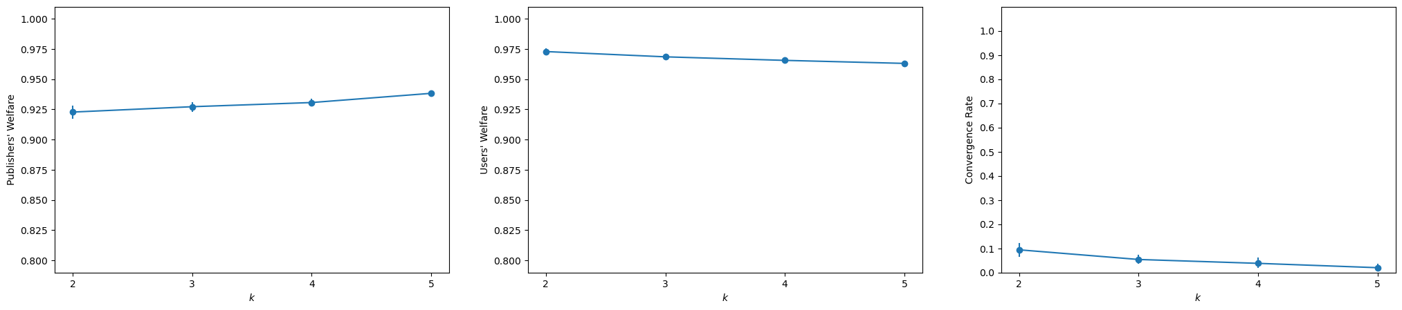
Figure 7: The effect of k in the PRP ranking function with $\lambda=0.5$ and $n=2$.

Figure 7 may indicate that as is the case for the RRP ranking functions, $k$ has a minor effect on the publishers’ and users’ welfare when using the PRP ranking function. We can see that as $k$ increases, the publishers’ welfare slightly increases and the users’ welfare slightly decreases. As mentioned, due to the structure of the simulation, we can’t examine the welfare measures with higher $k$ values, but we conjecture that the observed trends will continue until a certain limit.

Regarding the convergence rate, Figure 7 might suggest that it generally decreases with $k$ and that the decrease becomes more moderate as $k$ increases. As we only tested low values of $k$, it remains uncertain whether this trend holds for higher values of $k$. Therefore, we employ an alternative approach to approximate the effect of $k$ on the convergence rate of the PRP ranking function.

D.3 Dynamics-based Examination of the Effect of $k$ on the Convergence Rate of the PRP Ranking Function

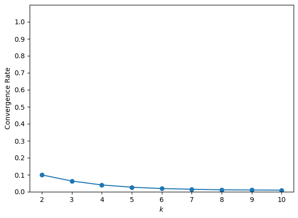
Figure 8: The effect of k on the PRP ranking function’s convergence rate with $\lambda=0.5$ and $n=2$.

In Appendix C we observed the two primary types of dynamics induced by the PRP ranking function, the uncommon type where the simulation converges already in the first timestep, and the common type where the publishers reach a pseudo-periodic behavior. Based on these results, we can use a new method to approximate the effect of $k$ on the convergence rate of the PRP ranking function. Instead of running a whole simulation each time, we can determine convergence at the beginning of the simulation. If the dynamics did not converge in the first timestep, we can deduce that the simulation will not converge. Figure 8 presents the convergence rate measured using this estimation method.

Figure 8 shows that the convergence rate of the PRP ranking function generally decreases as $k$ increases and that the decrease becomes more moderate as $k$ increases. In Appendix C, we saw that the only case when PRP dynamics converge is when the publisher whose initial document is farther from $x^{*}$ cannot bypass the other publisher in a single step. Therefore, a possible explanation for the decrease in the convergence rate is that a larger $k$ decreases the likelihood of this case. Although Figure 8 provides results only for $\lambda=0.5$, similar trends were observed for other values of $\lambda$. We conjecture that these trends will continue at higher $k$ values.

To conclude this section, let us revisit the trends we discovered in light of the results we have already seen in Section 6. From this perspective, we can see how an increase in $k$ emphasizes the consequences of the instability of the PRP ranking function. The already low convergence rate at $k=2$ further diminishes with increasing $k$, becoming very small. Simultaneously, the users’ welfare, a measure that the PRP is designed to maximize in the short term, also experiences a minor decline as $k$ increases. In contrast, the examination of different $k$ values underscores the stability of both the softmax and the linear RRP ranking functions, maintaining a convergence rate of $1$ and roughly identical welfare measures across all tested $k$ values.

Appendix E Proofs

E.1 Observation 1

Proof.

Assume by contradiction that $x^{eq}\in X$ is a PNE of $G$. By Lemma 7 we get that $\forall i\in N\;x^{eq}_{i}\in\{x^{*},x_{0}^{i}\}$. This means that there are only 4 profiles that can be PNEs of $G$. We proceed to show that none of them is a PNE.

• $x^{eq}=(x^{*},x_{0}^{2})$: player 1 can improve her utility by deviating to $\hat{x}_{1}=(\frac{1}{2},...,\frac{1}{2})$.

• $x^{eq}=(x_{0}^{1},x^{*})$: player 2 can improve her utility by deviating to $\hat{x}_{2}=(\frac{1}{2},...,\frac{1}{2})$.

• $x^{eq}=(x_{0}^{1},x_{0}^{2})$: player 1 can improve her utility by deviating to $\hat{x}_{1}=(\alpha,...,\alpha)$ for $0<\alpha<\sqrt{\frac{1}{2\lambda}}$ since $u_{1}(\hat{x}_{1},x^{eq}_{-1})=1-\lambda\alpha^{2}>1-\lambda\frac{1}{2\lambda}=\frac{1}{2}=u_{1}(x^{eq})$.

• $x^{eq}=(x^{*},x^{*})$: player 1 can improve her utility by deviating to $x_{0}^{1}$ since $u_{1}(x_{0}^{1},x^{eq}_{-1})=0-0>\frac{1}{2}-\lambda=u_{1}(x^{eq})$.

∎

Lemma 7.

Let $G$ be a publishers’ game with $r=r^{*}$ and $d(x,y)=\frac{1}{k}\left\lVert x-y\right\rVert_{2}^{2}$. If $x^{eq}$ is a PNE of $G$, then $x^{eq}_{i}\in\{x^{*},x_{0}^{i}\}\;\forall i\in N$.

Proof.

Assume by contradiction that there exists $i\in N$ such that $x^{eq}_{i}\notin\{x^{*},x_{0}^{i}\}$. By Lemma 4 we get that $x^{eq}_{i}\in L_{i}\coloneqq\{tx^{*}+(1-t)x_{0}^{i}:t\in[0,1]\}$. Thus $x_{0}^{i}\neq x^{*}$.
Recall the notation $\mu(x)\coloneqq\operatorname*{argmin}_{i\in N}{d^{*}(x_{i})}$ for $x\in X$. Let us divide the proof into the following cases:

1. If $i\notin\mu(x^{eq})$ then $u_{i}(x^{eq})=-\lambda d^{0}_{i}(x^{eq}_{i})$. Since $x^{eq}_{i}\neq x_{0}^{i}$ we get that $d^{0}_{i}(x^{eq}_{i})>0$ and hence $u_{i}(x^{eq})<0$. On the other hand, $u_{i}(x_{0}^{i},x^{eq}_{-i})=r_{i}(x_{0}^{i},x^{eq}_{-i})-0\geq 0$. Hence $u_{i}(x_{0}^{i},x^{eq}_{-i})>u_{i}(x^{eq})$ which is a contradiction to the fact that $x^{eq}$ is a PNE.

2. If $\mu(x^{eq})=\{i\}$ then $d^{*}(x^{eq}_{i})<d^{*}(x^{eq}_{j})\;\forall j\neq i$. Let us denote $\varepsilon=\frac{1}{2}\bigl{(}\min_{j\neq i}{d^{*}(x^{eq}_{j})}-d^{*}(x^{eq}_{i})\bigr{)}>0$. Since $d$ is continuous, $d^{*}$ is continuous and hence there exists a $\delta>0$ such that if $\left\lVert x_{i}-x^{eq}_{i}\right\rVert_{2}<\delta$ then $d^{*}(x_{i})<d^{*}(x^{eq}_{i})+\varepsilon$. Therefore, it holds in particular for

   $$\hat{x}_{i}\coloneqq x^{eq}_{i}+\frac{\delta}{2\left\lVert x^{eq}_{i}-x_{0}^{i}\right\rVert_{2}}(x_{0}^{i}-x^{eq}_{i})$$ (1)

   that $d^{*}(\hat{x}_{i})<d^{*}(x^{eq}_{i})+\varepsilon$ and hence $d^{*}(\hat{x}_{i})<\min_{j\neq i}{d^{*}(x^{eq}_{j})}$. Therefore $\mu(\hat{x}_{i},x^{eq}_{-i})=\{i\}$ and hence $r^{*}_{i}(\hat{x}_{i},x^{eq}_{-i})=1$. We get that:

   $$u_{i}(\hat{x}_{i},x^{eq}_{-i}) =1-\lambda d^{0}_{i}(\hat{x}_{i})=1-\lambda\frac{1}{k}\left\lVert\hat{x}_{i}-x_{0}^{i}\right\rVert_{2}^{2}=1-\lambda\frac{1}{k}\left\lVert(x^{eq}_{i}-x_{0}^{i})(1-\frac{\delta}{2\left\lVert x^{eq}_{i}-x_{0}^{i}\right\rVert_{2}})\right\rVert_{2}^{2}$$ (2)

   $$=1-\lambda\frac{1}{k}(1-\frac{\delta}{2\left\lVert x^{eq}_{i}-x_{0}^{i}\right\rVert_{2}})^{2}\left\lVert x^{eq}_{i}-x_{0}^{i}\right\rVert_{2}^{2}>1-\lambda\frac{1}{k}\left\lVert x^{eq}_{i}-x_{0}^{i}\right\rVert_{2}^{2}$$

   $$=1-\lambda d^{0}_{i}(x^{eq}_{i})=u_{i}(x^{eq})$$

   which is in contradiction to the fact that $x^{eq}$ is a PNE.

3. If $i\in\mu(x^{eq})$ and $|\mu(x^{eq})|\geq 2$:
   $d$ is continuous and hence $d^{0}_{i}$ is continuous. Therefore there exists a $\delta>0$ such that if $\left\lVert x_{i}-x^{eq}_{i}\right\rVert_{2}<\delta$ then $d^{0}_{i}(x_{i})<d^{0}_{i}(x^{eq}_{i})+\frac{1}{2\lambda}$. Therefore it holds in particular for

   $$\hat{x}_{i}\coloneqq x^{eq}_{i}+\frac{\delta}{2\left\lVert x^{eq}_{i}-x^{*}\right\rVert_{2}}(x^{*}-x^{eq}_{i})$$ (3)

   that $d^{0}_{i}(\hat{x}_{i})<d^{0}_{i}(x^{eq}_{i})+\frac{1}{2\lambda}$.

   Now, $d^{*}(\hat{x_{i}})=\frac{1}{k}\left\lVert\hat{x}_{i}-x^{*}\right\rVert_{2}^{2}=\frac{1}{k}\left\lVert(x^{eq}_{i}-x^{*})(1-\frac{\delta}{2\left\lVert x^{eq}_{i}-x^{*}\right\rVert_{2}})\right\rVert_{2}^{2}<\frac{1}{k}\left\lVert x^{eq}_{i}-x^{*}\right\rVert_{2}^{2}=d^{*}(x^{eq}_{i})$. Therefore $\mu(\hat{x}_{i},x^{eq}_{-i})=\{i\}$ and hence $r_{i}(\hat{x}_{i},x^{eq}_{-i})=1$. We get that:

   $$u_{i}(\hat{x}_{i},x^{eq}_{-i})=1-\lambda d^{0}_{i}(\hat{x}_{i})>1-\lambda\bigr{(}d^{0}_{i}(x^{eq}_{i})+\frac{1}{2\lambda}\bigl{)}=\frac{1}{2}-\lambda d^{0}_{i}(x^{eq}_{i})\geq\frac{1}{|\mu(x^{eq})|}-\lambda d^{0}_{i}(x^{eq}_{i})=u_{i}(x^{eq})$$ (4)

   which is once again a contradiction to the fact that $x^{eq}$ is a PNE.

∎

E.2 Theorem 2

Proof.

Assume by contradiction that there exists a proportional RRP ranking function $r$, defined by $r_{i}(x)=\frac{g\bigl{(}d^{*}(x_{i})\bigr{)}}{\sum_{j=1}^{n}g\bigl{(}d^{*}(x_{j})\bigr{)}}$, that induces a potential game. We show that the fact that $r$ induces a potential game implies that $g$ is constant. This is a contradiction to the requirement that $g$ must be strictly decreasing.

Since $r$ induces a potential game, any publishers’ game with $r$ as its ranking function is a potential game. In particular, any publishers’ game with $r$ as its ranking function, $k=1$ and $d$ twice continuously differentiable is a potential game. Such games, since $g>0$, satisfy the conditions of Theorem 4.5 in [MS96]. Therefore:

$$\frac{\partial^{2}u_{i}(x)}{\partial x_{i}\partial x_{j}}=\frac{\partial^{2}u_{j}(x)}{\partial x_{i}\partial x_{j}}\;\;\;\forall i,j\in[n],\forall x\in X$$ (5)

Recall $u_{i}(x)\coloneqq r_{i}(x)-\lambda d_{i}^{0}(x_{i})$. Since $\frac{\partial^{2}\lambda d_{i}^{0}(x_{i})}{\partial x_{i}\partial x_{j}}=\frac{\partial^{2}\lambda d_{j}^{0}(x_{i})}{\partial x_{i}\partial x_{j}}=0$, we get:

$$\frac{\partial^{2}r_{i}(x)}{\partial x_{i}\partial x_{j}}=\frac{\partial^{2}r_{j}(x)}{\partial x_{i}\partial x_{j}}\;\;\;\forall i,j\in[n],\forall x\in X$$ (6)

Note that $r_{i}$ can be written as:

$$r_{i}(x)=\frac{(g\circ d^{*})(x_{i})}{\sum\limits_{j=1}^{n}(g\circ d^{*})(x_{j})}$$ (7)

Hence, by Lemma 8 we see that $g\circ d^{*}$ is constant on $[0,1]$. And since this is true for every twice continuously differentiable $d^{*}$, it is true in particular for $x^{*}=0,d(a,b)=(a-b)^{2}$, which gives us $d^{*}(a)=a^{2}$. Note that in this case, the image of $d^{*}$ is precisely $[0,1]$. Therefore, $g$ is constant on $[0,1]$, which is a contradiction, since it should be strictly decreasing.

∎

Lemma 8.

Let $f:\mathbb{R}^{n}\to\mathbb{R}^{n}$ be of the form $f_{i}(x)=\frac{g(x_{i})}{\sum\limits_{j=1}^{n}g(x_{j})}$ for a continuously differentiable function $g:[0,1]\to\mathbb{R}$. Then

$$\frac{\partial^{2}f_{i}(x)}{\partial x_{i}\partial x_{j}}=\frac{\partial^{2}f_{j}(x)}{\partial x_{i}\partial x_{j}}\;\;\;\forall i,j\in[n],\forall x\in[0,1]^{n}$$ (8)

iff $g$ is constant on $[0,1]$.

Proof.

If $g$ is constant on $[0,1]$ then $f_{i}\equiv\frac{1}{n}\;\forall i\in[n]$ and then $f$ satisfies (8) trivially, since both sides of the equation are $0$.
In the other direction, assume that $f$ satisfies (8). Let us calculate the derivatives. It holds $\forall i,j\in[n]$ and $\forall x\in X$ that:

$$\frac{\partial f_{i}(x)}{\partial x_{j}}=\frac{-g(x_{i})g^{\prime}(x_{j})}{\left(\sum\limits_{k=1}^{n}g\left(x_{k}\right)\right)^{2}}$$ (9)

and

$$\frac{\partial^{2}f_{i}(x)}{\partial x_{i}\partial x_{j}}=\frac{g^{\prime}(x_{i})g^{\prime}(x_{j})\left(2g(x_{i})-\sum\limits_{k=1}^{n}g(x_{k})\right)}{\left(\sum\limits_{k=1}^{n}g(x_{k})\right)^{3}}$$ (10)

In the same way, we get:

$$\frac{\partial^{2}f_{j}(x)}{\partial x_{i}\partial x_{j}}=\frac{g^{\prime}(x_{i})g^{\prime}(x_{j})\left(2g(x_{j})-\sum\limits_{k=1}^{n}g(x_{k})\right)}{\left(\sum\limits_{k=1}^{n}g(x_{k})\right)^{3}}$$ (11)

So by (8) we get:

$$0=\frac{\partial^{2}f_{i}(x)}{\partial x_{i}\partial x_{j}}-\frac{\partial^{2}f_{j}(x)}{\partial x_{i}\partial x_{j}}=\frac{g^{\prime}(x_{i})g^{\prime}(x_{j})\left(2g(x_{i})-2g(x_{j})\right)}{\left(\sum\limits_{k=1}^{n}g(x_{k})\right)^{3}}$$ (12)

Hence, $\forall i,j\in[n]$ and $\forall x\in[0,1]^{n}$ it holds that:

$$g^{\prime}(x_{i})=0\;\vee\;g^{\prime}(x_{j})=0\;\vee\;g(x_{i})=g(x_{j})$$ (13)

Equivalently, (since $n\geq 2$):

$$g^{\prime}(a)=0\;\vee\;g^{\prime}(b)=0\;\vee\;g(a)=g(b)\;\;\;\forall a,b\in[0,1]$$ (14)

We proceed to show that (14) implies that $g$ is constant on $[0,1]$. We divide the proof into two cases:

• If there is no $a\in[0,1]$ such that $g^{\prime}(a)\neq 0$, then $g^{\prime}\equiv 0$ on $[0,1]$ and therefore $g$ is constant on $[0,1]$.

• Otherwise, let $a\in[0,1]$ be such that $g^{\prime}(a)\neq 0$. Without loss of generality, assume $g^{\prime}(a)>0$. By continuity of $g^{\prime}$, there is a $\delta>0$ such that $g^{\prime}(x)>0\;\forall x\in U:=(a-\delta,a+\delta)\cap[0,1]$. So $g$ is strictly increasing on $U$. Take $b\in U$. Since $g$ is strictly increasing on $U$, $g(a)\neq g(b)$. Also, $g^{\prime}(b)\neq 0$, $g^{\prime}(a)\neq 0$ since they are both positive. This is a contradiction to (14).

∎

E.3 Lemma 2

Proof.

Let $x\in X$ be an arbitrary strategy profile. First, notice that $-1\leq\nu_{i}(x)\leq 1$, and summing $\nu_{i}(x)$ over all publishers $i\in N$ yields:

$$\sum_{i=1}^{n}\nu_{i}(x)=\sum_{i=1}^{n}\Biggr{(}\frac{1}{n-1}\Bigr{(}\sum_{j\in N\setminus\{i\}}d^{*}(x_{j})\Bigl{)}-d^{*}(x_{i})\Biggl{)}=\frac{1}{n-1}\sum_{i=1}^{n}\Bigr{(}\sum_{j\in N\setminus\{i\}}d^{*}(x_{j})\Bigl{)}-\sum_{i=1}^{n}d^{*}(x_{i})$$ (15)

Note that for every $i\in N$, $d^{*}(x_{i})$ appears exactly $n-1$ in the left term and only one time in the right term. Therefore, the above sum equals zero. Now, let $\hat{r}^{a,b}$. To be a valid ranking function, $\hat{r}^{a,b}$ must satisfy the following conditions:

$$\sum_{i=1}^{n}\hat{r}^{a,b}_{i}(x)=1$$ (16)

$$\forall i\in N:0\leq\hat{r}^{a,b}_{i}(x)\leq 1$$ (17)

By definition, $\hat{r}^{a,b}(x)=a\nu_{i}(x)+b$. Therefore, from condition (16) combined with the fact that
$\sum_{i=1}^{n}\nu_{i}(x)=0$, we get:

$$1=\sum_{i=1}^{n}\hat{r}^{a,b}_{i}(x)=a\cdot\sum_{i=1}^{n}\nu_{i}(x)+n\cdot b=n\cdot b\Rightarrow b=\frac{1}{n}$$ (18)

Plugging into condition (17) and using the fact that $-1\leq\nu_{i}(x)\leq 1$, we get the following equivalent conditions:

$$0\leq-a+\frac{1}{n}\leq 1$$ (19)

$$0\leq a+\frac{1}{n}\leq 1$$ (20)

which can be compactly written as $-\frac{1}{n}\leq a\leq\frac{1}{n}$. Lastly, it is straightforward to show that the second condition of the RRP is satisfied if and only if $a>0$. Therefore, $\hat{r}^{a,b}$ is a valid probability distribution over $N$ and satisfies the RRP condition if and only if $0<a\leq\frac{1}{n}$ and $b=\frac{1}{n}$.

∎

E.4 Theorem 3

Proof.

Let $g(t)=at+\frac{1}{n}$, and notice that the linear ranking function can be now written as $\hat{r}_{i}(x)=g(\nu_{i}(x))$. We will show that the following function is a potential function for the game $G$:

$$\phi(x)=-\sum_{i=1}^{n}\bigr{(}-g(d^{*}(x_{i}))+\lambda d^{0}_{i}(x_{i})\bigl{)}$$ (21)

To show this, one should show that for any $i\in N,x_{-i}\in X_{-i},x^{\prime}_{i},x^{\prime\prime}_{i}\in X_{i}$:

$$\phi(x^{\prime}_{i},x_{-i})-\phi(x^{\prime\prime}_{i},x_{-i})=u_{i}(x^{\prime}_{i},x_{-i})-u_{i}(x^{\prime\prime}_{i},x_{-i})$$ (22)

Let $i\in N,x_{-i}\in X_{-i},x^{\prime}_{i},x^{\prime\prime}_{i}\in X_{i}$. Starting with the LHS, we get:

$$\phi(x^{\prime}_{i},x_{-i})-\phi(x^{\prime\prime}_{i},x_{-i})=$$ (23)

$$-g(d^{*}(x^{\prime}_{i}))-\lambda d^{0}_{i}(x^{\prime}_{i})+g(d^{*}(x^{\prime\prime}_{i}))+\lambda d^{0}_{i}(x^{\prime\prime}_{i})=$$

$$g(d^{*}(x^{\prime\prime}_{i})-d^{*}(x^{\prime}_{i}))+\lambda(d^{0}_{i}(x^{\prime\prime}_{i})-d^{0}_{i}(x^{\prime}_{i}))-\frac{1}{n}$$

On the other hand, simplifying the RHS yields:

$$u_{i}(x^{\prime}_{i},x_{-i})-u_{i}(x^{\prime\prime}_{i},x_{-i})=$$ (24)

$$g(\nu_{i}(x^{\prime}_{i},x_{-i}))-\lambda d^{0}_{i}(x^{\prime}_{i})-g(\nu_{i}(x^{\prime\prime}_{i},x_{-i}))+\lambda d^{0}_{i}(x^{\prime\prime}_{i})=$$

$$g(\nu_{i}(x^{\prime}_{i},x_{-i})-\nu_{i}(x^{\prime\prime}_{i},x_{-i}))+\lambda(d^{0}_{i}(x^{\prime\prime}_{i})-d^{0}_{i}(x^{\prime}_{i}))-\frac{1}{n}=$$

$$g(d^{*}(x^{\prime\prime}_{i})-d^{*}(x^{\prime}_{i}))+\lambda(d^{0}_{i}(x^{\prime\prime}_{i})-d^{0}_{i}(x^{\prime}_{i}))-\frac{1}{n}$$

The required equation (22) now follows directly from (23) and (24), which concludes the proof.

∎

E.5 Theorem 4

Fix some publisher $i$ and let us show she has a strictly dominant strategy. Player $i$’s utility is given by

$$u_{i}(x)=r_{i}(x)-\lambda d_{i}^{0}(x_{i})=\frac{\nu_{i}(x)}{n}+\frac{1}{n}-\lambda d_{i}^{0}(x_{i})=\Bigl{(}\sum\limits_{\begin{subarray}{c}j\in N\setminus\{i\}\end{subarray}}\frac{d^{*}(x_{j})}{n(n-1)}\Bigr{)}-\frac{d^{*}(x_{i})}{n}+\frac{1}{n}-\lambda d_{i}^{0}(x_{i})$$ (25)

Now, $\forall x_{-i}\in X_{-i}$:

$$\operatorname*{argmax}_{x_{i}\in X_{i}}\{u_{i}(x_{i},x_{-i})\} =\operatorname*{argmax}_{x_{i}\in X_{i}}\Bigl{\{}-\frac{d^{*}(x_{i})}{n}-\lambda d^{0}_{i}(x_{i})\Bigr{\}}$$ (26)

meaning that $\operatorname*{argmax}_{x_{i}\in X_{i}}\{u_{i}(x_{i},x_{-i})\}$ does not depend on $x_{-i}$. Note that since $g(x)=d(x,y)$ is strictly convex for any $y\in{[0,1]}^{k}$, we get in particular that $d^{0}_{i}$ and $d^{*}$ are strictly convex. This implies that $-\frac{d^{*}(x_{i})}{n}-\lambda d^{0}_{i}(x_{i})$ is strictly concave in $x_{i}$, and therefore has a unique maximizer. So we got that $\operatorname*{argmax}_{x_{i}\in X_{i}}\{u_{i}(x_{i},x_{-i})\}$ is a singleton that does not depend of $x_{-i}$.
Let us denote $\operatorname*{argmax}_{x_{i}\in X_{i}}\{u_{i}(x_{i},x_{-i})\}=\{x^{dom}_{i}\}$. Then, the strategy $x^{dom}_{i}$ is a strictly dominant strategy for player $i$ by definition.

We proved that each player has a strictly dominant strategy. Note that the strategy profile where each player plays her strictly dominant strategy is a PNE. The uniqueness of the PNE follows from the fact that a strictly dominated strategy can never be an equilibrium strategy, and each player has only one strategy that is not strictly dominated (her dominant strategy).

E.6 Lemma 3

Proof.

Let $G$ be a publishers’ game with $r=\hat{r}$ and $d(x,y)=\frac{1}{k}||x-y||^{2}_{2}$. From Theorem 3, a potential function for G is:

$$\hat{\phi}(x)=-\sum_{i=1}^{n}\biggr{(}\frac{d^{*}(x_{i})}{n}+\frac{1}{n}+\lambda d^{0}_{i}(x_{i})\biggl{)}=-\sum_{i=1}^{n}\biggr{(}\frac{||x_{i}-x^{*}||^{2}_{2}}{nk}+\frac{1}{n}+\lambda\frac{||x_{i}-x_{0}^{i}||^{2}_{2}}{k}\biggl{)}$$ (27)

We notice that $G$ is smooth and $\hat{\phi}$ is concave, therefore a strategy profile is a PNE if and only if it is a potential maximizer (see e.g. [Ney97]). In order to find a potential maximizer we will find stationary points by setting the gradient of the potential with respect to $x_{i}$ to $0_{k}$. We will denote those points by $x^{eq}$.

$$\nabla_{x_{i}}\hat{\phi}(x)=\frac{-2}{nk}(x_{i}-x^{*})-\frac{2\lambda}{k}(x_{i}-x_{0}^{i})$$ (28)

$$0_{k}=\nabla_{x_{i}}\hat{\phi}(x^{eq})\implies 0_{k}=-(x^{eq}_{i}-x^{*})-\lambda n(x^{eq}_{i}-x_{0}^{i})\implies 0_{k}=-\lambda nx^{eq}_{i}-x^{eq}_{i}+x^{*}+\lambda nx_{0}^{i}$$ (29)

$$\implies\forall i\in N,\;x^{eq}_{i}=\frac{x^{*}+\lambda nx_{0}^{i}}{1+\lambda n}$$ (30)

Since $\hat{\phi}$ is strictly concave, $x^{eq}$ is its unique maximizer and hence the only PNE in $G$. Note that the squared Euclidean norm is strictly biconvex (that is, $g(x)=\frac{1}{k}\left\lVert x-y\right\rVert^{2}_{2}$ is strictly convex for any $y\in{[0,1]}^{k}$). Therefore by Theorem 4, $x^{eq}_{i}$ is a strictly dominant strategy for every player $i$. ∎

E.7 Theorem 5

Proof.

Lemma 2 shows that all linear RRP ranking functions are RRP ranking functions. It remains to show that if a function $r$ of the form $r_{i}(x)=g\big{(}\nu_{i}(x)\big{)}$ for some $g:\operatorname*{\mathbb{R}}\to\operatorname*{\mathbb{R}}$ is an RRP ranking function, then $r$ is a linear RRP ranking function.

Let $r$ be of the form $r_{i}(x)=g\big{(}\nu_{i}(x)\big{)}$ for some $g:\operatorname*{\mathbb{R}}\to\operatorname*{\mathbb{R}}$ and suppose it is an RRP ranking function. From the differentiability requirement of the RRP, we get that $g$ must be differentiable. From Lemma 9 we get that the fact $r$ is a valid ranking function implies that $g$ is linear on $[-1,1]$, which suffices since $-1\leq\nu_{i}\leq 1$. From Lemma 2 we get that $g(t)=at+\frac{1}{n}$ for some $a\in(0,\frac{1}{n}]$, meaning $r$ is a linear RRP ranking function. This wraps up the proof. ∎

Lemma 9.

Let $g:[-1,1]\to\operatorname*{\mathbb{R}}$ differentiable and let $r:X\to\mathbb{R}^{n}$ defined as follows: $r_{i}(x)=g(\nu_{i}(x))$. If $r$ is a valid ranking function (meaning $Im(r)\subset\Delta^{n}$ for every publishers’ game), then $g$ is linear.

Proof.

If $r$ is a valid ranking function, then in particular its image is contained in the simplex $\Delta^{n}$ for every publishers’ game with $n=3,k=1,x^{*}=0,d(a,b)=(a-b)^{2}$. Thus for every such game, $\forall x\in X=[0,1]^{3}$ it holds that:

$$1=\sum_{j=1}^{n}r_{j}(x)=\sum_{j=1}^{n}g(\nu_{j}(x))$$ (31)

Define a function $f:X\to\mathbb{R}$ by $f(x)=\sum\limits_{j=1}^{3}g(\nu_{j}(x))$. Since $f\equiv 1$ on $X$, $\nabla f(x)=\begin{pmatrix}0\\ 0\\ 0\\ \end{pmatrix}$ for all $x\in X$. Note that in such games, $d^{*}(a)=(a-0)^{2}=a^{2}$ and thus ${d^{*}}^{\prime}(a)=2a$. So $\forall x\in X,\forall i\in[n]$ it holds:

$$0=\frac{\partial f(x)}{\partial x_{i}}=\sum_{j\neq i}g^{\prime}\big{(}\nu_{j}(x)\big{)}\cdot\frac{2x_{i}}{n-1}-g^{\prime}\big{(}\nu_{i}(x)\big{)}\cdot 2x_{i}$$ (32)

Denote by $\psi:\mathbb{R}^{n}\to\mathbb{R}^{n}$ the function defined by

$$\psi_{i}(d)\coloneqq\frac{1}{n-1}\sum\limits_{j\neq i}d_{j}-d_{i}$$ (33)

By (32), $\forall i\in N$:

$$0=2x_{i}\cdot\psi_{i}\biggl{(}\Bigl{(}g^{\prime}\bigl{(}\nu_{l}(x)\bigr{)}\Bigr{)}_{l=1}^{n}\biggr{)}$$ (34)

Where $\Bigl{(}g^{\prime}\bigl{(}\nu_{l}(x)\bigr{)}\Bigr{)}_{l=1}^{n}$ stands for the vector $\begin{pmatrix}g^{\prime}\bigl{(}\nu_{1}(x)\bigr{)}&g^{\prime}\bigl{(}\nu_{2}(x)\bigr{)}&\dots&g^{\prime}\bigl{(}\nu_{n}(x)\bigr{)}\end{pmatrix}\in\operatorname*{\mathbb{R}}^{n}$.

Hence $\forall x\in X,\forall i,j\in[n]$ the following holds:

$$x_{i}\neq 0\land x_{j}\neq 0\implies\psi_{i}\biggl{(}\bigl{(}g^{\prime}\left(\nu_{l}(x)\right)\bigr{)}_{l=1}^{n}\biggr{)}=0=\psi_{j}\biggl{(}\bigl{(}g^{\prime}\left(\nu_{l}(x)\right)\bigr{)}_{l=1}^{n}\biggr{)}$$ (35)

Thus by Lemma 10, $\forall x\in X,\forall i,j\in[n]$ it holds that:

$$x_{i}\neq 0\land x_{j}\neq 0\implies g^{\prime}\left(v_{i}(x)\right)=g^{\prime}\left(v_{j}(x)\right)$$ (36)

Now, we prove that $g$ must be linear by proving that $g^{\prime}$ must be constant on $[-1,1]$. We do this in two steps: first, we show that $g^{\prime}$ is constant on $(-0.75,0.75)$ and then we show it is constant on the entire $[-1,1]$ as well.

For the first step, we look at the profiles $x_{\varepsilon}:=\left(\sqrt{0.5-\varepsilon},\sqrt{0.5},\sqrt{0.5+\varepsilon}\right)$ for $\varepsilon\in(0,0.5)$. The linear relative relevance vector in this case is $\nu(x_{\varepsilon})=(1.5\varepsilon,0,-1.5\varepsilon)$
By applying (36) on $x_{\varepsilon},i=1,j=2$ we get $g^{\prime}(1.5\varepsilon)=g^{\prime}(0)$.
And by applying (36) on $x_{\varepsilon},i=2,j=3$ we get $g^{\prime}(-1.5\varepsilon)=g^{\prime}(0)$.
So we got $\forall\varepsilon\in(0,0.5),g^{\prime}(-1.5\varepsilon)=g^{\prime}(0)=g^{\prime}(1.5\varepsilon)$.
This means that $\forall t\in(0,0.75),g^{\prime}(-t)=g^{\prime}(0)=g^{\prime}(t)$.
So $g^{\prime}$ is constant on $(-0.75,0.75)$.

Now for the second step, let $t\in(-1,1)$ and we show that $g^{\prime}(t)=g^{\prime}(0)$. Look at the profile $\hat{x}:=\left(\sqrt{\frac{1-t}{2}},\sqrt{\frac{1+t}{2}},\sqrt{\frac{1+t}{2}}\right)$. The linear relative relevance vector in this case is $v(\hat{x})=\left(t,-\frac{t}{2},-\frac{t}{2}\right)$.
By applying (36) on $\hat{x},i=1,j=2$ we get $g^{\prime}(t)=g^{\prime}\left(-\frac{t}{2}\right)$. Since $t\in(0,1)$, $-\frac{t}{2}\in(-0.75,0.75)$, so by the first step we have that $g^{\prime}\left(-\frac{t}{2}\right)=g(0)$. So $g^{\prime}(t)=g^{\prime}(0)$ as we wanted to show. This proves that $g^{\prime}$ is constant on $(-1,1)$. Therefore, $g$ is linear on $(-1,1)$. Since $g$ is continuous, it is also linear on $[-1,1]$.

∎

Lemma 10.

Let $\psi:\mathbb{R}^{n}\to\mathbb{R}^{n}$ the function defined by $\psi_{i}(d)=\frac{1}{n-1}\sum\limits_{j\neq i}d_{j}-d_{i}$. Then $\forall d\in\mathbb{R}^{n},\forall i,j\in[n]$,

$$\psi_{i}(d)=\psi_{j}(d)\iff d_{i}=d_{j}$$ (37)

Proof.

$$\psi_{i}(d)=\frac{1}{n-1}\sum\limits_{j\neq i}d_{j}-d_{i}=\frac{1}{n-1}\sum\limits_{j=1}^{n}d_{j}-\frac{n}{n-1}d_{i}$$ (38)

So

$$\psi_{i}(d)=\psi_{j}(d)\iff\frac{n}{n-1}d_{i}=\frac{n}{n-1}d_{j}\iff d_{i}=d_{j}$$ (39)

∎

E.8 Lemma 4

Proof.

We use the fact that since $L_{i}$ is convex and closed, $P_{L_{i}}(x_{i})$ is well defined and unique, and the following holds [BHM99]:

$$\forall y\in L_{i},\left\langle x_{i}-P_{L_{i}}(x_{i}),y-P_{L_{i}}(x_{i})\right\rangle\leq 0$$ (40)

where $\langle\cdot,\cdot\rangle$ stands for the standard inner product.

Also, if $x_{i}\notin L_{i}$, then $P_{L_{i}}(x_{i})\neq x_{i}$ so $\left\lVert x_{i}-P_{L_{i}}(x_{i})\right\rVert>0$. We get that for every $y\in L_{i}$:

$$\left\lVert x_{i}-y\right\rVert^{2} =\left\lVert x_{i}-P_{L_{i}}(x_{i})+P_{L_{i}}(x_{i})-y\right\rVert^{2}$$ (41)

$$=\left\lVert x_{i}-P_{L_{i}}(x_{i})\right\rVert^{2}+\left\lVert P_{L_{i}}(x_{i})-y\right\rVert^{2}+2\left\langle x_{i}-P_{L_{i}}(x_{i}),P_{L_{i}}(x_{i})-y\right\rangle$$

$$\underset{\eqref{eq:projection}}{\geq}\left\lVert x_{i}-P_{L_{i}}(x_{i})\right\rVert^{2}+\left\lVert P_{L_{i}}(x_{i})-y\right\rVert^{2}>\left\lVert P_{L_{i}}(x_{i})-y\right\rVert^{2}$$

Hence in particular $\left\lVert x_{i}-x^{*}\right\rVert>\left\lVert P_{L_{i}}(x_{i})-x^{*}\right\rVert$, and thus $d^{*}(x_{i})>d^{*}\left(P_{L_{i}}(x_{i})\right)$, so either $r$ is an RRP ranking function, in which case by the RRP principle $r_{i}(x_{i},x_{-i})<r_{i}(P_{L_{i}}(x_{i}),x_{-i})\;\forall x_{-i}\in X_{-i}$; or $r$ is the PRP ranking function, in which case $r_{i}(x_{i},x_{-i})\leq r_{i}(P_{L_{i}}(x_{i}),x_{-i})\;\forall x_{-i}\in X_{-i}$.
In the same way, $\left\lVert x_{i}-x_{i}^{0}\right\rVert>\left\lVert P_{L_{i}}(x_{i})-x_{i}^{0}\right\rVert$, so $d^{0}_{i}(x_{i})>d^{0}_{i}\left(P_{L_{i}}(x_{i})\right)$. By combining these two inequalities we get that

$$u_{i}(x_{i},x_{-i})=r_{i}(x_{i},x_{-i})-\lambda d^{0}_{i}(x_{i})<r_{i}(P_{L_{i}}(x_{i}),x_{-i})-\lambda d^{0}_{i}\left(P_{L_{i}}(x_{i})\right)=u_{i}\left(P_{L_{i}}(x_{i}),x_{-i}\right)\;\;\;\forall x_{-i}\in X_{-i}$$ (42)

so $x_{i}$ is strictly dominated by $P_{L_{i}}(x_{i})$ in $G$. ∎

E.9 Lemma 5

Proof.

Let G be a publishers’ game with $d(x,y)=\frac{1}{\sqrt{k}}||x-y||_{2}$, and let $i\in N,\;x_{i}\in L_{i}$. By definition, $\exists t\in[0,1]$ s.t. $x_{i}=tx^{*}+(1-t)x_{0}^{i}$.

$$d(x_{0}^{i},x^{*}) =\frac{||x_{0}^{i}-x^{*}||_{2}}{\sqrt{k}}=t\cdot\frac{||x^{*}-x_{0}^{i}||_{2}}{\sqrt{k}}+(1-t)\cdot\frac{||x_{0}^{i}-x^{*}||_{2}}{\sqrt{k}}$$ (43)

$$=\frac{||tx^{*}-tx_{0}^{i}+x_{0}^{i}-x_{0}^{i}||_{2}}{\sqrt{k}}+\frac{||(1-t)x_{0}^{i}-(1-t)x^{*}||_{2}}{\sqrt{k}}$$

$$=\frac{||tx^{*}+(1-t)x_{0}^{i}-x_{0}^{i}||_{2}}{\sqrt{k}}+\frac{||tx^{*}+(1-t)x_{0}^{i}-x^{*}||_{2}}{\sqrt{k}}$$

$$=\frac{||x_{i}-x_{0}^{i}||_{2}}{\sqrt{k}}+\frac{||x_{i}-x^{*}||_{2}}{\sqrt{k}}=d^{0}_{i}(x_{i})+d^{*}(x_{i})$$

∎

E.10 Lemma 6

Proof.

Let G be a publishers’ game with $r=\hat{r}$ and $d(x,y)=\frac{||x-y||_{2}}{\sqrt{k}}$. First, we notice that:

$$u_{i}(x) =r_{i}(x)-\lambda d_{i}^{0}(x_{i})=\frac{\nu_{i}(x)}{n}+\frac{1}{n}-\lambda d_{i}^{0}(x_{i})=\bigl{(}\sum\limits_{\begin{subarray}{c}j\in N\setminus\{i\}\end{subarray}}\frac{d^{*}(x_{j})}{n(n-1)}\bigr{)}-\frac{d^{*}(x_{i})}{n}+\frac{1}{n}-\lambda d_{i}^{0}(x_{i})$$ (44)

Now, for every player $i\in N$ and $\forall x_{-i}\in X_{-i}$:

$$\operatorname*{argmax}_{x_{i}\in X_{i}}\{u_{i}(x_{i},x_{-i})\} \overset{(1)}{{=}}\operatorname*{argmax}_{x_{i}\in L_{i}}\{u_{i}(x_{i},x_{-i})\}\overset{(2)}{{=}}\operatorname*{argmax}_{x_{i}\in L_{i}}\Bigl{\{}-\frac{d^{*}(x_{i})}{n}-\lambda d_{0}(x_{i})\Bigr{\}}$$ (45)

$$=\operatorname*{argmin}_{x_{i}\in L_{i}}\Bigl{\{}d^{*}(x_{i})+\lambda nd_{0}(x_{i})\Bigr{\}}\overset{(3)}{{=}}\operatorname*{argmin}_{x_{i}\in L_{i}}\Bigl{\{}d(x_{0}^{i},x^{*})-d_{i}^{0}(x_{i})+\lambda nd_{0}(x_{i})\Bigr{\}}$$

$$=\operatorname*{argmin}_{x_{i}\in L_{i}}\Bigl{\{}(\lambda n-1)d_{i}^{0}(x_{i})\Bigr{\}}=\begin{cases}\{x^{*}\},\text{ if }\lambda n<1\\ L_{i},\text{ if }\lambda n=1\\ \{x_{0}^{i}\},\text{ if }\lambda n>1\end{cases}$$

When transition $(1)$ is based on Lemma 4, transition $(2)$ is substitution and removal of terms that do not depend on $x_{i}$ and transition $(3)$ is based on Lemma 5. This wraps up the proof, since a profile $x$ is a PNE if and only if for every player $i\in N$ it holds that $x_{i}\in\operatorname*{argmax}\limits_{x^{\prime}_{i}\in X_{i}}\{u_{i}(x^{\prime}_{i},x_{-i})\}$.

∎

References

- [ABV21] Mohsen Abbasi, Aditya Bhaskara, and Suresh Venkatasubramanian. Fair clustering via equitable group representations. In Proceedings of the 2021 ACM conference on fairness, accountability, and transparency, pages 504–514, 2021.
- [BBPLBT20] Gal Bahar, Omer Ben-Porat, Kevin Leyton-Brown, and Moshe Tennenholtz. Fiduciary bandits. In International Conference on Machine Learning, pages 518–527. PMLR, 2020.
- [BBTK15] Ran Ben Basat, Moshe Tennenholtz, and Oren Kurland. The probability ranking principle is not optimal in adversarial retrieval settings. In Proceedings of the 2015 International Conference on The Theory of Information Retrieval, pages 51–60, 2015.
- [BHM99] Dimitri P Bertsekas, W Hager, and O Mangasarian. Nonlinear programming. athena scientific belmont. Massachusets, USA, 1999.
- [BPGRT19] Omer Ben-Porat, Gregory Goren, Itay Rosenberg, and Moshe Tennenholtz. From recommendation systems to facility location games. In Proceedings of the AAAI Conference on Artificial Intelligence, volume 33, pages 1772–1779, 2019.
- [BPRT19] Omer Ben-Porat, Itay Rosenberg, and Moshe Tennenholtz. Convergence of learning dynamics in information retrieval games. In Proceedings of the AAAI Conference on Artificial Intelligence, volume 33, pages 1780–1787, 2019.
- [BPST21] Omer Ben-Porat, Fedor Sandomirskiy, and Moshe Tennenholtz. Protecting the protected group: Circumventing harmful fairness. In Proceedings of the AAAI Conference on Artificial Intelligence, volume 35, pages 5176–5184, 2021.
- [BPT18] Omer Ben-Porat and Moshe Tennenholtz. A game-theoretic approach to recommendation systems with strategic content providers. Advances in Neural Information Processing Systems, 31, 2018.
- [BSKC13] Olga Butman, Anna Shtok, Oren Kurland, and David Carmel. Query-performance prediction using minimal relevance feedback. In Proceedings of the 2013 Conference on the Theory of Information Retrieval, pages 14–21, 2013.
- [BTK17] Ran Ben Basat, Moshe Tennenholtz, and Oren Kurland. A game theoretic analysis of the adversarial retrieval setting. Journal of Artificial Intelligence Research, 60:1127–1164, 2017.
- [CB98] Caroline Claus and Craig Boutilier. The dynamics of reinforcement learning in cooperative multiagent systems. AAAI/IAAI, 1998(746-752):2, 1998.
- [CDE+14] Matthew Cary, Aparna Das, Benjamin Edelman, Ioannis Giotis, Kurtis Heimerl, Anna R Karlin, Scott Duke Kominers, Claire Mathieu, and Michael Schwarz. Convergence of position auctions under myopic best-response dynamics. ACM Transactions on Economics and Computation (TEAC), 2(3):1–20, 2014.
- [CKLV17] Flavio Chierichetti, Ravi Kumar, Silvio Lattanzi, and Sergei Vassilvitskii. Fair clustering through fairlets. Advances in neural information processing systems, 30, 2017.
- [FS99] Yoav Freund and Robert E Schapire. Adaptive game playing using multiplicative weights. Games and Economic Behavior, 29(1-2):79–103, 1999.
- [HMPW16] Moritz Hardt, Nimrod Megiddo, Christos Papadimitriou, and Mary Wootters. Strategic classification. In Proceedings of the 2016 ACM conference on innovations in theoretical computer science, pages 111–122, 2016.
- [JGP+17] Thorsten Joachims, Laura Granka, Bing Pan, Helene Hembrooke, and Geri Gay. Accurately interpreting clickthrough data as implicit feedback. In Acm Sigir Forum, volume 51, pages 4–11. Acm New York, NY, USA, 2017.
- [KT22] Oren Kurland and Moshe Tennenholtz. Competitive search. In Proceedings of the 45th International ACM SIGIR Conference on Research and Development in Information Retrieval, pages 2838–2849, 2022.
- [LR22] Sagi Levanon and Nir Rosenfeld. Generalized strategic classification and the case of aligned incentives. In International Conference on Machine Learning, pages 12593–12618. PMLR, 2022.
- [LW16] Chang Liu and Yiming Wei. The impacts of time constraint on users’ search strategy during search process. Proceedings of the Association for Information Science and Technology, 53(1):1–9, 2016.
- [MCBP+20] Martin Mladenov, Elliot Creager, Omer Ben-Porat, Kevin Swersky, Richard Zemel, and Craig Boutilier. Optimizing long-term social welfare in recommender systems: A constrained matching approach. In International Conference on Machine Learning, pages 6987–6998. PMLR, 2020.
- [Mil96] Igal Milchtaich. Congestion games with player-specific payoff functions. Games and economic behavior, 13(1):111–124, 1996.
- [MPRJ10] Reshef Meir, Maria Polukarov, Jeffrey Rosenschein, and Nicholas Jennings. Convergence to equilibria in plurality voting. In Proceedings of the AAAI conference on artificial intelligence, volume 24, pages 823–828, 2010.
- [MS96] Dov Monderer and Lloyd S Shapley. Potential games. Games and economic behavior, 14(1):124–143, 1996.
- [Nag98] Anna Nagurney. Network economics: A variational inequality approach, volume 10. Springer Science & Business Media, 1998.
- [Ney97] Abraham Neyman. Correlated equilibrium and potential games. International Journal of Game Theory, 26:223–227, 1997.
- [NGTCR22] Vineet Nair, Ganesh Ghalme, Inbal Talgam-Cohen, and Nir Rosenfeld. Strategic representation. In International Conference on Machine Learning, pages 16331–16352. PMLR, 2022.
- [NST18] Kobbi Nissim, Rann Smorodinsky, and Moshe Tennenholtz. Segmentation, incentives, and privacy. Mathematics of Operations Research, 43(4):1252–1268, 2018.
- [QXLL19] Yifan Qiao, Chenyan Xiong, Zhenghao Liu, and Zhiyuan Liu. Understanding the behaviors of bert in ranking. arXiv preprint arXiv:1904.07531, 2019.
- [Rob77] Stephen E Robertson. The probability ranking principle in ir. Journal of documentation, 1977.
- [Ros73] Robert W Rosenthal. A class of games possessing pure-strategy nash equilibria. International Journal of Game Theory, 2:65–67, 1973.
- [RRTK17] Nimrod Raifer, Fiana Raiber, Moshe Tennenholtz, and Oren Kurland. Information retrieval meets game theory: The ranking competition between documents’ authors. In Proceedings of the 40th International ACM SIGIR Conference on Research and Development in Information Retrieval, pages 465–474, 2017.
- [YNL21] Andrew Yates, Rodrigo Nogueira, and Jimmy Lin. Pretrained transformers for text ranking: Bert and beyond. In Proceedings of the 14th ACM International Conference on web search and data mining, pages 1154–1156, 2021.
- [ZLRW22] Wayne Xin Zhao, Jing Liu, Ruiyang Ren, and Ji-Rong Wen. Dense text retrieval based on pretrained language models: A survey. arXiv preprint arXiv:2211.14876, 2022.
- [ZML+20] Jingtao Zhan, Jiaxin Mao, Yiqun Liu, Min Zhang, and Shaoping Ma. Learning to retrieve: How to train a dense retrieval model effectively and efficiently. arXiv preprint arXiv:2010.10469, 2020.