Fractional model of COVID–19 with pathogens as shedding effects

Abstract

To develop effective strategies for controlling the spread of the virus and potential future outbreaks, a deep understanding of disease transmission dynamics is crucial. This study proposes a modification to existing mathematical models used to describe the transmission dynamics of COVID-19 with environmental pathogens, incorporating a variable population, and employing incommensurate fractional order derivatives in ordinary differential equations. Our analysis accurately computes the basic reproduction number and demonstrates the global stability of the disease-free equilibrium point. Numerical simulations fitted to real data from South Africa show the efficacy of our proposed model, with fractional models enhancing flexibility. We also provide reliable values for initial conditions, model parameters, and order derivatives, and examine the sensitivity of model parameters. Our study provides valuable insights into COVID-19 transmission dynamics and has the potential to inform the development of effective control measures and prevention strategies.

1 Introduction

The COVID-19 pandemic has had severe consequences on global public health. To contain the spread of COVID-19 and prevent future viral outbreaks, a comprehensive understanding of the disease transmission dynamics is essential. Several mathematical models have been developed to describe the spread of the virus, including the traditional SIR and SEIR models. In this context, various incidence functions exist to model virus mutations during infection when the dynamics of infectious individuals undergo changes. Examples include the bilinear incidence or law of mass action described in [1] and [2], the saturated incidence function in [3] and [4], and the Beddington–DeAngelis function in [5] and [6]. Other specific nonlinear incidence functions are also used in [7] and [8], and recent developments in this field suggest utilizing Stieltjes derivatives to model time-varying contact rates and other parameters [9].

Although various mathematical models have been developed to describe the transmission of epidemic diseases, their efficacy is limited due to their assumption of uniform mixing of individuals, thereby failing to account for the complex dynamics of the disease, including the transmission of live viruses through contaminated environments. Recent research has attempted to overcome the limitations of traditional models by proposing interventions that account for environmental pathogens [10, 11, 12]. However, while these models have shown promise, there have been challenges in fitting real-world data due to the stringent mathematical conditions required for having positive and bounded solutions [10]. These conditions can sometimes conflict with biologically feasible regions, leading to difficulties in accurately representing the complex dynamics of the disease. To address this issue, our study proposes a modification to the existing model by incorporating a variable population and birth rate, which enables us to better capture the complex and evolving nature of disease spread.

Fractional calculus has been identified as a promising approach to improving the efficiency of disease transmission models [13, 14, 15, 16]. By incorporating memory and long-range dependence into the models, fractional calculus offers greater flexibility in capturing the complex and heterogeneous nature of disease dynamics, including demographics, social behaviors, and interventions that affect transmission dynamics.

While previous studies have utilized fractional order derivatives for modeling disease transmission and taking into account environment and social distancing [13], issues with mathematical rigor and accuracy of critical values, such as the basic reproduction number ($R_{0}$), have been identified. In our study, we address these issues by providing accurate computation of $R_{0}$ and demonstrating the global stability of the disease-free equilibrium point. Additionally, we employ incommensurate fractional order derivatives in ordinary differential equations (ODEs) to refine the description of memory effects and improve the model’s accuracy in capturing the impact of past infections on future transmissions.

The article is structured as follows. Section 2 presents the model structure, which incorporates Caputo fractional derivatives and multiple classes of individuals, including susceptible, exposed, symptomatic, and asymptomatic infectious, recovery, and environmental pathogen compartments, with corresponding coefficients. In Section 3, the mathematical analysis of the model is provided, including the derivation of the basic reproduction number and the study of the disease-free equilibrium. Section 4 presents the numerical findings, including the fitting of the model to real data from South Africa. Additionally, sensitivity analysis is performed to evaluate the effect of various model parameters on the basic reproduction number, which offers valuable insights for designing effective measures to contain the spread of COVID-19.

2 The fractional-order model

In this section, we introduce a modified fractional compartmental model of COVID-19 formerly proposed by [10] as follows:

$$\begin{cases}\displaystyle{{}^{C}D^{\alpha_{S}}_{0+}S(t)=\Lambda N(t)-\frac{\beta_{1}S(t)W(t)}{1+\phi_{1}W(t)}-\frac{\beta_{2}S(t)\left(I_{A}(t)+I_{S}(t)\right)}{1+\phi_{2}\left(I_{A}(t)+I_{S}(t)\right)}+\psi E(t)-\mu S(t)},\\[8.53581pt] \displaystyle{{}^{C}D^{\alpha_{E}}_{0+}E(t)=\frac{\beta_{1}S(t)W(t)}{1+\phi_{1}W(t)}+\frac{\beta_{2}S(t)\left(I_{A}(t)+I_{S}(t)\right)}{1+\phi_{2}\left(I_{A}(t)+I_{S}(t)\right)}-\psi E(t)-\mu E(t)-\omega E(t)},\\[8.53581pt] \displaystyle{{}^{C}D^{\alpha_{I_{A}}}_{0+}I_{A}(t)=(1-\delta)\omega E(t)-(\mu+\sigma)I_{A}(t)-\gamma_{A}I_{A}(t)},\\[8.53581pt] \displaystyle{{}^{C}D^{\alpha_{I_{S}}}_{0+}I_{S}(t)=\delta\omega E(t)-(\mu+\sigma)I_{S}(t)-\gamma_{S}I_{S}(t)},\\[8.53581pt] \displaystyle{{}^{C}D^{\alpha_{R}}_{0+}R(t)=\gamma_{S}I_{S}(t)+\gamma_{A}I_{A}(t)-\mu R(t)},\\[8.53581pt] \displaystyle{{}^{C}D^{\alpha_{W}}_{0+}W(t)=\eta_{A}I_{A}(t)+\eta_{S}I_{S}(t)-\mu_{P}W(t)}.\end{cases}$$ (1)

The model consists of six mutually exclusive compartments, that can be described as follows: Susceptible individuals denoted by $S$, Exposed individuals by $E$, Asymptomatic infectious individuals by $I_{A}$, Symptomatic infectious individuals by $I_{S}$, and Recovered individuals by $R$ with a separate class of compartment for pathogens in the environment denoted by $W$. The description of the model parameters is presented in Table 1.

Table 1: Description of the parameters.

parameter	description
$\Lambda$	birth rate in the population
$\mu$	natural human death rate
$\mu_{P}$	death rate of pathogens viruses
$\phi_{1}$	proportion of interaction with an infectious environment
$\phi_{2}$	proportion of interaction with an infectious individual
$\beta_{1}$	infection rate from $S$ to $E$ due to contact with W
$\beta_{2}$	infection rate from $S$ to $E$ due to contact with $I_{A}$ and/or $I_{S}$
$\delta$	proportion of symptomatic infectious people
$\psi$	progression rate from $E$ back to $S$ due to robust immune system
$\omega$	progression rate from $E$ to either $I_{A}$ or $I_{S}$
$\sigma$	disease mortality rate
$\gamma_{S}$	rate of recovery of the symptomatic individuals
$\gamma_{A}$	rate of recovery of the asymptomatic individuals
$\eta_{S}$	rate of virus spread to environment by $I_{S}$
$\eta_{A}$	rate of virus spread to environment by $I_{A}$

The fractional-order dynamics of the involved population denoted by $N$, can be obtained by summing the first five equations of model (1), given by

$${{}^{C}D^{\alpha_{N}}_{0+}N(t)=\Lambda N(t)-\sigma\left(I_{A}(t)+I_{S}(t)\right)-\mu N(t).}$$ (2)

Hence, we present a novel approach to modeling by incorporating a coupling equation (2) into (1), particularly its first equation involving $\Lambda N(t)$. This coupling equation allows us to account for population density in the recruitment rate of susceptible individuals. This approach differs from that of [10], which did not incorporate a similar coupling equation.

The transmission of viruses between healthy and non-healthy individuals is determined by the forces of infection $\displaystyle{\frac{\beta_{1}SW}{1+\phi_{1}W},\;\frac{\beta_{2}S(I_{A}+I_{S})}{1+\phi_{2}(I_{A}+I_{S})}}$, which are indicative of saturation in the incidence functions [17, 18, 19, 20]. According to [10], the selection of these forces of infection is based on their ability to account for contact minimization with infectious individuals through social distancing. Furthermore, [21] incorporates this saturated function response into the COVID-19 system dynamics to capture behavioral changes and the crowding effect of the population. Given these considerations, it appears that the authors of these works have focused on incorporating relevant biological and behavioral factors into their models.

3 Basic reproduction number and stability analysis

The basic reproduction number is computed using the method of the next-generation matrix [22] associated with our model (1). In doing so, the rate of appearance of new infection in the infectious compartment (that is $\mathcal{X}=(E,I_{A},I_{S},W$)), is given by

$$\mathcal{F(X)}=\begin{pmatrix}\frac{\beta_{1}S(t)W(t)}{1+\phi_{1}W(t)}+\frac{\beta_{2}S(t)\left(I_{A}(t)+I_{S}(t)\right)}{1+\phi_{2}\left(I_{A}(t)+I_{S}(t)\right)}\\ 0\\ 0\\ 0\end{pmatrix},$$

and the rate of other transitions involving shedding compartment is obtained as follows

$$\mathcal{V(X)}=\begin{pmatrix}(\psi+\mu+\omega)E\\ (\mu+\sigma+\gamma_{A})I_{A}-(1-\delta)\omega E\\ (\mu+\sigma+\gamma_{S})I_{S}-\delta\omega E\\ \mu_{P}W-\eta_{A}I_{A}-\eta_{S}I_{S}.\end{pmatrix}.$$

Next, the Jacobian matrices associated to $\mathcal{F}$ and $\mathcal{V}$ at the disease free equilibrium point $dfe=(\displaystyle{\frac{\Lambda N}{\mu},0,0,0,0,0})$, are obtained respectively as in the following

$$J_{\mathbb{F}}=\left[\begin{array}[]{cccc}0&\beta_{2}\frac{\Lambda N}{\mu}&\beta_{2}\frac{\Lambda N}{\mu}&\beta_{1}\frac{\Lambda N}{\mu}\\ 0&0&0&0\\ 0&0&0&0\\ 0&0&0&0\end{array}\right]\quad\text{ and }\quad J_{\mathbb{V}}=\left[\begin{array}[]{cccc}\psi+\mu+\omega&0&0&0\\ -(1-\delta)\omega&\mu+\sigma+\gamma_{A}&0&0\\ -\delta\omega&0&\mu+\sigma+\gamma_{S}&0\\ 0&-\eta_{A}&-\eta_{S}&\mu_{P}\end{array}\right].$$

Finally, the basic reproduction number $R_{0}$ is obtained as the spectral radius of generation matrix $J_{\mathbb{F}}.J_{\mathbb{V}}^{-1}$, that is precisely

$$R_{0}=\frac{\Lambda N\omega}{\mu}\left[\frac{\beta_{1}\delta\eta_{S}}{\mu_{P}\varpi_{e}\varpi_{is}}+\frac{\beta_{2}\delta}{\varpi_{e}\varpi_{is}}+\frac{\beta_{1}(1-\delta)\eta_{A}}{\mu_{P}\varpi_{e}\varpi_{ia}}+\frac{\beta_{2}(1-\delta)}{\varpi_{e}\varpi_{ia}}\right],$$ (3)

where

$$\varpi_{e}=\psi+\mu+\omega\quad\varpi_{ia}=\mu+\sigma+\gamma_{A},\quad\varpi_{is}=\mu+\sigma+\gamma_{S}.$$

3.1 Global stability of the disease free equilibrium point

Here, we investigate the global stability of the steady state when the disease is dying out in the population.

Theorem 1.

The disease free equilibrium point ($dfe$) of system (1) is globally asymptotically stable whenever $R_{0}\leq 1$.

Proof.

Let us consider the following Lyapunov function:

$$V(t)=b_{0}E(t)+b_{1}I_{A}(t)+b_{2}I_{S}(t)+b_{3}W(t),$$

where $b_{1},\,b_{1},\,b_{2},$ and $b_{3}$ are positive constant to be determine.

By linearity of the Caputo derivative, we have that

$${}^{C}D^{\alpha}_{0+}V(t)=b_{0}^{C}D^{\alpha}_{0+}E(t)+b_{1}^{C}D^{\alpha}_{0+}I_{A}(t)+b_{2}^{C}D^{\alpha}_{0+}I_{S}(t)+b_{3}^{C}D^{\alpha}_{0+}W(t).$$

Next, by substituting expression of ${}^{C}D^{\alpha}_{0+}E(t)$, ${}^{C}D^{\alpha}_{0+}I_{A}(t)$, ${}^{C}D^{\alpha}_{0+}I_{S}(t)$ and ${}^{C}D^{\alpha}_{0+}W(t)$ from system model (1), we obtain

$${}^{C}D^{\alpha}_{0+}V(t) =b_{0}\left(\frac{\beta_{1}S(t)W(t)}{1+\phi_{1}W(t)}+\frac{\beta_{2}S(t)\left(I_{A}(t)+I_{S}(t)\right)}{1+\phi_{2}\left(I_{A}(t)+I_{S}(t)\right)}-\psi E(t)-\mu E(t)-\omega E(t)\right)$$

$$+b_{1}\left((1-\delta)\omega E(t)-(\mu+\sigma)I_{A}(t)-\gamma_{A}I_{A}(t)\right)+b_{2}\left(\delta\omega E(t)-(\mu+\sigma)I_{S}(t)-\gamma_{S}I_{S}(t)\right)$$

$$+b_{3}\left(\eta_{A}I_{A}(t)+\eta_{S}I_{S}(t)-\mu_{P}W(t)\right).$$

Since, the inequality $S\leq\frac{\Lambda N}{\mu}$ holds, it follows that

$${}^{C}D^{\alpha}_{0+}V(t) \leq b_{0}\left(\frac{\Lambda N(t)}{\mu}\frac{\beta_{1}W(t)}{1+\phi_{1}W(t)}+\frac{\Lambda N(t)}{\mu}\frac{\beta_{2}\left(I_{A}(t)+I_{S}(t)\right)}{1+\phi_{2}\left(I_{A}(t)+I_{S}(t)\right)}-\psi E(t)-\mu E(t)-\omega E(t)\right)$$

$$+b_{1}\left((1-\delta)\omega E(t)-(\mu+\sigma)I_{A}(t)-\gamma_{A}I_{A}(t)\right)+b_{2}\left(\delta\omega E(t)-(\mu+\sigma)I_{S}(t)-\gamma_{S}I_{S}(t)\right)$$

$$+b_{3}\left(\eta_{A}I_{A}(t)+\eta_{S}I_{S}(t)-\mu_{P}W(t)\right).$$

Note that, because parameters and states variables are positive, we have also

$${\frac{1}{1+\phi_{1}W}\leq 1,\quad\textup{ and }\quad\frac{1}{1+\phi_{2}(I_{A}+I_{S})}\leq 1.}$$

It follows that

$${}^{C}D^{\alpha}_{0+}V(t) \leq b_{0}\left(\frac{\Lambda N(t)}{\mu}\beta_{1}N(t)+\frac{\Lambda N(t)}{\mu}\beta_{2}\left(I_{A}(t)+I_{S}(t)\right)-\psi E(t)-\mu E(t)-\omega E(t)\right)$$

$$+b_{1}\left((1-\delta)\omega E(t)-(\mu+\sigma)I_{A}(t)-\gamma_{A}I_{A}(t)\right)+b_{2}\left(\delta\omega E(t)-(\mu+\sigma)I_{S}(t)-\gamma_{S}I_{S}(t)\right)$$

$$+b_{3}\left(\eta_{A}I_{A}(t)+\eta_{S}I_{S}(t)-\mu_{P}N(t)\right).$$

Rearranging and reducing leads to the below expression

$$^{C}D^{\alpha}_{0+}V(t) \leq\left(b_{0}\frac{\Lambda N(t)}{\mu}\beta_{2}+b_{3}\eta_{A}-b_{1}\varpi_{ia}\right)I_{A}(t)+\left(b_{0}\frac{\Lambda N(t)}{\mu}\beta_{2}+b_{3}\eta_{S}-b_{2}\varpi_{is}\right)I_{S}(t)$$ (4)

$$\left(b_{0}\frac{\Lambda N(t)}{\mu}\beta_{1}-b_{3}\mu_{P}\right)W(t)+\left(b_{1}(1-\delta)\omega+b_{2}\delta\omega-b_{0}\varpi_{e}\right)E(t).$$ (5)

Therefore, by choosing

$$b_{0}=\mu_{P}\varpi_{ia}\varpi_{is}\mu;\quad b_{1}=\Lambda N(t)(\beta_{1}\eta_{A}+\beta_{2}\mu_{P})\varpi_{is};\quad b_{2}=\Lambda N(t)(\beta_{1}\eta_{S}+\beta_{2}\mu_{P})\varpi_{ia};\quad b_{3}=\Lambda N(t)\beta_{1}\varpi_{ia}\varpi_{is},$$

it easy to see that $V$ is continuous and positive definite for all $E(t)>0$, $I_{A}(t)>0$, $I_{S}(t)>0$ and $W(t)>0$. As a consequence, we obtain that

$$b_{0}\frac{\Lambda N(t)}{\mu}\beta_{2}+b_{3}\eta_{A}-b_{1}\varpi_{ia}=0,\quad b_{0}\frac{\Lambda N(t)}{\mu}\beta_{2}+b_{3}\eta_{S}-b_{2}\varpi_{is}=0,\quad b_{0}\frac{\Lambda N(t)}{\mu}\beta_{1}-b_{3}\mu_{P}=0,$$

$$\text{ and }\quad b_{1}(1-\delta)\omega+b_{2}\delta\omega-b_{0}\varpi_{e}=\mu_{P}\varpi_{ia}\varpi_{is}\mu(R_{0}-1).$$

Hence, putting altogether in the inequality (4), we get

$${}^{C}D^{\alpha}_{0+}V(t)\leq\mu_{P}\varpi_{ia}\varpi_{is}\mu(R_{0}-1).$$

Finally, ${}^{C}D^{\alpha}_{0+}V(t)\leqslant 0$ if $R_{0}\leqslant 1$. In addition, it is not hard to verify that the largest invariant set of $\left\{\left(S,E,I_{A},I_{S},R,W\right)\in\mathbb{R}^{6}:\;^{C}D^{\alpha}_{0+}V(t)=0\right\}$ is the singleton $\{dfe\}$. Hence by the Lasalle invariance principle, we conclude that the disease-free equilibrium $dfe$ is globally asymptotically stable.

∎

4 Numerical results

In this section, we demonstrate the effectiveness of our suggested model, (1), in simulating the dynamics of COVID-19 transmission, accounting for environmental contamination by infected individuals and variable involved population. The model is fine-tuned using actual data collected from South Africa, which was obtained from the Center for Systems Science and Engineering (CSSE) at Johns Hopkins University [23].

In March 2020, South Africa confirmed its first COVID-19 case, prompting the government to declare a National State of Disaster on March 15th, followed by a nationwide lockdown on March 26th. To better understand the spread of the disease in South Africa, our study focuses on simulating its propagation from the start of the lockdown measures until the end of the first peak of the epidemic, which occurred on September 22nd, 2020. In light of the United Nations’ documentation, as reported by the Department of Economic and Social Affairs, Population Division, World Population Prospects 2022, we incorporate a birth rate of $\Lambda=19.995/1000$ (19.995 births per 1000 individuals) and a natural human death rate of $\mu=9.468/1000$, while also assuming the initial conditions $I_{S}(0)=17,R(0)=0$, and $D(0)=0$.

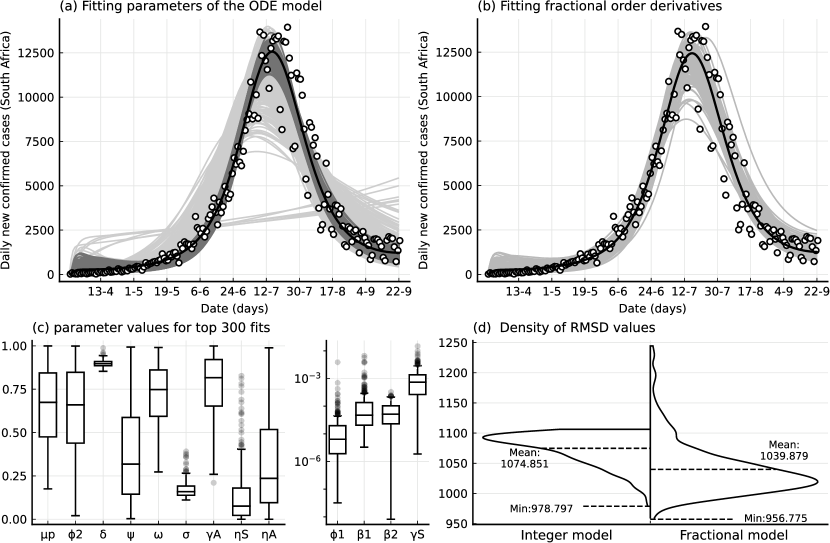
Figure 1: Demonstrating the accuracy of the analyzed model (1), in fitting the daily new confirmed cases obtained from CSSE [23]. (a) The data points are represented by the circles, and the evaluation of errors is carried out by employing the root mean square deviation (RMSD). The light gray curves indicate the results of the model with initial estimates of parameter values and initial conditions. The dark gray curves represent 300 optimal fits, and the black curve shows the best fit with an RMSD of 978.7969. (b) The gray curves represent the results of the model with the optimized order derivatives for the 300 selected best fits, and the black curve shows the best fit, with an RMSD of 956.775. (c) The distributions of selected parameter values are illustrated through boxplot representation. (d) The distribution of error scores for the integer and fractional model (left and right, respectively).

We determine the remaining parameter values and initial conditions through the process of fitting model (1) to the daily new confirmed cases data. Next, we optimize the order derivatives to examine the efficacy of fractional orders in the fitting process. We utilize the root mean square deviation (RMSD) as a measure of the model accuracy, where RMSD$(x,\widehat{x})=\sqrt{\frac{1}{n}\sum_{t=1}^{n}(x_{t}-\widehat{x}_{t})^{2}}$. Here, $n$ denotes the number of data points, $x$ denotes the estimated values, and $\widehat{x}$ denotes the actual values. It is noteworthy that when fitting a model to data, the consideration of biologically or clinically meaningful parameters plays a crucial role. For instance, previous research studies [24, 25] suggest that the parameters $\gamma_{S}$ and $\gamma_{A}$ should be confined to the range of (0,1), and the parameter $\sigma$ should fall within the range of (0.01, 0.06). Given this point, we have chosen to display a set of fitted results, rather than solely presenting the best fit, to demonstrate the overall efficiency of the model utilizing fractional calculus.

In Figure 1(a), the Bayesian inference method is employed to provide initial estimates for both the parameter values and initial conditions, as the results depicted by the light gray curves. Subsequently, 300 optimal fits are chosen from the results (as illustrated by the dark gray curves), and the black curve represents the best fit with an RMSD of 978.7969. In Figure 1(b), we further optimize the order derivatives for the 300 selected best fits, and their results are depicted by the gray curves, while the black curve shows the best fit with an RMSD of 956.775. Additionally, The boxplot representation in Figure 1(c) portrays the statistical properties of the parameter values utilized in the selected candidates, which can potentially provide valuable insights into fitting parameters in similar compartmental models. Figure 1(d) depicts the density of errors for the 300 selected candidates, categorized into integer orders and fractional orders, represented by the left and right sides of the violin plot, respectively. The results reveal that the mean and minimum errors of the model with fractional orders are comparatively lower than those of the model with integer orders. Nonetheless, it should be noted that there are a few isolated instances where the fractional models fitted worse than the integer-order models. The tables presenting the optimal values of the parameters, initial conditions, and order derivatives, along with their corresponding statistical properties such as mean, standard deviation, and median can be found in Table 2 and Tabel 3.

Table 2: Statistical properties of the selected values of the parameters and the sensitivity index of $R_{0}$ across all parameters ($\mathcal{S}_{\mathcal{P}}^{R_{0}}$) for their optimized values.

parameters	mean	std	median	optimized value	sensitivity
$\mu$	-	-	-	-	1.0000
$\Lambda$	-	-	-	-	-0.7169
$\mu_{p}$	0.6566	0.2165	0.6747	0.6642	-0.1361
$\phi_{1}$	3.49e-5	0.0002	6.37e-6	9.09e-7	0.0000
$\phi_{2}$	0.6268	0.2456	0.6603	0.0634	0.0000
$\beta_{1}$	0.0002	0.0007	4.72e-5	7.69e-6	0.1382
$\beta_{2}$	6.90e-5	5.96e-5	5.17e-5	1.68e-5	0.8618
$\delta$	0.8988	0.0193	0.8973	0.9338	0.5860
$\psi$	0.3749	0.2765	0.3183	0.0081	-0.0081
$\omega$	0.7214	0.1725	0.7484	0.9677	0.0280
$\sigma$	0.1711	0.0477	0.1593	0.3194	-0.8957
$\gamma_{S}$	0.0011	0.0015	0.0007	0.0002	-0.0007
$\gamma_{A}$	0.7747	0.1725	0.8165	0.8667	-0.0195
$\eta_{S}$	0.1344	0.1639	0.0760	0.2188	0.1276
$\eta_{A}$	0.3206	0.2733	0.2359	0.9048	0.0105

Table 3: Statistical properties of the selected values for initial conditions and order derivatives, and their optimized values.

initial conditions	mean	std	median	optimized value
$S(0)$	45395.9	14711.4	41078.4	90336.8
$E(0)$	7.42043	23.2615	0.00044	4.297e-6
$I_{A}(0)$	153.791	87.4703	156.002	231.888
$W(0)$	94.6353	79.8807	77.6268	220.056
order derivatives	mean	std	median	optimized value
$\alpha_{S}$	0.995353	0.004721	0.996313	1.000000
$\alpha_{E}$	0.998563	0.008932	1.000000	0.998880
$\alpha_{I_{A}}$	0.977973	0.060090	1.000000	1.000000
$\alpha_{I_{S}}$	0.999547	0.004181	1.000000	0.980835
$\alpha_{R}$	0.749677	0.016673	0.750000	0.750032
$\alpha_{W}$	0.973167	0.032041	0.987370	0.964870
$\alpha_{N}$	0.996496	0.004506	0.999530	1.000000

4.1 Sensitivity analysis of the basic reproduction number

The purpose of this section is to examine the influence of different factors on the transmission of epidemic diseases. By assessing the sensitivity of $R_{0}$ to various parameters, such as social distancing measures, policymakers can make informed decisions regarding public health interventions. Furthermore, this methodology allows for the identification of parameters that have the most significant impact on disease propagation. To assess the effects of minor variations in parameter $\mathcal{P}$ on the basic reproduction number $R_{0}$, we introduce the forward normalized sensitivity index of $R_{0}$ for $\mathcal{P}$, which can be mathematically formulated as:

$$\mathcal{S}_{\mathcal{P}}^{R_{0}}=\frac{\partial R_{0}}{\partial\mathcal{P}}\frac{\mathcal{P}}{R_{0}}.$$

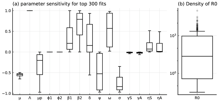
Figure 2: (a) The boxplots of the sensitivity indices for $R_{0}$ associated with the selected parameter values, and (b) the distribution of $R_{0}$ for these values.

If the sensitivity index of $\mathcal{S}_{\mathcal{P}}^{R_{0}}$ is positive, it indicates an increase in the value of the basic reproduction number $R_{0}$ with respect to the parameter $\mathcal{P}$. Conversely, if the value of $R_{0}$ decreases in response to changes in the parameter $\mathcal{P}$, the sensitivity index will be negative. We have conducted an analysis of the sensitivity of the basic reproduction number, $R_{0}$, with respect to the optimized parameters. The computed sensitivity indices for $R_{0}$ have been demonstrated in Table 2. In addition, we illustrate the distribution of sensitivity indices of the selected values of parameters on $R_{0}$ through boxplots, together with the density of $R_{0}$ for these values with considering mean of $N$, in Figure 2. Our analysis revealed that only the parameter $\delta$, which represents the proportion of symptomatic infectious individuals, exhibited mostly positive but sometimes negative sensitivity, while the other parameters maintained their sign of sensitivity indices. Additionally, it would be interesting to discuss the sensitivity of the parameters associated with pathogenic viruses, namely $\mu_{P}$, $\phi_{1}$, $\beta_{1},\eta_{S}$, and $\eta_{A}$. The sensitivity index for $\phi_{1}$ is zero as it is not in equation (3), and as expected, for $\mu_{P}$ is always negative, while for $\beta_{1},\eta_{S}$, and $\eta_{A}$ is positive.

4.2 Numerical methods and implementation

The numerical analyses in this study were carried out using the Julia programming language and the high-performance computing system PUHTI at the Finnish IT Center for Science (CSC). To solve fractional differential equations, the FdeSolver.jl package (v 1.0.7) was utilized, which implements predictor-corrector algorithms and product-integration rules [26]. Parameter estimation was performed using Bayesian inference and Hamiltonian Monte Carlo (HMC) with the Turing.jl package, and ODEs were solved using the DifferentialEquations.jl package. The order of derivatives was optimized using the function (L)BFGS, which employs the (Limited-memory) Broyden–Fletcher–Goldfarb–Shanno algorithm from the Optim.jl package in combination with FdeSolver.jl.

4.3 Data and code availability

All computational results for this article, including all data and code used for running the simulations and generating the figures are available on GitHub and accessible via
https://github.com/moeinkh88/Covid_Shedding.git.

5 Conclusion

Our study presents a modified approach to modeling COVID-19 transmission dynamics by introducing a fractional model that incorporates pathogens in the environment as a shedding effect. This approach offers a more comprehensive representation of disease transmission dynamics by capturing the complex and heterogeneous nature of disease transmission dynamics. Our model also accounts for a variable population and birth rate and employs incommensurate fractional order derivatives in ODEs.

Our analysis accurately computes the basic reproduction number and demonstrates the global stability of the disease-free equilibrium point. We use numerical simulations fitted to real data from South Africa to show the efficacy of our proposed model. Furthermore, we compare the performance of our model with fractional orders against those with integer orders. Our results indicate that fractional models perform more flexibly. We also provide a range of reliable values for the initial conditions, model parameters, and order derivatives. Additionally, our analysis examines the sensitivity of the model parameters.

Overall, our study offers valuable insights into COVID-19 transmission dynamics and has the potential to inform the development of effective measures to control the ongoing pandemic and prevent future outbreaks. We hope that our findings will contribute to a better understanding of this complex disease and its transmission dynamics.

Declaration of Competing Interest

The authors declare no conflict of interest.

References

- [1] Faïçal Ndaïrou, Iván Area, Juan J. Nieto, and Delfim F.M. Torres. Mathematical modeling of covid-19 transmission dynamics with a case study of wuhan. Chaos, Solitons & Fractals, 135:109846, 2020.
- [2] Sebastien Boyer, Borin Peng, Senglong Pang, Véronique Chevalier, Veasna Duong, Christopher Gorman, Philippe Dussart, Didier Fontenille, and Julien Cappelle. Dynamics and diversity of mosquito vectors of japanese encephalitis virus in kandal province, cambodia. Journal of Asia-Pacific Entomology, 23(4):1048–1054, 2020.
- [3] Muhammad Altaf Khan, Yasir Khan, and Saeed Islam. Complex dynamics of an seir epidemic model with saturated incidence rate and treatment. Physica A: Statistical mechanics and its applications, 493:210–227, 2018.
- [4] Xingbo Liu and Lijuan Yang. Stability analysis of an seiqv epidemic model with saturated incidence rate. Nonlinear Analysis: Real World Applications, 13(6):2671–2679, 2012.
- [5] Swati and Nilam. Fractional order sir epidemic model with beddington–de angelis incidence and holling type ii treatment rate for covid-19. Journal of Applied Mathematics and Computing, 68(6):3835–3859, Dec 2022.
- [6] Chunyan Ji. The threshold for a stochastic hiv-1 infection model with beddington-deangelis incidence rate. Applied Mathematical Modelling, 64:168–184, 2018.
- [7] Adnane Boukhouima, Khalid Hattaf, and Noura Yousfi. Dynamics of a fractional order hiv infection model with specific functional response and cure rate. International Journal of Differential Equations, 2017:8372140, Aug 2017.
- [8] El Mehdi Lotfi, Mehdi Maziane, Khalid Hattaf, and Noura Yousfi. Partial differential equations of an epidemic model with spatial diffusion. International Journal of Partial Differential Equations, 2014:186437, Feb 2014.
- [9] Iván Area, Francisco J Fernández, Juan J Nieto, and F Adrián F Tojo. Concept and solution of digital twin based on a stieltjes differential equation. Mathematical Methods in the Applied Sciences, 45(12):7451–7465, 2022.
- [10] Samuel Mwalili, Mark Kimathi, Viona Ojiambo, Duncan Gathungu, and Rachel Mbogo. Seir model for covid-19 dynamics incorporating the environment and social distancing. BMC Research Notes, 13(1):1–5, 2020.
- [11] Anuraj Singh and Preeti Deolia. Covid-19 outbreak: a predictive mathematical study incorporating shedding effect. Journal of Applied Mathematics and Computing, 69(1):1239–1268, 2023.
- [12] Salisu M Garba, Jean M-S Lubuma, and Berge Tsanou. Modeling the transmission dynamics of the covid-19 pandemic in south africa. Mathematical biosciences, 328:108441, 2020.
- [13] Faïçal Ndaïrou and Delfim F. M. Torres. Mathematical analysis of a fractional covid-19 model applied to wuhan, spain and portugal. Axioms, 10(3), 2021.
- [14] Faïçal Ndaïrou, Iván Area, Juan J. Nieto, Cristiana J. Silva, and Delfim F.M. Torres. Fractional model of covid-19 applied to galicia, spain and portugal. Chaos, Solitons & Fractals, 144:110652, 2021.
- [15] Meghdad Saeedian, Moein Khalighi, Nahid Azimi-Tafreshi, Gholamreza Jafari, and Marcel Ausloos. Memory effects on epidemic evolution: The susceptible-infected-recovered epidemic model. Physical Review E, 95:022409, 2017.
- [16] Faïçal Ndaïrou, Moein Khalighi, and Leo Lahti. Ebola epidemic model with dynamic population and memory. Chaos, Solitons & Fractals, 170:113361, 2023.
- [17] Lazarus Kalvein Beay and Nursanti Anggriani. Dynamical analysis of a modified epidemic model with saturated incidence rate and incomplete treatment. Axioms, 11(6), 2022.
- [18] Yanan Zhao and Daqing Jiang. The threshold of a stochastic sirs epidemic model with saturated incidence. Applied Mathematics Letters, 34:90–93, 2014.
- [19] Xiangyun Shi, Xueyong Zhou, and Xinyu Song. Dynamical behavior of a delay virus dynamics model with ctl immune response. Nonlinear Analysis: Real World Applications, 11(3):1795–1809, 2010.
- [20] Dan Li and Wanbiao Ma. Asymptotic properties of a hiv-1 infection model with time delay. Journal of Mathematical Analysis and Applications, 335(1):683–691, 2007.
- [21] Oyoon Abdul Razzaq, Najeeb Alam Khan, Muhammad Faizan, Asmat Ara, and Saif Ullah. Behavioral response of population on transmissibility and saturation incidence of deadly pandemic through fractional order dynamical system. Results in Physics, 26:104438, 2021.
- [22] P. van den Driessche and James Watmough. Reproduction numbers and sub-threshold endemic equilibria for compartmental models of disease transmission. Mathematical Biosciences, 180(1):29–48, 2002.
- [23] Ensheng Dong, Hongru Du, and Lauren Gardner. An interactive web-based dashboard to track covid-19 in real time. The Lancet Infectious Diseases, 20(5):533–534, 2020.
- [24] Calistus N. Ngonghala, Enahoro Iboi, Steffen Eikenberry, Matthew Scotch, Chandini Raina MacIntyre, Matthew H. Bonds, and Abba B. Gumel. Mathematical assessment of the impact of non-pharmaceutical interventions on curtailing the 2019 novel coronavirus. Mathematical Biosciences, 325:108364, 2020.
- [25] Neil Ferguson, Daniel Laydon, Gemma Nedjati Gilani, Natsuko Imai, Kylie Ainslie, Marc Baguelin, Sangeeta Bhatia, Adhiratha Boonyasiri, ZULMA Cucunuba Perez, Gina Cuomo-Dannenburg, et al. Report 9: Impact of non-pharmaceutical interventions (npis) to reduce covid19 mortality and healthcare demand. 2020.
- [26] Moein Khalighi, Giulio Benedetti, and Leo Lahti. Fdesolver: A julia package for solving fractional differential equations. arXiv:2212.12550, 2022.