Sharpend Cosine Similarity based Neural Network for Hyperspectral Image Classification

Abstract

Hyperspectral Image Classification (HSIC) is a difficult task due to high inter and intra-class similarity and variability, nested regions, and overlapping. 2D Convolutional Neural Networks (CNN) emerged as a viable network whereas, 3D CNNs are a better alternative due to accurate classification. However, 3D CNNs are highly computationally complex due to their volume and spectral dimensions. Moreover, down-sampling and hierarchical filtering (high frequency) i.e., texture features need to be smoothed during the forward pass which is crucial for accurate HSIC. Furthermore, CNN requires tons of tuning parameters which increases the training time. Therefore, to overcome the aforesaid issues, Sharpened Cosine Similarity (SCS) concept as an alternative to convolutions in a Neural Network for HSIC is introduced. SCS is exceptionally parameter efficient due to skipping the non-linear activation layers, normalization, and dropout after the SCS layer. Use of MaxAbsPool instead of MaxPool which selects the element with the highest magnitude of activity, even if it’s negative. Experimental results on publicly available HSI datasets proved the performance of SCS as compared to the convolutions in Neural Networks.

I Introduction

Hyperspectral Image Classification (HSIC) has been an extensively studied area of research for decades for many applications [1, 2, 3, 4, 5]. HSIC task requires assigning a unique class label to a set of pixels according to the information presented in HSI [6, 7, 8]. Early HSIC approaches are based on handcrafted features which are extracted from spectral (color, intensity, etc.) or spatial (texture, shape, etc.) information or their combination. Among the handcrafted features, HoG, texture, and color features are widely employed. However, the classification performance largely deteriorated since these approaches are not able to extract rich semantic features from HSI.

To overcome the aforesaid limitations, several unsupervised feature-learning techniques have been proposed. Such techniques focus on learning a set of basis functions used for feature encoding for an image [6]. These approaches can learn more discriminative information thus suitable for representing the information. However, the discriminative performance is still limited as these techniques do not make use of class information, hence, do not well represent distinguishable features among different classes [9].

To overcome the aforesaid limitations, deep learning approaches have been proposed, especially Convolutional Neural Network (CNN) [10, 11, 12, 13]. CNNs are able to use class information to learn discriminative features, thus the features learned by CNN are more robust and discriminative for HSIC. However, due to the down-sampling and hierarchical filtering processes, the high frequency (i.e., texture features) gradually needs to be smoothened during the forward processes [14]. Thus, to some extent, CNN architecture can be considered a low-frequency pathway for HSIC. Moreover, traditional CNN models require tons of parameters to train the model which increases the training time. Therefore, to overcome the aforesaid issues, this work proposed the use of the Sharpened Cosine Similarity (SCS) concept as an alternative to convolutions in a neural network. More specifically, the following benefits can be obtained using SCS instead of convolutions in neural networks. SCS appears to be parameter efficiency and architecture simplicity due to the nonexistence of nonlinear activation layers, dropout, and normalization layers, like batch normalization or layer normalization, after SCS layers. Use AbsMaxpool instead of Maxpool. It selects the element with the highest magnitude of activity, even if it’s negative.

II Literature Review

High-level earth observation using HSI has become cutting-edge research. Hence HSIC has drawn widespread attention and brought several state-of-the-art methodologies since its emergence [15]. However, most of the early approaches only considered shallow processing which requires feature engineering prior to the classification. Moreover, shallow-level processing requires extensive parameter tuning, settings, and experience which affects the learning capabilities. Therefore, during the past decade, deep learning such as CNNs and similar methodologies have been proposed.

The works [16, 17] proposed an HSIC method based on deep pyramid residual and capsule networks. Similarly, the work [18] proposed a spectral-spatial residual network in which the residual blocks were used for identity mapping to connect 3D CLs whereas the work [19] proposed an unsupervised HSIC method to better explore the residual CLs. The work [20] proposed a 3D CNN network for both spatial-spectral feature learning and classification. The work [21] proposed a mini-batch Graph CNN (miniGCN) which addresses the complexity of graph computation and feature fusion extracted by CNN and miniGCN as an end-to-end network.

From the above discussion, one can conclude that features learned by CNN are more robust and discriminative for HSIC as compared to the other methods. However, due to the down-sampling and hierarchical filtering process, the high-frequency features gradually need to be smoothened during the forward pass. To some extent, these features are considered crucial for accurate classification, therefore, CNN architecture is referred to as a low-frequency pathway. Moreover, parameter explosion is yet another issue that increases the computational time. To overcome the aforesaid issues, this work implemented an SCS as an alternative to Convolutional Layers (CLs) for HSIC. There are a number of benefits that can be obtained using SCS instead of CLs in neural networks.

For instance, SCS appears to be parameter efficient, and its architecture simplicity. It’s not about the accuracy records but it’s killing in parameter efficiency leaderboard. Skip the non-linear activation layers, dropout layers, and normalization layers after SCS. SCS uses Abs Max-pool instead of Max-pool which selects the element with the highest magnitude of activity even if it’s negative. Thus, in a nutshell, the SCS works better in terms of the computational cost requires to train a DNN as compared to deep CNNs.

III Methodology

Let us consider an HSI $\textbf{X}\in\mathcal{R}^{(M\times{N})\times{B}}$ where $(M\times N)$ represents the spatial region over the Earth’s surface and $B$ refers to be the number of spectral bands exists in HSI. All $x_{ij}\in\textbf{X}$ pixels of HSI are classified into $C$ disjoint land-cover classes denoted as $Y=(y_{1},y_{2},\dots,y_{n})$. Each $x_{ij}\in\textbf{X}$ (where $i=1,2,\dots,M$ and $j=1,2,\dots,N$) define a land-cover pixel as a spectral vector $x_{ij}=[x_{i,j,1},x_{i,j,2},\dots,x_{i,j,B}]\in\textbf{X}$ contain $B$ number of values.

Moreover, to process the spatial information, the patch extraction process is carried out as a preprocessing step where the HSI cube $\textbf{x}_{i,j}\in\mathcal{R}^{(k\times k)\times B}$ with the neighboring regions of size $k\times k$ centered at targeted pixel $(i,j)$. joint spectral-spatial features can increase the discriminative power of any model, thus the spectral-spatial cubes $\textbf{x}_{i,j}\in\mathcal{R}^{(k\times k)\times B}$ are extracted from raw data and stacked into $X$ before feature extraction. Finally, the training and test samples were selected for each class.

Convolution in Neural Network is a sliding dot product between the patch of the image and the kernel aligned which may not be a good similarity metric and thus may skip some important information which makes it an inappropriate feature detector. However, normalizing both to a magnitude of $1$, thus it will turn to cosine similarity. The cosine of two non-zero vectors can be derived by using the Euclidean distance as $k\cdot x_{i}=||k||~{}||x_{i}||cos\theta$, given $k$ and $x_{i}$, the cosine similarity $cos(\theta)$ can be computed as $cos(\theta)=\frac{k\cdot x_{i}}{||k||~{}||x_{i}||}=\frac{\sum_{i=1}^{n}k_{i}~{}x_{i}}{\sqrt{\sum_{i=1}^{n}k_{i}^{2}}\sqrt{\sum_{i=1}^{n}x_{i}^{2}}}$.

The resulting similarity ranges from $-1$ to $1$, where $-1$ means that the kernel and the image patch are exactly opposite and $0.5$ means intermediate similarity or dissimilarity among the kernel and image, whereas, $1$ means that the kernel and the patch are aligned. The main issue in cosine similarity is a very small magnitude between the kernel and the image patch which in principle desired to be magnitude in variance. However, keeping it to an extreme may end up gathering background or noise rather than foreground information. Thus, extra parameters can help to overcome the aforesaid issues.

Therefore, the SCS was initiated, which is a stridden operation similar to convolution that extracts features from an image patch. SCS is similar to the convolutional process, however, have some important differences. In practice, the convolution is a stridden dot product among the kernel $k$ and the image patch $x_{i}$ as $k\cdot x_{i}$, whereas in cosine similarity, the image patch and kernel are normalized to have a magnitude of $1$ before the dot product is taken. It is so named because, in two dimensions, it gives the cosine of the angle between the image patch and the kernel as $\frac{k\cdot x_{i}}{||k||~{}||x_{j}||}$. Therefore, the cosine can be sharpened by raising the magnitude of the result to a power $p$ while maintaining the sign as $sign(k\cdot x_{i})\left|\frac{k\cdot x_{i}}{||k||~{}||x_{i}||}\right|^{p}$. This measure can become numerically unstable if ever the magnitude of the image patch or kernel gets too close to zero. In practice, the kernel magnitude doesn’t get too small and doesn’t need $q$, however, maybe a good practice to have a small constraint on it as well, i.e., $sign(k\cdot x_{i})\left|\frac{k\cdot x_{i}}{||k+q||~{}||x_{i}||}\right|^{p}$.

$$SCS(k,x_{i})=sign(k\cdot x_{i})\bigg{(}\frac{k\cdot x_{i}}{(||k||+q)(||x_{i}+q||)}\bigg{)}$$ (1)

Similar to the traditional convolutional process in Deep Learning, SCS is also a stride operation that takes features as an output from an input image patch. However, before calculating the straight dot product, the kernel and image patch are adjusted to have a magnitude of 1 that produce the sharpened cosine similarity or some literature refers to it as sharpened cosine normalization. SCS operation extracts feature from image patches for which sharpening exponents must be learned for each unit which can be sharpened by raising it to a power of an exponent. The aforementioned procedure outperformed and is faster than a convolutional process in any neural network by 10 to 100 times due to the fewer number of required parameters, without the normalization and activation function.

Apart from the SCS process, as compared to the pooling that is used to downsample the data, absolute max-pooling is used to update the filter in backpropagation until an appropriate value of features is obtained from the given patch. Moreover, as compared to simple pooling, absolute maxpooling chooses the highest magnitude even if a certain element has a negative value.

The overall model is trained using 250 epochs, 256 batch sizes, and a 0.001 learning rate. The learning rate has a strong influence on the pace of learning any Deep Model that determines the number of movements required to minimize the loss of function value whereas the momentum is used to enhance the accuracy and model’s training speed. The RMS and momentum prop optimizer combined model is trained using the Adam optimizer. TensorFlow-based Keras tuner library is called to fine-tune the hyperparameters for SCS-Net which ultimately makes the overall model robust and comparative as compared to the other state-of-the-art models. The motivation behind using the Adam optimizer is its efficiency in consuming less memory and computational efficiency. The complete architecture is presented in Figure 1.

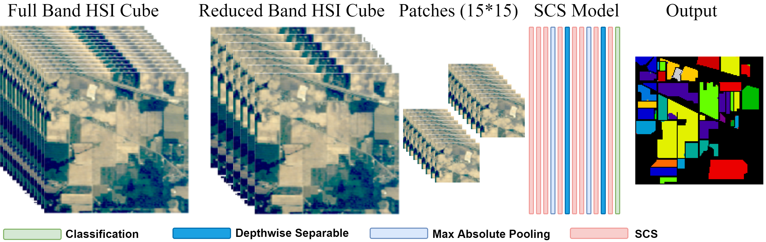
Figure 1: Workflow of SCS pipeline.

IV Experimental Results and Discussion

This section discusses the experimental datasets used to evaluate the proposed pipeline along with the comparative methods proposed in recent years. Moreover, this section presents the details regarding the experimental settings, results, and discussion together with the experimental results as compared to the state-of-the-art methods proposed in recent years. For experimental evaluation, two publicly available HSI datasets have been used. These datasets were acquired at different times, locations, and sensors.

The works published in the literature present comprehensive results to highlight the pros and cons as compared to state-of-the-art works however, to some extent, all the works may have different experimental settings such as, the number or percentage of training, validation, and test samples may remain the same but their geographical locations may differ (due to the random selection nature) as these methods may have run in different times or may have executed on different machines. Therefore, to make the comparison fair among different works, one must need to have the same number/percentage and geographical locations of training, validation, and test samples. Thus, in this work, the first experimental settings, i.e., the percentage of training, validation, and test samples along with their geographical locations remain the same as all the comparative methods along with the SCS pipeline are executed in one single run.

The experimental results presented in this section have been obtained using Google Colab with a Graphical Process Unit with 358$+$ GB of storage and $25GB$ of RAM. For all the experimental results presented in this section the training, validation, and test samples are randomly selected as 40%/30%/30%. For fair comparative analysis, all three models have been executed at once with one-time randomly selected samples. The presented results are obtained using $15\times 15$ patch size along with the $15$ most informative bands selected through PCA. As far as the training parameters for 3D CNN and Hybrid models, the weights are initially randomized and later optimized using backpropagation with Adam optimizer and softmax loss function. The overall training and validation loss and accuracy for all three models are presented in Figure 2.

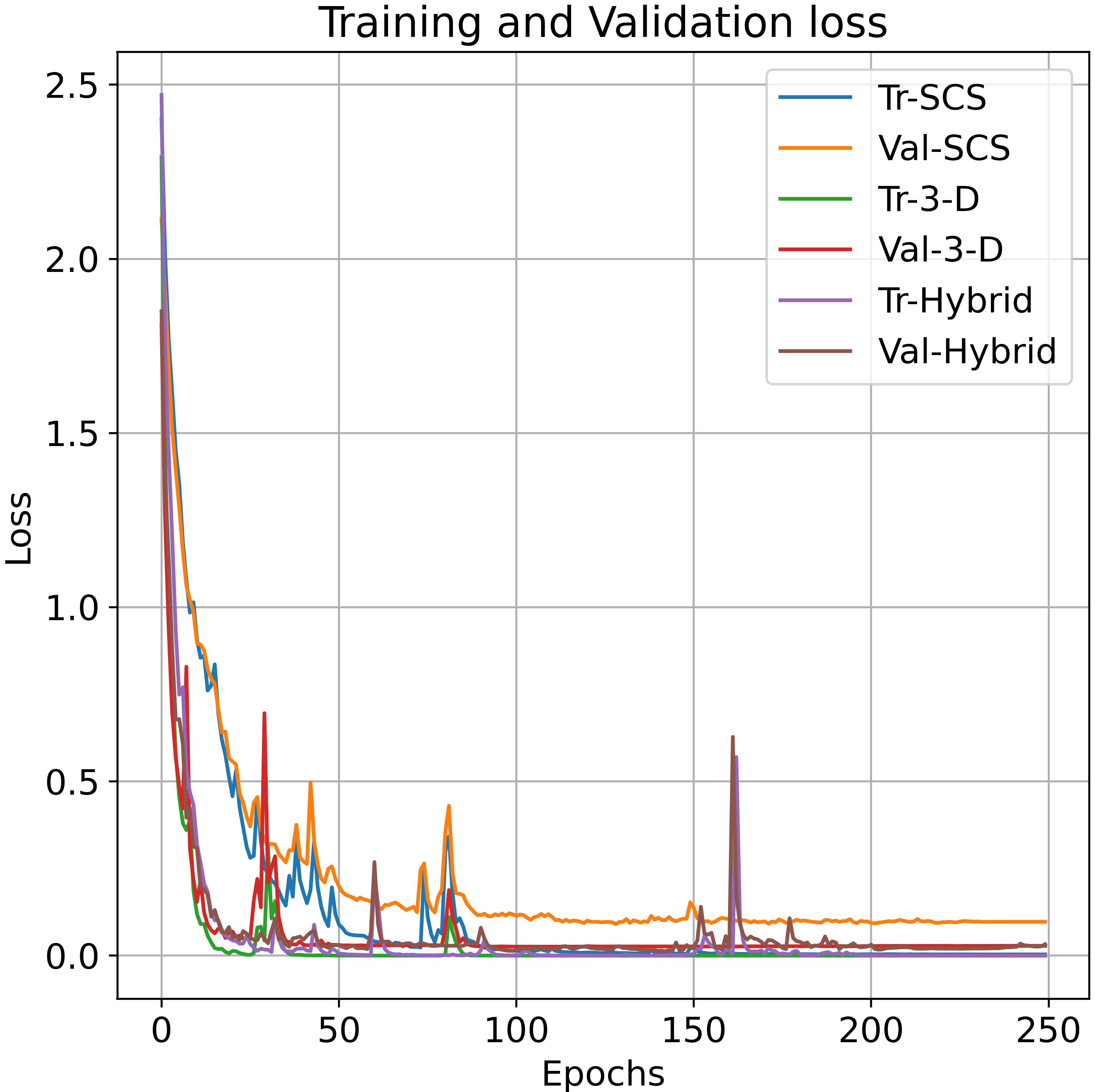
(a) Loss

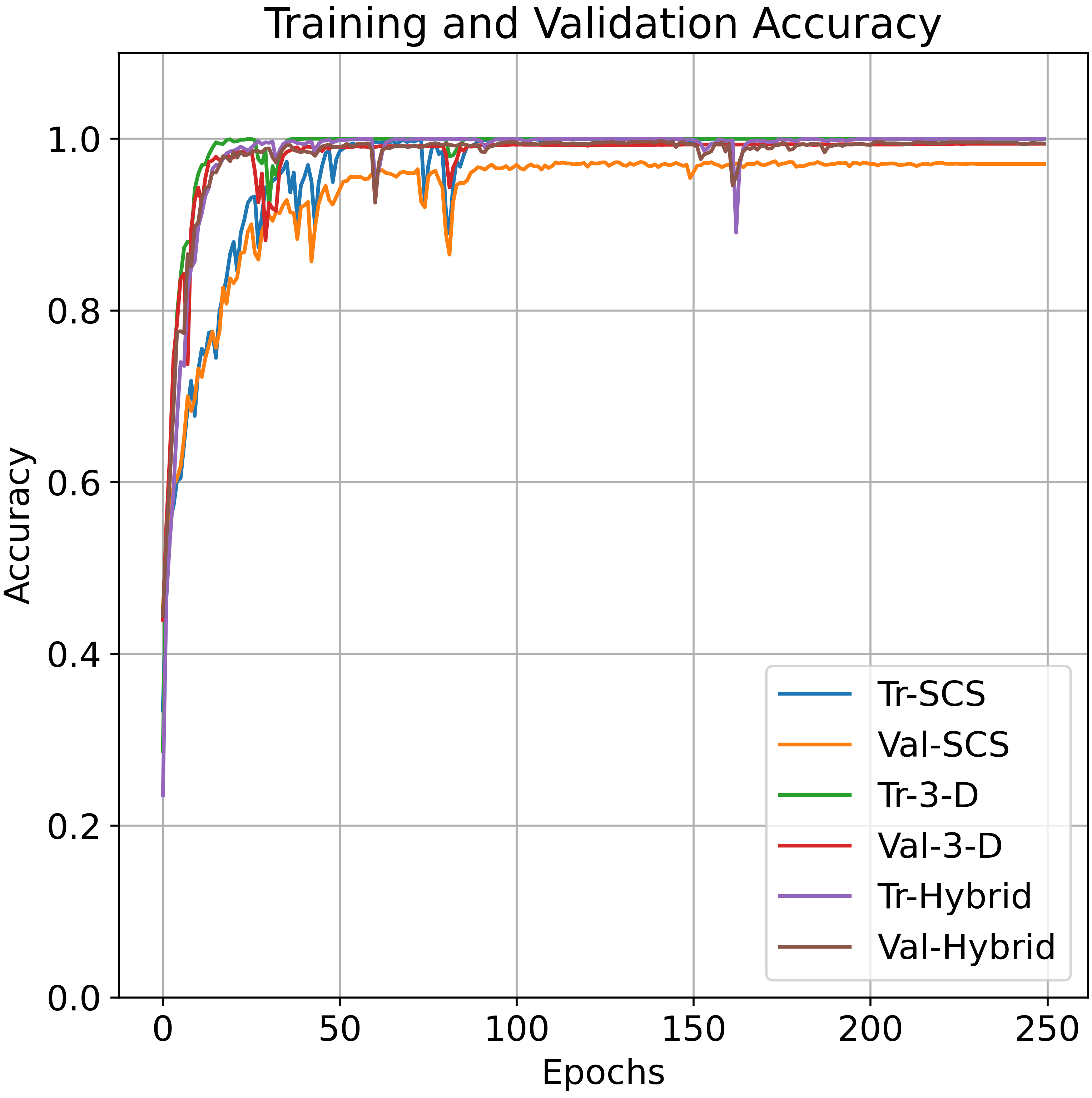
(b) Accuracy

Figure 2: Training and Validation Loss and Accuracy of SCS network along with 3D-CNN and Hybrid CNN.

The experimental results presented in Figure 3 and Table I for both IP and SA datasets are obtained using the overall, average accuracy, and Kappa coefficient. Kappa computes the mutual information regarding a strong agreement among the classification and ground-truth maps whereas Average and Overall accuracy compute the average class-wise classification performance and the correctly classified samples out of the total test samples, respectively.

(a) SCS

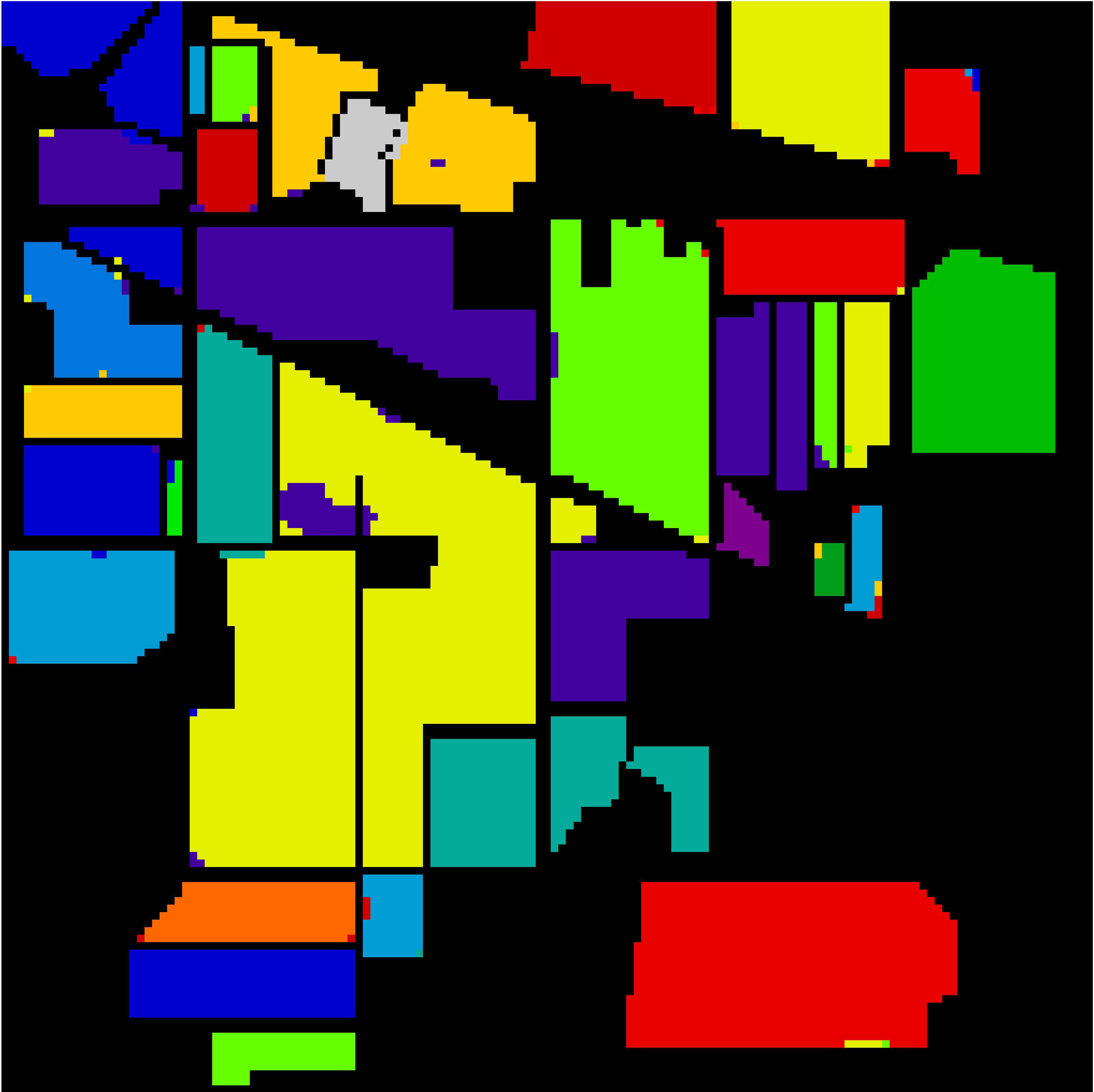
(b) 3D

(c) Hybrid

(d) SCS

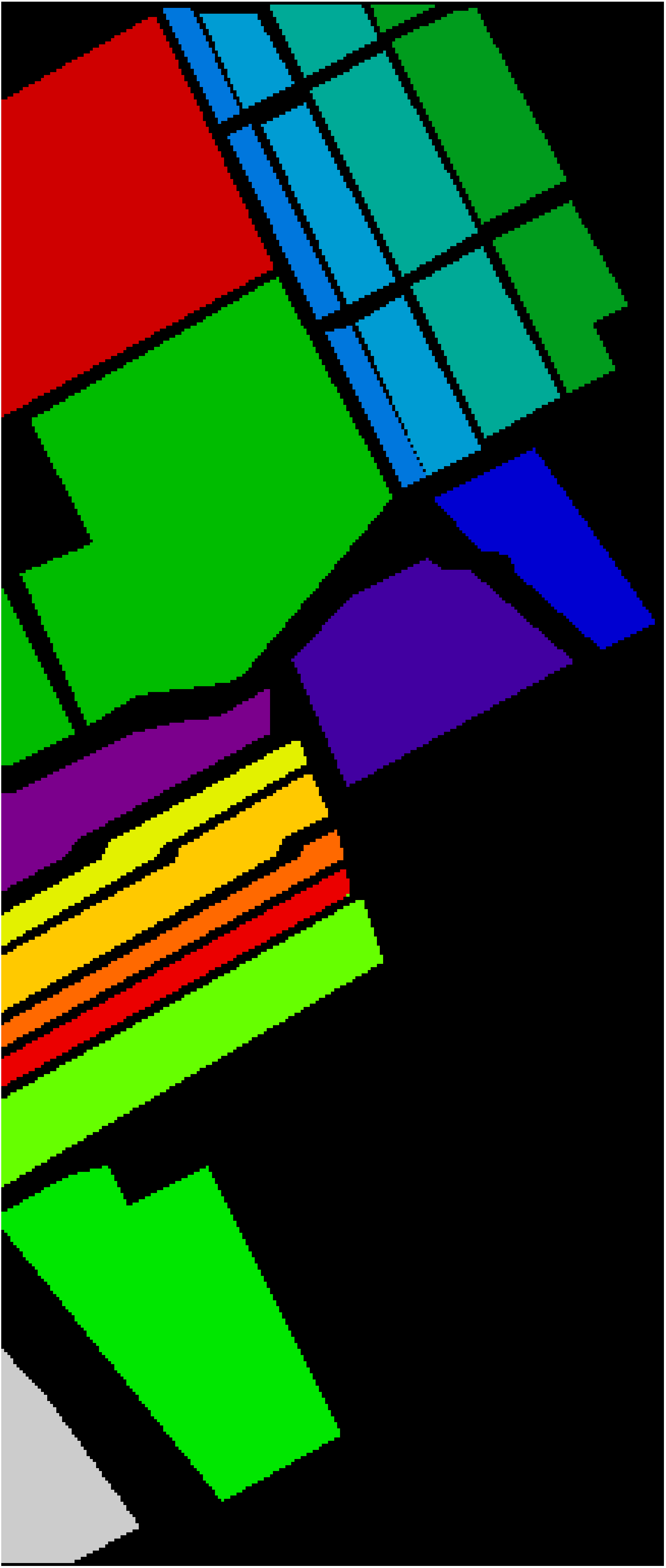
(e) 3D

(f) Hybrid

Figure 3: Geographical maps for Indian Pines (IP) and Salinas (SA) datasets. Per-class results are presented in Table I.

TABLE I: Classification performance obtained over $15\times 15$ patch sizes.

Indian Pines				Salinas
Class	SCS	3D CNN	Hybrid	Class	SCS	3D CNN	Hybrid
Alfalfa	92.5925	100	100	Weeds 1	100	100	100
Corn-notill	93.2322	97.1995	97.0828	Weeds 2	100	100	100
Corn-mintill	96.5863	99.5983	100	Fallow	100	100	100
Corn	84.5070	97.1830	99.2957	Fallow RP	100	100	100
Grass-pasture	93.7931	95.8620	98.9655	Fallow smooth	99.9253	100	99.9253
Grass-trees	99.0867	99.7716	100	Stubble	100	100	100
Grass-mowed	94.1176	88.2352	88.2352	Celery	100	100	100
Hay-windrowed	99.3031	100	100	Grapes untrained	99.9645	100	99.8935
Oats	66.6666	75.0000	66.6666	Soil vinyard develop	100	100	100
Soybean-notill	93.3104	97.5986	98.6277	Corn Weeds	99.9389	100	99.7559
Soybean-mintill	98.3706	98.7101	99.5926	Lettuce 4wk	99.6254	100	100
Soybean-clean	87.9213	97.4719	97.7528	Lettuce 5wk	100	100	100
Wheat	99.1869	98.3739	100	Lettuce 6wk	100	100	100
Woods	99.8682	98.9459	99.3412	Lettuce 7wk	100	99.8130	100
Buildings	95.2586	99.1379	100	Vinyard untrained	100	100	99.4771
Stone-Steel	92.8571	98.2142	100	Vinyard trellis	100	100	100
Kappa	95.3421	98.0899	98.8505	Kappa	99.9753	99.9958	99.8765
Overall	95.9186	98.3252	98.9918	Overall	99.9778	99.9963	99.8891
Average	92.9161	96.3314	96.5975	Average	99.9658	99.9883	99.9407

TABLE II: Salinas Dataset: The comparative methods include Multi-layered Perceptron (MLP) [22], Multinomial Logistic Regression (MLR) [23], Random Forest (RF) [24], Support Vector Machine (SVM) [25], 1D CNN [11], 2D CNN [26], 3D CNN [13], Hybrid CNN [27], Bayesian CNN (1D, 2D, and 3D BCNN) [12]. All these methods are retrained using the same number of training samples to make the comparison fair and reliable.

Class

MLP

MLR

RF

SVM

1D CNN

2D CNN

3D CNN

Hybrid CNN

1D-BCNN

2D-BCNN

3D-BCNN

SCS

Broccoli green weeds 1

98.16$\pm$1.94

98.26$\pm$0.61

97.71$\pm$1.94

97.59$\pm$1.31

99.00$\pm$0.42

99.85$\pm$0.15

100$\pm$0.00

100$\pm$0.00

99.8 $\pm$0.22

99.55 $\pm$0.45

100 $\pm$0.00

100$\pm$0.00

Broccoli green weeds 2

99.48$\pm$0.40

99.78$\pm$0.07

99.83$\pm$0.07

99.35$\pm$0.45

99.55$\pm$0.00

94.15$\pm$1.45

100$\pm$0.00

100$\pm$0.00

99.97 $\pm$0.02

99.72 $\pm$0.28

100 $\pm$0.00

100$\pm$0.00

Fallow

96.89$\pm$1.76

94.94$\pm$1.82

93.74$\pm$3.59

96.88$\pm$2.08

97.79$\pm$0.56

99.62$\pm$0.03

100$\pm$0.00

100$\pm$0.00

99.68 $\pm$0.21

99.89 $\pm$0.11

100 $\pm$0.00

100$\pm$0.00

Fallow rough plow

99.44$\pm$0.31

99.24$\pm$0.38

97.06$\pm$3.00

98.98$\pm$0.61

98.76$\pm$0.96

99.86$\pm$0.14

100$\pm$0.00

100$\pm$0.00

99.71 $\pm$0.01

99.89 $\pm$0.11

99.61 $\pm$0.18

100$\pm$0.00

Fallow smooth

97.50$\pm$1.15

97.36$\pm$1.21

96.25$\pm$0.99

97.87$\pm$0.72

96.98$\pm$1.18

99.79$\pm$0.06

100$\pm$0.00

99.93$\pm$0.07

98.51 $\pm$1.51

100 $\pm$0.00

99.91 $\pm$0.06

99.92$\pm$0.08

Stubble

99.52$\pm$0.22

99.57$\pm$0.18

98.73$\pm$0.99

99.43$\pm$0.40

99.80$\pm$0.13

99.73$\pm$0.21

100$\pm$0.00

100$\pm$0.00

99.97 $\pm$0.00

100 $\pm$0.00

100 $\pm$0.00

100$\pm$0.00

Celery

99.27$\pm$0.33

99.66$\pm$0.16

99.09$\pm$0.41

99.44$\pm$0.21

99.68$\pm$0.09

99.09$\pm$0.15

100$\pm$0.00

100$\pm$0.00

99.97 $\pm$0.00

100 $\pm$0.00

100 $\pm$0.00

100$\pm$0.00

Grapes untrained

81.16$\pm$5.33

81.89$\pm$3.01

81.85$\pm$2.60

97.53$\pm$1.78

83.43$\pm$3.15

92.31$\pm$1.01

100$\pm$0.00

99.89$\pm$0.00

86.61 $\pm$5.95

9997 $\pm$0.03

99.88 $\pm$0.12

99.96$\pm$0.04

Soil vinyard develop

99.34$\pm$0.43

99.86$\pm$0.07

98.90$\pm$0.44

99.39$\pm$0.52

99.26$\pm$0.43

99.84$\pm$0.06

100$\pm$0.00

100$\pm$0.00

99.96 $\pm$0.01

100 $\pm$0.00

100 $\pm$0.00

100$\pm$0.00

Corn senesced green weeds

89.33$\pm$2.19

88.50$\pm$2.12

85.53$\pm$1.96

91.13$\pm$1.74

93.49$\pm$2.15

96.19$\pm$2.81

100$\pm$0.00

99.76$\pm$0.24

98.59 $\pm$0.48

99.82 $\pm$0.18

100 $\pm$0.00

99.93$\pm$0.07

Lettuce romaine 4wk

90.02$\pm$3.76

91.95$\pm$3.05

88.16$\pm$4.53

93.93$\pm$1.83

94.48$\pm$1.99

96.82$\pm$0.84

100$\pm$0.00

100$\pm$0.00

98.94 $\pm$0.94

100 $\pm$0.00

100 $\pm$0.00

99.62$\pm$0.38

Lettuce romaine 5wk

97.21$\pm$2.40

99.03$\pm$0.73

97.19$\pm$1.37

99.14$\pm$0.56

99.97$\pm$0.05

99.82$\pm$0.18

100$\pm$0.00

100$\pm$0.00

99.48 $\pm$0.24

99.92 $\pm$0.08

99.91 $\pm$0.03

100$\pm$0.00

Lettuce romaine 6wk

97.66$\pm$1.32

94.39$\pm$8.09

97.79$\pm$1.37

97.39$\pm$2.38

98.25$\pm$0.62

98.42$\pm$1.15

100$\pm$0.00

100$\pm$0.00

99.49 $\pm$0.19

100 $\pm$0.00

99.95 $\pm$0.05

100$\pm$0.00

Lettuce romaine 7wk

91.38$\pm$2.33

92.26$\pm$1.34

90.88$\pm$3.21

91.92$\pm$3.07

91.03$\pm$1.75

96.82$\pm$0.00

100$\pm$0.00

100$\pm$0.00

99.19 $\pm$0.23

99.63 $\pm$0.09

100 $\pm$0.00

100$\pm$0.00

Vinyard untrained

64.87$\pm$8.76

60.89$\pm$3.55

59.21$\pm$4.36

64.20$\pm$2.91

66.41$\pm$7.54

84.74$\pm$1.35

99.81$\pm$0.19

99.48$\pm$0.52

74.95 $\pm$9.27

99.64 $\pm$0.30

99.66 $\pm$0.34

100$\pm$0.00

Vinyard vertical trellis

96.36$\pm$1.20

95.29$\pm$2.48

92.92$\pm$2.26

96.70$\pm$1.84

98.34$\pm$0.57

85.78$\pm$0.39

100$\pm$0.00

100$\pm$0.00

99.56 $\pm$0.24

99.81 $\pm$0.19

100 $\pm$0.00

100$\pm$0.00

OA

89.57$\pm$0.41

89.20$\pm$0.30

88.22$\pm$0.29

91.07$\pm$0.37

90.85$\pm$0.77

94.95$\pm$0.07

99.99$\pm$0.01

99.88$\pm$0.18

93.57 $\pm$0.29

99.88 $\pm$0.08

99.91 $\pm$0.08

99.97$\pm$0.03

AA

93.60$\pm$0.56

93.30$\pm$0.59

92.18$\pm$0.28

94.43$\pm$0.38

94.79$\pm$0.64

96.43$\pm$0.23

99.98$\pm$0.02

99.94$\pm$0.06

97.57 $\pm$0.33

99.87 $\pm$0.07

99.94 $\pm$0.05

99.96$\pm$0.04

$\kappa$

88.38$\pm$0.47

89.20$\pm$0.33

86.86$\pm$0.33

90.03$\pm$0.41

90.85$\pm$0.87

94.95$\pm$0.08

99.99$\pm$0.01

99.87$\pm$0.13

93.57 $\pm$0.32

99.88 $\pm$0.09

99.91 $\pm$0.09

99.97$\pm$0.03

V Experiments with State-of-the-art Models

The section discussed the experimental results of SCS and comparative methods proposed in recent years. This work carryout the comparative results with the same settings, irrespective of the literature, e.g., training and test samples may have the same number or percentage but are selected in different runs which leads to the different geographical locations of training and test samples for different methods. For instance, some samples are close to the decision boundary and are hard to classify (may confuse classification) however, in another random selection run, such samples may not be a part of the training set eventually, making classification easy. Therefore, all the comparative methods must need to be evaluated on the same set of samples rather than different samples. In this work, the training and test samples are selected once only and used to train and test all the models for the same samples.

Here the SCS method is compared with Multi-layered Perceptron (MLP) [22], Multinomial Logistic Regression (MLR) [23], Random Forest (RF) [24], Support Vector Machine (SVM) [25], 1D CNN [11], 2D CNN [26], 3D CNN [13], Hybrid CNN [27], Bayesian CNN (1D, 2D, and 3D BCNN) [12]. All these methods were implemented as per the parameters mentioned in their respective works. The detailed experimental results are presented in Table II for the Salains dataset (due to the page length, other datasets’ results are skipped). Looking into Table II, one can conclude that the pixel-based classification methods i.e., MLR and RF under-performed SVM, however, 1D CNNs performance is superior to other pixel-based spectral classification methods. Whereas, the spatial and spectral-spatial classification methods such as 2D, 3D, and Hybrid methods, respectively outperformed spectral methods. Moreover, SCS performance is similar to spectral-spatial methods’ performance while requiring significantly fewer training parameters, i.e., SCS requires $5624$ training parameters whereas, 3D and Hybrid CNN require $127,104$ training parameters, which is significant.

VI Conclusion

Hyperspectral Image Classification is a difficult task due to high inter and intra-class similarity and variability, nested regions, and overlapping. 2D Convolutional Neural Networks (CNN) emerged as a viable network whereas, 3D CNNs are a better alternative due to accurate classification. However, 3D CNNs are highly computationally complex due to their volume and spectral dimensions. Moreover, down-sampling and hierarchical filtering (high frequency) i.e., texture features need to be smoothed during the forward pass which is crucial for accurate classification. Furthermore, CNN requires tons of tuning parameters which increases the training time. To overcome the aforesaid issues, this work presented a Sharpened Cosine Similarity (SCS) as an alternative to Convolution in neural networks. SCS is exceptionally parameter efficient due to the following reasons: Skip nonlinear activation layer (ReLU, Sigmoid, etc.), Skip normalization and dropout layers, Use of Abs Max-pooling instead of MaxPool which selects the elements with the highest magnitude of activity even if its negative. Several experimental results proved the efficiency of SCS as compared to Convolutional layers.

References

- [1] Z. Saleem, M. H. Khan, M. Ahmad, A. Sohaib, H. Ayaz, and M. Mazzara, “Prediction of microbial spoilage and shelf-life of bakery products through hyperspectral imaging,” IEEE Access, vol. 8, pp. 176 986–176 996, 2020.
- [2] M. H. Khan, Z. Saleem, M. Ahmad, A. Sohaib, H. Ayaz, M. Mazzara, and R. A. Raza, “Hyperspectral imaging-based unsupervised adulterated red chili content transformation for classification: Identification of red chili adulterants,” Neural Computing and Applications, vol. 33, no. 21, pp. 14 507–14 521, 2021.
- [3] H. Ayaz, M. Ahmad, M. Mazzara, and A. Sohaib, “Hyperspectral imaging for minced meat classification using nonlinear deep features,” Applied Sciences, vol. 10, no. 21, 2020. [Online]. Available: https://www.mdpi.com/2076-3417/10/21/7783
- [4] M. H. F. Butt, H. Ayaz, M. Ahmad, J. P. Li, and R. Kuleev, “A fast and compact hybrid cnn for hyperspectral imaging-based bloodstain classification,” in 2022 IEEE Congress on Evolutionary Computation (CEC), 2022, pp. 1–8.
- [5] M. Zulfiqar, M. Ahmad, A. Sohaib, M. Mazzara, and S. Distefano, “Hyperspectral imaging for bloodstain identification,” Sensors, vol. 21, no. 9, 2021. [Online]. Available: https://www.mdpi.com/1424-8220/21/9/3045
- [6] W. Zhang, L. Jiao, F. Liu, J. Liu, and Z. Cui, “Lhnet: Laplacian convolutional block for remote sensing image scene classification,” IEEE Transactions on Geoscience and Remote Sensing, pp. 1–1, 2022.
- [7] M. Ahmad, S. Shabbir, S. K. Roy, D. Hong, X. Wu, J. Yao, A. Khan, M. Mazzara, S. Distefano, and J. Chanussot, “Hyperspectral image classification—traditional to deep models: A survey for future prospects,” IEEE Journal of Selected Topics in Applied Earth Observations and Remote Sensing, vol. 15, pp. 968–999, 2022.
- [8] S. K. Roy, A. Deria, D. Hong, M. Ahmad, A. Plaza, and J. Chanussot, “Hyperspectral and lidar data classification using joint cnns and morphological feature learning,” IEEE Transactions on Geoscience and Remote Sensing, 2022.
- [9] M. Ahmad, U. Ghous, D. Hong, A. M. Khan, J. Yao, S. Wang, and J. Chanussot, “A disjoint samples-based 3d-cnn with active transfer learning for hyperspectral image classification,” IEEE Transactions on Geoscience and Remote Sensing, vol. 60, pp. 1–16, 2022.
- [10] S. Yu, S. Jia, and C. Xu, “Convolutional neural networks for hyperspectral image classification,” Neurocomputing, vol. 219, pp. 88–98, 2017. [Online]. Available: https://www.sciencedirect.com/science/article/pii/S0925231216310104
- [11] D. Hong, L. Gao, J. Yao, B. Zhang, A. Plaza, and J. Chanussot, “Graph convolutional networks for hyperspectral image classification,” IEEE Trans. Geosci. Remote Sens., vol. 59, no. 7, pp. 5966–5978, 2021.
- [12] J. M. Haut, M. E. Paoletti, J. Plaza, J. Li, and A. Plaza, “Active learning with convolutional neural networks for hyperspectral image classification using a new bayesian approach,” IEEE Transactions on Geoscience and Remote Sensing, vol. 56, no. 11, pp. 6440–6461, 2018.
- [13] M. Ahmad, A. M. Khan, M. Mazzara, S. Distefano, M. Ali, and M. S. Sarfraz, “A fast and compact 3-d cnn for hyperspectral image classification,” IEEE Geoscience and Remote Sensing Letters, vol. 19, pp. 1–5, 2022.
- [14] W. Zhang, L. Jiao, Y. Li, Z. Huang, and H. Wang, “Laplacian feature pyramid network for object detection in vhr optical remote sensing images,” IEEE Transactions on Geoscience and Remote Sensing, vol. 60, pp. 1–14, 2022.
- [15] Y. Wang, C. Albrecht, N. Ait Ali Braham, L. Mou, and X. Zhu, “Self-supervised learning in remote sensing: A review,” IEEE Geoscience and Remote Sensing Magazine, pp. 2–36, 2022.
- [16] M. E. Paoletti, J. M. Haut, R. Fernandez-Beltran, J. Plaza, A. J. Plaza, and F. Pla, “Deep pyramidal residual networks for spectral–spatial hyperspectral image classification,” IEEE Transactions on Geoscience and Remote Sensing, vol. 57, no. 2, pp. 740–754, 2019.
- [17] M. E. Paoletti, J. M. Haut, R. Fernandez-Beltran, J. Plaza, A. Plaza, J. Li, and F. Pla, “Capsule networks for hyperspectral image classification,” IEEE Transactions on Geoscience and Remote Sensing, vol. 57, no. 4, pp. 2145–2160, 2019.
- [18] Z. Zhong, J. Li, Z. Luo, and M. Chapman, “Spectral–spatial residual network for hyperspectral image classification: A 3-d deep learning framework,” IEEE Transactions on Geoscience and Remote Sensing, vol. 56, no. 2, pp. 847–858, 2018.
- [19] L. Mou, P. Ghamisi, and X. X. Zhu, “Unsupervised spectral–spatial feature learning via deep residual conv–deconv network for hyperspectral image classification,” IEEE Transactions on Geoscience and Remote Sensing, vol. 56, no. 1, pp. 391–406, 2018.
- [20] Y. Chen, H. Jiang, C. Li, X. Jia, and P. Ghamisi, “Deep feature extraction and classification of hyperspectral images based on convolutional neural networks,” IEEE Transactions on Geoscience and Remote Sensing, vol. 54, no. 10, pp. 6232–6251, 2016.
- [21] D. Hong, L. Gao, J. Yao, B. Zhang, A. Plaza, and J. Chanussot, “Graph convolutional networks for hyperspectral image classification,” IEEE Transactions on Geoscience and Remote Sensing, vol. 59, no. 7, pp. 5966–5978, 2021.
- [22] M. Paoletti, J. Haut, J. Plaza, and A. Plaza, “Deep learning classifiers for hyperspectral imaging: A review,” ISPRS Journal of Photogrammetry and Remote Sensing, vol. 158, pp. 279–317, 2019.
- [23] J. Li, J. M. Bioucas-Dias, and A. Plaza, “Semisupervised hyperspectral image segmentation using multinomial logistic regression with active learning,” IEEE Transactions on Geoscience and Remote Sensing, vol. 48, no. 11, pp. 4085–4098, 2010.
- [24] Y. Zhang, G. Cao, X. Li, B. Wang, and P. Fu, “Active semi-supervised random forest for hyperspectral image classification,” Remote Sensing, vol. 11, no. 24, p. 2974, 2019.
- [25] F. Melgani and L. Bruzzone, “Classification of hyperspectral remote sensing images with support vector machines,” IEEE Transactions on geoscience and remote sensing, vol. 42, no. 8, pp. 1778–1790, 2004.
- [26] K. Makantasis, K. Karantzalos, A. Doulamis, and N. Doulamis, “Deep supervised learning for hyperspectral data classification through convolutional neural networks,” in Proc. IGARSS. IEEE, 2015, pp. 4959–4962.
- [27] M. Ahmad, S. Shabbir, R. A. Raza, M. Mazzara, S. Distefano, and A. M. Khan, “Artifacts of different dimension reduction methods on hybrid cnn feature hierarchy for hyperspectral image classification,” Optik, vol. 246, p. 167757, 2021. [Online]. Available: https://www.sciencedirect.com/science/article/pii/S0030402621013504