Channel Measurement, Modeling, and Simulation for 6G: A Survey and Tutorial

Abstract

Technology research and standardization work of sixth generation (6G) has been carried out worldwide. Channel research is the prerequisite of 6G technology evaluation and optimization. This paper presents a survey and tutorial on channel measurement, modeling, and simulation for 6G. We first highlight the challenges of channel for 6G systems, including higher frequency band, extremely large antenna array, new technology combinations, and diverse application scenarios. A review of channel measurement and modeling for four possible 6G enabling technologies is then presented, i.e., terahertz communication, massive multiple-input multiple-output communication, joint communication and sensing, and reconfigurable intelligent surface. Finally, we introduce a 6G channel simulation platform and provide examples of its implementation. The goal of this paper is to help both professionals and non-professionals know the progress of 6G channel research, understand the 6G channel model, and use it for 6G simulation.

I Introduction

I-A Overview of 6G

As the fifth generation (5G) system has been deployed worldwide, the research of the sixth generation (6G) system for 2030 and beyond has been fully launched. It has been promoted mainly by international organizations such as the International Telecommunication Union (ITU) and the 3rd Generation Partnership Project (3GPP), as well as academia and industry. The ITU is developing documents on technology trends [1] and vision [2] for International Mobile Telecommunications (IMT) towards 2030 and beyond recently. In addition, to further decide on the allocation of frequency spectrum for the 6G system, ITU will hold the World Radiocommunication Conferences (WRC) in 2023 and 2027. For 3GPP, the first release of 5G-Advanced (Release 18) is underway. The 3GPP expects to launch 6G research projects around 2025 and freeze Release 23 in 2030. Many countries have established 6G projects and organizations. Representative examples include the Finnish “6Genesis” project, European “Hera-X” project, Chinese 6G Promotion Group the IMT-2030 (6G) Promotion Group and North American Next G Alliance.

6G envisions a combination of non-communication technologies such as sensing, computing, and artificial intelligence (AI), in addition to inheriting and developing the capabilities of 5G application scenarios [2]. The main drivers are growing mobile traffic and emerging applications. Specifically, global mobile traffic is expected to grow about 40 times to 5016 EB per month by 2030 [3]. Emerging applications focus on intelligent connectivity and may include sensory interconnection, intelligent interaction, communication perception, inclusive intelligence and digital twin [4]. Therefore, the key performance indicators (KPIs) of 6G are typically 10-100 times higher in terms of rate, reliability, latency, mobility, and energy consumption [5]. The peak data rate is expected to reach 1 Tbps and the latency is expected to be reduced to sub-millisecond levels [6, 7, 8, 9, 10, 11, 5].

To realize the 6G vision and reach the above KPIs of 6G, key technologies for 6G need to be researched and applied. [5] summarizes a dozen specific key enabling technologies from the spectrum (e.g., terahertz (THz) and visible light communications), networks (e.g., network function virtualization and software-defined networks), air interfaces (e.g., massive multiple-input multiple-output (MIMO) and reconfigurable intelligent surface (RIS)), architectures (e.g., satellite network and unmanned aerial vehicle network), and paradigms (e.g., AI and digital twin). Among them, the THz technology is expected to help achieve the peak data rate of 1 Tb/s due to the large bandwidth. Massive MIMO especially have advantages in the KPI of spectral efficiency and positioning accuracy. RIS technology specifically contributes to area traffic capacity. In addition, joint communication and sensing (JCAS) technology is promising to comprehensively improve system performance by utilizing the sensing environment, and realize communication with low-latency, high-precision, and high-spectral efficiency.

I-B Challenges of 6G Channel Research

Channel is the transmission medium between the transmitter and the receiver, its characteristics determine the system performance limits. As a result, channel research plays a vital role in the communication system [12, 13]. However, 6G channel research still faces challenges, which are summarized as follows.

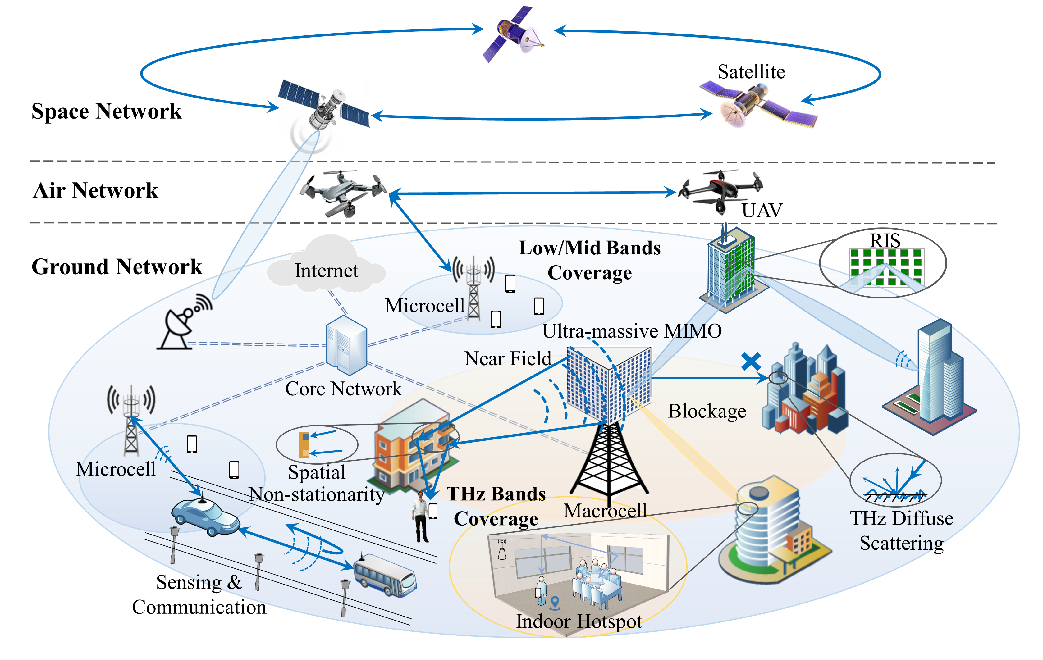
Figure 1: Application sceanrios and channel characteristics of 6G.

I-B1 Higher frequency band

Higher frequency band has large amounts of unallocated bandwidth. For example, THz wave (0.1–10 THz) has tens of GHz bandwidth spectrum resources near 300 GHz, due to the appropriate atmospheric transmission window. THz communication is therefore a promising way to achieve the KPI of peak transmission rate in Tb/s [12]. Moreover, THz communication can achieve functions such as expanded coverage and beam alignment by combining MIMO, JCAS and other technologies [14]. Because the millimeter wavelength of the THz band brings the possibility of large-scale antenna embedding within a few square millimeters and precise sensing at the centimeter level. However, no standardized THz channel model is available. The frequency supported by the ITU-R M.2412 channel model is up to 100 GHz. An accurate and low-complexity THz channel model should properly consider the propagation characteristics of THz waves, such as severe free space propagation loss, molecular absorption loss and sparsity. In addition, as the frequency increases, the Ralyleigh distance expands, and the THz communication system may operate in the near field, near-field effect also need to be considered in channel modeling. Therefore, in-depth knowledge of THz channel through measurement, modeling and simulation is a prerequisite for deploying THz wireless communication systems, which help to compensate or even take advantage of the characteristics of THz communication, such as strong signal attenuation, susceptibility to occlusion, and close coverage distance.

I-B2 Extremely large antenna array

Higher spectral efficiency and energy efficiency can be achieved by deploying extremely large antenna arrays in massive MIMO [15]. With the increase of integration, the scale of antenna array is expected to be further increased. The spatial resolution of Massive MIMO will be improved to enable fast beam alignment and real-time tracking. Nevertheless, near-field effects and spatial non-stationary characteristics will be more obvious in massive MIMO channel. Different from the assumptions of traditional MIMO channel. Near-field effects can range up to several hundred meters. The plane wave hypothesis is no longer valid when the propagation distance is less than the Rayleigh distance (in the near-field range). The physical mechanism of spatial non-stationarity is the difference of the visible cluster of antenna elements, which is another fundamental characteristic in massive MIMO channel. Hence, near-field effects and spatial non-stationary characteristics need to be studied through channel measurement and channel simulation, and included in channel modeling and channel simulation.

I-B3 New technology combinations

By combining other non-communications technologies, such as radar sensing and metamaterial RIS, the capabilities of the 6G communication system can be expanded. JCAS can achieve synergy between communication and sensing based on the sharing of hardware and software [16]. The predecessor of JCAS is recognized to be the idea of embedding communication signals into radar-sensing waveforms proposed by R. M. Mealy in 1963 [17]. Although JCAS is expected to reconstruct the environment and channel to meet the intelligence of 6G system [18], JCAS channel research needs to consider the characteristics and utilization of sensing signals. No traditional channel model can describe the algorithm design and performance evaluation of sensing, which strongly depends on the location of the target, transceiver, and scatterers [19].

RIS is an electromagnetic surface composed of a large number of programmable reflective elements. The physical properties of programmable reflection elements can be altered to actively regulate radiation characteristics [20]. The concept of programmable metamaterial is first proposed in 2014 [21]. RIS can significantly improve channel gain [5] by actively controlling the radio propagation environment. Moreover, RIS has the characteristics of low cost and high energy efficiency. Thus, RIS is considered a promising technology for 6G system. Nevertheless, RIS controls part of the reflection of radio waves, so the role of RIS should be taken into account in channel research. There is still a lack of mature techniques for accurate modeling and estimation of the surface and the channel, especially in the near-field range [5].

I-B4 More diverse scenarios

The 6G network is likely to be an architecture that integrates satellite systems, aerial networks, ground communications, sea communications, and underwater systems. With the rapid expansion of human activities in space, the need for satellite communication will become more common. However, current wireless communication networks have limited coverage as reported in [12]. It can only serve 70 percent of humanity, and covers only about 20 percent of the land mass, less than 6 percent of the earth’s surface. Universal coverage of the network benefits a variety of practical services and applications, but it will lead to more diverse communication scenarios. The channel of space-air-ground integrated network have the characteristics of long propagation distance and high node mobility [22]. Besides, when combined with technologies such as THz, ultra-massive MIMO, JCAS, and RIS, some propagation mechanisms become important, such as molecular absorption, reflection and scattering from rough surfaces, and the use of known/controllable environmental information also needs to be considered. For that reason, the number of typical communication scenarios will multiply, demanding for more channel measurement campaigns, channel models and channel simulation.

I-C Paper Contributions and Organization

So far, some research on 6G channels, including research surveys [7, 12, 23, 24] have been published. Nevertheless, there has not been a comprehensive survey paper on the whole 6G channel research. At the same time, 6G channel standardization work has been carried out, the 44th meeting of ITU-R Working Party 5D will determine the 6G vision, and start 6G technology assessment. However, no 6G channel simulation platform is available. This paper aims to fill the research gap in survey and simulation of 6G channel. A survey and tutorial focusing on promising 6G key technologies is given. Specific contributions are as follows:

• The state-of-the-art standard channel model for 5G systems, ITU-R M. 2412 [25] and 3GPP TR 38.901 [26], is introduced. And the challenges of 6G channel research are summarized, including higher frequencies, larger antenna arrays, more complex propagation mechanisms, and more diverse scenarios.

• A review on channel measurement and modeling is presented for four promising and urgent tehcnologies in 6G: THz, massive MIMO, JCAS, and RIS. And the future research directions are prospected from the aspects of channel measurement, characteristic modeling, and modeling method, respectively.

• The first 6G channel simulation platform, BUPTCMG-IMT2030, is introduced. The platform framework and simulation steps are detailed. The simulation examples of THz, spatial non-stationarity, and RIS are given.

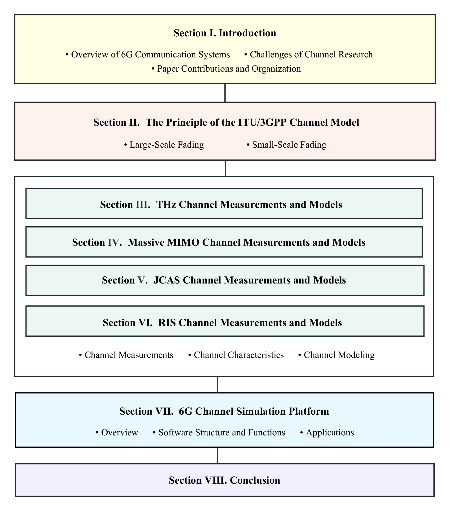
Figure 2: The organization of the paper.

The rest of this article is organized as shown in Fig. 2. In Section II, the 5G standard channel modeling principles are outlined, followed by a discussion of the challenges of 6G channel modeling. Sections III through VI provide an overview of the current state of research on THz, massive MIMO, JCAS, and RIS channel models in terms of measurement and modeling, then the prospects are discussed, respectively. Section VII presents an overview of the developed 6G channel simulation platform BUPTCMG-IMT2030. Finally, conclusions are drawn in Section VIII.

II The Principle of the ITU/3GPP Channel Model

In this section, we briefly introduce the channel model modeling principles of ITU-R M.2412 [25] and 3GPP TR 38.901 [26], including large-scale fading path loss modeling (Floating-intercept (FI) model, Close-in (CI) model, and Alpha-Beta-Gamma (ABG) model) and small-scale fading modeling of 3D MIMO. Given that the primary module is the core module, and support the evaluation of all 5G technologies.

II-A Modeling principles for large-scale fading

The large-scale fading models are crucial to deciding the coverage. In the ITU-R M.2412 [25] and 3GPP TR 38.901 [26] channel model, the large-scale fading channel models can be classified into three types: the CI model, FI model, ABG model [27, 28, 29]. The FI model is widely used. It is expressed as follows:

$$PL_{FI}(d)=\beta_{FI}+10\alpha_{FI}\textrm{log}_{10}d+X_{\sigma}^{FI},$$ (1)

where $\beta_{FI}$ and $\alpha_{FI}$ are two parameters of fit and $X_{\sigma}^{FI}$ is a zero-mean Gaussian variable representing the shadowing. Note that $\beta_{FI}$ is frequency dependent. This model has been adopted in channel standardizations due to its simplicity, although it does not consider the frequency dependence. The ABG model is represented as [28] [30]:

$$\begin{split}PL_{ABG}(f,d)[\textrm{dB}]=&10\alpha_{ABG}\textrm{log}_{10}(\frac{d}{d_{0}})+\\ &\beta_{ABG}+10\gamma_{ABG}\textrm{log}_{10}(\frac{f}{1\ \textrm{GHz}})+X_{\sigma}^{ABG},\end{split}$$ (2)

where $d_{0}$ is the received-power reference point, which is typically chosen to be 1m, $\alpha_{ABG}$ and $\gamma_{ABG}$ are the distance and frequency dependence on path loss respectively. The typical value of $\gamma_{ABG}$ is 2, which corresponds to free space propagation. In this ABG model, we can see that path loss varies with the frequency and the spatial distance. CI free space reference distance path loss model is also a function of frequency. In [31], it was investigated that CI and ABG models were evaluated to offer comparable modeling performance using real data. The CI model can be written as

$$\begin{split}PL_{CI}(f,d)[\textrm{dB}]=&20\textrm{log}_{10}(\frac{4\pi d_{0}f}{c})+10\alpha_{CI}\textrm{log}_{10}(\frac{d}{d_{0}})+X_{\sigma}^{CI}\\ &\textrm{for}\ d\geq d_{0},d_{0}=1m.\end{split}$$ (3)

II-B Modeling principles for small-scale fading

3D MIMO is one of the most important technologies for 5G. A diagram of the 3D MIMO channel model is shown in Fig. 3. The small sphere with several dots inside represents a scattering region causing one cluster. Each cluster is constituted by $M$ rays, and $N$ clusters are assumed. Tx and Rx are amounted with $S$ and $U$ antennas antennas. The small scale parameters (SSPs) like delay $\tau_{n,m}$, the azimuth angle of arrival $\phi_{rx,n,m}$, the elevation angle of arrival $\theta_{rx,n,m}$, the azimuth angle of departure $\phi_{tx,n,m}$ and the elevation angle of departure $\theta_{tx,n,m}$ are assumed to be different for each ray. We can see that radio waves propagate in the 3D space, and MPCs have not only horizontal characteristics but also vertical characteristics.

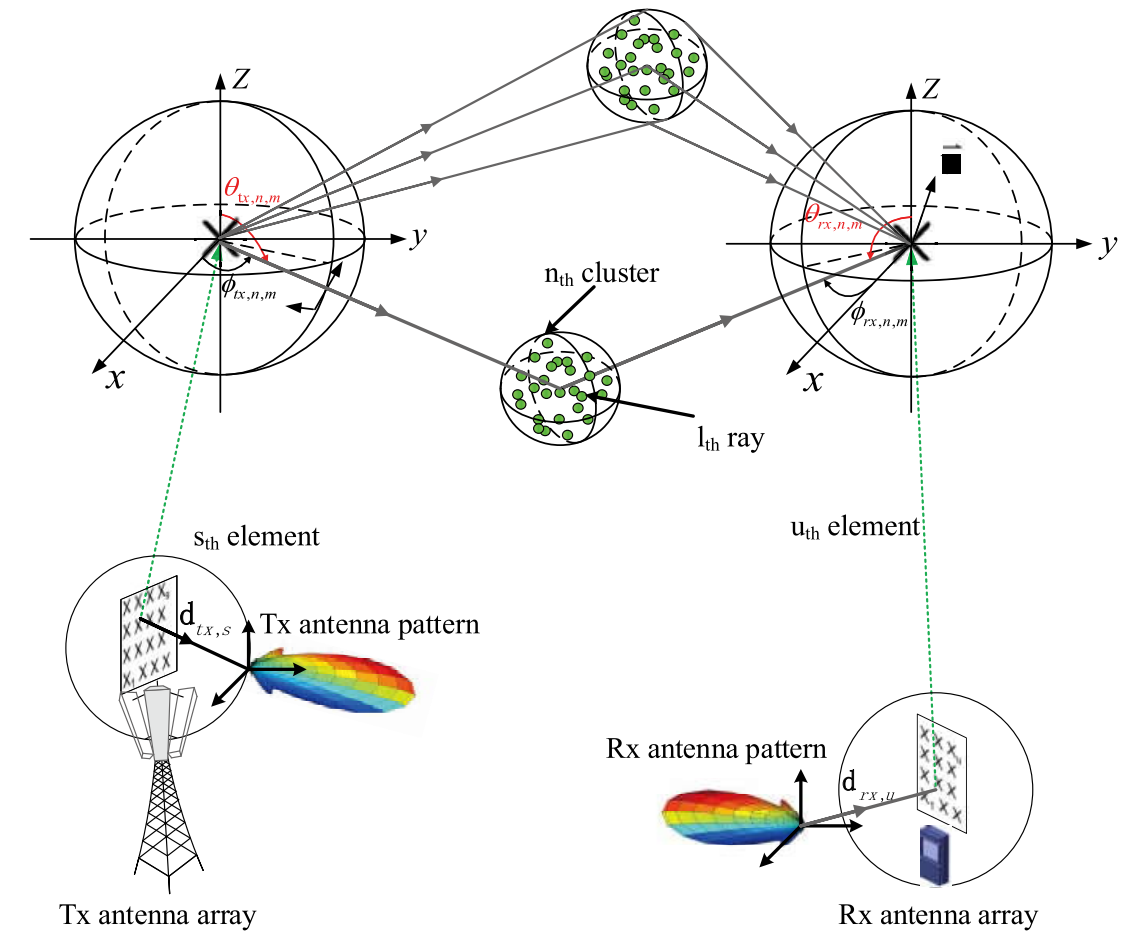
Figure 3: The diagram of ITU-R 5G channel model [32].

In the ITU-R 5G channel model, the channel impulse response (CIR) for the $s$th transmitter antenna, and the $u$th receiver antenna and the $n$th cluster should be given by

$$\begin{split}&h_{u,s,n}(t,\tau,\bm{\Omega},\bm{\Psi})=\sum_{m=1}^{M_{n}}a_{n,m}G_{s}(\bm{\Psi}_{n,m})G_{u}(\bm{\Omega}_{n,m})\\ &\textrm{exp}(j2\pi\lambda^{-1}(\vec{r}_{R,n,m}\cdot\vec{d}_{R,u}))\textrm{exp}(j2\pi\lambda^{-1}(\vec{r}_{T,n,m}\cdot\vec{d}_{T,s}))\\ &\delta(\tau-\tau_{n,m})\delta(\bm{\Omega}-\bm{\Omega}_{n,m})\delta(\bm{\Psi}-\bm{\Psi}_{n,m})\end{split}$$ (4)

where $\bm{\Omega_{n,m}}$ and $\bm{\Psi_{n,m}}$ should include both azimuth angle and elevation angle for 3D MIMO systems as follows

$$\begin{split}&\bm{\Omega_{n,m}}=(\phi_{R,n,m},\theta_{R,n,m}),\\ &\bm{\Psi_{n,m}}=(\phi_{T,n,m},\theta_{T,n,m}),\end{split}$$ (5)

where $\phi_{R,n,m}$ and $\theta_{T,n,m}$ represent the azimuth angle and the elevation angle of the $m$th MPC within the $n$ cluster at the RX side and the TX side, respectively. In practical systems, antennas have specific patterns to reinforce system performance. And slant polarized antennas are used. Thus, the antenna patterns must be modelled when generating the CIR. Horizontal and vertical (linear polarization) or $+45^{\circ}/-45^{\circ}$ (slant polarization) are examples of orthogonal polarizations [33]. Given that dual polarization is utilized, Equ. (4) should be changed to Equ. (6).

$$\begin{split}H^{NLOS}_{u,s,n}(t,\tau)=\sqrt{\frac{P_{n}}{M}}\sum_{m=1}^{M}\begin{bmatrix}F_{rx,u,\theta}(\theta_{n,m,EOA},\phi_{n,m,AOA})\\ F_{rx,u,\phi}(\theta_{n,m,EOA},\phi_{n,m,AOA})\end{bmatrix}^{T}\begin{bmatrix}\textrm{exp}(j\Phi_{n,m}^{\theta\theta})&\sqrt{\kappa_{n,m}^{-1}}\textrm{exp}(j\Phi_{n,m}^{\theta\phi})\\ \sqrt{\kappa_{n,m}^{-1}}\textrm{exp}(j\Phi_{n,m}^{\phi\theta})&\textrm{exp}(j\Phi_{n,m}^{\phi\phi})\end{bmatrix}\\ \begin{bmatrix}F_{tx,s,\theta}(\theta_{n,m,EOD},\phi_{n,m,AOD})\\ F_{tx,s,\phi}(\theta_{n,m,EOD},\phi_{n,m,AOD})\end{bmatrix}\textrm{exp}(j2\pi\frac{r_{rx,n,m}^{T}\cdot d_{rx,u}}{\lambda_{0}})\textrm{exp}(j2\pi\frac{r_{tx,n,m}^{T}\cdot d_{tx,s}}{\lambda_{0}})\textrm{exp}(j2\pi v_{n,m}t)\delta(\tau-\tau_{n,m})\end{split}$$ (6)

In Equ. (6), $\left\{{\Phi}_{n,m}^{\theta\theta},{\Phi}_{n,m}^{\theta\phi},{\Phi}_{n,m}^{\phi\theta},{\Phi}_{n,m}^{\phi\phi}\right\}$ are random initial phase for each ray $m$ of each cluster $n$ and for four different polarisation combinations ($\theta\theta$, $\theta\phi$, $\phi\theta$, $\phi\phi$). The distribution for initial phases is uniform within ($-\pi,\pi$). ${F}_{rx,u,\theta}$ and ${F}_{rx,u,\phi}$ are the field patterns of receive antenna element $u$ in the direction of the spherical basis vectors, $\theta$ and $\phi$ respectively, ${F}_{tx,s,\theta}$ and ${F}_{tx,s,\phi}$ are the field patterns of transmit antenna element $s$ in the direction of the spherical basis vectors, $\theta$ and $\phi$ respectively. $r_{rx,n,m}$ is the spherical unit vector with AOA ${\phi}_{n,m,AOA}$ and elevation of arrival (EOA) ${\theta}_{n,m,EOA}$, while $r_{tx,n,m}$ is the spherical unit vector with AOD ${\phi}_{n,m,AOD}$ and elevation of departure (EOD) ${\theta}_{n,m,EOD}$. $d_{rx,u}$ and $d_{tx,s}$ are the location vectors of receive antenna element $u$ and transmit antenna element $s$, respectively. $\kappa_{n,m}$ is the cross polarisation power ratio in linear scale. $\lambda_{0}$ is the wave length of the carrier frequency. $v_{n,m}$ is the Doppler frequency component of ray $n,m$. $P_{n}$ is the normalized power of the $n$th cluster. The superscript “NLOS” denotes that Equ. (6) describes the CIR in the non-line-of-sight (NLOS) case.

For a LOS scenario, the CIR consists of two parts, i.e., deterministic component (usually the LOS path) and random components (often called scattered components). Also, two polarization vectors are assumed to be orthogonal exactly. Thus, the LOS path can be written as Equ. (7). $\textrm{exp}(j\Phi_{LOS})$ is the initial phase of the LOS path. It can be either random or computed according to $\Phi_{\textrm{LOS}}=-2\pi\frac{d_{3D}}{\lambda_{0}}$, where $d_{3D}$ is the distance between TX and RX in the 3D space.

$$\begin{split}H^{LOS}_{u,s,1}(t)=\begin{bmatrix}F_{rx,u,\theta}(\theta_{LOS,EOA},\phi_{LOS,AOA})\\ F_{rx,u,\phi}(\theta_{LOS,EOA},\phi_{LOS,AOA})\end{bmatrix}^{T}\begin{bmatrix}1&0\\ 0&-1\end{bmatrix}\begin{bmatrix}F_{tx,s,\theta}(\theta_{LOS,EOD},\phi_{LOS,AOD})\\ F_{tx,s,\phi}(\theta_{LOS,EOD},\phi_{LOS,AOD})\end{bmatrix}\\ \textrm{exp}(j\Phi_{LOS})\textrm{exp}(j2\pi\frac{r_{rx,LOS}^{T}\cdot d_{rx,u}}{\lambda_{0}})\textrm{exp}(j2\pi\frac{r_{tx,LOS}^{T}\cdot d_{tx,s}}{\lambda_{0}})\textrm{exp}(j2\pi v_{LOS}t).\end{split}$$ (7)

In addition, K-factor is used to describe the CIR in the LOS scenario. K-factor is defined as the power ratio of the deterministic component to that of the other stochastic components [34]. It can be a measure of small scale variations in time, space, or frequency, i.e., temporal, spatial, or spectral selectivity [35]. Thus, through adding the LOS channel coefficient to the NLOS channel CIR and scaling both terms according to the desired K-factor $K$, the CIR in the LOS scenario can be written as

$$\begin{split}H_{u,s}^{LOS}(t,\tau)=&\sqrt{\frac{1}{K+1}}\sum_{n=1}^{N}H_{u,s,n}^{NLOS}(t,\tau)+\\ &\sqrt{\frac{K}{K+1}}H^{LOS}_{u,s,1}(t)\delta(\tau-\tau_{LOS}).\end{split}$$ (8)

This model assumes that the LOS path appears in the first cluster. It reflects the actual propagation phenomenon in channels and can describe the channel correctly.

To get a complete mathematical expression of channels, the large scale fading channel model and the small scale fading channel model should be combined by applying path loss and shadowing for the channel coefficients $H$.

III THz Channel Measurements and Models

To increase the data rate 100 to 1000 times faster than 5G, 6G will use a higher frequency spectrum than previous generations [12]. Among the candidates, THz frequency bands have been identified as a promising option due to their wide bandwidth and low interference characteristics. Europe, the United States, China, and other countries and regions have recognized the potential of the THz spectrum for communications. They have placed a high priority on its development and utilization. In addition, the ITU has shown strong support for research and development of THz communication technologies. As shown in Fig. 4, the ITU has allocated a total of 244.2 GHz in the 100-450 GHz frequency band for fixed services and land mobile applications. Specifically, the ITU has allocated 12 bands (total 1017.2 GHz bandwidth) within the 100-275 GHz frequency range [36]. It is noteworthy that the largest contiguous bandwidth available in any of the frequency bands is 23 GHz, and it is only at the upper band. Below 200 GHz, the largest contiguous bandwidth currently allocated for fixed or mobile use is 12.5 GHz. This limited availability of contiguous bandwidths poses a challenge for developing high-bandwidth wireless communication systems in 6G. Therefore, by the ITU Radio Regulations 2020, WRC-19 identified 275-296 GHz, 306-313 GHz, 318-333 GHz, and 356-450 GHz, for a total of 139 GHz that can be used for fixed service and land mobile applications [37]. And the maximum available continuous bandwidth reaches 94 GHz.

In addition, spectrum planning and allocation regulators in different countries and regions have released parts of the THz band to facilitate scientific research. For example, the Federal Communications Commission (FCC) decision in March 2019 authorized the unlicensed use of 116-123 GHz, 174.8-182 GHz, 185-190 GHz, and 244-246 GHz in the United States [38]. Japan’s Ministry of Information and Communication (MIC) designated the frequency range of 116-134 GHz as ”Commercial Telecommunications Services” in 2015 [39], and the 152-164 GHz and 287.5-312.5 GHz bands were made available for experimental testing in 2020 [40]. In 2018, the European Conference of Postal and Telecommunications Administrations (CEPT) and the European Radiocommunications Committee (ERC) released a recommendation on ”Short Range Devices,” also known as ”unlicensed devices,” which specified provisions for these devices to operate within the frequency ranges of 122-122.25 GHz and 244-246 GHz [41]. The allocation of spectrum for 6G THz communications is a topic under discussion, and the next scheduled consideration is at the WRC-23 meeting. However, a definitive decision on the matter is not expected until the subsequent WRC-27 [42].

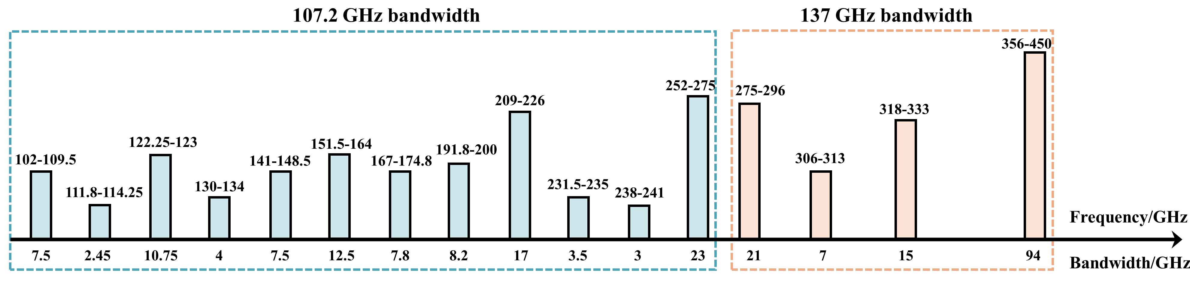
Figure 4: Available bandwidths from 100 to 450 GHz for 6G.

III-A THz Channel Measurements

Many research organizations and institutions conduct a large number of THz channel measurement campaigns in the above-mentioned frequency bands. We classify and summarize the channel measurement campaigns by frequency band, as shown in Table I. In the 100-275 GHz sub-THz band, it is generally concerned with several frequency points 100, 140, 158, and 205 GHz [13] [14] [43, 44, 45, 46, 47, 48, 49, 50, 51, 52, 53, 54, 55, 56, 57, 58, 59, 60, 61, 62, 63, 64, 65, 66, 67, 68, 69, 70, 71]. And in the 275-450 GHz THz band allocated by WRC-19 for fixed services and land mobile applications, more measurement campaigns are conducted in 300 and 360 GHz frequency bands [72, 73, 74, 75, 76, 77, 78, 79, 80, 81, 82, 83, 84, 85, 86, 87, 88, 89, 90, 91, 92, 93, 94, 95, 96, 97]. However, in the 450-1100 GHz band [93] [98, 99, 100], there are fewer channel measurement campaigns limited by hardware capabilities such as instruments and equipment.

Most channel sounders widely used in THz channel measurement campaigns are the frequency domain vector network analyzer (VNA)-based sounders [101]. Due to the high loss of the cable, the measurement distance is usually not far and can be extended up to 100 m by radio-over-fiber (RoF) [14]. The correlation-based time-domain channel sounders have also been used in a number of THz channel measurements. Since the transmitter and receiver are independent of each other and do not need cable connections, the correlation-based time-domain channel sounders are preferable for measurements in outdoor environments [43]. In addition, the THz time-domain spectroscopy system (THz-TDS) [102] based channel sounders are limited by the output power and are commonly used for measurements of reflection and diffraction properties of materials.

The THz band channel measurements focus on desktop, meeting room, office, data center, computer motherboard, outdoor street, and indoor factory scenarios, covering the vision scenarios of THzCom, such as wireless local area networks (WLAN), wireless personal area networks (WPAN), data center network (DCN), and intra-device communication (IDC) [103]. However, the wireless backhaul/fronthaul scenario has been poorly studied [104]. And most of the channel measurement campaigns in these scenarios are in the 100-450 GHz frequency bands. Furthermore, the researches include the channel propagation mechanism, and the channel statistical characteristics of the ITU standard models [26] of the THz bands, which will be described in detail in the next section.

TABLE I: Summary of THz channel measurement campaigns

Frequency /BW (GHz)	Sounder	Scenario	Channel characteristics	Reference
100 - 275 GHz
100/6	VNA+RoF	Empty room	spatial non-stationarity	[14]
120/40	VNA	Computer motherboard	PL, DS, reflection/penetration loss	[51]
135/10		Data center	PL, SF, DS, AS, cluster numbers, intra/inter-cluster parameters	[50]
140/60		Indoor	PL; SF; DS;	[44]
142/1	Correlation- based	Office, conference, classrooms, hallways, factory building	PL, SF, DS, AS, cluster numbers, intra/inter-cluster parameters	[63, 64]
		Building materials	Reflection, transmission, PL, SF, XPD	[65]
		UMi	PL, foliage attenuation, spatial consistency,coverage	[66, 67, 68, 69]
143.1/4	VNA+RoF	Shopping mall, airport check-in hall	PADP, PDP, PAS, PL, DS, AS	[52, 53]
144.75/7.5 145.5/1 140.5/1		Outdoor(courtyard, crossroad, canyon)	PDP, PL, SF, DS, AS, Power distribution of MPC, Qtapnumber	[55, 56] [58, 60]
[220:10:330]/2	Correlation- based	Desktop	PL, celluar performance, reflection	[43, 13]
220-330	VNA+RoF	Hall	PDP, PL, DS, AS, PADP	[105]
205/8	VNA	Indoor(meeting room, office room)	PL, SF, DS, AS, K, cluster numbers, intra/inter-cluster parameters	[48]
275 - 450 GHz
280/120	VNA	Download kiosk	K, RMS DS	[88]
300/2	Correlation- based	UMi (courtyard)	PDP, PL, DS, AS	[94, 96]
300/2	VNA+RoF	Spacious hall	PDP	[14]
304.2/8	Correlation- based	V2V	Blockage, PDP, PL, RMS DS, AS	[84]
305/10	VNA	Desktop, building material	PL, absorption coefficients	[83]
310/20		Desktop	PDP, PL, SF, RMS DS, TCF	[73]
		Computer motherboard	PL, SF, reflection	[74]
		Data center	PL, reflection	[74]
313.5/15		Indoor(hallway, corridor)	PL, SF, DS, AS, K, cluster numbers, intra/inter-cluster parameters	[79, 80]
		Outdoor(campus street, atrium)		[81, 82]
450 - 1100 GHz
450/500	THz-TDS	Building material	Diffuse scattering	[93]
625/250	VNA	Desktop	Atmospheric effects; PDP	[100]
925/350		Building material	Penetration losses	[99]
1000/200		Desktop	Ground reflections	[98]
UMi: urban microcell, V2V: vehicle-to-vehicle, PDP: power delay profile, PL: path loss, SF: shadow fading, K: Rician K fator, RMS: root mean square, DS: delay spread, AS: angular spread, XPD: cross-polarization discrimination, TCF: temporal correlation function, InF: indoor factory.

III-B THz Propagation and Channel Characteristics

The THz characteristics research can be roughly categorized into two kinds [14]. The first kind focuses on the effect of different materials or obstacles on the THz propagation mechanisms such as reflection and scattering [106]. The second kind is dedicated to the traditional channel characteristics of the ITU standard models and new channel characteristics in THz bands, such as sparsity, non-stationary in frequency and spatial domains. Moreover, the research of propagation mechanism characteristics is the key foundation and fundamental premise for THz channel characteristics research.

III-B1 THz propagation characteristics

The propagation of THz waves primarily involves line-of-sight (LoS) communication, which is attributed to the higher path loss experienced [107]. However, it is noteworthy that NLoS propagation may also occur in certain cases. The reflection, scattering, transmission, and diffraction at NLoS are fundamental propagation mechanisms that should be thoroughly characterized in order to establish possible THz wireless links. The attenuation is high enough to neglect transmission [108, 109] as a relevant propagation mechanism in the THz band. And the diffraction does not contribute significantly to the received power already at mm-waves (see investigations at 60 GHz [110]). Therefore, this subsection analyzes and models the reflection and scattering propagation characteristics of THz waves.

$\bullet$ Reflection characteristics

At THz bands, the characteristics of the reflection in case of ideally smooth and homogeneous surfaces can be described by the well-known Fresnel reflection coefficient $\Gamma$ [111]. The Fresnel reflection coefficient expressions for perpendicular ($\Gamma_{{\rm{TE}}}$) and parallel ($\Gamma_{{\rm{TM}}}$) polarizations for such smooth surfaces are expressed as

$${\Gamma_{{\rm{TE}}}}=\frac{{Z\cos{\theta_{i}}-{Z_{0}}\cos{\theta_{t}}}}{{Z\cos{\theta_{i}}+{Z_{0}}\cos{\theta_{t}}}},$$ (9)

and

$${\Gamma_{{\rm{TM}}}}=\frac{{Z\cos{\theta_{t}}-{Z_{0}}\cos{\theta_{i}}}}{{Z\cos{\theta_{t}}+{Z_{0}}\cos{\theta_{i}}}},$$ (10)

here, $\theta_{i}$ is the incident angle, $\theta_{t}$ is the reflection angle, ${Z_{0}}=377\enspace{\rm{}}\Omega$ denotes the free space impedance, and $Z$ is the wave impedance of the reflected material, calculated as

$$Z=\sqrt{\frac{{{\mu_{0}}}}{{{\varepsilon_{0}}({n^{2}}-{{(\frac{{\alpha c}}{{4\pi f}})}^{2}}-j\frac{{2n\alpha c}}{{4\pi f}})}}},$$ (11)

where $\mu_{0}$, $\varepsilon_{0}$, $c$, and $f$ are the free space permeability, permittivity, velocity, and frequency of the incident wave, respectively. $n$ is the complex refractive index of the smooth surface and $\alpha$ is the absorption coefficient of the incident surface material.

At lower frequencies, the surface of the material is considered primarily as a smooth surface. However, as the frequency increases to the sub-THz band, the wavelength is short enough to be very close to the surface roughness of typical materials. Therefore, in the THz band, the material cannot be considered as a smooth surface. For the reflection coefficient of a rough surface, generally a Rayleigh model based on the Kirchhoff-approximation is modified. In this method, the modified reflection coefficient is obtained by introducing a roughness factor $\rho$. The Rayleigh roughness factor can be expressed as [112]

$$\rho=\exp(-\frac{1}{2}{(4\pi{\sigma_{h}}\frac{{\cos{\theta_{i}}}}{\lambda})^{2}}),$$ (12)

where, $\sigma_{h}$ denotes the standard deviation height of the material surface roughness, and $\lambda$ indicates the wavelength of the incident wave. Then, the modified reflection coefficient $\Gamma^{\prime}$ is expressed as

$$\Gamma^{\prime}=\rho\Gamma.$$ (13)

It is observed that this reflection coefficient model is a function of frequency and angle of incidence, and reference [43] verifies this phenomenon based on experiments. As a representative, the results of the plasterboard are shown in Fig. 5. The points of measured data fit well with the reflection coefficient model. As observed the reflection coefficient of the material and its growth rate increase with the increase of the angle of incidence. Therefore, the model characterizes the reflection coefficient as a function of frequency and angle of incidence. In addition, it shows a low root-mean-square error with the measured data.

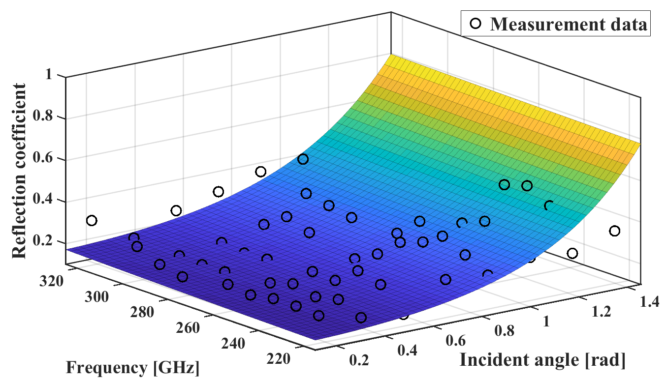
Figure 5: The reflection coefficients measurement data and fitting results of plasterboard from 220 to 320 GHz.

$\bullet$ Scattering characteristics

In the conventional microwave band, scattering plays a very weak role compared to direct and reflected radiation. However, in the THz band, higher frequencies mean that wavelengths will likely be smaller than the surface roughness of many objects, and surfaces that would otherwise be considered smooth will be considered rough [113]. The Rayleigh criterion [114] is commonly used to determine whether a surface is rough or not. Therefore, the major challenges at THz frequencies are the modeling of the most significant propagation phenomenon of diffuse scattering, by which an incident ray may split into specular and several non-specular rays after bouncing off from rough materials. Notice that the scattering problem of electromagnetic waves is still not solved completely and no exact closed-form solutions exist yet. However, numerous approximate methods have been developed for wave scattering at rough surfaces in order to predict and interpret experimental data. Amongst these, there are two main types of diffuse scattering models, the effective roughness (ER) model [115] and Beckmann-Kirchhoff (B-K) model [116], which originate from the field of optical propagation, and the radar cross section (RCS) model [117].

The Lambertian model, Directive model, and Backscattering Lobe model evolved from the ER model can effectively describe the scattering patterns on the surfaces of materials with different roughness and are widely used in the current diffuse scattering propagation research. The three models are not described in detail here. For a complete derivation, the inclined reader is referred to [118] and [109].

Compared to numerical approaches [119], the Kirchhoff model offers a higher computational efficiency and can easily be implemented into a ray tracing algorithm. In reference [120], the indoor multipath propagation and its impact on massive MIMO channels considering smooth and rough surfaces are investigated by employing the B-K model. The Kirchhoff approach is verified by an experimental study of diffuse scattering from randomly rough surfaces commonly encountered in indoor environments using a fiber-coupled THz time-domain spectroscopy system to perform angle- and frequency-dependent measurements in [93].

The RCS model is a measure of the power density scattered in the direction of the receiver relative to the power density of the radio wave illuminating the scattering object. It can be thought of as a combination of contributions from small-scale and large-scale roughness, and the surface scattering can be calculated by dividing the surface into small-scale and large-scale patches [109]. Thus,

$$\operatorname{RCS}\sigma=\sigma_{\text{rough }}+\left|\chi_{s}^{2}\right|\sigma_{\text{smooth }},$$ (14)

with $\sigma_{\text{rough }}$ and $\sigma_{\text{smooth }}$ as small-scale and large-scale RCS $\sigma$, respectively. The weighting factor $\chi_{s}$ is the rough surface height characteristic function. This factor is given as $\chi_{s}=\exp\left(-k_{0}^{2}\cdot\sigma_{h}^{2}\cos^{2}\theta_{i}\right)$ and approaches to 1 as frequency decreases, which implies that $\sigma_{\text{smooth }}$ dominates the RCS $\sigma$. However, as frequency reaches to THz range, $\chi_{s}$ becomes negligible for rough surfaces, and the impact of $\sigma_{\text{rough }}$ becomes much more significant. Reference [109] compares the backscattered power for certain materials at 100 GHz and 1 THz using the RCS model. Since the RCS model is an empirical-based model, the RCS model can be better parameterized to predict the accurate scattered power based on the field measurements for various materials having different surface roughness and permittivity at different frequencies.

III-B2 THz Channel Characteristics

The signals transmitted over THz channels experience characteristics that are different from those encountered at lower frequencies, which results in new and pressing challenges [121]. Some of the THz band characteristics are described as follows: i) High propagation loss: In wireless propagation, the spreading loss increases quadratically with frequency. Given the very high frequencies at the THz band, the signal propagated over a THz link is impacted by the severe spreading loss [13]. ii) Molecular absorption loss: The THz band is uniquely characterized by the molecular absorption loss, resulting from the phenomenon that THz signal energies are absorbed by water vapor and oxygen molecules in the propagation medium [122]. In particular, certain frequencies of the THz spectrum are very sensitive to molecular absorption, where the THz signal energy is profoundly decreased [43]. iii) Less number of multipath components: The wavelength of THz signals is extremely short, thus becoming comparable to the surface roughness of typical objects in the environment [123]. This implies that the surfaces considered smooth at lower frequencies are rough at the THz band. When THz waves hit such rough surfaces, very high reflection, diffraction, and scattering losses occur, leading to significant attenuation of the number of NLoS multipath components.

The channel characteristics of high propagation loss and molecular absorption loss can be characterized by path loss. Whereas, a less number of multipath components require a novel method to characterize and model them.

$\bullet$ Path loss characteristics

The modeling of path loss and shadow fading in the THz band follows the 5G modeling methods, such as the FI model, ABG model, and CI model shown in equations 1, 2, and 3. Based on the references in Table I, the path loss exponent for indoor and outdoor scenarios using the CI model is summarized, as shown in Fig. 6. Firstly, it is shown that the path loss exponent of the THz band is close to 2 in most cases, especially in the LoS scenarios. Secondly, there is no obvious difference in the PLEs between indoor and outdoor scenarios. Thirdly, the PLEs of NLoS scenarios are remarkably higher than that of the LoS scenario. It is due to the blocking losses caused by walls, cars, etc. can be as large as tens of dB in the NLoS scenarios, which means that severe attenuation can occur. Finally, the PLEs remain largely different at the same frequency band even in similar scenarios. It is caused by the large differences in the measurement environment, and the inconsistency of the measurement platform and the data processing methods.

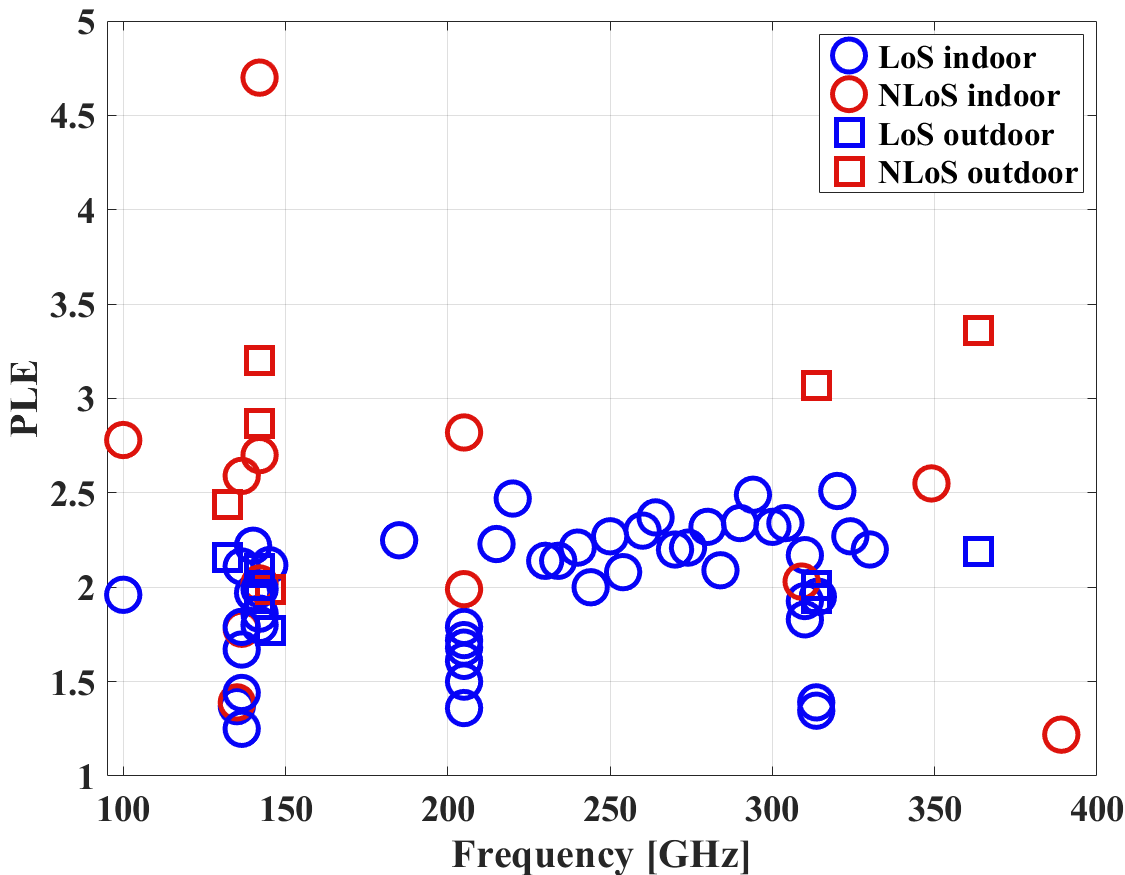
Figure 6: The representative results of path loss exponent based on measurements of THz channels.

Due to the wider span of the THz band, it will show a stronger frequency dependence. To further investigate the frequency dependence of path loss in THz bands, [13] uses the ABG model to fit the measured path loss. The measured path loss and the ABG model are plotted shown in Fig. 7 and the derived parameters are presented in equation 15. It denotes that the frequency dependence is a little stronger than that in the free space [121].

$$\begin{split}\mathrm{PL}_{\mathrm{ABG}}(f,d)[\textrm{dB}]=&19.3\;\textrm{log}_{10}(\frac{d}{d_{0}})+\\ &13.27+21\;\textrm{log}_{10}(\frac{f}{1\ \textrm{GHz}})+X_{3.78}^{\rm{ABG}},\end{split}$$ (15)

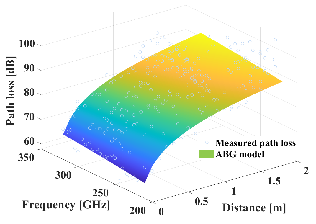
Figure 7: The multiple-frequencies measurement data and path loss modeling results from 220 to 330 GHz.

$\bullet$ Channel sparsity characteristics

In the THz band, the number of clusters is of general interest. A cluster is a group of multipath components that arrive at the receiver within a short time interval and with similar angles of arrival. Clusters are typically caused by the reflection or scattering of the signal from a single object in the environment, such as a building or a tree [124].

Several pieces of researches have been carried out for channel sparsity, in which the sparsity of THz channels can be observed qualitatively by the number of clusters. As shown in Fig. 8, the cluster number results of indoor and outdoor for LoS and NLoS scenarios in the literature are given. It can be observed that in the THz band, the number of clusters is concentrated between 2 and 6, which is significantly smaller than the 15/19 clusters in the 3GPP standard, indicating the possible sparsity of the THz channel. In addition, the number of clusters in the outdoor scenario is slightly smaller than that in the indoor scenario, which is mainly because the indoor environment is richer in scatterers and has more multipath components [125].

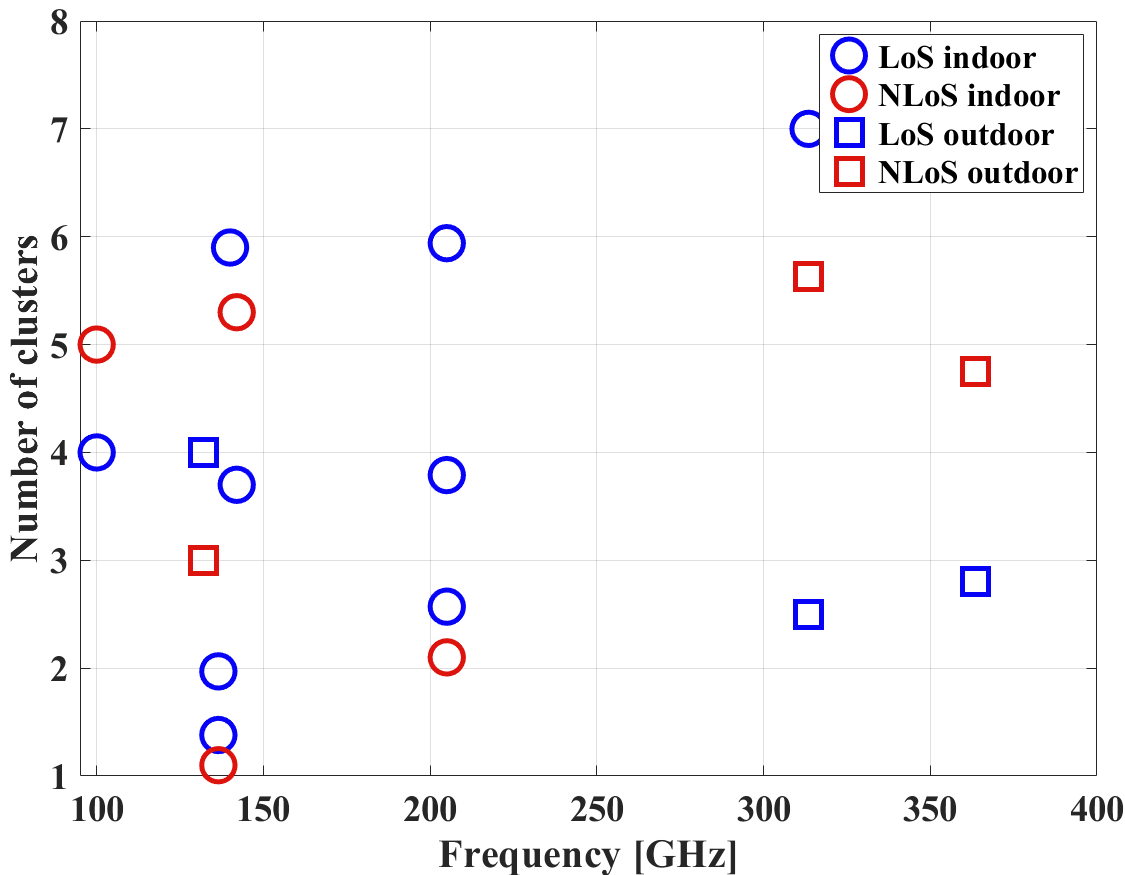
Figure 8: The representative results of number of clusters based on measurements of THz channels.

We roughly and qualitatively discover that the THz channel exhibits sparsity in terms of the number of clusters. However, a more fair and reasonable method to analyze and model this characteristic is necessary. The channel sparsity is analyzed and modeled in cmWave, mmWave, and sub-THz bands by multi-band measurements in reference [126]. The channel measurements at 6, 26, and 132 GHz were performed to analyze the channel sparsity by the Gini index, expressed as

$$G=1-2\sum_{i=1}^{R}\frac{p_{i}}{\|\mathbf{p}\|_{1}}\left(\frac{R-i+\frac{1}{2}}{R}\right),$$ (16)

where $R$ represents the number of rays, $p_{i}$ represents the power of the i-th ray. $\mathbf{p}$ represents a power vector composed of the power of $R$ rays. The elements in $\mathbf{p}$ are arranged in ascending order, i.e., $p_{1}<p_{2}<\cdots<p_{R}$. The subscripts are after sorting.

From the cumulative distribution function (CDF) curves of the Gini index generated by the measurement as illustrated in Fig. 9, the blue, black, and red lines represent the Gini index of cmWave, mmWave, and sub-THz channels, respectively. It is found that the sparsity of sub-THz channels is greater than that of the cmWave and mmWave channels, as shown by the Gini index of the sub-THz channel which is closer to 1. The dashed line represents the CDF curves of the Gini index derived from the simulation based on the 3GPP channel model [121]. It is found that the Gini index derived by the 3GPP channel model is much smaller than that calculated by the measurement. It proves that the 3GPP channel model is deficient in characterizing sparsity by the Gini index. In addition, the difference in channel sparsity between cmWave and mmWave channels is slight, which demonstrates that the 3GPP channel model cannot classify the sparsity characteristics of these frequency bands.

Therefore, the underlying framework of the 3GPP channel model needs to be corrected in the THz band. The intra-cluster power allocation model proposed uses the intra-cluster K-factor (ICK) to change the power distribution within the cluster. The channel coefficients of the n-th cluster can be expressed as

$$\begin{array}[]{c}H_{n}(t)=\sqrt{\frac{I}{I+1}\cdot P_{n}}\cdot c_{1}\exp\left(j2\pi v_{1}t\right)\\[14.22636pt] +\sqrt{\frac{1}{{I+1}}\cdot\frac{{{P_{n}}}}{{M-1}}}\sum\limits_{m=2}^{M}c_{m}\exp\left(j2\pi v_{m}t\right),\end{array}$$ (17)

where $P_{n}$ represents the power of the n-th cluster and $M$ represents the number of rays per cluster. $c_{m}$ is the complex channel coefficient. The coefficient includes the radiation pattern of the antennas, random phases, and path loss. $v_{m}$ is the doppler frequency. And the expression of ICK ($I$) is

$$I=\frac{\max\left(\mathbf{p}_{n}\right)}{\left\|\mathbf{p}_{n}\right\|_{1}-\max\left(\mathbf{p}_{n}\right)},$$ (18)

where $\mathbf{p}_{n}$ represents the vector composed of the power of all rays within the n-th cluster. The modified 3GPP channel model with the proposed intra-cluster power allocation model has the ability to characterize channel sparsity in the delay domain, which is verified by theoretical derivation and simulation experiments.

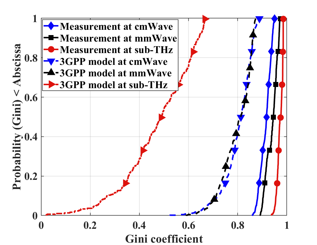
Figure 9: The CDF of Gini index with LoS path at cmWave, mmWave, and sub-THz.

III-C THz Channel Modeling

Existing channel modeling methods can be broadly classified as statistical, deterministic, and hybrid methods [127]. Statistical channel models are mainly obtained based on measurements and describe the type of environment rather than a specific location. While parameterizing such models from measurements requires significant effort, implementing channel modeling from statistical models is much less complex than deterministic models [128]. From the mainstream viewpoint, the existing THz channel model will still continue the statistical channel model of the ITU standard low-frequency band and millimeter wave band, and the new THz channel characteristics (e.g., sparsity, spatial non-stationary, near-field characteristics, etc. [129]) will be analyzed and modeled by channel measurement data in typical scenarios and incorporated into the statistical model framework. The obtained channel parameters are then brought into the modified statistical channel model, resulting in a THz channel model.

Deterministic methods solve (approximate) Maxwell’s system of equations in a given environment and can achieve high accuracy [130], but require detailed information about the geometric and electromagnetic properties of the environment and have a high computational complexity, such as ray-tracing (RT) [131] and finite-difference time domain (FDTD) methods [132]. The RT-based channel modeling has been extensively utilized in sub-6 GHz and mmWave bands [133]. However, the channel modeling using the RT approach in the THz band is different from that in sub-6 GHz and mmWave bands. These differences bring new opportunities for RT-based channel modeling in THz bands: i) For the inherent characteristics of RT, RT based on geometric optics can be explained by the high-frequency approximation of Maxwell’s equations. Consequently, the quasi-optical characteristics make the RT results in the THz band more reliable and suitable than those in the sub-6 GHz band. ii) For THz channel characteristics [134], the high propagation loss and sparsity characteristics of the THz channel enhance the need for site-specific analysis, which can be well captured by RT simulation. iii) For THz applications, most of them are for high-rate transmission, which requires reliability and potentially real-time operation, such as autonomous driving. This increases the requirement for accurate beam alignment at TX and RX. RT can get more realistic and accurate channel information and has the potential to achieve precise beam alignment [135].

However, there are still some challenges to RT-based channel modeling in THz bands. Most notably, there is no complete EM property of the material in THz bands [136, 137]. Also, there is a lack of adequate measurements for validating and calibrating RT [138]. For real-time applications, the RT channel model is difficult to implement. Therefore, a data and model dual-driven channel modeling method is presented, which uses channel measurement data to calibrate simulation parameters [14]. The measurement-calibrated RT flow is shown in Fig. 10. The material EM properties in RT simulations are tuned to reach the best agreement in terms of power and delay for the dominant propagation paths. In the beginning, the RT simulation outputs the results corresponding to the initial EM parameters, which are compared with the measurement data. If the results of power and delay parameters for the dominant paths match (with an objective to minimize the root mean square error), the simulation results are output. If the results do not match, the relative permittivity and conductivity of the materials are updated and the simulation results are output again. This operation is repeated until the best agreement between the simulation and measurement results is achieved.

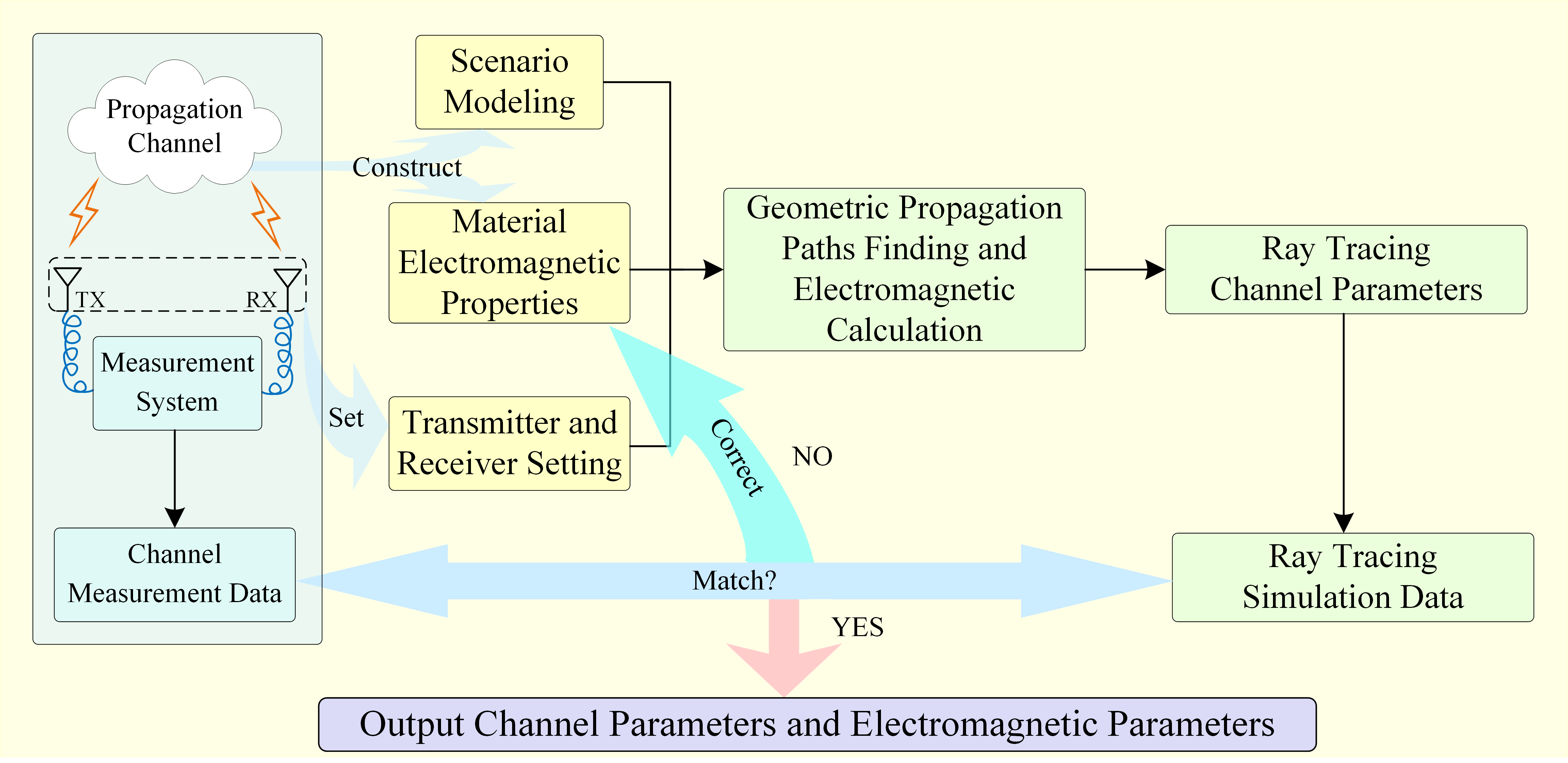
Figure 10: Flowchart of data and model dual-driven channel simulation.

The performance of the data and model dual-driven channel modeling method is demonstrated through a comparison between simulations and channel measurements. Fig. 11 shows the measurement power angle profile, in which five dominant paths are marked in numbers. Furthermore, the delay of five dominant paths is plotted to do the comparison. Fig. 11 shows the results of RT simulations for the five dominant paths. By comparing Fig. 11 with Fig. 11, it can be seen that MPCs have a good agreement in both the spatial and the delay domains between the measurement and RT results. For example, the differences between the measurements and RT simulations for the delay of the five paths are within $\pm$2 ns. And the maximum differences of the angle of arrival (AoA), angle of departure (AoD), delay, and power gain of the dominant paths are $-1.8^{\circ}$, $-1.5^{\circ}$, 0.7 ns and -0.7 dB respectively. Therefore, the data and model dual-driven channel modeling method can well describe the propagation characteristics, i.e., the delay and spatial dispersion, with reduced simulation complexity in THz bands [14].

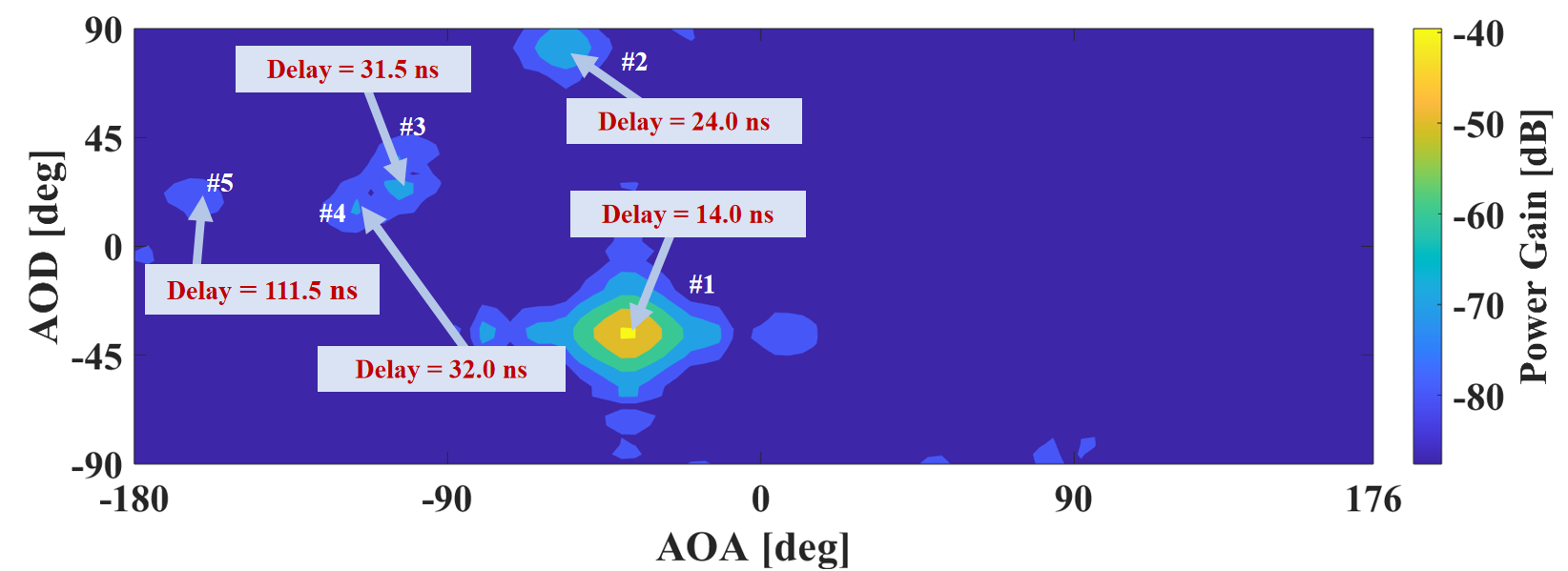
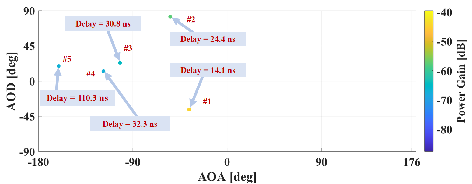
Figure 11: The data and model dual-driven channel modeling method results: a) Power-AoA-AoD measurement result; b) Power-AoD-AoA simulation result.

Hybrid channel models combine deterministic and statistical channel modeling methods, providing a balance between accuracy and efficiency, such as map-based channel model [139], hybrid ray and graph model [140]. For example, due to the sparsity of the THz channel, the main propagation paths of the THz channel (e.g., LoS path and primary reflection path) are generated by the deterministic model, while the other multipaths are generated by the statistical model, which ensures the accuracy of the main propagation paths and quickly obtains the remaining multipath information [141]. Therefore, the hybrid channel model is also not a bad method in THz channel modeling.

III-D Summary and Prospect

In summary, extensive THz channel measurement campaigns have been carried out in typical scenarios such as indoor hotspots, data centers, and outdoor streets from 100 to 450 GHz, and the propagation mechanism characteristics such as THz reflection and scattering as well as channel characteristics have been studied. And we focus on the analysis of THz channel path loss as well as sparsity, which is remarkably different from the sub-6 GHz and mmWave bands. In addition, three methods applied to THz channel modeling are given, namely, statistical, deterministic, and hybrid channel modeling methods, of which the RT-based data and model dual-driven channel modeling method is a promising method. Despite the increasing research on THz channels in recent years, there are still many open issues that motivate future research efforts along the following directions [122].

• High-performance channel sounder: Current THz channel sounders are unable to achieve a balance between measurement accuracy, measurement speed, and measurement distance, which constrains the study of THz channel characteristics. In addition, The existing THz channel measurements are widely used to obtain the omnidirectional channel based on the horn antenna rotation, which is slow and the parameters obtained are not accurate. Therefore, it is necessary to build a THz ultra-massive MIMO array and phased array to achieve accurate parameter estimation as well as fast beam sweeping.

• Analysis and modeling of THz channel characteristics: Increasingly more frequency bands will be deployed and coexist in the future, ranging from sub-6 GHz to 10 THz. In multiband parallel communication systems, it is possible to use the channel characteristics extracted from one frequency band to assist the link establishment of the other band. However, the frequency separation between bands under consideration is large and many channel characteristics variations must be considered. Moreover, the sparsity, near-field characteristics, and non-stationary characteristics in the spatial and frequency domains of the channel due to the short wavelength and high loss are outstanding issues to be modeled, characterized, and incorporated into the channel model.

• Frequency-dependent channel model: The THz bands have a spectrum range of nearly 10 THz, while the 5G channel model supports a frequency range of only 99.5 GHz. Therefore, the channel model of THz bands should be frequency-dependent not only on large-scale parameters but also on small-scale parameters to cover such wide frequency bands. Similarly, the frequency dependence of the characteristics of the THz wave propagation mechanism also deserves in-depth research.

IV Massive MIMO Channel Measurement and Modeling

The complete multi-cellular analysis is given in the limit of an infinite number of antennas, and the concept of massive MIMO is proposed in [142]. Based on the massive MIMO, [143] found that the number of antennas tends to infinity and the favorable propagation is valid under the condition of actual angle distribution. In the 5G era, the three-dimensional (3D) MIMO is considered a promising practical technology, as shown in Fig. 3. The 3D channel model is an extension to the 2D channel model by including elevation angles at both departure and arrival, which makes full use of the elevation domain and increases capacity [144]. It is easier to satisfy favorable propagation conditions with the strong angular spread in azimuth and elevation. In addition, the introduction of vertical dimension has theoretically analyzed the spatial correlation of 3D channel, which is inversely proportional to the vertical space and angular spread value between antenna units, and the capacity of the 3D channel is significantly higher than that of 2D [145], as shown in Fig. 12. In [146], to gain further insight into 3D massive MIMO channels and performance, the field measurements are made on 32 to 256 antenna units at the transmitter and 16 antenna units at the receiver. Based on the channel information extracted from the measurement data, the power angle spectrum, root mean square angle spread, and channel capacity are studied. With the number of antennas increasing, the spatial angle distribution becomes more diffuse, and the channel capacity increases in Fig. 13. Compared with the ideal i.i.d. channel, the capacity of a real massive MIMO channel has a certain capacity difference, and favorable propagation conditions cannot be fully met.

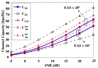
Figure 12: Channel capacity: 3D channel model and 2D channel model.

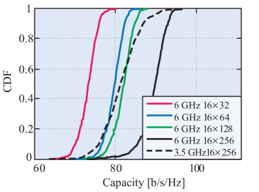
Figure 13: SU-MIMO capacity CDF of 32, 64, 128, and 256 Tx in UMa NLoS.

It can be observed that the massive MIMO technology can significantly increase the wireless transmission data rate, improve the communication quality, and further explore the wireless resources in the space domain. Massive MIMO has more than a hundred antennas at the base station side, forming a large-scale multi-antenna array. It makes full use of spatial freedom, which can effectively improve the transmission capacity and power efficiency of wireless communication systems. With rapid technological innovation and huge business demand, massive MIMO will be further expanded, and the number of antennas will even exceed thousands, forming an ultra-massive MIMO array to bring the change of channel characteristics and models [147, 148]. Therefore, it can be believed that this will widely and deeply reshape the future 6G communication field.

IV-A Massive MIMO Channel Measurement

Currently, the massive MIMO channel measurements fall into two categories. One is to use the virtual antenna array (VAA), the other is to use the real antenna array (RAA). Table II summarizes some massive MIMO channel measurement activities and parameters. Because the real massive MIMO array is not only expensive but also difficult to test antenna patterns due to the large size, the virtual antenna is more common in measurement activities. One is the virtual translation of a single antenna to form a VAA. The antenna array is virtual and consists of a single customized antenna with the help of a mechanical three-dimensional turntable. This method has been adopted in many literatures due to the convenience and easy operation [149, 150, 151]. The other is to use a small antenna array for virtual translation, which can obtain more array elements and is conducive to the analysis of angle domain [146], as shown in Fig. 14. In the measurement with a virtual antenna, there are some problems including the synchronization of the transceiver and receiver and the phase deviation caused by array movement. Compared with the VAA channel, the measurement quantity is relatively smaller, and it can simplify a large number of data processing processes. Besides, the RAA can be used in the channel measurement [152]. This method requires an expensive investment and also needs to consider the problem of massive MIMO antenna calibration.

In addition to the antenna configuration, there are two channel measurement systems, including a frequency domain measurement system based on a vector network analyzer (VNA), and a time domain measurement system based on sliding correlation. The measurement system based on VNA has the advantages of high time domain resolution, internal synchronization of transmitter and receiver, and low complexity. However, this method must connect the transceiver with the VNA, which limits its application in remote outdoor scenarios. In order to solve such problems, some researchers have proposed lengthening the measurement distance of VNA by taking advantage of the low loss characteristics of optical fiber and achieved good results [153]. This system is usually used for massive MIMO channel measurement in indoor hot scenarios, including conference halls, auditoriums, etc. For the time domain measurement system, the channel measurement system based on the sliding correlation method has the advantages of instantaneous broadband measurement, fast measurement, and direct acquisition of time domain results. Although the wired connection between receiver and transmitter is not required in this method, the time and frequency synchronization is required between receiver and transmitter, which makes the system more complex and more difficult to set up [144, 154]. The system is suitable for outdoor long-distance massive MIMO channel measurement activities.

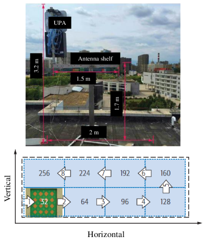
Figure 14: Virtual massive MIMO channel measurement with an antenna array.

TABLE II: Massive MIMO measurements and antenna configurations

Number of array elements	Frequency	Antenna	Channel characteristics	Reference
Tx: 256; Rx: 16	3.5 GHz	VAA	Delay spread	[154]
Tx: 128; Rx: 1	2.6 GHz	VAA, RAA	Capacity, sum-rate, etc	[148, 155]
Tx: 1; Rx: 128	5.6 GHz	VAA	Condition number	[149]
Tx: 128 or 64; Rx: 1 or 4	26 GHz	VAA	Shadow fading, PDP, RMS delay spread, spatial non-stationary	[150]
Tx: 1; Rx: 1600	15 GHz	VAA	K-factor, delay spread, angular spread, spatial non-stationary	[151]
Tx: 256; Rx: 16	3.5, 6 GHz	VAA	Angular spread, capacity, eigenvalue spread	[146, 156]
Tx: 64; Rx: 2	5.8 GHz	RAA	Condition number, spatial non-stationary	[152]
Tx: 720; Rx: 1	26.5-32.5 GHz	VAA	Near-field, spatial non-stationary	[157]
Tx: 8; Rx: 1024	5.3 GHz	RAA	Delay power spectral density, degrees of freedom, etc	[158]
Tx: 1; Rx: 256	11 GHz	VAA	Non-stationarity, spherical wavefront, etc	[159]
Tx: 21$\times$21; Rx: 3$\times$3	26-30 GHz	VAA	Power delay profile, delay spread angular spread, etc	[160]
Tx: 4; Rx: 128	5.3 GHz	RAA	UE correlation, singular value, eigen zero-force power loss, etc	[161]
Tx: 112; Rx: 2	2.6 GHz	VAA	Capacity, achievable rates, correlation coefficient, etc	[162]

IV-B Massive MIMO Channel Characteristics

IV-B1 Near-Field Effect

Since the number of antennas is not very large in the 5G massive MIMO system, the Rayleigh distance of a few meters is negligible. Therefore, the existing 5G communication is mainly developed from far-field communication theory and technology. However, with the significant increase in the number of antennas and carrier frequencies in future 6G systems, the near-field region of massive MIMO will be expanded by orders of magnitude. For example, the 7.3-meter-long virtual linear array is adopted in [163], and the corresponding Rayleigh distance is over 900 m at 2.6 GHz, which is much larger than the radius of a typical 5G cell. Therefore, near-field MIMO communication will become the basic component of the future 6G mobile network, in which the near-field spherical propagation model needs to be considered, which is obviously different from the existing far-field 5G system.

For the near-field effect, the Rayleigh distance of the antenna array needs to be concerned. In general, the Rayleigh distance of an antenna array is defined by $2D^{2}/\lambda$, where $D$ and $\lambda$ are the sizes of the array and carrier wavelength, respectively [164], also known as Fraunhofer distance. In [165], the size of antenna Fresnel and Fraunhofer field regions were systematically derived starting from a general phase factor representation of the scalar diffraction theory. However, with the introduction of new technologies, the near-field range in RIS systems is determined by the harmonic mean of the BS-RIS distance and the RIS-UE distance [166]. Besides, as the antenna array size becomes larger with a large number of antenna elements, the distance between the receiver and transmitter may be shorter than the Rayleigh distance, and the far-field and plane-wave front assumptions in the traditional channel model no longer apply to ultra-massive MIMO. The spherical wavefronts should be considered [167]. The plane wave can be regarded as a long-distance approximation of a spherical wave. In the far-field region, the phase of the electromagnetic wave can be approximated by a linear function of the antenna index by Taylor expansion. In [166], with the plane wavefronts, the far-field beamforming can redirect beam energy to specific angles at different distances. In the near-field region, the phase of the spherical wave is precisely derived based on physical geometry and is a non-linear function of the antenna index. The information on incident angle and distance in each path between BS and UE is embedded in this non-linear phase. In addition, in the near field, massive MIMO can present non-stationary characteristics on arrays [157, 168], which are described in the following section.

IV-B2 Spatial Non-Stationary

Since massive MIMO systems are equipped with large aperture antenna arrays, different channel multipath characteristics can be observed for antenna arrays at different spatial locations, which is called spatial non-stationarity (SnS). In [148], it can be seen that both linear and cylindrical arrays experience large-scale fading over the array. As shown in Fig. 15, the SnS characteristic is observed in massive MIMO channels since the objects in the scenario may no longer serve as complete scatterers for the entire antenna array with its aperture increasing. The SnS characteristics of multipath have been observed in many massive MIMO channel measurements in the literature [157]. As shown in Fig. 15, the different channels are viewed from the elements marked in green and the reference element. Therefore, unlike previous MIMO systems, SnS features are a new challenge introduced in massive MIMO scenarios and must be taken into account in channel modeling [168]. The different antennas at BS can observe different clusters at different times, which can be modeled as a birth-death process [169]. However, for the existing statistical channel models, channel non-stationarity is not considered, or the characterization and interpretation of SnS are not sufficient. Therefore, the channel non-stationary should be dealt with in the channel model of massive MIMO. The SnS research will become more prominent in future ultra-massive MIMO systems for 6G[170].

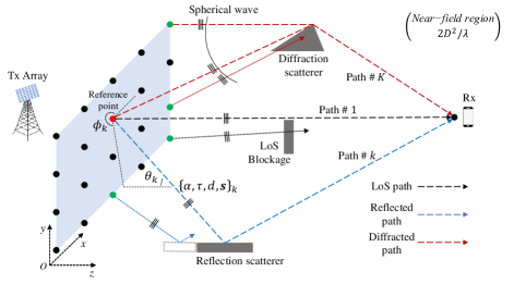
Figure 15: Spherical propagation with the SnS characteristic. Three cases that contribute to the SnS propagation, i.e., LoS blockage, incomplete reflection, and diffraction, are illustrated.

Figure 16: Spatial non-stationary measurement and simulation. (a) RX view in the empty room scenario; (b) Ray trajectories; (c) Power-delay-element measurement result; (d) Power-delay-element simulation result.

IV-C Massive MIMO Channel Modeling

The assumption of plane wave and channel space stationary is used in the 3GPP 38.901 channel model of 5G, which is mainly aimed at small-scale MIMO systems [171]. However, these assumptions will be challenged in massive MIMO systems, even ultra-massive MIMO systems. The expanded array size would result in a violation of the Fraunhofer distance in a real deployment scenario. In this case, the UE or scatterer is most likely to be in the near field of the base station, so the more general spherical wave model should be considered for the channel modeling.

Statistical channel modeling is an important modeling method for massive MIMO channel modeling, which can be further divided into correlation-based stochastic model (CBSM) and geometry-based stochastic model (GBSM). Due to the low complexity and limited precision, the CBSM is not enough to simulate the above non-stationary phenomena or spherical wave effect. The GBSM is more practical because of its relatively higher accuracy. In [172], second-order approximate channel models of spherical wavefronts (i.e. parabolic wavefronts) for massive MIMO channels are established in both spatial and temporal domains to effectively simulate near-field effects. In [158], the general three-dimensional (3D) non-stationary GBSM for ultra-massive MIMO communication systems is proposed in 6G communication. Based on the complex principal component analysis (PCA) method in machine learning, the principle is to maximize the converted channel power, extract representative channel features, and use these features to ultimately reconstruct CIR [173]. The proposed method is robust with the increase of antennas, which provides insights for future massive MIMO channel modeling. In addition, the COST 2100 model is a cluster-level GBSM for the MIMO system, which is the first to use the concept of visible region (VR) [174] to simulate spatial non-stationarity along the antenna array. The cluster can only be viewed through the antenna element located in the corresponding VR. However, due to the plane wave hypothesis, the modeling precision of spatial non-stationary characteristics is limited in COST 2100 model. Based on the concept of VR, the GBSM with different frequency bands and scenarios is used to represent spatial non-stationary and near-field effects for the large-scale array configuration [159]. However, the validity of these models needs to be further verified by measurements in real scenarios.

In order to reduce the complexity of massive MIMO channel modeling, [157] proposes the massive MIMO channel modeling framework based on the capture and observation of multipath propagation mechanisms (i.e., LOS, reflection, and diffraction). As shown in Fig. 16, it can be observed that the spherical propagation with the SnS characteristic is based on the measurement and ray-tracing simulation. Fig. 16 shows the measurement and simulation environment. Fig. 16(b) shows the ray trajectories diagrams of the dominant path. The trajectory color changes in the order of red-orange-yellow-green indicating that the received power decreases sequentially. Compared with the traditional static channel modeling, only one additional SnS parameter is added to the proposed framework, which is required for low-complexity implementation. This method has good real-time performance, low complexity, and accuracy. In [157], there exist $K$ SnS spherical propagation paths between the Tx array and the Rx. The massive MIMO channel at the frequency $f$ can be modeled as a superposition of CFRs of the $K$ paths on the array, which can be expressed as

$$\begin{split}H^{sns}(f)&=S\odot A(f)\cdot H(f)\end{split}$$ (19)

where $H^{sns}(f)$ comprises $M$ complex values, i.e., $H^{sns}(f)\in C^{M\times 1}$, $f\in[f_{L},f_{U}]$ is the frequency within the designed range, and $\odot$ represents elementwise product operation. $H(f)\in C^{K\times 1}$ denote CFRs at $f$ of the $K$ paths at the reference point (in Fig. 15)

$$\begin{split}H(f)&=[\alpha_{1}e^{-j2\pi f\tau_{1}},...,\alpha_{k}e^{-j2\pi f\tau_{k}},...,\alpha_{K}e^{-j2\pi f\tau_{K}}]^{T}\end{split}$$ (20)

where $\alpha_{k}$ and $\tau_{k}$ represent the complex amplitude and propagation delay of the $k$th path, respectively. $(\cdot)^{T}$ denotes the transpose operation. A novel matrix $S$ is introduced in the proposed modeling framework for the SnS property. It contains $K$ nonnegative real-valued vectors, i.e.,

$$\begin{split}S&=[S_{1},...,S_{k},...,S_{K}]\end{split}$$ (21)

where $s_{k}=[s_{1,k},...,s_{m,k},...,s_{M,k}]^{T}$ and $s_{m,k}$ is the SnS property of the $k$th path on the $m$th element. In Fig. 16(c) and (d), the power and delay of MPCs vary with the element, exhibiting a non-stationary characteristic in the spatial domain. Besides, the delay differences between the three dominant paths are 0.1 ns and the power differences are within 0.3 dB, which verifies the accuracy of the channel modeling method.

Compared with statistical channel modeling, deterministic channel modeling can accurately capture electromagnetic wave propagation characteristics. No matter the size of massive MIMO antenna arrays, the RT method can accurately capture channel characteristics, which makes it a promising channel modeling method for massive MIMO systems [175, 176]. However, only a few works have implemented RT to characterize channels with large array configurations. The reason is that the arrays on the Tx and Rx side are usually obtained by strong simulation of each Tx and Rx antenna pair in RT. The computational complexity is particularly challenging for massive MIMO systems because it increases linearly with the number of array elements. At present, the map-based model is proposed to implement the RT method, which can effectively reduce the computational complexity by simplifying the geometry and electromagnetic description of the environment and restricting the sequence of interactions between the rays and objects [177]. The model may have poor accuracy in predicting the channel at specific locations, but it is fully capable of simulating the non-stationarity and transition of large arrays. However, the strategy is hard to capture the spatial non-stationarity between array elements (i.e. ray birth-death process).

In addition, the hybrid modeling method combining statistical and deterministic modeling is also expected to reduce the complexity of the model because only the dominant path has RT characteristics, but the key issue is the simplicity and accuracy of channel modeling.

IV-D Summary and Prospect

The massive MIMO channel measurement mainly adopts a frequency domain or time domain channel measurement system based on the virtual antenna. With the increase of the 6G spectrum, Rayleigh distance increases, and near-field effects and spatial non-stationary characteristics are more likely to appear. To address these characteristics of massive MIMO, statistical modeling and deterministic modeling have been carried out and some achievements have been made, but there are still many unsolved problems and challenges. This section summarizes the research method, new characteristics, and modeling method, and points out several future research directions for massive MIMO.

• Channel research method: The channel measurement method based on RAA is faced with the challenge that the cost and complexity will become extremely high with the increase of antenna array. There are many dynamic application scenarios in 6G, but the current VAA measurement method is difficult to meet the measurement requirements of a massive MIMO system in a dynamic environment. In addition, the phase sensitivity of large array antennas should be considered. Therefore, exploring a dynamic channel detection system is worthy of further study.

• Channel characteristics: The spatial non-stationary characteristics are the basic feature of massive MIMO. How to better describe spatial non-stationary characteristics on arrays is also an important work in 6G channel research. In addition, the impact of new technologies in near-field communication (such as RIS assisted near field communication) has not been fully studied. For some performance metrics, such as capacity, the classical Rayleigh distance may not capture the performance loss of these metrics well.

• Channel modeling: In real systems, both far-field and near-field signals are usually present in the communication environment. Compared with plane wave modeling, the spherical wave model can be introduced to solve the near-field effect, but the model is too complicated. The deterministic modeling method can accurately capture massive MIMO channel features, but the computational complexity may be relatively higher. To balance the relationship between complexity and accuracy, or to flexibly choose modeling methods according to the needs of the system, the corresponding solutions should be given in future work.

V JCAS channel measurement and modeling

Figure 17: The illustration of JCAS channel model and new characteristics. The dashed lines indicate that the paths are interrupted.

Fig. 17 shows the illustration of the JCAS channel and highlights new characteristics introduced by JCAS systems and applications. This channel considers a typical JCAS scenario with one base station (BS) and one mobile terminal. The BS can achieve the transmission and reception of sensing signals, as well as the transmission of communication signals. The terminal only has the function of receiving communication and sensing signals. In the subsequent description, we use TX and RX to describe the communication link. BS-TX and BS-RX describe sensing link. The blue lines denote communication paths in this model, and the red lines denote sensing paths. The dashed lines indicate that the paths are interrupted. The sensing channel includes propagation paths from BS-TX to scatterers and back from scatterers to BS-RX. When the sensing signal is received by the BS-RX, this sensing mode is called active sensing, and when the sensing signal is received by RX (no sharing data with the BS-TX), it is called passive sensing. New characteristics or changes such as RCS, Doppler, environment effect, and the shared cluster are also represented in the scenario. Subsequent characteristics descriptions, as well as modeling, are based on Fig. 17.

V-A JCAS Channel Measurements

Channel measurement is an effective way to understand and extract the JCAS channel characteristics. At present, many researchers have measured JCAS channels focusing on various perspectives such as frequency, scenario, and sensing mode. As the sensing modes lead to the different measurement methods, measurement activities of JCAS channels are summarized in terms of active and passive sensing.

To simulate active sensing, researchers place the transmitter (TX) and receiver (RX) in the same position for channel measurement. Physical isolation is used to eliminate the mutual influence of the TX and RX antennas. The team at the Tampere University in Finland uses this approach to operate TX and RX as a JCAS system, scanning its surrounding environment while steering its beam pattern towards different directions and observing the target reflections[178]. L. Pucci measures the sensing channel in this way and finds that the received signal strength is affected by the sensing target, and the self-transmitting and self-receiving sensing channel will produce self-interference, which should be portrayed in the JCAS channel model [179]. Moreover, Some scholars also conduct measurements to investigate and model the path loss in the sensing channel under the active sensing mode [180]. The Range-Power profile, Range-Doppler spectrum, and Range-Angle spectrum are obtained and analyzed in the sensing measurement[181, 182].

Another mode of sensing is passive sensing, where BS-TX and BS-RX are placed in different positions to sense the environment or target. In [183], the cluster power attenuation factors, which is a new parameter of the JCAS channels, is measured under the passive sensing mode. Small-scale fading is one of the important characteristics of the channel, which has been measured and modeled by J. Salmi [184], this will provide help for the unity modeling of the JCAS channel. As for the Doppler characteristics of the channel, N. Avazov studies it under the passive sensing mode and models it based on the measured data [185]. Sun et al. use this method to reconstruct the indoor environment, utilizing the AoDs and AoAs information of the sensing channel [186]. Based on the above measurement activities, researchers have begun to make preliminary research on sensing channel characteristics under active or passive sensing mode. However, the current measurement activities mostly focus on recognizing traditional features while lacking the introduction of new features in JCAS channels.

The detailed summary of measurement activities is shown in Table III, which outlines the scenarios, sensing modes, and channel characteristics of JCAS measurement activities. From the table, this article lists some conclusions in the following. Firstly, JCAS channel measurement research in the mm-wave band is still mainstream. However, THz is considered a potential sensing frequency band due to its large bandwidth, which has attracted the wide attention of scholars [187]. Secondly, for the measurement methods, the frequency domain VNA-based sounder and the correlation-based time-domain channel sounders are two primary methods to measure the JCAS channel [183]. Thirdly, measurement scenarios are mainly divided into indoor and outdoor measurements, but detailed scenarios are related to the application of JCAS [188]. Finally, the current measurement activities of active sensing are more practical than those of passive sensing. Due to the differences in the propagation configuration of the sensing and communication channels, the delay, path loss, and Doppler characteristics of the sensing channel may differ from those of the communication channel. At the same time, some new characteristics, such as RCS and self-interference, should also be considered in the sensing channel.

TABLE III: JSAC channel measurement campaigns

Frequency	Bandwidth	Domain	Scenario	Sensing mode	Characteristics	Ref.
0.1-3 GHz	2.9 GHz	Time	Outdoor	Active	Path loss, delay, AoA.	[180]
28 GHz	1 GHz	Time	Indoor	Active	Delay, Doppler, RCS, AoA, AoD.	[178]
3.5/28 GHz	Not mentioned	Time	Outdoor	Active	AoA, AoD, Doppler, RCS.	[179]
73 GHz	2 GHz	Time	Indoor	Active	Path loss, delay, AoA, AoD, power.	[181]
57.5-63.5 GHz	6 GHz	Frequency	Indoor	Active	Delay, AoA, ToA.	[182]
2-8 GHz	300 Hz	Frequency	Indoor	Passive	Power, azimuth angle, antenna positions.	[184]
77 GHz	2 GHz	Time	Outdoor	Passive	Power, delay, Doppler, RCS.	[183]
24 GHz	250 MHz	Time	Indoor	Passive	Doppler, path loss.	[185]
60 GHz	100 MHz	Time	Indoor	Passive	AoA, AoD, path loss.	[186]

V-B JCAS Channel Characteristic Research

V-B1 Sensing target characteristics

Due to the purpose of sensing is to obtain information about the target, target characteristics parameters are part of the sensing channel and need to be analytically modeled. In the existing research, modeling the target characteristics as RCS parameter is the mainstream way to describe the target in the sensing channel. RCS represents the interception and scattering ability of the target to the signal power. For the JCAS system, RCS will have a great impact on the received power of the signal, and also affect the cluster characteristics of the sensing channel and communication channel. Therefore, methods based on measurements or deterministic modeling are used to model RCS. Researchers in [189] propose a modeling method for sensing targets, and the method is verified by actual measurement. Most of the current studies on RCS are based on far-field assumptions. Many papers have studied by assuming that the electromagnetic wave reaching the target is a plane wave. However, in JCAS applications, the distance between the target and the sensing TX / RX is relatively close, resulting in most of the targets being located in the near field of the antenna. A comprehensive RCS unity model must be developed, encompassing both near and far field properties, to effectively apply to diverse targets within the JCAS systems.

V-B2 Doppler effects

To achieve high-precision sensing, the JCAS system requires support from high carrier frequencies. However, the Doppler spread effect, which is proportional to the carrier frequency, becomes even more stringent in the JCAS systems, particularly in high-mobility scenarios. Some current literature has taken into account the differences in Doppler parameter of JCAS channels [186]. If JCAS technology is implemented in a widely used OFDM system, the sensing channel with high Doppler propagation may disrupt subcarrier orthogonality and cause intercarrier interference, while the accuracy of the speed estimate is reduced. In summary, accurately modeling of Doppler characteristics in the JCAS channel model poses a significant challenge.

V-B3 The environmental effect

Figure 18: Target response measurement campaign and results. (a) Measurement scenario layout. (b) The power delay profile of measurement result.

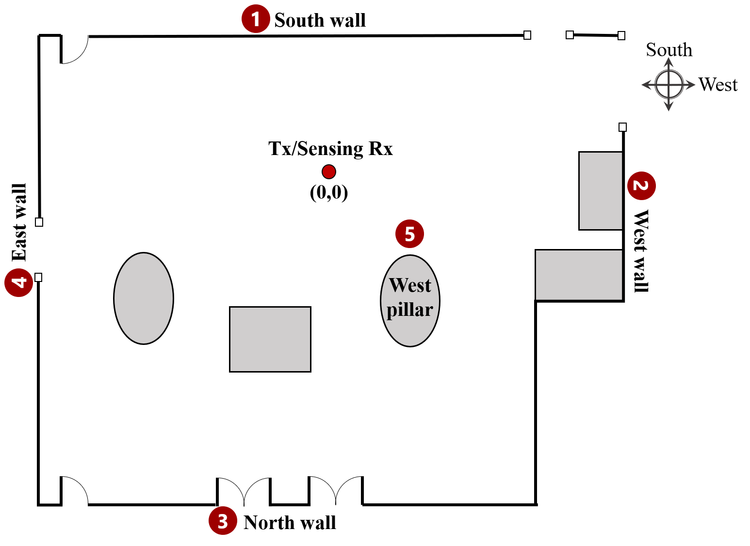
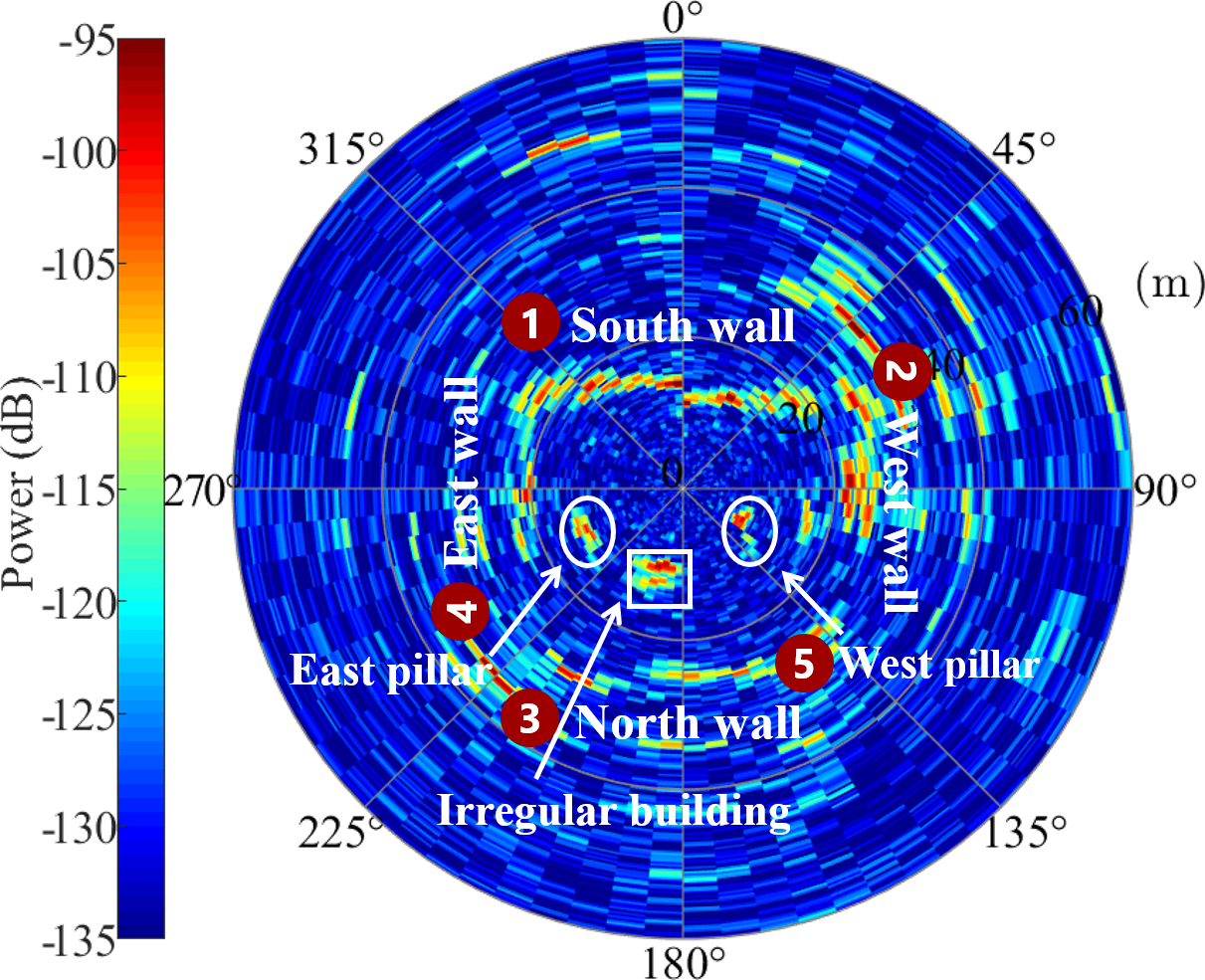
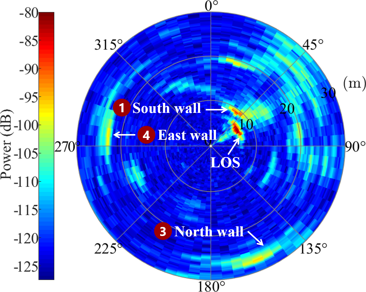
Figure 19: Shared scatterers measurement campaign and results. (a) Sensing and communication measurement environment in the indoor hall. (b) Sensing PADP. (c) Communication PADP.

The channel is highly affected by the surrounding environment, and it is crucial to pay attention to this effect. In the JCAS systems, sensing aims at obtaining information about the target in the environment, and during this process, the environment information is coupled with the channel data, affecting the target information extraction. The authors in [190] explore the impact of the environment by performing metal-interfered and non-interfered measurements in an outdoor road, and the measurement scenario layout is shown in Fig. 18(a). The red dots in Fig. 18(a) represent the measurement positions of Scheme 1 to research the effect of the environment on the sensing channel at different distances. The channel impulse responses (CIRs) of each distance are stitched to obtain the measured power-delay profile. The power of the LoS path in Fig. 18(b), which is shaped by the sensed target, decreases significantly with increasing distance and determines whether the channel can sense the target from the environment. The purple dots and stars represent the stationary sensed target and the moving metal interference of Scheme 2, respectively, to investigate the effect of the interference on the sensing channel at different distances. When the interference is close to the target, the sensing channel will change greatly. The numerical labels in the fig. 18(b) represent other multipath in the environment. To quantify the variant of the environment around the sensed target and the proportion of LoS path in the multipath, the power ratio (PR), which is the ratio of the sensed target power and the sum of the effective environmental power is defined. Results show that whether the target can be sensed depends on the ratio of the target power in the sum of environment multipath powers. However, incorporating the influence of the environment into the JCAS channel model remains a challenge.

$$h_{c}(\theta_{c,R},\theta_{c,T},\tau_{c})= \underbrace{\sum\limits_{n_{0}=1}^{N_{0}}\sum\limits_{m_{0}=1}^{M_{0}}a_{c,n_{0},m_{0}}\delta(\theta_{c,R}-\theta_{c,n_{0},m_{0},R})\delta(\theta_{c,T}-\theta_{c,n_{0},m_{0},T})\delta(\tau_{c}-\tau_{c,n_{0},m_{0}})}_{\text{Shared\ Communication\ Sub-Clusters}}$$

$$+\sum\limits_{n_{1}=1}^{N_{1}}\sum\limits_{m_{1}=1}^{M_{1}}a_{c,n_{1},m_{1}}\delta(\theta_{c,R}-\theta_{c,n_{1},m_{1},R})\delta(\theta_{c,T}-\theta_{c,n_{1},m_{1},T})\delta(\tau_{c}-\tau_{c,n_{1},m_{1}}),$$ (22a)

$$h_{s}(\theta_{s,R},\theta_{s,T},\tau_{s})= \underbrace{\sum\limits_{n_{0}=1}^{N_{0}}\sum\limits_{m_{0}=1}^{M_{0}}a_{s,n_{0},m_{0}}\sigma_{n_{0},m_{0}}\delta(\theta_{s,R}-\theta_{s,n_{0},m_{0},R})\delta(\theta_{s,T}-\theta_{s,n_{0},m_{0},T})\delta(\tau_{s}-\tau_{s,n_{0},m_{0}})}_{\text{Shared\ Sensing\ Sub-Clusters}}$$

$$+\sum\limits_{n_{2}=1}^{N_{2}}\sum\limits_{m_{2}=1}^{M_{2}}a_{s,n_{2},m_{2}}\sigma_{n_{2},m_{2}}\delta(\theta_{s,R}-\theta_{s,n_{2},m_{2},R})\delta(\theta_{s,T}-\theta_{s,n_{2},m_{2},T})\delta(\tau_{s}-\tau_{s,n_{2},m_{2}}).$$ (22b)

V-B4 Shared cluster characteristics

There are many scatterers in the environment, some of which will affect communication, and some of which are the target of sensing in JCAS systems. Therefore, the overlapping scatterers acting for both communication and sensing channels can be defined as the shared scatterers, as shown in Fig. 17. These shared scatterers have been validated and analyzed through realistic JCAS channel measurement campaigns conducted in [191]. Fig. 19(a) illustrates the layout of the JCAS channel measurement scenario, with primary scatterers identified by red sequence numbers. Based on the CIRs obtained through measurements, the power-angular-delay profiles (PADPs) are calculated, as shown in Fig. 19(b) (c). As can be seen from Fig. 19, the sensing clusters corresponding to the scatterers reflect the realistic environment, while the communication clusters indicate the scatterers contributing to the communication channel. Some scatterers are shared between the sensing channel and communication channel, i.e. the south wall, the north wall, and the east wall. Therefore, the shared clusters generated by these shared scatterers reveal the realistic sharing feature of communication and sensing channels, which need to be adequately considered in channel modeling for JCAS systems.

V-C JCAS Channel Modeling

To model the channel for the JCAS systems, the channel modeling method of the 5G system mentioned above needs to be extended. Firstly, the JCAS channel model needs to include RCS, which can be introduced into the large-scale part of the model from the perspective of the RCS mechanism. Secondly, the Doppler parameter needs to be extended based on the communication model. Thirdly, for the influence of the environment, it is necessary to introduce relevant parameters, such as PR, into the JCAS channel model to characterize after small-scale modeling. As for the shared cluster characteristics of the JCAS channel, a shared cluster-based stochastic channel model is proposed in [191]. This model is expressed by the superposition of shared and non-shared clusters to capture the sharing feature, and also includes RCS features. The sharing degree (SD) metric is introduced to define the power ratio of the shared clusters in the channels.

As illustrated in Fig. 17, the clusters which experience the shared scatterers in both the communication and sensing channels are defined as the shared clusters of JCAS channels. The specific formula expressions are given by Equ. 22. and Equ. 22. In this model, $h_{c}(\theta_{c,R},\theta_{c,T},\tau_{c})$ and $h_{s}(\theta_{s,R},\theta_{s,T},\tau_{s})$ denote the CIR of communication and sensing. The subscripts, $c$ and $s$, denote the communication and sensing propagations, respectively. $\delta(\cdot)$ denotes the Dirac Delta function. $a$ and $\tau$ are employed to describe the complex amplitude and time delay of communication and sensing MPCs. $\theta$ denotes azimuth transceiver angle of MPCs, where $\theta_{T}$ represents the AOD, $\theta_{R}$ represents the AOA. A detailed explanation of this formula can be found in [191].

In the proposed JCAS channel model, the sensing channel and communication channels are generated independently, but they are partially coupled with each other, which also provides insights for the subsequent JCAS channel model based on 3GPP standard extension. Moreover, due to the changes in channel topology, parameters such as delay and angle spread in 3GPP standard channel model need to be modified. At the same time, the aforementioned JCAS channel characteristics should also be taken into account in channel modeling, which is not currently addressed in communication channel models.

V-D Summary and Prospect

JCAS channel measurement mainly focuses on frequency or time domain, and the measurement methods are classified into active and passive sensing. With the integration of sensing and communication, RCS, Doppler, environment effects and shared cluster characteristics are important in the JCAS channel. To capture these characteristics of JCAS channels, a preliminary statistical channel model has been carried out [191] and some modeling views have been proposed. However, there are still many aspects that require further research. This subsection summarizes the current progress of the JCAS channel measurement, new characteristics, and modeling, and points out several future research directions for JCAS development.

V-D1 Channel measurement

Channel measurement is an effective method to extract the characteristics of JCAS channels. However, there are few measurement activities for JCAS channels in the existing literature. This is due to a lack of understanding of the JCAS channel and the requirement for an upgraded measurement platform. The existing measurement platform has limitations in the antenna configuration, waveform selection, measurement scheme design, and other aspects of the defects. JCAS channel measurement requires accurate capture of sensing and communication channels in large bandwidth and high-frequency bands, which presents challenges in generating and receiving two channels simultaneously, storing large amounts of data and calibrating the system. Additionally, the shared integration mode is a major challenge for JCAS channel data acquisition.

V-D2 Channel characteristics

The study of JCAS channel characteristics is based on practical measurement results. Existing papers on JCAS channel characteristics mainly focus on traditional communication channel characteristics, such as time delay and angle spread, which are inadequate for a comprehensive understanding of the JCAS channel. Therefore, further research is required to explore new characteristics, including shared scatterers, target modeling, clutter modeling, correlation, and other aspects. Moreover, it is necessary to incorporate these features into the JCAS channel model.

V-D3 Channel modeling

In terms of JCAS channel modeling, the communication channel model has been well developed, therefore the extension based on the communication channel model is a mainstream way. The JCAS channel model is supported by supplementing the modeling process and parameters. However, environment reconstruction-based channel modeling [192], map-based hybrid channel modeling [193], and standard extension-based channel modeling are the potential research directions in JCAS channel modeling. Moreover, the combination of JCAS channel modeling with other emerging technologies, such as RIS and NOMA, is a potential direction for future research.

VI RIS Channel Measurement and Modeling

Compared with traditional wireless communication technologies, RIS provides a new dimension for wireless communication system design, but it also introduces complexity to channels. Fig. 20 shows a typical RIS-assisted communication scenario. In the scenario, the LOS path is occluded and a RIS is used to boost the received signal. Notably, the RIS channel is characterized by a Tx-RIS-Rx cascade channel, which is composed of the Tx-RIS sub-channel, RIS-Rx sub-channel, and RIS response.

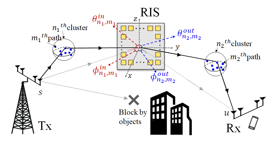
Figure 20: A typical RIS-assisted communication scenario.

VI-A RIS Channel Measurements

The introduction of RIS brings new challenges for channel measurements. The high path loss caused by cascaded channels requires higher transmission power and dynamic range of the measurement platform. In addition, the measurement platform must be more flexible in order to cope with the complex application scenarios of RIS.

Currently, a few researches on RIS channels based on channel measurements have been carried out. These measurements are mostly taken in microwave anechoic chambers and practical scenarios, and most of them focus on the large-scale characteristics of RIS channels. In [194], authors carry out a path loss measurement in a microwave anechoic chamber and utilize three different meta-surfaces to act as RISs in different scenarios. This work measures the free-space path loss in the RIS-assisted broadcasting and beamforming scenarios and compares it with the theoretical model. Some of the other measurement campaigns are carried out in practical scenarios. A near-field RIS channel measurement is carried out in indoor and outdoor environments to research the path loss characteristics of RIS channel [195]. To facilitate channel modeling in system simulations, [196] proposes a reflective RIS physical model and conducts indoor RIS measurement. This work realizes the abstraction of the RIS physical model for application in channel modeling in a practical scenario.

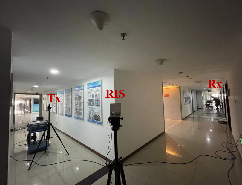
Figure 21: The RIS channel measurement in a corridor scenario.

The authors in [197] build a RIS-assisted channel measurement platform that can be applied to various complex scenarios based on the time domain correlation principle. With this platform, the authors carry out a channel measurement in a typical indoor corridor scenario at 26 GHz, as shown in Fig. 21. They research the path loss characteristic of RIS-assisted channels in corridor scenarios based on the measurement data, as shown in Fig. 22. The results indicate that a modified version of the multiplicative-distance model can effectively fit the measurement data in this RIS channel:

$$PL(d_{tx},d_{rx})=\begin{cases}20.94{\rm{log}_{10}}(d_{tx})+22.34{\rm{log}_{10}}(d_{rx})+63.59,\\ \vspace{1ex}\hfill{\text{ $d_{rx}{\leq}{18.6{\,}\rm{m}}$ },}\\ \vspace{1ex}20.94{\rm{log}_{10}}(d_{tx})+14.83{\rm{log}_{10}}(d_{rx})+73.12,\\ \vspace{1ex}\hfill{\text{ $d_{rx}{\geq}{18.6{\,}\rm{m}}$ },}\end{cases}$$ (23)

where $d_{tx}$ represents the distance from Tx to RIS and $d_{rx}$ represents the distance from RIS to Rx respectively.

Table IV summarizes the measurement campaigns in detail. The current focus of RIS measurement research is on the large-scale characteristics and the primary purpose of measurement campaigns is model verification. In terms of measurement frequency, measurement campaigns are mostly carried out in sub-6 GHz and millimeter band, which is restricted by RIS.

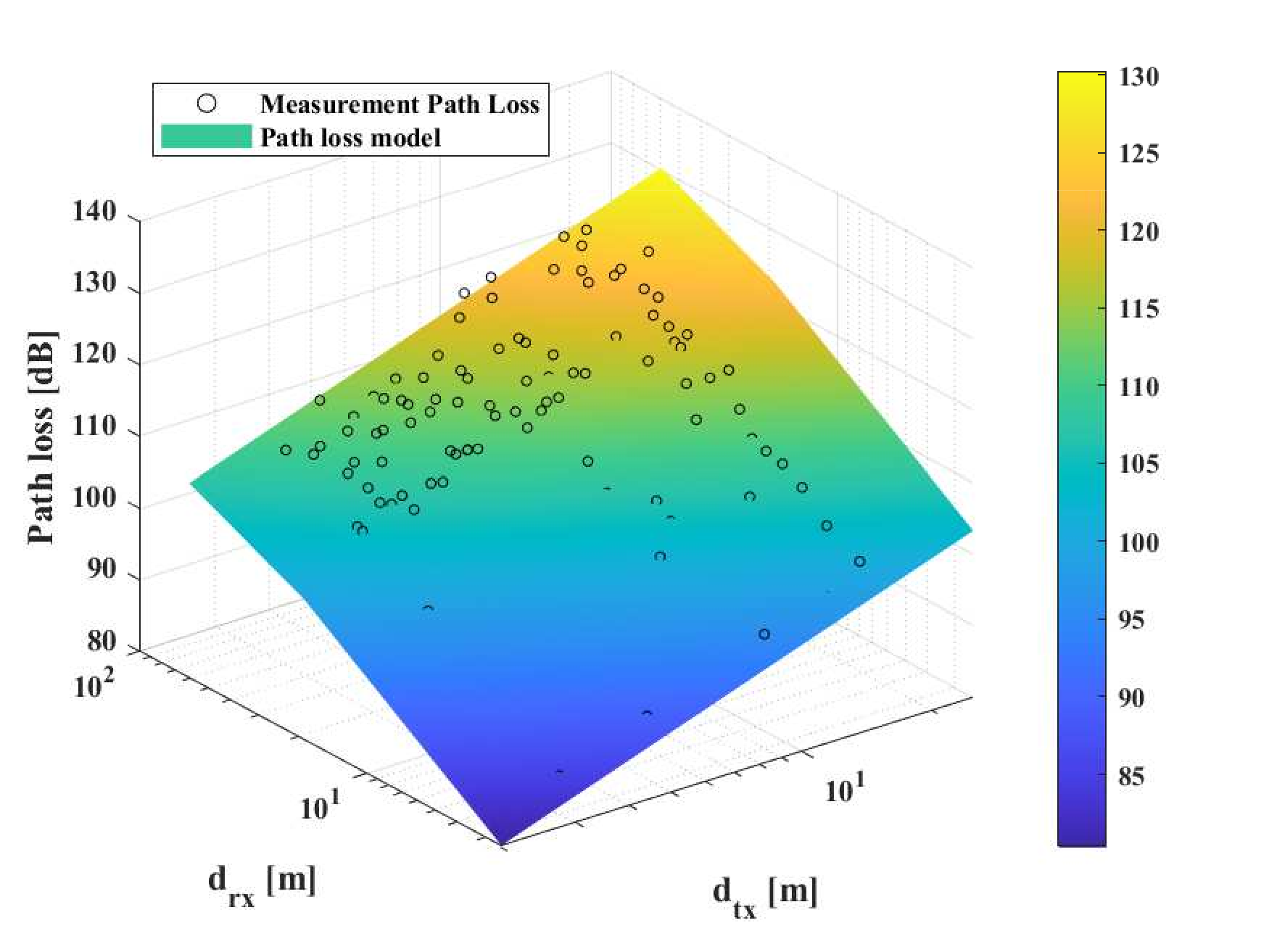
Figure 22: The measurement data and path loss model of RIS-assisted channel in a corridor scenario at 26 GHz.

TABLE IV: RIS measurement campaigns

Frequency	Continuous/Discrete Phase	Scenario	Characteristics	Purpose	Ref.
4.25/10.5 GHz	Continuous	Microwave anechoic chamber	Power	Model verification	[198]
5.8 GHz	Discrete	Indoor, Outdoor	Path loss	Model verification	[195]
26.9 GHz	Discrete	Indoor	Power	Model verification	[196]
27/33 GHz	Continuous	Microwave anechoic chamber	Power	Model verification	[194]
5.8 GHz	Continuous	Microwave anechoic chamber, Indoor, Outdoor	Power, Radiation pattern	Parameter analysis	[199]
26 GHz	Discrete	Indoor	Path loss	Parameter analysis	[197]

VI-B RIS Response and Channel Characteristics

In RIS-assisted communication, two key features require special attention. The first is the RIS response characteristics, which reflect the interaction between the RIS and the signal. The second is the traditional channel characteristics following the introduction of RIS, such as path loss, which may differ from conventional models.

VI-B1 RIS response characteristics

The RIS response comprises two components: the overall response of the RIS, which is represented by the RIS radiation pattern, and the response of the RIS element. As the overall response is a synthesis of each element’s response, investigating the response characteristics of the RIS element is critical. Specifically, the reflection coefficient characteristics and radiation pattern of the RIS element require close attention, as they directly affect the accuracy of the overall response synthesis.

$\bullet$ Reflection coefficient characteristics

The reflection coefficient characteristics of the RIS element are depicted by hardware models. In the initial research of RIS-assisted communication, the hardware model of the RIS element is usually the ideal regulator model. This means that The RIS element exhibits the same reflection coefficient regardless of the angle and polarization of the incident signal. However, by comparing the Fresnel reflection coefficient, it can be found that the incident angle and polarization dependence of the RIS element reflection coefficient may be ignored. Fresnel reflection coefficient is widely used to characterize the reflective properties of 3D materials. Generally speaking, the Fresnel reflection coefficient is related to the polarization and angle of the incident signal, as demonstrated by formulas (9) and (10). In fact, for the 2D RIS element, its reflection coefficients also exhibit such dependence on incident angle and polarization.

To more accurately characterize the RIS element reflection coefficient characteristics, some electromagnetic hardware models have been proposed, including transmission line model[200], equivalent circuit model[201, 202], generalized sheet transmission conditions (GSTCs) model [203], and load impedance model [204].

In the transmission line model, the tangential component of electric and magnetic fields are equivalent to voltage and current, and then the relationship between reflection coefficient and incident angle and polarization direction can be deduced according to Kirchhoff formula[200]. The equivalent circuit model is similar to the transmission line model, where the RIS element is equivalent to a circuit. Since the impedance in the circuit is related to the incident angle, the reflection coefficient is also naturally related to the incident angle [201]. The GSTCs model is widely used in the metasurface field. It uses the surface susceptibilities tensor as the characteristic parameter of the RIS element and then combines the GSTCs condition to calculate the reflection coefficient corresponding to the incident signal of any incident angle and polarization direction[203]. The load impedance model regards the RIS element as a thin surface with a certain electric and magnetic impedance. Its principle is shown in Fig. 23, that is, under the excitation of the incident signal, the induced electric and magnetic currents are generated on the RIS element, and they become new radiation sources that radiate electromagnetic waves outward, making the RIS element exhibit a certain reflection coefficient. Since the induced electric and magnetic currents are jointly determined by the electric impedance, magnetic impedance, incident angle, and polarization direction, the reflection coefficient is affected by the incident angle and polarization direction of the incident signal[204].

In the load impedance model, the reflection coefficient for the vertically polarized signal is written as

$$R_{v}(\theta_{in})=\frac{-\eta}{2Z_{e}cos\theta_{i}+\eta}+\frac{Z_{m}cos\theta_{i}}{Z_{m}cos\theta_{i}+2\eta}.$$ (24)

Correspondingly, if the incident signal is parallel polarized, the reflection coefficient is written as

$$R_{h}(\theta_{in})=\frac{\eta cos\theta_{i}}{2Z_{e}+\eta cos\theta_{i}}-\frac{Z_{m}}{Z_{m}+2\eta cos\theta_{i}},$$ (25)

where $Z_{e}$ and $Z_{m}$ are electrical impedance and magnetic impedance, $\eta$ is the wave impedance in the propagating medium.

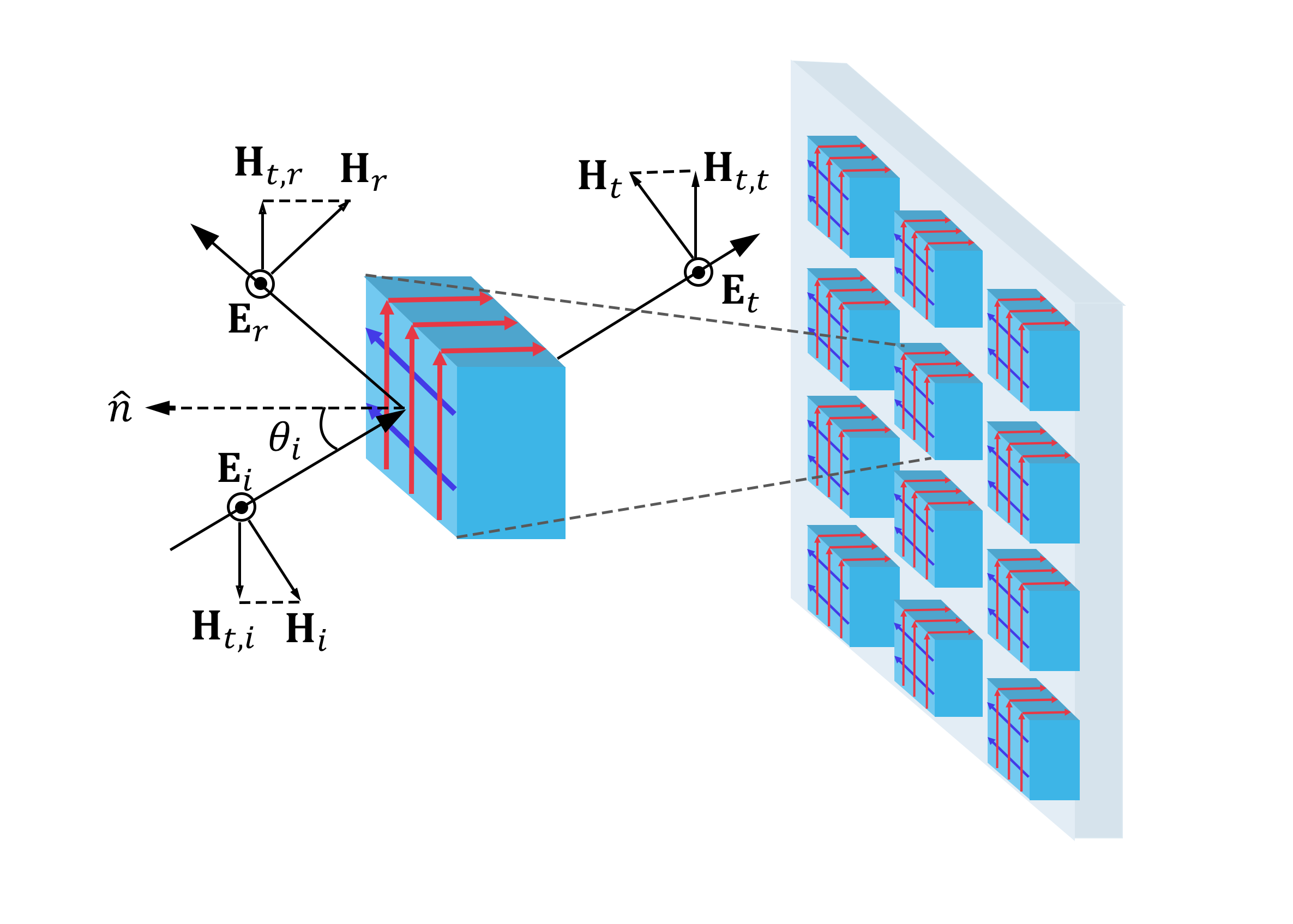
Figure 23: Load impedance model of RIS [204].

$\bullet$ RIS element radiation pattern modeling

RIS technology can direct the beam in the desired direction by adjusting the reflection coefficient of each element. This is achieved by ensuring that the scattered signal of each element has constructive interference in the desired direction and destructive interference in other directions. To accurately describe this process, it is necessary to model the distribution of the scattered field generated by each RIS element in all directions, that is, the RIS element radiation pattern. Currently, there are two commonly used methods for modeling the RIS element radiation pattern, namely, mathematical function fitting and electromagnetic scattering theory calculation. In [205] and [194], the RIS element radiation pattern is fitted by the $cos^{q}\theta$ function. In [204], [206], and [196], the physical optics method (PO) is used to calculate the radiation pattern of the RIS element. In [195],[207], the radiation pattern of the RIS element is modeled by calculating its RCS. In [208], the electromagnetic equivalence principle is employed to calculate the RIS element radiation pattern.

Taking the model presented in [208] as an example, we introduce the radiation pattern modeling process of RIS elements in the following. Assuming that a signal with both vertical and parallel polarization components is incident on a RIS element at a horizontal angle $\phi_{in}$ and a vertical angle $\theta_{in}$, its electric field is $\mathbf{E}_{i}$, and its corresponding magnetic field is $\mathbf{H}_{i}$. Thus, according to equivalence theore, the equivalent current $\mathbf{J}_{s}$ and equivalent magnetic current $\mathbf{M}_{s}$ of the RIS element are calculated as

$$\mathbf{J}_{s}= \hat{\bm{n}}\times(\mathbf{H}_{i}+\mathbf{H}_{r}),$$ (26)

$$\mathbf{M}_{s}= -\hat{\bm{n}}\times(\mathbf{E}_{i}+\mathbf{E}_{r}),$$

where $\mathbf{E}_{r}$ and $\mathbf{H}_{r}$ represent the reflected electric and magnetic fields, which are obtained from the reflection coefficient of the RIS element. We select an observing point $o$ in the direction of $\phi_{out},\theta_{out}$ and the scattering field $\mathbf{E}_{s}$ at point $o$ can be calculated by calculating the radiation of electric and magnetic currents. By removing the effect of distance of the observing point, the radiation pattern of the RIS element can be obtained as

$$f_{ris}^{p_{1}p_{2}}(\phi_{in},\theta_{in},\phi_{out},\theta_{out})=\frac{4\pi}{\lambda}\frac{r}{e^{-j\frac{2\pi}{\lambda}r}}\frac{(\mathbf{E}_{s})_{p_{2}}}{(\mathbf{E}_{i})_{p1}},$$ (27)

where $r$ represents the distance between the center of the RIS element and point $o$. $\frac{4\pi}{\lambda}$ is caused by the conversion between the electric field and the amplitude of the path. $(\mathbf{E}_{s})_{p_{2}}$ means the $p_{2}$ polarization component of $\mathbf{E}_{s}$. $f_{ris}^{p_{1}p_{2}}$ represents the combination of different polarization of the incident and reflected waves. For example, $f_{ris}^{vh}$ means the horizontal polarization component of the reflected wave excited by the vertical polarization component of the incident wave at the RIS element.

$\bullet$ RIS overall radiation pattern medeling

RIS overall radiation pattern is obtained by coherent superposition of the radiation pattern of each RIS element. It is worth noting that due to the different positions of each RIS element, there is a phase difference between the signals scattered by different elements, which should also be taken into account. Thus, RIS overall radiation pattern is calculated as

$$F_{ris}^{p_{1}p_{2}}(\phi_{in}, \theta_{in},\phi_{out},\theta_{out})=$$ (28)

$$\sum_{x,y}^{X,Y}f_{ris}^{p_{1}p_{2}}(\phi_{in},\theta_{in},\phi_{out},\theta_{out})$$

$$\cdot e^{\frac{2\pi}{\lambda}(\mathbf{r}_{in}\cdot\mathbf{d}_{x,y})}e^{\frac{2\pi}{\lambda}(\mathbf{r}_{out}\cdot\mathbf{d}_{x,y})},$$

where $X,Y$ is the number of rows and columns of RIS, and $\mathbf{r}_{in}$ and $\mathbf{r}_{out}$ denote the direction vector of the incident wave and the outgoing wave respectively. $\mathbf{d}_{x,y}$ is the position vector of the $(x,y)^{th}$ RIS element in the panel. If taking the center point of the RIS as the reference point, $\mathbf{d}_{x,y}$ can be expressed as

$$\mathbf{d}_{x,y}=\left[\begin{array}[]{c}(x-\frac{1+X}{2})\\ (y-\frac{1+Y}{2})\\ 0\end{array}\right]d,$$ (29)

where $d$ is the interval between RIS elements.

VI-B2 RIS channel characteristics

Since RIS does not simply reflect the signal but radiates the signal like a source, the path loss characteristics of the RIS channel may differ from that of traditional channels. In addition, due to the great similarity between RIS and massive MIMO, some unique channel characteristics in massive MIMO channels, such as near-filed effect and spatial non-stationary, may also be reflected in RIS channels. These characteristics should be fully considered in the channel modeling of RIS.

$\bullet$ Path loss characteristics

At present, a large number of RIS path loss studies based on theoretically derived and measurements have been carried out. They provide rich path loss modeling methods and jointly reveal the path loss characteristics of RIS channels.

During a period, the relationship between the path loss of RIS and the distance $d_{1}$ and $d_{2}$ is a matter of great concern, where $d_{1}$ is the distance between the transmitter and RIS, and $d_{2}$ is the distance between the RIS and receiver. A theoretical RIS path loss model in free space under the far field condition is proposed in [206]. The theoretical analysis shows that the path loss is proportional to $(d_{1}d_{2})^{2}$. Similar conclusions are also obtained in the measurement in the corridor scene. The authors in [197] carry out a channel measurement in a typical indoor corridor scenario and research the path loss characteristic of RIS-assisted channels in corridor scenarios. It is found a variant of the multiplicative-distance model can fit the measured path loss well.

Moreover, there are also some different conclusions that can be observed. In [194], a general path loss model as well as some special models in free space are proposed. These special models apply to RIS-assisted far-field beamforming, RIS-assisted near-field focusing, and RIS-assisted near-field broadcasting cases, respectively. All the models are verified by several measurements conducted in a microwave chamber at 27 and 33 GHz. Different from the above, the authors found that the path loss is proportional to $(d_{1}+d_{2})^{2}$ in the RIS-assisted near-field broadcasting scenario. It shows that the path loss characteristics of RIS are related to the coding state of RIS and whether the terminal is in the far field or near field.

$\bullet$ Near-field and spatial non-stationary

The passive characteristic makes RIS have the advantage of low cost and low power consumption. However, because RIS only relies on reflecting the energy of the incoming signal without a radio frequency chain, a large area RIS is necessary to obtain sufficient performance gains. Therefore, RIS channels may exhibit characteristics similar to those of massive MIMO, such as near field effects and spatial non-stationarity. The near-field effect makes the plane wave hypothesis no longer valid, which poses a challenge to RIS channel modeling. To overcome this problem, a method based on RIS panel segmentation is proposed in [209]. This method divides the large RIS panel into several small rectangular parts, so that the user is in the far field region of each part. Dividing the RIS into too many parts can undoubtedly lead to increased complexity in channel modeling. Therefore, this method minimizes the number of RIS parts based on Rayleigh distance, thereby reducing complexity. For spatial non-stationary characteristics, a channel model extended GBSM is proposed for the RIS channel and verified by spatial autocorrelation function [210]. In this model, spatial non-stationary is depicted by the birth and death of clusters.

VI-C RIS Channel Modeling

The RIS can be viewed as a device that operates as a receiver or transmitter for two distinct sub-channels, namely, the transmitter-RIS (Tx-RIS) and RIS-receiver (RIS-Rx) sub-channels. For both of these sub-channels, the traditional MIMO channel modeling method remains applicable for RIS channel modeling.

$$h_{u,s}^{ris}(t,\tau)= \sum_{n_{1},m_{1}}^{N_{1},M_{1}}\sum_{n_{2},m_{2}}^{N_{2},M_{2}}\sqrt{P_{n_{1},m_{1}}P_{n_{2},m_{2}}}\left[\begin{array}[]{c}F_{rx,u}^{v}\left(\theta_{n_{2},m_{2}}^{rx},\phi_{n_{2},m_{2}}^{rx}\right)\\ F_{rx,u}^{h}\left(\theta_{n_{2},m_{2}}^{rx},\phi_{n_{2},m_{2}}^{rx}\right)\end{array}\right]^{\mathrm{T}}\cdot\left[\begin{array}[]{cc}\exp\left(j\Phi_{n_{2},m_{2}}^{vv}\right)&\sqrt{\kappa_{n_{2},m_{2}}^{-1}}\exp\left(j\Phi_{n_{2},m_{2}}^{vh}\right)\\ \sqrt{\kappa_{n_{2},m_{2}}^{-1}}\exp\left(j\Phi_{n_{2},m_{2}}^{hv}\right)&\exp\left(j\Phi_{n_{2},m_{2}}^{hh}\right)\end{array}\right]$$ (30)

$$\cdot\left[\begin{array}[]{cc}F_{ris}^{vv}(\phi_{n_{1},m_{1}}^{in},\theta_{n_{1},m_{1}}^{in},\phi_{n_{2},m_{2}}^{out},\theta_{n_{2},m_{2}}^{out})&F_{ris}^{vh}(\phi_{n_{1},m_{1}}^{in},\theta_{n_{1},m_{1}}^{in},\phi_{n_{2},m_{2}}^{out},\theta_{n_{2},m_{2}}^{out})\\ F_{ris}^{hv}(\phi_{n_{1},m_{1}}^{in},\theta_{n_{1},m_{1}}^{in},\phi_{n_{2},m_{2}}^{out},\theta_{n_{2},m_{2}}^{out})&F_{ris}^{hh}(\phi_{n_{1},m_{1}}^{in},\theta_{n_{1},m_{1}}^{in},\phi_{n_{2},m_{2}}^{out},\theta_{n_{2},m_{2}}^{out})\end{array}\right]$$

$$\cdot\left[\begin{array}[]{cc}\exp\left(j\Phi_{n_{1},m_{1}}^{vv}\right)&\sqrt{\kappa_{n_{1},m_{1}}^{-1}}\exp\left(j\Phi_{n_{1},m_{1}}^{vh}\right)\\ \sqrt{\kappa_{n_{1},m_{1}}^{-1}}\exp\left(j\Phi_{n_{1},m_{1}}^{hv}\right)&\exp\left(j\Phi_{n_{1},m_{1}}^{hh}\right)\end{array}\right]\cdot\left[\begin{array}[]{c}F_{tx,s}^{v}\left(\theta_{n_{1},m_{1}}^{tx},\phi_{n_{1},m_{1}}^{tx}\right)\\ F_{tx,s}^{h}\left(\theta_{n_{1},m_{1}}^{tx},\phi_{n_{1},m_{1}}^{tx}\right)\end{array}\right]$$

$$\cdot\exp\left(j\frac{2\pi}{\lambda}\left(\mathbf{r}_{n_{2},m_{2}}^{rx}\cdot\mathbf{d}_{u}^{rx}+\mathbf{r}_{n_{1},m_{1}}^{tx}\cdot\mathbf{d}_{s}^{tx}\right)\right)\cdot\exp(j2\pi f_{n_{2},m_{2}}t)\cdot\delta{(\tau-\tau_{n_{1},m_{1}}-\tau_{n_{2},m_{2}})}.$$

The current mainstream channel modeling method is the statistical channel modeling based on the GBSM. This method considers the presence of a large number of clusters and multipaths in the wireless channel and describes their delay, angle, power, and other parameters through specific statistical distributions. Given the potential use of RIS in various frequency bands and service scenarios in future wireless networks, it is necessary to develop a RIS channel model that is suitable for full frequency bands and all scenarios. The GBSM-based statistical channel model has the advantage of scalability and can be easily extended to different communication scenarios. Therefore, it is expected to be an effective approach for modeling RIS channels [208].

In [208], the authors propose a GBSM-based channel modeling framework for the RIS cascade channel, which takes into account the non-ideal phase modulation of the RIS. The model is applied to a RIS-assisted MIMO communication scenario, as shown in Fig. 20. The CIR of the RIS cascade link between the $s^{th}$ transmitter and the $u^{th}$ receiver is expressed as Eq. (30). Similar to the channel model presented in Eq. (7), most of the channel parameters in the RIS cascade channel model are defined similarly. However, the RIS cascade channel model differs in that it includes two sub-channels and the RIS radiation pattern. The specific parameters of the RIS cascade channel model are listed below.

• Two sets of cluster and path parameters are contained in the equation. $n_{i},m_{i}$, $i\in\{1,2\}$ indicate the identifier of cluster and path in Tx-RIS and RIS-Rx sub-channels. And $p_{1},p_{2}\in\{v,h\}$ denote the vertical and horizontal polarization direction.

• The corresponding SSPs include power $P_{n_{1},m_{1}},P_{n_{2},m_{2}}$, Doppler shift $f_{n_{2},m_{2}}$, delay $\tau_{n_{i},m_{i}}$, $i\in\{1,2\}$, and angle $\phi_{n_{1},m_{1}}^{in},\theta_{n_{1},m_{1}}^{in},\theta_{n_{1},m_{1}}^{tx},\phi_{n_{1},m_{1}}^{tx}$, which denote the AOA, EOA, EOD, and AOD respectively of $(n_{1},m_{1})^{th}$ path in Tx-RIS sub-channel. Similarly, $\phi_{n_{2},m_{2}}^{rx},\theta_{n_{2},m_{2}}^{rx},\theta_{n_{2},m_{2}}^{out},\phi_{n_{2},m_{2}}^{out}$ are the AOA, EOA, EOD, AOD of the $(n_{2},m_{2})^{th}$ path in RIS-Rx sub-channel. $\kappa_{n_{i},m_{i}}$, $i\in\{1,2\}$ is the cross polarization power ratio (XPR) of the corresponding path. And $\Phi_{n_{i},m_{i}}^{p_{1}p_{2}}$, $i\in\{1,2\}$ is the random phase of the $(n_{i},m_{i})^{th}$ path that depart in $p_{1}$ direction and arrive in $p_{2}$ direction.

• $\mathbf{r}_{n_{2},m_{2}}^{rx}$ and $\mathbf{r}_{n_{1},m_{1}}^{tx}$ are the unit direction vector of corresponding path at Rx and Tx. And $\mathbf{d}_{u}^{rx}$ and $\mathbf{d}_{s}^{tx}$ denote the location vectors of antenna $u$ and $s$.

• $F_{rx,u}^{v},F_{rx,u}^{h},F_{tx,s}^{v}$ and $F_{tx,s}^{h}$ indicate the radiation pattern of antenna $u$ at Rx and $s$ at Tx, in the $v$ and $h$ polarization respectively.

• $F_{ris}^{p_{1}p_{2}}$ denotes the RIS overall radiation pattern. $p_{1}p_{2}$ indicates that RIS has different effects on the cluster or path incident in the $p_{1}$ polarization direction and emitted in the $p_{2}$ polarization direction.

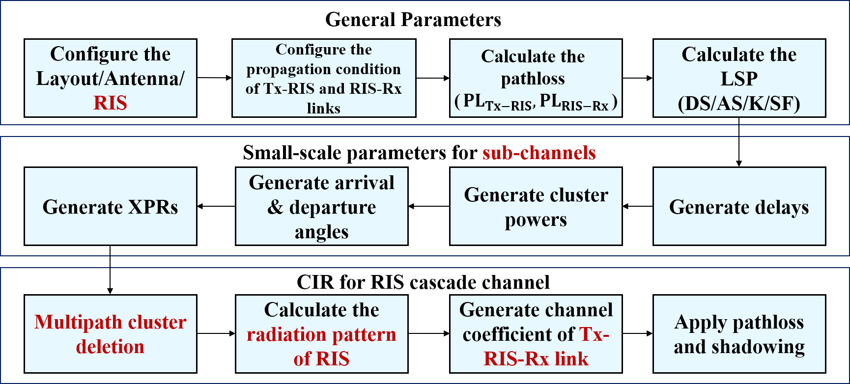
Figure 24: RIS cascade channel model implementation framework[208].

The implementation of the proposed model is based on the 3GPP standardized channel model with some improvements. Fig. 24 illustrates the modeling framework, which consists of three parts: 1) General Parameters, 2) Small-scale parameters, and 3) CIR. The model generates LSPs and SSPs for both Tx-RIS and RIS-Rx sub-channels. The radiation pattern of the RIS is calculated using a method proposed in [204] to account for the angle-dependent characteristics of the RIS phase modulation. For further details on the specific implementation processes, readers may refer to [208].

The existing RIS channel modeling methods can be broadly categorized into statistical methods [211, 205], deterministic methods [204, 212], and hybrid channel models [213], in addition to the previously discussed GBSM-based method. These methods differ in their trade-offs between model accuracy and complexity. Statistical methods generally have lower model complexity but may sacrifice some accuracy, while deterministic methods tend to provide higher accuracy but come with higher computational complexity. Hybrid models aim to strike a balance between the two, leveraging the advantages of both approaches.

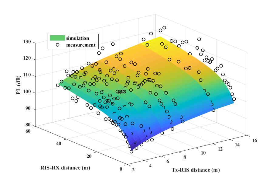
Figure 25: PL result of measurement and simulation [204]. The discrete points refer to measured PL of RIS channel in [197], and continuous surfaces refer to simulation PL result with proposed RIS model in [204].

In [211], a RIS-assisted communication channel modeling method for the sub-6 GHz band is proposed based on the 3GPP standards, and related work is extended to multiple RIS cases in [205]. In [204], the authors use impedance boundary conditions and equivalent impedance to derive the relationship between the reflection coefficient of the RIS element and the incident angle and combine the physical optics method and ray tracing method to achieve the deterministic channel modeling of RIS. The path loss measurement activities are carried out in the corridor scenario, and as shown in Fig. 25, the simulation results of this method are highly matched with the measured data. Different from the above cluster-based modeling methods, [212] introduces a circuit-based communication model for RIS-assisted wireless systems. This model takes into account the mutual impedance between all radiation elements (transceiver antenna, RIS element), and introduces RIS into the communication model by introducing the influence of RIS on the equivalent current and equivalent voltage of the transceiver antenna. The authors in [213] propose a RIS channel modeling method based on a map-based hybrid channel model (MHCM). In this study, the multipath information in complex scenes is generated by ray tracing method, and the RIS surface is modeled as a virtual base station excited by different incoming waves. The gain of RIS for different multipath is calculated, and finally, the channel coefficients of the entire RIS channel are generated by multipath merging.

VI-D Summary and Prospect

The RIS channel measurement is mainly aimed at measuring path loss. The characteristics of RIS channels mainly include the RIS response characteristics and the changes in traditional channel characteristics after the introduction of RIS. The RIS response characteristics include the reflection coefficient characteristics, RIS element radiation pattern, and RIS overall radiation pattern. The path loss characteristics of the RIS channel have significant changes compared to traditional models. In addition, there are also near-field effects and spatial non-stationary characteristics in the RIS channel. These characteristics are worth considering in RIS channel modeling. Based on a comprehensive analysis of these studies, we can foresee some challenges that RIS research may encounter.

VI-D1 RIS channel measurement

RIS channel measurement is an important method for studying RIS channel characteristics and establishing and verifying the RIS channel model. However, due to the high transmission loss of the RIS-assisted channel caused by the Tx-RIS-Rx cascade link, puts forward a higher demand on the transmission power and dynamic range of the measurement platform. In addition, the measurement platform needs a complete architecture such as multi-channel, high sampling rate, and transmit-receive separation to acquire channel characteristics of various complex scenarios.

VI-D2 RIS response characteristics

The reflection coefficient characteristic is an important RIS response characteristic. To characterize the reflection coefficient characteristic of the RIS element, several RIS hardware models have been described above. However, the hardware implementations of RIS are diverse, thus, not all of them can be included in these models. Considering that it is too expensive to build a hardware model for each type of RIS, it is a big challenge to propose an accurate and universal RIS hardware model in the future.

VI-D3 RIS channel modeling

Some literature on RIS channel modeling involving near-field and non-stationary characteristics is presented above. Predictably, continuous attention needs to be paid to channel modeling for RIS-assisted communication in the near field and non-stationary cases, due to RIS with a large area being required to achieve significant channel gain in many scenarios because of the passive nature of RIS. In addition, RIS is similar to a radiation source, each incident multipath will excite the radiation of RIS once, and each radiation of RIS will reach Rx through multiple paths, which will cause a large increase in the number of multipaths. This brings a high computational challenge.

VII 6G Channel Simulation Platform

In this section, the 6G channel simulator called Beijing University of Posts and Telecommunication’s Channel Model Generator-IMT2030 (BUPTCMG-IMT2030) is introduced, which is developed by ARTT Lab of BUPT. We briefly introduce the history, software structure, and functions of BUPTCMG-IMT2030. Then a tutorial of simulations in typical 6G application scenarios using BUPTCMG-IMT2030 is given, including configurations, simulation results, and simple analysis for each given scenario.

VII-A Introduction of BUPTCMG-IMT2030

Implementation and simulation of wireless channel models are increasingly important for designing communication systems. As major auxiliary tools, channel model simulators play significant roles in performance evaluation and network deployment of communication systems.

In recent years, several channel simulators have been developed and used widely. In 2017, New York University (NYU) released a channel simulator named NYUSIM [214], which was developed based on the statistical spatial channel models proposed by NYU. At the newest version of 4.0 launched in 2023, NYUSIM supports the simulation of various scenarios, like InH, InF, UMa, UMi, and RMa, from 0.5 to 150 GHz with spatial consistency, human blockage, and other features. In 2014, Quasi Deterministic Radio Channel Generator (QuaDriGa) was released by Fraunhofer Heinrich-Hertz-Institute [215]. QuaDriGa is a powerful wireless channel simulator that supports various wireless channel models, scenarios, and techniques including Orthogonal Frequency Division Multiplexing (OFDM), multi-input multi-output (MIMO), Single-carrier Frequency-Division Multiple Access (SC-FDMA), etc. In 2018, IMT-2020 CM-BUPT [216] was launched as a MATLAB implementation of the widely recognized standardized channel models defined in ITU-R M.2412 [217], 3GPP TR36.873 [218], 3GPP TR38.900 [219] and 3GPP TR38.901 [121]. Based on the standardized GBSM model described in the documentation above (hereafter referred to as ”standardized model”), IMT-2020 CM-BUPT offers a solution for simulating and analyzing communication channels in scenarios like UMi, UMa, InH, and so on. On December 29, 2022, based on the research in [220], the ARTT team developed and released the RIS-asisted channel simulator named BUPTCMG-IMT2030-RIS which has the ability to simulate a channel where a RIS serves as a relay.

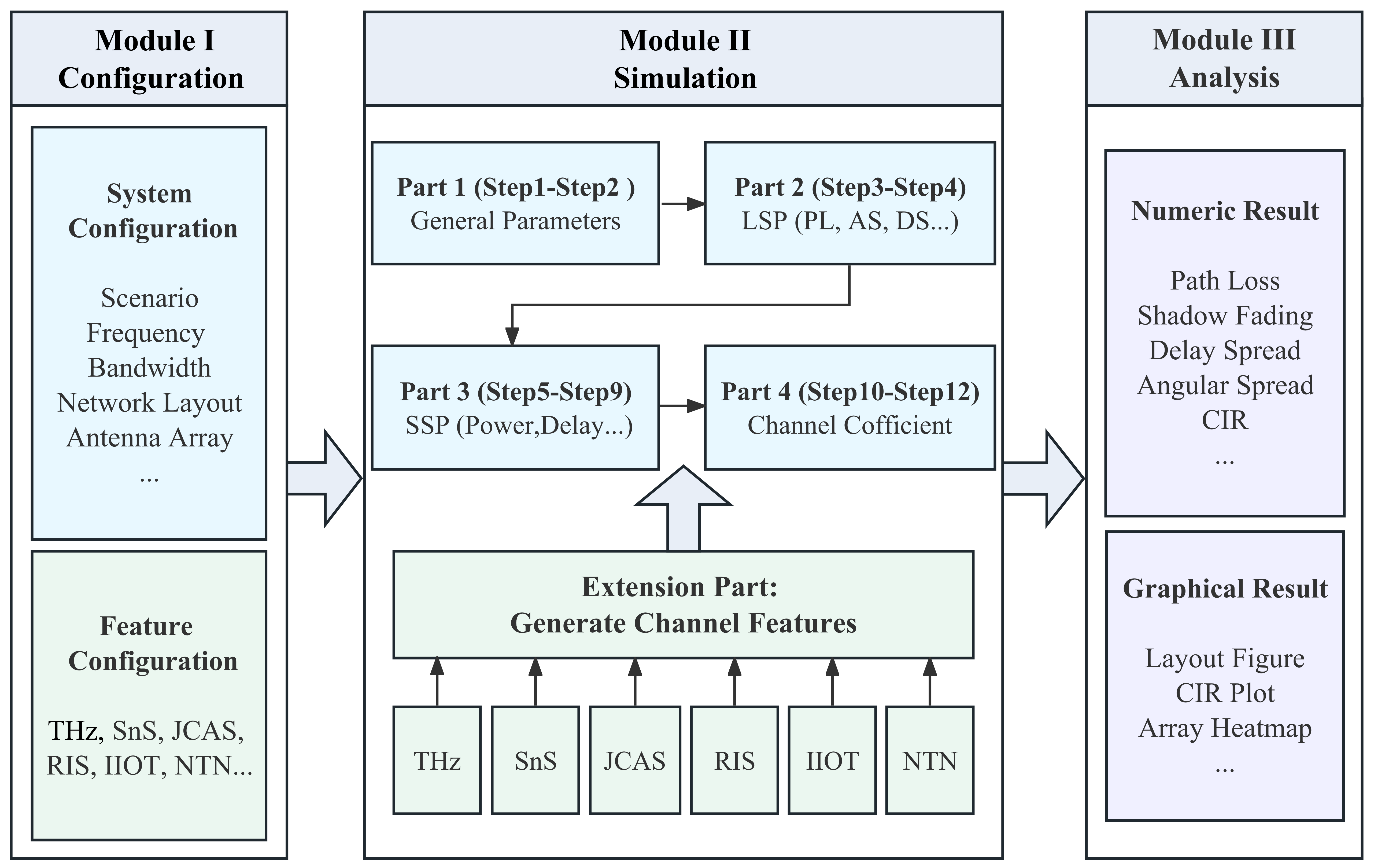
(a) Simulation procedure of 6G channel model (BUPTCMG-IMT2030).

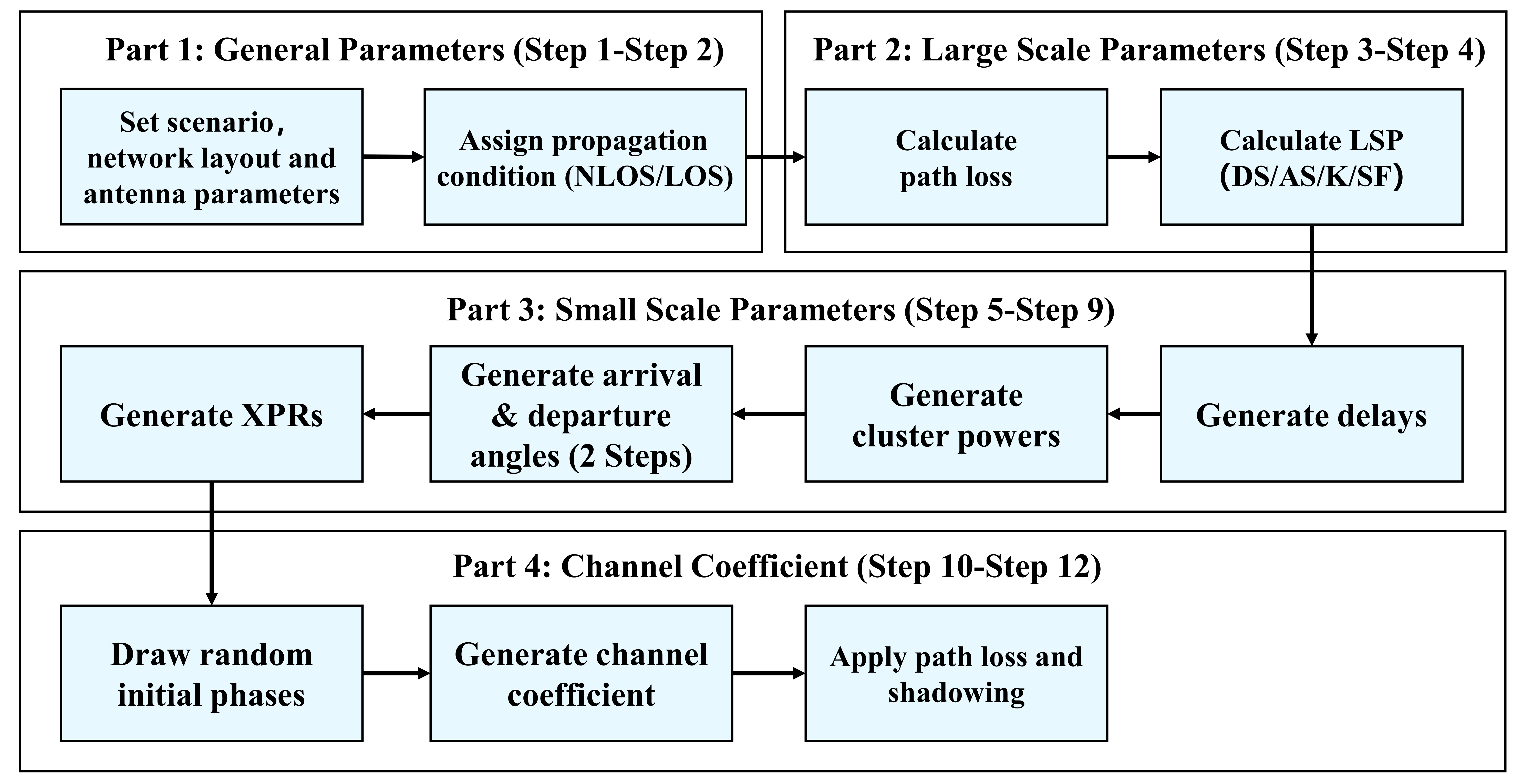
(b) Simulation procedure of 5G ITU/3GPP channel model.

Figure 26: Software structure of 6G channel model (BUPTCMG-IMT2030).

With the fast development of research for 6G communication techniques and features, the requirements for channel simulation for new frequency bands, new channel characteristics, and new propagation mechanisms also increase fastly. To fill the blank of simulations for 6G technologies and new features and meet the requirements of research and development of 6G wireless communications, the ARTT team extended the standardized channel model framework using models proposed in various channel measurement campaigns and developed a 6G channel simulator called BUPTCMG-IMT2030 based on the existing IMT-2020 CM-BUPT and BUPTCMG-IMT2030-RIS.

VII-B Software structure and functions

BUPTCMG-IMT2030 is implemented in MATLAB using a procedure-oriented framework. The software structure is illustrated in Fig. 26. The software is mainly divided into three modules: Configuration, Simulation, and Analysis. In Module I, the configuration module, system parameters like scenario, center frequency, bandwidth, and others will be defined. Next in Module II, the simulation module, BUPTCMG-IMT2030 performs a simulation and generates a series of channel parameters using configurations defined in Module I. Finally in Module III, the analysis module, simulation results are simply analyzed and shown in both numerical and graphical formats. A step-wise description of the simulation is given as follows, including the main functions and extensions for 6G channel technologies and features of BUPTCMG-IMT2030.

VII-B1 Module I: Configuration

In the configuration module, the simulation parameters will be defined. There are two types of configurations, including System Configurations and Feature Configurations, in BUPTCMG-IMT2030. System Configurations include configurations and parameters necessary for a complete simulation, including the scenario, center frequency, bandwidth, positions of BS and UT, antenna type and layout, mobility of UT, and so on. Feature Configurations are extensions for channel features, including the type of features and parameters necessary for this type of feature. In BUPTCMG-IMT2030, various of 6G channel features are supported and can be added to the standardized model, including parameter extensions and sparsity simulation for THz channel, the SnS feature for MIMO channel, and other features for channels like JCAS channel and RIS-Assisted channel. After both two types of configurations are completed, all the configurations and parameters will be saved in a file and the simulator is ready for the channel generation.

VII-B2 Module II: Simulation

In the simulation module, BUPTCMG-IMT2030 performs a simulation according to configurations in Module I. A step-to-step description of the simulation, which can be referred in Fig. 26, is given below.

• Part 1: Generate General Parameters

  This part is used for generating general parameters like network layout, propagation condition, and so on, mentioned in Step 1 and Step 2 of the standardized model in [121], which are decided based on parameters configured by users. Firstly, positions of BS and UT are decided. The 2D location of BS is fixed at the origin of the Cartesian coordinate system, and the height of BS is decided according to scenario parameters defined in [121]. Then the location of UT is dropped manually or randomly, based on the choice of users. Next positions of antenna arrays are decided according to positions of BS and UT (reference points of antenna arrays are set on BS and UT positions). After that, based on positions of UT and BS, the distance between BS and UT, and the LOS angle are calculated. Finally the propagation condition(indoor or outdoor, LOS or NLOS) is decided based on the choice of users or models defined in [121].

• Part 2: Generate Large-Scale Parameters

  This part is used for generating path loss and Large-Scale distribution parameters mentioned in Step 3 and Step 4 of the standardized model in [121]. Based on the scenario, distance, and propagation condition in Part 1, path loss between BS and UT will be calculated. Besides, large-scale parameters, including delay spread (DS), azimuth and zenith angular spread (ASA, ASD, ZSA, ZSD), Ricean K factor (K), and shadow fading (SF), will be randomly generated according to the method described in [121].

• Part 3: Generate Small-Scale Parameters

  This part is used for generating the Small-Scale parameters mentioned in Step 5 to Step 9 of the standardized model in [121]. In Part 2, a series of Large-Scale parameters are generated, and they are used to generate the delay, power, azimuth (or zenith) angles of arriving and departure angles (AOA, AOD, ZOA, ZOD) and the cross-polarization power ratios (XPR) of each cluster and ray. Firstly, the delay and power of clusters are calculated using the delay spread generated before. Delays of rays within a cluster are considered the same as that of the cluster, and the power of the cluster is divided equally and assigned to each ray. Then angles of clusters are generated based on delay, power, and angle spreads generated before. Next, angles of rays are calculated by adding offsets to cluster angles. Finally, the XPR of each ray is generated and the distribution parameters can be found in the parameter table in [121].

• Part 4: Calculate Channel Coefficients

  This part is used for generating Channel Coefficients mentioned in Step 10 to Step 12 in the standardized model in [121]. All the necessary parameters of the simulated channel are generated in previous parts except the random initial phases of each ray, which are generated in this part. At first, the Channel Coefficients of each ray is calculated using the power, angle, phase, and other parameters. Then coefficients of rays within a cluster are joined together to get the cluster coefficients, which are considered as the Channel Impulse Response (CIR) of the channel. After that, the simulator generates the Channel Frequency Response (CFR) of the channel using the cluster CIRs. Formulas and parameters of this calculation can be found in [121].

• Extension Part: Generate 6G Channel Features

  According to configurations, some extra parts may be added between parts above, in most situations between Part 3 and Part 4. The extensions supported by BUPTCMG-IMT2030 are described below:

  Extensions for THz Frequency Band. BUPTCMG-IMT2030 has extended the parameters in standards, which only support frequency in the range of 0.5-100 GHz, to the THz Frequency Band. In the extended parameter table, simulation for 100 GHz and 132 GHz is supported. It is noticed that compared to the channel simulation steps described in [121], THz simulation changes some steps due to its sparse characteristics for clusters and rays. To simulate the sparsity of the channel in the THz frequency band, a model used to introduce sparsity using the parameter intra-cluster K-factor (ICK) described in [221] is implemented and used.

  Extensions for Spatial Non-Stationary. BUPTCMG-IMT2030 supports simulations for spatial non-stationary characteristics of MIMO channels, including both the visibility change on the antenna array and the phase characteristics of the spherical wave-front according to [157]. The implementation includes two parts. In the first part, simulation for the visibility of each cluster is implemented based on a two-state Markov chain. In the second part, positions of the first-bounce scatter (FBS) and last-bounce scatter (LBS) are estimated according to delays and angles of rays, and the phase evolution of spherical wave-front is calculated based on the distance between BS elements and FBS, UT elements and LBS.

  Extensions for JCAS. The cluster-based statistical channel model for researching JCAS channel characteristics is implemented in BUPTCMG-I2030. To simulate a JCAS channel, parameters for JCAS extension are necessary, including the layout of sensing targets, the RCS, the shared cluster number, and others. The simulator uses these configurations to generate the sensing target channel and correct the shared cluster parameters (such as cluster delay and angle), as well as realize the traditional communication channel. Finally, a communication channel and a sensing channel with sharing feature can be generated, respectively.

  Extensions for RIS. Supports for RIS-assisted channel implemented in BUPTCMG-IMT2030-RIS simulator are integrated into BUPTCMG-IMT2030, offering simulations of RIS-assisted channel. To perform a RIS-assisted channel, configurations of RIS in Module I are needed, including RIS position, RIS size, and element layout, and a user-defined code book. The RIS serves as a relay between BS and UT [220], so channel parameters of RIS-assisted channel is divided into three parts, channel between BS ans UT, BS ans RIS, RIS and UT. After configuring parameters needed, BUPTCMG-IMT2030 generates channel parameters and channel coefficients of the three parts and calculates cascade channel coefficients of the RIS-assisted channel.

  Extensions for Industrial IOT (IIOT). In BUPTCMG-IMT2030, simulation for IIOT Scenario is supported. To perform simulation in the IIOT scenario, parameters of the scenario, including the room size, clutter density, clutter size and others, are needed in Module I. Different configurations leads to different scenario Type (e.g. sparse or dense clutter, low BS or high BS) and different simulation parameters. The Generation follows the same procedure as standard model in Module II.

  Extensions for Non-Terrestrial Network (NTN). Supports for NTN channel simulation is implemented in BUPTCMG-IMT2030. In NTN Scenario, BS is set on a satellite, and the position of BS and UT is defined using latitude, longitude and height. The Generation follows the same procedure as standard model in Module II, but the parameter of simulation varies with the change of elevation angle and relative position of BS and UT.

TABLE V: Configurations for Simulation Examples

6G Cases	System Configurations	Channel Feature Configurations
THz	Scenario: UMi-Street Canyon; LOS Status: LOS Center Frequency: 132 GHz; Bandwidth: 1.2 GHz Position (x,y,z): BS:[0,0,3] (m); UT:[10,10,3] (m) Antenna: BS: Single Antenna; UT: Single Antenna	Intra-Cluster K-Factor: 17.98
SnS	Scenario: UMi-Street Canyon; LOS Status: LOS Center Frequency: 28 GHz; Bandwidth: 200 MHz Position (x,y,z): BS:[0,0,3] (m); UT:[10,10,3] (m) Antenna: BS: 256-Element ULA; UT: Single Antenna	Stationary Region Size: 16 Elements
JCAS	Scenario: Indoor-Hospot; LOS Status: LOS Center Frequency: 28 GHz; Bandwidth: 200 MHz Position (x,y,z): BS:[0,0,1.5] (m); UT:[10,0,1.5] (m) Antenna: BS: Single Antenna; UT: Single Antenna	Number of Sensing Targets: 3 Number of Sensing Clusters: 1 Echo Path Loss: Free Space Radar Path Loss RCS Parameters: fixed Method of JCAS: Shared Cluster
RIS	Scenario: UMi-Street Canyon; LOS Status: LOS Center Frequency: 28 GHz; Bandwidth: 200 MHz Position (x,y,z): BS:[0,0,3] (m); UT:[10,10,3] (m) Antenna: BS: Single Antenna; UT: Single Antenna	RIS Position: [5,20,3] RIS Size: 32*32 elements Code Book: Continuous anomalous reflection

VII-B3 Module III: Analysis

After the Simulation, series channel parameters are generated, and BUPTCMG-IMT2030 performs a simple analysis of the channel. BUPTCMG-IMT2030 calculates the Delay Spread (DS), Angular Spreads (ASA, ASD, ZSA, ZSD), Reference Signal Receive Power (RSRP), Gini index (used for sparsity analysis) and so on according to parameters and channel coefficients generated. Then, a simple overview of the simulation is given as a Graphical User Interface, including numeric results and some graphical results like Network Layout, CIR of a single link, and others. After that, all the results will be integrated together and saved as in files in a path that users defined.

VII-C Applications

In this section, results for typical 6G channel simulations are described, including 6G new frequency band (THz), new channel characteristic (SnS), and new propagation mechanism (JCAS and RIS). Configurations of each scenario are given in Table V, detailed input parameters and output parameters can be found in the User Manuel of BUPTCMG-IMT2030.

VII-C1 6G Case 1: New Frequency-THz Frequency Fand

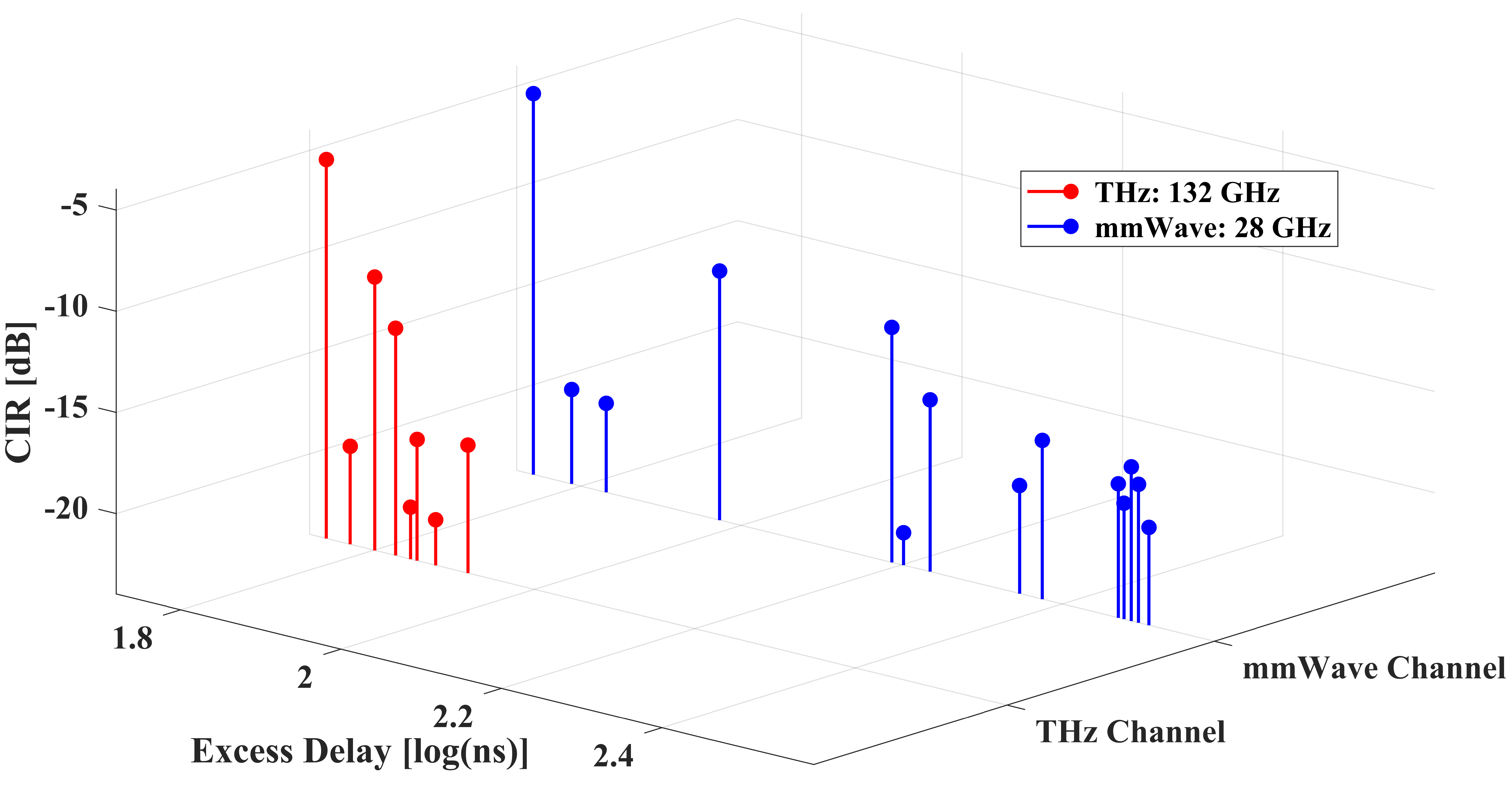
Figure 27: Simulation results for THz channel CIR.

Using configurations in Table V, a simulation for the channel in the THz Frequency band(hereinafter referred to as THz channel) is performed, and results compared with a channel in the mmWave Frequency band(hereinafter referred to as mmWave channel) are displayed in Fig. 27, which is a CIR plot of two channels. Configurations of two channels are same except the center frequency, which is 132 GHz in THz channel and 28 GHz in mmWave channel. As is shown in Fig. 27, compared with the mmWave channel, fewer multipaths can be found in the THz channel, indicating that the THz channel has a more sparse structure than the mmWave channel does. Besides, the observed multipath is concentrated in a narrower delay range than the mmWave channel, which means that multipath in the THz channel is more concentrated in a small range of time (i.e., the delay spread of the THz channel is smaller than that of the mmWave channel).

VII-C2 6G Case 2: New Channel Characteristic-Spatial Non-Stationary (SnS)

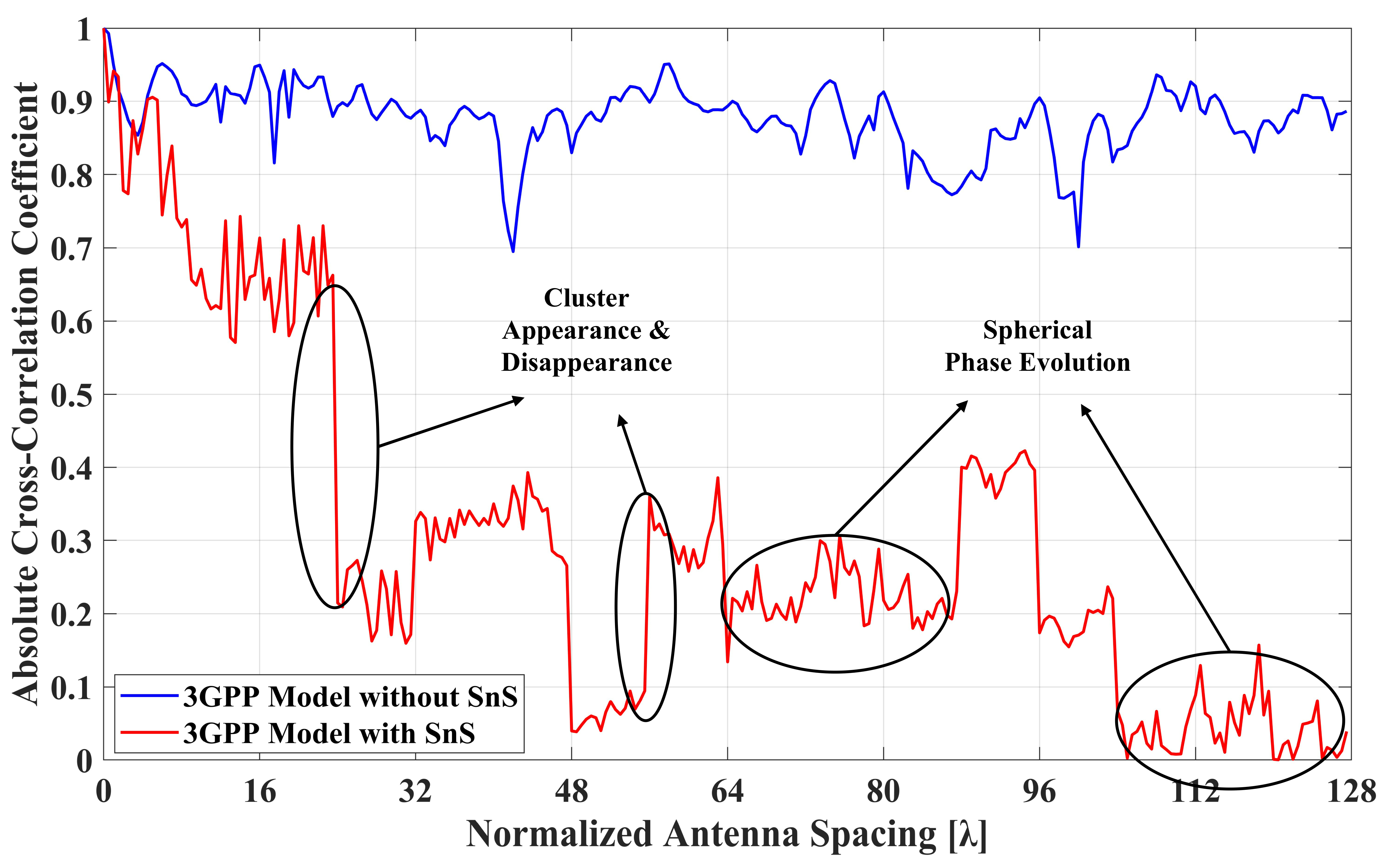
Figure 28: Simulation results for SnS feature.

Using configurations in Table V, a channel in which massive MIMO is configured is generated. As is shown in Table V, a uniform linear array (ULA) with 256 antenna elements is used in BS and a single antenna is used in UT. The result is shown in Fig. 28, which is the absolute cross-correlation coefficients of CIR between the reference element and other elements. It can be found that there are two curves in Fig. 28, one is the channel using models with SnS(hereinafter referred to as SnS channel) and the other is the channel using the standardized model(hereinafter referred to as standardized channel). According to Fig. 28, with the increase of spacing between two elements, the cross-correlation coefficient of the standardized model stays stable at around 0.9, but that of the SnS channel decreases, indicating that the correlation of two elements becomes weaker. Besides, two phenomena, the appearance or disappearance of clusters and the evolution of power and phase, can be found. The appearance or disappearance of clusters results in a sudden change of cross-correlation coefficients, including an increase for the appearance and a decrease for the disappearance, and the evolution of power and phase results in a change of cross-correlation coefficients when no cluster appears or disappears.

VII-C3 6G Case 3: New Propagation Mechanism-JCAS

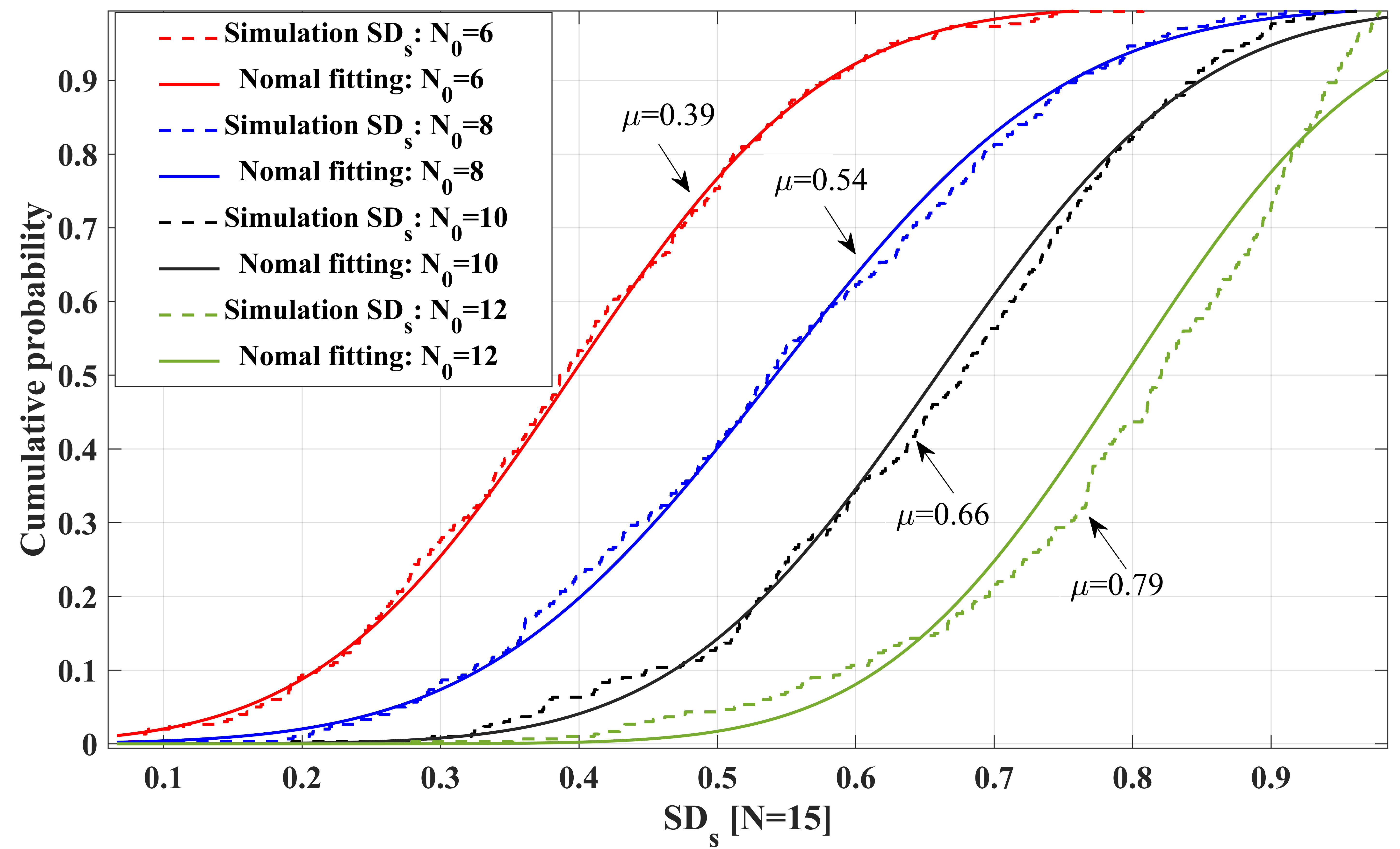
Figure 29: Simulation results for JCAS channel.

To simulate JCAS channel, configurations in Table V can be used, and simulation results are shown in Fig. 29. In the JCAS system, the sharing degree (SD) is used to measure the power ratio of the shared clusters in the JCAS channels. When SD becomes higher, the potential to realize the mutual auxiliary functions of communication and sensing becomes greater. Fig. 29 is cumulative distribution functions (CDF) of SD metric in sensing channels (SDs) under the different number of shared clusters N0. It can be found that the larger $N_{0}$ is, the higher SDs become, which is validated in measurement results. The desired SDs value can be obtained by controlling the appropriate parameters of the proposed channel model, enabling the flexible simulation of JCAS channels.

VII-C4 6G Case 4: New Propagation Mechanism-RIS

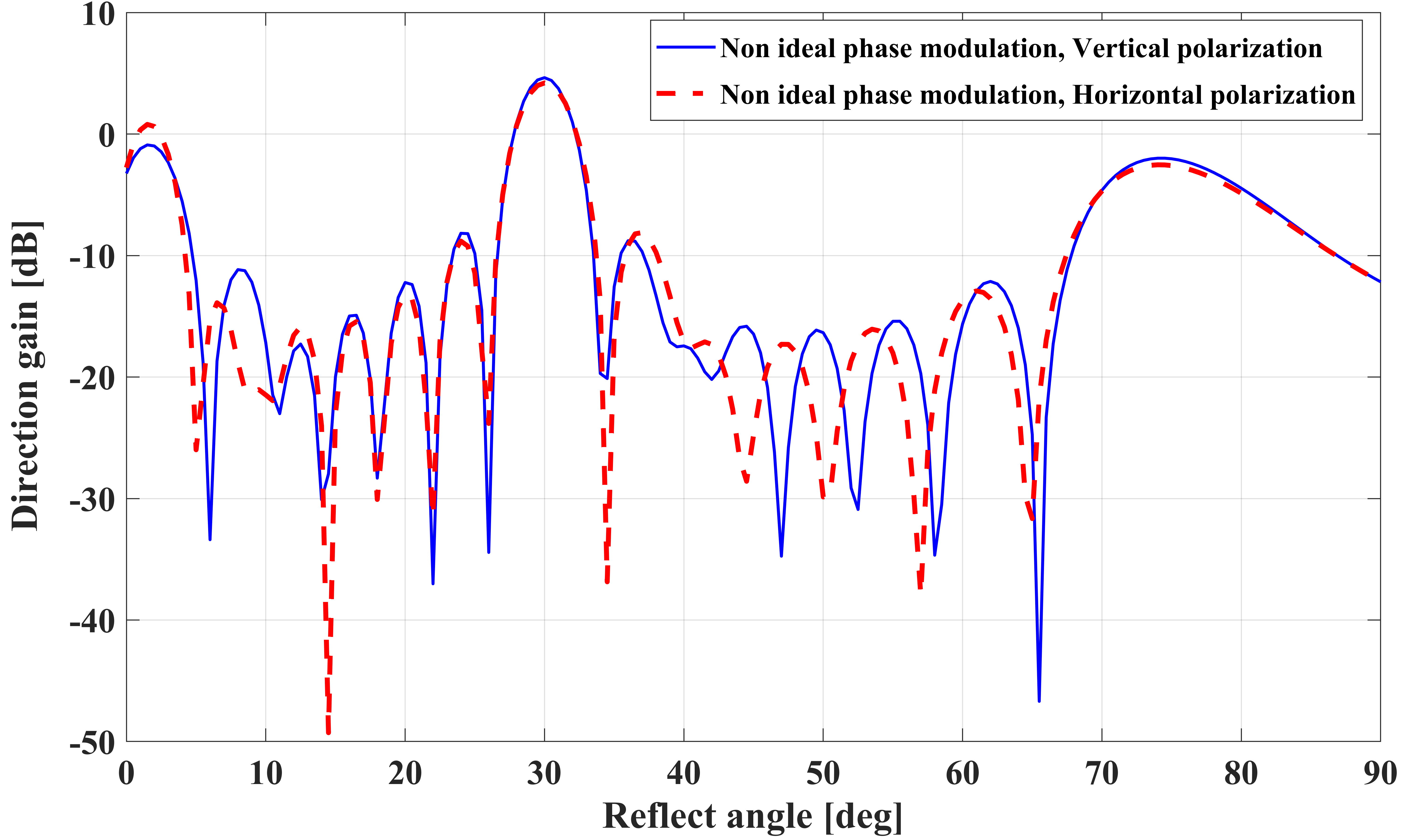
Figure 30: Simulation results for RIS-assisted channel.

To perform a RIS-assisted channel simulation, users need to configure the RIS configuration, including size, code book, area of the elements, direction, and so on, in Module I as shown in Table V. Simulation results of the RIS-Assisted channel are shown in Fig. 30, which is the radiation pattern of RIS with different polarization components. It can be found that one path arrives at RIS with ZOA of $30^{\circ}$. The operating regime is set to continuous anomalous reflection. With this operation strategy, each element of the RIS is continuous phase modulated so that the target beam is oriented towards ZOD of $\theta_{target}$. Fig. 30 shows that the radiation pattern of RIS is also affected by the polarization of the incident path.

VII-D Summary and Prospect

In this section, a channel model simulator called BUPTCMG-IMT2030 is introduced, including its predecessors such as IMT2020-BUPT-CM and BUPTCMG-IMT2030-RIS, software structure, application examples, and simulation results for typical 6G techniques. To summarize, BUPTCMG-IMT2030 is a link-level channel model simulator developed for 6G wireless communication by the ARTT team of BUPT. In the current version, BUPTCMG-IMT2030 supports simulations for standardized channel model defined in ITU-R M.2412 and adds a series of extensions for 6G features and technologies such as Extension of Frequency Band to THz, SnS, JCAS, RIS, and so on. In future versions, more channel models and implementations, like Non-terrestrial Networks, Industrial Internet of Things (IIOT), and others, will be added and make BUPTCMG-IMT2030 a powerful assistance tool for channel model simulation.

VIII Conclusion

In this paper, a survey of 6G channel research and a tutorial on the 6G channel simulation platform are presented. The principle of ITU standard channel modeling and the four challenges faced by 6G channel modeling, including higher frequency band, extremely large antenna array, new technology combinations, and more diverse scenarios. Channel measurement and modeling of promising key technologies in 6G, including THz, massive MIMO, JCAS, and RIS, are reviewed and prospected. So far, the research on channel measurement and modeling still needs further exploration to support the design and application of the 6G communication system. First, for channel measurement, a measurement platform with high accuracy and supporting multiple scenarios is an urgent need to meet the development needs. Second, for channel modeling, near-field effects, and non-stationary characteristics are required to be properly included in THz, massive MIMO, and RIS channel model. Shared scatterers, target modeling, and clutter modeling, which are derived by JCAS in combination with non-communication sensing techniques, also need to be considered. Finally, geometry based stochastic modeling is one of the main modeling methods of 6G, but the model needs to be adjusted under different technologies and scenarios. We implement and guide the ITU/3GPP 6G channel simulator, BUPTCMG-IMT2030. The channel simulation platform has good backward compatibility and is expected to include more modeling techniques and scenarios in the future.

References

- [1] ITU, “Future technology trends of terrestrial International Mobile Telecommunications systems towards 2030 and beyond,” ITU-R M.2516, Nov. 2022.
- [2] ITU, “IMT Vision–Framework and overall objectives of the future development of IMT for 2030 and beyond,” ITU-R M.[IMT.VISION 2030 AND BEYOND.
- [3] ITU, “IMT Traffic estimates for the years 2020 to 2030,” ITU-R M. 2370, July 2015.
- [4] https://www.ericsson.com/en/mobility-report/reports/june-2020/.
- [5] W. Jiang, B. Han, M. A. Habibi, and H. D. Schotten, “The Road Towards 6G: A Comprehensive Survey,” IEEE Open Journal of the Communications Society, vol. 2, pp. 334–366, 2021.
- [6] Z. Hu, J. Zhang, K. Niu, G. Nie, H. Tian, Q. Qi, and Z. Ding, “Ubiquitous-X: Constructing the Future 6G Networks,” SCIENTIA SINICA Informationis, vol. 50, p. 913, 06 2020.
- [7] C. Wang, J. Huang, H. Wang, X. Gao, X. You, and Y. Hao, “6G Wireless Channel Measurements and Models: Trends and Challenges,” IEEE Vehicular Technology Magazine, vol. 15, no. 4, pp. 22–32, 2020.
- [8] B. Ji, Y. Han, S. Liu, F. Tao, G. Zhang, Z. Fu, and C. Li, “Several Key Technologies for 6G: Challenges and Opportunities,” IEEE Communications Standards Magazine, vol. 5, no. 2, pp. 44–51, 2021.
- [9] S. Rajoria and K. Mishra, “A brief survey on 6G communications,” Wireless Networks, vol. 28, pp. 2901–2911, 2022.
- [10] W. Saad, M. Bennis, and M. Chen, “A Vision of 6G Wireless Systems: Applications, Trends, Technologies, and Open Research Problems,” IEEE Network, vol. 34, no. 3, pp. 134–142, 2020.
- [11] M. Giordani, M. Polese, M. Mezzavilla, S. Rangan, and M. Zorzi, “Toward 6G Networks: Use Cases and Technologies,” IEEE Communications Magazine, vol. 58, no. 3, pp. 55–61, 2020.
- [12] J. Zhang, P. Tang, L. Yu, T. Jiang, and L. Tian, “Channel measurements and models for 6G: current status and future outlook,” Frontiers of Information Technology & Electronic Engineering, vol. 21, pp. 39–61, 2020.
- [13] P. Tang, J. Zhang, H. Tian, Z. Chang, J. Men, Y. Zhang, L. Tian, L. Xia, Q. Wang, and J. He, “Channel measurement and path loss modeling from 220 GHz to 330 GHz for 6G wireless communications,” China Communications, vol. 18, no. 5, pp. 19–32, 2021.
- [14] J. Zhang, J. Lin, P. Tang, W. Fan, Z. Yuan, X. Liu, H. Xu, Y. Lyu, L. Tian, and P. Zhang, “Deterministic Ray Tracing: A Promising Approach to THz Channel Modeling in 6G Deployment Scenarios,” IEEE Communications Magazine, 2023.
- [15] P. Zhang, K. Niu, H. Tian, G. Nie, X. Qin, Q. Qi, and J. Zhang, “Technology prospect of 6G mobile communications,” Journal on Communications, vol. 40, no. 1, pp. 141–148, 2019.
- [16] G. Nie, J. Zhang, Y. Zhang, L. Yu, Z. Zhang, Y. Sun, L. Tian, Q. Wang, and L. Xia, “A predictive 6G network with environment sensing enhancement: From radio wave propagation perspective,” China Communications, vol. 19, no. 6, pp. 105–122, 2022.
- [17] T. Mao, J. Chen, Q. Wang, C. Han, Z. Wang, and G. K. Karagiannidis, “Waveform Design for Joint Sensing and Communications in Millimeter-Wave and Low Terahertz Bands,” IEEE Transactions on Communications, vol. 70, no. 10, pp. 7023–7039, 2022.
- [18] J. Wang, N. Varshney, C. Gentile, S. Blandino, J. Chuang, and N. Golmie, “Integrated Sensing and Communication: Enabling Techniques, Applications, Tools and Data Sets, Standardization, and Future Directions,” IEEE Internet of Things Journal, vol. 9, no. 23, pp. 23416–23440, 2022.
- [19] F. Liu, Y. Cui, C. Masouros, J. Xu, T. X. Han, Y. C. Eldar, and S. Buzzi, “Integrated Sensing and Communications: Toward Dual-Functional Wireless Networks for 6G and Beyond,” IEEE Journal on Selected Areas in Communications, vol. 40, no. 6, pp. 1728–1767, 2022.
- [20] L. Zhang, X. Q. Chen, and T. Jun Cui, “Space-Time-Coding Digital Metasurfaces for Multiplexed Wireless Communications,” in 2021 International Conference on Microwave and Millimeter Wave Technology (ICMMT), pp. 1–3, 2021.
- [21] T. J. Cui, M. Q. Qi, X. Wan, J. Zhao, and Q. Cheng, “Coding metamaterials, digital metamaterials and programmable metamaterials,” Light: science & applications, vol. 3, no. 10, pp. e218–e218, 2014.
- [22] J. Liu, Y. Shi, Z. M. Fadlullah, and N. Kato, “Space-Air-Ground Integrated Network: A Survey,” IEEE Communications Surveys & Tutorials, vol. 20, no. 4, pp. 2714–2741, 2018.
- [23] H. Jiang, M. Mukherjee, J. Zhou, and J. Lloret, “Channel Modeling and Characteristics for 6G Wireless Communications,” IEEE Network, vol. 35, no. 1, pp. 296–303, 2021.
- [24] K. M. Saidul Huq, J. Rodriguez, I. E. Otung, and S. Stavrou, “Recent Advances of Propagation Channel Research for 6G Wireless Communication Systems,” in 2021 IEEE Globecom Workshops (GC Wkshps), pp. 1–6, 2021.
- [25] ITU, “Guidelines for evaluation of radio interface technologies for IMT-2020,” ITU-R M.2412, Oct. 2017.
- [26] 3GPP, “Study on channel model for frequencies from 0.5 to 100 GHz (Release 15),” tech. rep., 3GPP TR 38.901, 2018.
- [27] C.-L. Cheng, S. Kim, and A. Zajić, “Comparison of path loss models for indoor 30 GHz, 140 GHz, and 300 GHz channels,” in 2017 11th European Conference on Antennas and Propagation (EUCAP), pp. 716–720, IEEE, 2017.
- [28] G. R. MacCartney, J. Zhang, S. Nie, and T. S. Rappaport, “Path loss models for 5G millimeter wave propagation channels in urban microcells,” in 2013 IEEE Global Communications Conference (GLOBECOM), pp. 3948–3953, IEEE, 2013.
- [29] S. Sun, G. R. MacCartney, and T. S. Rappaport, “Millimeter-wave distance-dependent large-scale propagation measurements and path loss models for outdoor and indoor 5G systems,” in 2016 10th European Conference on Antennas and Propagation (EuCAP), pp. 1–5, IEEE, 2016.
- [30] G. R. Maccartney, T. S. Rappaport, S. Sun, and S. Deng, “Indoor office wideband millimeter-wave propagation measurements and channel models at 28 and 73 GHz for ultra-dense 5G wireless networks,” IEEE Access, vol. 3, pp. 2388–2424, 2015.
- [31] S. Sun, T. S. Rappaport, S. Rangan, T. A. Thomas, A. Ghosh, I. Z. Kovacs, I. Rodriguez, O. Koymen, A. Partyka, and J. Jarvelainen, “Propagation path loss models for 5G urban micro-and macro-cellular scenarios,” in 2016 IEEE 83rd Vehicular Technology Conference (VTC Spring), pp. 1–6, IEEE, 2016.
- [32] J. Zhang, Y. Zhang, Y. Yu, R. Xu, Q. Zheng, and P. Zhang, “3-D MIMO: How Much Does It Meet Our Expectations Observed From Channel Measurements?,” IEEE Journal on Selected Areas in Communications, vol. 35, no. 8, pp. 1887–1903, 2017.
- [33] Z. Bao, Z. Nie, and X. Zong, “A novel broadband dual-polarization antenna utilizing strong mutual coupling,” IEEE Transactions on Antennas and Propagation, vol. 62, no. 1, pp. 450–454, 2013.
- [34] A. F. Molisch, Wireless communications, vol. 34. John Wiley & Sons, 2012.
- [35] P. Tang, J. Zhang, A. F. Molisch, P. J. Smith, M. Shafi, and L. Tian, “Estimation of the k-factor for temporal fading from single-snapshot wideband measurements,” IEEE Transactions on Vehicular Technology, vol. 68, no. 1, pp. 49–63, 2018.
- [36] W. R. Conference, “Radio Regulations, Edition of 2019,” tech. rep.
- [37] I.-R. F.2416-0, “Technical and operational characteristics and applications of the point-to-point fixed service applications operating in the frequency band 275-450 GHz,” working paper, 2019.
- [38] F. C. Commission, “First Report and Order.” Online, Mar. 2019. Docket 18-21.
- [39] J. M. of Information and Communication, “ Japan Allocation Table Footnote J36.” Online, 2015.
- [40] J. M. of Information and Communication, “Frequency Allocation Table.” Online, 2020.
- [41] E. C. of Postal, T. A. (CEPT), and the European Radiocommunications Committee (ERC), “CEPT/ERC ERC Recommendation70-03.” Online, Oct. 2018.
- [42] T. Kürner, D. M. Mittleman, and T. Nagatsuma, THz Communications: Paving the Way Towards Wireless Tbps. Springer, 2022.
- [43] Z. Chang, J. Zhang, P. Tang, L. Tian, L. Yu, G. Liu, and L. Xia, “Frequency-Angle Two-Dimensional Reflection Coefficient Modeling Based on Terahertz Channel Measurement,” arXiv preprint arXiv:2207.04596, 2022.
- [44] S. Kim, W. T. Khan, A. Zajić, and J. Papapolymerou, “D-band channel measurements and characterization for indoor applications,” IEEE Transactions on Antennas and Propagation, vol. 63, no. 7, pp. 3198–3207, 2015.
- [45] Y. Chen, Y. Li, C. Han, Z. Yu, and G. Wang, “Channel measurement and ray-tracing-statistical hybrid modeling for low-terahertz indoor communications,” IEEE Transactions on Wireless Communications, vol. 20, no. 12, pp. 8163–8176, 2021.
- [46] Z. Yu, Y. Chen, G. Wang, W. Gao, and C. Han, “Wideband channel measurements and temporal-spatial analysis for terahertz indoor communications,” in 2020 IEEE International Conference on Communications Workshops (ICC Workshops), pp. 1–6, IEEE, 2020.
- [47] Y. Chen, C. Han, Z. Yu, and G. Wang, “140 GHz channel measurement and characterization in an office room,” in ICC 2021-IEEE International Conference on Communications, pp. 1–6, IEEE, 2021.
- [48] J. He, Y. Chen, Y. Wang, Z. Yu, and C. Han, “Channel measurement and path-loss Characterization for low-terahertz indoor scenarios,” in 2021 IEEE International Conference on Communications Workshops (ICC Workshops), pp. 1–6, IEEE, 2021.
- [49] Y. Chen, C. Han, Z. Yu, and G. Wang, “Channel Measurement, Characterization and Modeling for Terahertz Indoor Communications Above 200 GHz,” arXiv preprint arXiv:2205.00220, 2022.
- [50] G. Song, Y. Li, J. Jiang, C. Han, Z. Yu, Y. Du, and Z. Wang, “Channel Measurement and Characterization at 140 GHz in a Wireless Data Center,” in GLOBECOM 2022-2022 IEEE Global Communications Conference, pp. 4764–4769, IEEE, 2022.
- [51] Y. Li, G. Wang, G. Song, M. Xu, J. Jiang, and C. Han, “Wideband Channel Measurement and Characterization on a Computer Motherboard,” in 2022 IEEE Globecom Workshops (GC Wkshps), pp. 1040–1045, IEEE, 2022.
- [52] S. L. Nguyen, K. Haneda, J. Järveläinen, A. Karttunen, and J. Putkonen, “Large-scale parameters of spatio-temporal short-range indoor backhaul channels at 140 GHz,” in 2021 IEEE 93rd Vehicular Technology Conference (VTC2021-Spring), pp. 1–6, IEEE, 2021.
- [53] S. L. Nguyen, J. Jarvelainen, A. Karttunen, K. Haneda, and J. Putkonen, “Comparing radio propagation channels between 28 and 140 GHz bands in a shopping mall,” 2018.
- [54] N. A. Abbasi, A. Hariharan, A. M. Nair, and A. F. Molisch, “Channel measurements and path loss modeling for indoor THz communication,” in 2020 14th European conference on antennas and propagation (eucap), pp. 1–5, IEEE, 2020.
- [55] N. A. Abbasi, A. Hariharan, A. M. Nair, A. S. Almaiman, F. B. Rottenberg, A. E. Willner, and A. F. Molisch, “Double directional channel measurements for THz communications in an urban environment,” in ICC 2020-2020 IEEE international conference on communications (ICC), pp. 1–6, IEEE, 2020.
- [56] N. A. Abbasi, J. Gomez-Ponce, D. Burghal, R. Kondaveti, S. Abu-Surra, G. Xu, C. Zhang, and A. F. Molisch, “Double-directional channel measurements for urban THz communications on a linear route,” in 2021 IEEE international conference on communications workshops (ICC workshops), pp. 1–6, IEEE, 2021.
- [57] N. A. Abbasi, J. Gomez-Ponce, S. M. Shaikbepari, S. Rao, R. Kondaveti, S. Abu-Surra, G. Xu, C. Zhang, and A. F. Molisch, “Ultra-wideband double directional channel measurements for thz communications in urban environments,” in ICC 2021-IEEE International Conference on Communications, pp. 1–6, IEEE, 2021.
- [58] N. A. Abbasi, J. Gomez-Ponce, R. Kondaveti, S. M. Shaikbepari, S. Rao, S. Abu-Surra, G. Xu, C. Zhang, and A. F. Molisch, “Thz band channel measurements and statistical modeling for urban d2d environments,” IEEE Transactions on Wireless Communications, 2022.
- [59] J. Gomez-Ponce, N. A. Abbasi, Z. Cheng, and A. F. Molisch, “Directional characteristics of THz outdoor channels-measurement and system performance implications,” in 2021 55th Asilomar Conference on Signals, Systems, and Computers, pp. 658–663, IEEE, 2021.
- [60] N. A. Abbasi, J. Gomez-Ponce, R. Kondaveti, A. Kumar, E. Bhagat, R. N. Rao, S. Abu-Surra, G. Xu, C. Zhang, and A. F. Molisch, “Double-Directional Channel Measurements for Urban THz Microcellular Communications in a Street Canyon,” in ICC 2022-IEEE International Conference on Communications, pp. 2876–2881, IEEE, 2022.
- [61] N. A. Abbasi, A. F. Molisch, and J. C. Zhang, “Measurement of directionally resolved radar cross section of human body for 140 and 220 GHz bands,” in 2020 IEEE Wireless Communications and Networking Conference Workshops (WCNCW), pp. 1–4, IEEE, 2020.
- [62] R. Piesiewicz, R. Geise, M. Jacob, J. Jemai, and T. Kurner, “Indoor channel measurements of point-to-point ultra broadband short range links between 75 GHz and 110 GHz,” in 2008 IEEE Antennas and Propagation Society International Symposium, pp. 1–4, IEEE, 2008.
- [63] S. Ju, Y. Xing, O. Kanhere, and T. S. Rappaport, “Millimeter wave and sub-terahertz spatial statistical channel model for an indoor office building,” IEEE Journal on Selected Areas in Communications, vol. 39, no. 6, pp. 1561–1575, 2021.
- [64] S. Ju, Y. Xing, O. Kanhere, and T. S. Rappaport, “Sub-terahertz channel measurements and characterization in a factory building,” in ICC 2022-IEEE International Conference on Communications, pp. 2882–2887, IEEE, 2022.
- [65] Y. Xing, O. Kanhere, S. Ju, and T. S. Rappaport, “Indoor wireless channel properties at millimeter wave and sub-terahertz frequencies,” in 2019 IEEE Global Communications Conference (GLOBECOM), pp. 1–6, IEEE, 2019.
- [66] Y. Xing and S. Theodore, “PropagationMeasurementsandPathLossModelsfor sub-THz inUrbanMicrocells,” in IEEE International Conference on Communications, 2021.
- [67] S. Ju and T. S. Rappaport, “Sub-terahertz spatial statistical MIMO channel model for urban microcells at 142 GHz,” in 2021 IEEE Global Communications Conference (GLOBECOM), pp. 1–6, IEEE, 2021.
- [68] S. Ju and T. S. Rappaport, “140 GHz urban microcell propagation measurements for spatial consistency modeling,” in ICC 2021-IEEE International Conference on Communications, pp. 1–6, IEEE, 2021.
- [69] Y. Xing, O. Kanhere, S. Ju, and T. S. Rappaport, “Sub-Terahertz Wireless Coverage Analysis at 142 GHz in Urban Microcell,” in ICC 2022-IEEE International Conference on Communications, pp. 3942–3947, IEEE, 2022.
- [70] A. Schultze, W. Keusgen, M. Peter, and T. Eichler, “Observations on the Angular Statistics of the Indoor Sub-THz Radio Channel at 158 GHz,” in 2022 IEEE USNC-URSI Radio Science Meeting (Joint with AP-S Symposium), pp. 9–10, IEEE, 2022.
- [71] N. Khalid and O. B. Akan, “Wideband THz communication channel measurements for 5G indoor wireless networks,” in 2016 IEEE International Conference on Communications (ICC), pp. 1–6, IEEE, 2016.
- [72] N. Khalid, N. A. Abbasi, and O. B. Akan, “Statistical characterization and analysis of low-THz communication channel for 5G Internet of Things,” Nano Communication Networks, vol. 22, p. 100258, 2019.
- [73] S. Kim and A. G. Zajić, “Statistical characterization of 300 GHz propagation on a desktop,” IEEE Transactions on Vehicular Technology, vol. 64, no. 8, pp. 3330–3338, 2014.
- [74] S. Kim and A. Zajić, “Characterization of 300 GHz wireless channel on a computer motherboard,” IEEE Transactions on Antennas and Propagation, vol. 64, no. 12, pp. 5411–5423, 2016.
- [75] C.-L. Cheng and A. Zajić, “Characterization of propagation phenomena relevant for 300 GHz wireless data center links,” IEEE Transactions on Antennas and Propagation, vol. 68, no. 2, pp. 1074–1087, 2019.
- [76] C.-L. Cheng, S. Sangodoyin, and A. Zajić, “THz cluster-based modeling and propagation characterization in a data center environment,” IEEE Access, vol. 8, pp. 56544–56558, 2020.
- [77] C.-L. Cheng, S. Sangodoyin, and A. Zajić, “Terahertz MIMO fading analysis and doppler modeling in a data center environment,” in 2020 14th European Conference on Antennas and Propagation (EuCAP), pp. 1–5, IEEE, 2020.
- [78] P. Juyal, J. Fu, and A. Zajic, “Effects of Modes on THz Wireless Channels Inside Metal Enclosures,” in 2020 XXXIIIrd General Assembly and Scientific Symposium of the International Union of Radio Science, pp. 1–2, IEEE, 2020.
- [79] Y. Wang, Y. Li, Y. Chen, Z. Yu, and C. Han, “0.3 THz channel measurement and analysis in an L-shaped indoor hallway,” in ICC 2022-IEEE International Conference on Communications, pp. 2870–2875, IEEE, 2022.
- [80] Y. Li, Y. Wang, Y. Chen, Z. Yu, and C. Han, “Channel measurement and analysis in an indoor corridor scenario at 300 GHz,” in ICC 2022-IEEE International Conference on Communications, pp. 2888–2893, IEEE, 2022.
- [81] Y. Wang, Y. Li, Y. Chen, Z. Yu, and C. Han, “Terahertz Channel Measurement and Analysis on a University Campus Street,” arXiv preprint arXiv:2211.11185, 2022.
- [82] Y. Li, Y. Wang, Y. Chen, Z. Yu, and C. Han, “300 GHz Channel Measurement and Characterization in the Atrium of a Building,” arXiv preprint arXiv:2211.11276, 2022.
- [83] S. Priebe, C. Jastrow, M. Jacob, T. Kleine-Ostmann, T. Schrader, and T. Kürner, “Channel and propagation measurements at 300 GHz,” IEEE Transactions on Antennas and Propagation, vol. 59, no. 5, pp. 1688–1698, 2011.
- [84] J. M. Eckhardt, V. Petrov, D. Moltchanov, Y. Koucheryavy, and T. Kürner, “Channel measurements and modeling for low-terahertz band vehicular communications,” IEEE Journal on Selected Areas in Communications, vol. 39, no. 6, pp. 1590–1603, 2021.
- [85] V. Petrov, J. M. Eckhardt, D. Moltchanov, Y. Koucheryavy, and T. Kurner, “Measurements of reflection and penetration losses in low terahertz band vehicular communications,” in 2020 14th European Conference on Antennas and Propagation (EuCAP), pp. 1–5, IEEE, 2020.
- [86] J. M. Eckhardt, T. Doeker, and T. Kürner, “Indoor-to-outdoor path loss measurements in an aircraft for terahertz communications,” in 2020 IEEE 91st vehicular technology conference (VTC2020-spring), pp. 1–5, IEEE, 2020.
- [87] J. M. Eckhardt, T. Doeker, S. Rey, and T. Kürner, “Measurements in a real data centre at 300 GHz and recent results,” in 2019 13th European Conference on Antennas and Propagation (EuCAP), pp. 1–5, IEEE, 2019.
- [88] D. He, K. Guan, A. Fricke, B. Ai, R. He, Z. Zhong, A. Kasamatsu, I. Hosako, and T. Kürner, “Stochastic channel modeling for kiosk applications in the terahertz band,” IEEE Transactions on Terahertz Science and Technology, vol. 7, no. 5, pp. 502–513, 2017.
- [89] T. Kürner, A. Fricke, S. Rey, P. Le Bars, A. Mounir, and T. Kleine-Ostmann, “Measurements and modeling of basic propagation characteristics for intra-device communications at 60 GHz and 300 GHz,” Journal of Infrared, Millimeter, and Terahertz Waves, vol. 36, pp. 144–158, 2015.
- [90] S. Priebe, M. Kannicht, M. Jacob, and T. Kürner, “Ultra broadband indoor channel measurements and calibrated ray tracing propagation modeling at THz frequencies,” Journal of Communications and Networks, vol. 15, no. 6, pp. 547–558, 2013.
- [91] M. Salhi, T. Kleine-Ostmann, M. Kannicht, S. Priebe, T. Kürner, and T. Schrader, “Broadband channel propagation measurements on millimeter and sub-millimeter waves in a desktop download scenario,” in 2013 Asia-Pacific Microwave Conference Proceedings (APMC), pp. 1109–1111, IEEE, 2013.
- [92] M. Salhi, T. Kleine-Ostmann, T. Schrader, M. Kannicht, S. Priebe, and T. Kürner, “Broadband channel measurements in a typical office environment at frequencies between 50 GHz and 325 GHz,” in 2013 European Microwave Conference, pp. 175–178, IEEE, 2013.
- [93] C. Jansen, S. Priebe, C. Moller, M. Jacob, H. Dierke, M. Koch, and T. Kurner, “Diffuse scattering from rough surfaces in THz communication channels,” IEEE Transactions on Terahertz Science and Technology, vol. 1, no. 2, pp. 462–472, 2011.
- [94] F. Undi, A. Schultze, W. Keusgen, M. Peter, and T. Eichler, “Angle-resolved THz channel measurements at 300 GHz in an outdoor environment,” in 2021 IEEE International Conference on Communications Workshops (ICC Workshops), pp. 1–7, IEEE, 2021.
- [95] A. Schultze, F. Undi, M. Peter, W. Keusgen, and T. Eichler, “Angle-resolved THz channel measurements at 300 GHz in a conference room environment,” in 2021 XXXIVth General Assembly and Scientific Symposium of the International Union of Radio Science (URSI GASS), pp. 1–4, IEEE, 2021.
- [96] A. Schultze, M. Schmieder, S. Wittig, H. Klessig, M. Peter, and W. Keusgen, “Angle-resolved THz channel measurements at 300 GHz in an industrial environment,” in 2022 IEEE 95th Vehicular Technology Conference:(VTC2022-Spring), pp. 1–7, IEEE, 2022.
- [97] Y. Zantah, F. Sheikh, A. A. Abbas, M. Alissa, and T. Kaiser, “Channel measurements in lecture room environment at 300 GHz,” in 2019 Second International Workshop on Mobile Terahertz Systems (IWMTS), pp. 1–5, IEEE, 2019.
- [98] F. Sheikh, Y. Zantah, N. Zarifeh, and T. Kaiser, “Channel measurements of 0.9-1.1 THz wireless links using VNA extenders,” in 2021 46th International Conference on Infrared, Millimeter and Terahertz Waves (IRMMW-THz), pp. 1–2, IEEE, 2021.
- [99] F. Sheikh, A. Batra, A. Prokscha, D. Lessy, and T. Kaiser, “Look Through Hygroscopic Indoor Materials at Frequencies from 750 GHz to 1.1 THz,” in 2022 Antenna Measurement Techniques Association Symposium (AMTA), pp. 1–6, IEEE, 2022.
- [100] D. Serghiou, M. Khalily, S. Johny, M. Stanley, I. Fatadin, T. W. Brown, N. Ridler, and R. Tafazolli, “Ultra-wideband terahertz channel propagation measurements from 500 to 750 GHz,” in 2020 International Conference on UK-China Emerging Technologies (UCET), pp. 1–4, IEEE, 2020.
- [101] F. Sheikh, A. Prokscha, J. M. Eckhardt, T. Doeker, N. A. Abbasi, J. Gomez-Ponce, B. Sievert, J. T. Svejda, A. Rennings, J. Barowski, et al., “THz Measurements, Antennas, and Simulations: From the Past to the Future,” IEEE Journal of Microwaves, vol. 3, no. 1, pp. 289–304, 2022.
- [102] R. Piesiewicz, C. Jansen, S. Wietzke, D. Mittleman, M. Koch, and T. Kürner, “Properties of building and plastic materials in the THz range,” International Journal of Infrared and Millimeter Waves, vol. 28, pp. 363–371, 2007.
- [103] T. Kürner and S. Priebe, “Towards THz communications-status in research, standardization and regulation,” Journal of Infrared, Millimeter, and Terahertz Waves, vol. 35, pp. 53–62, 2014.
- [104] P. Sen, J. V. Siles, N. Thawdar, and J. M. Jornet, “Multi-kilometre and multi-gigabit-per-second sub-terahertz communications for wireless backhaul applications,” Nature Electronics, vol. 6, no. 2, pp. 164–175, 2023.
- [105] Y. Lyu, P. Kyösti, and W. Fan, “Sub-terahertz channel sounder: Review and future challenges,” China Communications, 2022.
- [106] T. Kürner, D. M. Mittleman, and T. Nagatsuma, THz Communications: Paving the Way Towards Wireless Tbps. Springer, 2022.
- [107] J. Ma, R. Shrestha, W. Zhang, L. Moeller, and D. M. Mittleman, “Terahertz wireless links using diffuse scattering from rough surfaces,” IEEE Transactions on Terahertz Science and Technology, vol. 9, no. 5, pp. 463–470, 2019.
- [108] Y. Wang, Y. Liu, X. Liao, Y. Shao, Z. Yu, G. Wang, and X. Li, “Measured reflection and transmission properties of building materials for indoor THz communication,” IEEE Antennas and Wireless Propagation Letters, 2023.
- [109] S. Ju, S. H. A. Shah, M. A. Javed, J. Li, G. Palteru, J. Robin, Y. Xing, O. Kanhere, and T. S. Rappaport, “Scattering mechanisms and modeling for terahertz wireless communications,” in ICC 2019-2019 IEEE International Conference on Communications (ICC), pp. 1–7, IEEE, 2019.
- [110] T. Kleine-Ostmann, M. Jacob, S. Priebe, R. Dickhoff, T. Schrader, and T. Kürner, “Diffraction measurements at 60 GHz and 300 GHz for modeling of future THz communication systems,” in 2012 37th International Conference on Infrared, Millimeter, and Terahertz Waves, pp. 1–2, IEEE, 2012.
- [111] O. Landron, M. J. Feuerstein, and T. S. Rappaport, “In situ microwave reflection coefficient measurements for smooth and rough exterior wall surfaces,” in IEEE 43rd Vehicular Technology Conference, pp. 77–80, IEEE, 1993.
- [112] P. Beckmann and A. Spizzichino, “The scattering of electromagnetic waves from rough surfaces,” Norwood, 1987.
- [113] A. M. Khamse, X. Dong, and N. Ferdinand, “The Scattering Channel Model for Terahertz Wireless Communications,” IEEE Open Journal of the Communications Society, 2023.
- [114] D. K. Barton, Radar system analysis and modeling. Artech House, 2004.
- [115] V. Degli-Esposti, F. Fuschini, E. M. Vitucci, and G. Falciasecca, “Measurement and modelling of scattering from buildings,” IEEE Transactions on Antennas and Propagation, vol. 55, no. 1, pp. 143–153, 2007.
- [116] H. Ragheb and E. R. Hancock, “Incorporating subsurface attenuation into the Beckmann model,” in IEEE International Conference on Image Processing 2005, vol. 2, pp. II–450, IEEE, 2005.
- [117] S. Ju, S. H. A. Shah, M. A. Javed, J. Li, G. Palteru, J. Robin, Y. Xing, O. Kanhere, and T. S. Rappaport, “Scattering mechanisms and modeling for terahertz wireless communications,” in ICC 2019-2019 IEEE International Conference on Communications (ICC), pp. 1–7, IEEE, 2019.
- [118] F. Sheikh, D. Lessy, M. Alissa, and T. Kaiser, “A comparison study of non-specular diffuse scattering models at terahertz frequencies,” in 2018 First International Workshop on Mobile Terahertz Systems (IWMTS), pp. 1–6, IEEE, 2018.
- [119] J. A. Kong, L. Tsang, K.-H. Ding, and C. O. Ao, Scattering of electromagnetic waves: numerical simulations. John Wiley & Sons, 2004.
- [120] F. Sheikh, Y. Gao, and T. Kaiser, “A study of diffuse scattering in massive MIMO channels at terahertz frequencies,” IEEE Transactions on Antennas and Propagation, vol. 68, no. 2, pp. 997–1008, 2019.
- [121] 3GPP, “Study on channel model for frequencies from 0.5 to 100 GHz (Release 17),” Rep.TR 36.873 v12.7.0, 2022.
- [122] T. S. Rappaport, Y. Xing, O. Kanhere, S. Ju, A. Madanayake, S. Mandal, A. Alkhateeb, and G. C. Trichopoulos, “Wireless communications and applications above 100 GHz: Opportunities and challenges for 6G and beyond,” IEEE access, vol. 7, pp. 78729–78757, 2019.
- [123] S. Liu, X. Yu, R. Guo, Y. Tang, and Z. Zhao, “THz channel modeling: Consolidating the road to THz communications,” China Communications, vol. 18, no. 5, pp. 33–49, 2021.
- [124] C.-L. Cheng, S. Sangodoyin, and A. Zajić, “THz cluster-based modeling and propagation characterization in a data center environment,” IEEE Access, vol. 8, pp. 56544–56558, 2020.
- [125] O. Kanhere and T. S. Rappaport, “Calibration of NYURay, a 3D mmWave and sub-THz Ray Tracer using Indoor, Outdoor, and Factory Channel Measurements,” arXiv preprint arXiv:2302.12380, 2023.
- [126] X. Liu, J. Zhang, P. Tang, L. Tian, H. Tataria, S. Sun, and M. Shafi, “Channel Sparsity Variation and Model-Based Analysis on 6, 26, and 132 GHz Measurements,” arXiv preprint arXiv:2302.08772, 2023.
- [127] L. Yu, Y. Zhang, J. Zhang, and Z. Yuan, “Implementation framework and validation of cluster-nuclei based channel model using environmental mapping for 6G communication systems,” China Communications, vol. 19, no. 4, pp. 1–13, 2022.
- [128] Y. Tong, P. Tang, J. Zhang, S. Liu, Y. Yin, B. Liu, and L. Xia, “Channel Characteristics and Link Adaption for Visible Light Communication in an Industrial Scenario,” Sensors, vol. 23, no. 7, p. 3442, 2023.
- [129] Y. Xing and T. S. Rappaport, “Millimeter wave and terahertz urban microcell propagation measurements and models,” IEEE Communications Letters, vol. 25, no. 12, pp. 3755–3759, 2021.
- [130] K. Guan, H. Yi, D. He, B. Ai, and Z. Zhong, “Towards 6G: Paradigm of realistic terahertz channel modeling,” China Communications, vol. 18, no. 5, pp. 1–18, 2021.
- [131] K. Guan, B. Ai, D. He, F. Zhu, H. Yi, J. Dou, and Z. Zhong, “Channel sounding and ray tracing for thz channel characterization,” in 2020 13th UK-Europe-China Workshop on Millimetre-Waves and Terahertz Technologies (UCMMT), pp. 1–3, IEEE, 2020.
- [132] Y. Li and Y. Chen, “Propagation Modeling and Analysis for Terahertz Inter-satellite Communications Using FDTD Methods,” in 2021 IEEE International Conference on Communications Workshops (ICC Workshops), pp. 1–6, IEEE, 2021.
- [133] Y. Corre, T. Tenoux, J. Stéphan, F. Letourneux, and Y. Lostanlen, “Analysis of outdoor propagation and multi-cell coverage from ray-based simulations in sub-6GHz and mmwave bands,” in 2016 10th European Conference on Antennas and Propagation (EuCAP), pp. 1–5, IEEE, 2016.
- [134] I. Carton, W. Fan, P. Kyösti, and G. F. Pedersen, “Validation of 5G METIS map-based channel model at mmwave bands in indoor scenarios,” in 2016 10th European Conference on Antennas and Propagation (EuCAP), pp. 1–5, IEEE, 2016.
- [135] X. Gao, L. Dai, Y. Zhang, T. Xie, X. Dai, and Z. Wang, “Fast channel tracking for terahertz beamspace massive MIMO systems,” IEEE Transactions on Vehicular Technology, vol. 66, no. 7, pp. 5689–5696, 2016.
- [136] S. Priebe, M. Jacob, and T. Kürner, “Calibrated broadband ray tracing for the simulation of wave propagation in mm and sub-mm wave indoor communication channels,” in European Wireless 2012; 18th European Wireless Conference 2012, pp. 1–10, VDE, 2012.
- [137] D. He, K. Guan, A. Fricke, B. Ai, R. He, Z. Zhong, A. Kasamatsu, I. Hosako, and T. Kürner, “Stochastic channel modeling for kiosk applications in the terahertz band,” IEEE Transactions on Terahertz Science and Technology, vol. 7, no. 5, pp. 502–513, 2017.
- [138] S. Priebe and T. Kurner, “Stochastic modeling of THz indoor radio channels,” IEEE Transactions on Wireless Communications, vol. 12, no. 9, pp. 4445–4455, 2013.
- [139] P. Kyösti, J. Lehtomäki, J. Medbo, and M. Latva-aho, “Map-based channel model for evaluation of 5G wireless communication systems,” IEEE Transactions on Antennas and Propagation, vol. 65, no. 12, pp. 6491–6504, 2017.
- [140] M. Gan, G. Steinböck, Z. Xu, T. Pedersen, and T. Zemen, “A hybrid ray and graph model for simulating vehicle-to-vehicle channels in tunnels,” IEEE transactions on vehicular technology, vol. 67, no. 9, pp. 7955–7968, 2018.
- [141] C. Han and Y. Chen, “Propagation modeling for wireless communications in the terahertz band,” IEEE Communications Magazine, vol. 56, no. 6, pp. 96–101, 2018.
- [142] T. L. Marzetta, “Noncooperative Cellular Wireless with Unlimited Numbers of Base Station Antennas,” IEEE Transactions on Wireless Communications, vol. 9, no. 11, pp. 3590–3600, 2010.
- [143] J. Zhang, L. Tian, R. Xu, Z. Zhang, and J. Zhang, “Favorable Propagation with Practical Angle Distributions for mmWave Massive MIMO Systems,” in 2019 IEEE International Conference on Communications Workshops (ICC Workshops), pp. 1–6, 2019.
- [144] J. Zhang, Y. Zhang, Y. Yu, R. Xu, Q. Zheng, and P. Zhang, “3-D MIMO: How Much Does It Meet Our Expectations Observed From Channel Measurements?,” IEEE Journal on Selected Areas in Communications, vol. 35, no. 8, pp. 1887–1903, 2017.
- [145] Y. Yu, J. Zhang, P. J. Smith, and P. A. Dmochowski, “Theoretical Analysis of 3-D Channel Spatial Correlation and Capacity,” IEEE Communications Letters, vol. 22, no. 2, pp. 420–423, 2018.
- [146] J. Zhang, Z. Zheng, Y. Zhang, J. Xi, X. Zhao, and G. Gui, “3D MIMO for 5G NR: Several Observations from 32 to Massive 256 Antennas Based on Channel Measurement,” IEEE Communications Magazine, vol. 56, no. 3, pp. 62–70, 2018.
- [147] F. Rusek, D. Persson, B. K. Lau, E. G. Larsson, T. L. Marzetta, O. Edfors, and F. Tufvesson, “Scaling Up MIMO: Opportunities and Challenges with Very Large Arrays,” IEEE Signal Processing Magazine, vol. 30, no. 1, pp. 40–60, 2013.
- [148] X. Gao, F. Tufvesson, O. Edfors, and F. Rusek, “Measured propagation characteristics for very-large MIMO at 2.6 GHz,” in 2012 Conference Record of the Forty Sixth Asilomar Conference on Signals, Systems and Computers (ASILOMAR), pp. 295–299, 2012.
- [149] J. Li and Y. Zhao, “Channel characterization and modeling for large-scale antenna systems,” in 2014 14th International Symposium on Communications and Information Technologies (ISCIT), pp. 559–563, 2014.
- [150] B. Ai, K. Guan, R. He, J. Li, G. Li, D. He, Z. Zhong, and K. M. S. Huq, “On Indoor Millimeter Wave Massive MIMO Channels: Measurement and Simulation,” IEEE Journal on Selected Areas in Communications, vol. 35, no. 7, pp. 1678–1690, 2017.
- [151] J. Chen, X. Yin, X. Cai, and S. Wang, “Measurement-Based Massive MIMO Channel Modeling for Outdoor LoS and NLoS Environments,” IEEE Access, vol. 5, pp. 2126–2140, 2017.
- [152] A. O. Martínez, E. De Carvalho, and J. O. Nielsen, “Towards very large aperture massive MIMO: A measurement based study,” in 2014 IEEE Globecom Workshops (GC Wkshps), pp. 281–286, 2014.
- [153] M. Bengtson, Y. Lyu, and W. Fan, “Long-range VNA-based channel sounder: Design and measurement validation at MmWave and sub-THz frequency bands,” China Communications, vol. 19, no. 11, pp. 47–59, 2022.
- [154] C. Xu, J. Zhang, Q. Zheng, H. Yu, and L. Tian, “Measurement-based delay spread analysis of wideband massive MIMO system at 3.5 GHz,” in 2017 IEEE International Conference on Computational Electromagnetics (ICCEM), pp. 246–248, 2017.
- [155] X. Gao, O. Edfors, F. Rusek, and F. Tufvesson, “Massive MIMO Performance Evaluation Based on Measured Propagation Data,” IEEE Transactions on Wireless Communications, vol. 14, no. 7, pp. 3899–3911, 2015.
- [156] C. Wang, J. Zhang, L. Tian, M. Liu, and Y. Wu, “The Spatial Evolution of Clusters in Massive MIMO Mobile Measurement at 3.5 GHz,” in 2017 IEEE 85th Vehicular Technology Conference (VTC Spring), pp. 1–6, 2017.
- [157] Z. Yuan, J. Zhang, Y. Ji, G. F. Pedersen, and W. Fan, “Spatial Non-Stationary Near-Field Channel Modeling and Validation for Massive MIMO Systems,” IEEE Transactions on Antennas and Propagation, vol. 71, no. 1, pp. 921–933, 2023.
- [158] Y. Zheng, C.-X. Wang, R. Yang, L. Yu, F. Lai, J. Huang, R. Feng, C. Wang, C. Li, and Z. Zhong, “Ultra-massive MIMO channel measurements at 5.3 GHz and a general 6G channel model,” IEEE Transactions on Vehicular Technology, 2022.
- [159] J. Li, B. Ai, R. He, M. Yang, Z. Zhong, Y. Hao, and G. Shi, “On 3D cluster-based channel modeling for large-scale array communications,” IEEE transactions on wireless communications, vol. 18, no. 10, pp. 4902–4914, 2019.
- [160] A. Mudonhi, R. D’Errico, and C. Oestges, “Indoor mmWave Channel Characterization with Large Virtual Antenna Arrays,” in 2020 14th European Conference on Antennas and Propagation (EuCAP), pp. 1–5, 2020.
- [161] Y. Yuan, C. Wang, C. Li, Z. Zhong, W. Han, and C.-X. Wang, “Spatial Correlations of Measured MIMO Channels with an Extremely Large Aperture Array (ELAA),” in 2022 IEEE 95th Vehicular Technology Conference: (VTC2022-Spring), pp. 1–5, 2022.
- [162] J. Hoydis, C. Hoek, T. Wild, and S. ten Brink, “Channel measurements for large antenna arrays,” in 2012 International Symposium on Wireless Communication Systems (ISWCS), pp. 811–815, 2012.
- [163] E. Larsson and F. Tufvesson, “Massive mimo systems tutorial part ii: Propagation aspects,” ICC 2013 Tutorial, 2013.
- [164] Z. Zhou, X. Gao, J. Fang, and Z. Chen, “Spherical Wave Channel and Analysis for Large Linear Array in LoS Conditions,” in 2015 IEEE Globecom Workshops (GC Wkshps), pp. 1–6, 2015.
- [165] K. T. Selvan and R. Janaswamy, “Fraunhofer and Fresnel Distances: Unified derivation for aperture antennas,” IEEE Antennas and Propagation Magazine, vol. 59, no. 4, pp. 12–15, 2017.
- [166] M. Cui, Z. Wu, Y. Lu, X. Wei, and L. Dai, “Near-Field MIMO Communications for 6G: Fundamentals, Challenges, Potentials, and Future Directions,” IEEE Communications Magazine, vol. 61, no. 1, pp. 40–46, 2023.
- [167] X. Y. Kan Zheng, Suling Ou, “ Massive MIMO Channel Models: A Survey ,” International Journal of Antennas and Propagation, vol. 2014, 2014.
- [168] Y. Yang, Y. Zheng, C.-X. Wang, and J. Huang, “Channel Capacities of Non-Stationary 6G Massive MIMO Channels with Mutual Coupling Verified by Channel Measurements,” in 2022 IEEE 33rd Annual International Symposium on Personal, Indoor and Mobile Radio Communications (PIMRC), pp. 1288–1293, 2022.
- [169] S. Wu, C.-X. Wang, M. M. Alwakeel, Y. He, et al., “A non-stationary 3-D wideband twin-cluster model for 5G massive MIMO channels,” IEEE journal on selected areas in communications, vol. 32, no. 6, pp. 1207–1218, 2014.
- [170] J. Zhang, P. Tang, L. Yu, T. Jiang, and L. Tian, “Channel measurements and models for 6G: current status and future outlook,” Frontiers of information technology & electronic engineering, vol. 21, no. 1, pp. 39–61, 2020.
- [171] 3GPP, “Study on channel model for frequencies from 0.5 to 100 GHz,” 3GPP TR 38.901, Nov. 2020.
- [172] C. F. López and C.-X. Wang, “Novel 3-D non-stationary wideband models for massive MIMO channels,” IEEE Transactions on Wireless Communications, vol. 17, no. 5, pp. 2893–2905, 2018.
- [173] Z. Yuan, J. Zhang, Y. Zhang, P. Tang, and L. Tian, “A novel complex PCA-based wireless MIMO channel modeling methodology,” in 2020 IEEE 92nd Vehicular Technology Conference (VTC2020-Fall), pp. 1–5, IEEE, 2020.
- [174] L. Liu, C. Oestges, J. Poutanen, K. Haneda, P. Vainikainen, F. Quitin, F. Tufvesson, and P. De Doncker, “The COST 2100 MIMO channel model,” IEEE Wireless Communications, vol. 19, no. 6, pp. 92–99, 2012.
- [175] M. M. Tamaddondar and N. Noori, “3D massive MIMO channel modeling with cluster based ray tracing method,” in 2019 27th Iranian Conference on Electrical Engineering (ICEE), pp. 1249–1253, IEEE, 2019.
- [176] C. Wang, H. Papadopoulos, K. Kitao, and T. Imai, “Ray-tracing based performance evaluation of 5G mmWave massive MIMO in hotspots,” in 2016 International Symposium on Antennas and Propagation (ISAP), pp. 608–609, IEEE, 2016.
- [177] J. Yao, H. Ren, and Q. Liu, “Massive MIMO channel modeling using map-based ray tracing method,” in 2017 7th IEEE International Symposium on Microwave, Antenna, Propagation, and EMC Technologies (MAPE), pp. 1–5, IEEE, 2017.
- [178] C. Baquero Barneto, E. Rastorgueva-Foi, M. F. Keskin, T. Riihonen, M. Turunen, J. Talvitie, H. Wymeersch, and M. Valkama, “Millimeter-Wave Mobile Sensing and Environment Mapping: Models, Algorithms and Validation,” IEEE Transactions on Vehicular Technology, vol. 71, no. 4, pp. 3900–3916, 2022.
- [179] L. Pucci, E. Paolini, and A. Giorgetti, “System-Level Analysis of Joint Sensing and Communication Based on 5G New Radio,” IEEE Journal on Selected Areas in Communications, vol. 40, no. 7, pp. 2043–2055, 2022.
- [180] Q. Liang, “Radar Sensor Wireless Channel Modeling in Foliage Environment: UWB Versus Narrowband,” IEEE Sensors Journal, vol. 11, no. 6, pp. 1448–1457, 2011.
- [181] L. Zhu, D. He, B. Ai, Z. Zhong, F. Zhu, and Z. Wang, “Measurement and Ray-Tracing Simulation for Millimeter-Wave Automotive Radar,” in 2021 IEEE 4th International Conference on Electronic Information and Communication Technology (ICEICT), pp. 582–587, 2021.
- [182] P. Kumari, A. Mezghani, and R. W. Heath, “JCR70: A Low-Complexity Millimeter-Wave Proof-of-Concept Platform for a Fully-Digital SIMO Joint Communication-Radar,” IEEE Open Journal of Vehicular Technology, vol. 2, pp. 218–234, 2021.
- [183] F. Liu, C. Masouros, A. P. Petropulu, H. Griffiths, and L. Hanzo, “Joint Radar and Communication Design: Applications, State-of-the-Art, and the Road Ahead,” IEEE Transactions on Communications, vol. 68, no. 6, pp. 3834–3862, 2020.
- [184] J. Salmi and A. F. Molisch, “Propagation Parameter Estimation, Modeling and Measurements for Ultrawideband MIMO Radar,” IEEE Transactions on Antennas and Propagation, vol. 59, no. 11, pp. 4257–4267, 2011.
- [185] N. Avazov, R. Hicheri, and M. Pätzold, “Micro-Doppler Characteristics of mmWave Indoor Backscattering Channels for RF Sensing,” in 2022 18th International Conference on Wireless and Mobile Computing, Networking and Communications (WiMob), pp. 357–362, 2022.
- [186] Y. Sun, J. Li, T. Zhang, R. Wang, X. Peng, X. Han, and H. Tan, “An Indoor Environment Sensing and Localization System via mmWave Phased Array,” Journal of Communications and Information Networks, vol. 7, no. 4, pp. 383–393, 2022.
- [187] X. Li, J. He, Z. Yu, G. Wang, and P. Zhu, “Integrated Sensing and Communication in 6G: the Deterministic Channel Models for THz Imaging,” in 2021 IEEE 32nd Annual International Symposium on Personal, Indoor and Mobile Radio Communications (PIMRC), pp. 1–6, 2021.
- [188] Z. Feng, Z. Fang, Z. Wei, X. Chen, Z. Quan, and D. Ji, “Joint radar and communication: A survey,” China Communications, vol. 17, no. 1, pp. 1–27, 2020.
- [189] X. Li, J. He, Z. Yu, Y. Chen, W. Yang, and G. Wang, “Rough-Surface Scattering Theory and Modeling for 6G ISAC,” in 2022 IEEE Globecom Workshops (GC Wkshps), pp. 1310–1316, 2022.
- [190] J. Wang, J. Zhang, Y. Zhang, T. Jiang, L. Yu, and G. Liu, “Empirical Analysis of Sensing Channel Characteristics and Environment Effects at 28 GHz,” in 2022 IEEE Globecom Workshops (GC Wkshps), pp. 1323–1328, 2022.
- [191] Y. Liu, J. Zhang, Y. Zhang, Z. Yuan, and G. Liu, “A Shared Cluster-based Stochastic Channel Model for Joint Communication and Sensing Systems,” arXiv preprint arXiv:2211.06615, 2022.
- [192] G. Nie, J. Zhang, Y. Zhang, L. Yu, Z. Zhang, Y. Sun, L. Tian, Q. Wang, and L. Xia, “A predictive 6G network with environment sensing enhancement: From radio wave propagation perspective,” China Communications, vol. 19, no. 6, pp. 105–122, 2022.
- [193] Y.-G. Lim, Y. J. Cho, M. S. Sim, Y. Kim, C.-B. Chae, and R. A. Valenzuela, “Map-Based Millimeter-Wave Channel Models: An Overview, Data for B5G Evaluation and Machine Learning,” IEEE Wireless Communications, vol. 27, no. 4, pp. 54–62, 2020.
- [194] W. Tang, X. Chen, M. Z. Chen, J. Y. Dai, Y. Han, M. D. Renzo, S. Jin, Q. Cheng, and T. J. Cui, “Path Loss Modeling and Measurements for Reconfigurable Intelligent Surfaces in the Millimeter-Wave Frequency Band,” IEEE Transactions on Communications, vol. 70, no. 9, pp. 6259–6276, 2022.
- [195] Z. Wang, L. Tan, H. Yin, K. Wang, X. Pei, and D. Gesbert, “A Received Power Model for Reconfigurable Intelligent Surface and Measurement-based Validations,” in 2021 IEEE 22nd International Workshop on Signal Processing Advances in Wireless Communications (SPAWC), pp. 561–565, 2021.
- [196] Y. Liu, J. Dou, Y. Cui, and Y. Chen, “Reconfigurable Intelligent Surface Physical Model in Channel Modeling,” Electronics, vol. 11, 2022.
- [197] Y. Li, J. Zhang, P. Tang, L. Tian, X. Zhao, H. Xu, and H. Gong, “Path Loss Modeling for the RIS-Assisted Channel in a Corridor Scenario in mmWave Bands,” in 2022 IEEE Globecom Workshops (GC Wkshps), pp. 1478–1483, 2022.
- [198] W. Tang, M. Z. Chen, X. Chen, J. Y. Dai, Y. Han, M. Di Renzo, Y. Zeng, S. Jin, Q. Cheng, and T. J. Cui, “Wireless Communications With Reconfigurable Intelligent Surface: Path Loss Modeling and Experimental Measurement,” IEEE Transactions on Wireless Communications, vol. 20, no. 1, pp. 421–439, 2021.
- [199] X. Pei, H. Yin, L. Tan, L. Cao, Z. Li, K. Wang, K. Zhang, and E. Björnson, “RIS-Aided Wireless Communications: Prototyping, Adaptive Beamforming, and Indoor/Outdoor Field Trials,” IEEE Transactions on Communications, vol. 69, no. 12, pp. 8627–8640, 2021.
- [200] F. Yang and Y. Rahmat-Samii, Surface Electromagnetics: With Applications in Antenna, Microwave. Cambridge, U.K.: Cambridge Univ., June 2019.
- [201] W. Chen, L. Bai, W. Tang, S. Jin, W. X. Jiang, and T. J. Cui, “Angle-Dependent Phase Shifter Model for Reconfigurable Intelligent Surfaces: Does the Angle-Reciprocity Hold?,” IEEE Communications Letters, vol. 24, no. 9, pp. 2060–2064, 2020.
- [202] J. Xu, Y. Liu, X. Mu, J. T. Zhou, L. Song, H. V. Poor, and L. Hanzo, “Simultaneously Transmitting and Reflecting Intelligent Omni-Surfaces: Modeling and Implementation,” IEEE Vehicular Technology Magazine, vol. 17, no. 2, pp. 46–54, 2022.
- [203] M. Di Renzo, A. Zappone, M. Debbah, M.-S. Alouini, C. Yuen, J. de Rosny, and S. Tretyakov, “Smart Radio Environments Empowered by Reconfigurable Intelligent Surfaces: How It Works, State of Research, and The Road Ahead,” IEEE Journal on Selected Areas in Communications, vol. 38, no. 11, pp. 2450–2525, 2020.
- [204] J. Zhang, Z. Zhou, Y. Zhang, L. Tian, Z. Yuan, and T. Jiang, “A deterministic channel modeling method for RIS-assisted communication in sub-THz frequencies.” Accept by 2023 17th European Conference on Antennas and Propagation (EuCAP), 2023.
- [205] E. Basar, I. Yildirim, and F. Kilinc, “Indoor and Outdoor Physical Channel Modeling and Efficient Positioning for Reconfigurable Intelligent Surfaces in mmWave Bands,” IEEE Transactions on Communications, vol. 69, no. 12, pp. 8600–8611, 2021.
- [206] Ö. Özdogan, E. Björnson, and E. G. Larsson, “Intelligent Reflecting Surfaces: Physics, Propagation, and Pathloss Modeling,” IEEE Wireless Communications Letters, vol. 9, no. 5, pp. 581–585, 2020.
- [207] F. Costa and M. Borgese, “Electromagnetic Model of Reflective Intelligent Surfaces,” IEEE Open Journal of the Communications Society, vol. 2, pp. 1577–1589, 2021.
- [208] H. Gong, J. Zhang, Y. Zhang, Z. Zhou, J. Pan, and G. Liu, “How to Extend 3D GBSM Model to RIS Cascade Channel with Non-ideal Phase Modulation?,” 2023. arXiv:2302.07501.
- [209] H. Jiang, C. Ruan, Z. Zhang, J. Dang, L. Wu, M. Mukherjee, and D. B. da Costa, “A general wideband non-stationary stochastic channel model for intelligent reflecting surface-assisted MIMO communications,” IEEE Transactions on Wireless Communications, vol. 20, no. 8, pp. 5314–5328, 2021.
- [210] Y. Sun, C.-X. Wang, J. Huang, and J. Wang, “A 3D non-stationary channel model for 6G wireless systems employing intelligent reflecting surfaces with practical phase shifts,” IEEE Transactions on Cognitive Communications and Networking, vol. 7, no. 2, pp. 496–510, 2021.
- [211] F. Kilinc, I. Yildirim, and E. Basar, “Physical channel modeling for RIS-empowered wireless networks in sub-6 GHz bands,” in 2021 55th Asilomar Conference on Signals, Systems, and Computers, pp. 704–708, IEEE, 2021.
- [212] G. Gradoni and M. Di Renzo, “End-to-End Mutual Coupling Aware Communication Model for Reconfigurable Intelligent Surfaces: An Electromagnetic-Compliant Approach Based on Mutual Impedances,” IEEE Wireless Communications Letters, vol. 10, no. 5, pp. 938–942, 2021.
- [213] J. Dou, Y. Chen, N. Zhang, et al., “ On the channel modeling of intelligent controllable electro-magnetic-surface ,” Chinese Journal Of Radio Science, vol. 36, pp. 368–377, June 2021.
- [214] S. Sun, G. R. MacCartney, and T. S. Rappaport, “A novel millimeter-wave channel simulator and applications for 5G wireless communications,” IEEE International Conference on Communications (ICC), 2017.
- [215] S. Jaeckel, L. Raschkowski, K. Börner, and L. Thiele, “QuaDRiGa: A 3-D Multi-Cell Channel Model With Time Evolution for Enabling Virtual Field Trials,” IEEE Transactions on Antennas and Propagation, 2014.
- [216] L. Tian and J. Zhang, “Overview on IMT-2020 Channel Model Standard,” Journal of Beijing University of Posts and Telecommunications, 2018.
- [217] ITU, “Guidelines for Evaluation of Radio Interface Technologies for IMT-2020,” ITU-R M.2412, 2017.
- [218] 3GPP, “Study on 3D channel model for LTE (Release 12),” Rep.TR 36.873 v12.7.0, 2018.
- [219] 3GPP, “Study on channel model for frequency spectrum above 6 GHz (Release 15),” Rep.TR 36.873 v12.7.0, 2018.
- [220] H. Gong, J. Zhang, Y. Zhang, Z. Zhou, and G. Liu, “How to Extend 3D GBSM Model to RIS Cascade Channel with Non-ideal Phase Modulation?,” arXiv preprint arXiv:2302.07501, 2023.
- [221] X. Liu, J. Zhang, P. Tang, L. Tian, H. Tataria, S. Sun, and M. Shafi, “Channel Sparsity Variation and Model-Based Analysis on 6, 26, and 132 GHz Measurements,” arXiv preprint arXiv:2302.08772, 2023.