Physical Deep Reinforcement Learning: Safety and Unknown Unknowns

Abstract

In this paper, we propose the Phy-DRL: a physics-model-regulated deep reinforcement learning framework for safety-critical autonomous systems. The Phy-DRL is unique in three innovations: i) proactive unknown-unknowns training, ii) conjunctive residual control (i.e., integration of data-driven control and physics-model-based control) and safety- & stability-sensitive reward, and iii) physics-model-based neural network editing, including link editing and activation editing. Thanks to the concurrent designs, the Phy-DRL is able to 1) tolerate unknown-unknowns disturbances, 2) guarantee mathematically provable safety and stability, and 3) strictly comply with physical knowledge pertaining to Bellman equation and reward. The effectiveness of the Phy-DRL is finally validated by an inverted pendulum and a quadruped robot. The experimental results demonstrate that compared with purely data-driven DRL, Phy-DRL features remarkably fewer learning parameters, accelerated training and enlarged reward, while offering enhanced model robustness and safety assurance.

1 Introduction

Deep reinforcement learning (DRL) has achieved tremendous success in many autonomous systems for complex decision-making with high-dimensional state and action spaces, such as vision-based control of robots [26]. Recent advances in DRL synthesize control policies to tackle the non-linearity and uncertainties in complex control tasks from interacting with the environment, achieving impressive performance [25, 2]. However, the recent frequent incidents due to the deployment of complex artificial intelligence models overshadow the revolutionizing potential of DRL, especially for the safety-critical autonomous systems [1, 53]. Enhancing the safety assurance of DRL is thus more vital today.

To have the safety-enhanced DRL, a recent research focus has shifted to the integration of DRL and model-based control, leading to a residual control diagram [7, 39, 27, 8, 22]. Such a residual control diagram can take advantage of both model-based controllers and data-driven DRL, as the model-based controller can guide the exploration of DRL agents during training and regulate the behavior of the DRL controller. Meanwhile, the DRL controller learns to effectively deal with the uncertainties and compensate for the model mismatch errors faced by the model-based controller. Although the success, applying DRL to safety-critical autonomous systems remains a challenging problem. A critical reason is the control policy of DRL is typically parameterized by deep neural networks (DNN), whose behaviors are hard to predict [19] and verify [24], raising concerns about safety and stability.

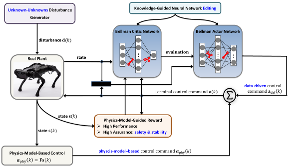
Figure 1: Physics-model-regulated deep reinforcement learning in training.

Generally, a safe stable system shall have a property that starts from a safe region and will eventually converge to the goal state while staying inside the safe region. To pertain to this property, model-based approaches focus on constructing a safety set, and the DRL agent is only allowed to act in this constrained space [7, 44, 37, 3, 38, 15]. In this direction, the control Lyapunov function (CLF) is typically used to constraint the state space with the objective that all actions will lead the system to decent on defined CLF, i.e., towards being stable [37, 3]. The difficulty that arises from those approaches is finding a CLF. Given the desired safety specification, one can also leverage control barrier function [7, 38] and reachability analysis [15] to certify the control command to satisfy the safety requirement. The approaches [7, 38, 15] are mainly designed to ensure the safety of the system, where how to guarantee stability remains an open problem. Moreover, the model-based approaches are generally limited to modeling errors and rely on a more accurate dynamics model to expand the safe region [7, 3]. Learning-based approaches, on the other hand, aim to embed the knowledge of safety and stability during training, such that the agent is guided to learn to stabilize the system [5, 50]. For example, Chang and Gao in [5] proposed to learn a Lyapunov function from sampled data and use it as an additional critic network to regulate the control policy, optimization toward the decrease of the Lyapunov critic values. The challenge moving forward is how to design DRL to exhibit mathematically-provable stability. Recently, the seminal work [50] discovered that if the reward of DRL is CLF-like, the systems controlled by a well-trained DRL agent can be mathematically-provable stable. Building on the work, the open problems moving forward are

• What is the formal guidance for constructing such CLF-like rewards for DRL?

• How to design DRL to concurrently guarantee safety and stability?

Another safety concern stems from the data-driven DNN adopted by DRL for the powerful function approximation and representation learning of action-value function, action policy, and environment states [34, 40], to name a few. However, it was recently discovered that purely data-driven DNN applied to physical systems can infer relations violating physics laws and sometimes lead to catastrophic consequences (e.g., data-driven blackout owning to violation of physical limits [53]). This thus induces the safety concern to DRL. The critical flaw in purely data-driven DNN motivates the emerging research on physics-enhanced DNN. Current frameworks include physics-informed NN [48, 51, 21, 20, 49, 31, 6, 45, 52, 23, 47, 11, 9, 14, 17], physics-guided NN architectures [36, 33, 35, 18, 46, 28] and physics-inspired neural operators [32, 29]. The physics-informed networks and physics-guided architectures use compact partial differential equations (PDEs) for formulating training loss functions and/or architectural components. Physics-inspired neural operators, such as the Koopman neural operator [32] and the Fourier neural operator [29], on the other hand, map nonlinear functions into alternative domains via fully-connected NNs, where it is easier to train their parameters from observational data and reason about convergence. These frameworks improve consistency degree with prior analytical knowledge, but remain problematic in several respects, especially when applied to DRL. For example, the critic network of DRL is to learn or estimate the expected future reward, also known as the Q-value. While the Q-value involves unknown future rewards, its compact or precise governing equation is thus not available at hand for physics-informed networks and physics-guided architectures. Additionally, the fully-connected NNs can introduce spurious correlations that deviate from strict compliance with available physical knowledge, which is still a safety concern of physics-inspired neural operators.

Fianlly, the unknown unknowns pose another formidable safety challenge, as they refer to outcomes, events, circumstances, or consequences that are not known in advance and cannot be predicted. Differentiating from known unknowns that have adequate historical data, the unknown unknowns have almost zero historical data at hand. The unknown unknowns thus can induce unseen real-time samples that are very distinct from training datasets. The control commands from DRL models (trained with stationary distribution) could result in unintended behavior or malfunction for systems operating in unknown-unknown environments, such as the unforeseen 2022 Central Illinois Freezing (resulted in a large number of car crashes).

To address the aforementioned safety concerns, we propose the Phy-DRL: a novel physics-model-regulated deep reinforcement learning framework for enhancing safety assurances. The Phy-DRL framework is shown in Figure 1, which has two novel components:

• Mathematical Foundations of Unknown-Unknowns Disturbances, which provide a guidance for generating unknown-unknowns disturbances for Phy-DRL’s proactive unknown-unknowns training. The training aims to empower a trained Phy-DRL to tolerate real-time unknown-unknowns disturbances.

• Conjunctive Residual Control and Safety-Embedded Reward, because of which, the Phy-DRL has mathematically-provable safety and stability guarantees.

• Physics-Model-Based Neural Network Editing, which includes link editing and activation editing, for embedding the available knowledge into inside of critic and actor networks to guarantee strict compliance with available physical knowledge.

2 Preliminaries

2.1 Notation and Terminology

For convenience, Table 1 summarizes the notations used throughout the paper. Note, the Real Plant, the States and the Control Commands presented in this proposal, respectively, correspond to the Environment, the Observations and the Actions in RL community.

Table 1: Table of Notation

$\mathbb{R}^{n}$: set of n-dimensional real vectors	$\mathbb{N}$: set of natural numbers
$\text{len}(\mathbf{s})$: length of vector $\mathbf{s}$	$[\mathbf{x}]_{i}$: $i$-th entry of vector $\mathbf{x}$
$[\mathbf{W}]_{i,:}$:  $i$-th row of matrix $\mathbf{W}$	$[\mathbf{W}]_{i,j}$:  element at row $i$ and column $j$ of matrix $\mathbf{W}$
$\mathbf{P}\succ 0$:  matrix $\mathbf{P}$ is positive definite	$\top$: matrix or vector transposition
$\mathbf{I}_{n}$:  $n\times n$-dimensional identity matrix	$\mathbf{1}_{n}$:  $n$-dimensional vector of all ones

2.2 Dynamics Model of Real Plant

Without loss of generality, the dynamics of a real plant is described by

$$\mathbf{s}(k+1)={\mathbf{A}}\cdot\mathbf{s}(k)+{\mathbf{B}}\cdot\mathbf{a}(k)+\mathbf{f}(\mathbf{s}(k),\mathbf{a}(k),\mathbf{d}(k)),~{}~{}~{}~{}k\in\mathbb{N}$$ (1)

where $\mathbf{f}(\mathbf{s}(k),\mathbf{a}(k),\mathbf{d}(k))\in\mathbb{R}^{n}$ is the unknown model mismatch, $\mathbf{d}(k)\in\mathbb{R}^{o}$ is the disturbance, ${\mathbf{A}}\in\mathbb{R}^{n\times n}$ and ${\mathbf{B}}\in\mathbb{R}^{n\times m}$ denote known system matrix and control structure matrix, respectively, $\mathbf{s}(k)\in\mathbb{R}^{n}$ is the real-time system state, $\mathbf{a}(k)\in\mathbb{R}^{m}$ is the vector of real-time control commands. Summarily, the available knowledge pertaining to real plant (1) is represented by $\left\{{\mathbf{A},~{}\mathbf{B}}\right\}$.

2.3 Safety Set

The considered safety problem stems from regulations or safety constraints on system states, which motives the following safety set ${\mathbb{X}}$.

Safe State Set: $${\mathbb{X}}\triangleq\left\{{\left.{\mathbf{s}\in{\mathbb{R}^{n}}}\right|\underline{\mathbf{v}}\leq{\mathbf{D}}\cdot\mathbf{s}-\mathbf{v}\leq\overline{\mathbf{v}}}\right\}.$$ (2)

where $\mathbf{D}$, $\mathbf{v}$, $\overline{\mathbf{v}}$ and $\underline{\mathbf{v}}$ are given in advance.

Remark 2.1 (Safety Example).

The condition for formulating the safety set (2) can cover a significant number of safety problems that are associated with operation regulations and/or safety constraints. Considering autonomous vehicles driving in a school zone in Winter as one example, according to traffic regulations, the vehicle speed shall be around 15 mph. To prevent slipping and sliding for safe driving on icy roads, the vehicle slip shall not be larger than 4 mph. Given the information on regulation and safety constraints, we can let

$$\mathbf{s}=\left[\!\begin{array}[]{l}v\\ w\end{array}\!\right]\!,~{}~{}~{}\mathbf{D}=\left[\!{\begin{array}[]{*{20}{c}}1\!&\!0\\ 1\!&\!{-r}\end{array}}\!\right],~{}~{}~{}\mathbf{v}=\left[\!\begin{array}[]{l}15\\ 0\end{array}\!\right]\!,~{}~{}~{}\overline{\mathbf{v}}=\left[\!\begin{array}[]{l}2\\ 4\end{array}\!\right]\!,~{}~{}~{}\underline{\mathbf{v}}=\left[\!\begin{array}[]{l}-2\\ -4\end{array}\!\right],$$ (13)

such that the condition in (2) can equivalently transform to

$$-2\leq v-15\leq 2,~{}~{}~{}~{}~{}~{}~{}~{}~{}~{}~{}~{}~{}-4\leq v-r\cdot w\leq 4,$$

where $v$, $w$, and $r$ denote the vehicle’s longitudinal velocity, angular velocity and wheel radius, respectively. The first inequality means the allowable maximum difference with traffic-regulated velocity (i.e., 15 mph) is 2 mph. While the second inequality means the vehicle slip (defined as $v-r\cdot w$) is constrained to be no larger than 4 mph.

Based on the safety set, we present the definitions pertaining to safety and stability.

Definition 2.2.

Consider the safety set $\mathbb{X}$ (2). The real plant (1) is said to be safety guaranteed, if $\mathbf{s}(1)\in{\mathbb{X}}$, then $\mathbf{s}(k)\in{\mathbb{X}}$ for any $k>1\in\mathbb{N}$.

Definition 2.3.

The real plant (1) is said to be stability guaranteed, if given any $\mathbf{s}(1)\in\mathbb{R}^{n}$, then $\mathop{\lim}\limits_{k\to\infty}\mathbf{s}(k)=\mathbf{0}$.

2.4 Mathematical Foundations of Unknown-Unknowns Disturbances

The proactive unknown-unknowns training aim to enable a trained Phy-DRL to tolerate unknown-unknowns disturbances. A prerequisite to developing such training mechanism is to have the formal mathematical foundations of unknown-unknowns disturbance, according to which the unknown-unknowns disturbances can automatically and proactively generated for Phy-DRL training. To do so, we propose a variant of Beta distribution to mathematically define the unknown-unknowns disturbances:

Definition 2.4.

The disturbance $\mathbf{d}(k)$ in the dynamics model (1) is said to be bounded unknown-unknowns, if (i) $\mathbf{d}(k)\sim\textit{Beta}(\alpha(k),\beta(k),c,a)$, and (ii) $\alpha(k)$ and $\beta(k)$ are random parameters. In other words, the disturbance $\mathbf{d}(k)\in[a,c]$ and its probability density function (pdf) is

$$f\left({\mathbf{d}(k);~{}\alpha(k),~{}\beta(k),~{}a,~{}c}\right)=\frac{{{{\left({\mathbf{d}(k)-a}\right)}^{\alpha-1}}{{\left({c-\mathbf{d}(k)}\right)}^{\alpha(k)-1}}\Gamma\left({\alpha(k)+\beta(k)}\right)}}{{{{\left({c-a}\right)}^{\alpha(k)+\beta(k)-1}}\Gamma\left(\alpha(k)\right)\Gamma\left(\beta(k)\right)}},$$ (14)

where $\Gamma\left(\alpha(k)\right)=\int_{0}^{\infty}{{t^{\alpha(k)-1}}{e^{-t}}dt},~{}{\mathop{\rm Re}\nolimits}\left(\alpha(k)\right)>0$, $\alpha(k)$ and $\beta(k)$ are randomly given at every $k$.

Remark 2.5 (Motivations).

The motivation behind the bounds (i.e., $a$ and $c$) on the unknown-unknowns disturbances is that in general, no human solutions exist for manipulating unbounded unknown-unknowns disturbances, such as earthquakes and volcanic eruptions. While the motivation behind the random $\alpha(k)$ and $\beta(k)$ is that the unknown unknowns usually are beyond the scope of nature and science, which lead to unavailable model for scientific discoveries and understating. Besides, the $\alpha(k)$ and $\beta(k)$ directly control the mean and variance of $\mathbf{d}(k)$ and its pdf formulas. If the $\alpha(k)$ and $\beta(k)$ are random, the distribution of $\mathbf{d}(k)$ can be uniform distribution, exponential distribution, truncated Gaussian distribution, or mixed of them, or many others, but is unknown! Therefore, the random $\alpha(k)$ and $\beta(k)$ can well capture the “unavailable model" and “unforeseen" traits of unknown unknowns.

2.5 Problem Formulation

The aim of this paper is to design DRL to particularly enhance its robustness and safety assurance for safety-critical autonomous systems. The investigated problems are formally stated below.

Problem 2.6.

How to leverage the available knowledge pertaining to real plant (1), i.e., $\left\{{\mathbf{A},~{}\mathbf{B}}\right\}$, to design DRL to achieve safety and stability guarantees?

Problem 2.7.

How to develop end-to-end critic and actor networks that can strictly comply with available physical knowledge pertaining to the action-value function, reward, Bellman equation and control policy?

The proposed solution to the Problems 2.6 and 2.7 is the physics-model-regulated deep reinforcement learning (Phy-DRL), whose framework is shown in Figure 1. The Phy-DRL designs are detailed in following sections.

3 Phy-DRL: Residual Control and Safety-Embedded Reward

3.1 Residual Control

As shown in Figure 1, the terminal control command $\mathbf{a}(k)$ from Phy-DRL is given in residual form:

$$\mathbf{a}(k)=\mathbf{a}_{\text{drl}}(k)+\mathbf{a}_{\text{phy}}(k),$$ (15)

where the $\mathbf{a}_{\text{drl}}(k)$ denotes date-driven control command from DRL, while the $\mathbf{a}_{\text{phy}}(k)$ is model-based control command, computed according to according to

$$\mathbf{a}_{\text{phy}}(k)=\mathbf{F}\cdot\mathbf{s}(k).$$ (16)

We note the $\mathbf{F}$ in (16) is designed based on the physics-model knowledge $\left\{{\mathbf{A},\mathbf{B}}\right\}$. The developed Phy-DRL is based on the deep deterministic policy gradient algorithm [30], which learns a deterministic control policy $\pi(\mathbf{s}(k))=\mathbf{a}_{\text{drl}}(k)$ that maximizes the expected return from the initial state distribution:

$${\mathcal{Q}^{\pi}}({\mathbf{s}(k),\mathbf{a}_{\text{drl}}(k)})={\mathbf{E}_{\mathbf{s}(k)\sim\mathbb{S}}}\left[{\sum\limits_{t=k}^{N}{{\gamma^{t-k}}\cdot\mathcal{R}\left(\mathbf{s}(k),\mathbf{a}_{\text{phy}}(k)\right)}}\right],$$ (17)

where $\mathbb{S}$ represents the state space, $\mathcal{R}(\cdot)$ maps a state-action-next-state triple to a real-valued reward, $\gamma\in[0,1]$ is the discount factor, controlling the relative importance of immediate and future rewards. The expected return (17) and control policy $\pi$ are parameterized by the critic and actor networks, respectively.

3.2 Safety-Embedded Reward

The current safety formula (2) is not ready for constructing the safety-embedded reward yet. To pave the way, we introduce a safety envelope:

$${\Omega}\triangleq\left\{{\left.{\mathbf{s}\in{\mathbb{R}^{n}}}\right|{\mathbf{s}^{\top}}\cdot{\mathbf{P}}\cdot\mathbf{s}\leq 1,~{}{\mathbf{P}}\succ 0}\right\}.$$ (18)

The following lemma builds a connection between the sets (18) and (2), whose formal proof appears in Appendix B of Supplementary Material.

Lemma 3.1.

Consider the sets defined in Equations (2) and (18). We have

$${\Omega}\subseteq\mathbb{X},~{}~{}~{}\text{if}~{}~{}\left[\overline{\mathbf{D}}\right]_{i,:}\cdot{\mathbf{P}^{-1}}\cdot\left[\overline{\mathbf{D}}^{\top}\right]_{:,i}\leq 1$$

$$\hskip 83.93553pt\text{and}~{}\left[\underline{\mathbf{D}}\right]_{i,:}\cdot{\mathbf{P}^{-1}}\cdot\left[\underline{\mathbf{D}}^{\top}\right]_{:,i}=\begin{cases}\geq 1,\!\!&\text{if}~{}~{}[{\mathbf{d}}]_{i}=1\\ \leq 1,\!\!&\text{if}~{}~{}[{\mathbf{d}}]_{i}=-1\end{cases}\!,~{}~{}~{}i\in\{1,2,\ldots,h\}$$ (19)

where ${\mathbf{d}}$ is defined in (38) in Appendix A of Supplementary Material, $\overline{\mathbf{D}}=\frac{{\mathbf{D}}}{\overline{\Lambda}}$ and $\underline{\mathbf{D}}=\frac{{\mathbf{D}}}{\underline{\Lambda}}$, with $\overline{\Lambda}$, and $\underline{\Lambda}$ given in (39) and (40), respectively, in Appendix A of Supplementary Material.

Given the model knowledge $\left\{{\mathbf{A},~{}\mathbf{B}}\right\}$, the safety envelope (18) and the model-based control (16), the proposed safety-embedded reward is

$$\mathcal{R}({\mathbf{s}(k),\mathbf{a}_{\text{drl}}}(k))=\underbrace{\mathbf{s}^{\top}(k)\cdot{{\overline{\mathbf{A}}^{\top}}\cdot\mathbf{P}\cdot\overline{\mathbf{A}}}\cdot\mathbf{s}(k)-{\mathbf{s}^{\top}(k+1)}\cdot\mathbf{P}\cdot\mathbf{s}(k+1)}_{\triangleq~{}r(\mathbf{s}(k),~{}\mathbf{a}(k))}~{}~{}+~{}w(\mathbf{s}(k),\mathbf{a}(k)),$$ (20)

where the sub-reward $r(\mathbf{s}(k),\mathbf{a}(k))$ is safety-embedded, while the sub-reward $w(\mathbf{s}(k),\mathbf{a}(k))$ aims at high performance operation, and we define:

$$\overline{\mathbf{A}}\buildrel\Delta\over{=}\mathbf{A}+{\mathbf{B}}\cdot{\mathbf{F}}.$$ (21)

In current reward formula, the matrices ${\mathbf{F}}$ and ${\mathbf{P}}$ are unknown. The problem moving forward is to design ${\mathbf{F}}$ and ${\mathbf{P}}$ for Phy-DRL towards safety and stability guarantees, which is conducted in the next subsection.

3.3 Mathematically-Provable Safety and Stability Guarantees

The following theorem presents the conditions on ${\mathbf{F}}$ and ${\mathbf{P}}$, for Phy-DRL towards safety, as well as stability, guarantees, whose proof is given in Appendix C of Supplementary Material.

Theorem 3.2.

Consider the system (1) under the residual control, consisting of (15) and (16), of Phy-DRL, the safety-embedded reward (20), and the sets ${\mathbb{X}}$ and ${\Omega}$ defined in (2) and (18), respectively. If matrices $\mathbf{F}$ and $\mathbf{P}$ involved therein are computed according to

$$\mathbf{F}=\mathbf{R}\cdot\mathbf{Q}^{-1},~{}~{}~{}~{}\mathbf{P}=\mathbf{Q}^{-1},$$ (22)

where $\mathbf{R}$ and $\mathbf{Q}^{-1}$ satisfies the inequalities (19) and

$$\left[{\begin{array}[]{*{20}{c}}\alpha\cdot\mathbf{Q}&\mathbf{Q}\cdot\mathbf{A}^{\top}+\mathbf{R}^{\top}\cdot\mathbf{B}^{\top}\\ \mathbf{A}\cdot\mathbf{Q}+\mathbf{B}\cdot\mathbf{R}&\mathbf{Q}\end{array}}\right] \succ 0,$$ (25)

for given $0<\alpha<1$, then,

1. If the sub-reward $r(\mathbf{s}(k),\mathbf{a}(k))$ in (20) satisfies $r(\mathbf{s}(k),\mathbf{a}(k))\geq\alpha-1$, the safety of real plant (1) under control of Phy-DRL is guaranteed, i.e., $\mathbf{s}(k)\in{\Omega}\subseteq\mathbb{X}$, $\forall k\in\mathbb{N}$, if $\mathbf{s}(1)\in{\Omega}$.

2. If the sub-reward $r(\mathbf{s}(k),\mathbf{a}(k))$ in (20) satisfies $r(\mathbf{s}(k),\mathbf{a}(k))>(\alpha-1)\cdot{\mathbf{s}^{\top}(k)}\cdot{\mathbf{P}}\cdot\mathbf{s}(k)$, the safety and stability of real plant (1) under control of Phy-DRL are guaranteed.

Remark 3.3 (Model-Based Design).

Solving the matrices from inequalities (19) and (25) while maximizing the safety envelope (18) is a typical analytic centering problem [43], which can be solved via the CVXPY toolbox [13] in Python. One such example is given in Appendix G.2 of Supplementary Material.

Remark 3.4 (Safety and Stability Evaluation).

The results presented in Theorem 3.2 are ready for evaluating the safety and stability of a Phy-DRL for stopping or continuing the training, since the terms $r(\mathbf{s}(k),\mathbf{a}(k))$, $\alpha$ and ${\mathbf{s}^{\top}(k)}\cdot{\mathbf{P}}\cdot\mathbf{s}(k)$ included in conditions are defined by system operator in advanced, and their (real-time) values can be observed during Phy-DRL training.

4 Phy-DRL: Knowledge-Enhanced Critic and Actor Networks

This section focuses on the solution to Problem 2.7. The Phy-DRL is built on the deep deterministic policy gradient (DDPG) algorithm [30], which consists of critic and actor networks.

4.1 Critic and Actor Networks

The critic network of Phy-DRL uses neural networks to learn the action-value function. Specifically, the critical network is parameterized by ${\theta^{Q}}$, which aims to minimize the loss:

$$\mathcal{L}\left({{\theta^{\mathcal{Q}}}}\right)={\mathbf{E}_{{\mathbf{s}(k){\sim\mathbb{S}}}}}\left[\left(\mathcal{Q}({\left.{{\mathbf{s}(k)},{\mathbf{a}_{\text{drl}}(k)}}\right|{\theta^{\mathcal{Q}}}})-{\mathbf{y}(k)}\right)^{2}\right],$$ (26)

where

$${\mathbf{y}(k)}=\mathcal{R}\left({{\mathbf{s}(k)},{\mathbf{a}_{\text{drl}}(k)}}\right)+\gamma\cdot\mathcal{Q}\left({\left.{{\mathbf{s}(k+1)},{\mathbf{a}_{\text{drl}}(k+1)}}\right|{\theta^{\mathcal{Q}}}}\right).$$ (27)

The actor network of Phy-DRL parameterized by ${\eta^{\pi}}$, is to learn a deterministic control policy. Summarily, the objective of DRL training is to find the optimal control policy $\pi_{\eta}$ that can maximize the expected return

$$\mathcal{J}\left(\pi_{\eta}\right)={\mathbf{E}_{\mathbf{s}_{k}\sim\mathbb{S}}}\left[{\sum\limits_{t=k}^{N}{{\gamma^{t-k}}\cdot\mathcal{R}\left(\mathbf{s}(k),\pi_{\eta}(\mathbf{s}(k))\right)}}\right].$$

According to the work of DPG [41], with the consideration of (17), the actor network is updated according to the control policy gradient:

$$\frac{{\partial\mathcal{J}\left({{\pi_{\eta}}}\right)}}{{\partial\eta}}={\mathbf{E}_{{\mathbf{s}_{k}}\sim\mathbb{S}}}\left[{\frac{{\partial\mathcal{Q}\left(\mathbf{s}(k),\pi_{\eta}(\mathbf{s}(k))\right)}}{{\partial{\pi_{\eta}}\left({{\mathbf{s}_{k}}}\right)}}\cdot\frac{{\partial{\pi_{\eta}}\left({{\mathbf{s}_{k}}}\right)}}{{\partial\eta}}}\right].$$ (28)

The reward is defined by the system operator in advance. Moreover, the (26)–(28) indicate that updates of critic and actor networks rely on the principle of Bellman equation. Furthermore, the Bellman equation, in turn, is a direct function of reward. Therefore, there can exist plentiful physical knowledge at hand that the critic and actor networks shall strictly comply with. For example, if in the reward formula (20), the $w(\mathbf{s}(k),\mathbf{a}(k))=0$, according to the Bellman equation, the available physical knowledge is that the action-value function ${\mathcal{Q}^{\pi}}({\mathbf{s}(k),\mathbf{a}_{\text{drl}}(k)})$ does not include the odd-order monomials $\mathbf{s}(k)$ and $\mathbf{u}_{\text{drl}}(k)$. Moreover, the action-value function involves future rewards. Therefore, a compact and precise governing equation of action-value function is not available for regulating the training loss function, which thus hinders the applications of current frameworks of physics-enhanced DNN here [48, 51, 21, 20, 49, 31, 6, 45, 52, 23, 47, 11, 9, 14, 17, 36, 33, 35, 18, 46, 28]. In summary, the challenge is only partial knowledge pertaining to the action-value function and/or control policy are available, but are hidden in the Bellman equation, the reward formula and the control policy gradient. The design of physical knowledge-enhanced critic and actor networks is to guarantee their strict compliance with the available partial knowledge. To formulate the problem, we describe the ground-truth models of action-value function and control policy as follows.

$$\mathcal{Q}\left(\mathbf{s}(k),\mathbf{a}_{\text{drl}}(k)\right) =\underbrace{\mathbf{A}_{\mathcal{Q}}}_{\text{weight matrix}}\cdot\underbrace{\mathfrak{m}(\mathbf{s}(k),\mathbf{a}_{\text{drl}}(k),{r}_{\mathcal{Q}})}_{\text{node-representation vector}}+\underbrace{\mathbf{p}(\mathbf{s}(k),\mathbf{a}_{\text{drl}}(k))}_{\text{model mismatch}}\in\mathbb{R},$$ (29)

$$\pi\left(\mathbf{s}(k)\right) =\underbrace{\mathbf{A}_{\pi}}_{\text{weight matrix}}\cdot\underbrace{{\mathfrak{m}}(\mathbf{s}(k),{r}_{\pi})}_{\text{node-representation vector}}+\underbrace{{\mathbf{p}}(\mathbf{s}(k))}_{\text{model mismatch}}\in\mathbb{R}^{\text{len}(\pi\left(\mathbf{s}(k)\right))},$$ (30)

based on this, we define the following knowledge set that includes the available physical knowledge of critic and actor networks.

$$\!\!\!\!\!\mathbb{K}_{\mathcal{Q}} \!\triangleq\!\left\{{{\left[\mathbf{A}_{\mathcal{Q}}\right]}_{i}\left|{\frac{{\partial\mathbf{p}({{\mathbf{s}(k)},\mathbf{a}_{\text{drl}}(k)})}}{{\partial{{\left[\mathfrak{m}({\mathbf{s}(k)},{\mathbf{a}_{\text{drl}}(k),{r}_{\mathcal{Q}})}\right]}_{i}}}}\equiv 0,~{}~{}i\in\left\{{1,~{}2,~{}\ldots,~{}\text{len}({\mathfrak{m}({{\mathbf{s}_{k}},{\mathbf{a}_{\text{drl}}(k)}})},{r}_{\mathcal{Q}})}\right\}}\right.}\right\}\!,$$ (31)

$$\!\!\!\!\!\mathbb{K}_{\pi} \!\triangleq\!\left\{\!\!{\left.{{{\left[\mathbf{A}_{\pi}\right]}_{i,j}}}\right|\frac{{\partial[{\mathbf{p}}({{\mathbf{s}(k)}})]_{i}}}{{\partial{{\left[{{\widehat{\mathfrak{m}}}({{\mathbf{s}(k),{r}_{\mathcal{\pi}}}})}\right]}_{j}}}}\!\equiv\!0,~{}i\!\in\!\left\{{1,\ldots,\text{len}(\pi(\mathbf{s}(k)))}\right\}\!,\!~{}j\!\in\!\left\{{1,\ldots,\text{len}({\widehat{\mathfrak{m}}({{\mathbf{s}(k),{r}_{\mathcal{\pi}}}})})}\right\}}\!\!\right\}\!.$$ (32)

We next present the design of physical knowledge-enhanced NN, which aims to embed all the knowledge in sets (31) and (32) to the critic and actor networks, respectively.

4.2 Knowledge-Enhanced DNN Architecture

As shown in Figure 2, the knowledge-enhanced DNN has two innovations in neural architecture: (i) Physics-Model-Guided Neural Network (NN) Editing and (ii) NN Input Augmentation. We note from Figure 2 (b) that the NN input augmentation is incorporated into NN inside, creating the physics-compatible neural network (PhyN).

The NN input augmentation is formally described by Algorithm 1 in Appendix D of Supplementary Material. The augmentation component aims at two targeted capabilities for critic and actor networks:

• Non-linear Physics Representation: The generated high-order monomials directly capture the core hard-to-learn nonlinearities of physical quantities such as kinetic energy ($\triangleq\frac{1}{2}m{v^{2}}$), potential energy ($\triangleq\frac{1}{2}k{x^{2}}$), electrical power ($\triangleq V\cdot I$) and aerodynamic drag force ($\triangleq\frac{1}{2}\rho{v^{2}}{C_{D}}A$), that drive the state dynamics of physical systems.

• Controllable Model Accuracy: The ultimate purpose of NN input augmentation is to approximate the ground-truth model via polynomial function. Then according to the Stone–Weierstrass theorem [42], the DNN can have controllable model accuracy by controlling the augmentation orders.

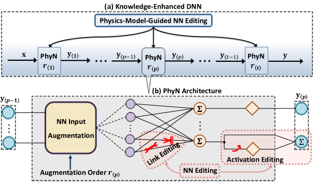
Figure 2: Knowledge-Enhanced DNN architecture.

Showing in Figure 2 (b), the NN editing includes link editing and activation editing for embedding the prior well-validated physical knowledge into NN inside, such that the critic and actor networks can strictly comply with the available physical knowledge or laws while avoiding spurious correlations. The procedure of NN editing described by Algorithm 2 and its detailed explanations are presented in Appendix E of Supplementary Material. Thanks to the NN editing, the input/output of critic and actor networks can strictly comply with the available physical knowledge, which is formally presented in the following theorem, whose proof appears in Appendix F of Supplementary Material.

Theorem 4.1.

Give knowledge sets $\mathbb{K}_{\mathcal{Q}}$ (31) and $\mathbb{K}_{\pi}$ (32), consider the critic and actor networks built on knowledge-enhanced DNN (described in Figure 2) with NN editing via Algorithm 2 in Appendix E of Supplementary Material. The inputs/outputs of critic and actor networks strictly comply with the available knowledge pertaining to the models (31) and (32) of ground truth. In other words,

• For input and output of critic network, i.e., $\mathbf{x}=\left[\mathbf{s}(k);\mathbf{a}_{\text{drl}}(k)\right]$ and $\mathbf{y}=\widehat{\mathcal{Q}}\left(\mathbf{s}(k),\mathbf{a}_{\text{drl}}(k)\right)$, if $[\mathbf{A}_{\mathcal{Q}}]_{i}\in\mathbb{K}_{\mathcal{Q}}$, then $\frac{{\partial{\widehat{\mathbf{y}}}}}{\partial[\mathfrak{m}(\mathbf{s}(k),\mathbf{a}_{\text{drl}}(k),{r}_{\mathcal{Q}})]_{i}}\equiv\frac{{\partial{\widehat{\mathcal{Q}}\left(\mathbf{s}(k),\mathbf{a}_{\text{drl}}(k)\right)}}}{\partial[\mathfrak{m}(\mathbf{s}(k),\mathbf{a}_{\text{drl}}(k),{r}_{\mathcal{Q}})]_{i}}\equiv[\mathbf{A}_{\mathcal{Q}}]_{i}$ always hold.

• For input and output of actor network, i.e., $\mathbf{x}=\mathbf{s}(k)$ and $\mathbf{y}=\widehat{\pi}\left(\mathbf{s}(k)\right)$, if $[\mathbf{A}_{\pi}]_{i,j}\in\mathbb{K}_{\pi}$, then $\frac{{\partial{[{\mathbf{y}}]_{i}}}}{\partial[\widehat{\mathfrak{m}}(\mathbf{s}(k),{r}_{\pi})]_{j}}\equiv\frac{{\partial{[\widehat{\pi}\left(\mathbf{s}(k)\right)]_{i}}}}{\partial[\widehat{\mathfrak{m}}(\mathbf{s}(k),{r}_{\pi})]_{j}}\equiv[\mathbf{A}_{\pi}]_{i,j}$ always hold.

5 Experiments

The demonstrations are performed on a car-pole system and a quadruped robot.

5.1 Car-Pole System

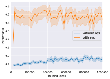
(a)

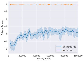
(b)

Figure 3: Training Comparisons.

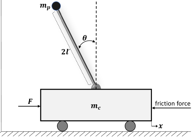
Figure 9: Mechanical analog of inverted pendulums.

We here take the cart-pole simulator provided in Open-AI Gym [4] and adapt it to a more realistic system with friction and continuous action space. The inverted pendulum system, whose mechanical analog is shown in Figure 9 in Appendix G of Supplementary Material, is characterized by the angle $\theta$ of the pendulum from vertical, the angular velocity $\omega\buildrel\Delta\over{=}\dot{\theta}$, the position $x$ and velocity $v\buildrel\Delta\over{=}\dot{x}$ of the cart. The mission of a trained Phy-DRL is to stabilize the pendulum at the equilibrium $\mathbf{s}^{*}=[x^{*},v^{*},\theta^{*},\omega^{*}]^{\top}=[0,0,0,0]^{\top}$, while constraining pendulum angle and car position of system and model-based control commands to the regions:

$$-0.9\leq x\leq 0.9,~{}~{}~{}-0.8\leq\theta<0.8,~{}~{}~{}-16\leq\mathbf{a}_{\text{phy}}<16.$$ (33)

To convincingly demonstrate the robustness of Phy-DRL, the model-based design ignore road friction force, such that sole model-based control commands cannot achieve the safe control mission, which can be demonstrated by the trajectories shown in Figure 10 in Appendix G.3 of Supplementary Material. The $\mathbf{F}$, $\mathbf{P}$ and $\overline{\mathbf{A}}$ of model-based control (16) and safety-embedded reward (20), with $w(\mathbf{s}(k),\mathbf{a}_{\text{drl}}(k))=-\mathbf{a}_{\text{drl}}^{2}(k)$, are given in (125), (123) and (130) in Appendix G.2 of Supplementary Material. Moreover, the Appendices G.1 and G.2 include details of model-based design. Before moving forward, we introduce the following samples for presenting experimental comparisons.

Safe-Internal-Envelope (IE) Sample $$\triangleq\widetilde{\mathbf{s}} \text{if}~{}\mathbf{s}(1)=\widetilde{\mathbf{s}}\in{\Omega},~{}\text{then}~{}\mathbf{s}(k)\in{\Omega}~{}\text{for any}~{}k\in\mathbb{N}.$$: (34)

Safe-External-Envelope (EE) Sample $$\triangleq\widetilde{\mathbf{s}} \text{if}~{}\mathbf{s}(1)=\widetilde{\mathbf{s}}\notin\Omega,~{}\text{then}~{}\mathbf{s}(k)\in\mathbb{X}~{}\text{for any}~{}k\in\mathbb{N}.$$: (35)

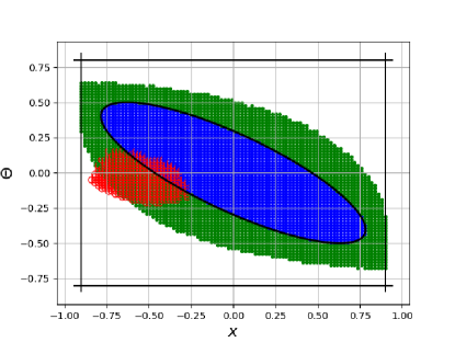
Figure 4: Areas of samples: blue dot: IE of Phy-DRL, green dot: EE of Phy-DRL, red dot: IE of Phy-DRL with CLF, red circle: EE of DRL with CLF, blue area: safety envelope.

In the experiments, we compare Phy-DRL with purely data-driven DRL from the perspectives of training and testing. For training, we consider metrics: i) the average reward over episode and ii) safety and stability performance, i.e., $p(k)=e^{-d(k)}$ with $d(k)$ measuring the Euclidean distance between the pole tip at time $k$ and the equilibrium point. For the testing, we will compare the safety areas of trained models, which are defined by the area of safe samples in (34) and (35). All of the comparison models are trained for $10^{6}$ steps. This experiment mainly demonstrates the effectiveness of residual control and safety-embedded reward. So, all of the experimental models have the same network configurations, except for their rewards and terminal control commands. The network configurations are presented in Appendix G.4 of Supplementary Material.

The influence of residual control on training is presented in Figure 3, where both Phy-DRL and purely data-driven use the same reward, but the purely data-driven one does not have the model-based control commands. Figure 3 demonstrates that incorporating model-based design into DRL can significantly enlarge episode reward, safety and stability performance and speed up training.

Recently, the seminal work [50] discovered that if the reward of DRL is a control Lyapunov function (CLF), a well-trained DRL can exhibit a mathematically-provable stability guarantee. The CLF-like reward (we here let $\mathcal{R}(\cdot)=\mathbf{s}^{\top}(k)\cdot\mathbf{P}\cdot\mathbf{s}(k)-{\mathbf{s}^{\top}(k+1)}\cdot\mathbf{P}\cdot\mathbf{s}(k+1)+w(\mathbf{s}(k),\mathbf{a}(k))$) is very similar to our safety-embedded one (20). It is the minor difference, in conjunction with residual control design, that empowers the Phy-DRL with the trait of mathematically-provable safety and stability guarantees. This can be observed from areas of safe samples in Figure 4 that i) the Phy-DRL successfully renders the safety envelope guided by physic-model invariant, demonstrating the first statement of Theorem 3.2, ii) purely data-driven DRL with CLF reward can discover a safe area that Phy-DRL does not preserve (i.e., no overlapped red area), but its overall safe area is much smaller than Phy-DRL (given the same training steps and configurations of critic and actor networks). More comprehensive comparisons are presented in Appendix G.5 of Supplementary Material.

5.2 Quadruped Robot

Important Note: Due to page limit, the experimental results pertaining to NN editing are presented in the Appendix H.3 of Supplementary Material.

The mission of Phy-DRL for the quadruped Robot is to regulate the CoM (center of mass) velocity alone x-axis to 1 m/s at the CoM height 0.24 m, under the safety constraints:

$$\left|{\text{CoM Height}-0.24~{}\text{m}}\right|\leq 0.1~{}\text{m},~{}~{}\left|{\text{CoM x-velocity}-1\text{m/s}}\right|\leq 1\text{m/s}.$$ (36)

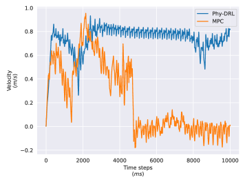
(a)

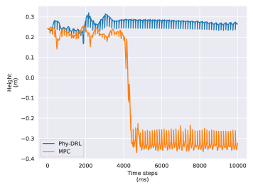
(b)

Figure 5: Trajectories of Robot running on the low-friction ground.

The model-based designs of residual control and safety-embedded reward are presented in Appendix H.1 of Supplementary Material. For the comparisons in this section, we consider the model predictive control (MPC) approach [10]. The comparisons with purely data-driven DRL are presented in Appendix H.2 of Supplementary Material. The trajectories in Figure 5 show that the robot under the control of Phy-DRL successfully achieves its safe mission on the low-friction (friction coefficient: $\mu=0.6$), while the sole MPC fails to work (robot dropped, indicated by Figure 5 (b)).

6 Conclusion and Discussion

This paper proposes the Phy-DRL: a physics-model-regulated deep reinforcement learning framework for safety-critical autonomous systems. The Phy-DRL is able to 1) have mathematically-provable safety and stability guarantees, and 2) strictly comply with physical knowledge. The effectiveness of the Phy-DRL has been validated by a cart-pole system and a quadruped robot. The experimental results demonstrate that compared with purely data-driven DRL, Phy-DRL features remarkably fewer learning parameters, accelerated training, and enlarged reward, while offering enhanced model robustness and safety assurance. Moving forward, we will investigate the influence of weights of data-driven control v.s. model-based control on system stability performance, safety guarantee, and convergence speed.

[sections] [sections]l1

Appendix A Auxiliary Lemmas

Lemma A.1 (Schur Complement [54]).

For any symmetric matrix $\mathbf{M}=\left[\!\!{\begin{array}[]{*{20}{c}}\mathbf{A}&\mathbf{B}\\ {{\mathbf{B}^{\top}}}&\mathbf{C}\end{array}}\!\!\right]$, then $\mathbf{M}\succ 0$ if and only if $\mathbf{C}\succ 0$ and $\mathbf{A}-\mathbf{B}\mathbf{C}^{-1}\mathbf{B}^{\top}\succ 0$.

Lemma A.2.

Corresponding to the set ${\mathbb{X}}$ (2), we define:

$${\widehat{\mathbb{X}}} \triangleq\left\{{\left.{\mathbf{s}\in{\mathbb{R}^{n}}}\right|-\mathbf{1}_{h}\leq{\mathbf{d}}\leq\underline{\mathbf{D}}\cdot\mathbf{s},~{}~{}~{}\text{and}~{}~{}\overline{\mathbf{D}}\cdot\mathbf{s}\leq\mathbf{1}_{h}}\right\},,$$ (37)

with

$$[{\mathbf{d}}]_{i} \triangleq\begin{cases}1,&\text{if}~{}\left[\underline{\mathbf{v}}+\mathbf{v}\right]_{i}>0\\ 1,&\text{if}~{}\left[\overline{\mathbf{v}}+\mathbf{v}\right]_{i}<0\\ -1,&\text{if}~{}\left[\overline{\mathbf{v}}+\mathbf{v}\right]_{i}\geq 0~{}\text{and}~{}\left[\underline{\mathbf{v}}+\mathbf{v}\right]_{i}\leq 0\end{cases},~{}~{}~{}~{}~{}i\in\{1,2,\ldots,h\}.$$ (38)

Then, the sets ${\mathbb{X}}=\widehat{{\mathbb{X}}}$, if and only if  $\overline{\mathbf{D}}=\frac{{\mathbf{D}}}{\overline{\Lambda}}$ and $\underline{\mathbf{D}}=\frac{{\mathbf{D}}}{\underline{\Lambda}}$, where for $i,j\in\{1,2,\ldots,h\}$,

$$[\overline{\Lambda}]_{i,j} \triangleq\begin{cases}0,&\text{if}~{}i\neq j\\ \left[\overline{\mathbf{v}}+\mathbf{v}\right]_{i},&\text{if}~{}\left[\underline{\mathbf{v}}+\mathbf{v}\right]_{i}>0\\ \left[\underline{\mathbf{v}}+\mathbf{v}\right]_{i},&\text{if}~{}\left[\overline{\mathbf{v}}+\mathbf{v}\right]_{i}<0\\ \left[\overline{\mathbf{v}}+\mathbf{v}\right]_{i},&\text{if}~{}\left[\overline{\mathbf{v}}+\mathbf{v}\right]_{i}\geq 0~{}\text{and}~{}\left[\underline{\mathbf{v}}+\mathbf{v}\right]_{i}\leq 0\end{cases},$$ (39)

$$[\underline{\Lambda}]_{i,j} \triangleq\begin{cases}0,&\text{if}~{}i\neq j\\ \left[\underline{\mathbf{v}}+\mathbf{v}\right]_{i},&\text{if}~{}\left[\underline{\mathbf{v}}+\mathbf{v}\right]_{i}>0\\ \left[\overline{\mathbf{v}}+\mathbf{v}\right]_{i},&\text{if}~{}\left[\overline{\mathbf{v}}+\mathbf{v}\right]_{i}<0\\ \left[-\underline{\mathbf{v}}-\mathbf{v}\right]_{i},&\text{if}~{}\left[\overline{\mathbf{v}}+\mathbf{v}\right]_{i}\geq 0~{}\text{and}~{}\left[\underline{\mathbf{v}}+\mathbf{v}\right]_{i}\leq 0\end{cases}.$$ (40)

Proof.

The condition of set (2) is equivalent to

$$\left[\underline{\mathbf{v}}+\mathbf{v}\right]_{i}\leq\left[{\mathbf{D}}\right]_{i,:}\cdot\mathbf{s}\leq\left[\overline{\mathbf{v}}+\mathbf{v}\right]_{i},~{}~{}i\in\{1,2,\ldots,h\},$$ (41)

based on which, we consider three cases.

Case One: If $\left[\underline{\mathbf{v}}+\mathbf{v}\right]_{i}>0$, we obtain from (41) that $\left[\overline{\mathbf{v}}+\mathbf{v}\right]_{i}>0$ as well, such that the (41) can be rewritten equivalently as

$$\frac{\left[{\mathbf{D}}\right]_{i,:}\cdot\mathbf{s}}{\left[\overline{\mathbf{v}}+\mathbf{v}\right]_{i}}=\frac{\left[{\mathbf{D}}\right]_{i,:}\cdot\mathbf{s}}{[\overline{\Lambda}]_{i,i}}\leq 1,~{}\text{and}~{}\frac{\left[{\mathbf{D}}\right]_{i,:}\cdot\mathbf{s}}{\left[\underline{\mathbf{v}}+\mathbf{v}\right]_{i}}=\frac{\left[{\mathbf{D}}\right]_{i,:}\cdot\mathbf{s}}{[\underline{\Lambda}]_{i,i}}\geq 1=[{\mathbf{d}}]_{i},~{}i\in\{1,2,\ldots,h\},$$ (42)

which is obtained via considering the second items of (39) and (40) and the first item of (38).

Case Two: If $\left[\overline{\mathbf{v}}+\mathbf{v}\right]_{i}<0$, we obtain from (41) that $\left[\underline{\mathbf{v}}+\mathbf{v}\right]_{i}<0$ as well, such that the (41) can be rewritten equivalently as

$$\frac{\left[{\mathbf{D}}\right]_{i,:}\cdot\mathbf{s}}{\left[\underline{\mathbf{v}}+\mathbf{v}\right]_{i}}=\frac{\left[{\mathbf{D}}\right]_{i,:}\cdot\mathbf{s}}{[\overline{\Lambda}]_{i,i}}\leq 1,~{}~{}\text{and}~{}~{}\frac{\left[{\mathbf{D}}\right]_{i,:}\cdot\mathbf{s}}{\left[\overline{\mathbf{v}}+\mathbf{v}\right]_{i}}=\frac{\left[{\mathbf{D}}\right]_{i,:}\mathbf{s}}{[\underline{\Lambda}]_{i,i}}\geq 1=[{\mathbf{d}}]_{i},~{}~{}i\in\{1,2,\ldots,h\},$$ (43)

which is obtained via considering the third items of (39) and (40) and the second item of (38).

Case Three: If $\left[\overline{\mathbf{v}}+\mathbf{v}\right]_{i}>0$ and $\left[\underline{\mathbf{v}}+\mathbf{v}\right]_{i}<0$, the (41) can be rewritten equivalently as

$$\!\!\frac{\left[{\mathbf{D}}\right]_{i,:}\cdot\mathbf{s}}{\left[\overline{\mathbf{v}}+\mathbf{v}\right]_{i}}=\frac{\left[{\mathbf{D}}\right]_{i,:}\mathbf{s}}{[\overline{\Lambda}]_{i,i}}\leq 1,~{}\text{and}~{}\frac{\left[{\mathbf{D}}\right]_{i,:}\cdot\mathbf{s}}{\left[-\underline{\mathbf{v}}-\mathbf{v}\right]_{i}}=\frac{\left[{\mathbf{D}}\right]_{i,:}\cdot\mathbf{s}}{[\underline{\Lambda}]_{i,i}}\geq-1=[{\mathbf{d}}]_{i},~{}i\in\{1,2,\ldots,h\},$$ (44)

which is obtained via considering the fourth items of (39) and (40) and the third item of (38).

We note from the first items of (39) and (40) that the defined $\overline{\Lambda}$ and $\underline{\Lambda}$ are diagonal matrices. The conjunctive results (41)–(44) can thus be equivalent described by

$$\frac{{\mathbf{D}}\cdot\mathbf{s}}{\overline{\Lambda}}\leq\mathbf{1}_{h}~{}~{}\text{and}~{}~{}\frac{{\mathbf{D}}\cdot\mathbf{s}}{\underline{\Lambda}}\geq{\mathbf{d}}\geq-\mathbf{1}_{h},$$

substituting $\overline{\mathbf{D}}=\frac{{\mathbf{D}}}{\overline{\Lambda}}$ and $\underline{\mathbf{D}}=\frac{{\mathbf{D}}}{\underline{\Lambda}}$ into which, we obtain $-\mathbf{1}_{h}\leq{\mathbf{d}}\leq\underline{\mathbf{D}}\cdot\mathbf{s}$, and $\overline{\mathbf{D}}\cdot\mathbf{s}\leq\mathbf{1}_{h}$, which is the condition for defining the set ${\widehat{\mathbb{X}}}$ in (37). We thus conclude the statement. ∎

Appendix B Proof of Lemma 3.1

In light of Lemma A.2, we have ${\mathbb{X}}=\widehat{{\mathbb{X}}}$. Therefore, to prove ${\Omega}\subseteq\mathbb{X}$, we will consider the proof of ${\Omega}\subseteq\widehat{{\mathbb{S}}}$, which is carried out below. The $\widehat{{\mathbb{S}}}$ defined in (37) relies on two conjunctive conditions, i.e., $-\mathbf{1}_{h}\leq{\mathbf{d}}\leq\underline{\mathbf{D}}\cdot\mathbf{s}$ and $\overline{\mathbf{D}}\cdot\mathbf{s}\leq\mathbf{1}_{h}$, based on which the proof is separated into two cases.

Case One: $\overline{\mathbf{D}}\cdot\mathbf{s}\leq\mathbf{1}_{h}$, which can be rewritten as $[\overline{\mathbf{D}}\cdot\mathbf{s}]_{i}\leq 1$, $i\in\{1,2,\ldots,h\}$.

We next prove that $\mathop{\max}\limits_{\mathbf{s}\in{\Omega}}\left\{{{{\left[{\overline{\mathbf{D}}\cdot\mathbf{s}}\right]}_{i}}}\right\}=\sqrt{{{\left[{{\overline{\mathbf{D}}}\cdot\mathbf{P}^{-1}\cdot\overline{\mathbf{D}}^{\top}}\right]}_{i,i}}},i\in\{1,2,\ldots,h\}$. To achieve this, let us consider the constrained optimization problem:

$$\max\left\{{{{\left[{\overline{\mathbf{D}}\cdot\mathbf{s}}\right]}_{i}}}\right\},~{}~{}\text{subject to}~{}{\mathbf{s}^{\top}}\cdot\mathbf{P}\cdot\mathbf{s}\leq 1,~{}~{}~{}~{}i\in\{1,2,\ldots,h\}.$$

Let $\mathbf{s}^{*}$ be the optimal solution. Then, according to the Kuhn-Tucker conditions, we have

$$\left[\overline{\mathbf{D}}\right]_{i,:}^{\top}-2\lambda\cdot{\mathbf{P}}\cdot{\mathbf{s}^{*}}=0,~{}~{}~{}~{}~{}~{}\lambda\cdot({1-{{({{\mathbf{s}^{*}}})^{\top}}}\cdot\mathbf{P}\cdot{\mathbf{s}^{*}}})=0,$$

which, in conjunction with $\lambda>0$, lead to

$$2\lambda\cdot{\mathbf{P}}\cdot{\mathbf{s}^{*}}=\left[\overline{\mathbf{D}}\right]_{i,:}^{\top},$$ (45)

$${{({{\mathbf{s}^{*}}})^{\top}}}\cdot\mathbf{P}\cdot{\mathbf{s}^{*}}=1.$$ (46)

Multiplying both left-hand sides of (45) by $({\mathbf{s}^{*}})^{\top}$ yields $2\lambda\cdot({\mathbf{s}^{*}})^{\top}\cdot{\mathbf{P}}\cdot{\mathbf{s}^{*}}=({\mathbf{s}^{*}})^{\top}\cdot\left[\overline{\mathbf{D}}\right]_{i,:}^{\top}$, which in conjunction with (46) result in

$$2\lambda=({\mathbf{s}^{*}})^{\top}\cdot\left[\overline{\mathbf{D}}\right]_{i,:}^{\top}>0.~{}$$ (47)

Multiplying both left-hand sides of (45) by $\mathbf{P}^{-1}$ leads to $2\lambda\cdot{\mathbf{s}^{*}}={\mathbf{P}^{-1}}\cdot\left[\overline{\mathbf{D}}\right]_{i,:}^{\top}$, multiplying both left-hand sides of which by $\left[\overline{\mathbf{D}}\right]_{i,:}$, we arrive in

$$2\lambda\cdot\left[\overline{\mathbf{D}}\right]_{i,:}\cdot{\mathbf{s}^{*}}=\left[\overline{\mathbf{D}}\right]_{i,:}\cdot{\mathbf{P}^{-1}}\cdot\left[\overline{\mathbf{D}}\right]_{i,:}^{\top}.$$ (48)

Substituting (47) into (48), we obtain $({\mathbf{s}^{*}})^{\top}\cdot\left[\overline{\mathbf{D}}\right]_{i,:}^{\top}\cdot\left[\overline{\mathbf{D}}\right]_{i,:}\cdot{\mathbf{s}^{*}}=\left[\overline{\mathbf{D}}\right]_{i,:}\cdot{\mathbf{P}^{-1}}\cdot\left[\overline{\mathbf{D}}\right]_{i,:}^{\top}$, from which we can have $({\mathbf{s}^{*}})^{\top}\cdot\left[\overline{\mathbf{D}}\right]_{i,:}^{\top}=\sqrt{\left[\overline{\mathbf{D}}\right]_{i,:}\cdot{\mathbf{P}^{-1}}\cdot\left[\overline{\mathbf{D}}\right]_{i,:}^{\top}}>0$, which with (47) indicate:

$$2\lambda=\sqrt{\left[\overline{\mathbf{D}}\right]_{i,:}\cdot{\mathbf{P}^{-1}}\cdot\left[\overline{\mathbf{D}}\right]_{i,:}^{\top}}.$$ (49)

We note that the (45) is equivalent to ${\mathbf{s}^{*}}=\frac{1}{{2\lambda}}\cdot{\mathbf{P}^{-1}}\cdot\left[\overline{\mathbf{D}}\right]_{i,:}^{\top}$, substituting (49) into which results in ${\mathbf{s}^{*}}=\frac{1}{\sqrt{\left[\overline{\mathbf{D}}\right]_{i,:}\cdot{\mathbf{P}^{-1}}\cdot\left[\overline{\mathbf{D}}\right]_{i,:}^{\top}}}\cdot{\mathbf{P}^{-1}}\cdot\left[\overline{\mathbf{D}}\right]_{i,:}^{\top}$, multiplying both sides of which by $\left[\overline{\mathbf{D}}\right]_{i,:}$ means

$$\mathop{\max}\limits_{\mathbf{s}\in{\Omega}}\left\{{{{\left[{\overline{\mathbf{D}}\cdot\mathbf{s}}\right]}_{i}}}\right\}=\mathop{\max}\limits_{\mathbf{s}\in{\Omega}}\left\{\left[\overline{\mathbf{D}}\right]_{i,:}\cdot{\mathbf{s}}\right\}=\left[\overline{\mathbf{D}}\right]_{i,:}\cdot{\mathbf{s}^{*}} =\frac{\left[\overline{\mathbf{D}}\right]_{i,:}\cdot{\mathbf{P}^{-1}\cdot\left[\overline{\mathbf{D}}\right]_{i,:}^{\top}}}{\sqrt{\left[\overline{\mathbf{D}}\right]_{i,:}\cdot{\mathbf{P}^{-1}}\cdot\left[\overline{\mathbf{D}}\right]_{i,:}^{\top}}}$$

$$=\sqrt{\left[\overline{\mathbf{D}}\right]_{i,:}\cdot{\mathbf{P}^{-1}}\cdot\left[\overline{\mathbf{D}}^{\top}\right]_{:,i}},~{}~{}~{}i\in\{1,2,\ldots,h\}$$

which means

$$\mathop{\max}\limits_{\mathbf{s}\in{\Omega}}\left\{{{{\left[{\overline{\mathbf{D}}\cdot\mathbf{s}}\right]}_{i}}}\right\}\leq 1~{}\text{if and only if}~{}\left[\overline{\mathbf{D}}\right]_{i,:}\cdot{\mathbf{P}^{-1}}\cdot\left[\overline{\mathbf{D}}^{\top}\right]_{:,i}\leq 1,~{}~{}~{}~{}i\in\{1,2,\ldots,h\},$$ (50)

which further implies that

$$\overline{\mathbf{D}}\cdot\mathbf{s}\leq\mathbf{1}_{h},~{}~{}~{}~{}~{}\text{if}~{}~{}\left[\overline{\mathbf{D}}\right]_{i,:}\cdot{\mathbf{P}^{-1}}\cdot\left[\overline{\mathbf{D}}^{\top}\right]_{:,i}\leq 1,~{}~{}i\in\{1,2,\ldots,h\}.$$ (51)

Case Two: $-\mathbf{1}_{h}\leq{\mathbf{d}}\leq\underline{\mathbf{D}}\cdot\mathbf{s}$, which includes two scenarios: $[{\mathbf{d}}]_{i}=1$ and $[{\mathbf{d}}]_{i}=-1$, referring to (38). We first consider $[{\underline{\mathbf{D}}}\cdot\mathbf{s}]_{i}\geq-1$, which can be rewritten as $[\widehat{\underline{\mathbf{D}}}\cdot\mathbf{s}]_{i}\leq-[{\mathbf{d}}]_{i}=1,i\in\{1,2,\ldots,h\}$, with $\widehat{\underline{\mathbf{D}}}=-{\underline{\mathbf{D}}}$. Following the same steps to derive (50), we obtain

$$\mathop{\max}\limits_{\mathbf{s}\in{\Omega}}\left\{{{{\left[{\widehat{\underline{\mathbf{D}}}\cdot\mathbf{s}}\right]}_{i}}}\right\}\leq 1~{}\text{if and only if}~{}\left[\widehat{\underline{\mathbf{D}}}\right]_{i,:}\cdot{\mathbf{P}^{-1}}\cdot\left[\widehat{\underline{\mathbf{D}}}^{\top}\right]_{:,i}<1,~{}~{}i\in\{1,2,\ldots,h\},$$

which with $\widehat{\underline{\mathbf{D}}}=-{\underline{\mathbf{D}}}$ indicate that

$$\mathop{\min}\limits_{\mathbf{s}\in{\Omega}}\left\{{{{\left[{{\underline{\mathbf{D}}}\cdot\mathbf{s}}\right]}_{i}}}\right\}\geq-1~{}\text{iff}~{}\left[{\underline{\mathbf{D}}}\right]_{i,:}\cdot{\mathbf{P}^{-1}}\cdot\left[{\underline{\mathbf{D}}}^{\top}\right]_{:,i}<1,~{}~{}[{\mathbf{d}}]_{i}=-1,~{}~{}i\in\{1,2,\ldots,h\}.$$ (52)

We next consider $\underline{[{\mathbf{d}}]_{i}=1}$. We prove in this scenario, $\mathop{\min}\limits_{\mathbf{s}\in{\Omega}}\left\{{{{\left[{\underline{\mathbf{D}}}\cdot\mathbf{s}\right]}_{i}}}\right\}=\sqrt{{{\left[{{\underline{\mathbf{D}}}\cdot\mathbf{P}^{-1}\cdot{\underline{\mathbf{D}}}^{\top}}\right]}_{i,i}}}$. To achieve this, let us consider the constrained optimization problem:

$$\min\left\{{{\left[{{\underline{\mathbf{D}}}\cdot\mathbf{s}}\right]}_{i}}\right\},~{}~{}\text{subject to}~{}{\mathbf{s}^{\top}}\cdot\mathbf{P}\cdot\mathbf{s}\leq 1.$$

Let $\hat{\mathbf{s}}^{*}$ be the optimal solution. Then, according to the Kuhn-Tucker conditions, we have

$$\left[\underline{\mathbf{D}}\right]_{i,:}^{\top}+2\hat{\lambda}\cdot{\mathbf{P}}\cdot\hat{\mathbf{s}}^{*}=0,~{}~{}~{}~{}~{}\hat{\lambda}\cdot({1-{{({{\hat{\mathbf{s}}^{*}}})^{\top}}}\cdot\mathbf{P}\cdot{\hat{\mathbf{s}}^{*}}})=0,$$

which, in conjunction with $\hat{\lambda}<0$, lead to

$$2\hat{\lambda}\cdot{\mathbf{P}}\cdot{\hat{\mathbf{s}}^{*}}=-\left[\underline{\mathbf{D}}\right]_{i,:}^{\top},$$ (53)

$${{(\hat{\mathbf{s}}^{*})^{\top}}}\cdot\mathbf{P}\cdot{\hat{\mathbf{s}}^{*}}=1.$$ (54)

Multiplying both left-hand sides of (53) by $(\hat{\mathbf{s}}^{*})^{\top}$ yields $2\hat{\lambda}\cdot(\hat{\mathbf{s}}^{*})^{\top}\cdot{\mathbf{P}}\cdot{\hat{\mathbf{s}}^{*}}=-(\hat{\mathbf{s}}^{*})^{\top}\cdot\left[\underline{\mathbf{D}}\right]_{i,:}^{\top}$, which in conjunction with (54) result in

$$2\hat{\lambda}=-(\hat{\mathbf{s}}^{*})^{\top}\cdot\left[\underline{\mathbf{D}}\right]_{i,:}^{\top}<0.~{}$$ (55)

Multiplying both left-hand sides of (53) by $\mathbf{P}^{-1}$ leads to $2\hat{\lambda}\cdot\hat{\mathbf{s}}^{*}=-{\mathbf{P}^{-1}}\cdot\left[\underline{\mathbf{D}}\right]_{i,:}^{\top}$, multiplying both left-hand sides of which by $\left[\underline{\mathbf{D}}\right]_{i,:}$, we arrive in

$$2\hat{\lambda}\cdot\left[\underline{\mathbf{D}}\right]_{i,:}\cdot{\hat{\mathbf{s}}^{*}}=-\left[\underline{\mathbf{D}}\right]_{i,:}\cdot{\mathbf{P}^{-1}}\cdot\left[\underline{\mathbf{D}}\right]_{i,:}^{\top}.$$ (56)

Substituting (55) into (56), we obtain $-(\hat{\mathbf{s}}^{*})^{\top}\cdot\left[\underline{\mathbf{D}}\right]_{i,:}^{\top}\cdot\left[\underline{\mathbf{D}}\right]_{i,:}\hat{\mathbf{s}}^{*}=-\left[\underline{\mathbf{D}}\right]_{i,:}\cdot{\mathbf{P}^{-1}}\cdot\left[\underline{\mathbf{D}}\right]_{i,:}^{\top}$, which together with (55) indicate the solution:

$$2\hat{\lambda}=-(\hat{\mathbf{s}}^{*})^{\top}\cdot\left[\underline{\mathbf{D}}\right]_{i,:}^{\top}=-\sqrt{\left[\underline{\mathbf{D}}\right]_{i,:}\cdot{\mathbf{P}^{-1}}\cdot\left[\underline{\mathbf{D}}\right]_{i,:}^{\top}}.$$ (57)

We note that the (53) is equivalent to $\hat{\mathbf{s}}^{*}=-\frac{1}{{2\hat{\lambda}}}\cdot{\mathbf{P}^{-1}}\cdot\left[\underline{\mathbf{D}}\right]_{i,:}^{\top}$, substituting (57) into which results in $\hat{\mathbf{s}}^{*}=\frac{1}{\sqrt{\left[\underline{\mathbf{D}}\right]_{i,:}\cdot{\mathbf{P}^{-1}}\cdot\left[\underline{\mathbf{D}}\right]_{i,:}^{\top}}}{\mathbf{P}^{-1}}\cdot\left[\underline{\mathbf{D}}\right]_{i,:}^{\top}$, multiplying both sides of which by $\left[\underline{\mathbf{D}}\right]_{i,:}$ means

$$\mathop{\min}\limits_{\mathbf{s}\in{\Omega}}\left\{{{{\left[{\underline{\mathbf{D}}\cdot\mathbf{s}}\right]}_{i}}}\right\}=\mathop{\min}\limits_{\mathbf{s}\in{\Omega}}\left\{\left[\underline{\mathbf{D}}\right]_{i,:}\cdot{\mathbf{s}}\right\}=\left[\underline{\mathbf{D}}\right]_{i,:}\cdot\hat{\mathbf{s}}^{*} =\frac{\left[\underline{\mathbf{D}}\right]_{i,:}\cdot{\mathbf{P}^{-1}}\left[\underline{\mathbf{D}}\right]_{i,:}^{\top}}{\sqrt{\left[\underline{\mathbf{D}}\right]_{i,:}\cdot{\mathbf{P}^{-1}}\cdot\left[\underline{\mathbf{D}}\right]_{i,:}^{\top}}}$$

$$=\sqrt{\left[\underline{\mathbf{D}}\right]_{i,:}\cdot{\mathbf{P}^{-1}}\cdot\left[\underline{\mathbf{D}}^{\top}\right]_{:,i}},~{}~{}~{}~{}i\in\{1,2,\ldots,h\},$$

which means

$$\mathop{\min}\limits_{\mathbf{s}\in{\Omega}}\left\{{{{\left[{\underline{\mathbf{D}}\cdot\mathbf{s}}\right]}_{i}}}\right\}\geq 1~{}\text{iff}~{}\left[\underline{\mathbf{D}}\right]_{i,:}\cdot{\mathbf{P}^{-1}}\cdot\left[\underline{\mathbf{D}}^{\top}\right]_{:,i}\geq 1,~{}~{}[{\mathbf{d}}]_{i}=1,~{}~{}~{}~{}i\in\{1,2,\ldots,h\}.$$ (58)

Summarizing (52) and (58), with the consideration of (38), we conclude that

$$\mathop{\min}\limits_{\mathbf{s}\in{\Omega}}\left\{{{{\left[{\underline{\mathbf{D}}\cdot\mathbf{s}}\right]}_{i}}}\right\}\geq[{\mathbf{d}}]_{i}~{}~{}~{}\text{iff}~{}~{}~{}\left[\underline{\mathbf{D}}\right]_{i,:}\cdot{\mathbf{P}^{-1}}\cdot\left[\underline{\mathbf{D}}^{\top}\right]_{:,i}=\begin{cases}\geq 1,\!\!&\text{if}~{}[{\mathbf{d}}]_{i}=1\\ \leq 1,\!\!&\text{if}~{}[{\mathbf{d}}]_{i}=-1\end{cases},~{}~{}i\in\{1,2,\ldots,h\},$$

which, in conjunction with the fact that ${{{{\underline{\mathbf{D}}\cdot\mathbf{s}}}}}$ and ${\mathbf{d}}$ are vectors, imply that

$${{{{\underline{\mathbf{D}}\cdot\mathbf{s}}}}}\geq{\mathbf{d}}\geq-\mathbf{1}_{h},~{}\text{if}~{}\left[\underline{\mathbf{D}}\right]_{i,:}\cdot{\mathbf{P}^{-1}}\cdot\left[\underline{\mathbf{D}}^{\top}\right]_{:,i}=\begin{cases}\geq 1,\!\!&\text{if}~{}[{\mathbf{d}}]_{i}=1\\ \leq 1,\!\!&\text{if}~{}[{\mathbf{d}}]_{i}=-1\end{cases},~{}i\!\in\!\{1,2,\ldots,h\}.$$ (59)

We now conclude from (51) and (59) that $\overline{\mathbf{D}}\cdot\mathbf{s}\leq\mathbf{1}_{h}$ and ${{{{\underline{\mathbf{D}}\cdot\mathbf{s}}}}}\geq{\mathbf{d}}\geq-\mathbf{1}_{h}$ hold, if for any $i\in\{1,2,\ldots,h\}$,

$$\left[\overline{\mathbf{D}}\right]_{i,:}\cdot{\mathbf{P}^{-1}}\cdot\left[\overline{\mathbf{D}}^{\top}\right]_{:,i}\leq 1~{}~{}\text{and}~{}~{}\left[\underline{\mathbf{D}}\right]_{i,:}\cdot{\mathbf{P}^{-1}}\cdot\left[\underline{\mathbf{D}}^{\top}\right]_{:,i}=\begin{cases}\geq 1,\!\!&\text{if}~{}[{\mathbf{d}}]_{i}=1\\ \leq 1,\!\!&\text{if}~{}[{\mathbf{d}}]_{i}=-1.\end{cases}$$

Meanwhile, noticing the $\overline{\mathbf{D}}\cdot\mathbf{s}\leq\mathbf{1}_{h}$ and ${{{{\underline{\mathbf{D}}\cdot\mathbf{s}}}}}\geq{\mathbf{d}}\geq-\mathbf{1}_{h}$ is the condition of forming the set $\widehat{{\mathbb{X}}}$ in (37), we can finally obtain (19).

Appendix C Proof of Theorem 3.2

We note that $\mathbf{Q}=\mathbf{Q}^{\top}$ and the $\mathbf{F}=\mathbf{R}\cdot\mathbf{Q}^{-1}$ is equivalent to the $\mathbf{F}\cdot\mathbf{Q}=\mathbf{R}$, substituting which into (25) yields

$$\left[\!{\begin{array}[]{*{20}{c}}\alpha\cdot\mathbf{Q}&\mathbf{Q}\cdot(\mathbf{A}+\mathbf{B}\cdot\mathbf{F})^{\top}\\ (\mathbf{A}+\mathbf{B}\cdot\mathbf{F})\cdot\mathbf{Q}&\mathbf{Q}\end{array}}\!\right]\succ 0.$$ (62)

We note (62) implies $\alpha>0$ and $\mathbf{Q}\succ 0$. Then, according to the auxiliary Lemma A.1, we have

$$\alpha\cdot\mathbf{Q}-\mathbf{Q}\cdot(\mathbf{A}+\mathbf{B}\cdot\mathbf{F})^{\top}\cdot\mathbf{Q}^{-1}\cdot(\mathbf{A}+\mathbf{B}\cdot\mathbf{F})\cdot\mathbf{Q}\succ 0.$$ (63)

Since $\mathbf{P}=\mathbf{Q}^{-1}$, multiplying both left-hand and right-hand sides of (63) by $\mathbf{P}$ we obtain

$$\alpha\cdot\mathbf{P}-(\mathbf{A}+\mathbf{B}\cdot\mathbf{F})^{\top}\cdot\mathbf{P}\cdot(\mathbf{A}+\mathbf{B}\cdot\mathbf{F})\succ 0,$$

which, in conjunction with $\overline{\mathbf{A}}$ defined in (21), lead to

$$\alpha\mathbf{P}-\overline{\mathbf{A}}^{\top}\cdot\mathbf{P}\cdot\overline{\mathbf{A}}\succ 0.$$ (64)

We now define a function:

$${V}\left(\mathbf{s}(k)\right)={\mathbf{s}^{\top}(k)}\cdot{\mathbf{P}}\cdot\mathbf{s}(k).$$ (65)

With the consideration of function (65), along the real plant (1) with (15) and (16), we have

$$V({{\mathbf{s}(k+1)}})$$

$$={\left({{{\bf{B}}}\cdot{{\bf{a}}_{\text{drl}}}(k)+{\bf{f}}({\bf{s}}(k),{\bf{a}}(k),{\bf{d}}(k))}\right)^{\top}}\cdot{\bf{P}}\cdot\left({{{\bf{B}}}\cdot{{\bf{a}}_{\text{drl}}}(k)+{\bf{f}}({\bf{s}}(k),{\bf{a}}(k),{\bf{d}}(k))}\right)$$

$$\hskip 12.80365pt+2{{\bf{s}}^{\top}}(k)\cdot{\bf{\overline{A}}}^{\top}\cdot{\bf{P}}\cdot\left({{{\bf{B}}}\cdot{{\bf{a}}_{\text{drl}}}(k)+{\bf{f}}({\bf{s}}(k),{\bf{a}}(k),{\bf{d}}(k))}\right)+{{\bf{s}}^{\top}}(k)\cdot({{\bf{\overline{A}}}^{\top}\cdot{\bf{P}}\!\cdot\!{{{\bf{\overline{A}}}}}})\cdot{\bf{s}}(k)$$ (66)

$$<{\left({{{\bf{B}}}\cdot{{\bf{a}}_{\text{drl}}}(k)+{\bf{f}}({\bf{s}}(k),{\bf{a}}(k),{\bf{d}}(k))}\right)^{\top}}\cdot{\bf{P}}\cdot\left({{{\bf{B}}}\cdot{{\bf{a}}_{\text{drl}}}(k)+{\bf{f}}({\bf{s}}(k),{\bf{a}}(k),{\bf{d}}(k))}\right)$$

$$\hskip 12.80365pt+2{{\bf{s}}^{\top}}(k)\cdot{\bf{\overline{A}}}^{\top}\cdot{\bf{P}}\cdot\left({{{\bf{B}}}\cdot{{\bf{a}}_{\text{drl}}}(k)+{\bf{f}}({\bf{s}}(k),{\bf{a}}(k),{\bf{d}}(k))}\right)+\alpha\cdot V({{\mathbf{s}(k)}}),$$ (67)

where the (67) is obtained from its previous step via considering (65) and (64). Observing the (66) and its previous step, we obtain

$$-r(\mathbf{s}(k),\mathbf{a}(k)) =V({{\mathbf{s}(k+1)}})-{{\bf{s}}^{\top}}(k)\cdot({{\bf{\overline{A}}}^{\top}\cdot{\bf{P}}\cdot{{{\bf{\overline{A}}}}}})\cdot{\bf{s}}(k)$$

$$={\left({{{\bf{B}}}\cdot{{\bf{a}}_{\text{drl}}}(k)+{\bf{f}}({\bf{s}}(k),{\bf{a}}(k),{\bf{d}}(k))}\right)^{\top}}\cdot{\bf{P}}\cdot\left({{{\bf{B}}}\cdot{{\bf{a}}_{\text{drl}}}(k)+{\bf{f}}({\bf{s}}(k),{\bf{a}}(k),{\bf{d}}(k))}\right)$$

$$\hskip 12.80365pt+2{{\bf{s}}^{\top}}(k)\cdot{\bf{\overline{A}}}^{\top}\cdot{\bf{P}}\cdot\left({{{\bf{B}}}\cdot{{\bf{a}}_{\text{drl}}}(k)+{\bf{f}}({\bf{s}}(k),{\bf{a}}(k),{\bf{d}}(k))}\right)$$ (68)

where $r(\mathbf{s}(k),\mathbf{a}(k))$ is defined in (20). Substituting (68) into (67) yields

$$V({{\mathbf{s}(k+1)}})<\alpha\cdot V({{\mathbf{s}(k)}})-r(\mathbf{s}(k),\mathbf{a}(k)),$$

which implies that

$$V({{\mathbf{s}(k+1)}})-V({{\mathbf{s}(k)}})<(\alpha-1)\cdot V({{\mathbf{s}(k)}})-r(\mathbf{s}(k),\mathbf{a}(k)).$$ (69)

Based on the result (69), the remaining proofs are separated into two cases, which are detailed in the following subsections.

C.1 Proof of Statement 1 in Theorem 3.2

Since $0<\alpha<1$, we have $\alpha-1<0$. The $(\alpha-1)\cdot V\left({{\mathbf{s}(k)}}\right)-r(\mathbf{s}(k),\mathbf{a}(k))\geq 0$ means $V\left({{\mathbf{s}(k)}}\right)\leq\frac{r(\mathbf{s}(k),\mathbf{a}(k))}{\alpha-1}$. Therefore, if $\frac{r(\mathbf{s}(k),\mathbf{a}(k))}{\alpha-1}\leq 1$, we have

$$V\left({{\mathbf{s}(k)}}\right)\leq 1,~{}~{}~{}~{}~{}~{}\text{and}~{}~{}~{}~{}~{}(\alpha-1)\cdot V\left({{\mathbf{s}(k)}}\right)-r(\mathbf{s}(k),\mathbf{a}(k))\geq 0,$$ (70)

where the second inequality, in conjunction with (69), implies that there exists a scalar $\theta$ such that

$$V({{\mathbf{s}(k+1)}})-V({{\mathbf{s}(k)}})<\theta,~{}~{}~{}~{}~{}~{}\text{with}~{}~{}~{}~{}\theta>0.$$ (71)

We note the result (71) cannot guarantee the asymptotic stability of real plant (1), since it cannot guarantee the “decreasing" of $V({{\mathbf{s}(k)}})$ with respect to time $k\in\mathbb{N}$, due to $\theta>0$. But the result (71) can guarantee safety of real plant. To prove this, let’s consider the worst-case scenario that the $V({{\mathbf{s}(k)}})$ is strictly increasing with respect to time $k\in\mathbb{N}$. So, starting from system state $\mathbf{s}(k)$ satisfying $V\left({{\mathbf{s}(k)}}\right)\leq\frac{r(\mathbf{s}(k),\mathbf{a}(k))}{\alpha-1}\leq 1$, $V\left({{\mathbf{s}(k)}}\right)$ will increase to $V\left({{\mathbf{s}(q)}}\right)=\frac{r(\mathbf{s}(q),\mathbf{a}(q))}{\alpha-1}\leq 1$, where $q>k\in\mathbb{N}$. Meanwhile, we note that the $(\alpha-1)\cdot V\left({{\mathbf{s}(k)}}\right)-r(\mathbf{s}(k),\mathbf{a}(k))\leq 0$ is equivalent to $V\left({{\mathbf{s}(k)}}\right)\geq\frac{r(\mathbf{s}(k),\mathbf{a}(k))}{\alpha-1}$, and also in conjunction with (69) implies that $V({{\mathbf{s}(k+1)}})-V({{\mathbf{s}(k)}})<0$. These mean that if $V\left({{\mathbf{s}(q)}}\right)=\frac{r(\mathbf{s}(q),\mathbf{a}(q))}{\alpha-1}\leq 1$ is achieved, the $V\left({{\mathbf{s}(k)}}\right)$ will start decreasing immediately. We thus conclude here that in the worst-case scenario, if starting from a point not larger than $\frac{r(\mathbf{s}(k),\mathbf{a}(k))}{\alpha-1}$, i.e., $V\left({{\mathbf{s}(k)}}\right)\leq\frac{r(\mathbf{s}(k),\mathbf{a}(k))}{\alpha-1}\leq 1$, we have

$$V\left({{\mathbf{s}(k)}}\right)\leq 1,~{}~{}~{}\forall k\in\mathbb{N}.$$ (72)

We now consider the other case, i.e., $1\geq V\left({{\mathbf{s}(k)}}\right)>\frac{r(\mathbf{s}(k),\mathbf{a}(k))}{\alpha-1}$. Recalling that in this case $V({{\mathbf{s}(k+1)}})-V({{\mathbf{s}(k)}})<0$, which means $V\left({{\mathbf{s}(k)}}\right)$ is strictly decreasing with respect to time $k$, until $V\left({{\mathbf{s}(q)}}\right)\leq\frac{r(\mathbf{s}(q),\mathbf{a}(q))}{\alpha-1}<1$, $q>k\in\mathbb{N}$. Then, following the same analysis path of the worst case, we can conclude (72) consequently. In other words,

$${V}\left(\mathbf{s}(k)\right)\leq 1,~{}\forall k\in\mathbb{N},~{}~{}~{}\text{if}~{}{V}\left(\mathbf{s}(1)\right)\leq 1,$$

which, in conjunction with definitions (18) and (65), lead to

$$\mathbf{s}(k)\in{\Omega},~{}\forall k\in\mathbb{N},~{}~{}~{}~{}\text{if}~{}~{}\mathbf{s}(1)\in{\Omega}.$$ (73)

Finally, considering the (19) in Lemma 3.1, the additional condition (19) is to guarantee that $\Omega\subseteq\mathbb{X}$, which with (73) result in $\mathbf{s}(k)\in{\Omega}\subseteq\mathbb{X}$, $\forall k\in\mathbb{N}$, if $\mathbf{s}(1)\in{\Omega}$, which completes the proof of statement 1.

C.2 Proof of Statement 2 in Theorem 3.2

This proof is straightforward. If $(\alpha-1)\cdot V\left({{\mathbf{s}(k)}}\right)-r(\mathbf{s}(k),\mathbf{a}(k))<0$ we obtain from (69) that

$$V\left({{\mathbf{s}(k+1)}}\right)<V\left({{\mathbf{s}(k)}}\right),~{}~{}~{}\forall k\in\mathbb{N},$$

which implies that $V\left(\mathbf{s}(k)\right)$ is strictly decreasing with respect to time $k\in\mathbb{N}$. The Phy-DRL in this condition thus stabilizes the real plant (1). Additionally, because of $V\left(\mathbf{s}(k)\right)$’s strict decreasing, we obtain (73) via considering the (18). In light of Lemma 3.1, the condition (19) is to guarantee that $\Omega\subseteq\mathbb{X}$, which with (73) result in $\mathbf{s}(k)\in{\Omega}\subseteq\mathbb{X}$, $\forall k\in\mathbb{N}$, if $\mathbf{s}(1)\in{\Omega}$. Finally, we can conclude that in this condition, both safety and stability are guaranteed, which completes the proof of statement 2.

Appendix D NN Input Augmentation Procedure

Algorithm 1 NN Input Augmentation

1:Input: augmentation order $r_{\left\langle t\right\rangle}$, input ${\mathbf{y}_{\left\langle t\right\rangle}}$

2:Generate index vector of input: $\mathbf{i}\leftarrow[1;~{}2;~{}\ldots;~{}\mathrm{len}(\mathbf{y}_{\left\langle t\right\rangle})]$

3:Initialize augmentation vector: ${\mathfrak{m}}(\mathbf{y}_{\left\langle t\right\rangle},r_{\left\langle t+1\right\rangle})\leftarrow\mathbf{y}_{\left\langle t\right\rangle}$

4:for $\_\ =2$ to $r_{\left\langle t\right\rangle}$  do

5:     for $i=1$ to $\mathrm{len}(\mathbf{y}_{\left\langle t\right\rangle})$  do

6:         Compute temp: ${\mathbf{{t}}}_{a}$ $\leftarrow[\mathbf{y}_{\left\langle t\right\rangle}]_{i}\cdot[\mathbf{y}_{\left\langle t\right\rangle}]_{\left[{[\mathbf{i}]_{i}~{}:~{}\mathrm{len}(\mathbf{y}_{\left\langle t\right\rangle})}\right]}$

7:         if $i==1$  then

8:              Generate temp: $\widetilde{\mathbf{{t}}}_{b}\leftarrow\widetilde{\mathbf{{t}}}_{a}$;

9:         else if $i>1$ then

10:              Generate temporaries: $\widetilde{\mathbf{{t}}}_{b}\leftarrow\left[\widetilde{\mathbf{{t}}}_{b};~{}\widetilde{\mathbf{{t}}}_{a}\right]$;

11:         end if

12:         Update index entry: $[\mathbf{i}]_{i}\leftarrow\mathrm{len}(\mathbf{y}_{\left\langle t\right\rangle})$

13:         Augment: ${\mathfrak{m}}(\mathbf{y}_{\left\langle t\right\rangle},r_{\left\langle t+1\right\rangle})\leftarrow\left[{\mathfrak{m}}(\mathbf{y}_{\left\langle t\right\rangle},r_{\left\langle t\right\rangle});~{}{{\mathbf{{t}}}_{b}}\right]$

14:     end for

15:end for

16:Output: ${\mathfrak{m}}(\mathbf{y}_{\left\langle t\right\rangle},r_{\left\langle t\right\rangle})\leftarrow\left[\mathbf{1};~{}{\mathfrak{m}}(\mathbf{y}_{\left\langle t\right\rangle},r_{\left\langle t+1\right\rangle})\right]$

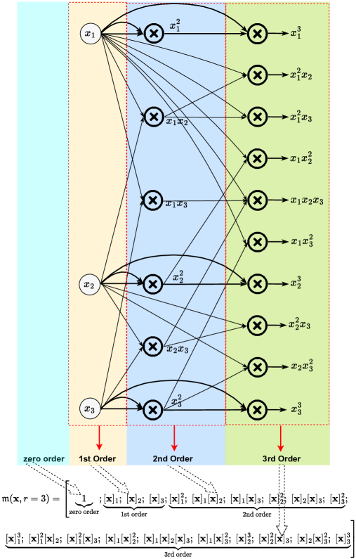
Figure 6: An example of Algorithm 1 in TensorFlow framework, where input ${\mathbf{x}}\in\mathbb{R}^{3}$.

The procedure of NN input augmentation is formally described by Algorithm 1, which aims to generate the vector of physical features (i.e., node representations) in form of polynomial function. The Lines 6–13 of Algorithm 1 guarantee that the generated node-representation vector embraces all the non-missing and non-redundant monomials of polynomial function. The Line 16 shows that Algorithm 1 finally stacks vector with one. This operation means a PhyN node will be assigned to be one, and the bias will be thus treated as link weight associated with the nodes. As an example shown in Figure 6, the nn input augmentation empowers PhyN to well capture core nonlinearities of physical quantities such as kinetic energy ($\triangleq\frac{1}{2}m{v^{2}}$) and aerodynamic drag force ($\triangleq\frac{1}{2}\rho{v^{2}}{C_{D}}A$), that drive the state dynamics of physical systems, and then represent or approxi-
mate physical knowledge in form of
the polynomial function.

Appendix E Physics-Model-Guided Neural Network Editing

Algorithm 2 Physics-Model-Guided Neural Network Editing

1:Input: Network type set $\mathbb{T}=\left\{{`\mathcal{Q}^{\prime},`\pi^{\prime}}\right\}$, knowledge sets $\mathbb{K}_{\mathcal{Q}}$ (31) and $\mathbb{K}_{\pi}$ (32), number of PhyNs ${p}_{\mathcal{Q}}$ and ${p}_{\mathcal{\pi}}$, origin input $\mathbf{x}$, augmentation orders ${r}_{\mathcal{Q}}$ and ${r}_{\mathcal{\pi}}$, model matrices $\mathbf{A}_{\mathcal{Q}}$ and $\mathbf{A}_{\pi}$, terminal output dimension $\text{len}(\mathbf{y})$.

2:Choose network type $\varpi\in\mathbb{T}$;

3:Specify augmentation order of the first PhyN: $r_{\left\langle 1\right\rangle}\leftarrow{r}_{\varpi}$;

4:for $t=1$ to $p_{\varpi}$ do

5:     if $t==1$  then

6:         Generate node-representation vector $\mathfrak{m}(\mathbf{x},r_{\left\langle 1\right\rangle})$ via Algorithm 1;

7:         Generate weight matrix: ${\mathbf{W}_{\left\langle 1\right\rangle}}$

8:         Generate knowledge matrix $\mathbf{K}_{\left\langle 1\right\rangle}$:  $[\mathbf{K}_{\left\langle 1\right\rangle}]_{i,j}\leftarrow\begin{cases}[\mathbf{A}_{\varpi}]_{i,j},&[\mathbf{A}_{\varpi}]_{i,j}\in\mathbb{K}_{\varpi}\\ 0,&\text{otherwise}\end{cases}$

9:         Generate weight-masking matrix $\mathbf{M}_{\left\langle 1\right\rangle}$:  $[\mathbf{M}_{\left\langle 1\right\rangle}]_{i,j}\leftarrow\begin{cases}0,&[\mathbf{A}_{{}_{\varpi}}]_{i,j}\in\mathbb{K}_{\varpi}\\ 1,&\text{otherwise}\end{cases}$

10:         Generate activation-masking vector $\mathbf{a}_{\left\langle 1\right\rangle}$:

$$\hskip 128.0374pt[\mathbf{a}_{\left\langle 1\right\rangle}]_{i}\leftarrow\begin{cases}0,&[\mathbf{M}_{\left\langle 1\right\rangle}]_{i,j}=0,\forall j\in\{1,\ldots,\text{len}(\mathfrak{m}(\mathbf{x},r_{\left\langle 1\right\rangle}))\}\\ 1,&\text{otherwise}\end{cases};$$

11:     else if $t>1$ then

12:         Generate weight matrix: ${\mathbf{W}_{\left\langle t\right\rangle}}$

13:         Generate node-representation vector $\mathfrak{m}(\mathbf{y}_{\left\langle t-1\right\rangle},r_{\left\langle t\right\rangle})$ via Algorithm 1

14:         Generate knowledge matrix $\mathbf{K}_{\left\langle t\right\rangle}$:

$$\hskip 51.21504pt\mathbf{K}_{\left\langle t\right\rangle}\leftarrow\left[\begin{gathered}\leavevmode\hbox to270.7pt{\vbox to68.29pt{\text{[drawing]}}}\end{gathered}\right]; \mathbf{O}_{(\text{len}(\mathbf{y}_{\left\langle t\right\rangle})-\text{len}(\mathbf{y}))\times\text{len}(\mathfrak{m}(\mathbf{y}_{\left\langle t-1\right\rangle},r_{\left\langle t\right\rangle}))} \mathbf{0}_{\text{len}(\mathbf{y})} \mathbf{I}_{\text{len}(\mathbf{y})} \mathbf{O}_{\text{len}(\mathbf{y})\times(\text{len}(\mathfrak{m}(\mathbf{y}_{\left\langle t-1\right\rangle},r_{\left\langle t\right\rangle}))-\text{len}(\mathbf{y})-1)} \mathbf{O}_{(\text{len}(\mathbf{y}_{\left\langle t\right\rangle})-\text{len}(\mathbf{y}))\times\text{len}(\mathfrak{m}(\mathbf{y}_{\left\langle t-1\right\rangle},r_{\left\langle t\right\rangle}))} \mathbf{0}_{\text{len}(\mathbf{y})} \mathbf{I}_{\text{len}(\mathbf{y})} \mathbf{O}_{\text{len}(\mathbf{y})\times(\text{len}(\mathfrak{m}(\mathbf{y}_{\left\langle t-1\right\rangle},r_{\left\langle t\right\rangle}))-\text{len}(\mathbf{y})-1)}$$ (75)

15:         Generate weight-masking matrix $\mathbf{M}_{\left\langle t\right\rangle}$:

$$\hskip 42.67912pt[\mathbf{M}_{\left\langle t\right\rangle}]_{i,j}\leftarrow\begin{cases}0,\!\!&\frac{{\partial[\mathfrak{m}(\mathbf{y}_{\left\langle t\right\rangle},r_{\left\langle t\right\rangle})]_{j}}}{{\partial[\mathfrak{m}(\mathbf{x},r_{\left\langle 1\right\rangle})]_{v}}}\!\neq\!0~{}\text{and}~{}[\mathbf{M}_{\left\langle 1\right\rangle}]_{i,v}\!=\!0,~{}v\!\in\!\{1,\dots,\text{len}(\mathfrak{m}(\mathbf{x},r_{\left\langle 1\right\rangle}))\}\\ 1,\!\!&\text{otherwise}\end{cases};$$

16:         Generate activation-masking vector $\mathbf{a}_{\left\langle t\right\rangle}\leftarrow\left[\mathbf{a}_{\left\langle 1\right\rangle};~{}\mathbf{1}_{\text{len}(\mathbf{y}_{\left\langle t\right\rangle})-\text{len}(\mathbf{y})}\right]$

17:     end if

18:     Generate uncertainty matrix $\mathbf{U}_{\left\langle t\right\rangle}\leftarrow\mathbf{M}_{\left\langle t\right\rangle}\odot{\mathbf{W}_{\left\langle t\right\rangle}}$

19:     Compute output: $\mathbf{y}_{\left\langle t\right\rangle}\leftarrow\mathbf{K}_{\left\langle t\right\rangle}\cdot\mathfrak{m}(\mathbf{y}_{\left\langle t-1\right\rangle},r_{\left\langle t\right\rangle})+\mathbf{a}_{\left\langle t\right\rangle}\odot\text{act}\left({\mathbf{U}_{\left\langle t\right\rangle}\cdot\mathfrak{m}\left({\mathbf{y}_{\left\langle t-1\right\rangle},r_{\left\langle t\right\rangle}}\right)}\right)$

20:end for

21:Output: $\widehat{\mathbf{y}}\leftarrow\mathbf{y}_{\left\langle p\right\rangle}$

Remark E.1 (Activation Editing).

For the edited weight matrix $\mathbf{W}_{\left\langle t\right\rangle}$, if its entries in the same row are all in the knowledge set, the associated activation should be inactivate. Otherwise, the BNN cannot strictly preserve the available physical knowledge due to the extra nonlinear mappings induced by the activation functions. This thus motivates the physics-knowledge preserving computing, i.e., the Line 19 of Algorithm 2. Figure 7 summarizes the flowchart of NN editing in a single PhN layer:

• Given the node-representation vector from Algorithm 1, the original (fully-connected) weight matrix is edited via link editing to embed assigned physical knowledge, resulting in $\mathbf{W}_{\left\langle t\right\rangle}$.

• The edited weight matrix ${\mathbf{W}_{\left\langle t\right\rangle}}$ is separated into knowledge matrix $\mathbf{K}_{\left\langle t\right\rangle}$ and uncertainty matrix $\mathbf{U}_{\left\langle t\right\rangle}$, such that ${\mathbf{W}_{\left\langle t\right\rangle}}=\mathbf{K}_{\left\langle t\right\rangle}+\mathbf{U}_{\left\langle t\right\rangle}$. Specifically, the $\mathbf{K}_{\left\langle t\right\rangle}$, generated in Lines 8 and 14 of Algorithm 2, includes all the parameters in knowledge set. While the $\mathbf{M}_{\left\langle t\right\rangle}$, generated in Lines 9 and 15, is used to generate uncertainty matrix $\mathbf{U}_{\left\langle t\right\rangle}$ (see Line 18) to include all the parameters excluded from knowledge set, through freezing the parameters (from knowledge set) of $\mathbf{W}_{\left\langle t\right\rangle}$ to zeros.

• The $\mathbf{K}_{\left\langle t\right\rangle}$, $\mathbf{M}_{\left\langle t\right\rangle}$ and activation-masking vector $\mathbf{a}_{\left\langle t\right\rangle}$ (generated in Lines 10 and 16) are used by activation editing for the physical-knowledge-preserving computing of output in each PhyN layer. The function of $\mathbf{a}_{\left\langle t\right\rangle}$ is to avoid the extra mapping (induced by activation) that prior physical knowledge does not include.

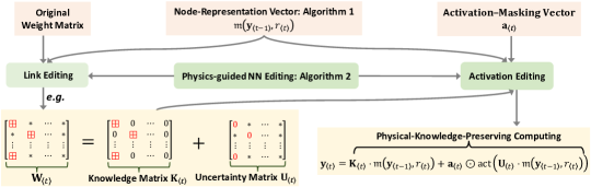
Figure 7: Flowchart of NN editing in single PhyN layer, where $\boxplus$ and $*$ denote a parameter included in and excluded from knowledge set, respectively.

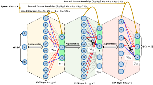
Figure 8: Example of NN editing, i.e., Algorithm 2. (i) Parameters excluded from knowledge set are formed by the grey links, the parameters included in knowledge set are formed by the red and blue links. (ii) Cutting black links is to avoid spurious correlations, otherwise, the links can lead to violation of physical knowledge.

Remark E.2 (Knowledge Preserving and Passing).

The flowchart of NN editing operating in BNN, i.e., cascade PhyNs is depicted in Figure 8. The Lines 5-9 of Algorithm 2 means that $\mathbf{A}_{\varpi}=\mathbf{K}_{\left\langle 1\right\rangle}+\mathbf{M}_{\left\langle 1\right\rangle}\odot\mathbf{A}_{\varpi}$, leveraging which and the setting $r_{\left\langle 1\right\rangle}=r_{\varpi}$, the ground-truth model (29) or (30) can be rewritten as

$$\mathbf{y} =(\mathbf{K}_{\left\langle 1\right\rangle}+\mathbf{M}_{\left\langle 1\right\rangle}\odot\mathbf{A}_{\varpi})\cdot\mathfrak{m}(\mathbf{x},r)+\mathbf{f}(\mathbf{x})$$

$$=\mathbf{K}_{\left\langle 1\right\rangle}\cdot\mathfrak{m}(\mathbf{x},r_{\left\langle 1\right\rangle})+(\mathbf{M}_{\left\langle 1\right\rangle}\odot\mathbf{A}_{\varpi})\cdot\mathfrak{m}(\mathbf{x},r_{\left\langle 1\right\rangle})+\mathbf{f}(\mathbf{x}).$$ (76)

where $\mathbf{y}=\mathcal{Q}\left(\mathbf{s}(k),\mathbf{a}_{\text{drl}}(k)\right)$ or $\pi\left(\mathbf{s}(k)\right)$, and $\mathbf{x}=\left[\mathbf{s}(k);\mathbf{a}_{\text{drl}}(k)\right]$ or $\mathbf{s}(k)$, depending on $\varpi$. We obtain from the Line 19 of Algorithm 2 that the output of the first PhyN layer is

$$\mathbf{y}_{\left\langle 1\right\rangle}=\mathbf{K}_{\left\langle 1\right\rangle}\cdot\mathfrak{m}(\mathbf{x},r_{\left\langle 1\right\rangle})+\mathbf{a}_{\left\langle 1\right\rangle}\odot\text{act}\left({\mathbf{U}_{\left\langle 1\right\rangle}\cdot{\mathfrak{m}}\left({\mathbf{x},r_{\left\langle 1\right\rangle}}\right)}\right).$$ (77)

Recalling that $\mathbf{K}_{\left\langle 1\right\rangle}$ includes all the entries of $\mathbf{A}_{\varpi}$ while the $\mathbf{U}_{\left\langle 1\right\rangle}$ includes remainders, we conclude from (76) and (77) that the available physical knowledge pertaining to the ground-truth model has been embedded to the first PhyN layer. As Figure 8 shows the embedded knowledge shall be passed down to the remaining cascade PhyNs and preserved therein, such that the end-to-end BNN model can strictly with the physical knowledge. This knowledge passing is achieved by the block matrix $\mathbf{K}_{\left\langle p\right\rangle}$ generated in Line 14, due to which, the output of $t$-th PhyN layer satisfies

$$\!\![\mathbf{y}_{\left\langle t\right\rangle}]_{1:\text{len}(\mathbf{y})}\!=\!\underbrace{\mathbf{K}_{\left\langle 1\right\rangle}\cdot\mathfrak{m}(\mathbf{x},r_{\left\langle 1\right\rangle})}_{\text{knowledge passing}}\!+\!\underbrace{[\mathbf{a}_{\left\langle t\right\rangle}\odot\text{act}\!\left({\mathbf{U}_{\left\langle t\right\rangle}\cdot{\mathfrak{m}}({\mathbf{y}_{\left\langle t-1\right\rangle},r_{\left\langle t\right\rangle}})}\right)]_{1:\text{len}(\mathbf{y})}}_{\text{knowledge preserving}},~{}\forall t\!\in\!\{2,\ldots,p\}.$$ (78)

Meanwhile, the $\mathbf{U}_{\left\langle t\right\rangle}=\mathbf{M}_{\left\langle t\right\rangle}\odot{\mathbf{W}_{\left\langle t\right\rangle}}$ means the masking matrix $\mathbf{M}_{\left\langle t\right\rangle}$ generated in Line 15 is to remove the spurious correlations in the cascade PhyNs, which is depicted by the cutting link operation in Figure 8.

Appendix F Proof of Theorem 4.1

Let us first consider the first PhyN layer, i.e., the case $t=1$. The Line 8 of Algorithm 2 means that the knowledge matrix $\mathbf{K}_{\left\langle 1\right\rangle}$ includes all the known model-substructure parameters, whose corresponding entries in the masking matrix $\mathbf{M}_{\left\langle 1\right\rangle}$ (generated in the Line 9 of Algorithm 2) are frozen to be zeros. Consequently, both $\mathbf{M}_{\left\langle 1\right\rangle}\odot\mathbf{A}_{\varpi}$ and $\mathbf{U}_{\left\langle 1\right\rangle}=\mathbf{M}_{\left\langle 1\right\rangle}\odot\mathbf{W}_{\left\langle 1\right\rangle}$ excludes all the known model-substructure parameters (included in $\mathbf{K}_{\left\langle 1\right\rangle}$). We thus conclude that $\mathbf{M}_{\left\langle 1\right\rangle}\odot\mathbf{A}_{\varpi}\cdot\mathfrak{m}(\mathbf{x},r_{\left\langle 1\right\rangle})+\mathbf{f}(\mathbf{x})$ in the ground-truth model (76) and $\mathbf{a}_{\left\langle 1\right\rangle}\odot\text{act}\left(\mathbf{U}_{\left\langle 1\right\rangle}\cdot{\mathfrak{m}}\left(\mathbf{x},r_{\left\langle 1\right\rangle}\right)\right)$ in the output computation in Line 21 are independent of the term $\mathbf{K}_{\left\langle 1\right\rangle}\cdot\mathfrak{m}(\mathbf{x},r_{\left\langle 1\right\rangle})$. Moreover, the activation-masking vector (generated in Line 10 of Algorithm 2) indicates that the activation function corresponding to the output’s $i$-th entry is inactive, if the all the entries in the $i$-th row of masking matrix are zeros (implying all the entries in the $i$-th row of weight matrix are included in the knowledge set $\mathbb{K}_{\varpi}$). Finally, we arrive in the conclusion that the input/output of the first PhyN layer strictly complies with the available physical knowledge pertaining to the ground truth (76), i.e., if the $[\mathbf{A}_{\varpi}]_{i,j}\in\mathbb{K}_{\varpi}$, the $\frac{{\partial{[\mathbf{y}_{\left\langle 1\right\rangle}]_{i}}}}{{\partial[{\mathfrak{m}}\left({\mathbf{x},r_{\varpi}}\right)]_{j}}}\equiv{[\mathbf{A}_{\varpi}]_{i,j}}$ always hold.

We next consider the remaining PhyN layers. Considering the Line 19 Algorithm 2, we have

$$[\mathbf{y}_{\left\langle p\right\rangle}]_{1:\text{len}(\mathbf{y})}$$

$$=[\mathbf{K}_{\left\langle p\right\rangle}\cdot\mathfrak{m}(\mathbf{y}_{\left\langle p-1\right\rangle},r_{\left\langle p\right\rangle})]_{1:\text{len}(\mathbf{y})}+[\mathbf{a}_{\left\langle p\right\rangle}\odot\text{act}\!\left({\mathbf{U}_{\left\langle p\right\rangle}\cdot{\mathfrak{m}}({\mathbf{y}_{\left\langle p-1\right\rangle},r_{\left\langle p\right\rangle}})}\right)]_{1:\text{len}(\mathbf{y})}$$

$$=\mathbf{I}_{\text{len}(\mathbf{y})}\cdot[\mathfrak{m}(\mathbf{y}_{\left\langle p-1\right\rangle},r_{\left\langle p\right\rangle})]_{2:(\text{len}(\mathbf{y})+1)}+[\mathbf{a}_{\left\langle p\right\rangle}\odot\text{act}\!\left({\mathbf{U}_{\left\langle p\right\rangle}\cdot{\mathfrak{m}}({\mathbf{y}_{\left\langle p-1\right\rangle},r_{\left\langle p\right\rangle}})}\right)]_{1:\text{len}(\mathbf{y})}$$ (79)

$$=\mathbf{I}_{\text{len}(\mathbf{y})}\cdot[\mathbf{y}_{\left\langle p-1\right\rangle}]_{1:\text{len}(\mathbf{y})}+[\mathbf{a}_{\left\langle p\right\rangle}\odot\text{act}\!\left({\mathbf{U}_{\left\langle p\right\rangle}\cdot{\mathfrak{m}}({\mathbf{y}_{\left\langle p-1\right\rangle},r_{\left\langle p\right\rangle}})}\right)]_{1:\text{len}(\mathbf{y})}$$ (80)

$$=[\mathbf{y}_{\left\langle p-1\right\rangle}]_{1:\text{len}(\mathbf{y})}+[\mathbf{a}_{\left\langle p\right\rangle}\odot\text{act}\!\left({\mathbf{U}_{\left\langle p\right\rangle}\cdot{\mathfrak{m}}({\mathbf{y}_{\left\langle p-1\right\rangle},r_{\left\langle p\right\rangle}})}\right)]_{1:\text{len}(\mathbf{y})}$$

$$=[\mathbf{K}_{\left\langle p-1\right\rangle}\cdot\mathfrak{m}(\mathbf{y}_{\left\langle p-2\right\rangle},r_{\left\langle p-1\right\rangle})]_{1:\text{len}(\mathbf{y})}+[\mathbf{a}_{\left\langle p\right\rangle}\odot\text{act}\!\left({\mathbf{U}_{\left\langle p\right\rangle}\cdot{\mathfrak{m}}({\mathbf{y}_{\left\langle p-1\right\rangle},r_{\left\langle p\right\rangle}})}\right)]_{1:\text{len}(\mathbf{y})}$$

$$=\mathbf{I}_{\text{len}(\mathbf{y})}\cdot[\mathfrak{m}(\mathbf{y}_{\left\langle p-2\right\rangle},r_{\left\langle p-1\right\rangle})]_{2:(\text{len}(\mathbf{y})+1)}+[\mathbf{a}_{\left\langle p\right\rangle}\odot\text{act}\!\left({\mathbf{U}_{\left\langle p\right\rangle}\cdot{\mathfrak{m}}({\mathbf{y}_{\left\langle p-1\right\rangle},r_{\left\langle p\right\rangle}})}\right)]_{1:\text{len}(\mathbf{y})}$$

$$=\mathbf{I}_{\text{len}(\mathbf{y})}\cdot[\mathbf{y}_{\left\langle p-2\right\rangle}]_{1:\text{len}(\mathbf{y})}+[\mathbf{a}_{\left\langle p\right\rangle}\odot\text{act}\!\left({\mathbf{U}_{\left\langle p\right\rangle}\cdot{\mathfrak{m}}({\mathbf{y}_{\left\langle p-1\right\rangle},r_{\left\langle p\right\rangle}})}\right)]_{1:\text{len}(\mathbf{y})}$$

$$=[\mathbf{y}_{\left\langle p-2\right\rangle}]_{1:\text{len}(\mathbf{y})}+[\mathbf{a}_{\left\langle p\right\rangle}\odot\text{act}\!\left({\mathbf{U}_{\left\langle p\right\rangle}\cdot{\mathfrak{m}}({\mathbf{y}_{\left\langle p-1\right\rangle},r_{\left\langle p\right\rangle}})}\right)]_{1:\text{len}(\mathbf{y})}$$

$$=\ldots$$

$$=[\mathbf{y}_{\left\langle 1\right\rangle}]_{1:\text{len}(\mathbf{y})}+[\mathbf{a}_{\left\langle p\right\rangle}\odot\text{act}\!\left({\mathbf{U}_{\left\langle p\right\rangle}\cdot{\mathfrak{m}}({\mathbf{y}_{\left\langle p-1\right\rangle},r_{\left\langle p\right\rangle}})}\right)]_{1:\text{len}(\mathbf{y})}$$

$$=[\mathbf{K}_{\left\langle 1\right\rangle}\cdot\mathfrak{m}(\mathbf{x},r_{\left\langle 1\right\rangle})]_{1:\text{len}(\mathbf{y})}+[\mathbf{a}_{\left\langle p\right\rangle}\odot\text{act}\!\left({\mathbf{U}_{\left\langle p\right\rangle}\cdot{\mathfrak{m}}({\mathbf{y}_{\left\langle p-1\right\rangle},r_{\left\langle p\right\rangle}})}\right)]_{1:\text{len}(\mathbf{y})}$$

$$=\mathbf{K}_{\left\langle 1\right\rangle}\cdot\mathfrak{m}(\mathbf{x},r_{\left\langle 1\right\rangle})+[\mathbf{a}_{\left\langle p\right\rangle}\odot\text{act}\!\left({\mathbf{U}_{\left\langle p\right\rangle}\cdot{\mathfrak{m}}({\mathbf{y}_{\left\langle p-1\right\rangle},r_{\left\langle p\right\rangle}})}\right)]_{1:\text{len}(\mathbf{y})},$$ (81)

where (79) and (80) are obtained from their previous steps via considering the structure of block matrix $\mathbf{K}_{\left\langle t\right\rangle}$ (generated in the Line 14 of Algorithm 2) and the formula of augmented monomials: $\mathfrak{m}(\mathbf{y},r)=\left[1;~{}\mathbf{y};~{}[\mathfrak{m}({\mathbf{y},r})]_{(\text{len}(\mathbf{y})+2):\text{len}(\mathfrak{m}(\mathbf{y},r))}\right]$ (generated via Algorithm 2). The remaining iterative steps follow the same path.

The training loss function is to push the terminal output of Algorithm 2 to approximate the real output $\mathbf{y}$, which in light of (81) yields

$$\widehat{\mathbf{y}} =\mathbf{K}_{\left\langle 1\right\rangle}\cdot\mathfrak{m}(\mathbf{x},r_{\left\langle 1\right\rangle})+[\mathbf{a}_{\left\langle p\right\rangle}\odot\text{act}\!\left({\mathbf{U}_{\left\langle p\right\rangle}\cdot{\mathfrak{m}}({\mathbf{y}_{\left\langle p-1\right\rangle},r_{\left\langle p\right\rangle}})}\right)]_{1:\text{len}(\mathbf{y})}$$

$$=\mathbf{K}_{\left\langle 1\right\rangle}\cdot\mathfrak{m}(\mathbf{x},r_{\left\langle 1\right\rangle})+\mathbf{a}_{\left\langle p\right\rangle}\odot\text{act}\!\left({\mathbf{U}_{\left\langle p\right\rangle}\cdot{\mathfrak{m}}({\mathbf{y}_{\left\langle p-1\right\rangle},r_{\left\langle p\right\rangle}})}\right),$$ (82)

where (82) from its previous step is obtained via considering the fact $\text{len}(\widehat{\mathbf{y}})=\text{len}(\mathbf{y})=\text{len}(\mathbf{y}_{\left\langle p\right\rangle})$. Meanwhile, the condition of generating weight-masking matrix in Line 15 of Algorithm 2 removes all the node-representations’ connections with the known model-substructure parameters included in $\mathbf{K}_{\left\langle 1\right\rangle}$. Therefore, we can conclude that in the terminal output computation (82), the term $\mathbf{a}_{\left\langle p\right\rangle}\odot\text{act}\!\left({\mathbf{U}_{\left\langle p\right\rangle}\cdot{\mathfrak{m}}({\mathbf{y}_{\left\langle p-1\right\rangle},r_{\left\langle p\right\rangle}})}\right)$ does not have influence on the computing of knowledge term $\mathbf{K}_{\left\langle 1\right\rangle}\cdot\mathfrak{m}(\mathbf{x},r_{\left\langle 1\right\rangle})$. Thus, the Algorithm 2 strictly embeds and preserves the available knowledge pertaining to the physics model of ground truth.

Appendix G Experiment: Car-Pole Inverted Pendulum

G.1 Model and Safety Knowledge

To have the model-based safe control, the first step is to obtain system matrix $\mathbf{A}$ and control structure matrix $\mathbf{B}$ in real plant (1). In other words, the available model knowledge pertaining to real plant (1) is a linear model trying to approximate the real nonlinear system:

$$\bar{\mathbf{s}}(k+1)={\mathbf{A}}\cdot\bar{\mathbf{s}}(k)+{\mathbf{B}}\cdot\bar{\mathbf{a}}(k),~{}~{}~{}~{}k\in\mathbb{N}.$$ (83)

We refer to the dynamics model of inverted pendulum described in [16] and consider the approximations $\cos\theta\approx 1$, $\sin\theta\approx\theta$ and ${\omega^{2}}\sin\theta\approx 0$ for obtaining

$$\mathbf{A}=\left[{\begin{array}[]{*{20}{c}}1&{0.0333}&0&0\\ 0&1&{-0.0565}&0\\ 0&0&1&{0.0333}\\ 0&0&{0.8980}&1\end{array}}\right],~{}~{}~{}~{}~{}\mathbf{B}=\left[0~{}~{}0.0334~{}~{}0~{}~{}-0.0783\right]^{\top}.$$ (88)

Considering the conditions in (33), we obtain the safety set defined in (2), where

$$\mathbf{s}=\left[\!\begin{array}[]{l}x\\ v\\ \theta\\ \omega\end{array}\!\right]\!,~{}~{}\mathbf{D}=\left[\!{\begin{array}[]{*{20}{c}}1\!&\!0\!&\!0\!&\!0\\ 0\!&\!0\!&\!1\!&\!0\\ \end{array}}\!\right]\!,~{}~{}\mathbf{v}=\left[\!\begin{array}[]{l}0\\ 0\end{array}\!\right]\!,~{}~{}\overline{\mathbf{v}}=\left[\!\begin{array}[]{l}0.9\\ 0.8\end{array}\!\right]\!,~{}~{}\underline{\mathbf{v}}=\left[\!\begin{array}[]{l}-0.9\\ -0.8\end{array}\!\right]\!,~{}~{}\mathbf{C}=1,~{}~{}\mathbf{z}=0,$$ (101)

$$\overline{\mathbf{v}}=16,~{}~{}\underline{\mathbf{z}}=-16,$$ (102)

based on which, according to (38)–(40) we have:

$$\mathbf{d}=\left[\!\begin{array}[]{l}-1\\ -1\end{array}\!\right]\!,~{}~{}~{}\overline{\Lambda}=\underline{\Lambda}=\left[\!{\begin{array}[]{*{20}{c}}0.9&0\\ 0&0.8\end{array}}\!\right]$$ (107)

from which and $\mathbf{D}$ given in (102), we then have

$$\overline{\mathbf{D}}=\frac{{\mathbf{D}}}{\overline{\Lambda}}=\underline{\mathbf{D}}=\frac{{\mathbf{D}}}{\underline{\Lambda}}=\left[\!{\begin{array}[]{*{20}{c}}\frac{10}{9}\!&\!0\!&\!0\!&\!0\\ 0\!&\!0\!&\!\frac{5}{4}\!&\!0\\ \end{array}}\!\right].$$ (110)

G.2 Model-Based Design Solutions

With the knowledge given in (107) and (110), the matrices $\mathbf{F}$ and $\mathbf{P}$ are ready to be obtained from inequalities (19) and (25). Meanwhile, we are interested in a solution that can maximize the safety envelope (18). Furthermore, noticing the volume of a safety envelope (18) is proportional to $\sqrt{\det\left({\mathbf{P}^{-1}}\right)}$, the considered problem is thus a typical analytic centering problem [43]:

$$\mathop{\min}\limits_{{\mathbf{Q}},~{}{\mathbf{R}}}\left\{{\log\det\left({\mathbf{Q}^{-1}}\right)}\right\}=\mathop{\max}\limits_{{\mathbf{Q}},~{}{\mathbf{R}}}\left\{{\log\det\left({\mathbf{P}^{-1}}\right)}\right\},~{}~{}~{}\text{subject to}~{}\eqref{set5}~{}\text{and}~{}\eqref{th1}$$ (111)

from which via the CVXPY toolbox [13] in Python, with $\alpha=0.98$ and $\beta=250$, we obtain

$$\mathbf{Q} =\left[{\begin{array}[]{*{20}{c}}0.66951866&-0.69181711&-0.27609583&0.55776279\\ -0.69181711&9.86247186&0.1240829&-12.4011146\\ -0.27609583&0.1240829&0.66034399&-2.76789607\\ 0.55776279&-12.4011146&-2.76789607&32.32280039\end{array}}\right],$$ (116)

$$\mathbf{R} =\left[{\begin{array}[]{*{20}{c}}-6.40770185&-18.97723676&6.10235911&31.03838284\end{array}}\right],$$ (118)

based on which, we then have

$$\mathbf{P} =\mathbf{Q}^{-1}=\left[{\begin{array}[]{*{20}{c}}4.6074554&1.49740096&5.80266046&0.99189224\\ 1.49740096&0.81703147&2.61779592&0.51179642\\ 5.80266046&2.61779592&11.29182733&1.87117709\\ 0.99189224&0.51179642&1.87117709&0.37041435\end{array}}\right],$$ (123)

$$\mathbf{F} =\mathbf{R}\cdot\mathbf{P}=\left[{\begin{array}[]{*{20}{c}}8.25691599&6.76016534&40.12484514&6.84742553\end{array}}\right],$$ (125)

$$\overline{\mathbf{A}} =\mathbf{A}+{\mathbf{B}}\cdot{\mathbf{F}}=\left[{\begin{array}[]{*{20}{c}}1&0.03333333&0&0\\ 0.27592037&1.22590363&1.2843559&0.2288196\\ 0&0&1&0.03333333\\ -0.64668827&-0.52946156&-2.24458365&0.46370415\end{array}}\right].$$ (130)

With these solutions, we are able to deliver model-based control commands and safety-embedded reward.

G.3 Failure: Sole Model-Based Control

The trajectories of the inverted pendulum under sole model-based control, i.e., $\mathbf{a}(k)=\mathbf{a}_{\text{phy}}(k)=\mathbf{F}\cdot\mathbf{s}(k)$, are shown in Figure 10, where system initial condition lies in the safety envelope, i.e., $\mathbf{s}(1)\in{\Omega}$. Figure 10 shows the sole model-based control commands cannot stabilize the inverted pendulum and cannot guarantee its safety. This failure is due to a large model mismatch between the simplified linear model (83) and the real nonlinear system. While Figure 4 shows the Phy-DRL successfully overcomes the large model mismatch and renders the system safe.

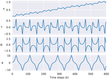
Figure 10: System trajectories of the inverted pendulum: unstable and unsafe.

G.4 Configurations: Networks and Training

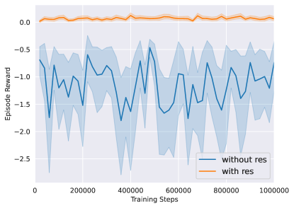
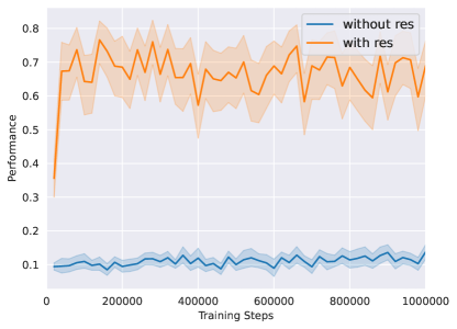
Figure 11: Phy-DRL (i.e., CLF reward + residual control) v.s. purely data-driven DRL (CLF reward).

In this case study, the control goal is to stabilize the pendulum at the equilibrium $\mathbf{s}^{*}=[x^{*},v^{*},\theta^{*},\omega^{*}]^{\top}=[0,0,0,0]^{\top}$. We convert the measured angle $\theta$ into $\sin(\theta)$ and $\cos(\theta)$ to simplify the learning process. Therefore, the observation space can be expressed as

$$\mathbf{o}=[x,~{}v,~{}\sin(\theta),~{}\sin(\theta),~{}\omega]^{\top}.$$

We added a terminal condition to the training episode that stops the running of the inverted pendulum when a violation of safety occurs, depicted as follows:

$$\beta(\mathbf{s}(k))=\begin{cases}1,&\text{if $|x(k)|\geq 0.9$ or $|\theta(k)|\geq 0.8$}\\ 0,&\text{otherwise.}\end{cases}$$

Specifically, the operation of the inverted pendulum is terminated if either its cart position or pendulum angle exceeds the safety bounds or the pendulum falls down. During training, we reset episodes to a random initial state if the maximum step of system running is reached, or $\beta(\mathbf{s}(k))=1$.

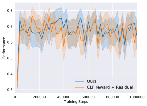
Figure 12: System performances in training: Our Phy-DRL and the Phy-DRL but using CLF reward.

The development of Phy-DRL is based on DDPG algorithm. The actor and critic networks in the DDPG algorithm are both implemented as a Multi-Layer Perceptron (MLP) with four fully connected layers. The output dimensions of both critic and actor networks are 256, 128, 64, and 1, respectively. The activation functions of the first three neural layers are ReLU, while the output of the last layer is the Tanh function for the actor network and Linear for the critic network. The input of the critic network is $[\mathbf{o};\mathbf{u}]$, while the input of the actor network is $\mathbf{o}$.

G.5 Influences on Training

We now consider two different Phy-DRL architectures: 1) residual control + CLF reward (proposed in [50]: $\mathcal{R}(\cdot)=\mathbf{s}^{\top}(k)\cdot\mathbf{P}\cdot\mathbf{s}(k)-{\mathbf{s}^{\top}(k+1)}\cdot\mathbf{P}\cdot\mathbf{s}(k+1)+w(\mathbf{s}(k),\mathbf{a}(k))$), and 2) residual control + our proposed reward (20), where $w(\mathbf{s}(k),\mathbf{a}_{\text{drl}}(k))=-\mathbf{a}_{\text{drl}}^{2}(k)$. The training trajectories of episode reward and system performance of the former Phy-DRL v.s. the purely data-driven DRL (using CLF reward) are shown in Figure 11. The training trajectories of episode reward and system performance of the two Phy-DRLs are presented in Figure 12. Observing the comparisons in Figures 10–12 and 3, we have very interesting discoveries. Specifically, although the sole model-based control cannot achieve the safe control mission, it guides the exploration of DRL agents during training and regulates the behavior of data-driven DRL controller, such that both Phy-DRLs feature significantly enlarged episode reward and much faster training. Theoretically, it is because of the model-based design in the residual control component, that our proposed Phy-DRL can exhibit mathematically-provable safety and stability guarantees.

Appendix H Experiment: Quadruped Robot

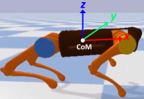
Figure 13: Quadruped robot: 3D single rigid-body model.

H.1 Model-Based Design

The dynamics model of the robot is based on a single rigid body subject to forces at the contact patches [12]. Referring to Figure 13, the considered robot dynamics is characterized by the position of the body center of mass (CoM) $\mathbf{p}=[p_{x};p_{y};p_{z}]\in\mathbb{R}^{3}$, the CoM velocity $\mathbf{v}\triangleq\dot{\mathbf{p}}\in\mathbb{R}^{3}$, the Euler angles $\widetilde{\mathbf{e}}=[\phi;\theta;\psi]\in\mathbb{R}^{3}$ with $\phi$, $\theta$ and $\psi$ being roll, pitch and yaw angels, respectively, and the angular velocity in the velocity in world coordinates $\mathbf{w}\in\mathbb{R}^{3}$. Before presenting the body dynamics, we introduce the order of foot states $\{\text{Left Front (LF)},\text{Right Front (RF)},\text{Left Rear (LR)},\text{Right Rear (RR)}\}$, based on which we define the following two footsteps for describing the trotting behavior of quadruped robots:

$$\text{Step}_{1}\triangleq\{\text{LF}\!=\!1,\text{RF}\!=\!0,\text{LR}\!=\!0,\text{RR}\!=\!1\},~{}~{}~{}\text{Step}_{2}\triangleq\{\text{LF}\!=\!0,\text{RF}\!=\!1,\text{LR}\!=\!1,\text{RR}\!=\!0\},$$ (131)

where ‘0’ indicates that the corresponding foot is a stance, and ‘1’ denotes otherwise. The considered walking controller lifts one foot at a time by switching between four stepping primitives in the order:

$$\text{Step}_{1}\to\text{Step}_{2}\to\text{Step}_{1}\to\text{Step}_{2}\to\text{Step}_{1}\to\text{Step}_{2}\to\text{Step}_{1}\to\text{Step}_{2}\to\ldots\to\text{repeating}\to\dots$$

Like [10], the control commands from Phy-DRL will be the desired positional acceleration $\ddot{\mathbf{p}}$ and rotational acceleration $\ddot{\widetilde{\mathbf{e}}}$. The acceleration output will be converted to the torque control for the low-level motors. This experiment mainly focuses on the validation of the knowledge-enhanced critic and actor networks. So, the Phy-DRL directly adopts the PD controller proposed in [10] as the model-based controller. The considered reward is constructed according to matrix $\mathbf{P}$ computed according to (111):

$$\mathcal{R}({\mathbf{s},\mathbf{a}_{\text{drl}}})=0.00018\cdot([\mathbf{w}]^{2}_{1}+[\mathbf{w}]^{2}_{2}+[\mathbf{w}]^{2}_{3}+[\mathbf{v}]^{2}_{2}+[\mathbf{v}]^{2}_{3})+[\mathbf{v}]^{2}_{1}.$$

H.2 Comparisons with Purely Data-Driven DRL

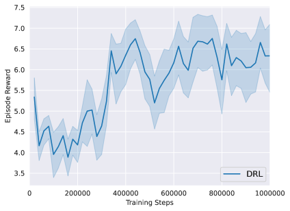
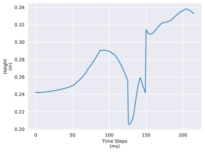
Figure 14: Purely data-driven DRL

In this quadruped robot study, the control goal is to track the reference velocity $\dot{p_{x}}^{*}=1.0$ m/s and maintain the desired height $p_{z}=0.24$ m on a low-friction road. The state of the quadruped robot consists of 12 elements $\mathbf{s}=[\mathbf{p};~{}\mathbf{v};~{}\widetilde{\mathbf{e}};~{}\mathbf{w}]$. To reduce the learning space, we calculate the relative distance between the current state $\mathbf{s}$ and the reference state $\mathbf{s}^{*}$ to form the observation space, as follows:

$$\mathbf{o}=[\mathbf{p}-\mathbf{p}^{*},\dot{\mathbf{p}}-\dot{\mathbf{p}}^{*},\widetilde{\mathbf{e}}-\widetilde{\mathbf{e}}^{*},\dot{\widetilde{\mathbf{e}}}-\dot{\widetilde{\mathbf{e}}}^{*}].$$

We added a terminal condition to the training episode when the robot’s roll or pitch exceeds 30 degrees. During training, we reset episodes to the origin of the world coordinate if the maximum step of system running is reached, or the robot reaches the termination state.

Typically, purely data-driven based approach would take very long time to interact with the environment to learn a good policy. For example, the work [25] takes 1.2 billion steps for training. To build the baseline for the comparison, we implement a purely data-driven training with the reward function designed from a data-efficient framework in [Smith et al. arXiv:2208.07860.], depicted as the following:

$$r(s,a)=r_{v}(s,a)-0.1\ddot{\psi}^{2}$$

where $\ddot{\psi}$ is an angular yaw velocity and

$$r_{v}(s,a)=\begin{cases}1,&\text{for }\dot{p_{x}}\in[\dot{p_{x}}^{*},2\dot{p_{x}}^{*}]\\ 0,&\text{for }\dot{p_{x}}\in(-\infty,-\dot{p_{x}}^{*}]\cup[4\dot{p_{x}}^{*},\infty)\\ 1-\frac{|\dot{p_{x}}-\dot{p_{x}}^{*}|}{2\dot{p_{x}}^{*}},&\text{otherwise.}\end{cases}$$

where $\dot{p_{x}}^{*}$ is the target velocity, while $\dot{p_{x}}$ is a forward linear velocity in the robot frame.

We leverage the DDPG algorithm again for training the purely data-driven DRL and our Phy-DRL. The actor and critic networks in the DDPG algorithm are both implemented as a Multi-Layer Perceptron (MLP) with four fully connected layers. The output dimensions of hidden layers of critic and actor networks are 128, 128, and 128. The final dimension of the output layer is 1 for the critic network, denoting the $Q$ value, and 6 for the actor network, denoting the acceleration output. The activation functions of the first three neural layers are ReLU, while the output of the last layer is the Tanh function for the actor network and Linear for the critic network. The input of the critic network is $[\mathbf{o};\mathbf{u}]$, while the input of the actor network is $\mathbf{o}$.

The purely data-driven DRL is trained for $10^{6}$ steps. The trajectories of the training episode reward and the robot height of a trained model are shown in Figure 14, which in conjunction with Figure 5, show that training for $10^{6}$ steps, the purely data-driven DRL cannot achieve the control mission while the Phy-DRL successfully makes it.

H.3 Knowledge-Enhanced Critic Network

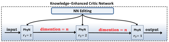
Figure 15: Considered knowledge-enhanced critic network.

Table 2: Model Parameters

	Layer 1		Layer 2		Layer 3		Layer 4
Model ID	#weights	#bias	#Weights	#bias	#weights	#bias	#weights	#bias	#parameter sum
FC MLP	$2304$	$128$	$16384$	128	$16384$	$128$	$128$	$1$	35585
KN 2	$342$	$2$	$10$	$2$	$2$	$1$	$-$	$-$	359
KN 3	$513$	$3$	$27$	$3$	$3$	$1$	$-$	$-$	550
KN 5	$855$	$5$	$100$	$5$	$5$	$1$	$-$	$-$	971

Our proposed reward and the formula (17) imply that the Q-value does not include any odd-order monomials, and the critic network shall strictly comply with this knowledge. This knowledge compliance can be achieved via our proposed NN editing. The architecture of the resulting knowledge-enhanced critic network in this example is shown in Figure 15, where the PhN architecture is given in Figure 2 (b). We compare the performance of knowledge-enhanced critic networks with fully-connected MLP (FC MLP) used in Section H.2. Figure 15 shows that different critic networks can be obtained by changing the output dimensions $n$. We here consider three models: knowledge-enhanced critic network with $n=2$ (KN 2), knowledge-enhanced critic network with $n=3$ (KN 3), and knowledge-enhanced critic network with $n=5$ (KN 5). The parameter numbers of all network models are summarized in Table 2.

The trajectories of episode reward of the four models are shown in Figure 16, which in conjunction with Table (2), show that except for the smallest network, i.e., KN 2, the knowledge-enhanced critic network, having a significantly small number of parameters (Models KN 3 and KN 5), can reach the similar performance (viewed from episode reward) of FC MLP having a number of parameters. This, on the other hand, means the knowledge-enhanced critic network can avoid significant spurious correlations via NN editing.

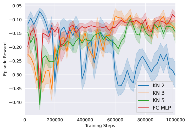
Figure 16: Trajectories of episode reward.

References

• [1] AI incident database.
• [2] OpenAI: Marcin Andrychowicz, Bowen Baker, Maciek Chociej, Rafal Jozefowicz, Bob McGrew, Jakub Pachocki, Arthur Petron, Matthias Plappert, Glenn Powell, Alex Ray, et al. Learning dexterous in-hand manipulation. The International Journal of Robotics Research, 39(1):3–20, 2020.
• [3] Felix Berkenkamp, Matteo Turchetta, Angela Schoellig, and Andreas Krause. Safe model-based reinforcement learning with stability guarantees. Advances in Neural Information Processing Systems, 30, 2017.
• [4] Greg Brockman, Vicki Cheung, Ludwig Pettersson, Jonas Schneider, John Schulman, Jie Tang, and Wojciech Zaremba. OpenAI Gym, 2016.
• [5] Ya-Chien Chang and Sicun Gao. Stabilizing neural control using self-learned almost lyapunov critics. In 2021 IEEE International Conference on Robotics and Automation, pages 1803–1809. IEEE, 2021.
• [6] Yuntian Chen, Dou Huang, Dongxiao Zhang, Junsheng Zeng, Nanzhe Wang, Haoran Zhang, and Jinyue Yan. Theory-guided hard constraint projection (HCP): A knowledge-based data-driven scientific machine learning method. Journal of Computational Physics, 445:110624, 2021.
• [7] Richard Cheng, Gábor Orosz, Richard M Murray, and Joel W Burdick. End-to-end safe reinforcement learning through barrier functions for safety-critical continuous control tasks. In Proceedings of the AAAI conference on artificial intelligence, volume 33, pages 3387–3395, 2019.
• [8] Richard Cheng, Abhinav Verma, Gabor Orosz, Swarat Chaudhuri, Yisong Yue, and Joel Burdick. Control regularization for reduced variance reinforcement learning. In International Conference on Machine Learning, pages 1141–1150, 2019.
• [9] Miles Cranmer, Sam Greydanus, Stephan Hoyer, Peter Battaglia, David Spergel, and Shirley Ho. Lagrangian neural networks. In ICLR 2020 Workshop on Integration of Deep Neural Models and Differential Equations, 2020.
• [10] Xingye Da, Zhaoming Xie, David Hoeller, Byron Boots, Anima Anandkumar, Yuke Zhu, Buck Babich, and Animesh Garg. Learning a contact-adaptive controller for robust, efficient legged locomotion. In Conference on Robot Learning, pages 883–894. PMLR, 2021.
• [11] Arka Daw, Anuj Karpatne, William Watkins, Jordan Read, and Vipin Kumar. Physics-guided neural networks (PGNN): An application in lake temperature modeling. arXiv:1710.11431.
• [12] Jared Di Carlo, Patrick M Wensing, Benjamin Katz, Gerardo Bledt, and Sangbae Kim. Dynamic locomotion in the mit cheetah 3 through convex model-predictive control. In 2018 IEEE/RSJ international conference on intelligent robots and systems (IROS), pages 1–9. IEEE, 2018.
• [13] Steven Diamond and Stephen Boyd. CVXPY: A Python-embedded modeling language for convex optimization. Journal of Machine Learning Research, 17(83):1–5, 2016.
• [14] Marc Finzi, Ke Alexander Wang, and Andrew G Wilson. Simplifying Hamiltonian and Lagrangian neural networks via explicit constraints. Advances in Neural Information Processing Systems, 33:13880–13889, 2020.
• [15] Jaime F Fisac, Anayo K Akametalu, Melanie N Zeilinger, Shahab Kaynama, Jeremy Gillula, and Claire J Tomlin. A general safety framework for learning-based control in uncertain robotic systems. IEEE Transactions on Automatic Control, 64(7):2737–2752, 2018.
• [16] Razvan V Florian. Correct equations for the dynamics of the cart-pole system. Center for Cognitive and Neural Studies (Coneural), Romania, 2007.
• [17] Samuel Greydanus, Misko Dzamba, and Jason Yosinski. Hamiltonian neural networks. Advances in Neural Information Processing Systems, 32, 2019.
• [18] Masanobu Horie, Naoki Morita, Toshiaki Hishinuma, Yu Ihara, and Naoto Mitsume. Isometric transformation invariant and equivariant graph convolutional networks. arXiv:2005.06316.
• [19] Sandy H. Huang, Nicolas Papernot, Ian J. Goodfellow, Yan Duan, and Pieter Abbeel. Adversarial attacks on neural network policies. In 5th International Conference on Learning Representations, ICLR 2017, Workshop Track Proceedings, 2017.
• [20] Xiaowei Jia, Jared Willard, Anuj Karpatne, Jordan Read, Jacob Zwart, Michael Steinbach, and Vipin Kumar. Physics-guided RNNs for modeling dynamical systems: A case study in simulating lake temperature profiles. In Proceedings of the 2019 SIAM International Conference on Data Mining, pages 558–566, 2019.
• [21] Xiaowei Jia, Jared Willard, Anuj Karpatne, Jordan S Read, Jacob A Zwart, Michael Steinbach, and Vipin Kumar. Physics-guided machine learning for scientific discovery: An application in simulating lake temperature profiles. ACM/IMS Transactions on Data Science, 2(3):1–26, 2021.
• [22] Tobias Johannink, Shikhar Bahl, Ashvin Nair, Jianlan Luo, Avinash Kumar, Matthias Loskyll, Juan Aparicio Ojea, Eugen Solowjow, and Sergey Levine. Residual reinforcement learning for robot control. In 2019 International Conference on Robotics and Automation (ICRA), pages 6023–6029. IEEE, 2019.
• [23] George Em Karniadakis, Ioannis G Kevrekidis, Lu Lu, Paris Perdikaris, Sifan Wang, and Liu Yang. Physics-informed machine learning. Nature Reviews Physics, 3(6):422–440, 2021.
• [24] Guy Katz, Clark Barrett, David L Dill, Kyle Julian, and Mykel J Kochenderfer. Reluplex: An efficient smt solver for verifying deep neural networks. In Computer Aided Verification: 29th International Conference, CAV 2017, pages 97–117. Springer, 2017.
• [25] Ashish Kumar, Zipeng Fu, Deepak Pathak, and Jitendra Malik. RMA: Rapid motor adaptation for legged robots. In Robotics: Science and Systems, 2021.
• [26] Sergey Levine, Chelsea Finn, Trevor Darrell, and Pieter Abbeel. End-to-end training of deep visuomotor policies. The Journal of Machine Learning Research, 17(1):1334–1373, 2016.
• [27] Tongxin Li, Ruixiao Yang, Guannan Qu, Yiheng Lin, Steven Low, and Adam Wierman. Equipping black-box policies with model-based advice for stable nonlinear control. arXiv preprint https://arxiv.org/pdf/2206.01341.pdf.
• [28] Yunzhu Li, Hao He, Jiajun Wu, Dina Katabi, and Antonio Torralba. Learning compositional Koopman operators for model-based control. arXiv:1910.08264.
• [29] Zongyi Li, Nikola Kovachki, Kamyar Azizzadenesheli, Burigede Liu, Kaushik Bhattacharya, Andrew Stuart, and Anima Anandkumar. Fourier neural operator for parametric partial differential equations. arXiv:2010.08895, 2020.
• [30] Timothy P. Lillicrap, Jonathan J. Hunt, Alexander Pritzel, Nicolas Heess, Tom Erez, Yuval Tassa, David Silver, and Daan Wierstra. Continuous control with deep reinforcement learning. In 4th International Conference on Learning Representations, ICLR, 2016.
• [31] Lu Lu, Raphael Pestourie, Wenjie Yao, Zhicheng Wang, Francesc Verdugo, and Steven G Johnson. Physics-informed neural networks with hard constraints for inverse design. SIAM Journal on Scientific Computing, 43(6):B1105–B1132, 2021.
• [32] Bethany Lusch, J Nathan Kutz, and Steven L Brunton. Deep learning for universal linear embeddings of nonlinear dynamics. Nature communications, 9(1):1–10, 2018.
• [33] Jonathan Masci, Davide Boscaini, Michael Bronstein, and Pierre Vandergheynst. Geodesic convolutional neural networks on riemannian manifolds. In Proceedings of the IEEE international conference on computer vision workshops, pages 37–45, 2015.
• [34] Volodymyr Mnih, Koray Kavukcuoglu, David Silver, Andrei A Rusu, Joel Veness, Marc G Bellemare, Alex Graves, Martin Riedmiller, Andreas K Fidjeland, Georg Ostrovski, et al. Human-level control through deep reinforcement learning. nature, 518(7540):529–533, 2015.
• [35] Federico Monti, Davide Boscaini, Jonathan Masci, Emanuele Rodola, Jan Svoboda, and Michael M Bronstein. Geometric deep learning on graphs and manifolds using mixture model cnns. In Proceedings of the IEEE conference on computer vision and pattern recognition, pages 5115–5124, 2017.
• [36] Nikhil Muralidhar, Jie Bu, Ze Cao, Long He, Naren Ramakrishnan, Danesh Tafti, and Anuj Karpatne. PhyNet: Physics guided neural networks for particle drag force prediction in assembly. In Proceedings of the 2020 SIAM International Conference on Data Mining, pages 559–567, 2020.
• [37] Theodore J Perkins and Andrew G Barto. Lyapunov design for safe reinforcement learning. Journal of Machine Learning Research, 3(Dec):803–832, 2002.
• [38] Zhizhen Qin, Tsui-Wei Weng, and Sicun Gao. Quantifying safety of learning-based self-driving control using almost-barrier functions. In 2022 IEEE/RSJ International Conference on Intelligent Robots and Systems, pages 12903–12910. IEEE, 2022.
• [39] Krishan Rana, Vibhavari Dasagi, Jesse Haviland, Ben Talbot, Michael Milford, and Niko Sünderhauf. Bayesian controller fusion: Leveraging control priors in deep reinforcement learning for robotics. arXiv preprint https://arxiv.org/pdf/2107.09822.pdf.
• [40] David Silver, Aja Huang, Chris J Maddison, Arthur Guez, Laurent Sifre, George Van Den Driessche, Julian Schrittwieser, Ioannis Antonoglou, Veda Panneershelvam, Marc Lanctot, et al. Mastering the game of go with deep neural networks and tree search. nature, 529(7587):484–489, 2016.
• [41] David Silver, Guy Lever, Nicolas Heess, Thomas Degris, Daan Wierstra, and Martin Riedmiller. Deterministic policy gradient algorithms. In International conference on machine learning, pages 387–395. Pmlr, 2014.
• [42] Marshall H Stone. The generalized weierstrass approximation theorem. Mathematics Magazine, 21(5):237–254, 1948.
• [43] Lieven Vandenberghe, Stephen Boyd, and Shao-Po Wu. Determinant maximization with linear matrix inequality constraints. SIAM journal on matrix analysis and applications, 19(2):499–533, 1998.
• [44] Akifumi Wachi and Yanan Sui. Safe reinforcement learning in constrained markov decision processes. In International Conference on Machine Learning, pages 9797–9806, 2020.
• [45] Nanzhe Wang, Dongxiao Zhang, Haibin Chang, and Heng Li. Deep learning of subsurface flow via theory-guided neural network. Journal of Hydrology, 584:124700, 2020.
• [46] R Wang. Incorporating symmetry into deep dynamics models for improved generalization. In International Conference on Learning Representations, 2021.
• [47] Rui Wang, Karthik Kashinath, Mustafa Mustafa, Adrian Albert, and Rose Yu. Towards physics-informed deep learning for turbulent flow prediction. In Proceedings of the 26th ACM SIGKDD International Conference on Knowledge Discovery & Data Mining, pages 1457–1466, 2020.
• [48] Rui Wang and Rose Yu. Physics-guided deep learning for dynamical systems: A survey. arXiv:2107.01272.
• [49] Sifan Wang and Paris Perdikaris. Deep learning of free boundary and Stefan problems. Journal of Computational Physics, 428:109914, 2021.
• [50] Tyler Westenbroek, Fernando Castaneda, Ayush Agrawal, Shankar Sastry, and Koushil Sreenath. Lyapunov design for robust and efficient robotic reinforcement learning. arXiv preprint arXiv:2208.06721, 2022.
• [51] Jared Willard, Xiaowei Jia, Shaoming Xu, Michael Steinbach, and Vipin Kumar. Integrating scientific knowledge with machine learning for engineering and environmental systems. ACM Computing Surveys, 2021.
• [52] Kailai Xu and Eric Darve. Physics constrained learning for data-driven inverse modeling from sparse observations. Journal of Computational Physics, page 110938, 2022.
• [53] Arnold Zachary and Toner Helen. AI Accidents: An emerging threat. Center for Security and Emerging Technology, 2021.
• [54] Fuzhen Zhang. The Schur complement and its applications, volume 4. Springer Science & Business Media, 2006.
\appendixpage
\startcontents
[sections] \printcontents[sections]l1