A relativistic two-stream instability in an extremely low-density plasma

Abstract

A linear analysis based on two-fluid equations in the approximation of a cold plasma, wherein the plasma temperature is assumed to be zero, demonstrates that a two-stream instability occurs in all cases. However, if this were true, the drift motion of electrons in an electric current over a wire would become unstable, inducing an oscillation in an electric circuit with ions bounded around specific positions. To avoid this peculiar outcome, we must assume a warm plasma with a finite temperature when discussing the criterion of instability. The two-stream instability in warm plasmas has typically been analyzed using kinetic theory to provide a general formula for the instability criterion from the distribution function of the plasma. However, the criteria based on kinetic theory do not have an easily applicable form. Here, we provide an easily applicable criterion for the instability based on the two-fluid model at finite temperatures, extensionally in the framework of special relativity. This criterion is relevant for analyzing two-stream instabilities in low-density plasmas in the universe and in Earth-based experimental devices.

I Introduction

Investigations of the two-stream instability in plasmas have been ongoing for more than five decades.Buneman (1959); Krall et al. (1986) The research field was highly active before the 2000s. For instance, the two-stream instability has been utilized as an elemental mechanism of anomalous resistivity for magnetic reconnection, which is crucial for energy release from magnetic fields to plasma in solar flares and ionospheric phenomena, like the aurora.Papadopoulos (1977) The two-stream instability was first demonstrated experimentally by Pierce and Heibenstreit.Pierce & Heibenstreit (1949) Since then, numerous subsequent experimental investigations and an exhaustive theoretical analysis of the two-stream instability have been conducted.Krall et al. (1986) However, in the last two decades, publications on the two-stream instability have been limited because no new critical event related to the two-stream instability has been found in astrophysical or experimental plasmas. Recently, we realized that the two-stream instability may solve one issue in high-energy astrophysics in which relativistic effects are significant. Therefore, we require a relativistic criterion that is readily applicable to evaluate the two-stream instability in this problem. However, such an easily applicable criterion has not yet to be demonstrated within the relativistic framework.

Various types of two-stream instabilities occur in plasmas with different particle species and conditions. The two-stream instability of ion-electron plasmas can be classified into two categories, the “ion acoustic instability” and the “Buneman instability”, depending on the relative velocity between the electron fluid and ion fluid (the electron fluid’s drift velocity or drift velocity).Lapuerta & Ahedo (2002) Hereafter, we will call an ion-electron plasma a “normal plasma”, and an electron-positron plasma a “pair plasma”. When the drift velocity is large compared to the thermal velocity of the plasma, the two-stream instability is known as the Buneman instability.Buneman (1959) When the drift velocity is modest, it is known as the ion acoustic instability. Jackson et al. (1960); Krall et al. (1986) A basic issue of great interest is which plasma conditions define the two-stream instability threshold. The ion acoustic instability has been explored most often using kinetic theory with the Vlasov equation.Fried et al. (1961); Kindel et al. (1971); Papadopoulos (1977); Nakar et al. (2011); Hou et al. (2015) The ion acoustic instability is understood as the inverse process of Landau dampingLandau (1946) between the ion fluid and electron fluid of the plasma. The general form of the criterion for the ion acoustic instability is given by extending the Penrose criterion.Penrose (1960) The Penrose criterion is general but not transparent, and its application to astrophysical and experimental plasmas requires a numerical computation. Lapuerta & Ahedo (2002) For the Buneman instability, the two-fluid equations for a cold plasma have been utilized, in which the plasma temperature is assumed to vanish. Buneman (1959); Chen (2016); Miyamoto (1987) Correspondingly, the dispersion relation is obtained explicitly using a linear analysis of two-fluid equations for the two-stream plasma. The dispersion relation shows that the two-stream plasma is always unstable if the wave number is small enough. This result is odd because if it were true, the drift motion of electrons in an electric current via a wire would become unstable, causing an oscillation in an electric circuit, with ions bounded around specific positions. When we consider a warm plasma whose temperature is not zero, the two-stream instability should be suppressed at all wave numbers. In fact, Cordier, Grenier, and Guo succeeded in demonstrating a simple and general criterion for the two-stream instability in the non-relativistic framework Cordier et al. (2000) among a number of investigations of instabilities in the nonrelativistic two-fluid model. Jao & Hau (2016); Saleem & Khan (2005); Blesson & Antony (2015); Mohammadnejad & Akbari-Moghanjoughi (2019) On the other hand, within the relativistic framework, a simple and general criterion for the two-stream instability has not yet been found, despite having been investigated using relativistic kinetic theory White (1985); Hao et al. (2009) and the relativistic two-fluid model.Samuelsson et al. (2011); Haber et al. (2016)

In this paper, we present an easily applicable criterion for the two-stream instability in a normal plasma within the framework of special relativity. The criterion is derived from an analysis of the linear dispersion relation in terms of the special relativistic two-fluid equations with a finite temperature of the normal plasma. The special relativistic effects are significant when the drift velocity is close to the speed of light and/or the ion/electron temperature is close to or greater than the electron rest mass energy. This demonstrates that the two-stream instability occurs if and only if the relativistic composition velocity of the sound velocities of the two fluids is less than the electron fluid’s drift velocity. This is a relativistic extension of the nonrelativistic criterion given by Cordier, Grenier, and Guo. Cordier et al. (2000) Here, a noncollisional, unmagnetized, homogeneous, normal plasma is considered. The criterion is so simple that it can be used for any plasma process, whether astrophysical or on Earth. It is worth noting that when employing the two-fluid model, the inverse Landau damping is disregarded, and the instability treated by the criterion is the Buneman instability. In a current sheet, the two-stream instability may play a key role, particularly in regions of extremely low density. In the universe, such extremely low-density regions are expected to exist near supermassive black holes in active regions, from which relativistic astrophysical jets are ejected.

II The criterion of the two-stream instability

II.1 The dispersion relation with special-relativistic two-fluid equations

We derive the criterion of the two-stream instability of the normal plasma within the framework of special relativity. For simplicity, we assume that the unperturbed plasma is uniform and charge-neutral, with the ion fluid at rest and the electron fluid moving uniformly with velocity $v_{0}>0$ and Lorentz factor $\displaystyle\gamma_{0}=(1-v_{0}^{2}/c^{2})^{-1/2}$ ($c$ is the speed of light and the magnetic field is negligible).

The line element in Minkowski space-time $x^{\mu}=(ct,x^{i})=(ct,x,y,z)$ is given by

$$ds^{2}=\eta_{\mu\nu}dx^{\mu}dx^{\nu},$$ (1)

where $\eta_{\mu\nu}={\rm diag}(-1,1,1,1)$ is the Minkowski metric and $c$ is the speed of light. The alphabetic index ($i,j,k$) runs from 1 to 3, while the Greek index ($\mu,\nu$) runs from 0 to 3. We utilize the special-relativistic two-fluid equations with respect to the ion fluid and electron fluid and the inhomogeneous Maxwell equations. The covariant form of the equation of continuity and the conservation of momentum and energy for the ion and electron fluids are given by

$$\partial_{\mu}(n_{\pm}u_{\pm}^{\mu}) = 0,$$ (2)

$$\partial_{\nu}(h_{\pm}u_{\pm}^{\mu}u_{\pm}^{\nu} + p_{\pm}\eta^{\mu\nu})=f_{\pm}^{\mu},$$ (3)

where $n_{\pm}$, $p_{\pm}$, $h_{\pm}$, $u_{\pm}^{\mu}=(\gamma_{\pm},u_{\pm}^{i})$, and $f_{\pm}^{\mu}$ are the proper number density, pressure, proper enthalpy density, 4-velocity, and 4-Lorentz force density of the ion fluid (with subscript ‘$+$’) and electron fluid (with subscript ‘$-$’), respectively. We assume the ion and electron fluids are adiabatic with adiabatic indices $\Gamma_{+}$ and $\Gamma_{-}$, respectively. Then $\displaystyle\frac{p_{\pm}}{n_{\pm}^{\Gamma_{\pm}}}$ is constant and we have $h_{\pm}=n_{\pm}m_{\pm}c^{2}+\frac{\Gamma_{\pm}}{\Gamma_{\pm}-1}p_{\pm}$, where $m_{\pm}$ is the rest mass of the ion fluid and the electron fluid, respectively. The covariant form of Ampere’s law and Gauss law with respect to the electric field is

$$\partial_{\mu}F^{\nu\mu}=\mu_{0}J^{\nu},$$ (4)

where $F_{\mu\nu}$, $J^{\mu}=(\rho_{\rm e}c,J^{i})=e(n_{+}u_{+}^{\mu}-n_{-}u_{-}^{\mu})$, $\mu_{0}$, and $e$ are the field strength tensor, 4-current density, magnetic permeability, and elementary charge, respectively. The field strength tensor is related to the electric field $E_{i}$ and the magnetic field $B^{i}$ as $F_{i0}=-F_{0i}=E_{i}$ and $F_{ij}=\epsilon_{ijk}B^{k}$, where $\epsilon_{ijk}$ is the Levi–Civita symbol. The 4-Lorentz force densities on the ion and electron fluids are given by

$$f_{\pm}^{\mu}=\pm en_{\pm}{F^{\mu}}_{\nu}u_{\pm}^{\nu}.$$ (5)

In the case of zero magnetic field, Eqs. (2), (3), and (4) yield

$$\frac{\partial}{\partial t}(n_{\pm}\gamma_{\pm})+\frac{\partial}{\partial x^{k}}(n_{\pm}\gamma_{\pm}v_{\pm}^{k})=0,$$ (6)

$$M_{\pm}\gamma_{\pm}^{2}\left(\frac{\partial}{\partial t}+v_{\pm}^{k}\frac{\partial}{\partial x^{k}}\right)v_{\pm}^{i}=\pm e\gamma_{\pm}\left[{\color[rgb]{0,0,0}E^{i}-\frac{1}{c^{2}}v^{i}v^{j}E_{j}}\right]-\frac{1}{n_{\pm}}\left(\frac{\partial}{\partial x^{i}}+\frac{v^{i}}{c^{2}}\frac{\partial}{\partial t}\right)p_{\pm},$$ (7)

$$\frac{\partial}{\partial x^{i}}E^{i}=\rho_{\rm e}=e(n_{+}\gamma_{+}-n_{-}\gamma_{-}),$$ (8)

where $\displaystyle M_{\pm}=\frac{h_{\pm}}{n_{\pm}c^{2}}$ is the effective mass of the particle and $v_{\pm}^{k}$ is the 3-velocity of the ion fluid and electron fluid. For convenience, we employ a unit system where the electric permittivity is unity for a while ($\epsilon_{0}=1$). We consider the perturbation of the velocities, Lorentz factors, electric field, densities, pressures, enthalpy densities, effective masses, and charge density on the equilibrium state of the ion and electron fluids and field: $v_{+}^{i}=(\delta v_{+},0,0)$, $v_{-}^{i}=(v_{0}+\delta v_{-},0,0)$, $\gamma_{+}=1$, $\gamma_{-}=\gamma_{0}+\delta\gamma_{-}$, $E^{i}=(\delta E,0,0)$, $n_{+}=\bar{n}_{+}+\delta n_{+}$, $n_{-}=\bar{n}_{-}+\delta n_{-}$, $p_{\pm}=\bar{p}_{\pm}+\delta p_{\pm}$, $h_{\pm}=\bar{h}_{\pm}+\delta h_{\pm}$, $M_{\pm}=\bar{M}_{\pm}+\delta M_{\pm}$, $\rho_{\rm e}=\bar{\rho}_{\rm e}+\delta\rho_{\rm e}$, where the variables with the subscript bar express stationary and uniform states and the variables with “$\delta$” express the perturbations. It is noteworthy that in the case with the large Lorentz factor $\gamma_{0}$, we have to take $\delta v_{-}\ll v_{0}/\gamma_{0}^{2}$ because $\delta\gamma_{-}=\gamma_{0}^{3}(v_{0}/c^{2})\delta v_{-}$. When we assume the charge neutrality of the equilibrium state $\bar{\rho}_{\rm e}=0$, we get $\bar{n}_{+}=\bar{n}_{-}\gamma_{0}\equiv n_{0}$. We then have the following linearized equations:

$$\frac{\partial}{\partial t}\delta n_{+}+\frac{\partial}{\partial x}(n_{0}\delta v_{+})=0,$$ (9)

$$\frac{\partial}{\partial t}\left(\gamma_{0}\delta n_{-}+n_{0}\gamma_{0}^{2}\frac{v_{0}}{c^{2}}\delta v_{-}\right)+\frac{\partial}{\partial x}(n_{0}\delta v_{-})+\frac{\partial}{\partial x}\left[v_{0}(\gamma_{0}\delta n_{-}+n_{0}\gamma_{0}^{2}\frac{v_{0}}{c^{2}}\delta v_{-})\right]=0,$$ (10)

$$\bar{M}_{+}\frac{\partial}{\partial t}\delta v_{+}=e\delta E-\frac{1}{n_{0}}\frac{\partial}{\partial x}\delta p_{+},$$ (11)

$$\bar{M}_{-}\gamma_{0}^{3}\left(\frac{\partial}{\partial t}+v_{0}\frac{\partial}{\partial x}\right)\delta v_{-}=-e\delta E-\frac{1}{n_{0}}\frac{\partial}{\partial x}\delta p_{-},$$ (12)

$$\frac{\partial}{\partial x}\delta E=e\left(\delta n_{+}-\gamma_{0}\delta n_{-}-n_{0}\gamma_{0}^{2}\frac{v_{0}}{c^{2}}\delta v_{-}\right),$$ (13)

$$\frac{\delta p_{+}}{P_{+}}=\Gamma_{+}\frac{\delta n_{+}}{n_{0}},\frac{\delta p_{-}}{P_{-}}=\Gamma_{-}\frac{\delta n_{-}}{\bar{n}_{-}},$$ (14)

where we use $P_{\pm}\equiv\bar{p}_{\pm}$ and we assume $\displaystyle\partial_{i}=\left(\frac{\partial}{\partial x},0,0\right)$. When we introduce $\bar{M}^{\ast}_{-}\equiv\gamma_{0}^{3}\bar{M}_{-}$, $\delta n^{\backprime}_{-}\equiv\gamma_{0}\delta n_{-}+n_{0}\gamma_{0}^{2}v_{0}\delta v_{-}/c^{2}$, and $\delta p_{-}^{\backprime}\equiv\Gamma_{-}\frac{P_{-}}{n_{-}}\gamma_{0}^{3}\delta n^{\backprime}_{-}$, Eqs. (10), (12), (13) yield

$$\displaystyle\frac{\partial}{\partial t}\delta n^{\backprime}_{-}+\frac{\partial}{\partial x}(n_{0}\delta v_{-})+\frac{\partial}{\partial x}(v_{0}\delta n^{\backprime}_{-})=0,$$ (15)

$$\displaystyle\bar{M}^{\ast}_{-}\left(\frac{\partial}{\partial t}+v_{0}\frac{\partial}{\partial x}\right)\delta v_{-}=-e\delta E-\frac{\gamma_{0}^{2}}{n_{0}}\left(\frac{\partial}{\partial x}+\frac{v_{0}}{c^{2}}\frac{\partial}{\partial t}\right)\delta p_{-}^{\backprime},$$ (16)

$$\displaystyle\frac{\partial}{\partial x}\delta E=e(\delta n_{+}-\delta n^{\backprime}_{-}).$$ (17)

Assuming that the perturbations vary as $\exp(ikx-i\omega t)$, we obtain

$$-i\omega\delta n_{+}+ik(n_{0}\delta v_{+})=0, -i\omega\delta n^{\backprime}_{-}+ik(n_{0}\delta v_{-})+ikv_{0}\delta n_{-}^{\backprime}=0,$$ (18)

$$-i\omega\bar{M}_{+}\delta v_{+}=e\delta E-i\frac{1}{n_{0}}k\delta p_{+}, (-i\omega+ikv_{0})\bar{M}^{\ast}_{-}\delta v_{-}=-e\delta E-i\frac{1}{n_{0}}k\left(1-\frac{v_{0}\omega}{c^{2}k}\right)^{2}\delta p_{-}^{\backprime},$$ (19)

$$ik\cdot\delta E=e(\delta n_{+}-\delta n^{\backprime}_{-}),$$ (20)

$$\delta p_{+}=\Gamma_{+}\frac{P_{+}}{n_{0}}\delta n_{+}=\bar{M}_{+}c_{\rm i}^{2}\delta n_{+}, \delta p_{-}^{\backprime}=\bar{M}_{-}^{\ast}c_{\rm e}^{2}\delta n^{\backprime}_{-},$$ (21)

where $\displaystyle c_{\rm i}=\sqrt{\frac{\Gamma_{+}P_{+}}{n_{0}\bar{M}_{+}}}=c\sqrt{\frac{\Gamma_{+}P_{+}}{\bar{h}_{+}}}$ and $\displaystyle c_{\rm e}=\sqrt{\frac{\Gamma_{-}P_{-}\gamma_{0}^{3}}{n_{-}\bar{M}_{-}^{\ast}}}=c\sqrt{\frac{\Gamma_{-}P_{-}}{\bar{h}_{-}}}$ are the sound speed in the ion and electron fluids, respectively. Note that the sound velocity of the plasma is given by $\displaystyle c_{\rm s}=\sqrt{\frac{c_{\rm i}^{2}+\epsilon c_{\rm e}^{2}}{1+\epsilon}}$, which is called the ion acoustic velocity. In the case of a normal plasma, the ion acoustic velocity $c_{\rm s}$ is approximately equal to $c_{\rm i}$ as long as $c_{\rm e}$ is not much larger than $c_{\rm i}$ because $\epsilon\ll 1$. Eventually, we obtain the dispersion relation equation with Eqs. (18)–(21),

$$\frac{\epsilon}{\omega^{2}-c_{\rm i}^{2}k^{2}}+\frac{1}{(\omega-kv_{0})^{2}-c_{\rm e}^{2}(k-v_{0}\omega/c^{2})^{2}}=\frac{1}{\omega_{\rm pe}^{2}}$$ (22)

where $\epsilon=\bar{M}^{\ast}_{-}/\bar{M}_{+}=\gamma_{0}^{3}\bar{M}_{-}/\bar{M}_{+}$ is the modified electron-ion mass ratio and $\displaystyle\omega_{\rm pe}=\sqrt{\frac{n_{0}e^{2}}{\bar{M}^{\ast}_{-}}}=c\sqrt{\frac{n_{0}^{2}e^{2}}{\gamma_{0}^{4}\bar{h}_{-}}}$ is the relativistic electron plasma frequency.

II.2 Derivation of the criterion of the two-steam instability and further analysis

We analyze the dispersion relation (22) to derive the criterion of the two-stream instability. For convenience, we use the inverse of the modified electron plasma frequency $\displaystyle\omega_{\rm pe}^{-1}$ as the unit of time. Equation (22) yields

$$F(\omega)\equiv\frac{\epsilon}{\omega^{2}-c_{\rm i}^{2}k^{2}}+\frac{1}{(\omega-v_{0}k)^{2}-c_{\rm e}^{2}(k-v_{0}\omega/c^{2})^{2}}=1,$$ (23)

which is a quartic algebraic equation with respect to $\omega$. If the number of real solutions of Eq. (23) is less than three, Eq. (23) has at least one complex number solution, which represents the instability. As shown below, if and only if $\displaystyle\frac{c_{\rm i}+c_{\rm e}}{1+c_{\rm i}c_{\rm e}/c^{2}}<v_{0}$, $F(\omega)=1$ has only two real number solutions. We determine the criterion of the two-stream instability as

$$c_{\rm i}\oplus c_{\rm e}=\frac{c_{\rm i}+c_{\rm e}}{1+c_{\rm i}c_{\rm e}/c^{2}}<v_{0}.$$ (24)

Hereafter, we use the sign “$\oplus$” to describe the relativistic velocity composite law so that $\displaystyle a\oplus b\equiv\frac{a+b}{1+ab/c^{2}}$, where $a$ and $b$ are arbitrary velocities. Furthermore, we introduce the sign “$\ominus$” so that $\displaystyle a\ominus b\equiv\frac{a-b}{1-ab/c^{2}}$. On the other hand, when $c_{\rm i}\oplus c_{\rm e}\geq v_{0}$, $F(\omega)=1$ has four real number solutions, which represent a stable oscillation or wave. We have a stable condition for the two-stream instability, $c_{\rm i}\oplus c_{\rm e}\geq v_{0}$.

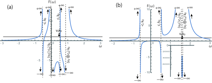
Figure 1: A plot of $F(\omega)$ in the relativistic cases of $c_{\rm i}\oplus c_{\rm e}\geq v_{0}$ with $v_{0}{\color[rgb]{0,0,0}=0.984c}=1$, $c_{\rm i}=c_{\rm e}{\color[rgb]{0,0,0}=0.984c}=1$ [panel (a), case (ii)] and of $c_{\rm i}\oplus c_{\rm e}<v_{0}$ with $v_{0}{\color[rgb]{0,0,0}=0.984c}=3$, $c_{\rm i}=c_{\rm e}{\color[rgb]{0,0,0}=0.328c}=1$ [panel (b), case (i)], where $\gamma_{0}^{3}=183.6$, that is, $\epsilon=1/10$ and $k=0.5313$. The cross point on the curve of $F(\omega)$ and the line $F=1$ give the dispersion relation. In the case of (a) $c_{\rm i}\oplus c_{\rm e}\geq v_{0}$ [case (ii)], all four solutions of the dispersion relation are real numbers. In the case of (b) $c_{\rm i}\oplus c_{\rm e}<v_{0}$ [case (i)], only two solutions of the dispersion relation are real numbers and two complex solutions exist. Not that in panel (b), $F$ between $\displaystyle\omega=(v_{0}\ominus c_{\rm e})k_{0}$ and $\omega=(v_{0}\oplus c_{\rm e})k_{0}$ is plotted in a separate box because its scale is quite different from the other range.

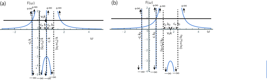
Figure 2: As Fig. 1, but for $F(\omega)$ in the non-relativistic cases of $c_{\rm i}+c_{\rm e}\geq v_{0}$ with $v_{0}=1$, $c_{\rm i}=c_{\rm e}=1$ [panel (a), case (ii)] and of $c_{\rm i}+c_{\rm e}<v_{0}$ with $v_{0}=3$, $c_{\rm i}=c_{\rm e}=1$ [panel (b), case (i)], where $\epsilon=1/1836$ ($\gamma_{0}=1$) and $k=0.5313$. In the non-relativistic case, we can simply write $c_{\rm i}\oplus c_{\rm e}=c_{\rm i}+c_{\rm e}$ and $c_{\rm i}\ominus c_{\rm e}=c_{\rm i}-c_{\rm e}$.

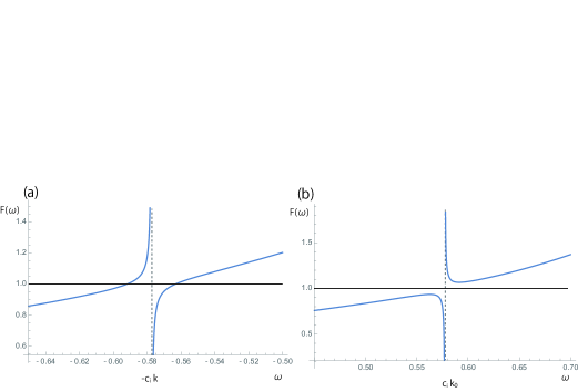
Figure 3: A zoomed-in version of the plot of $F(\omega)$ in the non-relativistic cases of $c_{\rm i}+c_{\rm e}\geq v_{0}$ with $v_{0}=1$, $c_{\rm i}=c_{\rm e}=1$ [case (ii)] around $\omega=-c_{\rm i}k=-0.577$ [panel (a)] and of $c_{\rm i}+c_{\rm e}<v_{0}$ with $v_{0}=3$, $c_{\rm i}=c_{\rm e}=1$ around $\omega=c_{\rm i}k=0.577$ [panel (b)], where $\epsilon=1/1836$ and $k=1/\sqrt{3}=0.577$.

$F(\omega)$ has four singular points, $\omega=\pm c_{\rm i}k$, $(v_{0}\ominus c_{\rm e})k$, $(v_{0}\oplus c_{\rm e})k$, where $\displaystyle v_{0}\ominus c_{\rm e}\equiv\frac{v_{0}-c_{\rm e}}{1-v_{0}v_{\rm e}/c^{2}}$. The behaviors of $F(\omega)$ at the singular points are as follows,

$$\lim_{\omega\rightarrow-c_{\rm i}k-0}F(\omega)=\infty, \lim_{\omega\rightarrow-c_{\rm i}k+0}F(\omega)=-\infty,$$ (25)

$$\lim_{\omega\rightarrow c_{\rm i}k-0}F(\omega)=-\infty, \lim_{\omega\rightarrow c_{\rm i}k+0}F(\omega)=\infty,$$ (26)

$$\lim_{\omega\rightarrow(v_{0}\ominus c_{\rm e})k-0}F(\omega)=\infty, \lim_{\omega\rightarrow(v_{0}\ominus c_{\rm e})k+0}F(\omega)=-\infty,$$ (27)

$$\lim_{\omega\rightarrow(v_{0}\oplus c_{\rm e})k-0}F(\omega)=-\infty, \lim_{\omega\rightarrow(v_{0}\oplus c_{\rm e})k+0}F(\omega)=\infty.$$ (28)

There are four kinds of patterns in the relationship of the four singular points: (i) $-c_{\rm i}k<c_{\rm i}k<(v_{0}\ominus c_{\rm e})k<(v_{0}\oplus c_{\rm e})k$, (ii) $-c_{\rm i}k<(v_{0}\ominus c_{\rm e})k\leq c_{\rm i}k<(v_{0}\oplus c_{\rm e})k$, (iii) $-c_{\rm i}k<(v_{0}\ominus c_{\rm e})k<(v_{0}\oplus c_{\rm e})k\leq c_{\rm i}k$, (iv) $(v_{0}\ominus c_{\rm e})k\leq-c_{\rm i}k<c_{\rm i}k<(v_{0}\oplus c_{\rm e})k$ (see Table 1). The topologies of the profiles of $F(\omega)$ in case (i) and case (ii) are drastically different and the numbers of real solutions for $F(\omega)=1$ are different. The profiles of $F(\omega)$ in the cases (ii), (iii), and (iv) are topologically identical and the numbers of the real solutions of $F(\omega)=1$ are the same. The condition for case (i) is given by (i) $c_{\rm i}<v_{0}\ominus c_{\rm e}$ and the condition of cases (ii), (iii), (iv) can be summarized as (ii–iv) $v_{0}\ominus c_{\rm e}\leq c_{\rm i}$ because $v_{0}$ is positive. The conditions for cases (i) and (ii–iv) are written as (i) $c_{\rm i}\oplus c_{\rm e}<v_{0}$ and (ii–iv) $v_{0}\leq c_{\rm i}\oplus c_{\rm e}$, respectively.

(i)	$-\infty$	$\cdots$	$-c_{\rm i}k$	$\cdots$	$c_{\rm i}k$	$\cdots$	$(v_{0}\ominus c_{\rm e})k$	$\cdots$	$(v_{0}\oplus c_{\rm e})k$	$\cdots$	$+\infty$
			–     +		–     +		–     +		–     +
$F(\omega)$	0	$\nearrow$	$+\infty$ $-\infty$	$\nearrow$ $\searrow$	$-\infty$ $+\infty$	$\searrow$ $\nearrow$	$+\infty$ $-\infty$	$\nearrow$ $\searrow$	$-\infty$ $+\infty$	$\searrow$	0
(ii)	$-\infty$	$\cdots$	$-c_{\rm i}k$	$\cdots$	$(v_{0}\ominus c_{\rm e})k$	$\cdots$	$c_{\rm i}k$	$\cdots$	$(v_{0}\oplus c_{\rm e})k$	$\cdots$	$+\infty$
(iii)	$-\infty$	$\cdots$	$-c_{\rm i}k$	$\cdots$	$(v_{0}\ominus c_{\rm e})k$	$\cdots$	$(v_{0}\oplus c_{\rm e})k$	$\cdots$	$c_{\rm i}k$	$\cdots$	$+\infty$
(iv)	$-\infty$	$\cdots$	$(v_{0}\ominus c_{\rm e})k$	$\cdots$	$-c_{\rm i}k$	$\cdots$	$c_{\rm i}k$	$\cdots$	$(v_{0}\oplus c_{\rm e})k$	$\cdots$	$+\infty$
$F(\omega)$	0	$\nearrow$	$+\infty$ $-\infty$	$\nearrow$	$+\infty$ $-\infty$	$\nearrow$ $\searrow$	$-\infty$ $+\infty$	$\searrow$	$-\infty$ $+\infty$	$\searrow$	0

Table 1: A plot of the singular points of $F(\omega)$. In the region of “$\nearrow$ $\searrow$”, $F(\omega)$ has its maximum value, and $F(\omega)$ in the region “$\searrow$ $\nearrow$” has its minimum value. “$\nearrow$” represents a monotonic increase and “$\searrow$” represents a monotonic decrease. In case (i), the number of the real number solutions of $F=1$ is two for a small enough wave number.

First, heuristically, we consider the relativistic case of $\gamma_{0}^{3}=183.6$, that is, $\epsilon=1/10$, because in the non-relativistic case of $\epsilon=1/1836$, the function $F(w)$ has a very fine structure that is difficult to understand. Hereafter, we treat $v_{0}$ and $\gamma_{0}$ as model-free parameters so that the light speed is $\displaystyle c=\frac{\gamma_{0}}{\sqrt{\gamma_{0}^{2}-1}}v_{0}\geq v_{0}$.

When $c_{\rm i}\oplus c_{\rm e}\geq v_{0}$ [case (ii)], the profile of $F(\omega)$ becomes as shown in Fig. 1 (a) for any $k$, where we set $\epsilon=1/10$, $c_{\rm i}=c_{\rm e}{\color[rgb]{0,0,0}=0.984c}=1$, $v_{0}{\color[rgb]{0,0,0}=0.984c}=1$ ($c=1.016$), and $k=0.5313$. Throughout this paper, for the numerical calculation, we normalize the velocity by $c_{\rm i}$. In the case of a normal plasma, the normalized value of the velocity is approximately the ion Mach number as long as $c_{\rm e}$ is not much larger than $c_{\rm i}$, because $c_{\rm i}$ is approximately the ion acoustic velocity $c_{\rm s}$. It is found that we always have four real solutions of $F(\omega)=1$, because there are four separate lines connecting the line $F=0$ ($F\longrightarrow 0$) and the region $F\longrightarrow\infty$. In the case of $c_{\rm i}\oplus c_{\rm e}\geq v_{0}$, the system is stable. This holds for any $\epsilon$ as shown in Fig. 2 (a) for the case of $\epsilon=1/1836$ ($\gamma_{0}=1,c\longrightarrow\infty$). We show the detail of the line of $F(\omega)$ around $\omega=-c_{\rm i}k$ in Fig. 3 (a), which clearly indicates two real solutions exist around $\omega=-c_{\rm i}k$. It is noted that the profiles of $F(\omega)$ in cases (ii), (iii), and (iv) are similar, and then the equation $F(\omega)=1$ has four real solutions, not only in case (ii) but also in cases (iii) and (iv).

On the other hand, in the case of $c_{\rm i}\oplus c_{\rm e}<v_{0}$ [case (i)], the topological profile of $F(\omega)$ changes drastically. We plot $F(\omega)$ in the case of $\epsilon=1/10$ ($\gamma_{0}^{3}=183.6$), $c_{\rm i}=c_{\rm e}{\color[rgb]{0,0,0}=0.328c}=1$, and $v_{0}{\color[rgb]{0,0,0}=0.984c}=3$ ($c=3.048$) with

$$k=k_{0}(v_{0},c_{\rm i},c_{\rm e})\equiv\frac{1}{\sqrt{(c_{\rm i}-v_{0})^{2}-c_{\rm e}^{2}(1-v_{0}c_{\rm i}/c^{2})^{2}}}=\frac{\omega_{\rm pe}}{\sqrt{(c_{\rm i}-v_{0})^{2}-c_{\rm e}^{2}(1-v_{0}c_{\rm i}/c^{2})^{2}}},$$ (29)

in Fig. 1 (b). Here, on the right-hand side of Eq. (29), the unit of time is recovered from the specified unit of time $\omega_{\rm pe}^{-1}$. It is found that $F(\omega)=1$ has only two real solutions because there are only two separate lines connecting the line $F=0$ ($F\longrightarrow 0$) and the region $F\longrightarrow\infty$, and the other lines never touch or cross the line $F=1$. The other two solutions are complex, which indicates that the two fluids are unstable. This instability is recognized as the “two-stream instability”.Chen (2016)

In the non-relativistic case of $\epsilon=1/1836$ ($\gamma_{0}=1$, $c\longrightarrow\infty$), $c_{\rm i}=1$, $c_{\rm e}=1$, $v_{0}=3$ with $k=k_{0}(v_{0},c_{\rm i},c_{\rm e})$, we plot the curve of $F(\omega)$ in Fig. 2 (b). $F(\omega)=1$ has only two real solutions. This is because the curve $F(\omega)$ never passes $\omega=c_{\rm i}k$, as shown in Fig. 3 (b). The other two solutions are complex, which indicates that the two-fluid system is unstable. We then obtain the criterion of the two-stream instability, $c_{\rm i}+c_{\rm e}=c_{\rm i}\oplus c_{\rm e}<v_{0}$ for any positive $\epsilon$, in the non-relativistic case. In summary, the criterion of the two-stream instability is given by Eq. (24) in the special relativistic framework.

To investigate the range of the wave number of the unstable mode in case (i), we write $F(\omega)$ with $k=k_{0}$ as $F_{0}(\omega)$. We call the maximum value of $F_{0}(\omega)$ in the region $-c_{\rm i}k<\omega<c_{\rm i}k$ $F_{\rm 0,i}^{\rm max}$ and the minimum value of $F_{0}(\omega)$ in the region $c_{\rm i}k<\omega<(v_{0}\oplus c_{\rm e})k$ $F_{\rm 0,b}^{\rm min}$. The wave number of the unstable mode is given by $k_{0}\sqrt{\max(0,F_{\rm 0,i}^{\rm max})}<k<k_{0}\sqrt{F_{\rm 0,b}^{\rm min}}$. When we consider the imaginary case with $\epsilon=1$ corresponding a non-relativistic pair plasma (an electron-positron plasma), the mode of $0<k<k_{0}$ is unstable because $F_{\rm 0,i}^{\rm max}<0$ and $F_{\rm 0,b}^{\rm min}>1$. On the other hand, in the non-relativistic realistic case of a normal plasma ($\epsilon=1/1836\ll 1$), the unstable mode is restricted to $k\approx k_{0}$ because $F_{\rm 0,i}^{\rm max}\approx F_{\rm 0,b}^{\rm min}$.

It is noteworthy that in the non-relativistic case of $\epsilon=1/1836$, $c_{\rm i}=1$, $c_{\rm e}=1$, $v_{0}=3$ ($\gamma_{0}=1$, $c\longrightarrow\infty$), we find the curve of $F(\omega)$ with $k\geq 1.04k_{0}$ or $k\leq 0.96k_{0}$ crosses the line $F=1$ around $\omega\sim c_{\rm i}k$, while the curve of $F(\omega)$ with $k\leq 1.03k_{0}$ and $k\geq 0.97k_{0}$ never crosses the line $F=1$ around $\omega\sim c_{\rm i}k$. Then, the equation $F(\omega)=1$ has four real solutions and we find that the mode with with $k\geq 1.04k_{0}$ or $k\leq 0.96k_{0}$ is stable, while the mode with with $k\leq 1.03k_{0}$ and $k\geq 0.97k_{0}$ is unstable. Eventually, we conclude that, in the case of a normal plasma ($\epsilon=1/1836\ll 1$), the wave number of the unstable mode can be fixed to approximately $k\cong k_{0}(v_{0},c_{\rm i},c_{\rm e})$. In such a case, the difference between the complex solution of $F(\omega)=1$ and $\omega=b$ is infinitesimally small and we obtain the approximate solution of $\omega=b+ip$, where $\displaystyle p=\pm\frac{1}{2k_{0}}\sqrt{\frac{\epsilon}{c_{\rm i}(v_{0}-c_{\rm e})}}$. We then find the growth rate of the two-stream instability

$$p_{\rm gr}=\frac{1}{2}\sqrt{\epsilon\frac{(v_{0}-c_{\rm i})^{2}-c_{\rm e}^{2}}{c_{\rm i}(v_{0}-c_{\rm e})}}\omega_{\rm pe}$$ (30)

in the non-relativistic case, where we recover the dimension of time.

This linear analysis yields the criterion of the two-stream instability in Eq. (24). In an extremely low-density plasma, the current may become unstable due to the two-stream instability. This instability may be important for the plasma supply mechanism of relativistic jets from AGNs, as shown in the next section.

III Discussion

In this study, we have presented a simple criterion for the two-stream instability within the relativistic framework: the instability arises if and only if $c_{\rm i}\oplus c_{\rm e}<v_{0}$. This criterion is derived from the two-fluid equations for a plasma with a finite temperature. The two-stream instability with this criterion is identical to the Buneman instability because the electron drift velocity is large compared to the plasma thermal velocity.

It is worth noting that Eq. (24) can be written as follows in order to determine the relativistic effect on the two-stream instability criterion:

$$\frac{\gamma_{\rm i}\gamma_{\rm e}}{\gamma_{\rm 0}}(c_{\rm i}+c_{\rm e})<v_{0},$$ (31)

where $\gamma_{\rm i}=(1-c_{\rm i}^{2}/c^{2})^{-1/2}$ and $\gamma_{\rm e}=(1-c_{\rm e}^{2}/c^{2})^{-1/2}$ are the Lorentz factors of the sound velocities in the ion and electron fluids. Equation (31) clearly indicates that the thermal relativistic effect suppresses the instability, while the relativistic effect of the electron drift motion enhances the instability.

This simple criterion for the instability described by Eq. (31) applies to the plasma source region of a relativistic jet close to a spinning supermassive black hole, such as the active galactic nucleus (AGN) of the elliptical giant galaxy M87. In some regions of the universe, such as at the pole of a black hole of an AGN like M87, McKinney (2009); Event Horizon Telescope Collaboration (2019); Porth et al. (2019) it is anticipated that plasmas with very low densities and strong magnetic fields exist. Here, a strong magnetic field indicates that the magnetic field energy is greater than the rest mass energy density of the plasma. A number of numerical simulations of general relativistic magnetohydrodynamics with zero electric resistivity (ideal GRMHD) imply the presence of a very strong magnetic field in a foot-point region of the relativistic jet, and the magnetic field lines along the relativistic jet are anchored to the horizon of the black hole. Near the horizon, the plasma in the magnetic flux tube anchored to the horizon falls into the black hole. Because the magnetic field flux is supplied by an accretion disk and the magnetic field in an accretion disk is turbulent, a large antiparallel magnetic field is predicted to exist in the foot-point region of the jet. At the boundary of the jet and the inflow toward the black hole, the plasma density decreases infinitesimally because magnetic surfaces disturb the plasma supply from outside the region to the jet as a result of its frozen-in state. If the plasma density decreases sufficiently, the drift velocity of the electron fluid increases in the current sheet, sustaining the antiparallel magnetic field. In such a scenario, the drift velocity of the electron fluid exceeds the threshold of the two-stream instability, causing the instability to disrupt the current sheet and annihilate the magnetic field in the jet foot-point region. The annihilation of the magnetic field in this region causes the plasma from outside the region to rush in and supply the plasma to the jet. This is the first mechanism proposed to explain a normal plasma supply to the relativistic jet ejected from an AGN, whereas a variety of pair plasma supply mechanisms have previously been described in the strong magnetic field region close to spinning supermassive black holes. Blandford & Znajek (1977); Levinson (2018); Toma (2020) Here, we have demonstrated that the two-stream instability in a plasma of extremely low density could transport the normal plasma and magnetic field of the disk to the plasma source region of the jet. Once the plasma and magnetic field are supplied to the jet-forming region, the mechanism seen in ideal GRMHD simulations Gammie et al. (2003); Mizuno et al. (2004); Koide et al. (2006); Nagataki (2009); McKinney (2006, 2009); Porth et al. (2019); Event Horizon Telescope Collaboration (2019); EHT Collaboration (2022) and the general relativistic analytical theories of steady outflow Takahashi (1990); Hirotani (1992) can work to produce a relativistic jet composed of normal plasma. On the contrary, for the elemental process due to the two-stream instability, we can use the special relativistic criterion even for plasma near the supermassive black hole, because the two-stream instability is a local phenomenon and we can neglect the tidal force since the characteristic length of the instability $l_{\rm c}$ is less than $2\pi f_{\rm c}\lambda_{\rm D}$ from Eq. (29) and $\lambda_{\rm D}$ is much smaller than the gravitational radius of the supermassive black hole $r_{\rm H}$. Here, $\lambda_{\rm D}$ is the Debye length $\displaystyle\lambda_{\rm D}\equiv\frac{c_{\rm e}}{\omega_{pe}}$ and $f_{\rm c}$ is defined by $v_{0}\ominus c_{\rm i}=f_{\rm c}c_{\rm e}$, where $f_{\rm c}$ is greater than unity but not much greater. We can then choose local inertial frame coordinates such that no gravitational field appears according to the equivalence principle.

Let us now consider the criterion of the current disruption in the low-density region at the pole of the black hole in an AGN, for example, at the center of M87. We assume an equilibrium condition with respect to the current sheet between the antiparallel magnetic fields and the pressure of the normal plasma (Fig. 4),

$$p_{0} =\frac{B_{0}^{2}}{2\mu_{0}}, \mu_{0}J\delta =2B_{0}, J =ne\gamma_{0}v_{0}=en_{0}v_{0},$$ (32)

$$p_{0} =P_{+}+P_{-}, P_{+} =n_{+}T_{+}=n_{0}T, P_{-} =n_{-}T_{-}=\frac{\xi}{\gamma_{0}}n_{0}T,$$ (33)

where $\delta$ is the width of the current sheet.

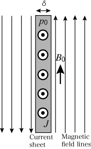
Figure 4: A schematic picture of the current sheet in the antiparallel magnetic field.

Here, we assume the pressure outside of the current sheet is negligibly small. The magnetic field outside of the current sheet is denoted $B$, and the particle number density, total pressure, ion pressure, electron pressure, current density, ion temperature, and electron temperature in the current sheet are denoted $n_{0}$, $p_{0}$, $P_{+}$, $P_{-}$, $J$, $T_{+}=T$, $T_{-}=\xi T$ ($\xi$ is a constant parameter). Using Eqs. (32)–(33), we have

$$P_{+} =\frac{\gamma_{0}}{\xi+\gamma_{0}}\frac{B_{0}^{2}}{2\mu_{0}},P_{-}=\frac{\xi}{\xi+\gamma_{0}}\frac{B_{0}^{2}}{2\mu_{0}},$$ (34)

$$v_{0} =\frac{2B_{0}}{\mu_{0}en_{0}\delta}=2\sqrt{\frac{m\sigma c^{2}}{\mu_{0}e^{2}n_{0}\delta^{2}}},\gamma_{0}=\left(1-\frac{4m\sigma}{\mu_{0}e^{2}n_{0}\delta^{2}}\right)^{-1/2},$$ (35)

where $\sigma$ is the magnetization parameter defined by $\displaystyle\sigma=\frac{B_{0}^{2}}{mn_{0}c^{2}}$ with $m=m_{+}+m_{-}$. Equations (31) and (34) – (35) yield the instability criterion of the two-stream instability in the current sheet

$$n_{0}\delta^{2} <\frac{8m_{\rm e}}{\mu_{0}e^{2}}\frac{1+\xi/\gamma_{0}}{(\gamma_{\rm i}\gamma_{\rm e})^{2}}\frac{1}{f^{2}}+\frac{4m}{\mu_{0}e^{2}}\sigma=2.24\times 10^{14}{\rm[m^{-1}]}\left[\frac{1+\xi/\gamma_{0}}{(\gamma_{\rm i}\gamma_{\rm e})^{2}}\frac{1}{f^{2}}+\frac{m}{2m_{\rm e}}\sigma\right],$$ (36)

where we define $\displaystyle f\equiv\sqrt{\frac{\xi\Gamma_{-}}{\bar{M}_{-}/m_{\rm e}}}+\sqrt{\frac{\Gamma_{+}}{\bar{M}_{+}/m_{\rm e}}}$, $\displaystyle\bar{M}_{+}\equiv m_{+}+\frac{\Gamma_{+}}{\Gamma_{+}-1}\frac{m}{2(1+\xi/\gamma_{0})}\sigma$, $\displaystyle\bar{M}_{-}\equiv m_{-}+\frac{\Gamma_{-}}{\Gamma_{-}-1}\frac{\xi m}{2(1+\xi/\gamma_{0})}\sigma$.

In the case of the non-relativistic magnetic field limit, $\displaystyle\sigma\ll\frac{m_{\rm e}}{m_{+}}\ll 1$ and $\displaystyle\Gamma_{-}=\frac{5}{3}$, we have

$$n_{0}\delta^{2}<1.34\times 10^{14}\left(1+\frac{1}{\xi}\right)\;{\rm m^{-1}}.$$ (37)

In the case of a relativistic magnetic field, $\sigma\gg 1$, $\gamma_{0}\gg 1$, and $\displaystyle\Gamma_{\pm}=\frac{4}{3}$, we obtain

$$n_{0}\delta^{2}<5.59\times 10^{17}\sigma\;{\rm m^{-1}}.$$ (38)

Comparing Eqs. (37) and (38), we find that the critical value of $n_{0}\delta^{2}$ in the case of the relativistically strong magnetic field is more than $1\,000$ times larger than that in the case of a non-relativistic magnetic field. This clearly demonstrates that special relativistic effects drastically enhance the two-stream instability.

Using the parameters of the disk observed for Sgr A* by EHT (EHT Collaboration, 2022): $n_{0}=10^{12}\,\rm m^{-3}$, $\xi=1$, $\gamma_{0}=\gamma_{\rm i}=\gamma_{\rm e}=1$, we obtain the stable condition to be $\delta>10\,$m from Eq. (37) and the threshold length of the instability to be $l_{\rm th}^{\rm SgrA*}=10\,$m. With respect to the AGN of M87 (M87*), using the parameters of EHTEvent Horizon Telescope Collaboration (2019) — $n_{0}=3\times 10^{10}\,\rm m^{-3}$, $\xi=1$, and $\gamma_{0}=\gamma_{\rm i}=\gamma_{\rm e}=1$ — the threshold length of the instability is given as $l_{\rm th}^{\rm M87*}=100\,$m from Eq. (37). Because the scales of the turbulence in the accretion disks surrounding the black hole in Sgr A* and M87* are of the order of $\delta_{\rm SgrA*}=10^{10}\,$ m and $\delta_{\rm M87*}=7\times 10^{13}\,$ m, respectively, and the disks are free of the two-stream instability, these conditions appear to be reasonable: $\delta_{\rm SgrA*}\gg l_{\rm th}^{\rm SgrA*}$ and $\delta_{\rm M87*}\gg l_{\rm th}^{\rm M87*}$. In the very low-density region, like the region at the footpoint of an AGN jet, the two-stream instability is caused when the density becomes small enough, for example, if we consider the thickness of the current sheet to be $\delta=5.6\times 10^{5}\,$ m and $\sigma=10$, the threshold density of the instability is given by $n_{\rm th}=10^{4}\,\rm m^{-3}$ from Eq. (38). When the density falls below this threshold, the two-stream instability occurs in the current sheet with a large current density between the strong antiparallel magnetic field regions to disrupt the current sheet, and magnetic field annihilation occurs. This magnetic field annihilation should trigger the supply of plasma from outside of the region to the low-density region. This mechanism of plasma supply may work in the strong magnetic field region near the black hole to form the relativistic jet in the AGN of M87. On the other hand, no relativistic jet is observed in Sgr A*, while a strong magnetic field region is expected to exist near the black hole in the AGN of Sgr A*.EHT Collaboration (2022) The difference between the AGNs of M87 and Sgr A* may come from the direction of the strong magnetic field. That is, in the strong magnetic field region of the AGN in Sgr A*, the magnetic field lines are aligned in the same poloidal direction and no antiparallel magnetic field is formed. In such a strong magnetic field region, a current sheet is not formed because of the lack of an antiparallel magnetic field, and the two-stream instability is never triggered. An accurate observation of the circular polarization of the radio wave would be helpful to verify this model of the plasma supply mechanism in the relativistic jet-forming regions of AGNs.

Due to the magnetorotational instability, the magnetic field in an accretion disk is observed to be turbulent. A strong magnetic field around a spinning black hole is formed from the magnetic field in a disk. It appears that an antiparallel magnetic field would arise in an area with a strong magnetic field. In the near future, numerical simulations beyond ideal GRMHD should be used to clarify the details of the entire process of jet formation, including the formation and annihilation of the antiparallel magnetic field. Such numerical simulations are also expected to reveal the difference between the magnetic field configurations in strong magnetic field regions with and without relativistic jets around the black holes in M87* and Sgr A*. During the two-stream instability process in a realistic situation, the plasma would be non-uniform and magnetized. The dependence of the instability on these additional factors is important and will be clarified using the relativistic two-fluid equations including these factors in the near future.