Mitigating Exploitation Bias in Learning to Rank with an Uncertainty-aware Empirical Bayes Approach

Abstract.

Ranking is at the core of many artificial intelligence (AI) applications, including search engines, recommender systems, etc. Modern ranking systems are often constructed with learning-to-rank (LTR) models built from user behavior signals. While previous studies have demonstrated the effectiveness of using user behavior signals (e.g., clicks) as both features and labels of LTR algorithms, we argue that existing LTR algorithms that indiscriminately treat behavior and non-behavior signals in input features could lead to suboptimal performance in practice. Particularly because user behavior signals often have strong correlations with the ranking objective and can only be collected on items that have already been shown to users, directly using behavior signals in LTR could create an exploitation bias that hurts the system performance in the long run.

To address the exploitation bias, we propose EBRank, an empirical Bayes-based uncertainty-aware ranking algorithm. Specifically, to overcome exploitation bias brought by behavior features in ranking models, EBRank uses a sole non-behavior feature based prior model to get a prior estimation of relevance. In the dynamic training and serving of ranking systems, EBRank uses the observed user behaviors to update posterior relevance estimation instead of concatenating behaviors as features in ranking models. Besides, EBRank additionally applies an uncertainty-aware exploration strategy to explore actively, collect user behaviors for empirical Bayesian modeling and improve ranking performance. Experiments on three public datasets show that EBRank is effective, practical and significantly outperforms state-of-the-art ranking algorithms.

1. Introduction

Ranking techniques have been extensively studied and used in modern Information Retrieval (IR) systems such as search engines, recommender systems, etc. Among different ranking techniques, learning to rank (LTR), which relies on building machine learning (ML) models to rank items, is one of the most popular ranking frameworks (Liu et al., 2009). In particular, industrial LTR systems are usually constructed with user behavior feedback/signals since user behaviors (e.g., click, purchase) are cheap to get and direct indicate results’ relevance from the user’s perspective (Wang et al., 2016). For example, previous studies  (Wang et al., 2016; Joachims et al., 2017; Ai et al., 2018b) have shown that, instead of using expensive relevance annotations from experts, effective LTR models can be learned directly from training labels constructed with user clicks. Besides using clicks as training labels, many industrial IR systems have also considered features extracted from user clicks (called behaviour features in  (Yang et al., 2022) or click-through features in (Gao et al., 2009)) for their LTR models. For example, ranking features extracted from clicks are used in search engines like Yahoo and Bing (Chapelle and Chang, 2011; Qin et al., 2010). Agichtein et al. (2006) has shown that, by incorporating user clicks as behavior features in ranking systems, the performance of competitive web search ranking algorithms can be improved by as much as 31% relative to the original performance.

However, without proper treatment, LTR with user behaviors can also damage ranking quality in the long term (Yang et al., 2022; Li et al., 2020; Kveton et al., 2022). Specifically, user behavior signals usually have high correlations with the training labels, no matter whether the labels are constructed from expert annotations or from users’ behavior. Such high correlation can easily make input features built from user behavior signals, referred to as the behavior features, overwhelm other features in training, dominate model outputs, and be over-exploited in inference. Such an over-exploitation phenomenon would hurt practical ranking systems when user behavior signals are unevenly collected on different candidate items (Gupta et al., 2020; Li et al., 2020). For example, we can only collect user clicks on items already presented to users. Items that lack historical click data, including new items that have not yet been presented to users, would be at a disadvantage in ranking. The disadvantage, referred to as the exploitation bias (Yang et al., 2022), can be more severe when we use user clicks/behaviors as both labels and features, which is a common practice in real-world LTR systems (Yang et al., 2022; Gupta et al., 2020; Chapelle and Chang, 2011; Qin et al., 2010; Gao et al., 2009). One similar concept is selection bias (Oosterhuis and de Rijke, 2020). However, selection bias usually refers to the bias that occurs when user clicks are used as training labels. In contrast, exploitation bias goes one step further and considers the bias that arises in a more realistic scenario where user behavior is both the training labels and features.

In this paper, we solve the above exploitation bias with an uncertainty-aware empirical Bayesian based algorithm, EBRank. Specifically, we consider a general application scenario where a ranking system is built with user behavior signals (e.g. clicks) in both its input and objective function. We show that, without differentiating the treatment of behavior signals and non-behavior signals in input features, existing LTR algorithms could suffer severely from exploitation bias. By differentiating behavior signals and non-behavior signals, the proposed algorithm, EBRank, uses a sole non-behavior feature based prior model to give a prior relevance estimation. With more behavior data collected from the online serving process of the ranking system, EBRank gradually updates its posterior relevance estimation to give a more accurate relevance estimation. Besides the empirical Bayesian model, we also proposed a theoretically principled exploration algorithm that joins the optimization of ranking performance with the minimization of model uncertainty. Experiments on three public datasets show that our proposed algorithm can effectively overcome exploitation bias and deliver superior ranking performance compared to state-of-the-art ranking algorithms. To summarize, our contributions are

• We demonstrate that existing LTR algorithms suffer severely from exploitation bias.

• We propose EBRank, a Bayesian-based LTR algorithm that mitigates exploitation bias.

• We propose an uncertainty-aware exploration strategy for EBRank that optimizes ranking performance while minimizing model uncertainty.

2. Related Work

In general, there are three lines of research that directly relate to this paper: behavior features in LTR, unbiased/online learning to rank, and uncertainty in ranking.

Ranking exploitation with behavior features. As an important relevance indicator, user behavior signals have been important components for constructing modern IR systems (Qin et al., 2010). (Agichtein et al., 2006; Macdonald et al., 2012) showed that incorporating user behavior data as features can significantly improve the ranking performance of top results. However, incorporating behavior features without proper treatments could hurt the effectiveness of LTR systems by amplifying the problem of over-exploitation and over-fitting, i.e., exploitation bias (Yang et al., 2022). Oosterhuis and de Rijke (2021b); Li et al. (2020); Kveton et al. (2022) discussed the generation problems and cold-start problems when using behavior signals. Some strategies were proposed to overcome the exploitation bias by predicting behavior features with non-behavior features (Gupta et al., 2020; Han et al., 2022) or by actively collecting user behavior for new items (Yang et al., 2022; Li et al., 2020) via exploration.

Unbiased/Online Learning to Rank. Using biased and noisy user clicks as training labels for LTR has been extensively studied in the last decades (Tran et al., 2021; Ai et al., 2021; Ovaisi et al., 2020). Among different unbiased LTR methods, online LTR chooses to actively remove the bias with intervention based on bandit learning (Wang et al., 2019; Zoghi et al., 2017) or stochastic ranking sampling (Oosterhuis and de Rijke, 2018). While offline LTR methods usually train LTR models with offline click logs based on techniques such as counterfactual learning (Joachims et al., 2017; Ai et al., 2018a; Yang et al., 2020; Agarwal et al., 2019a). Existing unbiased LTR methods effectively remove bias when clicks are treated as labels. In this work, we investigate and show that existing unbiased LTR methods mostly suffer the exploitation bias brought by introducing clicks as features.

Uncertainty in ranking. One of the first studies of uncertainty in IR is Zhu et al. (2009), where the variance of a probabilistic language model was treated as a risk-based factor to improve retrieval performance. Recently, uncertainty estimation techniques for deep learning models have also been introduced into the studies of neural IR models (Cohen et al., 2021; Penha and Hauff, 2021; Wang et al., 2021). Uncertainty quantification is an important IR community for many downstream tasks. For example, (Yang et al., 2022; Jeunen and Goethals, 2021; Liang and Vlassis, 2022; Cief et al., 2022) proposed uncertainty-aware exploration ranking algorithms. Instead of optimizing ranking performance directly, existing studies have shown that uncertainty can help improve query performance prediction (Roitman et al., 2017), query cutoff prediction (Lien et al., 2019; Culpepper et al., 2016), and ranking fairness (Yang et al., 2023).

3. Background

In this section, we introduce some preliminary knowledge of this work, including the workflow of ranking services, modeling of users’ behavior and utilities to evaluate a ranking system.

Table 1. A summary of notations.

$d,q,D(q)$	For a query $q$, $D(q)$ is the set of candidates items. $d\in D(q)$ is an item.
$e,r,c$	All are binary random variables indicating whether an item $d$ is examined ($e=1$), is relevant ($r=1$) and clicked ($c=1$) by a user respectively.
$R$,$p$,$E,\pi$,$n$	$R=P(r=1)$, is the probability an item $d$ perceived as relevant. $p=P(e=1)$ is the examination probability. $\pi$ is a ranklist. $E$ is an item’s accumulated examination probability. $n$ is the number of times item $d$ has been presented to users (see Eq.9).
$k_{s},k_{c}$	Users will stop examining items lower than rank $k_{s}$ due to selection bias (see Eq. 3). $k_{c}$ is the cutoff prefix to evaluate Cum-NDCG and $k_{c}\leq k_{s}$.
$x^{b},x^{nb}$	$x^{b}$ denotes ranking features derived from user feedback behavior, while $x^{nb}$ denotes ranking features derived from non-behavior features.

The Workflow of Ranking Services.

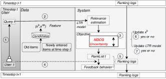
Figure 1. Workflow of ranking services.

In Figure 1, we use web search as an example to introduce the workflow of ranking service in detail, but the method we propose in this paper can also be extended to the recommendation or other ranking scenarios. At time step $t$, a user issues a query $q_{t}$. Corresponding to this query, there exist candidate items which include old items and new items introduced at time step $t$. These items are represented as features, which include behavior signals $x^{b}$ and non-behavior features $x^{nb}$ (a detailed discussion about features is given in the following paragraph). Based on the features, an LTR model will predict the relevance of each candidate item, and the ranking optimization methods will generate the ranked list by optimizing some ranking objectives. Different ranking objectives can be adopted here, such as maximizing NDCG (see Eq. 6) while minimizing the uncertainty in relevance estimation. After examining the ranked list, the user will provide behavior feedback, such as clicks. The rank list and user feedback behavior will be appended to the ranking logs. We need to decide whether to update the LTR model and behavior features or not. In practice, such updates are usually conducted periodically since real-time updating ranking systems are often not preferable.

Features. In this paper, LTR features are categorized into two groups based on Qin et al. (2010). The first group is non-behavior features, denoted as $x^{nb}$, which show items’ quality and the degree of matching between item and query. Example $x^{nb}$ can be BM25, query length, tf-idf, features from pre-trained (large) language models, etc. Non-behavior features $x^{nb}$ are usually stable and static. The second group is behavior features, denoted as $x^{b}$, which are usually derived from user behavior data, which can be click-through-rate, dwelling time, click, etc. $x^{b}$ are direct and strong indicators of relevance from the user’s perspective since $x^{b}$ are collected directly from the user themselves. Unlike $x^{nb}$, $x^{b}$ are dynamically changing and constantly updated. In this paper, we only focus on one type of user behavior data, i.e., clicks. Extending our work to other types of user behaviors is also straightforward, and we leave them for future studies.

Partial and Biased User Behavior. Although user behavior is commonly used in LTR, user behavior is usually biased and partial. Specifically, a user will provide meaningful feedback click ($c=1$) only when a user examines ($e=1$) the item, i.e.,

(1) $$\vspace{-2pt}c=\begin{cases}r,&\text{if}\quad e=1\\ 0,&\text{otherwise}\end{cases}\vspace{-2pt}$$

where $r$ indicates if a user would find an item $d$ as relevant. Here $c,r,e$ are random binary variables. A detailed summary of notations is in Table 1. Following (Ai et al., 2018b; Wang et al., 2016), we model users’ click behavior as follows,

(2) $$\vspace{-2pt}P(c=1)=P(r=1)P(e=1)\vspace{-2pt}$$

For different items, the examination probability $P(e=1)$ are usually different. In this paper, we model examination differences with the two most important biases, i.e., positional bias and selection bias. The position bias (Craswell et al., 2008) assumes the examination probability of an item $d$ solely relies on the rank (position) within a ranklist $\pi$ and we model it with $P(e=1|d,\pi)=p_{rank(d|\pi)}$ to simplify notation. The selection bias (Oosterhuis and de Rijke, 2021a, 2020) exists when not all of the items are selected to be shown to users, or some lists are so long that no user will examine the entire lists. The selection bias is modeled as,

(3) $$\vspace{-2pt}p_{rank(d|\pi)}=0\quad\text{if}\quad rank(d|\pi)>k_{s}\vspace{-2pt}$$

where $k_{s}$ is the lowest rank that will be examined.

Exploitation Bias.

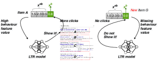
Figure 2. Toy example to show the exploitation bias. Old item A and new item G have the same non-behavior ($x^{nb}$) features, while item G’s behavior features ($x^{b}$) is 0 as it has not been shown to users before. Item G will be discriminated against if the LTR model over-exploits and heavily relies on $x^{b}$.

In Figure 2, we give a toy example to illustrate the exploitation bias. The exploitation bias usually happens because behavior features in LTR models will overwhelm other features since behavior features are strong indicators of relevance and highly correlated with training labels. In this example in Figure 2, due to the overwhelming importance of behavior features, newly introduced item G will be discriminated by the LTR model and ranked low when its user behavior information is missing.

Ranking utility. In this paper, ranking utility is evaluated by measuring a ranking system’s ability to put relevant items on top ranks effectively. Firstly, the relevance for a $(d,q)$ pair is

(4) $$R(d,q)=p(r=1|d,q)$$

is defined as the probability of an item $d$ being considered relevant to a given query $q$. One widely-used ranking utility measurement is DCG (Järvelin and Kekäläinen, 2002). For a ranked list $\pi$ corresponding to a query $q$, we define $\textit{DCG}@k_{c}$ as

(5) $$\vspace{-2pt}\textit{DCG}@k_{c}(\pi)=\sum_{i=1}^{k_{c}}R(\pi[i],q)\lambda_{i}=\sum_{i=1}^{k_{c}}R(\pi[i],q)\cdot p_{i}\vspace{-2pt}$$

where $\pi[i]$ indicates the $i^{th}$ ranked item in the ranked list $\pi$; $R(\pi[i],q)$ indicates item $\pi[i]$’s relevance to query $q$; $\lambda_{i}$ indicates the weight we put on $i^{th}$ rank; cutoff $k_{c}$ indicates the top $k_{c}$ ranks we evaluate. In this paper, when cutoff $k_{c}$ is not specified, there is no cutoff. $\lambda_{i}$ usually decreases as rank $i$ increases since top ranks are generally more important. For example, $\lambda_{i}$ is sometimes set to $\frac{1}{\log_{2}(i+1)}$. In this paper, we follow (Singh and Joachims, 2018) to choose the $i^{th}$ rank’s examining probability $p_{i}$ as $\lambda_{i}$. Then, we can get normalized-DCG ($\textit{NDCG}\in[0,1]$) by normalizing $\textit{DCG}@k_{c}(\pi)$,

(6) $$\vspace{-2pt}\textit{NDCG}@k_{c}(\pi)=\frac{\textit{DCG}@k_{c}(\pi)}{\textit{DCG}@k_{c}(\pi^{*})}\vspace{-2pt}$$

where $\pi^{*}$ is the ideal ranked list constructed by arranging items according to their true relevance. Furthermore, we could define discounted Cumulative NDCG (Cum-NDCG) as ranking effectiveness,

(7) $$\vspace{-2pt}\begin{split}\textit{Cum-NDCG}@k_{c}=\sum_{\tau=1}^{t}\gamma^{t-\tau}\textit{NDCG}@k_{c}(\pi_{\tau})\end{split}\vspace{-2pt}$$

where $0\leq\gamma\leq 1$ is the discounted factor, $t$ is the current time step. Note that $\gamma$ is a constant number for evaluating ranking performance (Wang et al., 2018b). Compared to NDCG, Cum-NDCG can better evaluate ranking effectiveness for online ranking services  (Schuth et al., 2013).

Uncertainty in relevance estimation. In real-world applications, the true relevance $R$ is usually unavailable. Relevance estimation, denoted as $\hat{R}$, is usually needed for ranking optimization. However, $\hat{R}$ usually contains uncertainty (variance), denoted as $\textit{Var}[\hat{R}]$. Furthermore, we introduce the query-level uncertainty in relevance estimation,

(8) $$\vspace{-2pt}U(q)=\sum_{d\in D(q)}\textit{Var}[\hat{R}(d,q)]\vspace{-2pt}$$

which will be used to guide ranking exploration. We leave more advanced query-level uncertainty formulations for future study.

4. Proposed Method

In this section, we propose an uncertainty-aware Empirical Bayes (EB) based learning to rank algorithm, EBRank, which can effectively overcome exploitation bias. We formally introduce the proposed algorithm EBRank In Sec .4.1. And we dive into the theoretical derivation of EBRank, which includes ranking objectives, Empirical Bayes modeling, and uncertainty reduction in Sec. 4.2, 4.3 and 4.4, repectively.

4.1. The proposed algorithm: EBRank

In this section, we give a big picture of the proposed Empirical Bayesian Ranking (EBRank) in Algorithm 1. Prior to serving users, we initialize a list, $\mathcal{H}$, to store ranking logs. At each time step, we append four elements, $[u_{t},q_{t},\pi_{t},c_{t}]$, to $\mathcal{H}$. Here, $u_{t},q_{t},\pi_{t},c_{t}$ are the user, the query, the presented ranklist, and the user clicks at time step $t$. If initial ranking logs exist prior to using EBRank, we will also append them to $\mathcal{H}$. Besides ranking logs, we initialize a model $f_{\theta}$, referred to as the prior model, parameterized by $\theta$, which takes non-behavior features as input. $f_{\theta}$ can be any trainable parameterized model, such as a neural network, tree-based model and etc. When EBRank begins to serve users ($t>0$), new candidates will be constantly appended to each query’s candidates set, $D(q_{t})$. Then $\forall d\in D(q_{t})$, we construct an auxiliary list $\mathcal{A}(d,q_{t})=[\alpha,\beta,n,C,E]$, where

(9) $$\begin{split}[\alpha,\beta]&=f_{\theta}\big{(}x^{nb}(d,q_{t})\big{)}\\ n&=\sum_{\tau\in T(t,d,q_{t})}1\\ C&=\sum_{\tau\in T(t,d,q_{t})}\frac{c(d|\pi_{\tau})}{p_{rank(d|\pi_{\tau})}}\\ E&=\sum_{\tau\in T(t,d,q_{t})}p_{rank(d|\pi_{\tau})}\\ T(t,d,q_{t})=\bigg{[}\tau\quad\text{if}\quad\mathbb{I}&(d\in\pi_{\tau})\mathbb{I}(q_{\tau}=q_{t})\quad\text{for}\quad 0\leq\tau<t\bigg{]}\end{split}$$

where the prior model $f_{\theta}$ takes the non-behavior feature $x^{nb}$ as input and exports two numbers, i.e., $[\alpha,\beta]$. $T(t,d,q_{t})$ is a subset of historical time steps when item $d$ is presented in query $q_{t}$’s ranklists in the past and $\mathbb{I}$ is the indicator function. $n$ is the number of times that item $d$ has been presented for query $q_{t}$ by time step $t-1$. $c(d|\pi_{\tau})$ indicates whether item $d$ is clicked or not. $C$ is the sum of weighted clicks on item $d$, and the weight is its examination probability, $E$ is the item’s exposure which is the accumulation of examination probability.

4.1.1. Relevance estimation.

Based on $\mathcal{A}(d,q_{t})$, firstly, we estimate item’s relevance $\savestack{\tmpbox}{\stretchto{\scaleto{\scalerel*[\widthof{R}]{\kern-0.6pt\bigwedge\kern-0.6pt}{\rule[-505.89pt]{4.30554pt}{505.89pt}}}{}}{0.5ex}}\stackon[1pt]{R}{\tmpbox}(d,q_{t})$ as,

(10) $$\savestack{\tmpbox}{\stretchto{\scaleto{\scalerel*[\widthof{R}]{\kern-0.6pt\bigwedge\kern-0.6pt}{\rule[-505.89pt]{4.30554pt}{505.89pt}}}{}}{0.5ex}}\stackon[1pt]{R}{\tmpbox}(d,q_{t})=\frac{C+\alpha}{n+\alpha+\beta}$$

which is based on our empirical Bayes modeling in Sec. 4.2. The relevance estimation $\savestack{\tmpbox}{\stretchto{\scaleto{\scalerel*[\widthof{R}]{\kern-0.6pt\bigwedge\kern-0.6pt}{\rule[-505.89pt]{4.30554pt}{505.89pt}}}{}}{0.5ex}}\stackon[1pt]{R}{\tmpbox}(d,q_{t})$ is a blending between $\frac{C}{n}$ and $\frac{\alpha}{\alpha+\beta}$. When $n>0$, $\frac{C}{n}$ is an unbiased estimation of true relevance $R(d,q_{t}))$ since

(11) $$\begin{split}\mathbb{E}_{c}[\frac{C}{n}]&=\frac{1}{n}\sum_{\tau\in T(t,d,q_{t})}\frac{\operatorname{\mathbb{E}}_{c}[c(d|\pi_{\tau})]}{p_{rank(d|\pi_{\tau})}}\\ &=\frac{1}{n}\sum_{\tau\in T(t,d,q_{t})}\frac{p_{rank(d|\pi_{\tau})}R(d,q_{t})}{p_{rank(d|\pi_{\tau})}}\\ &=R(d,q_{t})\end{split}$$

Relevance estimation $\frac{C}{n}$ is limited as it requires $n>0$, i.e., item $d$ has been selected for query $q_{t}$ before. Without this limitation, $\frac{\alpha}{\alpha+\beta}$, referred to as prior relevance estimation, is solely based on non-behavior features. Similar to $\frac{C}{n}$, $\frac{\alpha}{\alpha+\beta}$ also theoretically approximates the true relevance $R(d,q_{t})$ when optimizing prior model $f_{\theta}$ (more details is in later sections).

With the blending of the two parts, $\savestack{\tmpbox}{\stretchto{\scaleto{\scalerel*[\widthof{R}]{\kern-0.6pt\bigwedge\kern-0.6pt}{\rule[-505.89pt]{4.30554pt}{505.89pt}}}{}}{0.5ex}}\stackon[1pt]{R}{\tmpbox}$ can overcome exploitation bias by nature since it will rely more on $\frac{\alpha}{\alpha+\beta}$ when $n$ and $C$ are small, i.e., new items. $\savestack{\tmpbox}{\stretchto{\scaleto{\scalerel*[\widthof{R}]{\kern-0.6pt\bigwedge\kern-0.6pt}{\rule[-505.89pt]{4.30554pt}{505.89pt}}}{}}{0.5ex}}\stackon[1pt]{R}{\tmpbox}$ gradually relies more on $\frac{C}{n}$ when $n$ and $C$ increase and start to dominate, i.e., more user behaviors are observed.

4.1.2. Ranking exploration & construction.

Besides relevance, we introduce an exploration score for item $d$,

(12) $$MC(d,q_{t})=\frac{\savestack{\tmpbox}{\stretchto{\scaleto{\scalerel*[\widthof{R}]{\kern-0.6pt\bigwedge\kern-0.6pt}{\rule[-505.89pt]{4.30554pt}{505.89pt}}}{}}{0.5ex}}\stackon[1pt]{R}{\tmpbox}(d,q_{t})}{\big{(}E+\alpha+\beta\big{)}^{2}}$$

which boosts candidates that have a higher estimated relevance $\savestack{\tmpbox}{\stretchto{\scaleto{\scalerel*[\widthof{R}]{\kern-0.6pt\bigwedge\kern-0.6pt}{\rule[-505.89pt]{4.30554pt}{505.89pt}}}{}}{0.5ex}}\stackon[1pt]{R}{\tmpbox}(d,q_{t})$ but a lower exposure $E$. The exploration score is based on our ranking uncertainty analysis in Sec. 4.4. With the relevance estimation and the exploration score, we construct ranklist $\pi_{t}$ by sorting $\savestack{\tmpbox}{\stretchto{\scaleto{\scalerel*[\widthof{R}]{\kern-0.6pt\bigwedge\kern-0.6pt}{\rule[-505.89pt]{4.30554pt}{505.89pt}}}{}}{0.5ex}}\stackon[1pt]{R}{\tmpbox}(d,q_{t})+\epsilon MC(d,q_{t})$ in descending order, i.e.,

(13) $$\vspace{-2pt}\pi_{t}=\arg_{\textit{sort-k}}\bigg{(}\savestack{\tmpbox}{\stretchto{\scaleto{\scalerel*[\widthof{R}]{\kern-0.6pt\bigwedge\kern-0.6pt}{\rule[-505.89pt]{4.30554pt}{505.89pt}}}{}}{0.5ex}}\stackon[1pt]{R}{\tmpbox}(d,q_{t})+\epsilon MC(d,q_{t})|\forall d\in D(q_{t})\bigg{)}\vspace{-2pt}$$

where a possible cutoff $k$ might exist to show the top results only. The ranklist construction is based on the ranking objective proposed in Sec. 4.2.

4.1.3. Prior model optimization.

The prior model $f_{\theta}$ will be periodically updated with the following loss,

(14) $$\vspace{-2pt}\begin{split}l(d,q)&=\mathbb{I}_{n>0}\big{(}\log B(\alpha,\beta)-\log B(C+\alpha,n-C+\beta)\big{)}\\ \mathcal{L}&=\sum_{q\in Q}\sum_{d\in D(q)}l(d,q)\end{split}\vspace{-2pt}$$

where $B$ denotes the beta function. Note that $\alpha,\beta$ are $f_{\theta}$’s outputs. The loss is based on our Empirical Bayes modeling in Sec. 4.2. In the loss, items that have been presented to users before ($\mathbb{I}_{n>0}$) since only those items have user clicks, which is the best we can do. As for items not presented before, i.e., $n=0$, together with the ranking exploration, $f_{\theta}(x^{nb})$ still works well according to our experimental results. If there exist some initial ranking logs, $f_{\theta}$ can also be trained based on the initial logs prior to serving users.

To investigate what is the optimal $(\alpha,\beta)$ during training, we take the derivative of the loss function,

(15) $$\vspace{-2pt}\begin{split}\frac{\partial l(d,q)}{\partial\alpha}&=\psi(\alpha)-\psi(\alpha+\beta)-\big{(}\psi(C+\alpha)-\psi(n+\alpha+\beta)\big{)}\end{split}\vspace{-5pt}$$

where $\psi$ is the Digamma function. Usually, by setting, $\frac{\partial l(d,q)}{\partial\alpha}=0$, we could know the optimal $(\alpha^{*},\beta^{*})$. However, to our knowledge, it is difficult to directly get $(\alpha^{*},\beta^{*})$ from the above equation. Since $\psi(x)\approx\log(x)$ with error $O(\frac{1}{x})$(Abramowitz and Stegun, 1964), we use $\log$ function to substitute $\psi$ in Eq. 15, and set $\frac{\partial l(d,q)}{\partial\alpha}=0$, and we get,

(16) $$\begin{split}\frac{\alpha^{*}}{\alpha^{*}+\beta^{*}}-\frac{C+\alpha^{*}}{n+\alpha^{*}+\beta^{*}}=0\end{split}$$

It is straightforward to see that the optimal prior estimation should output $(\alpha^{*},\beta^{*})$ that satisfies $\frac{\alpha^{*}}{\alpha^{*}+\beta^{*}}=\frac{C}{n}$, where $\frac{C}{n}$ is an unbiased estimation of relevance $\bar{R}$ given Eq. 11 as long as $n>0$. Besides, to make $\alpha,\beta$ in Eq. 16 have unique values, we fix $\beta$ and only learn $\alpha$ for simplicity. We leave how to get unique $\alpha,\beta$ without fixing one of them to future works.

1 $t\leftarrow 0$;

2 $\mathcal{H}=[u_{t},q_{t},\pi_{t},c_{t}]\;\forall t\in history$;

3 Initialize the trainable parameters $\theta$ for prior model $f_{\theta}$;

4 Initialize hyper-parameter $\epsilon$;

5

6while True do

7       $t\leftarrow t+1$;

8       User $u_{t}$ issues a query $q_{t}$;

9       if New candidates introduced then

10            $D_{q_{t}}$.append(new candidates)

11      $\forall d\in D_{q_{t}}$, construct $\mathcal{A}(d,q_{t})$ via Eq. 9;

12       With $\mathcal{A}(d,q_{t})$, get $\savestack{\tmpbox}{\stretchto{\scaleto{\scalerel*[\widthof{R}]{\kern-0.6pt\bigwedge\kern-0.6pt}{\rule[-505.89pt]{4.30554pt}{505.89pt}}}{}}{0.5ex}}\stackon[1pt]{R}{\tmpbox}(d,q_{t})$ via Eq. 25;

13       With $\mathcal{A}(d,q_{t})$ & $\savestack{\tmpbox}{\stretchto{\scaleto{\scalerel*[\widthof{R}]{\kern-0.6pt\bigwedge\kern-0.6pt}{\rule[-505.89pt]{4.30554pt}{505.89pt}}}{}}{0.5ex}}\stackon[1pt]{R}{\tmpbox}(d,q_{t})$, get $MC(d,q_{t})\>$ via Eq. 27;

14       With $\savestack{\tmpbox}{\stretchto{\scaleto{\scalerel*[\widthof{R}]{\kern-0.6pt\bigwedge\kern-0.6pt}{\rule[-505.89pt]{4.30554pt}{505.89pt}}}{}}{0.5ex}}\stackon[1pt]{R}{\tmpbox}(d,q_{t})$ & $MC(d,q_{t})$, get $\pi_{t}$ via Eq. 13;

15       Present $\pi_{t}$ to User $u_{t}$ and collect user’s clicks $c_{t}$;

16       $\mathcal{H}.append([u_{t},q_{t},\pi_{t},c_{t}]$;

17       if Prior-model-update then

18            Train prior model $f_{\theta}$ with loss $\mathcal{L}$ in Eq. 14

19      

Algorithm 1 EBRank

4.2. Uncertainty-Aware ranking optimization

In this section, we propose an uncertainty-aware ranking objective.

4.2.1. The uncertainty-aware ranking objective.

As shown in Figure 1, at time step $t$, a user issues a query $q_{t}$, and we propose the following uncertainty-aware ranking objective to optimize ranklist $\pi_{t}$,

(17) $$\vspace{-2pt}\max_{\pi_{t}}\quad\textit{Obj}=\savestack{\tmpbox}{\stretchto{\scaleto{\scalerel*[\widthof{\textit{DCG}}]{\kern-0.6pt\bigwedge\kern-0.6pt}{\rule[-505.89pt]{4.30554pt}{505.89pt}}}{}}{0.5ex}}\stackon[1pt]{\textit{DCG}}{\tmpbox}(\pi_{t})-\epsilon\Delta U(\pi_{t})\vspace{-2pt}$$

where $\Delta U(\pi_{t})=U(q_{t}|\pi_{t})-U(q_{t})$ is the query-level uncertainty increment after presenting $\pi_{t}$ to the user. $\savestack{\tmpbox}{\stretchto{\scaleto{\scalerel*[\widthof{\textit{DCG}}]{\kern-0.6pt\bigwedge\kern-0.6pt}{\rule[-505.89pt]{4.30554pt}{505.89pt}}}{}}{0.5ex}}\stackon[1pt]{\textit{DCG}}{\tmpbox}$ is the estimated DCG (see Eq.7) based on the estimated relevance $\savestack{\tmpbox}{\stretchto{\scaleto{\scalerel*[\widthof{R}]{\kern-0.6pt\bigwedge\kern-0.6pt}{\rule[-505.89pt]{4.30554pt}{505.89pt}}}{}}{0.5ex}}\stackon[1pt]{R}{\tmpbox}$ instead of the unavailable true relevance $R$. $\epsilon$ is the coefficient to balance the two parts. In Eq 17, our real goal is to maximize the true DCG, but we only have the estimated $\savestack{\tmpbox}{\stretchto{\scaleto{\scalerel*[\widthof{\textit{DCG}}]{\kern-0.6pt\bigwedge\kern-0.6pt}{\rule[-505.89pt]{4.30554pt}{505.89pt}}}{}}{0.5ex}}\stackon[1pt]{\textit{DCG}}{\tmpbox}$ which is calculated based on estimated relevance. Hence, to effectively optimize DCG via the proxy of optimizing $\savestack{\tmpbox}{\stretchto{\scaleto{\scalerel*[\widthof{\textit{DCG}}]{\kern-0.6pt\bigwedge\kern-0.6pt}{\rule[-505.89pt]{4.30554pt}{505.89pt}}}{}}{0.5ex}}\stackon[1pt]{\textit{DCG}}{\tmpbox}$, we need an accurate $\hat{R}(d,q_{t})$, which is why uncertainty is also minimized in Eq 17. Here we choose to minimize the incremental uncertainty at time step $t$ since only the incremental uncertainty is caused by $\pi_{t}$.

4.2.2. Ranking optimization.

To maximize ranking objectives in Eq 17 and optimize $\pi_{t}$, we first reformulate $\savestack{\tmpbox}{\stretchto{\scaleto{\scalerel*[\widthof{\textit{DCG}}]{\kern-0.6pt\bigwedge\kern-0.6pt}{\rule[-505.89pt]{4.30554pt}{505.89pt}}}{}}{0.5ex}}\stackon[1pt]{\textit{DCG}}{\tmpbox}$ in Eq. 5 as,

(18) $$\vspace{-2pt}\savestack{\tmpbox}{\stretchto{\scaleto{\scalerel*[\widthof{\textit{DCG}}]{\kern-0.6pt\bigwedge\kern-0.6pt}{\rule[-505.89pt]{4.30554pt}{505.89pt}}}{}}{0.5ex}}\stackon[1pt]{\textit{DCG}}{\tmpbox}(\pi_{t})=\sum_{d\in D(q_{t})}\hat{R}(d,q_{t})\cdot p_{rank(d|\pi_{t})}\vspace{-2pt}\vspace{-2pt}$$

As for $\Delta U(\pi_{t})$ in Eq. 17, inspired by (Yang et al., 2023), we carry out a first-order approximation by considering incremental exposure $\Delta E$,

(19) $$\begin{split}\vspace{-2pt}\Delta U(\pi_{t})&\approx\sum_{d\in D(q_{t})}\frac{\partial{U(q_{t})}}{\partial E(d,q_{t})}\Delta E(d,q_{t})\\ &=\sum_{d\in D(q_{t})}\frac{\partial\textit{Var}[\hat{R}(d,q_{t})]}{\partial E(d,q_{t})}p_{rank(d|\pi_{t})}\\ &=\sum_{d\in D(q_{t})}-MC(d,q_{t})p_{rank(d|\pi_{t})}\vspace{-2pt}\end{split}\vspace{-2pt}$$

where $\Delta E(d,q_{t})$ is the incremental exposure that item $d$ will get at time $t$, i.e., $p_{rank(d|\pi_{t})}$, $MC(d,q_{t})$ is the gradient of minus variance, denotes Marginal Certainty, the speed to gain additional certainty. Since $p_{rank(d|\pi_{t})}\in(0,1)$ is relatively small, the first-order approximation in Eq. 19 should approximate well. In Eq. 19, we assume that $\textit{Var}[\hat{R}(d_{x},q_{t})]$ and $E(d_{y},q_{t})$ are independent for different items $d_{x}$ and $d_{y}$, so $\frac{\partial\textit{Var}[\hat{R}(d_{x},q_{t})]}{\partial E(d_{y},q_{t})}=0$. We will introduce how $\textit{Var}[\hat{R}(d,q_{t})]$ and $E(d,q_{t})$ are related in Sec 4.4.

Finally, the ranking objective in Eq. 17 can be rewritten as

(20) $$\begin{split}\max_{\pi_{t}}\quad\sum_{d\in D(q_{t})}\bigg{(}\savestack{\tmpbox}{\stretchto{\scaleto{\scalerel*[\widthof{R}]{\kern-0.6pt\bigwedge\kern-0.6pt}{\rule[-505.89pt]{4.30554pt}{505.89pt}}}{}}{0.5ex}}\stackon[1pt]{R}{\tmpbox}(d,q_{t})+\epsilon MC(d,q_{t})\bigg{)}p_{rank(d|\pi_{t})}\end{split}$$

By assuming that $p_{rank(d|\pi_{t})}$ descends as $rank(d|\pi_{t})$ goes lower, the optimal $\pi_{t}$ should be generated by sorting items according to $\big{(}\savestack{\tmpbox}{\stretchto{\scaleto{\scalerel*[\widthof{R}]{\kern-0.6pt\bigwedge\kern-0.6pt}{\rule[-505.89pt]{4.30554pt}{505.89pt}}}{}}{0.5ex}}\stackon[1pt]{R}{\tmpbox}(d,q_{t})+\epsilon MC(d,q_{t})\big{)}$ in descending order, which validates Eq. 13.

4.3. Empirical Bayesian relevance model

In this section, we propose an empirical Bayesian (EB) model which gives a posterior relevance estimation of user clicks and non-behavior features.

4.3.1. The observation modelling

. At time step $t$, users issue the query $q_{t}$. When there is no position bias and the binary relevance judgments $r$ are directly observable, the probability of observation of relevance judgments for a $(d,q_{t})$ pair prior to time step $t$ is

(21) $$P(r^{*}|\bar{R})=\prod_{\tau\in T(t,d,q_{t})}\bigg{(}(\bar{R})^{r(d|\pi_{\tau})}\times(1-\bar{R})^{(1-r(d|\pi_{\tau}))}\bigg{)}$$

where $r^{*}$ denotes users’ relevance judgments. $0\leq\bar{R}\leq 1$, and $\bar{R}$ is a random variable that denotes our estimated probability of $r=1$. $r(d|\pi_{\tau})$ is the observation of random binary variable $r$ at time $\tau$.

However, user relevance judgments are not observable, and we can only observe user clicks for $\tau<t$, although clicks are biased indicator of relevance according to Eq. 1. In this paper, based on observable clicks, we introduce probability $P(c^{*}|\bar{R})$ as a proxy for $P(r^{*}|\bar{R})$,

(22) $$\vspace{-2pt}\begin{split}P(c^{*}|\bar{R})&=\prod_{\tau\in T(t,d,q_{t})}\bigg{(}(\bar{R})^{\frac{c(d|\pi_{\tau})}{p_{rank(d|\pi_{\tau})}}}\times(1-\bar{R})^{(1-\frac{c(d|\pi_{\tau})}{p_{rank(d|\pi_{\tau})}})}\bigg{)}\\ &=(\bar{R})^{C}\times(1-(\bar{R}))^{n-{C}}\end{split}\vspace{-2pt}$$

where $c^{*}$ denotes users’ clicks. $c(d|\pi_{\tau})$ indicates whether item $d$ is clicked or not in ranklist $\pi_{\tau}$, and $p_{rank(d|\pi_{\tau})}$ is item $d$’s examining probability in presented ranklist $\pi_{\tau}$. We use $P(c^{*}|\bar{R})$ as a proxy of $P(r^{*}|\bar{R})$ since we noticed that $\log P(c^{*}|\bar{R})$ is an unbiased estimation of $\log P(r^{*}|\bar{R})$ (Saito et al., 2020; Bekker et al., 2020),

$$\begin{split}&\operatorname{\mathbb{E}}_{e}[\log P(c^{*}|\bar{R})]\\ &=\sum_{\tau\in T(t,d,q_{t})}\bigg{(}{\frac{\operatorname{\mathbb{E}}_{e}[c(d|\pi_{\tau})]}{p_{rank(d|\pi_{\tau})}}}\log(\bar{R})+(1-\frac{\operatorname{\mathbb{E}}_{e}[c(d|\pi_{\tau})]}{p_{rank(d|\pi_{\tau})}})\log(1-\bar{R})\bigg{)}\\ &=\log P(r^{*}|\bar{R})\end{split}$$

where expectation $\operatorname{\mathbb{E}}_{e}[c(d|\pi_{\tau})]=p_{rank(d|\pi_{\tau})}r(d|\pi_{\tau})$ given Eq. 1 and Eq.  2. Although we take a logarithm and the log-likelihood is unbiased instead of likelihood itself, $P(c^{*}|\bar{R})$ is still an effective proxy for $P(r^{*}|\bar{R})$, which is validated by our empirical results. Although (Saito et al., 2020; Bekker et al., 2020) have a similar theoretical analysis, our method fundamentally differs from (Saito et al., 2020; Bekker et al., 2020). In (Saito et al., 2020; Bekker et al., 2020), $-\log P(c^{*}|\bar{R})$, is used as the final ranking loss function. However, in this work, $P(c^{*}|\bar{R})$ is used as the observation probability, just one part of the many components of our Bayes model.

4.3.2. The prior & posterior distribution.

We noticed that the formulation $P(c^{*}|\bar{R})$ is similar to a binomial distribution. So we choose the binomial distribution’s conjugate prior, the Beta distribution, as the prior distribution, i.e., the prior relevance $\bar{R}\sim Beta(\alpha,\beta)$,

(23) $$\begin{split}P(\bar{R}|\theta)&=\frac{\bar{R}^{\alpha-1}(1-\bar{R})^{\beta-1}}{B(\alpha,\beta)}\end{split}$$

where $B$ denotes the beta function.. According to the theory of conjugate distribution (Raiffa et al., 1961), the posterior distribution of $\bar{R}$ also follows a beta distribution,

(24) $$\begin{split}\bar{R}&\sim Beta(C+\alpha,n-C+\beta)\end{split}$$

And we use the expectation of the posterior distribution as the posterior relevance estimation $\savestack{\tmpbox}{\stretchto{\scaleto{\scalerel*[\widthof{R}]{\kern-0.6pt\bigwedge\kern-0.6pt}{\rule[-505.89pt]{4.30554pt}{505.89pt}}}{}}{0.5ex}}\stackon[1pt]{R}{\tmpbox}$ to rank items (see Eq. 13),

(25) $$\savestack{\tmpbox}{\stretchto{\scaleto{\scalerel*[\widthof{R}]{\kern-0.6pt\bigwedge\kern-0.6pt}{\rule[-505.89pt]{4.30554pt}{505.89pt}}}{}}{0.5ex}}\stackon[1pt]{R}{\tmpbox}(d,q_{t})=\mathbb{E}[\bar{R}]=\frac{C+\alpha}{n+\alpha+\beta}$$

4.3.3. Update prior distribution with observations

. $(\alpha,\beta)$, decided by $\theta$, are critical components in the posterior relevance estimation $\savestack{\tmpbox}{\stretchto{\scaleto{\scalerel*[\widthof{R}]{\kern-0.6pt\bigwedge\kern-0.6pt}{\rule[-505.89pt]{4.30554pt}{505.89pt}}}{}}{0.5ex}}\stackon[1pt]{R}{\tmpbox}$. To get the optimal $\theta$, we perform the maximum a posterior (MAP) by maximizing the marginal likelihood of the observed data (Dempster et al., 1977) i.e., $P(c^{*}|\theta)$.

(26) $$\vspace{-2pt}\begin{split}P(c^{*}|\theta)&=\int_{\bar{R}}P(c^{*}|\bar{R})P(\bar{R}|\theta)d\bar{R}\\ &=\frac{\int_{0}^{1}\bar{R}^{C+\alpha-1}(1-\bar{R})^{n-C+\beta-1}d\bar{R}}{B(\alpha,\beta)}\\ &=\frac{B(C+\alpha,n-C+\beta)}{B(\alpha,\beta)}\\ \end{split}\vspace{-2pt}$$

Maximizing the above probability is also equivalent to minimizing the negative log-likelihood, then we can get the loss 14.

4.4. Estimation of Marginal Certainty.

After introducing the relevance estimation $\savestack{\tmpbox}{\stretchto{\scaleto{\scalerel*[\widthof{R}]{\kern-0.6pt\bigwedge\kern-0.6pt}{\rule[-505.89pt]{4.30554pt}{505.89pt}}}{}}{0.5ex}}\stackon[1pt]{R}{\tmpbox}(d,q_{t})$, the next step is to get the $MC(d,q_{t})$ used in Eq. 13. As indicated in Eq. 8&19, to get the $MC(d,q_{t})$, we first need to get the variance of $\savestack{\tmpbox}{\stretchto{\scaleto{\scalerel*[\widthof{R}]{\kern-0.6pt\bigwedge\kern-0.6pt}{\rule[-505.89pt]{4.30554pt}{505.89pt}}}{}}{0.5ex}}\stackon[1pt]{R}{\tmpbox}(d,q_{t})$. For simplicity, we assume that the only random variable in $\savestack{\tmpbox}{\stretchto{\scaleto{\scalerel*[\widthof{R}]{\kern-0.6pt\bigwedge\kern-0.6pt}{\rule[-505.89pt]{4.30554pt}{505.89pt}}}{}}{0.5ex}}\stackon[1pt]{R}{\tmpbox}(d,q_{t})$ is $c(d|\pi_{\tau})$, where $c(d|\pi_{\tau})$ and $\savestack{\tmpbox}{\stretchto{\scaleto{\scalerel*[\widthof{R}]{\kern-0.6pt\bigwedge\kern-0.6pt}{\rule[-505.89pt]{4.30554pt}{505.89pt}}}{}}{0.5ex}}\stackon[1pt]{R}{\tmpbox}(d,q_{t})$ are associated via $C$. Firstly, the variance of $c(d|\pi_{\tau})$ is

$$\vspace{-4pt}\begin{split}&\textit{Var}[c(d|\pi_{\tau})]=\operatorname{\mathbb{E}}_{c}[c^{2}(d|\pi_{\tau})]-\mathbb{E}_{c}^{2}[c(d|\pi_{\tau})]\\ &=\operatorname{\mathbb{E}}_{c}[c(d|\pi_{\tau})]-\mathbb{E}_{c}^{2}[c(d|\pi_{\tau})]\\ &<p_{rank(d|\pi_{\tau})}R(d,q_{t})\end{split}\vspace{-4pt}$$

where $c^{2}(d|\pi_{\tau})=c(d|\pi_{\tau})$ since $c(d|\pi_{\tau})$ is a binary random variable. $\operatorname{\mathbb{E}}_{c}[c(d|\pi_{\tau})]=p_{rank(d|\pi_{\tau})}R(d|\pi_{t})$ according to Eq.  2. According to the linearity of expectation, we can get the variance of $\savestack{\tmpbox}{\stretchto{\scaleto{\scalerel*[\widthof{R}]{\kern-0.6pt\bigwedge\kern-0.6pt}{\rule[-505.89pt]{4.30554pt}{505.89pt}}}{}}{0.5ex}}\stackon[1pt]{R}{\tmpbox}(d,q_{t})$,

$$\vspace{-4pt}\begin{split}\textit{Var}[\savestack{\tmpbox}{\stretchto{\scaleto{\scalerel*[\widthof{R}]{\kern-0.6pt\bigwedge\kern-0.6pt}{\rule[-505.89pt]{4.30554pt}{505.89pt}}}{}}{0.5ex}}\stackon[1pt]{R}{\tmpbox}(d|q_{t})]&=\frac{\textit{Var}[C]}{(n+\alpha+\beta)^{2}}=\frac{\sum_{\tau\in T(t,d,q_{t})}\frac{1}{p_{rank(d|\pi_{\tau})}^{2}}\textit{Var}[c(d|\pi_{\tau})]}{(n+\alpha+\beta)^{2}}\\ &<\frac{R(d,q_{t})\sum_{\tau\in T(t,d,q_{t})}\frac{1}{p_{rank(d|\pi_{\tau})}}}{(n+\alpha+\beta)^{2}}<\frac{R(d,q_{t})\frac{n}{p_{min}}}{(n+\alpha+\beta)^{2}}\\ &<\frac{R(d,q_{t})1/p_{min}}{(n+\alpha+\beta)}\dot{=}\frac{R(d,q_{t})}{E+\alpha+\beta}\end{split}\vspace{-4pt}$$

where we assume there exists the smallest examining probability $p_{min}$ for presented item $d$. In the last step, we ignore the constant factor, i.e., $1/p_{min}$. We use the above upper bound as an approximation of variance, which works well according to our empirical results. Given Eq. 19, we can get $MC(d,q_{t})$ by taking derivative of $(-\textit{Var}[\savestack{\tmpbox}{\stretchto{\scaleto{\scalerel*[\widthof{R}]{\kern-0.6pt\bigwedge\kern-0.6pt}{\rule[-505.89pt]{4.30554pt}{505.89pt}}}{}}{0.5ex}}\stackon[1pt]{R}{\tmpbox}])$ with respect to $E$,

(27) $$\begin{split}\vspace{-2pt}MC(d,q_{t})&=\frac{\partial(-\textit{Var}[\savestack{\tmpbox}{\stretchto{\scaleto{\scalerel*[\widthof{R}]{\kern-0.6pt\bigwedge\kern-0.6pt}{\rule[-505.89pt]{4.30554pt}{505.89pt}}}{}}{0.5ex}}\stackon[1pt]{R}{\tmpbox}(d|q_{t})])}{\partial E}\approx\frac{\savestack{\tmpbox}{\stretchto{\scaleto{\scalerel*[\widthof{R}]{\kern-0.6pt\bigwedge\kern-0.6pt}{\rule[-505.89pt]{4.30554pt}{505.89pt}}}{}}{0.5ex}}\stackon[1pt]{R}{\tmpbox}(d,q_{t})}{(E+\alpha+\beta)^{2}}\vspace{-2pt}\end{split}\vspace{-2pt}$$

where we use $\savestack{\tmpbox}{\stretchto{\scaleto{\scalerel*[\widthof{R}]{\kern-0.6pt\bigwedge\kern-0.6pt}{\rule[-505.89pt]{4.30554pt}{505.89pt}}}{}}{0.5ex}}\stackon[1pt]{R}{\tmpbox}$ to substitute relevance $R$ since $R$ is unavailable.

5. Experiments

In this section, we evaluate the effectiveness of the proposed method with semi-simulation experiments on public LTR datasets. To facilitate reproducibility, we release our code .

5.1. Experimental setup

5.1.1. Dataset

. In the semi-simulation experiments, we will adopt three publicly available LTR datasets, i.e., MQ2007, MSLR-10K, and MSLR-30K, with data statistics shown in Table 2. The dataset queries are partitioned into three subsets, namely training, validation, and test according to the 60%-20%-20% scheme. For each query-document pair of each dataset, relevance judgment $y$ is provided. The original feature sets of MSLR-10K/MSLR-30K have three behavior features (i.e., feature 134, feature 135, feature 136) collected from user behaviors. To reliably evaluate our method, we remove them in advance. MQ2007 only contains non-behavior features. Thus, at the beginning of our experiments, all datasets only contain non-behavioral features (i.e., $x^{nb}$). It is worth mentioning that there are other widely-used large-scale LTR datasets accessible to the public, such as Yahoo! Letor Dataset (Chapelle and Chang, 2011) and Istella Dataset (Dato et al., 2016). However, they cannot be used in this paper because they contain behavior features but do not reveal their identity.

Table 2. Datasets statistics. For each dataset, the table below shows the number of queries, the average number of candidate docs for each query, the number of features, the relevance annotation $y$’s range, and the feature id of the BM25 to be used in our experiments.

Datasets	# Queries	#AverDocs	# Features	$y$	BM25
MQ2007	1643	41	46	$0-2$	$25^{th}$
MSLR-10k	9835	122	133	$0-4$	$110^{th}$
MSLR-30k	30995	121	133	$0-4$	$110^{th}$

5.1.2. Simulation of Search Sessions, Click and Cold-start

. Similar to prior research  (Vardasbi et al., 2020; Wang et al., 2019; Joachims et al., 2017; Ai et al., 2021), we create simulated user engagements to evaluate different LTR algorithms. The advantage of the simulation is that it allows us to do online experiments on a large scale while still being easy to reproduce by researchers without access to live ranking systems (Oosterhuis and de Rijke, 2021a). Specifically, at each time step, we randomly select a query from either the training, validation or test subset and generate a ranked list based on ranking algorithms. Following the methodology proposed by Chapelle et al. (2009), we convert the relevance judgement to relevance probability according to $P(r=1|d,q,\pi)=0.1+(1-0.1)\frac{2^{y}-1}{2^{y_{max}}-1}$, where $y_{max}$ is 2 or 4 depending on the dataset. Besides relevance probability, the examination probability $p_{rank(\pi,d)}$ are simulated with $p_{rank(\pi,d)}=\frac{1}{\log_{2}(rank(\pi,d)+1)}$. The $p_{rank(\pi,d)}$ is also the same examination probability used in Eq. 5 to compute DCG. For simplicity, we follow (Oosterhuis and de Rijke, 2021a; Yang et al., 2022; Yang and Ai, 2021) to assume that users’ examination $p_{rank(\pi,d)}$ is known in our experiment as many existing methods (Ai et al., 2018b; Wang et al., 2018a; Agarwal et al., 2019b) have been proposed for it. With $P(r=1|d,q,\pi)$ and $p_{rank(\pi,d)}$, according to Equation 2, clicks can sampled. We simulate clicks on the top 5 items, i.e., $k_{s}=5$ in Equation 3. User clicks are simulated and collected for all three partitions. And we only use the sessions sampled from training partitions to train LTR models and sessions sampled from validation partitions to do validation. LTR models are evaluated and compared only based on test partitions. We collect clicks on validation and test queries in the simulation to construct the behavior features for their candidate document, which is used for inference only. In real-world LTR systems, behavior features are widely used in the inference of LTR models (Chapelle and Chang, 2011; Qin et al., 2010).

The cold start scenario in ranking is an important part of our simulation experiments. We found two factors are essential for cold start simulation. Firstly, in real-world applications, new documents/items frequently come to the retrieval collection during the serving of LTR systems. To simulate new documents/items’ coming, at the beginning of each experiment, we randomly sample only 5 to 10 documents for each query as the initial candidate sets $D_{q}$ and mask all other documents. Then, at each time step $t$, with probability $\eta$ ($\eta=1.0$ by default), we randomly sample one masked document and add it to the candidate set $D_{q}$. Depending on the averaged number of document candidates and $\eta$, the number of sessions (time steps) we simulate for each dataset is

(28) $$\#Session=\frac{\#Queries\times(\#AverDocs-5)}{\eta}$$

where $\#Queries$ and $\#AverDocs$ are indicated in Table 2. The second factor for cold start simulation is that when a ranking algorithm usually is introduced in an LTR system, some documents/items already have collected user feedback in history. To simulate this, for each query, we simulated 20 sessions according to BM25 scores to collect initial user behaviors for the initial candidate sets. The BM25 scores are already provided in the original datasets’ features (see Table 2).

5.1.3. Baselines.

To evaluate our proposed methods, we have the following ranking algorithms to compare,

BM25: The method to collect initial user behaviors.

CFTopK: Train a ranking model with Counterfactual loss that is widely used in existing works (Yang et al., 2022; Morik et al., 2020; Saito et al., 2020) and create ranked lists with items sorted by the model scores during ranking service.

CFRandomK: Train a ranking model the same way as CFTopK, but randomly create ranked lists with items during ranking service.

CFEpsilon: Train a ranking model the same way as CFTopK. Uniformly sample an exploration from $[0,1]$ and add to each item’s score from the model(Yang et al., 2022). Create ranked lists with items sorted by the score after addition during ranking service.

DBGD(Yue and Joachims, 2009): A learning to rank method which samples one variation of a ranking model and compares them using online evaluation during ranking service.

MGD(Schuth et al., 2016): Similar to DBGD but sample multiple variations.

PDGD(Oosterhuis and de Rijke, 2018): A learning to rank method which decides gradient via pairwise comparison during ranking service.

PRIOR(Gupta et al., 2020): When $x^{b}=0$, the method will train a behavior feature prediction model to give a pseudo behavior feature $x^{b}$.

UCBRank(Yang et al., 2022): uses relevance estimation from $x^{nb}$ when an item is not presented and uses relevance estimation from $x^{b}$ when an item has been presented. An upper Confidence Bound (UCB) exploration strategy is used as an exploration strategy.

EBRank: Our method shown in Algorithm 1.

For those baselines, DBGD, MGD, PDGD, CFTopK, CFRankdomK, CFEpsilon are unbiased learning to rank algorithms that try to learn unbiased LTR models with biased click signals. We will investigate, in this paper, whether they can overcome exploitation bias or not. We compare those methods with two feature settings. The first setting is that we only use non-behavior features $x^{nb}$, referred to as W/o-Behav. The second feature setting is that we use both behavior signals and non-behavior features. The feature setting is referred to as W/-Behav(Concate) when behavior-derived features and non-behavior features are concatenated together. W/-Behav(Non-Concate) means behavior signals and non-behavior features are combined using a non-concatenation way, such as the EB modeling used by EBRank. Method BM25 only has W/o-Behav results since it uses the non-behavior feature BM25 to rank items. CFTopK, CFRandomK, CFEpsilon, DBGD, MGD, and PDGD have ranking performance with both W/o-Behav and W/-Behav(Concate) feature settings, depending on whether behavior features are used or not. We follow Yang et al. (2022) to use relevance’s unbiased estimator $x^{b}=\frac{C}{n}$ as the behavior feature, with default value as 0 when $n=0$. The default value for $x^{b}$ has a significant influence on methods DBGD, MGD, PDGD, CFTopK, CFRankdomK, and CFEpsilon since those methods will concatenate $x^{b}$ and $x^{nb}$. However, how to set the default $x^{b}$ for each method is not within the scope of this work, and we leave it for future works. PRIOR only has ranking performance with W/-Behav(Concate) because PRIOR is designed to relieve exploitation bias when behavior features and non-behavior features are concatenated. For UCBRank and EBRank, they only have W/-Behav(Non-Concate) results since they have their own designed non-concatenation way to combine behavior signals and non-behavior features. However, our method EBRank is fundamentally different from UCBRank. UCBRank treats behavior features as independent evidence for relevance and linearly interpolates relevance estimation from $x^{b}$ and $x^{nb}$. Besides, UCBRank adopts an Upper Confidence Bound exploration strategy. However, EBRank interpolates relevance estimation from $x^{b}$ and $x^{nb}$ from a Bayesian perspective and uses the marginal-certainty exploration strategy derived in Eq. 19 to guide exploration.

5.1.4. Implementation

. Linear models are used for all methods except BM25. We retrain and update ranking model parameters periodically 20 times during the simulation. Compared to updating model parameters online, updating ranking logs, including user behaviors, is relatively easy and time-efficient, and we update them after each session. When we train the prior model according to loss in Eq. 14, we only train $\alpha=f_{\theta}(x^{nb})$ and fix $\beta=5$ for simplicity, which works well across all experiments.

5.1.5. Evaluation

. We evaluate ranking baselines with two standard ranking metrics on the test set. The first one is the Cumulative NDCG (Cum-NDCG) (Eq.7) with the discounted factor $\gamma=0.995$ (same $\gamma$ used in (Wang et al., 2018b; Wang et al., 2019)) to evaluate the online performance of presented ranklists. The second metric is the standard NDCG (Eq.6), where each query’s ranked list is generated by sorting scores from the final ranking models (excluding the exploration strategy part of each algorithm). The NDCG evaluates the offline performance of the learned ranking model. NDCG is tested in two situations: with (i.e., Warm-NDCG) or without (i.e., Cold-NDCG) behavior features collected from click history. In this way, our experiment can effectively evaluate LTR systems in scenarios where we encounter new queries with no user behavior history on any candidate documents (i.e., the Cold-NDCG) and the scenarios where user behavior exists due to previous click logs (i.e., the Warm-NDCG). For simplicity, we set the rank cutoff to 5 and compute iDCG in both Cum-NDCG and NDCG with all documents in each dataset. Significant tests are conducted with the Fisher randomization test (Smucker et al., 2007) with $p<0.05$. All evaluations are based on five independent trials and reported on the test partition only.

Table 3. The ranking performance. The best performances within each feature setting are bold. $*$ and $\dagger$ indicate statistical significance over other models in the same or all feature settings, respectively. Cold-NDCG and Warm-NDCG are the same within the W/o-Behav feature setting since behavior signals are not used in both settings.

Feature settings	Online Algorithms	MQ2007			MSLR-10k			MSLR-30k
		Cold-NDCG	Warm-NDCG	Cum-NDCG	Cold.	Warm.	Cum.	Cold.	Warm.	Cum.
W/o-Behav	BM25	0.474	0.474	94.38	0.449	0.449	90.39	0.451	0.451	89.98
	DBGD	0.557	0.557	110.6	0.488	0.488	98.66	0.498	0.498	99.40
	MGD	0.562	0.562	110.9	0.473	0.473	95.72	0.502	0.502	101.3
	PDGD	0.599	0.599	115.0	0.525	0.525	105.2	0.525	0.525	106.0
	CFTopK	0.591	0.591	116.7	0.510	0.510	102.9	0.506	0.506	101.6
	CFRandomK	0.589	0.589	87.69	0.509	0.509	79.59	0.514	0.514	78.63
	CFEpsilon	0.589	0.589	94.39	0.510	0.510	84.75	0.518	0.518	83.88
W/-Behav (Concate)	DBGD	0.514	0.729	144.7	0.451	0.571	114.3	0.462	0.607	118.8
	MGD	0.523	0.725	142.1	0.461	0.558	109.0	0.444	0.595	122.5
	PDGD	0.574	0.745	147.6	0.466	0.591	117.9	0.480	0.584	116.4
	CFTopK	0.385	0.579	113.5	0.369	0.489	97.53	0.366	0.491	97.65
	CFRandomK	0.377	0.771	87.11	0.403	0.596	79.82	0.404	0.603	78.91
	CFEpsilon	0.387	0.789	143.8	0.355	0.683	116.8	0.354	0.686	116.8
	PRIOR	0.597	0.791	158.7	0.507	0.554	110.3	0.503	0.557	111.4
W/-Behav (non-Concate)	UCBRank	0.593	0.799	158.9	0.514	0.703	140.1	0.509	0.703	140.5
	EBRank(ours)	0.596	0.849∗†	171.3∗†	0.513	0.762∗†	151.6∗†	0.513	0.762∗†	152.0∗†

5.2. Result

In this section, we will describe the results of our experiments.

5.2.1. How does our method compare with baselines?

In Table 5.1.5, EBRank significantly outperforms all other methods and feature setting combinations on Warm-NDCG and Cum-NDCG, while its Cold-NDCG is among the best. The discussion in the following sections will give more insights into EBRank’s supremacy.

5.2.2. Will historical user behavior help ranking algorithms achieve better ranking quality?

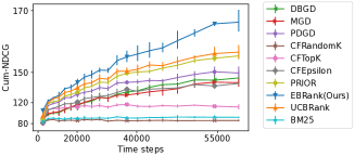
Figure 3. Ranking performance (MQ2007, W/-Behav setting).

As shown in Table 5.1.5, not all algorithms can benefit from incorporating behavior signals. Particularly, in Table 5.1.5, we indeed see that both W/-Behav(Concate) and W/-Behav(Non-Concate) feature settings help to boost most ranking algorithms to have better Warm-NDCG and Cum-NDCG. However, such boosting on Warm-NDCG and Cum-NDCG does not apply to all ranking algorithms, and there exist two exceptions. The first one is a trivial exception regarding CFRandomK. CFRandomK always randomly ranks items and shows them to users, so its online performance, i.e., Cum-NDCG, can not be boosted. The second one is a non-trivial exception regarding CFTopK. Incorporating user behaviors even makes CFTopK degenerate on Warm-NDCG and Cum-NDCG for all three datasets. Besides CFTopK’s degeneration on Warm-NDCG and Cum-NDCG, W/-Behav(Concate) feature setting even causes all ranking algorithms (except PRIOR) to experience a significant drop in Cold-NDCG, when compared to the W/o-Behav feature setting. Compared to other algorithms, UCBRank and our algorithm EBRank can benefit from behavior signals to have better Warm-NDCG and Cum-NDCG while avoiding drop in Cold-NDCG. In Table 5.1.5, PRIOR also avoids drop in Cold-NDCG but Prior is not as effective as UCBRank and EBRank in boosting Warm-NDCG and Cum-NDCG with user behavior. Besides the ranking performance in Table 5.1.5, we additionally show ranking performance as time steps increase in Figure 3. As shown in Figure 3, EBRank consistently outperforms baselines.

5.2.3. How do ranking algorithms suffer from exploitation bias?

In the above section, we found that there exists some exceptions, i.e., degeneration of ranking quality when using the W/-Behav(Concate) feature setting. In this section, we dig into the learned models to investigate the reason for the degeneration. To investigate the learned models, we output behavior and non-behavior features’ exploitation ratio for each algorithm in Table 4, where the $j^{th}$ feature’s exploitation ratio is defined as

(29) $$Ratio_{j}=\frac{|w_{j}|}{\sum_{i}|w_{i}|}$$

$w_{j}$ is the learned $j^{th}$ weight of a learned linear model. In Table 4, the behavior feature’s exploitation ratio is significantly greater than the non-behavior features’ ratio for all ranking algorithms, which makes behavior features overwhelm other non-behavior features, dominate the output, and discriminate cold-start items. The overwhelming effect will cause exploitation bias. Although the analysis is based on linear models, we believe non-linear models will make exploitation bias even more severe since non-linear models are even better at over-fitting the behavior features.

The exploitation bias is the reason for the ranking quality degeneration mentioned in the last Section (see Sec. 5.2.2). Specifically, CFTopK’s degeneration in Warm-NDCG and Cum-NDCG is because it fully trusts the exploitation biased ranking model without any exploration, which can discriminate against new items of high quality, making them hard to be discovered. Besides, the drop of Cold-NDCG under the W/-Behav(Concate) feature setting is because the exploitation-biased ranking model can not give an effective ranklist when behavior features are not available in the cold evaluation setting. Although behavior features also dominate in PRIOR, missing behavior feature is filled out by a behavior feature prediction model, which is the reason why its Cold-NDCG does not drop.

Table 4. Features’ exploitation ratio (Eq. 29) in the learnt linear model on dataset MQ2007. $x^{b}$ Ratio is the behavior features’ exploitation ratio. Max $x^{nb}$ Ratio is the maximum exploitation ratio of non-behavior features. Exploitation ratios for UCBRank, EBRank and BM25 are not included since they do not contain $x^{b}$ in their linear model.

Algorithms	$x^{b}$ Ratio	Max $x^{nb}$ Ratio
CFEpsilon	0.604(0.098)	0.071(0.038)
CFRandomK	0.498(0.067)	0.103(0.026)
CFTopK	0.591(0.087)	0.098(0.033)
DBGD	0.109(0.021)	0.063(0.019)
MGD	0.110(0.026)	0.062(0.018)
PDGD	0.623(0.037)	0.036(0.004)
PRIOR	0.572(0.105)	0.089(0.043)

Compared to those algorithms, EBRank is more robust to exploitation bias since it has comparable ranking performance on Cold-NDCG as algorithms using W/o-Behav and has superior performance on Warm-NDCG and Cum-NDCG. In other words, EBRank can take advantage of historical user behavior signals but is also robust to user behavior missing. Besides, EBRank also significantly outperforms UCBRank in Cum-NDCG and Warm-NDCG.

5.2.4. EBRank’s robustness to entering probability

.

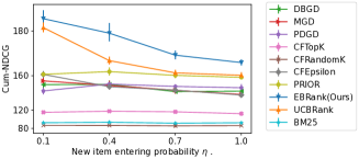
Figure 4. Ranking performance with different entering probability $\eta$ in simulation (see Eq. 28) on MQ2007. We only consider using user behavior situations here (except BM25).

To investigate the item entering speed ($\eta$) ’s influence on the ranking performance, we show the experimental results with different $\eta$ in Figure 4. As shown in Figure 4, EBRank consistently significantly outperforms all other algorithms under different item entering speeds.

5.2.5. Ablation Study

.

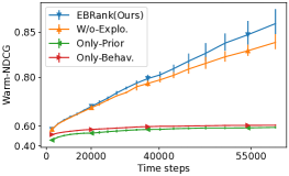
Figure 5. Ablation Study of EBRank on dataset MQ2007. W/o-Explo. means excluding $MC(d)$ in Eq. 13 when generating ranklists. Only-Prior means only using the prior model part $\frac{\alpha}{\alpha+\beta}$ of $\hat{R}$ (in Eq. 25) to rank items. Only-Behav. means only using the behavior part $\frac{C}{n}$ of $\hat{R}$ (in Eq. 25) to rank items.

In this section, we do an ablation study to see whether each part of our EBRank is needed. Due to limited space, we only provide analysis on MQ2007 dataset. As shown in Figure 5, EBRank significantly outperforms the version only using the Behavior part or the prior model part to rank. Also, from the ablation study, we observe Bayesian modeling can help a ranking model reach good ranking quality and be robust to exploitation bias. The marginal-certainty-aware exploration additionally helps to discover relevant items, which helps to boost ranking performance in the long term.

6. CONCLUSION

In this work, we propose an empirical Bayes-based uncertainty-aware ranking algorithm EBRank with the aim of overcoming the exploitation bias in LTR. With empirical Bayes modeling and a novel exploration strategy, EBRank aims to effectively overcome the exploitation bias and improve ranking quality. Extensive experiments on public datasets demonstrate that EBRank can achieve significantly better ranking performance than state-of-the-art LTR ranking algorithms. In the future, we plan to extend current work further to consider other types of user behaviors beyond user clicks.

References

- (1)
- Abramowitz and Stegun (1964) Milton Abramowitz and Irene A Stegun. 1964. Handbook of mathematical functions with formulas, graphs, and mathematical tables. Vol. 55. US Government printing office.
- Agarwal et al. (2019a) Aman Agarwal, Kenta Takatsu, Ivan Zaitsev, and Thorsten Joachims. 2019a. A general framework for counterfactual learning-to-rank. In Proceedings of the 42nd International ACM SIGIR Conference on Research and Development in Information Retrieval. 5–14.
- Agarwal et al. (2019b) Aman Agarwal, Ivan Zaitsev, Xuanhui Wang, Cheng Li, Marc Najork, and Thorsten Joachims. 2019b. Estimating position bias without intrusive interventions. In Proceedings of the Twelfth ACM International Conference on Web Search and Data Mining. 474–482.
- Agichtein et al. (2006) Eugene Agichtein, Eric Brill, and Susan Dumais. 2006. Improving web search ranking by incorporating user behavior information. In Proceedings of the 29th annual international ACM SIGIR conference on Research and development in information retrieval. 19–26.
- Ai et al. (2018a) Qingyao Ai, Keping Bi, Jiafeng Guo, and W Bruce Croft. 2018a. Learning a deep listwise context model for ranking refinement. In The 41st International ACM SIGIR Conference on Research & Development in Information Retrieval. 135–144.
- Ai et al. (2018b) Qingyao Ai, Keping Bi, Cheng Luo, Jiafeng Guo, and W Bruce Croft. 2018b. Unbiased learning to rank with unbiased propensity estimation. In The 41st International ACM SIGIR Conference on Research & Development in Information Retrieval. 385–394.
- Ai et al. (2021) Qingyao Ai, Tao Yang, Huazheng Wang, and Jiaxin Mao. 2021. Unbiased Learning to Rank: Online or Offline? ACM Transactions on Information Systems (TOIS) 39, 2 (2021), 1–29.
- Bekker et al. (2020) Jessa Bekker, Pieter Robberechts, and Jesse Davis. 2020. Beyond the selected completely at random assumption for learning from positive and unlabeled data. In Joint European Conference on Machine Learning and Knowledge Discovery in Databases. Springer, 71–85.
- Chapelle and Chang (2011) Olivier Chapelle and Yi Chang. 2011. Yahoo! learning to rank challenge overview. In Proceedings of the learning to rank challenge. PMLR, 1–24.
- Chapelle et al. (2009) Olivier Chapelle, Donald Metlzer, Ya Zhang, and Pierre Grinspan. 2009. Expected reciprocal rank for graded relevance. In Proceedings of the 18th ACM conference on Information and knowledge management. 621–630.
- Cief et al. (2022) Matej Cief, Branislav Kveton, and Michal Kompan. 2022. Pessimistic Off-Policy Optimization for Learning to Rank. arXiv preprint arXiv:2206.02593 (2022).
- Cohen et al. (2021) Daniel Cohen, Bhaskar Mitra, Oleg Lesota, Navid Rekabsaz, and Carsten Eickhoff. 2021. Not All Relevance Scores are Equal: Efficient Uncertainty and Calibration Modeling for Deep Retrieval Models. arXiv preprint arXiv:2105.04651 (2021).
- Craswell et al. (2008) Nick Craswell, Onno Zoeter, Michael Taylor, and Bill Ramsey. 2008. An experimental comparison of click position-bias models. In Proceedings of the 2008 international conference on web search and data mining. 87–94.
- Culpepper et al. (2016) J Shane Culpepper, Charles LA Clarke, and Jimmy Lin. 2016. Dynamic cutoff prediction in multi-stage retrieval systems. In Proceedings of the 21st Australasian Document Computing Symposium. 17–24.
- Dato et al. (2016) Domenico Dato, Claudio Lucchese, Franco Maria Nardini, Salvatore Orlando, Raffaele Perego, Nicola Tonellotto, and Rossano Venturini. 2016. Fast ranking with additive ensembles of oblivious and non-oblivious regression trees. ACM Transactions on Information Systems (TOIS) 35, 2 (2016), 1–31.
- Dempster et al. (1977) Arthur P Dempster, Nan M Laird, and Donald B Rubin. 1977. Maximum likelihood from incomplete data via the EM algorithm. Journal of the Royal Statistical Society: Series B (Methodological) 39, 1 (1977), 1–22.
- Gao et al. (2009) Jianfeng Gao, Wei Yuan, Xiao Li, Kefeng Deng, and Jian-Yun Nie. 2009. Smoothing clickthrough data for web search ranking. In Proceedings of the 32nd international ACM SIGIR conference on Research and development in information retrieval. 355–362.
- Gupta et al. (2020) Parth Gupta, Tommaso Dreossi, Jan Bakus, Yu-Hsiang Lin, and Vamsi Salaka. 2020. Treating Cold Start in Product Search by Priors. In Companion Proceedings of the Web Conference 2020. 77–78.
- Han et al. (2022) Cuize Han, Pablo Castells, Parth Gupta, Xu Xu, and Vamsi Salaka. 2022. Addressing Cold Start in Product Search via Empirical Bayes. In Proceedings of the 31st ACM International Conference on Information and Knowledge Management (Atlanta, GA, USA) (CIKM ’22). Association for Computing Machinery, New York, NY, USA, 3141–3151. https://doi.org/10.1145/3511808.3557066
- Järvelin and Kekäläinen (2002) Kalervo Järvelin and Jaana Kekäläinen. 2002. Cumulated gain-based evaluation of IR techniques. ACM Transactions on Information Systems (TOIS) 20, 4 (2002), 422–446.
- Jeunen and Goethals (2021) Olivier Jeunen and Bart Goethals. 2021. Pessimistic reward models for off-policy learning in recommendation. In Proceedings of the 15th ACM Conference on Recommender Systems. 63–74.
- Joachims et al. (2017) Thorsten Joachims, Adith Swaminathan, and Tobias Schnabel. 2017. Unbiased learning-to-rank with biased feedback. In Proceedings of the Tenth ACM International Conference on Web Search and Data Mining. 781–789.
- Kveton et al. (2022) Branislav Kveton, Ofer Meshi, Masrour Zoghi, and Zhen Qin. 2022. On the Value of Prior in Online Learning to Rank. In International Conference on Artificial Intelligence and Statistics. PMLR, 6880–6892.
- Li et al. (2020) Chang Li, Branislav Kveton, Tor Lattimore, Ilya Markov, Maarten de Rijke, Csaba Szepesvári, and Masrour Zoghi. 2020. BubbleRank: Safe online learning to re-rank via implicit click feedback. In Uncertainty in Artificial Intelligence. PMLR, 196–206.
- Liang and Vlassis (2022) Dawen Liang and Nikos Vlassis. 2022. Local Policy Improvement for Recommender Systems. arXiv preprint arXiv:2212.11431 (2022).
- Lien et al. (2019) Yen-Chieh Lien, Daniel Cohen, and W Bruce Croft. 2019. An assumption-free approach to the dynamic truncation of ranked lists. In Proceedings of the 2019 ACM SIGIR International Conference on Theory of Information Retrieval. 79–82.
- Liu et al. (2009) Tie-Yan Liu et al. 2009. Learning to rank for information retrieval. Foundations and Trends® in Information Retrieval 3, 3 (2009), 225–331.
- Macdonald et al. (2012) Craig Macdonald, Rodrygo LT Santos, and Iadh Ounis. 2012. On the usefulness of query features for learning to rank. In Proceedings of the 21st ACM international conference on Information and knowledge management. 2559–2562.
- Morik et al. (2020) Marco Morik, Ashudeep Singh, Jessica Hong, and Thorsten Joachims. 2020. Controlling Fairness and Bias in Dynamic Learning-to-Rank. In Proceedings of the 43rd International ACM SIGIR Conference on Research and Development in Information Retrieval (Virtual Event, China) (SIGIR ’20). Association for Computing Machinery, New York, NY, USA, 429–438. https://doi.org/10.1145/3397271.3401100
- Oosterhuis and de Rijke (2018) Harrie Oosterhuis and Maarten de Rijke. 2018. Differentiable unbiased online learning to rank. In Proceedings of the 27th ACM International Conference on Information and Knowledge Management. 1293–1302.
- Oosterhuis and de Rijke (2020) Harrie Oosterhuis and Maarten de Rijke. 2020. Policy-aware unbiased learning to rank for top-k rankings. In Proceedings of the 43rd International ACM SIGIR Conference on Research and Development in Information Retrieval. 489–498.
- Oosterhuis and de Rijke (2021a) Harrie Oosterhuis and Maarten de Rijke. 2021a. Unifying Online and Counterfactual Learning to Rank: A Novel Counterfactual Estimator that Effectively Utilizes Online Interventions. In Proceedings of the 14th ACM International Conference on Web Search and Data Mining. 463–471.
- Oosterhuis and de Rijke (2021b) Harrie Oosterhuis and Maarten de de Rijke. 2021b. Robust Generalization and Safe Query-Specializationin Counterfactual Learning to Rank. In Proceedings of the Web Conference 2021. 158–170.
- Ovaisi et al. (2020) Zohreh Ovaisi, Ragib Ahsan, Yifan Zhang, Kathryn Vasilaky, and Elena Zheleva. 2020. Correcting for selection bias in learning-to-rank systems. In Proceedings of The Web Conference 2020. 1863–1873.
- Penha and Hauff (2021) Gustavo Penha and Claudia Hauff. 2021. On the Calibration and Uncertainty of Neural Learning to Rank Models for Conversational Search. In Proceedings of the 16th Conference of the European Chapter of the Association for Computational Linguistics: Main Volume. 160–170.
- Qin et al. (2010) Tao Qin, Tie-Yan Liu, Jun Xu, and Hang Li. 2010. LETOR: A benchmark collection for research on learning to rank for information retrieval. Information Retrieval 13, 4 (2010), 346–374.
- Raiffa et al. (1961) Howard Raiffa, Robert Schlaifer, et al. 1961. Applied statistical decision theory. (1961).
- Roitman et al. (2017) Haggai Roitman, Shai Erera, and Bar Weiner. 2017. Robust standard deviation estimation for query performance prediction. In Proceedings of the ACM SIGIR International Conference on Theory of Information Retrieval. 245–248.
- Saito et al. (2020) Yuta Saito, Suguru Yaginuma, Yuta Nishino, Hayato Sakata, and Kazuhide Nakata. 2020. Unbiased recommender learning from missing-not-at-random implicit feedback. In Proceedings of the 13th International Conference on Web Search and Data Mining. 501–509.
- Schuth et al. (2013) Anne Schuth, Katja Hofmann, Shimon Whiteson, and Maarten de Rijke. 2013. Lerot: An online learning to rank framework. In Proceedings of the 2013 workshop on Living labs for information retrieval evaluation. 23–26.
- Schuth et al. (2016) Anne Schuth, Harrie Oosterhuis, Shimon Whiteson, and Maarten de Rijke. 2016. Multileave gradient descent for fast online learning to rank. In Proceedings of the Ninth ACM International Conference on Web Search and Data Mining. 457–466.
- Singh and Joachims (2018) Ashudeep Singh and Thorsten Joachims. 2018. Fairness of exposure in rankings. In Proceedings of the 24th ACM SIGKDD International Conference on Knowledge Discovery & Data Mining. 2219–2228.
- Smucker et al. (2007) Mark D Smucker, James Allan, and Ben Carterette. 2007. A comparison of statistical significance tests for information retrieval evaluation. In Proceedings of the sixteenth ACM conference on Conference on information and knowledge management. 623–632.
- Tran et al. (2021) Anh Tran, Tao Yang, and Qingyao Ai. 2021. ULTRA: An Unbiased Learning To Rank Algorithm Toolbox. In Proceedings of the 30th ACM International Conference on Information & Knowledge Management. 4613–4622.
- Vardasbi et al. (2020) Ali Vardasbi, Harrie Oosterhuis, and Maarten de Rijke. 2020. When Inverse Propensity Scoring does not Work: Affine Corrections for Unbiased Learning to Rank. In Proceedings of the 29th ACM International Conference on Information & Knowledge Management. 1475–1484.
- Wang et al. (2019) Huazheng Wang, Sonwoo Kim, Eric McCord-Snook, Qingyun Wu, and Hongning Wang. 2019. Variance reduction in gradient exploration for online learning to rank. In Proceedings of the 42nd International ACM SIGIR Conference on Research and Development in Information Retrieval. 835–844.
- Wang et al. (2018b) Huazheng Wang, Ramsey Langley, Sonwoo Kim, Eric McCord-Snook, and Hongning Wang. 2018b. Efficient exploration of gradient space for online learning to rank. In The 41st International ACM SIGIR Conference on Research & Development in Information Retrieval. 145–154.
- Wang et al. (2021) Qunbo Wang, Wenjun Wu, Yuxing Qi, and Yongchi Zhao. 2021. Deep bayesian active learning for learning to rank: A case study in answer selection. IEEE Transactions on Knowledge and Data Engineering (2021).
- Wang et al. (2016) Xuanhui Wang, Michael Bendersky, Donald Metzler, and Marc Najork. 2016. Learning to rank with selection bias in personal search. In Proceedings of the 39th International ACM SIGIR conference on Research and Development in Information Retrieval. 115–124.
- Wang et al. (2018a) Xuanhui Wang, Nadav Golbandi, Michael Bendersky, Donald Metzler, and Marc Najork. 2018a. Position bias estimation for unbiased learning to rank in personal search. In Proceedings of the Eleventh ACM International Conference on Web Search and Data Mining. 610–618.
- Yang and Ai (2021) Tao Yang and Qingyao Ai. 2021. Maximizing marginal fairness for dynamic learning to rank. In Proceedings of the Web Conference 2021. 137–145.
- Yang et al. (2020) Tao Yang, Shikai Fang, Shibo Li, Yulan Wang, and Qingyao Ai. 2020. Analysis of multivariate scoring functions for automatic unbiased learning to rank. In Proceedings of the 29th ACM International Conference on Information & Knowledge Management. 2277–2280.
- Yang et al. (2022) Tao Yang, Chen Luo, Hanqing Lu, Parth Gupta, Bing Yin, and Qingyao Ai. 2022. Can clicks be both labels and features? Unbiased Behavior Feature Collection and Uncertainty-aware Learning to Rank. In Proceedings of the 45th International ACM SIGIR Conference on Research and Development in Information Retrieval. 6–17.
- Yang et al. (2023) Tao Yang, Zhichao Xu, Zhenduo Wang, Anh Tran, and Qingyao Ai. 2023. Marginal-Certainty-aware Fair Ranking Algorithm. In Proceedings of the Sixteenth ACM International Conference on Web Search and Data Mining. 24–32.
- Yue and Joachims (2009) Yisong Yue and Thorsten Joachims. 2009. Interactively optimizing information retrieval systems as a dueling bandits problem. In Proceedings of the 26th Annual International Conference on Machine Learning. 1201–1208.
- Zhu et al. (2009) Jianhan Zhu, Jun Wang, Michael Taylor, and Ingemar J Cox. 2009. Risk-aware information retrieval. In European Conference on Information Retrieval. Springer, 17–28.
- Zoghi et al. (2017) Masrour Zoghi, Tomas Tunys, Mohammad Ghavamzadeh, Branislav Kveton, Csaba Szepesvari, and Zheng Wen. 2017. Online learning to rank in stochastic click models. In International Conference on Machine Learning. PMLR, 4199–4208.