Emergence of pseudo-time during optimal Monte Carlo sampling
and temporal aspects of symmetry breaking and restoration

Abstract

We argue that one can associate a pseudo-time with sequences of configurations generated in the course of classical Monte Carlo simulations for a single-minimum bound state, if the sampling is optimal. Hereby the sampling rates can be, under special circumstances, calibrated against the relaxation rate and frequency of motion of an actual physical system. The latter possibility is linked to the optimal sampling regime being a universal crossover separating two distinct suboptimal sampling regimes analogous to the physical phenomena of diffusion and effusion, respectively. Bound states break symmetry; one may thus regard the pseudo-time as a quantity emerging together with the bound state. Conversely, when transport among distinct bound states takes place—thus restoring symmetry—a pseudo-time can no longer be defined. One can still quantify activation barriers, if the latter barriers are smooth, but the simulation becomes impractically slow and pertains to overdamped transport only. Specially designed Monte Carlo moves that bypass activation barriers—so as to accelerate sampling of the thermodynamics—amount to effusive transport and lead to severe under-sampling of transition-state configurations that separate distinct bound states while destroying the said universality. Implications of the present findings for simulations of glassy liquids are discussed.

I Motivation

The thermodynamics of a classical system can be efficiently quantified by Gibbs-sampling its Boltzmann distribution Newman and Barkema (1999); Socci, Onuchic, and Wolynes (1996); Berthier and Reichman (2023); Rossky, Doll, and Friedman (1978) because the sampled variables are not subject to inertia. Microscopic characterization of transition states for activated escape from bound states, then, poses a challenge: To quantify rates of escape, one must evaluate autocorrelations for quantities sampled at well-defined intervals of time. Yet it is not clear to what extent sequences of configurations generated using classical Monte Carlo (MC) simulation Newman and Barkema (1999) correspond with actual dynamics, if at all. There is also the distinct possibility that the transition states—which often contribute negligibly little to thermodynamics—are not adequately represented during statistical sampling thus preventing one from quantifying their microscopic characteristics such as the extent of cooperativity.

At the same time, correlation functions generated in the course of Monte Carlo sampling of the Boltzmann distribution for a classical system often look qualitatively similar to correlation functions measured in experiment. Thus one may reasonably inquire Bal and Neyts (2014); Kikuchi et al. (1991); Berthier and Kob (2007) whether there are conditions under which there may be a quantitative connection between the apparent kinetics observed, respectively, in Monte Carlo simulations and the actual molecular dynamics. One may immediately object that already the lack of inertia intrinsic to statistical sampling introduces too much ambiguity because masses of individual particles and collective modes, if any, are generally distributed. But the latter ambiguity may be only semi-quantitative since a particle’s proper time is scaled by the square-root of the particle’s mass, while in many systems of interest Socci, Onuchic, and Wolynes (1996) the masses of what one would ordinarily define as particles vary only modestly. For instance, a methyl group weighs 15 Dalton, the amino group 17, the hydroxy group 17, etc. In any event, the ambiguity due to mass variation, if any, is often much smaller than the dynamic range of six orders of magnitude—and usually more—that is found in many contexts of practical interest, such as dynamics of glassy liquids. Lubchenko (2015); Lubchenko and Wolynes (2007)

Accelerated Monte Carlo protocols—such as those employing peculiar moves that swap particles’ places in glassy mixtures Ninarello, Berthier, and Coslovich (2017); Berthier and Reichman (2023); Berthier et al. (2019a, b)—seem to be particularly efficient at sampling the thermodynamics very deep in the free energy landscape, where physical moves would be subject to high activation barriers. Lubchenko (2015); Lubchenko and Wolynes (2007); Scalliet, Guiselin, and Berthier (2022) Clearly, this efficiency is predicated on the ability of an accelerated protocol to circumvent the transition states for such activated processes. This, then, prompts one to examine to what extent accelerated protocols sample those transition states or might allow one to quantify their microscopic characteristics.

Here we argue that notwithstanding the apparent similarity of MC-produced relaxation profiles to physical relaxations, one can not associate the time-step of Monte Carlo sampling with a physical time in systems characterized by a distribution of length and time scales. Such distribution is characteristic of most applications of practical interest, of course. Only under some special circumstances can one define a pseudo-time for simulated sequences of variables so that the time interval separating two consecutively sampled configurations can be connected to the relaxation time and/or vibrational period of a bound motion in an actual system. That such special circumstances could arise can be understood by combining the following two notions:

On the one hand, configurations sampled during physical processes near equilibrium are such that the rate of entropy increase is at its maximum possible value, per Onsager. Onsager (1931a, b) Thus the set of physical configurations statistically relevant for processes near equilibrium also correspond to the optimal rate of equilibration. At the same time, equilibrium from the statistical viewpoint corresponds to the degrees of freedom strictly obeying the Boltzmann distribution. Thus maximum entropy production is equivalent to the rate of sampling of the Boltzmann distribution being optimal.

On the other hand, the question of the optimal rate of Gibbs sampling of probability distributions is well defined and, furthermore, can be answered rather accurately in many cases of practical interest, see Ref. Roberts and Rosenthal (2001) and references therein. The optimal regime of sampling emerges as a compromise between the length of attempted increments of the sampled variable, on the one hand, and the acceptance rate for attempted moves, on the other hand. Suppose the increment is Gaussianly distributed with standard deviation $l$ while the Boltzmann distribution is a univariate Gaussian distribution with standard deviation $\sigma$. The optimal step size Roberts and Rosenthal (2001) is, apparently, rather large, $l\approx 2.4\>\sigma$, suggesting the continuity of actual physical trajectories may be statistically redundant under certain circumstances. To see that such redundancy is plausible, consider an equilibrated, mechanically-stable solid composed of hard spheres. One can approximately associate the Monte Carlo step size with the distance traveled between consecutive collisions and, thus, the typical step size should be comparable to the double of the r.m.s.d. for the vibrational motion of a given particle, within the cage created by the surrounding particles. Motions between consecutive collisions are straight lines that can be generically reconstructed, since the typical speed is fixed by temperature.

Motivated by the notions above, one might further ask to what extent Monte Carlo-generated correlation functions could also reflect the kinetics of activated transitions among distinct bound states, and to what extent the sampled configurations could reflect the morphology of the corresponding transition states. This is a question of considerable interest in systems exhibiting free energy surfaces with multiple minima, such as glassy liquids. Lubchenko (2015) In the presence of activated processes, relaxation functions show two distinct, time-separated processes: Mezei and Russina (1999) The faster process presumably corresponds to vibrational relaxation within individual free energy minima, while the slower process corresponds to activated escapes from those free-energy minima. Lubchenko (2015); Lubchenko and Wolynes (2007, 2012) If one could connect Monte Carlo sampling of individual bound states to the actual vibrational dynamics, one could perhaps use the corresponding sampling rates as a reference timescale to systematically quantify the lifetimes of bound states. It would be of value, too, if one could calibrate activated kinetics—by using vibrational relaxation rates as the reference—to compare results of simulations across systems with different force fields.

In addressing these questions, we proceed as follows: In Section II, we first construct an explicit semi-Markov process corresponding to the Metropolis variety of Monte-Carlo sampling, which allows one to associate a continuous time-like variable to the intrinsically discrete process of statistical sampling. We show that the two extreme limits of a very small and very large size of attempted displacements are analogous to physical phenomena of diffusion and effusion, respectively. At the crossover between the two regimes, the sampling rate or, equivalently, the relaxation rate reaches its optimal value. At the same time, universal relationships emerge between the time interval of the simulation—which is à priori an arbitrary parameter—and the apparent relaxation rate, as well as the frequency of motion within a single-well bound state. We then outline the special circumstances under which the aforementioned time variable of the semi-Markov process can be thought of as a pseudo-physical time. The crossover is also linked to the appearance of a well-defined gap separating the two largest eigenvalues of the transition matrix for the Markov chain corresponding to the Monte Carlo sampling. In Section III, we show that notwithstanding the apparent causal connection among the configurations generated during optimal sampling, the latter configurations cannot be interpreted as snapshots of continuous trajectories, thus greatly limiting one’s ability to sample transitions states separating distinct bound states. There we also discuss ambiguities, inherent to Monte Carlo simulations, that stem from the distribution of particles’ masses. The above findings are explicitly illustrated in Section IV using both analytical estimates and direct simulation. There, we show that in the presence of activated transport, a pseudo-time cannot be defined. In the strict diffusion limit and for sufficiently smooth barrier tops, one can still hope to recover correct activation energies. The diffusion limit—in which the trajectories become effectively continuous, though non-inertial—is however computationally inefficient. Moves designed to speed up sampling also lead to a loss of the connection between optimal sampling of individual bound states and vibrational relaxation. Furthermore, such accelerated protocols result in severe under-sampling of transition states for activated transport and underestimation of activation barriers. Finally we discuss implications of the present results for the ongoing efforts to elucidate the detailed mechanism of activated transport in glassy liquids.

II Monte Carlo simulation as a semi-Markov process, and emergence of optimal sampling

First we define a Markov chain with stationary transition probabilities Ross (1992) whose sole purpose is to mutually connect a set of physical states of interest, irrespective of the long-term probability to reside in any one of those states. Thus we introduce a transition matrix that specifies the probability to be in state $j$ at step number $N+1$, if the system was in state $i$ at step number $N$, irrespective of the prior history:

$$q_{ji}\equiv q(j\leftarrow i).$$ (1)

In the context of Monte Carlo (MC) simulation, the matrix $q_{ji}$ specifies the set of trial moves that could be attempted, in principle, during sampling and is often called the “proposal density.” We are exclusively interested in probability conserving processes. That is,

$$\sum_{j}q_{ji}=1,$$ (2)

for all $i$’s. Note the above conventions for the order of the matrix indices are the opposite of what is often adopted in statistics. Within the present conventions, all operators consistently apply to the right, as would the conventional derivative, for instance.

One may further ask: Can one modify the proposals specified by the matrix $q_{ji}$ so that the resulting transition matrix $\pi_{ji}$ yields a pre-specified stationary probability distribution of choice: $p_{i}$, $\sum_{i}p_{i}=1$? The sought transition matrix must obey detailed balance:

$$\pi_{ji}p_{i}=\pi_{ij}p_{j}.$$ (3)

Per Hastings, Hastings (1970) there are an infinite number of prescriptions to accomplish this task. Hereby one introduces a new quantity $\alpha_{ji}$, often called the “acceptance rate”, that multiplies the off-diagonal elements of the proposal matrix to yield the off-diagonal elements of the sought matrix $\pi_{ji}$:

$$\pi_{ji}=\alpha_{ji}q_{ji},j\neq i$$ (4)

while setting the diagonal element so as to ensure probability conservation:

$$\pi_{ii}=1-\sum_{j\neq i}\pi_{ji}$$ (5)

The following prescription for the acceptance rate:

$$\alpha_{ji}=\left\{\begin{array}[]{ll}1,&\frac{q_{ij}p_{j}}{q_{ji}p_{i}}\geq 1\\ \\ \frac{q_{ij}p_{j}}{q_{ji}p_{i}},&\frac{q_{ij}p_{j}}{q_{ji}p_{i}}<1\end{array}\right.$$ (6)

together with a symmetric proposal density:

$$q_{ij}=q_{ji}$$ (7)

yield the venerable Metropolis selection criterion: Metropolis et al. (1953)

$$\alpha_{ji}=\left\{\begin{array}[]{ll}1,&\frac{p_{j}}{p_{i}}\geq 1\\ \\ \frac{p_{j}}{p_{i}},&\frac{p_{j}}{p_{i}}<1\end{array}\right.$$ (8)

One may parametrize the probability distribution $p_{i}$, without loss of generality, as a Boltzmann distribution using an energy-like parameter $E_{i}$:

$$p_{i}\propto e^{-\beta E_{i}}\equiv e^{-E_{i}/k_{B}T}$$ (9)

where $T\equiv 1/k_{B}\beta$ stands for temperature. For the sake of completeness we note that bound states generally have both enthalpic and entropic contributions. Consequently, the appropriate energy $E_{i}$ could include the isobaric contribution $pV_{i}$ and/or grand-canonical contribution $(-\mu N_{i})$, where $p$ stands for pressure, $V$ volume, $\mu$ the chemical potential, and $N$ particle number.

It will be convenient to introduce an auxiliary function

$$B(j\leftarrow i)\equiv\left\{\begin{array}[]{ll}1,&E_{j}\leq E_{i}\\ \\ e^{-\beta(E_{j}-E_{i})},&E_{j}>E_{i}\end{array}\right.$$ (10)

which is simply the acceptance ratio for the Metropolis algorithm complemented by the value $B(i\leftarrow i)=1$; the function $B(j\leftarrow i)$ is thus continuous with respect to both arguments. Using an arrow in the notation is unconventional yet it seems to make algebraic manipulations more vivid.

Eqs. (4)-(10) can be consolidated to yield the following expression for the sought transition matrix:

$$\pi_{ji} =q_{ij}B(j\leftarrow i),\hskip 8.53581pt(j\neq i)$$ (11)

$$\pi_{jj} =q_{jj}B(j\leftarrow j)+\sum_{k}q_{jk}[1-B(k\leftarrow j)]$$

$$=1+q_{jj}B(j\leftarrow j)-\sum_{k}q_{jk}B(k\leftarrow j),$$ (12)

where we used Eqs. (2) and (7). Note the summation over $k$ in Eq. (12) is unrestricted.

One may further associate a semi-Markov process Ross (1992) to the transition matrix $\pi_{ji}$ by specifying a distribution $\psi_{ji}(t)$ of wait (or, interarrival) times $t$ for each of the $i\to j$ transitions; the latter distributions must each be normalized $\int dt\,\psi_{ji}(t)=1$. One may model an arbitrary process by specifying an appropriate set of functions $\psi_{ji}(t)$. One thus obtains the probability $P_{ji}(t)$ of being in state $j$ at time $t$ given the particle was in state $i$ at time zero. At any time, $\sum_{j}P_{ji}(t)=1$. Although we will often refer to the time-variable $t$ of the semi-Markov process simply as “time,” for brevity, it is unrelated to physical time except under special circumstances, see below.

If one specifies such initial conditions that at time zero: $P_{ij}(0)=\delta_{ij}$, the matrix ${\bm{P}}(t)\equiv\{P_{ij}(t)\}$ can be thought of as a Green’s function. Indeed, the latter matrix yields the population pattern in the system at time $t$: ${\bm{p}}(t)={\bm{P}}(t){\bm{p}}(0)$, where ${\bm{p}}(t)\equiv[p_{1}(t)\>\>p_{2}(t)\ldots]^{T}$ is a column whose entries are state populations $p_{i}(t)$ at time $t$. The Laplace transform of the probability, $\widetilde{\bm{P}}(s)=\int_{0}^{\infty}dt\,e^{-st}{\bm{P}}(t)$, can be expressed in terms of the transition-matrix elements $\pi_{ij}$ and the Laplace transforms of the functions $\psi_{ij}$, through a well known formula,Ross (1992) see also Ref. Lubchenko and Silbey (2004):

$$\widetilde{\bm{P}}(s)^{-1}|_{ij}=[\delta_{ij}-\pi_{ij}\widetilde{\psi}_{ij}(s)]\frac{s}{1-\sum_{k}\pi_{kj}\widetilde{\psi}_{kj}(s)}.$$ (13)

The formal expression (13) is generally intractable but simplifies greatly when the waiting time distribution depends only on the identity of the originating site: $\psi_{ji}(t)=\psi_{i}(t)$. Here, we are interested in the simpler yet, fully uniform case

$$\psi_{ij}(t)=\psi(t).$$ (14)

Hereby we assign a distributed, temporal-like interval to each Monte Carlo step where the assignment is independent of the current configuration of the system. Under the constraint from Eq. (14), Eq. (13) yields:

$$s\widetilde{\bm{P}}(s)-{\bm{1}}=\frac{s\widetilde{\psi}(s)}{1-\widetilde{\psi}(s)}({\bm{\pi}}-{\bm{1}})\widetilde{\bm{P}}(s)$$ (15)

where ${\bm{\pi}}$ is the shorthand for the square matrix composed of elements $\pi_{ij}$ and ${\bm{1}}$ is the unit matrix.

In conventional Monte Carlo simulations, one simply uses the step number as the effective time variable:

$$\psi_{\mbox{\tiny MC}}(t)=\delta(t-\Delta t)$$ (16)

where $\Delta t=1$. We will adhere to this convention when performing Monte Carlo simulations as well. For calculations, on the other hand, it is more convenient to make the time $t$ of the semi-Markov process a continous variable, in a statistical sense, by adopting a smooth probability density that is non-vanishing at the origin. To this end, we will adopt the Poisson statistics:

$$\psi(t)=\frac{1}{\Delta t}e^{-t/\Delta t}.$$ (17)

The parameter $\Delta t$ is now seen to specify the average waiting time for the semi-Markov process. Eq. (15) immediately gives a first-order differential equation for the survival probabilities, in terms of a continuous, time-like variable $t$:

$$\dot{{\bm{P}}}(t)=\frac{1}{\Delta t}({\bm{\pi}}-{\bm{1}})\,{\bm{P}}(t)$$ (18)

and the initial condition ${\bm{P}}(t=0)={\bm{1}}$. Equivalently, one may directly write down a differential equation for a probability distribution

$$\dot{{\bm{p}}}(t)=\frac{1}{\Delta t}({\bm{\pi}}-{\bm{1}})\,{\bm{p}}(t)$$ (19)

where one must specify the initial condition ${\bm{p}}(t=0)$.

Within the assumptions that led to Eq. (19), the question of the apparent rate of Monte Carlo sampling is reduced to the question of the eigenvalues of the matrix ${\bm{\pi}}$. The largest eigenvalue, $\lambda_{1}=1$, has the equilibrium probability distribution as its eigenvector, per Eqs. (3) and (5). The corresponding relaxation rate vanishes: $-(\lambda_{1}-1)=(1-\lambda_{1})=0$. Consider now the next largest eigenvalue, $\lambda_{2}$. The quantity $(1-\lambda_{2})$ yields the lower bound on the rate at which the apparent distribution approaches its equilibrium value, according to Eq. (19). As such, the quantity $(1-\lambda_{2})$ also measures the efficiency of sampling. This is also a good place to elaborate on the effect of a specific choice of the functional form for the wait-time distribution $\psi$. Suppose we use an eigenvector corresponding to some eigenvalue $\lambda$ of the matrix ${\bm{\pi}}$ as the initial condition for the semi-Markov process. For the discrete prescription from Eq. (16), the probability value after $N$ events is $p(N=t/\Delta t)=\lambda^{N}p(t=0)=e^{t\ln\lambda/\Delta t}p(t=0)$, which nominally corresponds to the rate $(-\ln\lambda/\Delta t)$. On the other hand, the Poisson prescription from Eq. (17) gives $p(t)=e^{-(1-\lambda)t/\Delta t}p(t=0)$, per Eq. (19), which corresponds to the rate $(1-\lambda)/\Delta t$. The quantities $(-\ln\lambda)$ and $(1-\lambda)$ both monotonically decrease with $\lambda$, and so the difference between these two specific prescriptions for the distribution $\psi$ of the wait times does not affect the discussion of the efficiency of sampling in a substantive way. In any event, the rates $(-\ln\lambda)$ and $(1-\lambda)$ approach each other asymptotically in the $\lambda\to 1$ limit and are numerically close even in the worst-case scenario, as we shall see below. Other forms for the wait-time distribution $\psi$ could be considered, in principle. For the reader’s reference, we show in Appendix A that the Laplace transform of the relaxation profile for eigenvectors corresponding to an eigenvalue $\lambda$, for an arbitrary $\psi(t)$, is given by a rather simple equation:

$$\widetilde{p}_{\lambda}(s)=\frac{1}{s}\>\frac{1-\widetilde{\psi}(s)}{1-\lambda\widetilde{\psi}(s)}$$ (20)

Although the resulting relaxation profile $p_{\lambda}(t)$ can be quite complicated—depending on the specific form of $\widetilde{\psi}(s)$—we see it is always slower for higher values of $\lambda$. In any event, it seems prudent to avoid $\psi$’s with long tails unless slow processes are known to be present.

Next we ask whether there are circumstances under which the time-like quantity $t$ may be connected to actual physical time. To this end, we explicitly rewrite Eq. (18) for a process in which individual sites are each associated with a location in space of dimensionality $d$. The latter dimensionality may or may not be equal to the number of physical dimensions. And so, for instance, if one attempts to move two particles at a time, in the actual physical space, the dimensionality of the semi-Markov process is six. Going over to continuous variables, ${\bm{P}}_{ij}\to P({\bm{x}},{\bm{z}})$ etc., Eqs. (11)-(12) and (18) straightforwardly yield:

$$\dot{P}({\bm{y}},{\bm{z}}) =\frac{1}{\Delta t}\int d^{d}{\bm{x}}\>q({\bm{x}},{\bm{y}})$$

$$\times[B({\bm{y}}\leftarrow{\bm{x}})P({\bm{x}},{\bm{z}})-B({\bm{x}}\leftarrow{\bm{y}})P({\bm{y}},{\bm{z}})]$$ (21)

and initial condition $P({\bm{y}},{\bm{z}})_{t=0}=\delta^{(d)}({\bm{y}}-{\bm{z}})$, where $\delta^{(d)}$ is the $d$-dimensional Dirac delta-function. The above equation can be equivalently rewritten as an integro-differential equation for a function of a single set of coordinates:

$$\dot{p}({\bm{y}})=\frac{1}{\Delta t}\int\!d^{d}{\bm{x}}\hskip 1.42262ptq({\bm{x}},{\bm{y}})[B({\bm{y}}\leftarrow{\bm{x}})p({\bm{x}})-B({\bm{x}}\leftarrow{\bm{y}})p({\bm{y}})]$$ (22)

where the initial condition $p({\bm{y}},t=0)$ is user-specified. To emphasize that the contribution of the kinetic energy to the total energy is not included in classical Monte Carlo sampling, from here on we switch notations as follows:

$$E_{i}\to V(x)$$ (23)

It may be sometimes more convenient to rewrite Eq. (22) for an auxiliary function defined as

$$\widetilde{p}({\bm{x}})\equiv p({\bm{x}})e^{\beta V({\bm{x}})}$$ (24)

whereby deviations from equilibrium, if any, result in the function $\tilde{p}$ being spatially non-uniform. One thus obtains straightforwardly:

$$(\Delta t)\>\dot{\widetilde{p}}_{\bm{x}} =\int_{V_{\bm{y}}<V_{\bm{x}}}d^{d}{\bm{y}}\>(\widetilde{p}_{\bm{y}}-\widetilde{p}_{\bm{x}})q({\bm{x}},{\bm{y}})$$

$$+\int_{V_{\bm{y}}>V_{\bm{x}}}d^{d}{\bm{y}}\>(\widetilde{p}_{\bm{y}}-\widetilde{p}_{\bm{x}})e^{-\beta(V_{\bm{y}}-V_{\bm{x}})}q({\bm{x}},{\bm{y}})$$ (25)

and we have compactified notations for typographical clarity: $p_{x}\equiv p({\bm{x}})$, $V_{\bm{x}}\equiv V({\bm{x}})$, etc.

From here on, we adopt the translationally invariant, Gaussian proposal density:

$$q({\bm{x}},{\bm{y}})=\frac{1}{(2\pi l^{2})^{d/2}}e^{-\frac{({\bm{x}}-{\bm{y}})^{2}}{2l^{2}}}$$ (26)

where the quantity $l$ thus gives the r.m.s.d. of the distribution of the step size for attempted moves along a single spatial dimension.

In the ultra-local limit of a vanishing step size, one may Taylor-expand the function $\widetilde{p}_{y}$ in the integrands in Eq. (II) around $y=x$, which yields straightforwardly:

$$\dot{\widetilde{p}}=\frac{l^{2}}{2\Delta t}\left[\nabla^{2}\widetilde{p}-(\nabla\beta V)(\nabla\widetilde{p})\right].$$ (27)

Subsequently, this leads to the familiar Smoluchowski-Fokker-Planck equation Zwanzig (2001); van Kampen (1981) for the original probability density:

$$\dot{p}=D_{\mbox{\tiny MC}}\nabla e^{-\beta V}\nabla e^{\beta V}p$$ (28)

after we formally associate an effective diffusivity

$$D_{\mbox{\tiny MC}}\equiv\frac{l^{2}}{2\Delta t}$$ (29)

with the step size $l$ and the parameter $\Delta t$, consistent with Ref. Kikuchi et al. (1991) We use the label “MC” to emphasize that the quantity $D_{\mbox{\tiny MC}}$ is not a physical diffusivity. The Smoluchowski equation above formally corresponds to an overdamped Langevin dynamics, Goldenfeld (1992)

$$\zeta_{\mbox{\tiny MC}}\,\dot{{\bm{x}}}=-\frac{\partial V}{\partial{\bm{x}}}+{\bm{f}}_{\text{th}}$$ (30)

Where the quantity $\zeta_{\mbox{\tiny MC}}$ is an effective friction coefficient defined through the diffusivity (29) via an Einstein-like relation:

$$\zeta_{\mbox{\tiny MC}}=\frac{k_{B}T}{D_{\mbox{\tiny MC}}}$$ (31)

and ${\bm{f}}_{\text{th}}$ is the corresponding, effective fluctuating force needed for energy balance. For a $d$-dimensional oscillator:

$$V({\bm{x}})=\frac{kx^{2}}{2}$$ (32)

the overdamped Langevin dynamics yields, by Eq. (30), the following relaxation rate:

$$\frac{1}{\tau}=\frac{k}{\zeta_{\mbox{\tiny MC}}}=\frac{1}{2\Delta t}\left(\frac{l}{l_{\text{th}}}\right)^{2}$$ (33)

where we used Eqs. (29) and (31) and have introduced the thermal length $l_{\text{th}}$ that determines the r.m.s.d. for bound motions along an individual spatial direction, per the Boltzmann distribution corresponding to the energy function (32):

$$l_{\text{th}}\equiv\left(\frac{k_{B}T}{k}\right)^{1/2}.$$ (34)

When the step size $l$ becomes comparable to or greater than the length scale for spatial variation of the probability distribution, the long-wavelength expansion used to derive the Fokker-Planck equation is no longer valid, while the semi-Markov process corresponding to MC sampling can not be thought of as diffusion-like but, instead, becomes expressly non-local. While the integral equation (22) seems difficult to solve under general circumstances, the limit of large $l$, $l\gg l_{\text{th}}$, can be readily understood at a semi-quantitative level and, further, linked to the physical phenomenon of effusion. Indeed, in this limit, the region spanned by the equilibrium probability distribution is much smaller than the region typically traversed in one jump. For energy function (32), the acceptance rate for jumps out of a typical configuration, $\simeq\frac{l^{d}-l_{\text{th}}^{d}}{l^{d}}\,e^{-l^{2}/2l_{\text{th}}^{2}}\approx e^{-l^{2}/2l_{\text{th}}^{2}}$, is very low, implying the system will remain within bounds prescribed by the Boltzmann distribution most of the time, while the non-typical configurations will be populated roughly at $e^{-l^{2}/2l_{\text{th}}^{2}}$. It is instructive to group all the typical states into one set, call it A, while grouping the non-typical states into one set also, call the latter set B. Once in state B, the system is at distance $l$ or so from the typical location and will typically sample a region of volume $l^{d}$, up to a geometric factor, since all of this region corresponds to acceptance rates comparable to 1. Only a fraction $\approx(l_{\text{th}}/l)^{d}$ of these moves will bring the system back to state A, however, because the volume of the corresponding region is $l_{\text{th}}^{d}$, up to a geometric factor. This fraction, then, sets the sampling rate for the multivariate Gaussian distribution corresponding to the bound state described by Eq. (32), roughly at

$$\frac{1}{\tau}\sim\frac{1}{\Delta t}\left(\frac{l_{\text{th}}}{l}\right)^{d}.$$ (35)

where $l\gg l_{\text{th}}$. Thus the probability to “hit the spot” occupied by typical states is determined by the volume $l_{\text{th}}^{d}$ of the latter region in the same way the chance for a particle to effusively escape from a container is determined by the probability to hit the orifice, hence the effusion analogy.

A somewhat more systematic approach, see Appendix B, confirms the above scaling while also yielding a geometric factor that depends on the dimensionality of space:

$$\frac{1}{\tau}\approx\frac{1}{\Delta t}\left[\frac{2}{d}\>\frac{\Gamma(d)}{\Gamma^{2}(d/2)}+1\right]\left(\frac{l_{\text{th}}}{l}\right)^{d}.$$ (36)

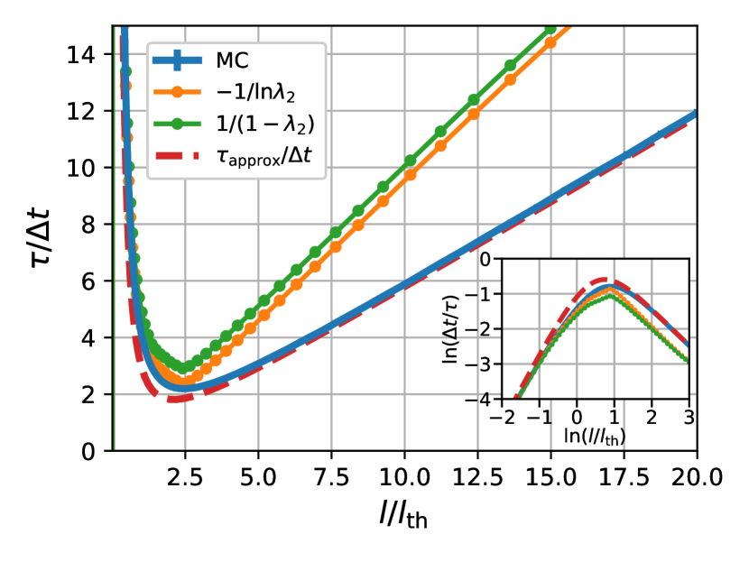
Figure 1: Thick solid line (“MC”): The longest relaxation time of the Monte-Carlo sampling of a harmonic bound state as a function of the step size relative to the thermal length, $l/l_{\text{th}}$. Thick dashed line (“$\tau_{\text{approx}}/\Delta t$”): $-1/\ln(1-\Delta t/\tau)$, where the $\Delta t/\tau$ ratio is computed according to the approximate relation (84) at $d=1$. Thin lines with dots show the result of direct diagonalization of the transition matrix of the Markov chain. We provide values for both the quantity $(1-\lambda_{2})$ and $-\ln\lambda_{2}$. The results of diagonalization become progressively inaccurate at large values of $l$ because of numerical issues. Inset: Log-log plots of the corresponding relaxation rates vs. $l/l_{\text{th}}$.

Thus the efficiency of sampling declines with the step size $l$ for large values of $(l/l_{\text{th}})$, the rate of the decline increasing with the dimensionality of the sampled variable. Combined with the low-$l$ scaling from Eq. (33), this means the sampling rate is maximized for some value of the $l/l_{\text{th}}$ ratio intermediate between the two asymptotic regimes described by Eqs. (33) and (36), respectively. The position of the crossover, then, fixes the dimensionless quantities $l/l_{\text{th}}$ and $\Delta t/\tau$ at some values that can depend only on the dimensionality $d$ of space and, thus, are universal. One can make an informal argument for the $d$-dependence of the optimal displacement by noting that a particle “moving” according to the proposal density (26) in $d$ dimensions tends to drift away from a given locale typically at the rate of $l\sqrt{d}$ per step. At optimal sampling, a single move should be able to traverse the thermally occupied region, whose size is about $2l_{\text{th}}$ across, irrespective of dimensionality. Thus we conclude that, roughly, $l_{\text{opt}}\simeq 2l_{\text{th}}/\sqrt{d}$ and that optimal sampling becomes increasingly diffusion-like in higher dimensions because the step size becomes progressively smaller than the length $l_{\text{th}}$ characterizing the spatial extent of the Boltzmann distribution.

The existence of a most efficient sampling rate had been established systematically quite a while ago,Roberts and Rosenthal (2001) of course. In addition to establishing the optimal step size $l_{\text{opt}}\approx 2.4\>l_{\text{th}}/\sqrt{d}$, alluded to in the Introduction, that prior work also indicates that the optimal rate scales inversely proportionally with the dimensionality $d$.

In Appendix B we provide an approximate, closed-form expression, Eq. (84), for the sampling rate as a function of both the $l/l_{\text{th}}$ ratio and space dimensionality. This expression interpolates between the short- and long-$l$ asymptotics for the sampling rate $\Delta t/\tau$, Eqs. (33) and (36) respectively, while approximately conforming to the aforementioned asymptotics for the optimal step size and sampling rate reported in Ref. Roberts and Rosenthal (2001) and references therein. Specifically we obtain,

$$\frac{l_{\text{opt}}}{l_{\text{th}}}=\frac{C_{1}(d)}{d^{1/2}}$$ (37)

and

$$\frac{\Delta t}{\tau_{\text{opt}}}=\frac{C_{2}(d)}{d}.$$ (38)

where the $d$-dependences on the r.h.s. of the two equations are presented so as to highlight the large-$d$ scaling of the overall expressions. The quantities $C_{1}(d)$ and $C_{2}(d)$ are slow-varying functions of $d$; both are numerically of order one and tend to steady values as $d\to\infty$, see Appendix B. The numerical value of the aforementioned interpolative expression, Eq. (84), is shown with the thick dashed line in Fig. 1 and agrees well with the apparent relaxation rate obtained in a Monte Carlo simulation, shown as the thick solid line. We determine the apparent MC relaxation rate $1/\tau$ by fitting the two-point correlation function $\left\langle x(0)x(t)\right\rangle$ with the function $\text{const}\times e^{-t/\tau}$. For proper comparison of the closed-form expression (84) for the $\tau/\Delta t$ ratio with MC data, we show the quantity $-1/\ln(1-\Delta t/\tau)$ and set $\Delta t=1$, per the discussion preceding Eq. (20).

One may further ask if sequences of configurations generated in the course of optimal Monte Carlo sampling of a bound state can be put in correspondence with a physical relaxation process. The answer is yes, but under rather special circumstances: Suppose for the sake of argument that the Monte Carlo moves approximate well the motions of actual particles. For example, imagine a mechanically stable solid made of hard spheres. Particles move freely between consecutive collisions. Within Einstein’s approximation, Einstein (1911); Tarazona (1984); Singh, Stoessel, and Wolynes (1985) the displacement between consecutive collisions is determined by the one-particle density distribution function. The latter distribution is Gaussian for a general harmonic solid; Rabochiy and Lubchenko (2012) anharmonic and many-body effects amount to a correction. The proposal density (26), too, is Gaussian. Suppose further that one has determined, by trial and error, the optimal value of step size $l$ for the simulation. At the same time, Onsager had shown that typical configurations must maximize the rate of equilibration Onsager (1931a, b) and, hence, optimize the rate of sampling of the Boltzmann distribution. Thus under the special circumstances described in this paragraph, one may approximately associate one-particle Monte Carlo moves with the mean free path, i.e. the typical displacement between two consecutive collisions. The corresponding time interval must be associated with the velocity auto-correlation time, i.e., the typical timescale on which a certain fixed fraction of particles will have been scattered. Thus at optimal sampling:

$$l_{\text{opt}} \approx l_{\mbox{\scriptsize mfp}}$$ (39)

$$\tau_{\text{opt}} \approx\tau_{\mbox{\scriptsize auto}}$$ (40)

Consequently, Eqs. (38) and (40), when combined, allow one to assign an actual value to the time-unit $\Delta t$ of the semi-Markov process for MC sampling, which is otherwise an entirely arbitrary quantity not linked to any physical phenomenon.

Scattering implies a change in the velocity, which is subject to inertia. One may impose effects of inertia by adding the acceleration term $m\ddot{x}$ to the equation of motion (30). Zwanzig (2001); van Kampen (1981) In the Rayleigh limit, this corresponds to an auto-correlation time

$$\tau_{\mbox{\scriptsize auto}}=\frac{m}{\zeta}$$ (41)

while the corresponding diffusivity is given by

$$D=\frac{l_{\mbox{\scriptsize mfp}}^{2}}{2\tau_{\mbox{\scriptsize auto}}},$$ (42)

and $l_{\mbox{\scriptsize mfp}}$ is the mean-free path, by construction. c.f. Eq. (29). Combining these with Einstein’s relation $\zeta=k_{B}T/D$ and energy equipartition, $mv_{\text{th}}^{2}\equiv m\left\langle v^{2}\right\rangle=k_{B}T$, one obtains:

$$l_{\mbox{\scriptsize mfp}}=\sqrt{2}v_{\text{th}}\tau_{\mbox{\scriptsize auto}}=\sqrt{2}(k_{B}T/m)^{1/2}\tau_{\mbox{\scriptsize auto}}.$$ (43)

Using Eqs. (37), (40), and (43) and expressing the spring constant through the oscillation frequency $\omega$, $k=m\omega^{2}$, we obtain that the optimal value of the MC relaxation time is connected to the frequency of motion within the bound state in a universal fashion:

$$\tau_{\text{opt}}\simeq\frac{C_{1}(d)}{\sqrt{2d}}\>\frac{1}{\omega}\xrightarrow[d\to\infty]{}\frac{2}{\sqrt{d}}\>\frac{1}{\omega}$$ (44)

At $d=1$, $C_{1}(d)/\sqrt{2d}\approx 1.5$. Equation above connects two physically observed quantities, by virtue of Eq. (40), and thus serves as an internal check of the validity of the assumption underlying Eqs. (39) and (40). If indeed valid, the relation in Eq. (44) implies the time interval $\Delta t$ of the Monte Carlo simulation can be connected with the frequency $\omega$ through a universal relation:

$$\Delta t=\frac{C_{1}(d)C_{2}(d)}{\sqrt{2}d^{3/2}}\>\frac{1}{\omega}\xrightarrow[d\to\infty]{}\frac{8/e}{d^{3/2}}\>\frac{1}{\omega}$$ (45)

where we used Eq. (38). At $d=1$, $C_{1}(d)C_{2}(d)/\sqrt{2}d^{3/2}\approx 0.63$.

The above example of a solid made of hard particles is of relevance to a set of popular models that have been used to study glassy liquids, see Section V; yet it represents a specialized setup and does not apply to those many contexts where the interaction range is greater than the distance between the repulsive cores of the neighboring particles. The approximation of moves being one-particle becomes increasingly poorer with an increasing interaction range. Hereby a progressively greater number of variables become explicitly involved in evaluating the energy change resulting from moving already a single particle. The question of the detailed form of sampling moves that approximate the actual motions, as well as the moves’ optimal magnitude, remains well defined, but becomes difficult to answer. This notion is consistent with findings by Berthier and Kob Berthier and Kob (2007), who have observed that the vibrational wing of MC-produced relaxation profiles shows a substantially broader distribution of apparent relaxation times than that obtained using Newtonian dynamics. In any event, because of the increased dimensionality of the move, the optimal value of displacement for an individual particle will decrease. This will make the sampling more diffusive in character and, hence, less efficient, per Eqs. (37) and (38).

One may recall that the physical effect of friction can also be thought of as arising from multiple, frequent interactions with the environment that are each individually-weak. Thus, in order for low-dimensional MC moves to be able to approximate actual motions within bound states, the latter actual motions should not be overly dampened, the formal criterion for internal consistency given by Eq. (44). Incidentally, Eq. (44) in low dimensions, $d\simeq 10^{0}$, happens to essentially coincide with the condition for critical damping for the empirical damped-oscillator model, whose relaxation dynamics is described by the equation $\ddot{x}+\tau^{-1}_{\mbox{\scriptsize auto}}\dot{x}+\omega^{2}x=0$, per Eq. (40). This apparent connection between the diffusive-effusive and overdamped-underdamped crossovers, respectively, is perhaps not too surprising: The “time”-trace of an MC-sampled variable, at large values of step-size $l$, does exhibit a sense of stiffness because a large proportion of moves is rejected. Those moves that are accepted, will typically be large and, at the same time, become particularly likely to be across the bound state, see Fig. 2 of Ref. Roberts and Rosenthal (2001), thus creating a sense of oscillation, though only in a statistical sense. We note that if there is no bound state—as pertinent to uniform liquids, for instance—Monte Carlo steps of any size, no matter how large, are diffusive in nature, since $l_{\text{th}}=\infty$. This notion can be restated more formally using the standard Gaussian ansatz for the density profile for a collection of particles, Singh, Stoessel, and Wolynes (1985); Tarazona (1984) $\rho({\bf r})=\sum_{i}(\alpha/\pi)^{3/2}e^{-\alpha({\bf r}-{\bf r}_{1})^{2}}$, where an individual Gaussian $e^{-\alpha({\bf r}-{\bf r}_{1})^{2}}$ can be thought of as the Boltzmann weight corresponding to a bounding potential centered at ${\bf r}_{i}$. In the uniform liquid, $\alpha=0$, the curvatures of the bounding potentials vanish, hence $l_{\text{th}}\propto 1/\sqrt{\alpha}\to\infty$. Thus, automatically, simulations of uniform liquids cannot be temporally calibrated against actual systems, nor could they be regarded as computationally-efficient. Particle swaps, which can be thought of as two simultaneous steps, do not approximate actual motions, by construction. Thus MC simulations employing particle swaps cannot be temporally calibrated against actual systems either, see also below.

The properties of the transition matrix ${\bm{\pi}}$, which we examine next, provide an instructive perspective on the preceding discussion of the emergence of an optimal sampling rate. We have numerically diagonalized the matrix corresponding to a discrete version of the process described by Eq. (22) for the parabolic energy function (32) in 1D. As already mentioned, the spacing between the largest and adjacent eigenvalues, $(\lambda_{1}-\lambda_{2})=(1-\lambda_{2})$, gives the lowest relaxation rate or, equivalently, the rate of sampling. The inverse of the latter spacing, i.e., the corresponding relaxation time is shown in Fig. 1 using thin lines with dots. While the low- to moderate-$l$ portion of this numerical result matches well the MC data, as well as the analytically-derived asymptotics, the large-$l$ portion significantly deviates from the correct value because of numerical issues. In this parameter range, special care is needed to handle the smallness of the Boltzmann weight $e^{-l^{2}/2l_{\text{th}}^{2}}$, something we will not attempt here.

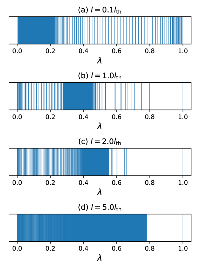
Figure 2: Graphical representation of the eigenvalue spectrum of the transition matrix ${\bm{\pi}}$ of the Markov chain for four different values of the $l/l_{\text{th}}$ ratio, for energy function (32), $k=1$. Another representation, which makes the degree of degeneracy more clear, is provided in Fig. 16. The matrix size is $1001\times 1001$.

Already the existing data suffice to highlight the qualitative changes in the eigen-value spectrum that accompany the diffusion-to-effusion crossover: Direct inspection of the eigenvalues indicates that as one approaches the crossover region coming from the diffusion limit $l\ll l_{\text{th}}$, the spectra clearly develop a gap separating $\lambda_{1}$ and $\lambda_{2}$, see Figs. 2 and 16. Note also that the 1D case analyzed above is the worst-case scenario in the sense that the optimal rate has the biggest value for one-dimensional simulations. Already in this worst-case scenario, the absolute value of the apparent rate $(1-\lambda_{2})\simeq 0.5$ is numerically close to the value $-\ln\lambda_{2}$ it would have, if we used the discrete prescription (16) for the wait times in place of the Poisson statistics. We provide values for both quantities $(1-\lambda_{2})$ and $-\ln\lambda_{2}$, respectively in Fig. 1, for the reader’s reference.

Conversely to the connections encapsulated in Eq. (44) and (45), we conclude that when multiple bound states with distributed sizes are present, one cannot calibrate parameter $\Delta t$ against an actual physical process. Despite this ambiguity, one still can, in principle, calibrate ratios of the relaxation rates for distinct bound states against actual systems, if it is known that the attempted step length $l$ is shorter than the size $l_{\text{th}}$ for every variety of bound state present. Suppose for the sake of argument that there are exactly two kinds of bound states, the respective thermal lengths given by $l_{\text{th}}^{(1)}$ and $l_{\text{th}}^{(2)}$. According to Eq. (33), the ratio of the corresponding sampling rates in the $l\to 0$ limit is given by

$$\frac{\tau^{(1)}}{\tau^{(2)}}=\left(\frac{l_{\text{th}}^{(2)}}{l_{\text{th}}^{(1)}}\right)^{2},\hskip 8.53581ptl\ll l_{\text{th}}^{(1)},l_{\text{th}}^{(2)}$$ (46)

independent of the value of $l$ and $\Delta t$. The quantity on the r.h.s. in the equation above is a geometric factor; it is also a ratio of two equilibrium properties. We see that although this ratio is, in principle, accessible to statistical sampling, the latter sampling must be suboptimal. For a valid comparison with actual systems, such systems must be overdamped.

III Classical Monte Carlo sequences are not physical trajectories, and ambiguities stemming from distribution of masses

Despite a causal relationship among the sampled configurations, sequences of coordinates generated in the course of Monte Carlo simulation do not correspond to snapshots of individual physical trajectories of inertial particles. Indeed, because of the absence of inertia intrinsic to Gibbs-sampling of a Boltzmann distribution, one is free to adopt a variety of probability distributions of waiting times $t$, including those distributions that are non-vanishing as $t\to 0$; the latter is the case for the Poisson statistics we employ here. An elementary calculation shows that under these circumstances, the distribution of the nominal rate of displacement $v_{\mbox{\tiny MC}}\equiv x/t$ has a long, inverse-quadratic tail:

$$p(v_{\mbox{\tiny MC}})\propto\frac{1}{v_{\mbox{\tiny MC}}^{2}},$$ (47)

and, hence, does not even have an average let alone higher moments. Thus, Monte Carlo “trajectories” are inherently discontinuous sequences of variables, while the displacement rate does not correspond to a velocity of an inertial particle, notwithstanding the kinematic-like relation (43) one may adopt under certain circumstances. Thus, even at optimal sampling—whereby statistical sampling of relaxations might effectively mimic physical motions—steps in classical Monte Carlo simulations can be, at best, thought of as ordered in terms of a pseudo-time. We demonstrate this more explicitly in what follows and, subsequently, begin discussing implications for quantifying activated dynamics when multiple bound states are present and masses of the bound modes are distributed.

To drive home the distinction between the Monte Carlo step and a physical time that can host inertial dynamics we consider a setup, in which both the MC step and a true dynamical time are explicitly present. First we recall that classical Monte Carlo simulations can be thought of as a way to compute the configurational part of the partition function of a system,

$$Z=\int dx\>e^{-\beta V(x)},$$ (48)

specifically using importance sampling. Newman and Barkema (1999) Here, $V(x)$ is the potential energy for the variable $x$. Next we consider, for the sake of argument, the configurational part of the partition function for an infinitely large set of equivalent replicas of a classical degree of freedom $x$ that is subject to a potential energy $V(x)$:

$$Z_{\text{r}}=\int dx\>Z(x,\beta)$$ (49)

where

$$Z(x,\beta) \equiv\lim_{N\to\infty}\int\left(\prod_{i=1}^{N-1}dx_{i}\right)$$

$$\times\exp\left\{-\sum_{i=1}^{N}\delta t\left[\frac{\kappa}{2}\frac{(x_{i}-x_{i-1})^{2}}{(\delta t)^{2}}+V(x_{i})\right]\right\}$$

$$=\int{\cal D}x\,\exp\left\{-\int_{-\beta/2}^{\beta/2}dt\left[\frac{\kappa\dot{x}^{2}}{2}+V(x)\right]\right\}$$ (50)

and $\delta t\equiv\beta/N$. Each replica is coupled to exactly two other replicas, thus allowing one to label these degrees of freedom using ordinals $i=1,\ldots,N$ while imposing periodic boundary conditions:

$$x_{0}=x_{N}\equiv x.$$ (51)

Thus the variables $x_{i}$, $i=1,\ldots,N$, are all formally equivalent, per Eq. (49). The replica-replica coupling constant, $\kappa/2(\delta t)^{2}$, is constructed so that the integral tends to a steady value in the limit $N\to\infty$. Indeed, expression (50) is formally equivalent to the diagonal entries of the (imaginary-time) density matrix for a quantum degree freedom $x$ of mass $m$ subject to a potential $V(x)$ Schulman (2012) where

$$\kappa\leftrightarrow\frac{m}{\hbar^{2}}.$$ (52)

In any event, we use the importance sampling of the integrand in Eq. (50) as a formal device to generate, in principle, continuous trajectories. Indeed, for each given value of its end-point, the sequence $\{x_{i}\}\leftrightarrow\{x(t)\}$ is a continuous function of the integration variable $t$ in the $N\to\infty$ limit. At the same time, an MC sequence for the end points (51) of a individual trajectory can have arbitrary increments, subject to the adopted proposal density. Next we stipulate that the Gibbs-sampling of the distribution defined by the integrand in Eq. (50) be optimal. This is equivalent to stipulating that we take the path integral along the steepest descent, so as to minimize the number of points where the integrand must be sampled. Further, the trajectory $x_{m}(t)$ that maximizes the integrand in Eq. (50):

$$\kappa\ddot{x}_{m}=-\partial(-V)/\partial x$$ (53)

happens to be the Newtonian trajectory of a particle with inertial mass $\kappa$ in the inverted potential $-V(x)$. Thus, the integration variable $t$ in Eq. (50) is a true dynamical time. The immediate vicinity of the optimum trajectory in the direction of steepest descent determines a multiplicative factor for the overall expression.

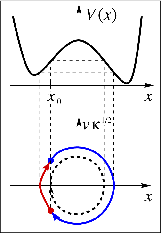
Figure 3: Sketches of two types of stationary trajectories for density matrix (50) for a bi-stable potential energy function: one trajectory is toward the adjacent bound state (thick red line), the other across the barrier separating distinct bound states (thick blue line). The thick dashed line shows the limiting shape of the latter curve when $\kappa\to\infty$.

The $\kappa\to\infty$ limit in Eq. (50) corresponds to the partition function sampled by classical Monte Carlo, by virtue of the formal correspondence (52). The result of taking this limit very much depends on the shape of the potential energy $V(x)$. Consider, for the sake of concreteness, a two-well potential and two distinct Newtonian trajectories—for the inverted potential $-V(x)$—each emanating from the same point $x_{0}$, but having opposite signs for the velocity $v\equiv dx/dt$, as in Fig. 3. We choose the point $x_{0}$ so that the curvature $\partial^{2}V/\partial x^{2}$ is positive at $x=x_{0}$, for concreteness. It will be convenient to visualize the trajectories in the plane $(x,v\sqrt{\kappa})$ (not the usual phase space $(x,\kappa v)$!). The initial points for the two trajectories are shown with dots. The two respective paths each have open ends, but smoothly complement each other to a cyclic path.

As one takes the $\kappa\to\infty$ limit, the Newtonian trajectory facing the adjacent bound state shrinks into a point at rates proportional to $1/\kappa$ and $1/\sqrt{\kappa}$ along the horizontal and vertical direction, respectively. Also, the magnitude of fluctuations around the classical path, along the $x$ direction, diminishes at a rate $\propto 1/\sqrt{\kappa}$ for large values of $\kappa$, in the usual fashion. Thus the path integral reduces to a sampling of just one variable, i.e, the position of the endpoint (51) itself when $\kappa\to\infty$, as is appropriate in the classical limit. The corresponding probability, up to the first non-vanishing term in $1/\kappa$ is given by the expression:

$$Z(x,\beta)\propto e^{-\beta[V(x)+(\beta\partial V/\partial x)^{2}/12\kappa]}$$ (54)

where the prefactor depends on the detailed form of the potential. For instance, for a parabolic bound state with a spring constant $k$, the prefactor is given by the normalization factor of the classical Boltzmann distribution $(\beta k/2\pi)^{1/2}$. Expression (54) clearly tends to a finite value as $\kappa\to\infty$.

In contrast, the trajectory crossing the transition state, which separates the two minima of $V(x)$, tends to a steady, cyclic shape in the $\kappa\to\infty$ limit. This limiting shape, shown by the thick dashed line in Fig. 3, corresponds to the cyclic Newtonian trajectory within the minimum of the inverted potential $-V(x)$ at energy $E=-V(x_{0})$ and represents an instanton. Coleman (1979) Thus in contrast with the trajectory facing the adjacent bound state, the path integral crossing the barrier corresponds to paths of finite length even in the $\kappa\to\infty$ limit. The corresponding value of the probability vanishes exponentially fast with $\kappa$ according to the following, WKB-like expression:

$$Z(x,\beta)\propto e^{-\beta V(x)}e^{-2\int dx\sqrt{2\kappa[V(x)-V(x_{0})]}}.$$ (55)

The vanishing of this expression in the $\kappa\to\infty$ limit means that the assumption of the ability of optimal Monte Carlo sampling to produce a continuous trajectory that connects two bound states and, thus, is guaranteed to sample the corresponding transition state is internally inconsistent. Conversely, optimal trajectories must avoid transition states. Furthermore, the optimal step length must be comparable to the distance between any two bound states implying the sampling will be effusive and not exhibit activation altogether. Instead, the sampling rate will reflect the volume of the thermally-populated region, as was argued in Section II.

When suboptimal, Monte Carlo sampling can be used to explore both bound states and transition states, of course, by making the typical step size small enough and, thus preventing bypassing of barriers. Still, in the absence of knowledge of the pertinent mass, there is no guarantee that the so detected bound states are actually present. Indeed, classical bound states in dimensions three and higher are, generally, not robust against quantum fluctuations. Schiff (1968) In spatial dimensions one and two, attractive potentials exhibit at least one bound state, see Ref. Chadan et al. (2003) and references therein. Still, the wavelength of the corresponding motion is determined by the Broglie wavelength corresponding to the depth $\epsilon$ of the bounding potential, i.e. $\lambda\simeq\hbar/\sqrt{m\epsilon}$, a quantity generally decoupled from the spatial extent of the bound state. (Note one does not expect to find modes with a strictly vanishing mass in dimensions one and two. Mermin and Wagner (1966); Hohenberg (1967); Coleman (1973)) In any event, one must separately decide whether the effective mass of a mode exhibiting vibrational relaxation during MC simulations is not so low as to lead an escape from the bound state by tunneling. For example, it seems plausible that classical MC simulations of water models might exhibit bound states that would be actually escaped by the light-weight proton.

When tunnening is significant, the actual motions will be qualitatively different from bound motions apparent to a classical simulation. For instance, imagine a two-well potential, each well representing a classical bound state. As tunneling becomes significant, with lowering the mass, a Larmor precession between the two minima becomes possible, if the interaction with the environment is not too strong. Wolynes (1981); Garg, Onuchic, and Ambegaokar (1985); Leggett et al. (1987) The frequency of the tunneling motion, then, sets a distinct, intrinsically quantum time scale. There is also the distinct possibility that the bound states would all melt cooperatively throughout the system, as would be the case during quantum melting of a solid. Schmalian and Wolynes (2000); Westfahl, Schmalian, and Wolynes (2003); Golden, Ho, and Lubchenko (2017); Lubchenko and Kurnosov (2019) The threshold amount of tunneling can be thought of as separating just two distinct phase behaviors that correspond to essentially classical and quantum behaviors, respectively. (We note that the survival, if any, of a bound state in the $m\to 0$ limit is analogous to the survival of a replica-symmetry broken state Mézard, Parisi, and Virasoro (1987); Rainone (2014) even as the replica-replica coupling vanishes.) The formation of bound states can be viewed as a pseudo-transition $(m=0)\to(m>0)$; the transition can be either continuous or discontinuous, by analogy with the metal-insulator transition. Golden, Ho, and Lubchenko (2017); Lubchenko and Kurnosov (2019) Bound states represent instances of broken translational symmetry. Thus one might view bound states and the pseudo-time $t/\sqrt{m}$ as emerging together as a result of lowering symmetry. In view of the slowness of the square root, one may view the robustness—or lack thereof—of Monte Carlo-produced relaxation functions, against the variation of mass among the modes, as a question of how far from the $(m=0)\to(m>0)$ transition the system is, if the transition is continuous. (Trouton’s law is an important example of a similar robustness, the latter stemming from the slowness of the logarithm. Lubchenko (2020)) When the transition happens to be discontinuous in the first place, one may view the ambiguity with respect to mass variation, among the modes, as quantitative, not qualitative. The more substantial source of ambiguity has to do with the presence of multiple length scales in problems of practical interest, as already stated, to be explicitly illustrated next.

IV Breaking of the pseudo-clock

Here we provide further evidence, using concrete model systems, that the apparent connection between the pseudo-time emerging in an MC simulation of a single-well bound state and physical timescales can not be exploited, in practice, to quantify the kinetics of activated transitions among distinct bound states. Such activated transitions often underlie a variety of chemical and/or transport phenomena of interest in applications. We shall call such activated processes “configurational” to distinguish them from equilibration within an individual free energy minimum and, also, in reference to distinct free energy minima usually corresponding to distinct microscopic configurations. Our first model system is a simple bi-stable potential energy surface

$$V(x)=\frac{k}{2}[(x/x_{0})^{2}-1]^{2}.$$ (56)

We fix the units by setting $x_{0}=1$ and $k=1$. The activation energy $E^{\ddagger}=k/2$ for configurational equilibration due to inter-well transitions is, thus, numerically equal to $1/2$. At sufficiently low temperatures, one expects the rate of configurational relaxation to become sufficiently lower than the rate of vibrational relaxation, thus giving rise to a time-scale separation between the two dynamical processes. To elucidate a potential connection, if any, of these actual dynamical processes with statistical sampling of the Boltzmann distribution corresponding to the potential energy (56), we perform Monte Carlo simulations for the latter potential energy using the move

$$x\to y\hskip 28.45274pt\text{(``move type 1'')}$$ (57)

where the value of the increment $(y-x)$ is distributed according to the proposal density $q(x,y)$ from Eq. (26), as before. We quantify the relaxation of the system by fitting the pair-correlation function

$$C_{xx}(t)\equiv\left\langle x(t)x(0)\right\rangle-\left\langle x\right\rangle^{2}$$ (58)

using a sum of exactly two exponential functions:

$$C_{xx}(t)=A_{v}e^{-t/\tau_{v}}+A_{c}e^{-t/\tau_{c}},\hskip 5.69054pt\tau_{v}<\tau_{c}$$ (59)

The labels “$v$” and “$c$” for the fitting parameters $\tau_{v}$ and $\tau_{c}$ anticipate that the “faster” process has to do with sampling an individual vibrational minimum while the “slower” process corresponds to sampling moves that traverse the maximum of the potential energy $V(x)$ or, equivalently, the minimum of the bi-modal Boltzmann distribution $p(x)\propto e^{-\beta V(x)}$.

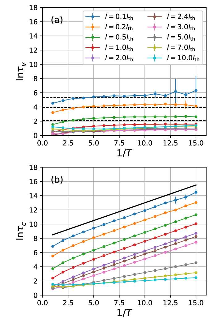
Figure 4: Arrhenius plots for the (a) shorter MC-relaxation time $\tau_{v}$ and (b) the longer MC-relaxation time $\tau_{c}$ for select values of the $l/l_{\text{th}}$ ratio obtained from two-exponential fits, Eq. (59), of the correlation functions (58) for energy function (56). $k=1$, $x_{0}=1$. In panel (a), the horizontal dashed lines show the value of the relaxation time evaluated using the short-$l$ asymptotics from Eq. (33) for $l/l_{\text{th}}=0.1$, $0.2$, $0.5$ top to bottom, respectively. In panel (b), the straight line corresponds to an activation dependence for a barrier strictly equal to $k/2$.

The Arrhenius plots for the quantities $\tau_{v}$ and $\tau_{c}$ are shown in Fig. 4(a) and (b), respectively. The configurational times are seen to follow rather closely the Arrhenius dependence for sufficiently low values of the step $l$, but not so for step sizes significantly greater than the size of an individual well, where the sampling is in the effusive regime, consistent with the discussion following Eq. (55). The prefactors for configurational relaxation times clearly correlate with the corresponding vibrational times. To quantify this correlation, we show the Arrhenius plot for the quantity $\tau_{c}e^{-E^{\ddagger}/k_{B}T}/\tau_{v}$ in Fig. 5. In the first place, the dimensionless ratio $\tau_{c}/\tau_{v}$ is worth plotting because it is independent of the “time” unit $\Delta t$ from Eq. (16), thus making it, essentially, a geometric quantity.

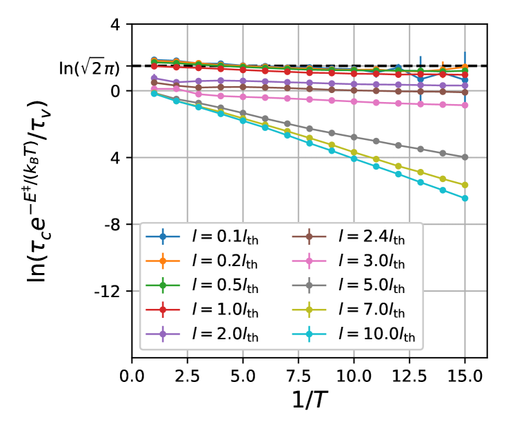
Figure 5: Arrhenius plots for the quantity $\tau_{c}e^{-E^{\ddagger}/k_{B}T}/\tau_{v}$ for the relaxation times from Fig. 4.

The data for $l/l_{\text{th}}\lesssim 1$ are seen to cluster around an activated dependence corresponding to the expected activation barrier $E^{\ddagger}=1/2$ and, furthermore, appear to tend to a fixed value at low temperatures. This behavior can be connected to some features of activated dynamics for actual molecular systems in the presence of strong damping. Indeed, we recall the simple approximation for the activation rate for escape from a bound state in the overdamped, Kramers limit discussed by Frauenfelder and Wolynes: Frauenfelder and Wolynes (1985)

$$k_{\text{escape}}=\left(\frac{2l_{\mbox{\scriptsize mfp}}}{l_{\mbox{\scriptsize TS}}}\right)\frac{\omega}{2\pi}e^{-E^{\ddagger}/k_{B}T}.$$ (60)

The quantity $\omega$ is the vibrational frequency of the bound state, while the $l_{\mbox{\scriptsize mfp}}/l_{\mbox{\scriptsize TS}}$ ratio on the r.h.s. reflects a reduction of the rate predicted by the transition state theory stemming from the mean free path $l_{\mbox{\scriptsize mfp}}$ being much smaller that the transition-state size $l_{\mbox{\scriptsize TS}}$. Frauenfelder and Wolynes (1985) The transition-state size is defined as the size of the region containing all points that are within $k_{B}T$ worth of energy from the barrier top. Frauenfelder and Wolynes (1985) The relaxation rate in a two-state system is equal to the sum of the two escape rates: $1/\tau_{c}=k_{1\to 2}+k_{2\to 1}$, which amounts to twice the escape rate from Eq. (60) in the present context. Thus one may use Eqs. (34) and (43) to obtain the following, very simple expression

$$\frac{\tau_{c}^{\text{(ph)}}e^{-E^{\ddagger}/k_{B}T}}{\tau_{v}^{\text{(ph)}}}=\frac{\pi}{2\sqrt{2}}\>\frac{l_{\mbox{\scriptsize TS}}}{l_{\text{th}}},$$ (61)

where we used the label “(ph)” to emphasize that the above equation pertains to a physical process. We see that in the overdamped limit, the quantity in Eq. (61) is not only geometric, as anticipated above, but is also expressed exclusively in terms of equilibrium quantities and, thus, might be accessible to thermodynamic sampling, c.f. the discussion following Eq. (46). In more detail, expression (61) is implicitly contingent on satisfying the constraints $l_{\mbox{\scriptsize mfp}}\ll l_{\mbox{\scriptsize TS}}$ and $\tau_{\mbox{\scriptsize auto}}\ll\tau_{v}^{\text{(ph)}}\ll\tau_{c}^{\text{(ph)}}$, but it does not explicitly contain either the mean free path $l_{\mbox{\scriptsize mfp}}$ or the autocorrelation time $\tau_{\mbox{\scriptsize auto}}$. At the same time, the Monte Carlo step size $l$ can be chosen to be smaller than the transition state size $l_{\mbox{\scriptsize TS}}$, while the wait time $\Delta t$ of the semi-Markov process, from Eq. (16), explicitly cancels out in the $\tau_{c}/\tau_{v}$ ratio, as already mentioned. Thus, whenever the MC times obey $\tau_{v}\ll\tau_{c}$ and the condition $l<l_{\mbox{\scriptsize TS}}$ is met, one should expect the geometric relation (61) to also hold for the relaxation profiles obtained in MC simulations, perhaps up to a factor of order 1, even though the MC times $\tau_{v}$ and $\tau_{c}$ cannot be individually connected to actual microscopic times. This is because expression (61) applies only when the actual dynamics is overdamped, see the discussion following Eq. (45).

Now, the barrier top of the energy (56) is an inverted parabola whose curvature $m(\omega^{*})^{2}$ is twice less than the curvature of the minima, hence $\omega^{*}=\omega/\sqrt{2}$. Since $l_{\mbox{\scriptsize TS}}=2^{3/2}(k_{B}T/m)^{1/2}$, Frauenfelder and Wolynes (1985), we obtain that $l\ll l_{\mbox{\scriptsize TS}}$ whenever $l\ll l_{\text{th}}$, and so the r.h.s. of Eq. (61) should tend to $\pi\sqrt{2}$ at low temperatures. This inference is quantitatively consistent with Fig. 5.

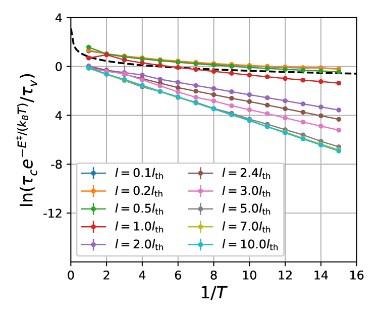
Figure 6: Arrhenius plots for the quantity $\tau_{c}e^{-E^{\ddagger}/k_{B}T}/\tau_{v}$ for the relaxation times for energy function (62). $k=1$, $x_{0}=1$. The dashed line gives the numerical value of the r.h.s. of Eq. (61).

Conversely, we can directly verify that when the condition $l<l_{\mbox{\scriptsize TS}}$ is not satisfied, results of Monte Carlo simulation do not strictly conform to Eq. (61). Indeed, consider for the sake of argument the following bi-stable energy function:

$$V(x)=\frac{k}{2}(x^{2}-x_{0}|x|),$$ (62)

whereby the two minima are strictly parabolic while the barrier is a cusp formed by two straight lines with slopes $\pm kx_{0}$. The resulting data for the $\tau_{c}e^{-E^{\ddagger}/k_{B}T}/\tau_{v}$ ratio are shown in Fig. 6. For this form of the potential, the transition state size scales linearly with temperature $l_{\mbox{\scriptsize TS}}=2(k_{B}T/kx_{0})$, Frauenfelder and Wolynes (1985) and can become arbitrarily shorter than the thermal length $l_{\text{th}}=\sqrt{k_{B}T/k}$. In any event, the Kramers limit for actual dynamics would now yield $\pi\sqrt{k_{B}T/k}/x_{0}$ for the r.h.s. of Eq. (61). Though this estimate falls in the ballpark for the Monte Carlo-generated data in the low $l/l_{\text{th}}$ regime, we see that the simulation consistently underestimates the activation barrier. This is expected because when $l>l_{\mbox{\scriptsize TS}}$, crossing of the barrier is no longer conditional on sampling the barrier top thus effectively leading to the barrier being bypassed, the extent of bypassing depending on the value of $l/l_{\mbox{\scriptsize TS}}$.

The main message conveyed by Figs. 5 and 6 is this: There is no reliable way to associate a pseudo-time with activated relaxations observed in the course of Monte Carlo simulations, unless the $l/l_{\text{th}}$ ratio is small and the barrier top is smooth. Even so, such a small step size corresponds to a diffusive sampling regime and is computationally inefficient.

We next elaborate on the preceding discussion of barrier bypassing. To this end, we use an artificial energy function where the rate of barrier-bypassing moves and the degree of bypassing can be rigidly controlled. Indeed, consider the following simple energy function:

$$V(x,\sigma)=-(kx_{0})x\sigma+\frac{kx^{2}}{2}$$ (63)

where $x$ is a continuous degree of freedom while the quantity $\sigma$ is an Ising spin-like degree of freedom that is allowed to have only two values: $\sigma=\pm 1$. It is easy to see that the effective free energy for the variable $x$:

$$F(x) =-k_{B}T\ln\left[\sum_{\sigma=\pm 1}e^{-\beta V(x,\sigma)}\right]$$

$$=-k_{B}T\ln\left[2\cosh(\beta kx_{0}x)\right]+\frac{kx^{2}}{2}$$ (64)

becomes bistable below the temperature $T_{0}=kx_{0}^{2}/k_{B}$, the two minima corresponding to the vibrational ground states $x=\pm x_{0}$, which in turn pertain to the two distinct values of the spin $\sigma=\pm 1$, respectively. Thus one is able to unambiguously distinguish the two alternative vibrational ground states of the system, despite the barrier separating the two minima on the free energy surface (IV) being finite. Note the $T\to 0$ limit of the free energy $F(x)$ yields energy function (62), up to an additive constant. Energy function (63) can be viewed as a classical limit of the problem of non-adiabatic transport of a particle interacting with a harmonic environment, Kubo and Toyozawa (1955); Ovchinnikov and Ovchinnikova (1982); Marcus (1964) whereby the two terms corresponding to $\sigma=\pm 1$, respectively, are the usual Marcus parabolas.

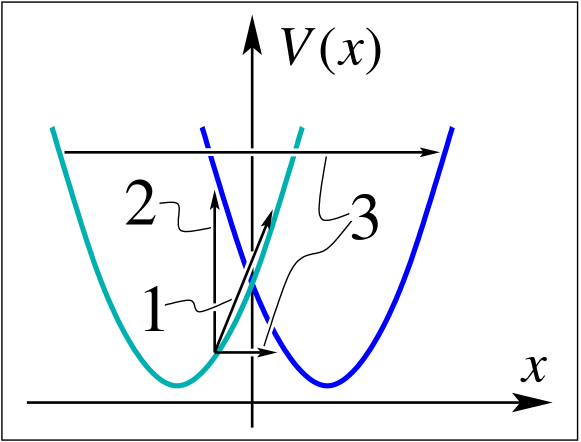
Figure 7: Monte Carlo moves of the three types employed in the present work, Eqs. (57), (65), and (66) and the respective energy changes are graphically illustrated by straight arrows.

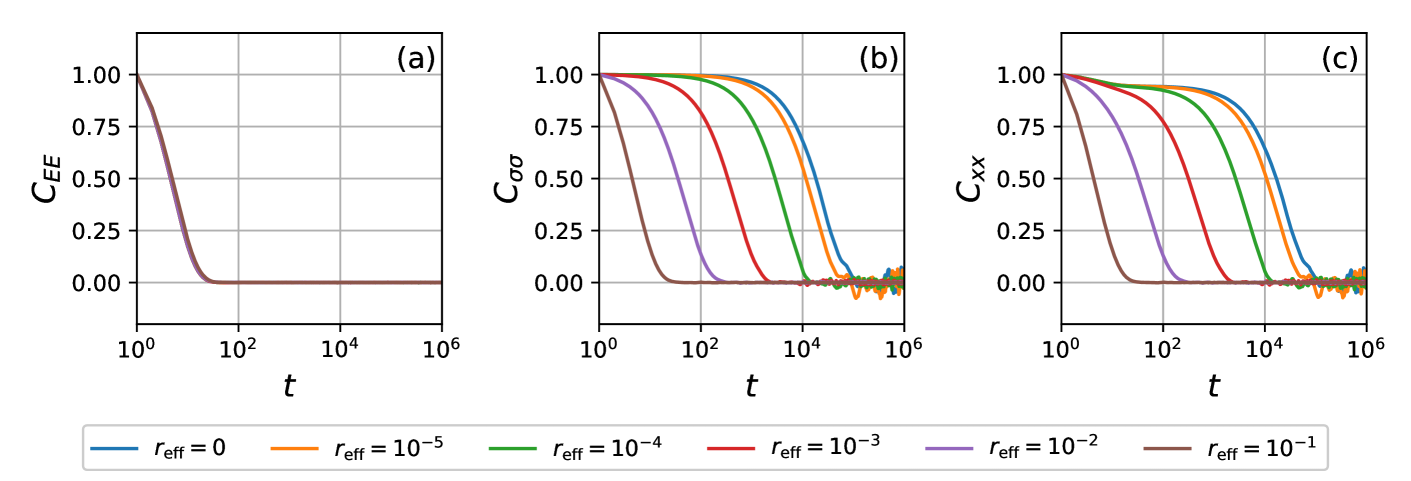
Figure 8: Relaxation profiles for equilibrium Monte-Carlo simulations of energy function (63). $T=0.07$, $k=1$, $l/l_{\text{th}}=2.38$, $r=1$. Panels (a), (b), and (c), show the correlation functions from Eqs. (67), (68), and (58), respectively.

We will continue using moves of type 1 from Eq. (57) to sample the individual vibrational terms. To enable transitions between the latter terms, we will use a combination of two types of move: One is the simple spin-flip move:

$$\sigma\to-\sigma\hskip 28.45274pt\text{(``move type 2'')}$$ (65)

Already moves of type 1 and 2, together, allow one to fully sample the phase space of the system. By construction, we denote the number of attempts for move 2, relative to move 1, with letter $r$. We directly illustrate in Fig. 7 that the energy cost to transition between the two vibrational ground states is bounded from below by the barrier height $E^{\ddagger}=k/2$, if only moves of type 1 and 2 are used.

The other move type that will be used to switch between the vibrational terms involves both variables at the same time:

$$x\to-x,\>\>\sigma\to-\sigma\hskip 28.45274pt\text{(``move type 3'')}$$ (66)

This move is isoenergetic and, thus, bypasses the classical barrier separating the two minima of the energy function, if the initial energy is below the crossing point of the two Marcus parabolas, see Fig. 7. A combination of moves of type 1 and 3 is fully ergodic. We will denote the rate of these “non-physical” moves, relative to the rate of moves of type 1, with $r_{\text{eff}}$, in reference to these moves being strictly effusive.

In Fig. 8, we display the following pairwise correlation functions:

$$C_{EE}(t) \equiv\left\langle E(t)E(0)\right\rangle-\left\langle E\right\rangle^{2}$$ (67)

$$C_{\sigma\sigma}(t) \equiv\left\langle\sigma(t)\sigma(0)\right\rangle-\left\langle\sigma\right\rangle^{2}$$ (68)

as well as the correlation function (58). Data in Fig. 8 cover a broad range of the attempt rate $r_{\text{eff}}$ for the non-physical move.

We observe that the energy-energy correlation function relaxes much faster than the other two correlation functions. This is because the two vibrational ground states are degenerate and so the value of energy is not sensitive to the precise identity of the minimum. In contrast, the spin-spin correlation function does not reach its long-term value until the configurational equilibration has occurred. Already above a certain, very low rate of the non-physical move of type 3, the kinetics of configurational relaxation are dominated by the latter non-physical process. Furthermore, above a certain value of $r_{\text{eff}}$, the overall relaxation cannot be identified with either vibrational or activated processes and is completely slaved to the effusive move. We also observe that in addition to short-circuiting the activation barrier, the non-physical move modifies the vibrational relaxation, too.

From here on, we focus on the activated dynamics and set $r_{\text{eff}}=0$ until further notice. Both the vibrational and configurational contributions are clearly seen in the $x-x$ correlation function, whereby the configurational contribution shows up as a pronounced plateau. The vertical position of the plateau is a Debye-Waller factor. Lowering of this position, relative to unity, is approximately given by the $l_{\text{th}}/x_{0}$ ratio, of course. Note that the spin-relaxation profile also has a shorter-term, vibrational contribution, but the latter contribution is determined by the staggered susceptibility of the spin, $\simeq 1/\cosh^{2}(\beta kx_{0}^{2})$, and is too small numerically to be seen on the graph, at the temperature in question.

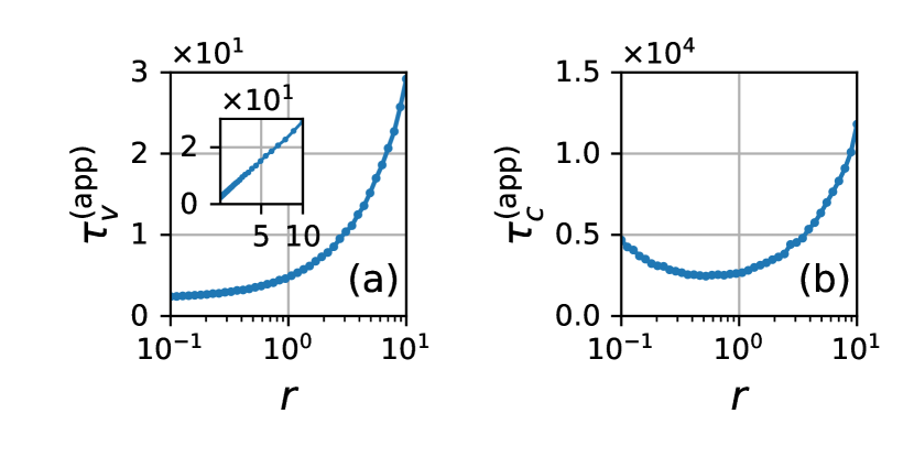
Figure 9: Apparent relaxation times determined by fitting the time traces of the $C_{xx}$ from Eq. (58), using the two-exponential form from Eq. (59), as functions of the ratio $r$ of the attempt rates for the configurational and vibrational degree of freedom. Panels (a) and (b) show the shorter time $\tau_{v}$ and longer time $\tau_{c}$, respectively. The energy function is from Eq. (63). $T=0.1$, $k=1$, $l/l_{\text{th}}=2.38$.

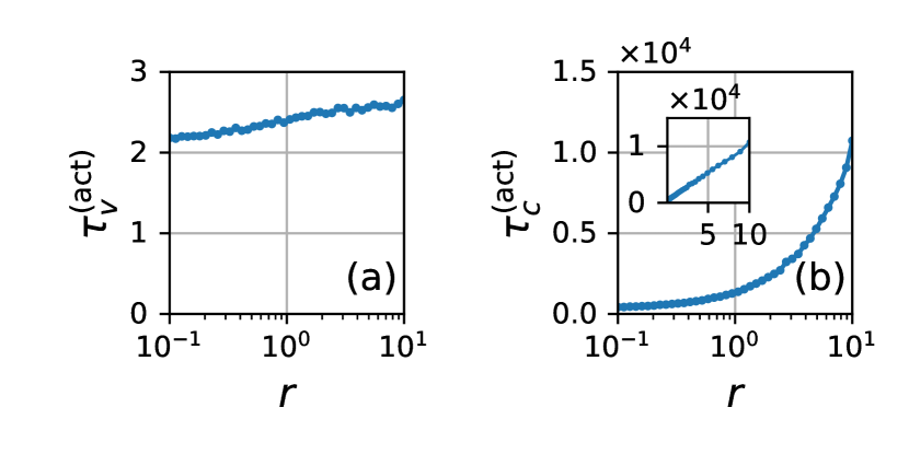
Figure 10: Relaxation times from Fig. 9 rescaled according to Eqs. (69) (panel a) and (70) (panel b), respectively, so as to that account for the variation of the attempt rate $r$.

In Fig. 9, we show the $r$ dependence of the apparent relaxation times $\tau^{\text{(app)}}_{v}$ and $\tau^{\text{(app)}}_{c}$ for the vibrational and configurational relaxation, respectively, as inferred directly from the relaxation profiles. The near linear increase of $\tau^{\text{(app)}}_{v}$ with the attempt ratio $r$, seen in Fig. 9, occurs because for greater values of $r$, a progressively larger fraction of attempts is spent on the spin flip, and vice versa for $\tau^{\text{(app)}}_{c}$. Thus in Fig. 10, we graph the relaxation times suitably adjusted to accommodate for this circumstance:

$$\tau^{\text{(act)}}_{v} =\tau^{\text{(app)}}_{v}\frac{1}{1+r}$$ (69)

$$\tau^{\text{(act)}}_{c} =\tau^{\text{(app)}}_{c}\frac{r}{1+r}$$ (70)

We observe that the rescaled vibrational times now vary only modestly within a substantial range of $r$. At the same time the rescaled configurational time varies about as much as the apparent time $\tau^{\text{(app)}}_{c}$. In any event, both $\tau^{\text{(act)}}_{v}$ and $\tau^{\text{(act)}}_{c}$ are seen to increase monotonically with $r$. We observe that even when the number of control parameters for the simulation is the same as the number of distinct relaxation times, the latter relaxation times cannot be optimized simultaneously. This notion is consistent with the discussion following Eq. (55).

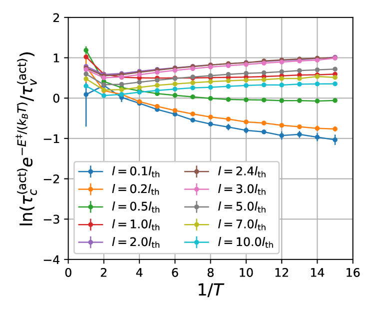
Figure 11: Arrhenius plots for the quantity $\tau_{c}e^{-E^{\ddagger}/k_{B}T}/\tau_{v}$ for the relaxation times observed during Gibbs-sampling energy function (63). The times are rescaled to account for the variation of the attempt rate $r$, as in Fig. 10. $k=1$, $r=0.5$. A straight line with a vanishing slope would correspond to strict activation at $E^{\ddagger}=k/2=1.2$.

Next we show in Fig. 11 the simulated value for the quantity $\tau_{c}e^{-E^{\ddagger}/k_{B}T}/\tau_{v}$ for the energy function (63). Here we observe that in contrast with the bi-stable potential energy functions analyzed earlier, the quantity $\tau_{c}e^{-E^{\ddagger}/k_{B}T}/\tau_{v}$ now depends on the $l/l_{\text{th}}$ ratio in a decidedly non-monotonic fashion. This behavior stems from the recurrent dependence of the relaxation time within an individual bound state. The configurational relaxation time also follows this trend, see Fig. 12, but to a lesser degree. In any event, we observe that for all values of the $l/l_{\text{th}}$ ratio, the data in Fig. 11 correspond to a lack of strict activation, within the temperature range of the simulation. A strict Arrhenius dependence does appear to set in at lower temperature, at the expected value of the activation barrier $E^{\ddagger}=1/2$, consistent with the lack of barrier-bypassing when $r_{\text{eff}}=0$.

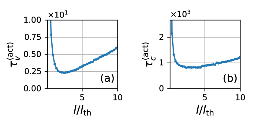
Figure 12: Rescaled relaxation times from Eqs. (69) (panel a) and (70) (panel b) as functions of the step length $l$. $k=0.1$, $r=0.5$.

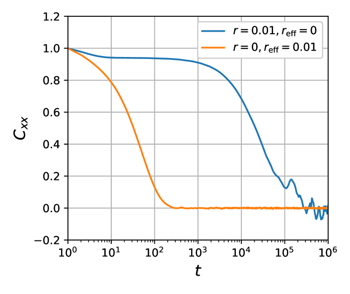
Figure 13: Select relaxation profiles for equilibrium Monte-Carlo simulations of energy function (63) for the “physical” and “non-physical” protocols, respectively, as pertinent to Figs. 14 and 15. $T=0.1$, $k=1$, $l/l_{\text{th}}=2.38$.

In the remainder of this Section, we consider effects of using barrier-bypassing moves on the quality of sampling of the free energy surface. We focus on two distinct simulation protocols, both ergodic. Protocol 1, call it the “physical” protocol, uses only moves of type 1 and 2, whereby bypassing of the barrier is strictly forbidden. Protocol 2, call it the “non-physical” protocol, uses only moves of type 1 and 3. Equilibrium relaxation profiles, as well as the pertinent parameters are provided in Fig. 13 and its caption. We choose the attempt rate of move 3 so that the corresponding relaxation is much faster than that in protocol 1, but still takes a substantial number of Monte Carlo steps, i.e., 50 or so.

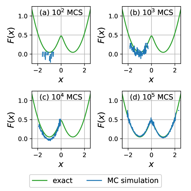
Figure 14: Histogram of the values of the coordinate $x$ for four select values of the collection time, for the “physical” protocol, move types 1 and 2, energy function from Eq. (63), same conditions as in Fig. 13. The solid line is the equilibrium free energy as a function of $x$, from Eq. (IV).

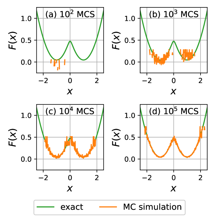
Figure 15: Histogram of the values of the coordinate $x$ for four select values of the collection time, for the “non-physical” protocol, move types 1 and 3, energy function from Eq. (63), same conditions as in Fig. 13. The solid line is the equilibrium free energy as a function of $x$, from Eq. (IV).

In Figs. 14 and 15, we histogram the values of the coordinate $x$ that we collect starting in some equilibrated configuration. We present results for four select values of the collection time, where we normalize the histograms and compute the corresponding free energy by taking the logarithm and multiplying by $(-k_{B}T)$. We observe that for the physical protocol, both free energy minima become adequately sampled on times comparable to the typical relaxation time. The transition-state region will have been sampled by that point as well. These results can be contrasted with those obtained using the non-physical protocol, see Fig. 15: When the collection times exceed the relaxation time by an order of magnitude or so, both minima have been securely sampled, but not the transition state. The latter only becomes adequately sampled, at least by visual inspection, on times that are at least two orders of magnitude greater than the relaxation time.

To rephrase these notions from the viewpoint of computational efficiency, the non-physical protocol offers an improvement in the efficiency of thermodynamic sampling by about two orders of magnitude, but it is achieved at the expense of avoiding transition state configurations, which are relatively high in free energy. While employment of the non-physical move does seem to speed up the sampling of the transition-state configurations, the improvement is only modest, an order of magnitude or so. Most importantly, the timescale on which the transition state becomes adequately sampled exceeds the apparent relaxation time by at least two orders of magnitude. We expect these trends to be general, the quality of transition state sampling becoming progressively poorer for higher barriers. Such accelerated simulations are unlikely to generate the bottle-neck configurations on which the transport is conditional, thus preventing one from establishing the mechanism of the activated transitions. This is, of course, consistent with the absence of slow processes, in the simulated relaxation profiles, that one associates with activation in the first place.

V Brief summary and implications for simulations of glassy mixtures

We have shown that notwithstanding its ability to efficiently sample the thermodynamics of a classical system, Gibbs sampling of the Boltzmann distribution cannot be used to reliably quantify the kinetics of relaxation toward equilibrium. Because Gibbs sampling lacks an inherent time scale, one cannot unambiguously assign a time scale to the semi-Markov process associated with the sampling, if the original physical system exhibits a distribution of relaxation rates.

The argument started out by considering the special case when the physical motion is confined to a single-well bound state in equilibrium with its environment. When not overly damped, this motion can be mimicked by a semi-Markov process, if the sampling is optimal. This setup is rather peculiar and seems to pertain to mechanically stable arrangements of hard objects. Hereby the relaxation rate of MC simulation can be unambiguously connected with the actual relaxation rate and frequency of the vibrational motion within the bound state, via a universal relation. Also at optimal sampling, the transition matrix of the Markov chain corresponding to the Metropolis sampling develops a well defined gap between the two largest eigenvalues. One may thus define a pseudo-clock, which can be thought of as emerging together with the underlying bound state and thus requires symmetry breaking. In this way the pseudo-clock is similar to actual clocks based on cyclic processes, since such cyclic motions also require symmetry breaking to occur so as to confine the motion. Furthemore, when the clock is based on a quantum process, the corresponding frequency is directly related to a gap in the spectrum as is the pseudo relaxation time.

In all other cases, the pseudo-clock breaks down. For instance, MC simulations of uniform liquids, which are translationally invariant, cannot be calibrated against actual systems. When two or more bound states are present, a number of distinct relaxation processes will take place. Since it is impossible to optimize the step size for all processes at the same time, the dynamics for the compound process will be rendered incorrectly. Of particular interest is the interplay of activated relaxation among distinct bound states and the vibrational relaxation within in an individual bound state. We have shown explicitly that vibrational relaxation—as apparent in MC simulations—cannot be reliably used as a reference time scale for activated reconfigurations among the bound states. This is particularly evident in the effusive regime of sampling, whereby the step size can be made so large as to cover more than one bound state. Hereby, transitions among distinct bound states do not require activation because the corresponding barriers are bypassed. Such effusive moves restore the symmetry while the relaxation time is determined by the volume of the thermally accessible regions, not the height of the barrier separating the bound states. Making the step size small allows one to recover a time-scale separation between vibrational and configurational equilibration, as well as the height of the activation barrier, but at the cost of making the simulation diffusive in nature and, thus, impractically slow. In any event, the values of the rates of configurational and vibrational relaxation alike can not be individually connected with actual physical processes.

According to the present findings, accelerated Monte Carlo protocols that make thermodynamic sampling more efficient do so at the expense of avoiding the bottle-neck configurations corresponding to the transition states for activated transport thus precluding one from detecting the latter configurations.

The latter notion has implications for simulational studies of glassy liquids; some of these studies were mentioned in the Introduction. According to the RFOT theory, Kirkpatrick, Thirumalai, and Wolynes (1989); Lubchenko and Wolynes (2007); Lubchenko (2015) molecular transport in glassy liquids and frozen glasses is slow because the translational symmetry characteristic of uniform liquids is transiently broken on times shorter than the lifetimes of metastable aperiodic structures that form below a dynamic crossover. Transport in such liquids requires activated escape from those metastable configurations and, thus, is subject to bottle-neck, transition-state configurations, in which a relatively large number of particles, call it $N^{\ddagger}$, must reconfigure. Lubchenko and Wolynes (2004); Lubchenko and Rabochiy (2014) The quantity $N^{\ddagger}$ grows as temperature is lowered, implying activated transport in glassy liquids should become increasingly more cooperative alongside. In quantitative terms, the cooperativity scale $N^{\ddagger}$ grows to about 50 rigid molecular units near the laboratory glass transition on the hour time scale. Xia and Wolynes (2000); Rabochiy, Wolynes, and Lubchenko (2013); Lubchenko and Rabochiy (2014) Once the the bottle-neck configuration is overcome, the transition will proceed to span a relatively compact region of size $N^{*}\simeq 4N^{\ddagger}$. Xia and Wolynes (2000); Eastwood and Wolynes (2002); Lubchenko (2018) Glassy liquids are predicted to exhibit inherent built-in stress Bevzenko and Lubchenko (2009, 2014) that varies spatially on the length scale $(N^{*})^{1/3}$; it is however not clear whether there should be an explicit spatial signature to this variation of stress. Even so, it was argued in Refs. Zhugayevych and Lubchenko (2010a, b); Lukyanov, Golden, and Lubchenko (2018) that in materials exhibiting charge-density waves, the strained regions exhibit a quantum-mechanical signature in the form of midgap electronic states.

According to the present results, accelerated Monte Carlo protocols that avoid bottle-neck configurations for activated transport cannot be used to quantify the extent of cooperativity during the activated events. We have devised a caricature model that has common features with particle-swap simulations. In both cases, two degrees of freedom undergo large, effusive displacements at the same time, a non-physical move that can be used to dramatically speed up thermodynamic sampling of typical states. We have seen that the deeper in the free energy landscape the accelerated simulation can equilibrate, the less likely is one to detect transition-state configurations. Considering that effusion is a phenomenon pertinent to dilute gases, barrier-bypassing moves—when used to simulate a glassy liquid—can be thought of as the liquid boiling locally! Such processes are clearly physically irrelevant at densities in question. We have also seen that such effusive processes can modify properties of the bound states and can even effectively destroy them.

Conversely, the present results indicate that to quantify the cooperativity and kinetics of activated reconfigurations in a glassy liquid, one must impose a sense of continuity to the trajectories at least to some extent. This can be done by (numerically) solving Newton’s equations of motion, of course. Alternatively, one can employ Monte Carlo simulations in the diffusive regime, as already mentioned, or by simulating multiple, coupled replicas of the system, per the discussion in Section III. In all of those cases, however, the respective protocols are computationally expensive. The notion of replicating the system—with the aim of elucidating activated transport—should not be too surprising, since replica methodologies can be used to detect breaking of translational symmetry in aperiodic systems that do not have an obvious structural-reference state. Monasson (1995); Rainone (2014)

Likewise, the present results are consistent with a notion that hydrodynamic, coarse-grained descriptions of the glass transition, such as the mode-mode coupling theory, Götze (2008) (MCT) do not apply below the dynamic crossover. Indeed, such coarse-graining implies that system can bypass the reconfiguration barriers thus leading to a description that effectively operates on a single free energy minimum. In contrast, the number of the latter minima scales exponentially with the system size and becomes huge already for modestly-sized samples, a fact that can be directly confirmed using calorimetry. Lubchenko (2015)

Acknowledgments

We thank Eric Bittner for sharing his expertise. We gratefully acknowledge the support by the NSF Grants CHE-1465125 and CHE-1956389, the Welch Foundation Grant E-1765, and a grant from the Texas Center for Superconductivity at the University of Houston. We gratefully acknowledge the use of the Maxwell/Opuntia Cluster at the University of Houston. Partial support for this work was provided by resources of the uHPC cluster managed by the University of Houston and acquired through NSF Award Number ACI-1531814. This article is dedicated to the memory of Hans Frauenfelder.

Appendix A General expression for the relaxation profile of an eigenvector of the transition matrix for an arbitrary distribution of wait times

The following discussion heavily relies on standard results from renewal theory, Ross (1992) however is intended to be reasonably self-contained. Everywhere below, the quantity $t$ stands for the time variable of semi-Markov processes, not a physical time. Suppose the initial condition ${\bm{p}}(t=0)$ for the Markov chain is given by a non-stationary eigenvector of the transition matrix ${\bm{\pi}}$ whose eigenvalue is $\lambda<1$. Following each Monte Carlo event, the transition matrix is applied to the current value ${\bm{p}}(t)$. $n$ such applications to the initial distribution results in scaling it down by an overall factor $\lambda^{n}$. By time $t$, an arbitrary number of Monte Carlo can occur, in principle, depending on the detailed form of the waiting-time distribution $\psi(t)$. Here we ask: What is the expectation value for the scaling factor $p_{\lambda}(t)$, at time $t$? By construction:

$${\bm{p}}(t)=p_{\lambda}(t){\bm{p}}(t=0).$$ (71)

We determine this expectation value $p_{\lambda}(t)$ by averaging $\lambda^{n}$ over the probability $P_{n}(t)$ that exactly $n$ Monte Carlo events occurred by time $t$:

$$p_{\lambda}(t)=\sum_{n=0}^{\infty}\lambda^{n}P_{n}(t).$$ (72)

Consider, for instance, the Poisson process with relaxation time $\Delta t$: $P_{n}(t)=e^{-t/\Delta t}(t/\Delta t)^{n}/(n!)$. In the latter case, Eq. (72) immediately yields $p_{\lambda}(t)=e^{-(1-\lambda)t/\Delta t}$, consistent with Eq. (19). Generally,

$$P_{n}(t)=F_{n}(t)-F_{n+1}(t),$$ (73)

where $F_{n}(t)$ is the (cumulative) probability that the $n$-th renewal has occurred by time $t$ or, equivalently, that the number of renewals by time $t$ is greater than or equal to $n$. By construction, the survival probability of the renewal process is the probability that no renewal has occurred:

$$P_{0}(t)=1-F_{1}(t)=1-\int_{0}^{t}\psi(t)\>dt$$ (74)

and we avoid pathological cases by adopting

$$F_{n}(0)=0.$$ (75)

The probabilities $F_{n}(t)$ are connected through an iterative relation:

$$F_{n+1}(t) =\int_{t_{n}+t_{1}<t}dF_{n}(t_{n})\>dF_{1}(t_{1})$$ (76)

$$=\int_{0}^{t}F_{n}(t-t_{1})\>dF_{1}(t_{1}),$$ (77)

which, we see, happens to be a convolution. Taking the Laplace transform and using the second equality in Eq. (74), as well as Eq. (75), readily yields:

$$\widetilde{F}_{n}(s)=\frac{1}{s}\,\widetilde{\psi}^{n}(s).$$ (78)

Computing the Laplace transform of Eq. (72), while using Eq. (73), becomes a matter of summing a geometric series, which, then, yields Eq. (20) of the main text.

Appendix B Diffusion-to-effusion crossover: Auxiliary information

First we obtain an approximation for the Monte Carlo sampling rate in the large $l$ limit of Eq. (II) for the one-dimensional case. We do not have in our possession the functional form of eigenvectors pertaining to the largest non-stationary eigenvalue $\lambda$ of the transition matrix. Instead, we consider a simple trial form that is linearly independent from the stationary solution of master equation (II), $\widetilde{p}=\text{const}$, and whose symmetry with respect to reflection about the origin is consistent with the energy function (32). Specifically we consider a solution that is odd and has its single node located at the origin—while being constant on the positive and negative side of the vertical axis, respectively:

$$p(x,t)=A(t)\,\text{sign}(x)$$ (79)

With the aid of this ansatz, proposal density (26) and energy function (32) yield for $x<0$:

$$(\Delta t)\frac{-\dot{A}}{2A}=\int_{0}^{|x|}dy\,q(x,y)+\int_{|x|}^{\infty}dy\,e^{-(y^{2}-x^{2})/2l_{\text{th}}^{2}}\>q(x,y)$$ (80)

Since the r.h.s. of this equation varies with $x$, the ansatz from Eq. (79) is internally-inconsistent, the degree of inconsistency dependent on the value of $x$. Still, Eq. (80) can thought of, informally, as providing the relaxation rate as a function of the coordinate. Averaging both sides of the equation with respect to the equilibrium distribution of $x$ will single out the most relevant values of the coordinate. Thus, we multiply by $2e^{-x^{2}/2l_{\text{th}}^{2}}/(2\pi l_{\text{th}}^{2})^{1/2}$ and integrate over the negative $x$’s:

$$-\frac{\dot{A}}{A}=\frac{4}{\Delta t}\int_{-\infty}^{0}\frac{dx}{\sqrt{2\pi l_{\text{th}}^{2}}}\left[e^{-x^{2}/2l_{\text{th}}^{2}}\int_{0}^{|x|}dy\>q(x,y)\right.$$

$$+\left.\int_{|x|}^{\infty}dy\,e^{-y^{2}/2l_{\text{th}}^{2}}\>q(x,y)\right]$$ (81)

In the limit $l_{\text{th}}\ll l$, one can ignore the variation of the function $q(x,y)$ in both integrals over $y$: $q(x,y)\approx 1/\sqrt{2\pi l^{2}}$. Thus, the first integral is well approximated by $|x|/\sqrt{2\pi l^{2}}$. The second integral will be approximated by the expression $e^{-x^{2}/2l_{\text{th}}^{2}}(l_{\text{th}}/2l)$, which is viewed as a compromise between the small-$x$ power-law expansion and the large-$x$, asymptotic expansion of the error function. (The resulting error, if any, becomes less significant in higher dimensions, where this term is subdominant, see below.) This immediately gives:

$$-\frac{\dot{A}}{A}(\Delta t)\approx\left(\frac{2}{\pi}+1\right)\frac{l_{\text{th}}}{l}\approx\frac{1}{0.61}\>\frac{l_{\text{th}}}{l}.$$ (82)

Higher-dimensional cases can be considered analogously, by making the function $p$ odd along exactly one spatial direction. This yields

$$-\frac{\dot{A}}{A}(\Delta t)\approx\left[\frac{2}{d}\>\frac{\Gamma(d)}{\Gamma^{2}(d/2)}+1\right]\left(\frac{l_{\text{th}}}{l}\right)^{d}\equiv f_{d}\left(\frac{l_{\text{th}}}{l}\right)^{d},$$ (83)

where $\Gamma$ is the standard gamma function. Abramowitz and Stegun (1964)

We next introduce a simple interpolative expression for the $(l/l_{\text{th}})$-dependence of the sampling rate that is consistent with both the small and the large $l$ asymptotics, Eqs. (33) and (83) respectively, as well as the $d\to\infty$ scaling of the optimal value of $l$.

$$\frac{\Delta t}{\tau}\simeq\frac{1}{2}\frac{(l/l_{\text{th}})^{2}}{[n_{d}(l/l_{\text{th}})^{2}+1]^{d/2+1}}.$$ (84)

where

$$n_{d}\equiv(2f_{d})^{-2/(d+2)}$$ (85)

and $f_{d}$ is defined in Eq. (83).

Eq. (84) readily yields for the optimal step size:

$$\frac{l_{\text{opt}}}{l_{\text{th}}}=\frac{1}{\sqrt{d}}\>\left[2^{1/2}(2f_{d})^{1/(d+2)}\right]\equiv\frac{C_{1}(d)}{d^{1/2}}\xrightarrow[d\to\infty]{}\frac{2^{3/2}}{\sqrt{d}}$$ (86)

The quantity in the square brackets, which we denote with $C_{1}(d)$, is a slow-varying function of $d$ that is limited from below by 2 or so and becomes a monotonically increasing function of $d$ for large values of the latter variable. $C_{1}(d)$ tends to $2\sqrt{2}\approx 2.8$ as $d\to\infty$. This is about 15% greater than the value reported in Ref. Roberts and Rosenthal (2001). At $d=1$, we have $\approx 2.1$, i.e., about 20% below the (numerically) exact value obtained in the simulation, see Fig. 1. Thus the closed-form expression (84), while approximate, provides satisfactory accuracy while preserving the essential scaling with $d$.

The value of the optimal rate itself

$$\frac{\Delta t}{\tau_{\text{opt}}}=\frac{1}{d}\>\frac{(2f_{d})^{2/(d+2)}}{(2/d+1)^{d/2+1}}\equiv\frac{C_{2}(d)}{d}\xrightarrow[d\to\infty]{}\frac{4/e}{d}$$ (87)

is evaluated near the stationary region of the actual function (whose exact value we do not possess) and, thus, is less sensitive to the details of the approximation. It gives $\tau_{\text{opt}}/\Delta t\approx 2.4$ in 1D, in good agreement with Fig. 1, as well as yielding the correct $d\to\infty$ scaling. The multiplicative factor $4/e\approx 1.47$ is about 10% off the estimate $2.38^{2}\times 0.234\approx 1.32$ reported in Ref. Roberts and Rosenthal (2001).

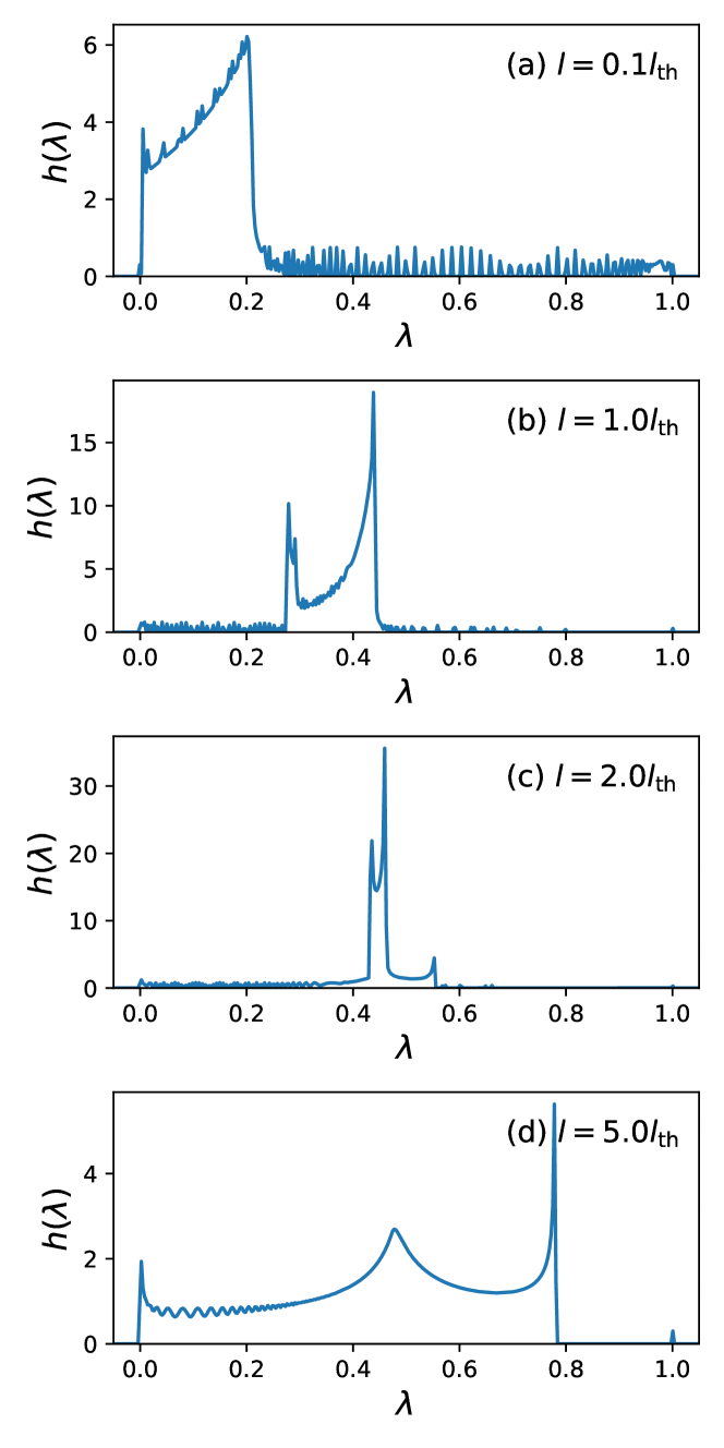
Figure 16: The spectrum of the transition matrix $\pi$ of the Markov chain for four select values of the $l/l_{\text{th}}$ ratio. Each energy level is represented by a narrow (width=0.001) Gaussian peak of unit area. $1001\times 1001$.

Finally, in Fig. 16, we show a coarse-grained spectrum of the eigen-values $\lambda$ of the transition matrix ${\bm{\pi}}$ corresponding to the parabolic energy function (32), so as to complement Fig. 2. The coarse-graining is performed by centering a narrow Gaussian peak at each individual value of $\lambda$. Note the large-$\lambda$ end of the spectrum is difficult to see. For this end of the spectrum, please consult Fig. 2.

References

- Newman and Barkema (1999) M. Newman and G. Barkema, Monte Carlo Methods in Statistical Physics (Clarendon Press, 1999).
- Socci, Onuchic, and Wolynes (1996) N. D. Socci, J. N. Onuchic, and P. G. Wolynes, “Diffusive dynamics of the reaction coordinate for protein folding funnels,” J. Chem. Phys. 104, 5860–5868 (1996).
- Berthier and Reichman (2023) L. Berthier and D. R. Reichman, “Modern computational studies of the glass transition,” Nature Reviews Physics 5, 102–116 (2023).
- Rossky, Doll, and Friedman (1978) P. J. Rossky, J. D. Doll, and H. L. Friedman, “Brownian dynamics as smart monte carlo simulation,” J. Chem. Phys. 69, 4628–4633 (1978).
- Bal and Neyts (2014) K. M. Bal and E. C. Neyts, “On the time scale associated with monte carlo simulations,” J. Chem. Phys. 141, 204104 (2014).
- Kikuchi et al. (1991) K. Kikuchi, M. Yoshida, T. Maekawa, and H. Watanabe, “Metropolis monte carlo method as a numerical technique to solve the fokker—planck equation,” Chem. Phys. Lett. 185, 335–338 (1991).
- Berthier and Kob (2007) L. Berthier and W. Kob, “The monte carlo dynamics of a binary lennard-jones glass-forming mixture,” Journal of Physics: Condensed Matter 19, 205130 (2007).
- Lubchenko (2015) V. Lubchenko, “Theory of the structural glass transition: A pedagogical review,” Adv. Phys. 64, 283–443 (2015).
- Lubchenko and Wolynes (2007) V. Lubchenko and P. G. Wolynes, “Theory of Structural Glasses and Supercooled Liquids,” Annu. Rev. Phys. Chem. 58, 235–266 (2007).
- Ninarello, Berthier, and Coslovich (2017) A. Ninarello, L. Berthier, and D. Coslovich, “Models and algorithms for the next generation of glass transition studies,” Phys. Rev. X 7, 021039 (2017).
- Berthier et al. (2019a) L. Berthier, G. Biroli, J.-P. Bouchaud, and G. Tarjus, “Can the glass transition be explained without a growing static length scale?” J. Chem. Phys. 150, 094501 (2019a).
- Berthier et al. (2019b) L. Berthier, E. Flenner, C. J. Fullerton, C. Scalliet, and M. Singh, “Efficient swap algorithms for molecular dynamics simulations of equilibrium supercooled liquids,” J. Stat. Mech. Theory and Experiment 2019, 064004 (2019b).
- Scalliet, Guiselin, and Berthier (2022) C. Scalliet, B. Guiselin, and L. Berthier, “Thirty milliseconds in the life of a supercooled liquid,” Phys. Rev. X 12, 041028 (2022).
- Onsager (1931a) L. Onsager, “Reciprocal relations in irreversible processes. i.” Phys. Rev. 37, 405–426 (1931a).
- Onsager (1931b) L. Onsager, “Reciprocal relations in irreversible processes. ii.” Phys. Rev. 38, 2265–2279 (1931b).
- Roberts and Rosenthal (2001) G. O. Roberts and J. S. Rosenthal, “Optimal scaling for various metropolis-hastings algorithms,” Statistical Science 16, 351–367 (2001).
- Mezei and Russina (1999) F. Mezei and M. Russina, “Intermediate range order dynamics near the glass transition,” J. Phys. Condens. Matter 11, A341 (1999).
- Lubchenko and Wolynes (2012) V. Lubchenko and P. G. Wolynes, “Theories of Structural Glass Dynamics: Mosaics, Jamming, and All That,” in Structural Glasses and Supercooled Liquids: Theory, Experiment, and Applications, edited by P. G. Wolynes and V. Lubchenko (John Wiley & Sons, 2012) pp. 341–379.
- Ross (1992) S. M. Ross, Applied Probability Methods with Optimization Applications (Dover, New York, 1992).
- Hastings (1970) W. K. Hastings, “Monte Carlo sampling methods using Markov chains and their applications,” Biometrika 57, 97–109 (1970).
- Metropolis et al. (1953) N. Metropolis, A. W. Rosenbluth, M. N. Rosenbluth, A. H. Teller, and E. Teller, “Equation of State Calculations by Fast Computing Machines,” J. Chem. Phys. 21, 1087–1092 (1953).
- Lubchenko and Silbey (2004) V. Lubchenko and R. J. Silbey, “Control of chemical equilibrium by noise,” J. Phys. Chem. B 108, 19852–19858 (2004).
- Zwanzig (2001) R. Zwanzig, Nonequilibrium Statistical Mechanics (Oxford University Press, 2001).
- van Kampen (1981) N. G. van Kampen, Stochastic Processes in Physics and Chemistry (North-Holland, 1981).
- Goldenfeld (1992) N. Goldenfeld, Lectures on phase transitions and the renormalization group (Addison-Wesley, Reading, MA, 1992).
- Einstein (1911) A. Einstein, “Elementare Betrachtungen über die thermische Molekularbewegung in festen Körpern,” Ann. Phys. 340, 679–694 (1911).
- Tarazona (1984) P. Tarazona, “A density functional theory of melting,” Mol. Phys. 52, 81–96 (1984).
- Singh, Stoessel, and Wolynes (1985) Y. Singh, J. P. Stoessel, and P. G. Wolynes, “The hard sphere glass and the density functional theory of aperiodic crystals,” Phys. Rev. Lett. 54, 1059–1062 (1985).
- Rabochiy and Lubchenko (2012) P. Rabochiy and V. Lubchenko, “Liquid state elasticity and the onset of activated transport in glass formers,” J. Phys. Chem. B 116, 5729–5737 (2012).
- Schulman (2012) L. Schulman, Techniques and Applications of Path Integration, Dover Books on Physics (Dover Publications, 2012).
- Coleman (1979) S. Coleman, “The uses of instantons,” in The Whys of Subnuclear Physics, edited by A. Zichichi (Springer US, Boston, MA, 1979) pp. 805–941.
- Schiff (1968) L. Schiff, Quantum Mechanics (Tokyo, 1968).
- Chadan et al. (2003) K. Chadan, N. N. Khuri, A. Martin, and T. Tsun Wu, “Bound states in one and two spatial dimensions,” J. Mat. Phys. 44, 406–422 (2003).
- Mermin and Wagner (1966) N. D. Mermin and H. Wagner, “Absence of ferromagnetism or antiferromagnetism in one- or two-dimensional isotropic heisenberg models,” Phys. Rev. Lett. 17, 1133–1136 (1966).
- Hohenberg (1967) P. C. Hohenberg, “Existence of long-range order in one and two dimensions,” Phys. Rev. 158, 383–386 (1967).
- Coleman (1973) S. Coleman, “There are no goldstone bosons in two dimensions,” Commun. Math. Phys. 31, 259–264 (1973).
- Wolynes (1981) P. G. Wolynes, “Quantum theory of activated events in condensed phases,” Phys. Rev. Lett. 47, 968–971 (1981).
- Garg, Onuchic, and Ambegaokar (1985) A. Garg, J. N. Onuchic, and V. Ambegaokar, “Effect of friction on electron transfer in biomolecules,” J. Chem. Phys. 83, 4491–4503 (1985).
- Leggett et al. (1987) A. J. Leggett, S. Chakravarty, A. T. Dorsey, M. P. A. Fisher, A. Garg, and W. Zwerger, “Dynamics of the dissipative two-state system,” Rev. Mod. Phys. 59, 1 (1987).
- Schmalian and Wolynes (2000) J. Schmalian and P. G. Wolynes, “Stripe glasses: Self-generated randomness in a uniformly frustrated system,” Phys. Rev. Lett. 85, 836–839 (2000).
- Westfahl, Schmalian, and Wolynes (2003) H. Westfahl, J. Schmalian, and P. G. Wolynes, “Dynamical mean-field theory of quantum stripe glasses,” Phys. Rev. B 68, 134203 (2003).
- Golden, Ho, and Lubchenko (2017) J. C. Golden, V. Ho, and V. Lubchenko, “The chemical bond as an emergent phenomenon,” J. Chem. Phys. 146, 174502 (2017).
- Lubchenko and Kurnosov (2019) V. Lubchenko and A. Kurnosov, “Temperature-driven narrowing of the insulating gap as a precursor of the insulator-to-metal transition: Implications for the electronic structure of solids,” JCP 150, 244502 (2019).
- Mézard, Parisi, and Virasoro (1987) M. Mézard, G. Parisi, and M. Virasoro, Spin Glass Theory And Beyond (World Scientific, Singapore, 1987).
- Rainone (2014) C. Rainone, “The replica method in liquid theory: from the basics to explicit computations,” ArXiv e-prints (2014), arXiv:1411.3941 [cond-mat.soft] .
- Lubchenko (2020) V. Lubchenko, Basic Notions of Thermodynamics and Quantum Mechanics for Natural Sciences (University of Houston, 2020) https://uhlibraries.pressbooks.pub/lubchenkosurveypchem/.
- Frauenfelder and Wolynes (1985) H. Frauenfelder and P. G. Wolynes, “Rate theories and puzzles of hemeprotein kinetics,” Science 229, 337 (1985).
- Kubo and Toyozawa (1955) R. Kubo and Y. Toyozawa, “Application of the Method of Generating Function to Radiative and Non-Radiative Transitions of a Trapped Electron in a Crystal,” Progress of Theoretical Physics 13, 160–182 (1955).
- Ovchinnikov and Ovchinnikova (1982) A. A. Ovchinnikov and M. Y. Ovchinnikova, “Problems in nonlinear radiationless processes in chemistry,” Adv. Quant. Chem. 16, 161 (1982).
- Marcus (1964) R. A. Marcus, “Chemical and electrochemical electron-transfer theory,” Annual Review of Physical Chemistry 15, 155–196 (1964).
- Kirkpatrick, Thirumalai, and Wolynes (1989) T. R. Kirkpatrick, D. Thirumalai, and P. G. Wolynes, “Scaling concepts for the dynamics of viscous liquids near an ideal glassy state,” Phys. Rev. A 40, 1045–1054 (1989).
- Lubchenko and Wolynes (2004) V. Lubchenko and P. G. Wolynes, “Theory of aging in structural glasses,” J. Chem. Phys. 121, 2852–2865 (2004).
- Lubchenko and Rabochiy (2014) V. Lubchenko and P. Rabochiy, “On the mechanism of activated transport in glassy liquids,” J. Phys. Chem. B 118, 13744–13759 (2014).
- Xia and Wolynes (2000) X. Xia and P. G. Wolynes, “Fragilities of liquids predicted from the random first order transition theory of glasses,” Proc. Natl. Acad. Sci. U. S. A. 97, 2990–2994 (2000).
- Rabochiy, Wolynes, and Lubchenko (2013) P. Rabochiy, P. G. Wolynes, and V. Lubchenko, “Microscopically based calculations of the free energy barrier and dynamic length scale in supercooled liquids: The comparative role of configurational entropy and elasticity,” J. Phys. Chem. B 117, 15204–15219 (2013).
- Eastwood and Wolynes (2002) M. P. Eastwood and P. G. Wolynes, “Droplets and the configurational entropy crisis for random first-order transitions,” Europhys. Lett. 60, 587–593 (2002).
- Lubchenko (2018) V. Lubchenko, “Low-temperature anomalies in disordered solids: a cold case of contested relics?” Advances in Physics: X 3, 1510296 (2018).
- Bevzenko and Lubchenko (2009) D. Bevzenko and V. Lubchenko, “Stress distribution and the fragility of supercooled melts,” J. Phys. Chem. B 113, 16337–16345 (2009).
- Bevzenko and Lubchenko (2014) D. Bevzenko and V. Lubchenko, “Self-consistent elastic continuum theory of degenerate, equilibrium aperiodic solids,” J. Chem. Phys. 141, 174502 (2014).
- Zhugayevych and Lubchenko (2010a) A. Zhugayevych and V. Lubchenko, “An intrinsic formation mechanism for midgap electronic states in semiconductor glasses,” J. Chem. Phys. 132, 044508 (2010a).
- Zhugayevych and Lubchenko (2010b) A. Zhugayevych and V. Lubchenko, “Electronic structure and the glass transition in pnictide and chalcogenide semiconductor alloys. II: The intrinsic electronic midgap states,” J. Chem. Phys. 133, 234504 (2010b).
- Lukyanov, Golden, and Lubchenko (2018) A. Lukyanov, J. C. Golden, and V. Lubchenko, “Structural origin of the midgap electronic states and the urbach tail in pnictogen-chalcogenide glasses,” J. Phys. Chem. B 122, 8082–8097 (2018).
- Monasson (1995) R. Monasson, “Structural glass transition and the entropy of the metastable states,” Phys. Rev. Lett. 75, 2847–2850 (1995).
- Götze (2008) W. Götze, Complex Dynamics of Glass-Forming Liquids: A Mode-Coupling Theory, International Series of Monographs on Physics (OUP Oxford, 2008).
- Abramowitz and Stegun (1964) A. Abramowitz and I. Stegun, eds., Handbook of Mathematical Functions (Dover, 1964).