TFDet: Target-Aware Fusion for RGB-T Pedestrian Detection
Abstract
Pedestrian detection plays a critical role in computer vision as it contributes to ensuring traffic safety. Existing methods that rely solely on RGB images suffer from performance degradation under low-light conditions due to the lack of useful information. To address this issue, recent multispectral detection approaches have combined thermal images to provide complementary information and have obtained enhanced performances. Nevertheless, few approaches focus on the negative effects of false positives caused by noisy fused feature maps. Different from them, we comprehensively analyze the impacts of false positives on the detection performance and find that enhancing feature contrast can significantly reduce these false positives. In this paper, we propose a novel target-aware fusion strategy for multispectral pedestrian detection, named TFDet. Our fusion strategy highlights the pedestrian-related features and suppresses unrelated ones, generating more discriminative fused features. TFDet achieves state-of-the-art performance on both KAIST and LLVIP benchmarks, with an efficiency comparable to the previous state-of-the-art counterpart. Importantly, TFDet performs remarkably well even under low-light conditions, which is a significant advancement for ensuring road safety. The code will be made publicly available at https://github.com/XueZ-phd/TFDet.git.
Index Terms:
RGB-T pedestrian detection, multispectral feature fusion, feature enhancementI Introduction
Pedestrian detection is a key problem in computer vision, with various applications such as autonomous driving and video surveillance. Modern studies mainly rely on RGB images and perform well under favorable lighting conditions. However, their performance decreases under low-light conditions due to the low signal-to-noise ratio of RGB images in such scenes. In contrast, thermal images can capture the shape of the human body clearly even under poor lighting conditions. Nevertheless, thermal images cannot record color and texture details, limiting their ability to distinguish confusing structures. To improve the detection performance in varying lighting conditions, multispectral pedestrian detection emerges as a promising solution [1, 2].
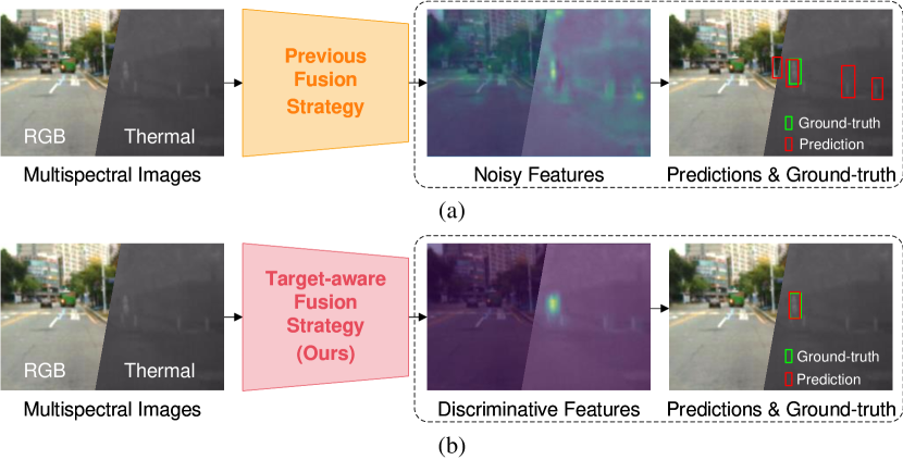
Recent works [3, 4, 5, 6, 7, 8, 9] demonstrate that the combination of multispectral features improves the accuracy of single-modality pedestrian detection. Moreover, the gain in accuracy largely depends on the fusion stage and the employed strategy. Previous studies [5, 10, 11, 12] reveal that the halfway fusion approach outperforms both early and late fusion approaches. The terms “early”, “halfway”, and “late” fusion refer to the fusion of multispectral information at the low, middle, and high stages of a two-branch network, respectively. Building upon this finding, recent works design complex halfway fusion strategies to address various challenges, such as misalignment [8, 13, 14], modality imbalance [9, 15] and ensemble learning [16] issues. However, a problem across these works is the generation of noisy fused features. The reason for this phenomenon is that the previous works primarily focus on combining complementary features from both modalities while neglecting to distinguish between target and non-target features. We have observed that these noisy features may lead to a significant number of false positives (FPs) and degrade performance, as shown in Fig. 1 (a). A more detailed analysis is presented in Section III-A.
To mitigate the adverse effect of noisy features, in this work we propose a target-aware fusion strategy. Within the framework of this strategy, we introduce a novel multispectral feature fusion module that leverages the inherent parallel-channel and cross-channel similarities found in paired multispectral features. Additionally, we propose a feature refinement module, which includes a feature classification unit and a feature contrast enhancement unit. Furthermore, we present a novel correlation-maximum loss function. These enhancements not only enable the model to combine complementary information but also to distinguish between target and non-target features, and improve representations in target regions while suppressing those in non-target regions. Benefiting from these modules, our target-aware fusion strategy empowers the model to effectively focus on target regions, thereby reducing FPs in the background regions, as illustrated in Fig. 1 (b).
The detector equipped with our target-aware fusion strategy for multispectral pedestrian detection is named TFDet. Our target-aware fusion strategy is flexible and can be applied to both one-stage and two-stage detectors. TFDet achieves state-of-the-art performance on two multispectral pedestrian detection benchmarks [1, 2], and more importantly, it demonstrates much greater superiority over previous methods under low-light conditions. Additionally, our fusion strategy is computationally efficient, which enables TFDet to generate predictions more quickly in traffic scenarios. In summary, our contributions are threefold:
-
•
We propose a new multispectral feature fusion method known as the target-aware fusion strategy. Different from previous fusion strategies, our method not only focuses on combining complementary features from both modalities but also explore feature refinement techniques to enhance the representations in target regions while suppressing those in non-target regions.
-
•
Our target-aware fusion strategy generates discriminative features and significantly reduces false positives in background regions. Meanwhile, our fusion strategy is flexible and can effectively benefit both one-stage and two-stage detectors.
-
•
Extensive experiments demonstrate that the detector equipped with our target-aware fusion strategy, named TFDet, achieves state-of-the-art performance on two challenging datasets. Additionally, TFDet achieves comparable inference time to previous state-of-the-art counterparts, demonstrating its efficiency.
II Related Work
In this section, we first briefly outline the works related to general object detection and pedestrian detection. Then, we introduce previous studies in the area of multispectral pedestrian detection.
II-A Object Detection and Pedestrian Detection
Object detectors can be categorized into two groups: one-stage detectors [17, 18] and two-stage detectors [19, 20], based on whether they require object proposals [21]. One-stage detectors directly predict object boxes, either by using anchors [22] or a grid of potential object centers [23]. YOLO [17] is a popular one-stage detector that takes the full-size image as input and simultaneously outputs the object boxes and class-specific confidence scores. Although one-stage detectors tend to be fast, their accuracy is somehow limited. In comparison, two-stage detectors frame object detection as a “coarse-to-fine” process. They predict object boxes based on region proposals [19]. In the first stage, the detector generates multiple object proposals, each indicating a potential object in an image region. In the second stage, the detector further refines the location and predicts the class scores for these proposals. Faster R-CNN [19] is a well-known two-stage detector. It consists of two components: RPN [19] and R-CNN [24]. The RPN component is trained end-to-end to generate high-quality region proposals, which are then used by R-CNN for object detection. Although two-stage detectors have high accuracy, they tend to be slower.
II-B Multispectral Pedestrian Detection
Multispectral pedestrian detection uses both RGB and thermal images to detect pedestrians [1, 2]. Its goal is to take advantage of the strengths of both RGB and thermal modalities and perform effectively and consistently under varying lighting conditions. However, simply concatenating RGB and thermal images as the input of detectors does not significantly improve the performance [5]. Therefore, recent works focus on effectively fusing multispectral features. These approaches can be categorized into two groups based on the requirement of box-level masks: one group requires box-level masks [4, 29, 3], while the other does not [5, 8, 9, 15, 7, 6, 16, 30].
In terms of detection without box-level masks, the work [5] focuses on finding better fusion architectures across different CNN stages. It shows that the half-fusion architecture, which fuses the mid-level features, is better than early-fusion and late-fusion architectures. Recent works build on this strategy and make further progress in improving detection accuracy from various perspectives. For instance, AR-CNN [8] addresses the weakly aligned problem. MBNet [9] tackles the modality imbalance issue, while SCDNet [15] focuses on refining multispectral features. BAANet [7] addresses the modality-specific noise problem. DCMNet [6] focuses on learning the local and non-local information between multispectral features, and ProbEn [16] explores the ensemble learning problem.
In comparison, another key paradigm is the detection with box-level masks. MSDS-RCNN [4] introduces a segmentation branch and trains the models using a multi-task loss function, including a detection and a segmentation loss. It employs the bounding-box annotations to generate binary masks and uses the masks to supervise the segmentation branch. Following a similar approach, GAFF [29] uses the box-level masks to guide the attention of intra-modality and inter-modality. Meanwhile, LG-FAPF [3] uses box segmentation in single modality as local guidance and fuses information from another modality.
Our TFDet differs from recent works in four main aspects: (1) TFDet builds upon the insight that noisy features result in FPs, and these FPs significantly impair performance. (2) TFDet not only focuses on fusing complementary features from both modalities but also on addressing the noisy feature issue. (3) For the purpose of feature fusion, TFDet is based on the inherent feature similarity in paired multispectral images. For the purpose of contrast enhancement, TFDet is based on the correlation between an initial fused feature and a target representation. (4) TFDet achieves a significant performance improvement over recent works and demonstrates its superiority under low-light scenes.
III Method
In this section, we first describe our motivation. Then, we present the mathematical principles behind our proposed target-aware fusion strategy in Section III-B. Subsequently, we provide an overview of TFDet in Section III-C and elaborate on its three key components: the feature fusion module (FFM) in Section III-D, the feature refinement module (FRM) in Section III-E, and the correlation-maximum loss function in Section III-F.
We are also interested in understanding the practical operational mechanisms of each module in our target-aware fusion strategy. However, a rigorous theoretical analysis of the representations learned by deep neural networks remains a challenging task. Therefore, we take an empirical approach to explore the role of each module. We describe the effect of FFM immediately after introducing the structure of FFM in Section III-D. Since the FRM and the correlation-maximum loss function are complementary for contrast enhancement during training, we describe their effects in Section III-F.
III-A Motivation
Our motivation arises from the observation that the detector can recall most of the ground-truth pedestrians but also generates many FPs in the background regions. As shown in Fig. 1 (a), the detector makes a correct prediction in the target region but generates three FPs in background regions. Nevertheless, previous works are more interested in the misalignment [14, 3] and modality imbalance [15, 30] issues, while overlooking the impact of FPs on detection performance.
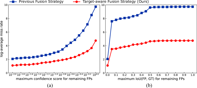
To analyze this impact, we conduct a pilot study. Specifically, we manually remove the FPs based on their (a) confidence scores and (b) intersection-over-union (IoU) rates with ground-truth boxes in descending order. The corresponding results are presented in Fig. 2. The log-average miss rate progressively decreases (lower values are better) as the FPs are removed. Furthermore, the log-average miss rate decreases rapidly when FPs with (a) high scores and (b) low IoU rates are removed. This reveals that FPs with high scores may be mainly distributed in the background regions, and these FPs are more detrimental. This phenomenon may be attributed to the similarity in shape between objects in the FPs’ regions and pedestrians, as shown in Fig. 1 (a). The shape similarity confuses the model, leading to the generation of noisy features and a number of FPs.
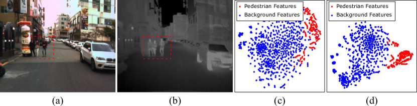
We propose a target-aware fusion strategy to address the noisy feature issue. The primary objective of our strategy is to enhance feature representations in target regions, while simultaneously suppressing those in non-target regions. To achieve this goal, we introduce a feature fusion module (FFM) to combine complementary features, a feature refinement module (FRM) to discriminate between target and non-target features, and a correlation-maximum loss function to enhance feature contrast. Our target-aware fusion strategy significantly reduces FPs, as shown in Fig. 2. Additionally, we showcase the feature visualizations of both the previous fusion strategy and our target-aware fusion strategy using t-distributed stochastic neighbor embedding (t-SNE) [31], as depicted in Fig. 3. Within the t-SNE map, our target-aware fusion strategy tightly clusters points of the same class and effectively separates those from different classes. This demonstrates that our fusion strategy can generate contrast-enhanced features.
III-B Foundation of Feature Contrast Enhancement
The mathematical foundation of the feature contrast enhancement in our fusion strategy is built upon the correlation between a ground-truth (GT) box-level mask and the initial fused feature. The initial fused feature is generated by a feature fusion module. Therefore, this feature contains full information from both modalities, but it is noisy. The box-level mask is generated by assigning 1s to the regions inside GT boxes and 0s to the other regions. This mask label not only helps pinpoint the location of targets but also saves time compared to pixel-level labeling. In this context, the intuition for contrast enhancement of the initial fused feature is to improve the aforementioned correlation in the channel dimension.
Denote the initial fused feature as and the GT box-level mask as . Since the GT mask is not available at test time, we learn to predict it using a segmentation branch. Denote the predicted mask as , we can compute the cosine similarity between the predicted mask and the initial fused feature across the channel dimension as
| (1) | ||||
where the initial fused feature is represented as a set . The operation computes the inner product between the predicted mask and the channel feature map . Since they are normalized, the inner product can indicate their similarities.
One straightforward method for enhancing feature contrast is to maximize each entry in the correlation . However, this method makes each feature map equal to the box-level mask, resulting in the loss of important semantic information across different channels. To address this issue, we introduce a projection matrix to encode the correlation and generate the processed correlation
| (2) |
where the symbol “T” represents a transpose operation.
In this context, an entry of the processed correlation can be written as
| (3) | ||||
Let , we can infer that
| (4) |
where denotes the element located at row and column within the matrix . This equation demonstrates that each entry represents the similarity between the predicted mask and the weighted average of initial fused feature across the channel dimension. Based on this analysis, we enforce each entry to approximate 1.0, thereby enhancing their correlation. Nevertheless, the mathematical process described above is linear, thus we use convolutional operations to implement the projection process in our target-aware fusion strategy. In addition, we introduce a correlation-maximum loss function, which includes a segmentation loss function and a negative correlation loss function, to supervise the predicted mask and the processed correlation.
III-C Architecture of TFDet
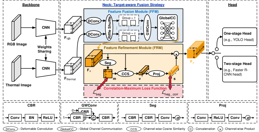
The overall architecture of our TFDet is illustrated in Fig. 4. We feed a pair of RGB and thermal images into a CNN backbone network to generate the corresponding multispectral features denoted as and . Subsequently, the multispectral features are fused in the neck part using our target-aware fusion strategy. In this fusion strategy, the FFM first adaptively combines the multispectral features, generating the initial fused feature denoted as . Based on this initial fused feature, the FRM then discriminates between the foreground and background features by employing an auxiliary segmentation branch. Following that, the FRM enhances feature contrast through the correlation-maximum loss function during training. Our target-aware fusion strategy finally yields the discriminative feature , which is subsequently fed into detection heads. These detection heads can be the one-stage head (such as YOLO head [22]) or the two-stage head (such as Faster R-CNN head [19], including the RPN and R-CNN). This process predicts boxes and corresponding scores.
Our target-aware fusion strategy is independent of the CNN structure. Different detectors often leverage various pyramid networks to fuse multi-scale features. For instance, Faster R-CNN employs FPN [32], while YOLOv5 utilizes PANet [33]. Due to this, we omit the schematic diagram of the pyramid networks in Fig. 4. Since we conduct the identical feature fusion process at different levels of the pyramid networks, we only provide a detailed description of the process at one level.
In this paper, we employ a weight-sharing CNN as the backbone network to extract multispectral features. This choice is motivated by its ability to save computation costs and the reduction in learnable parameters, which helps mitigate the potential effects of overfitting. Meanwhile, we also notice that certain works [34, 35, 15, 9, 3, 29] use different backbone networks for feature extraction. Nevertheless, such approaches often need to elaborately design complex training techniques to ensure the model’s effective generalization [35].
III-D Feature Fusion Module (FFM)
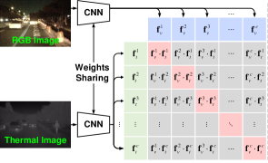
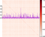
Observation. Our proposed FFM gains insights from the similarities in multispectral features. Specifically, given the multispectral features and , each of which contains channel maps with a resolution of , we exhaustively compute the inner product among all channel maps, obtaining a multispectral feature relation matrix of size . This process is depicted in Fig. 5 (a), where we denote the features and as and , respectively. From Fig. 5 (b), we can observe two enlightening phenomena: (1) elements along the diagonal have larger values, indicating a strong similarity between multispectral features at the same channel position, which we refer to as “parallel-channel similarity”, and (2) there are also large elements in the off-diagonal regions, suggesting that features across different channels may also exhibit strong similarity, which we term as “cross-channel similarity”.
To comprehensively verify whether the similarities in multispectral features are universal, we define two metrics: the Average Mean Ratio (ANR) and the Average Median Ratio (AIR). These metrics are designed to summarize the differences between diagonal and off-diagonal elements. The ANR computes the average ratio between the element at the diagonal position and the mean of those at the off-diagonal positions across the entire dataset. Meanwhile, the AIR employs a similar approach but utilizes the median value of the off-diagonal elements as the denominator. The mathematical process can be formulated as
| (5) | ||||
and
| (6) |
where represents the number of paired RGB-T images in a dataset, and the entry denotes the index of the image pair. For each image pair, computes the inner product of multispectral features at channel position . The operators Mean() and Median() return the mean and median values of the given sets, respectively. We select the mean and median values as denominators for two reasons: (1) the mean value reflects the overall expectation of elements at off-diagonal positions, and (2) the median value avoids the influence of outliers.
Based on the aforementioned definition, we calculate ANR and AIR on two representative datasets: KAIST [1] and LLVIP [2]. Detailed statistics for these two datasets are provided in Section IV-A. The results presented in Table I reveal two phenomena: (1) both the ANR and AIR exceed 1, indicating strong parallel-channel similarity, and (2) ANR consistently tends to be smaller than AIR, implying a strong cross-channel similarity.
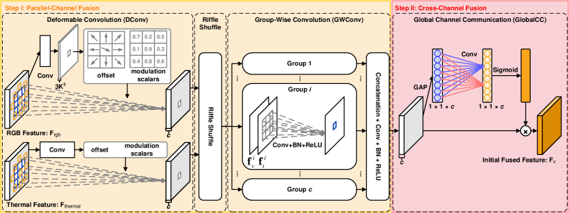
Feature Fusion Module Structure. Based on the universal parallel- and cross-channel similarities in multispectral features, we propose a two-step method for fusing these features, as illustrated in Fig. 6. In the first step, we employ the property of parallel-channel similarity to fuse two corresponding channel features. Considering the diverse scales of pedestrians at varying distances from cameras, we adopt deformable convolution (DConv) [36] to adaptively learn receptive field for each output response. However, since the DConv is originally designed for single-modality inputs, we propose a modification involving riffle shuffle and group-wise convolution (GWConv) to tailor it for multispectral features. In the second step, we exploit the property of cross-channel similarity to recalibrate channel-wise features. For this purpose, we introduce a global channel communication (GlobalCC) block, which explicitly constructs interdependencies between channels, producing a set of modulation weights. These weights are then applied to the feature obtained in Step I, yielding the initial fused feature .
| Method | MR () |
|---|---|
| Fixed-RP | 9.90 |
| Adaptive-RP | 8.96 |
| Adaptive-RP + ConvCC | 8.94 |
| FFM (Adaptive-RP + GlobalCC) | 8.57 |
Effect Validation: Adaptive Receptive Field (Adaptive-RP). We evaluate our modified DConv’s ability in adaptively learning receptive fields. In Fig. 7, we visualize how sampling locations change with object variations, indicating adaptive receptive field behavior. We also compare Adaptive-RP with a fixed receptive field variant called Fixed-RP in Table II, which uses two convolutional operations to replace the DConv. This comparison demonstrates the superiority of our Adaptive-RP.
Effect Validation: Effect of Global Chanel Communication. To assess the impact of GlobalCC, we replace it with a convolution called ConvCC. The results in Table II show that our FFM, which incorporates Adaptive-RP and GlobalCC, achieves superior performance due to GlobalCC’s capacity to capture a global receptive field via global average pooling (GAP), unlike ConvCC with its fixed-sized kernel.
III-E Feature Refinement Module (FRM)
We propose FRM to enhance the contrast between pedestrian-related features and background features. FRM takes the initially fused feature as input, and outputs the contrast-enhanced feature . Specifically, we first generate the box-level mask label based on the bounding-box annotations by filling pedestrian areas with 1s and the remaining areas with 0s. Next, we use the feature to predict the box-level mask through a segmentation (Seg) branch. This process is defined as
| (7) |
where the function denotes the segmentation branch, and the function represents a sigmoid activation.
We then compute the correlation between the predicted box-level mask and the feature along the channel direction, which is defined in (1). This correlation is processed by a projection (Proj) layer to generate the processed correlation
| (8) |
where the function represents the projection layer, which consists of two convolutional operations. We then use it to scale the feature and generate the refined feature
| (9) |
where the operation performs channel-wise product. Throughout the refinement process, we supervise the predicted box-level mask and maximize the processed correlation using our correlation-maximum loss function.
III-F Correlation-Maximum Loss Function
Based on the analysis in Section III-B, our feature contrast enhancement method needs to ensure that: (1) the predicted box-level mask is as accurate as possible, and (2) the processed correlation between the predicted box-level mask and the initially fused feature is as high as possible. Since the ground-truth box-level mask is binary and exhibits distinct contrast between the foreground and background, this method enables the detector to learn contrast-enhanced features.
To this end, we propose a novel loss function named the correlation-maximum loss function to regularize the model. It is defined as
| (10) |
where denotes the GT box-level mask and in this work. This function comprises two components: the segmentation loss function and the negative correlation loss function .
The segmentation loss function aims to maximize the accuracy of the predicted box-level mask. It is defined as
| (11) |
The binary cross-entropy loss function [37] is defined as
| (12) |
where
| (13) |
The dice loss function [38] is defined as
| (14) | ||||
where and denote the elements of and at the location , respectively. is set to 1.0 following the setting in [38]. We use nearest neighbor method to down-sample the GT box-level mask to match the shape of the predicted mask. computes their intersection, and computes the magnitude of a mask.
The negative correlation loss function aims to make each entry in the processed correlation approach 1.0. It is defined as
| (15) |
Since the logarithm function often generates larger gradients when is close to zero compared to the -norm-based (e.g., mean absolute error) and -norm-based (e.g., mean squared error) loss functions, we construct the negative correlation loss function in the log domain. We combine the correlation-maximum losses from multiple CNN stages with the final detection losses, including classification and regression losses, to train the detectors.
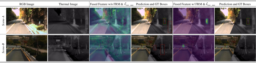
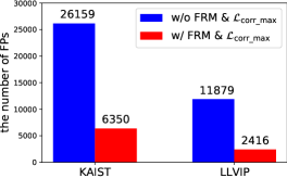
Effect Validation: FRM and Correlation-Maximum Loss Function. The purpose of our proposed FRM and the correlation-maximum loss function is to reduce FPs by enhancing the feature contrast between foreground and background regions. To understand their effects, we compare feature visualization results between the method with and without FRM and the correlation-maximum loss function, respectively, denoted as “w/ FRM ” and “w/o FRM ” for simplicity. Fig. 8 shows that FRM and the correlation-maximum loss function effectively enhance the feature contrast while the counterpart generates noisy feature maps and FPs. Furthermore, we count the FPs across entire datasets. The results in Fig. 9 show that our method significantly reduces the FPs on different datasets.
IV Experiments
| Method | Publication Year | All-Day() | Day() | Night() | Near() | Medium() | Far() |
|---|---|---|---|---|---|---|---|
| IAF-RCNN [40] | Pattern Recognition 2019 | 15.73 | 14.55 | 18.26 | 0.96 | 25.54 | 77.84 |
| IATDNN+IAMSS [41] | Information Fusion 2019 | 14.95 | 14.67 | 15.72 | 0.04 | 28.55 | 83.42 |
| IAHDANet [30] | TITS 2023 | 14.65 | 18.88 | 5.92 | - | - | - |
| CIAN [42] | Information Fusion 2019 | 14.12 | 14.77 | 11.13 | 3.71 | 19.04 | 55.82 |
| MSR [43] | AAAI 2022 | 11.39 | 15.28 | 6.48 | - | - | - |
| TINet [34] | TIM 2023 | 10.25 | 7.48 | 9.15 | - | - | - |
| AR-CNN [8] | ICCV 2019 | 9.34 | 9.94 | 8.38 | 0.00 | 16.08 | 69.00 |
| CMPD [44] | TMM 2022 | 8.16 | 8.77 | 7.31 | 0.00 | 12.99 | 51.22 |
| MBNet [9] | ECCV 2020 | 8.13 | 8.28 | 7.86 | 0.00 | 16.07 | 55.99 |
| SCDNet [15] | TITS 2022 | 8.07 | 8.16 | 7.51 | - | - | - |
| BAANet [7] | ICRA 2022 | 7.92 | 8.37 | 6.98 | 0.00 | 13.72 | 51.25 |
| UCG [13] | TCSVT 2022 | 7.89 | 8.00 | 6.95 | 1.07 | 11.36 | 37.16 |
| MFPT [14] | TITS 2023 | 7.72 | 8.26 | 4.53 | - | - | - |
| MLPD [45] | IEEE RA-L 2021 | 7.58 | 7.95 | 6.95 | 0.00 | 12.10 | 52.79 |
| MSDS-RCNN [4] | BMVC 2018 | 7.49 | 8.09 | 5.92 | 1.07 | 12.33 | 58.55 |
| SMPD [46] | TCSVT 2023 | 7.44 | 8.12 | 6.23 | 0.00 | 11.04 | 54.92 |
| GAFF [29] | WACV 2021 | 6.48 | 8.35 | 3.46 | 0.00 | 13.23 | 46.87 |
| VTFYOLO [47] | TII 2023 | 6.48 | 6.65 | 5.82 | - | - | - |
| DCMNet [6] | ACM MM 2022 | 5.84 | 6.48 | 4.60 | 0.02 | 16.07 | 69.70 |
| ProbEn3 w/GAFF [16] | ECCV 2022 | 5.14 | 6.04 | 3.59 | 0.00 | 9.59 | 41.92 |
| LG-FAPF [3] | Information Fusion 2022 | 5.12 | 5.83 | 3.69 | 0.58 | 8.44 | 40.47 |
| TFDet (Ours) | - | 4.47 | 5.22 | 3.36 | 0.00 | 9.29 | 55.50 |
In this section, we evaluate the performance of TFDet on two representative multispectral pedestrian detection datasets through a series of experiments. These experiments include: (1) extensive comparisons of our method with various state-of-the-art counterparts under identical experimental conditions, (2) the presentation of visualization examples, and (3) an ablation study. The objective of these experiments is to demonstrate the effectiveness of TFDet and to gain insights into its mechanism.
IV-A Datasets
The KAIST [1] dataset is a widely used multispectral pedestrian detection dataset. Recent works [4, 5] have updated this dataset because original version contains noisy annotations. The updated dataset includes 7,601 pairs of aligned RGB and thermal images in the training set and 2,252 in the validation set, each with a spatial resolution of 512 640.
The LLVIP [2] dataset is a more challenging multispectral pedestrian detection dataset. It is taken under low-light conditions, making it difficult to detect pedestrians in the RGB modality. This dataset includes 12,025 pairs of aligned RGB-T images in the training set and 3,463 in the validation set, with each image having a resolution of 1,024 1,280.
IV-B Implementation Details
In our experiments, we employ Faster R-CNN [19] and YOLOv5 [22] as two-stage and one-stage detectors, respectively. We implement Faster R-CNN using the MMDetection [50] toolbox, and utilize the official repository of YOLOv5 [22]. Unless otherwise specified, all experiments are run on two GTX 3090 GPUs. For Faster R-CNN, we train for 12 epochs with a total batch size of 6 and an initial learning rate of 0.01, using SGD optimizer. The learning rate is decayed by a factor of 0.1 at epoch 8 and epoch 11. Data augmentation is performed with random horizontal flipping. For YOLOv5, we train for 100 epochs and use the hyperparameters specified in the official configuration file. In addition, to ensure a fair comparison with existing approaches, we adopt the same detectors, backbone networks, and evaluation metrics used in prior works.
For the KAIST dataset, we adopt Faster R-CNN with VGG-16 [39] as the baseline detector, following the practices in [40, 5, 41, 42, 4, 8, 6, 3]. To evaluate the performance of detectors, we calculate the log-average miss rate (MR) [51] using a commonly-used toolbox provided in [4]. A lower MR indicates better detection performance.
For the LLVIP dataset, we use Faster R-CNN with ResNet-50 [48] and YOLOv5-Large [22] as the baseline detectors, following the practices in [49, 6, 2]. Model performance is evaluated using the average precision metric, with and denoting the average precision at and , respectively. The AP is calculated by averaging over 10 IoU thresholds ranging from 0.50 to 0.95 with 0.05 interval. A higher AP indicates better detection performance.
IV-C Comparison on the KAIST Dataset
We compare TFDet with 21 state-of-the-art approaches on the KAIST dataset [1], and present the results in Table III. The results demonstrate that TFDet achieves state-of-the-art performance, as all competitors generally pursue a lower MR in the All-Day subset. To the best of our knowledge, TFDet is the first method to achieve an MR level lower than 5%.
Notably, TFDet exhibits significant superiority in the Night subset, where RGB images are basically of poor visual quality. Such conditions make pedestrian detection more challenging.
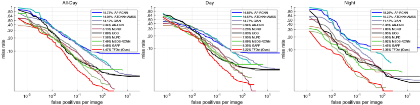
To comprehensively analyze these superiorities, we plot the miss rate versus false positives per image (FPPI) curves in Fig. 10. The results show that TFDet misses fewer pedestrians even when the confidence threshold is high (i.e., FPPI is low).
IV-D Comparison on the LLVIP Dataset
We compare our TFDet with four state-of-the-art approaches [49, 6, 16, 2] on the LLVIP dataset [2]. To ensure a fair comparison, we use the same resolutions, detectors, backbone networks and evaluation metrics as the counterparts.
In Table IV, we compare TFDet with approaches that use a single modality [2], as well as a baseline method that fuses RGB and thermal modalities in the feature space. The results confirm that fusing complementary information benefits the detection. Additionally, TFDet achieves the highest performance in term of APIoU=.75 and AP, indicating that it is more precise in locating pedestrians.
IV-E Inference Time
We test the inference time of TFDet on the KAIST dataset at a resolution of 512 640. Since we use Faster R-CNN [19] with VGG-16 [39] as the baseline detector for this dataset, we compare our results with approaches that have the same settings [4, 41, 40, 8, 6]. These approaches are tested on a single TitanX GPU according to [6]. To ensure a fair comparison, we use an RTX 3060 GPU in this experiment. According to the public documentation111https://www.mydrivers.com/zhuanti/tianti/gpu/index.html, it is confirmed that they have equivalent computing power.
IV-F Qualitative Comparisons
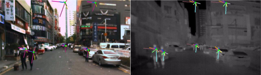
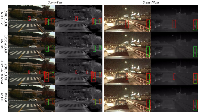
To comprehensively understand the effectiveness of TFDet, we conduct qualitative comparisons with state-of-the-art approaches. AR-CNN [8], MBNet [9], and ProbEn [16] are selected as counterparts on the KAIST dataset, whose results are publicly available. Fig. 11 presents these comparisons on two scenes (day and night). The results show that the counterparts generate unwanted FPs, such as red boxes in the background or replicated boxes on pedestrians, as well as false negatives (i.e., missed pedestrians). In contrast, TFDet successfully detects all pedestrians in both scenes.
IV-G Ablation Study
| Method | FFM | FRM | MR () | ||
|---|---|---|---|---|---|
| Ablation | ✓ | 8.57 | |||
| ✓ | ✓ | 6.82 | |||
| ✓ | ✓ | ✓ | 5.41 | ||
| TFDet (Ours) | ✓ | ✓ | ✓ | ✓ | 4.47 |
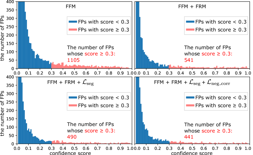
We conduct an ablation study to evaluate the effect of each module in our target-aware fusion strategy. The results, shown in Table VII, indicate that our TFDet, which uses FFM, FRM, and the correlation-maximum loss function (including and ), performs the best. Furthermore, we present the distribution of FPs’ confidence scores in Fig. 12. To facilitate comparison, we mark the bars with scores greater than 0.3 in red and display their quantities in the figure. The correspondence between the decrease in the number of FPs in Fig. 12 and the performance improvement in Table VII confirms the importance of reducing FPs.
V Conclusions
In this work, we address the challenge of feature fusion in the multispectral pedestrian detection task. We find that false positives (FPs) caused by noisy features significantly deteriorate detection performance, which has been overlooked by previous works. To address the issue of noisy features, we propose a target-aware fusion strategy for the detection task, named TFDet. Within this strategy, we introduce a feature fusion module (FFM) to collect complementary features, a feature refinement module (FRM) to distinguish between pedestrian and background features, and a correlation-maximum loss function to enhance feature contrast. Visualization results demonstrate that our fusion strategy generates discriminative features and significantly reduces FPs. As a result, TFDet achieves state-of-the-art performance on two benchmarks. Additionally, our strategy is flexible and computationally efficient, allowing it to be applied to both one-stage and two-stage detectors while maintaining low inference time.
References
- [1] S. Hwang, J. Park, N. Kim, Y. Choi, and I. So Kweon, “Multispectral Pedestrian Detection: Benchmark Dataset and Baseline,” in Proceedings of the IEEE Conference on Computer Vision and Pattern Recognition (CVPR), 2015.
- [2] X. Jia, C. Zhu, M. Li, W. Tang, and W. Zhou, “LLVIP: A Visible-Infrared Paired Dataset for Low-Light Vision,” in Proceedings of the IEEE International Conference on Computer Vision (ICCV), 2021.
- [3] Y. Cao, X. Luo, J. Yang, Y. Cao, and M. Y. Yang, “Locality Guided Cross-Modal Feature Aggregation and Pixel-Level Fusion for Multispectral Pedestrian Detection,” Information Fusion, 2022.
- [4] C. Li, D. Song, R. Tong, and M. Tang, “Multispectral Pedestrian Detection via Simultaneous Detection and Segmentation,” in British Machine Vision Conference (BMVC), 2018.
- [5] J. Liu, S. Zhang, S. Wang, and D. Metaxas, “Multispectral Deep Neural Networks for Pedestrian Detection,” in British Machine Vision Conference (BMVC), 2016.
- [6] J. Xie, R. M. Anwer, H. Cholakkal, J. Nie, J. Cao, J. Laaksonen, and F. S. Khan, “Learning a Dynamic Cross-Modal Network for Multispectral Pedestrian Detection,” in Proceedings of the ACM International Conference on Multimedia (ACM MM), 2022.
- [7] X. Yang, Y. Qian, H. Zhu, C. Wang, and M. Yang, “BAANet: Learning Bi-Directional Adaptive Attention Gates for Multispectral Pedestrian Detection,” in International Conference on Robotics and Automation (ICRA), 2022.
- [8] L. Zhang, X. Zhu, X. Chen, X. Yang, Z. Lei, and Z. Liu, “Weakly Aligned Cross-Modal Learning for Multispectral Pedestrian Detection,” in Proceedings of the IEEE International Conference on Computer Vision (ICCV), 2019.
- [9] K. Zhou, L. Chen, and X. Cao, “Improving Multispectral Pedestrian Detection by Addressing Modality Imbalance Problems,” in Proceedings of the European Conference on Computer Vision (ECCV), 2020.
- [10] L. Zhang, Z. Liu, X. Zhu, Z. Song, X. Yang, Z. Lei, and H. Qiao, “Weakly Aligned Feature Fusion for Multimodal Object Detection,” IEEE Transactions on Neural Networks and Learning Systems, 2021.
- [11] H. Fu, S. Wang, P. Duan, C. Xiao, R. Dian, S. Li, and Z. Li, “LRAF-Net: Long-Range Attention Fusion Network for Visible-Infrared Object Detection,” IEEE Transactions on Neural Networks and Learning Systems, 2023.
- [12] J. Zhang, H. Liu, K. Yang, X. Hu, R. Liu, and R. Stiefelhagen, “CMX: Cross-Modal Fusion for RGB-X Semantic Segmentation with Transformers,” IEEE Transactions on Intelligent Transportation Systems, 2023.
- [13] J. U. Kim, S. Park, and Y. M. Ro, “Uncertainty-Guided Cross-Modal Learning for Robust Multispectral Pedestrian Detection,” IEEE Transactions on Circuits and Systems for Video Technology, 2022.
- [14] Y. Zhu, X. Sun, M. Wang, and H. Huang, “Multi-Modal Feature Pyramid Transformer for RGB-Infrared Object Detection,” IEEE Transactions on Intelligent Transportation Systems, 2023.
- [15] K. Dasgupta, A. Das, S. Das, U. Bhattacharya, and S. Yogamani, “Spatio-Contextual Deep Network-Based Multimodal Pedestrian Detection for Autonomous Driving,” IEEE Transactions on Intelligent Transportation Systems, 2022.
- [16] Y.-T. Chen, J. Shi, Z. Ye, C. Mertz, D. Ramanan, and S. Kong, “Multimodal Object Detection via Probabilistic Ensembling,” in Proceedings of the European Conference on Computer Vision (ECCV), 2022.
- [17] J. Redmon, S. Divvala, R. Girshick, and A. Farhadi, “You Only Look Once: Unified, Real-Time Object Detection,” in Proceedings of the IEEE Conference on Computer Vision and Pattern Recognition (CVPR), 2016.
- [18] N. Carion, F. Massa, G. Synnaeve, N. Usunier, A. Kirillov, and S. Zagoruyko, “End-to-End Object Detection with Transformers,” in Proceedings of the European Conference on Computer Vision (ECCV), 2020.
- [19] S. Ren, K. He, R. Girshick, and J. Sun, “Faster R-CNN: Towards Real-Time Object Detection with Region Proposal Networks,” in Advances in Neural Information Processing Systems, 2015.
- [20] P. Sun, R. Zhang, Y. Jiang, T. Kong, C. Xu, W. Zhan, M. Tomizuka, L. Li, Z. Yuan, C. Wang, and P. Luo, “Sparse R-CNN: End-to-End Object Detection with Learnable Proposals,” in Proceedings of the IEEE Conference on Computer Vision and Pattern Recognition (CVPR), 2021.
- [21] Z. Zou, K. Chen, Z. Shi, Y. Guo, and J. Ye, “Object Detection in 20 Years: A Survey,” Proceedings of the IEEE, 2023.
- [22] G. Jocher, “YOLOv5 by Ultralytics,” 2020. [Online]. Available: https://github.com/ultralytics/yolov5
- [23] Z. Tian, C. Shen, H. Chen, and T. He, “FCOS: Fully Convolutional One-Stage Object Detection,” in Proceedings of the IEEE International Conference on Computer Vision (ICCV), 2019.
- [24] R. Girshick, “Fast R-CNN,” in Proceedings of the IEEE International Conference on Computer Vision (ICCV), 2015.
- [25] W. Liu, I. Hasan, and S. Liao, “Center and Scale Prediction: Anchor-Free Approach for Pedestrian and Face Detection,” Pattern Recognition, 2023.
- [26] W. Liu, S. Liao, and W. Hu, “Efficient Single-Stage Pedestrian Detector by Asymptotic Localization Fitting and Multi-Scale Context Encoding,” IEEE Transactions on Image Processing, 2020.
- [27] I. Hasan, S. Liao, J. Li, S. U. Akram, and L. Shao, “Generalizable Pedestrian Detection: The Elephant in the Room,” in Proceedings of the IEEE Conference on Computer Vision and Pattern Recognition (CVPR), 2021.
- [28] X. Huang, Z. Ge, Z. Jie, and O. Yoshie, “NMS by Representative Region: Towards Crowded Pedestrian Detection by Proposal Pairing,” in Proceedings of the IEEE Conference on Computer Vision and Pattern Recognition (CVPR), 2020.
- [29] H. Zhang, E. Fromont, S. Lefèvre, and B. Avignon, “Guided Attentive Feature Fusion for Multispectral Pedestrian Detection,” in Proceedings of the IEEE Winter Conference on Applications of Computer Vision (WACV), 2021.
- [30] Q. Xie, T.-Y. Cheng, Z. Dai, V. Tran, N. Trigoni, and A. Markham, “Illumination-Aware Hallucination-Based Domain Adaptation for Thermal Pedestrian Detection,” IEEE Transactions on Intelligent Transportation Systems, 2023.
- [31] L. Van der Maaten and G. Hinton, “Visualizing Data Using t-SNE,” Journal of Machine Learning Research, 2008.
- [32] T.-Y. Lin, P. Dollar, R. Girshick, K. He, B. Hariharan, and S. Belongie, “Feature Pyramid Networks for Object Detection,” in Proceedings of the IEEE Conference on Computer Vision and Pattern Recognition (CVPR), 2017.
- [33] S. Liu, L. Qi, H. Qin, J. Shi, and J. Jia, “Path Aggregation Network for Instance Segmentation,” in Proceedings of the IEEE Conference on Computer Vision and Pattern Recognition (CVPR), 2018.
- [34] Y. Zhang, H. Yu, Y. He, X. Wang, and W. Yang, “Illumination-Guided RGBT Object Detection with Inter- and Intra-Modality Fusion,” IEEE Transactions on Instrumentation and Measurement, 2023.
- [35] R. Zhang, L. Li, Q. Zhang, J. Zhang, L. Xu, B. Zhang, and B. Wang, “Differential Feature Awareness Network within Antagonistic Learning for Infrared-Visible Object Detection,” IEEE Transactions on Circuits and Systems for Video Technology, 2023.
- [36] X. Zhu, H. Hu, S. Lin, and J. Dai, “Deformable ConvNets v2: More Deformable, Better Results,” in Proceedings of the IEEE Conference on Computer Vision and Pattern Recognition (CVPR), 2019.
- [37] X. Zhang, Z. Sheng, and H.-L. Shen, “FocusNet: Classifying Better by Focusing on Confusing Classes,” Pattern Recognition, 2022.
- [38] F. Milletari, N. Navab, and S.-A. Ahmadi, “V-Net: Fully Convolutional Neural Networks for Volumetric Medical Image Segmentation,” in International Conference on 3D Vision (3DV), 2016.
- [39] K. Simonyan and A. Zisserman, “Very Deep Convolutional Networks for Large-Scale Image Recognition,” in International Conference on Learning Representations (ICLR), 2015.
- [40] C. Li, D. Song, R. Tong, and M. Tang, “Illumination-Aware Faster R-CNN for Robust Multispectral Pedestrian Detection,” Pattern Recognition, 2019.
- [41] D. Guan, Y. Cao, J. Yang, Y. Cao, and M. Y. Yang, “Fusion of Multispectral Data Through Illumination-Aware Deep Neural Networks for Pedestrian Detection,” Information Fusion, 2019.
- [42] L. Zhang, Z. Liu, S. Zhang, X. Yang, H. Qiao, K. Huang, and A. Hussain, “Cross-Modality Interactive Attention Network for Multispectral Pedestrian Detection,” Information Fusion, 2019.
- [43] J. U. Kim, S. Park, and Y. M. Ro, “Towards Versatile Pedestrian Detector with Multisensory-Matching and Multispectral Recalling Memory,” Proceedings of the AAAI Conference on Artificial Intelligence (AAAI), 2022.
- [44] Q. Li, C. Zhang, Q. Hu, H. Fu, and P. Zhu, “Confidence-Aware Fusion using Dempster-Shafer Theory for Multispectral Pedestrian Detection,” IEEE Transactions on Multimedia, 2022.
- [45] J. Kim, H. Kim, T. Kim, N. Kim, and Y. Choi, “MLPD: Multi-Label Pedestrian Detector in Multispectral Domain,” IEEE Robotics and Automation Letters, 2021.
- [46] Q. Li, C. Zhang, Q. Hu, P. Zhu, H. Fu, and L. Chen, “Stabilizing Multispectral Pedestrian Detection with Evidential Hybrid Fusion,” IEEE Transactions on Circuits and Systems for Video Technology, 2023.
- [47] X. Zou, T. Peng, and Y. Zhou, “UAV-Based Human Detection with Visible-Thermal Fused YOLOv5 Network,” IEEE Transactions on Industrial Informatics, 2023.
- [48] K. He, X. Zhang, S. Ren, and J. Sun, “Deep Residual Learning for Image Recognition,” in Proceedings of the IEEE Conference on Computer Vision and Pattern Recognition (CVPR), 2016.
- [49] Y. Sun, B. Cao, P. Zhu, and Q. Hu, “DetFusion: A Detection-Driven Infrared and Visible Image Fusion Network,” in Proceedings of the ACM International Conference on Multimedia (ACM MM), 2022.
- [50] MMDetection Contributors, “OpenMMLab Detection Toolbox and Benchmark,” 2018. [Online]. Available: https://github.com/open-mmlab/mmdetection
- [51] P. Dollar, C. Wojek, B. Schiele, and P. Perona, “Pedestrian Detection: An Evaluation of the State of the Art,” IEEE Transactions on Pattern Analysis and Machine Intelligence, 2012.