Holography and the Page curve of an evaporating black hole

Abstract

We consider a radiating black hole with a holographic dual such that its entanglement entropy does not exceed the Bekenstein-Hawking entropy, to obtain a Page curve. We make use of some mathematical identities that should be held for the entanglement entropy to be well-defined. This work is not going to give a resolution to the information paradox. Rather it shows that the general shape of the Page curve is a consequence of holography, independent of the details of gravitation theory.

1 Introduction

In 1975, Hawking studied quantum field theory in curved spacetime and showed that black holes radiate and hence lose their masses Hawking1975 ; Page1976 . This is in accord with the former obtained temperature of black holes, $T=\kappa/2\pi$, where $\kappa$ is black hole’s surface gravity Bekenstein1972 ; Bardeen1973 ; Page2005 . Then he proposed a paradox which was concerning the conservation of quantum information and predictability Hawking1976 . In fact, he showed that the black hole formation and evaporation process cause pure states to evolve into mixed states. Hence it destroys quantum information and is not a unitary process. A quantity called “von Neumann entropy” or “fine-grained entropy” or “entanglement entropy” is used to express the information loss amount quantitatively, which is defined as $S_{R}=-\Tr\rho_{R}\ln\rho_{R}$, where $\rho_{R}$ is the density matrix of the radiation. One would expect this quantity to rise at initial stages of the evaporation due to the entanglement between the radiation emitted and the remained black hole. However, in the case of starting from a black hole in a pure state, it should fall down after a time and eventually hit zero for the process to be unitary. Such a curve is suggested by Page by considering the thermodynamic entropies of radiation and black hole and switching between them as is shown in fig. 1 Page1983 ; Page1993 ; Page2013 . According to the Page curve, although the entanglement entropy of radiation follows Hawking’s calculation at first, after a time called Page-time—when the thermodynamic entropies of radiation and black hole become equal—it turns to follow the thermodynamic entropy of the black hole, which is given by the Bekenstein-Hawking formula, $S=\text{Area}/4G$ (there are several ways to obtain this formula microscopically Strominger1996 ; tHooft1985 ; Srednicki1993 ; Bombelli1986 ; Bena2022 ; Balasubramanian2022 ).

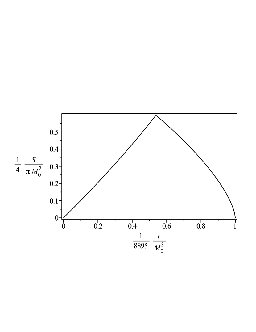
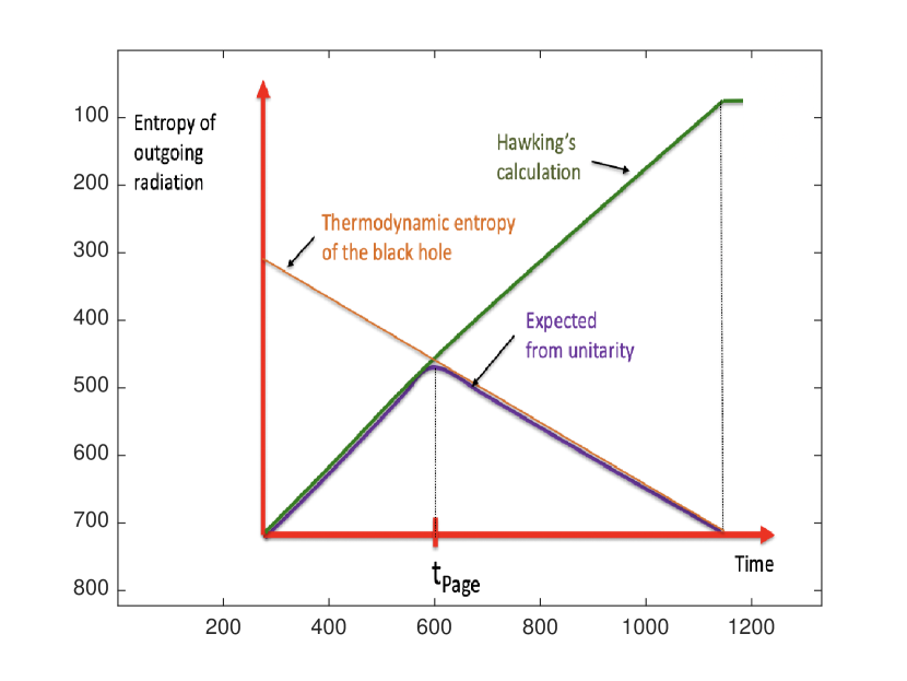
Figure 1: Left: The curve that Page suggested for entanglement entropy of the radiation emitted from a black hole initially in a pure state, from Page2013 . This curve is produced by considering the thermodynamic entropies of the radiation and the black hole as functions of time, and choosing the one that is less. Right: A schematic visualization of Page’s procedure in obtaining the Page curve, from Almheiri2021 . As is shown, the true curve for entanglement entropy of the radiation is expected to follow the thermodynamic entropy of the radiation at first. However, when reaching the Page time, it should switch to follow the thermodynamic entropy of the black hole. Obviously this curve is consistent with unitarity.

Much attempts made to resolve the paradox and obtain Page curve which finally led to the so-called “island formula” for entanglement entropy of the radiation Almheiri2019 ; Almheiri2020 ; Almheiri2020a ; Penington2020 . One can see, in the language of path-integral, that Hawking’s calculations neglect some paths which although are tiny at initial stages of the evaporation process, become dominated at final ones. The following relation is obtained for entanglement entropy in gravitational systems

$$S=\text{min}_{X}\left\{\text{ext}_{X}\left[\frac{\text{Area}(X)}{4G}+S_{\text{semi-cl}}\left(\Sigma_{X}\right)\right]\right\},$$ (1)

where $X$ is a codimension-2 surface and $\Sigma_{X}$ is the region bounded by $X$ and the surface from where we can almost assume that spacetime is flat, called cutoff surface. Moreover, $S_{\text{semi-cl}}$ is the von Neumann entropy of quantum fields on $\Sigma_{X}$, appearing in semiclassical description Ryu2006 ; Ryu2006a ; Hubeny2007 ; Engelhardt2015 ; Faulkner2013 (a good review is presented in Almheiri2021 ). Any surface that extremizes the expression in the square brackets is called “quantum extremal surface” (QES). It can be shown that there are two such surfaces present in the evaporation process, one with vanishing area and the other tending to the event horizon of the black hole from below. At the initial stages of the evaporation process, the first one can be found to be the minimizing QES which represents the no-island solution. However, after a time (Page time) the other one becomes dominated, representing the so-called island solution—due to the presence of a non-vanishing surface inside the black hole.

The precise state of the radiation is determined by the details of the evaporation process that made it. So, although gravitational interactions can be ignored in the radiation region $\Sigma_{\text{rad}}$ (from the cutoff surface all the way to infinity), the precise state of the radiation can only be determined via gravity. Thus one should again make use of Eq. (1) for truly computing the entanglement entropy of the emitted radiation. It should be noticed that the term $\Sigma_{X}$ for the radiation consists of: i) $\Sigma_{\text{rad}}$ and ii) $\Sigma_{\text{island}}$—the region inside the island. According to the literature, “island” is a region that is disconnected from the radiation region but contributing in its entanglement entropy in the form of Eq. (1). Having the initial black hole in a pure state causes the QES’s of the radiation to be identical with those of the black hole. In this work, we assume the initial black hole to be in a pure state, so that we could take the entanglement entropies of the radiation and the black hole to be identical.

The thermodynamic entropy of a black hole is given by the Bekenstein-Hawking formula, $S=A/4G$. It scales with the radius squared and not cubed, which means that the description of that volume of space can be thought of as encoded on its lower-dimensional boundary. This property is well understood in AdS/CFT correspondence—the most successful realization of the holographic principle—as there is a bijective isometry between the two theories in two spaces with different dimensions: a theory of gravity in a $(d+1)$-dimensional AdS bulk and a quantum field theory with conformal symmetry living on its $d$-dimensional boundary Hooft1993 ; Maldacena1997 ; Witten1998 . Moreover, AdS/CFT correspondence plays a central role in derivation of Eq. (1). In fact, this relation is based on the so-called RT/HRT/EW bulk reconstruction, which itself is studied and formulated in the light of AdS/CFT correspondence Ryu2006 ; Ryu2006a ; Hubeny2007 ; Engelhardt2015 ; Rangamani2016 . Therefore a question rises: To what extent does the Page curve depend on the holographic assumptions made? In other words, is it possible to obtain the Page curve directly from the holographic principle? In this work we want to find a suitable answer to such a question. Specifically, we consider holography in form of the following assumptions, to obtain a curve for entanglement entropy of an evaporating $(3+1)$-dimensional black hole: 1) There exists a system described by usual field theories and holographically dual to the black hole; 2) The black hole’s entanglement entropy will not exceed the Bekenstein-Hawking entropy Flanagan1999 ; Bousso2003 ; Bekenstein2005 ; Casini2008 ; Chen2008 ; Horwitz2022 . Making use of the assumptions, we obtain a curve that is similar to the Page curve in its general shape, i.e., i) It rises for times less than a specific time ($t_{\text{Page}}$); ii) It falls for times after that time and iii) It vanishes when the evaporation process is completed. However, some details of the curve, such as its limiting behavior in initial times, will depend on the details of the gravitation theory.

It is obvious, from the $2^{\text{nd}}$ assumption, that this work is not going to give a resolution to the information paradox. Rather it shows that the Page curve can be regarded as a consequence of the holographic assumptions made and model-independent to a very good extent. As the Page curve conserves unitarity for the evaporation process, one might think about the questions as finding the relationship between holography and unitarity, if there exists any. Some discussions are presented in Giddings2020 on this subject. Moreover, some conditions for the entanglement entropy to be compatible with causality are presented in Headrick2014 .

This paper is organized as follows: In Sec. 2, we discuss the function of a mathematical tool, called replica trick, and its importance in deriving the true curve for entanglement entropy—the Page curve. In Sec. 3, we establish some mathematical identities which will help us a lot in further calculations. In Sec. 4, we show how the desired curve can be obtained by making use of the holographic assumptions presented in this section. Moreover, some comments on the theory-dependent modifications to the curve are discussed in subsection 4.1. Finally conclusions are presented in Sec. 5.

2 Replica trick

Replica trick is a mathematical tool that helps us to calculate entanglement entropy of a system $\mathcal{A}$, with its environment $\bar{\mathcal{A}}$. Let assume that the system and its environment as a whole (call it $\mathcal{A}\bar{\mathcal{A}}$) has a wave function $\ket{\Psi}$ which itself has an expansion in terms of some eigenstates $\ket{\psi}_{i}\ket{\bar{\psi}}_{i}$, of $\mathcal{H}\times\bar{\mathcal{H}}$, with $\mathcal{H}$ and $\bar{\mathcal{H}}$ being Hilbert spaces of $\mathcal{A}$ and $\bar{\mathcal{A}}$ respectively

$$\ket{\Psi}=\sum_{i}C_{i}\ket{\psi}_{i}\ket{\bar{\psi}}_{i}.$$ (2)

One can obtain the density matrix $\varrho$, of $\mathcal{A}\bar{\mathcal{A}}$ as

$$\varrho=\ket{\Psi}\bra{\Psi}.$$ (3)

Taking a trace over the environment, $\bar{\mathcal{A}}$, will lead to the density matrix, $\rho$, of the system, $\mathcal{A}$

$$\rho=\Tr_{\bar{\mathcal{A}}}\left(\varrho\right).$$ (4)

We have $\Tr_{\mathcal{A}}(\rho)=1$ due to the normalization of $\ket{\Psi}$. The entanglement entropy, which is a measure of how much the system and its environment are entangled to each other, is given by

$$S=-\Tr_{\mathcal{A}}\left(\rho\ln\rho\right).$$ (5)

As is shown by the index $\mathcal{A}$, the trace is taken over the system. Form now on, we do not explicitly write the index $\mathcal{A}$ for briefness; but take it in mind. The above relation can also be retrieved as the limit $n\rightarrow 1$ of the following quantity, called Rényi entropy

$$S_{n}=-\frac{1}{n-1}\ln(\Tr\rho^{n}).$$ (6)

So one can obtain the entanglement entropy of the system by: i) Considering $n$ replicas of the system; ii) Calculating $S_{n}$ and iii) Taking the limit $n\rightarrow 1$. One can equivalently obtain the entanglement entropy by

$$S=-\frac{\partial}{\partial n}\ln(\Tr\rho^{n})\biggl{|}_{n\rightarrow 1},$$ (7)

which for a normalized wave function (i.e., $\Tr\rho=1$) can also be written as

$$S=-\frac{\partial}{\partial n}\Tr\rho^{n}\biggl{|}_{n\rightarrow 1}.$$ (8)

Hence to obtain the entanglement entropy, we first consider $n$ replicas of the system and find $\rho^{n}$. Then we take a trace (and a natural logarithm) followed by a derivative with respect to $n$. Finally we perform the limit $n\rightarrow 1$ and put a minus sign.

It should be noticed that the number of replicas, $n$, should approach 1 continuously in the limit. Thus an analytic continuation of $n$ is needed for the limit to be well-defined. This analytic continuation sometimes runs calculations into trouble (a proposal is presented in Wu2023 to tackle such difficulties using “deep learning”). However, there is a strict reason to make use of the replica trick in some cases, which is explained in the following subsection.

2.1 Why replica trick?

As explained before, replica trick is a mathematical tool that would be used to derive the true curve for entanglement entropy of an evaporating black hole—the Page curve. In fact, it helps to take all the terms participating in the entanglement entropy into account. When a black hole evaporates, it undergoes a transition from an initial state to a final state. All the paths emanating from the initial state and ending in the final one should be considered for obtaining the true result. However, some paths might be difficult to see when we perform direct calculations by the means of Eq. (5). As a matter of fact, such paths will appear in calculations through some non-trivial topologies when using replica trick. As an example, for the case of $n=2$ replicas, one has to first calculate

$$\Tr\rho^{2}=\sum_{\phi_{i},\phi_{j}}\left[\rho\right]_{\phi_{i}\phi_{j}}\left[\rho\right]_{\phi_{j}\phi_{i}},$$ (9)

with $\phi_{i}$ and $\phi_{j}$ (collective indices) specifying the states of the evaporating black hole. We would omit the unnecessary $\phi$’s and make use of $i,j,\ldots$ instead of $\phi_{i},\phi_{j},\ldots$ to simplify the notation.

One would think of $\rho_{ij}$ as a bridge connecting state $i$ of the black hole to state $j$, which is schematically shown in fig. 22(a). For $\Tr(\rho)$, one should first identify $j$ with $i$ and then perform a summation over all the states, $i$’s. We show it simply by a circle as in fig. 22(b). The product $\rho_{ij}\rho_{ji}$ (with no sum over $i$ and $j$) might be regarded as: a bridge connecting state $i$ to $j$, followed by another bridge connecting state $j$ to $i$, which is shown in fig. 22(c). However, for $\Tr(\rho^{2})$, we should identify the same states ($i\leftrightarrow i$ and $j\leftrightarrow j$) and hence perform summations over $i$ and $j$. There are two different ways of doing the identifications and performing the summations, as shown in figs. 22(d) and 22(e):

1. Starting from state $i$, moving to state $j$ through the bridge $\rho_{ij}$, identifying $j\leftrightarrow j$, moving back to state $i$ through the bridge $\rho_{ji}$, and finally identifying $i\leftrightarrow i$;

2. Starting from state $i$, identifying $i\leftrightarrow i$, moving to state $j$ through the bridge $\rho_{ij}$, identifying $j\leftrightarrow j$, and finally moving back to state $i$ through the bridge $\rho_{ji}$.

(a)

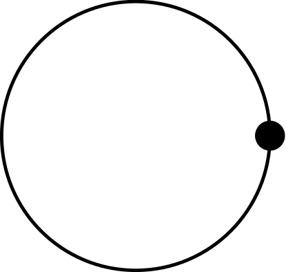
(b)

(c)

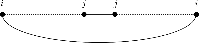
(d)

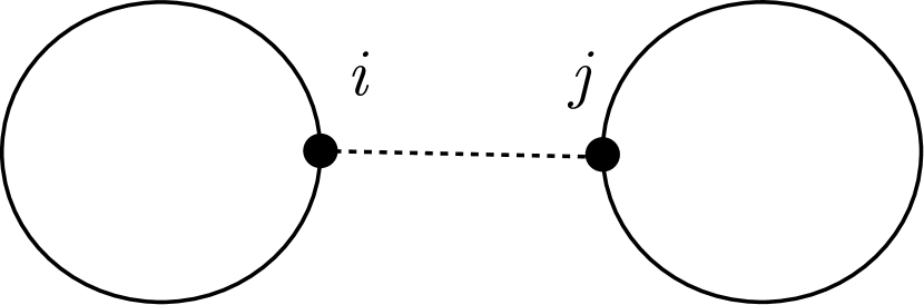
(e)

Figure 2: (a) A visualization of $\rho_{ij}$, which can be regarded as a bridge connecting state $i$ to state $j$. (b) $\Tr(\rho)$ can be obtained from $\rho_{ij}$ by first identifying $i$ and $j$, and then performing a summation over $i=j$. We show it simply by a circle. (c) The product $\rho_{ij}\rho_{ji}$ (no-summation) is shown as the two successive bridges accordingly. (d) Hawking saddle forms one loop and is dominated at initial stages of the evaporation process. (e) Replica saddle forms two loops by gluing the black holes interiors, and is dominated at final stages of the evaporation process.

Figs. 22(d) and 22(e) are topologically different. The first one forms one loop and reproduces Hawking’s calculations, called “Hawking saddle”. However, the second one forms two loops and hence corresponds to some different paths in the context of path integral. It is called “replica saddle”, because the interiors of the black holes are joined together forming a kind of wormhole, called replica wormhole. One would deduce from its topology that it is going to give $(\Tr\rho)^{2}$ (which is unity if the wave function is truly normalized). As the quantity $(\Tr\rho)^{2}-\Tr(\rho^{2})$ is a measure of “purity”, fig. 22(e) leads to a pure final state in the evaporation process. It should be noticed that the Hawking saddle has an exponentially small contribution to the purity in the final stages. Hence it is not going to get the arguments into trouble. Moreover, there are more replicas present in the calculations, $n=3,\ldots$. Although they contribute to the calculations, they do not affect our qualitative arguments about unitarity of the evaporation process (beneficial discussions are presented in Kibe2022 ). As a matter of fact, the entanglement entropy is mostly given by the Hawking saddle at the initial stages and by the replica saddle at the final ones. Thus the evaporation process is unitary. Here we have only stated some results of the calculations which would be found in detail in some works such as Penington2022 ; Almheiri2020 .

We made use of purity instead of entanglement entropy in studying unitarity of the evaporation process. The same results will be obtained if one makes use of entanglement entropy. However, it is a bit tricky because of the required analytic continuation of $n$. As the replica saddle is joining the black holes interiors together, we face with a difficulty in taking the limit $n\rightarrow 1$. In fact, a cut is needed in going from $n=2$ to $n=1$, as is shown in fig. 3. Such a cut cannot be regarded as a fine operation. This fact would explain the reason for using replica trick: The replica saddle might be difficult to see in the case of $n$ exactly 1, hence one would miss it as Hawking did!

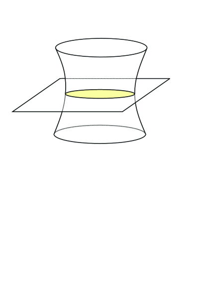
Figure 3: Replica saddle glues the black holes interiors. So a cut is needed when taking the limit $n\rightarrow 1$, which is shown by the cutting surface.

It would be fruitful to summarize this subsection: Replica trick is a mathematical tool which can be used to calculate entanglement entropy of a system. For the special case of an evaporating black hole, this tool will help us to consider all the paths contributing to the respective path integral. To be more specific, the particles that are leaving the black hole have some entanglement with it. This can be regarded as the first order term in the calculation of entanglement entropy, called Hawking saddle. The particles have also some entanglement with those that have left the black hole before. The latter can be seen if one considers higher order terms, or equivalently, $n=2,3,\ldots$ replicas. One should at least consider $n=2$ replicas to realize that the evaporation process preserves unitarity.

3 Shape dependence of entanglement entropy

Entanglement entropy plays a key role in understanding quantum field theories and quantum gravity Nomura2018 ; Faulkner2022 . As it represents the amount of entanglement between a system and its environment, it depends on the shape of the boundary of the system. Hence one may think about its variations (first, second, etc) with respect to boundary variations. Specifically its second variation, called entanglement density, is very interesting due to its relationship with energy density and is studied in some special cases Leichenauer2018 ; Faulkner2016 ; Lewkowycz2018 ; Rosenhaus2015 . In this section, we derive some consistency requirements for entanglement entropy variations with respect to some boundary deformations. Such consistency requirements help us to obtain relations, among which some would be very fruitful in obtaining a true curve for an evaporating black hole—Page curve. As it is discussed in the following subsection, the relations might be regarded as some mathematical identities resulting from the fact that the entanglement entropy is a well-defined functional of the boundary.

3.1 Consistency constraints on entanglement entropy variation

In this subsection, we obtain relations among different orders of entanglement entropy variation with respect to some boundary deformation. To begin with, we consider a system specified by its boundary, $\chi^{\mu}$. The system has some entanglement entropy $S$, which depends on the boundary of the system $\chi$, as well as the matter fields it contains. If the boundary deforms by $\delta\chi$, the entanglement entropy varies which is shown by $\delta S(\chi,\delta\chi)$. One would expand it in terms of the second argument, $\delta\chi$, as follows

$$\delta S(\chi,\delta\chi)=\sum_{i=1}^{\infty}\int\delta\chi_{\mu_{1}}(x_{1})\delta\chi_{\mu_{2}}(x_{2})\cdots\delta\chi_{\mu_{i}}(x_{i})I_{i}^{\mu_{1}\mu_{2}\cdots\mu_{i}}\left[\chi\right](x_{1},x_{2},\ldots,x_{i}).$$ (10)

The coefficients of expansion, $I$’s, depend on the initial boundary $\chi$ (written in brackets), and the points through the boundary and matter fields (written in parentheses). The boundary deformation leads to addition/subtraction of points to/from the system. Moreover, every set of $n$ points has an entanglement entropy and hence contribute to $\delta S$. So we included every order of the boundary deformation—$(\delta\chi)^{n},n=1,2,\ldots$—in the above relation through the summation. However, the zeroth order term is omitted due to the fact that there is no entanglement entropy variation without boundary deformation. In addition, the integrations are taken over the boundary so that all the points are taken into account. Contractions are also assumed over the repeated indices, $\mu$’s. Hence the deformations are considered in all the directions.

Nothing should change if we first send $\chi$ to $\chi+\delta\chi$ and then send it back to its initial form $\chi$, i.e.,

$$\delta S(\chi,\delta\chi)+\delta S(\chi+\delta\chi,-\delta\chi)=0.$$ (11)

The identity (11) is a consistency condition which should be satisfied for the entanglement entropy to be well-defined. Otherwise, $S(\chi)$ might be multi-valued for a system specified by a unique boundary $\chi$. The consistency condition, Eq. (11), can be transformed into relations among the integrands of Eq. (10), $I$’s. To do so, we first write expansions for $\delta S(\chi,\delta\chi)$ and $\delta S(\chi+\delta\chi,-\delta\chi)$ as of Eq. (10)

$$\begin{split}\delta S(\chi,\delta\chi)=&\sum_{i=1}^{\infty}\int\delta\chi_{\mu_{1}}(x_{1})\cdots\delta\chi_{\mu_{i}}(x_{i})I_{i}^{\mu_{1}\cdots\mu_{i}}\left[\chi\right](x_{1},\ldots,x_{i}),\\ \delta S(\chi+\delta\chi,-\delta\chi)=&\sum_{i=1}^{\infty}\left(-1\right)^{i}\int\delta\chi_{\mu_{1}}(x_{1})\cdots\delta\chi_{\mu_{i}}(x_{i})I_{i}^{\mu_{1}\cdots\mu_{i}}\left[\chi+\delta\chi\right](x_{1},\ldots,x_{i}).\end{split}$$ (12)

Then we expand $I[\chi+\delta\chi]$ around $\chi$

$$I\left[\chi+\delta\chi\right]=\sum_{j=0}^{\infty}\int\frac{1}{j!}\frac{\partial^{j}I}{\partial\chi_{\mu_{1}}(x_{1})\partial\chi_{\mu_{2}}(x_{2})\cdots\partial\chi_{\mu_{j}}(x_{j})}\left[\chi\right]\delta\chi_{\mu_{1}}(x_{1})\delta\chi_{\mu_{2}}(x_{2})\cdots\delta\chi_{\mu_{j}}(x_{j}).$$ (13)

The derivatives in the above expansion are functional derivatives and people mostly use $\delta$ for them. However, we made use of $\partial$ to prevent confusion with the $\delta$’s used for entropy variations and boundary deformations. Finally we request the identity to be held independently for each order of boundary deformation and in each set of points due to the arbitrariness of deformation, $\delta\chi(x)$. So we collect coefficients of $\delta\chi_{\mu_{1}}(x_{1})\cdots\delta\chi_{\mu_{m}}(x_{m})$ to obtain the following set of relations

$$\left(1+(-1)^{m}\right)I_{m}^{\mu_{1}\cdots\mu_{m}}(x_{1},\ldots,x_{m})=\sum_{l=1}^{m-1}\frac{(-1)^{l+1}}{(m-l)!}\frac{\partial^{m-l}I_{l}^{\mu_{1}\cdots\mu_{l}}(x_{1},\ldots,x_{l})}{\partial\chi_{\mu_{l+1}}(x_{l+1})\cdots\partial\chi_{\mu_{m}}(x_{m})},$$ (14)

for $m=1,2,\ldots$. A relation that we will mostly use in this work can be obtained from Eq. (14) by setting $m=2$,

$$2I_{2}^{\mu\nu}(x_{1},x_{2})=\frac{\partial I_{1}^{\mu}(x_{1})}{\partial\chi_{\nu}(x_{2})}.$$ (15)

From now on, we drop the $\mu_{i}$ indices and the $x_{i}$ dependencies for briefness.

The left hand side of Eq. (14) vanishes for odd values of $m$. Hence, it does not express any odd-order $I$ in terms of the derivative terms. Nevertheless, such expressions would be found by using some other consistency requirement: Let first deforming the boundary $\chi$ into $\chi+\delta\chi$, then sending $\chi+\delta\chi$ to $\chi+2\delta\chi$, and finally turning it back to its initial form, $\chi$. As before, one would expect that nothing should change under these three successive transformations, i.e.,

$$\delta S(\chi,\delta\chi)+\delta S(\chi+\delta\chi,\delta\chi)+\delta S(\chi+2\delta\chi,-2\delta\chi)=0.$$ (16)

This consistency condition leads to relations, among which some might not be independent of those of Eq. (14)—As an example, it gives Eq. (15) again. Desirably, some expressions would be obtained for some odd-order $I$’s in terms of the derivative terms, such as

$$6I_{3}=-\frac{7}{2}\cdot\frac{\partial^{2}I_{1}}{\partial\chi^{2}}+9\cdot\frac{\partial I_{2}}{\partial\chi},$$ (17)

which can also be combined with the $m=3$ case of Eq. (14) to obtain

$$6I_{3}=2\cdot\frac{\partial I_{2}}{\partial\chi}=\frac{\partial^{2}I_{1}}{\partial\chi^{2}}.$$ (18)

Following Eqs. (11) and (16), more consistency identities can be written for entanglement entropy variations with respect to some boundary deformations. In general, one would expect

$$\delta S(\chi,\delta\chi)+\delta S(\chi+\delta\chi,\delta\chi)+\cdots+\delta S(\chi+(n-1)\delta\chi,\delta\chi)+\delta S(\chi+n\delta\chi,-n\delta\chi)=0,$$ (19)

for $n=1,2,\ldots$. Again one can transform the consistency identities into relations among $I$’s, following the steps made in the case of $n=1$. As stated in the case of $n=2$, not all the relations obtained in this way are independent—Some of them would be reproduced using some others.

3.2 An interpretation for $I_{2}$

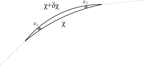
Figure 4: A boundary deformation of a system is shown. The two segments specified by gray squares have a mutual entanglement entropy, which is not going to change the entanglement entropy of the system. This mutual entanglement, however, is considered two times through the first order terms, $I_{1}$’s. The $I_{2}$ terms, inevitably, should cancel these over-calculations.

Let us focus on fig. 4 to find an interpretation for $I_{2}$ in Eq. (10). The boundary is changed from $\chi$ to $\chi+\delta\chi$ so that the system is enlarged. The specified segments (shown by gray squares) participate in $\delta S$ through

$$\begin{split}\left.\delta S\right|_{x_{1}x_{2}}=\;&I_{1}^{\mu}(x_{1})\delta\chi_{\mu}(x_{1})+I_{1}^{\mu}(x_{2})\delta\chi_{\mu}(x_{2})\\ &+I_{2}^{\mu\nu}(x_{1},x_{2})\delta\chi_{\mu}(x_{1})\delta\chi_{\nu}(x_{2})+I_{2}^{\mu\nu}(x_{2},x_{1})\delta\chi_{\mu}(x_{2})\delta\chi_{\nu}(x_{1})+\cdots.\end{split}$$ (20)

The $I_{1}$ terms are standing to take the entanglement entropy variation at the first order. So they are adding the entanglement entropy of each segment with outside (environment), while subtracting the entanglement entropy of that segment with inside (system). However, each couple of segments added to the system has a mutual entanglement entropy which is not going to change the entanglement entropy of the system, but is added to $\delta S$ for two times through $I_{1}(x_{1})$ and $I_{1}(x_{2})$. This mutual entanglement entropy is proportional to both $\delta\chi(x_{1})$ and $\delta\chi(x_{2})$, hence it is proportional to the product $\delta\chi(x_{1})\delta\chi(x_{2})$. Therefore, a modification should occur in the second order to cancel these over-calculations. In other words, the $I_{2}$ terms are standing to cancel the added mutual entanglement entropies, i.e.,

$$\begin{split}\left(I_{2}^{\mu\nu}(x_{1},x_{2})+I_{2}^{\nu\mu}(x_{2},x_{1})\right)&\delta\chi_{\mu}(x_{1})\delta\chi_{\nu}(x_{2})=\\ &-2\times\left(\text{mutual entanglement entropy of segments 1 \& 2}\right).\end{split}$$ (21)

The expression at the left hand side of the above equation can be written in a more brief manner using the following definition

$$\text{Sym}\{I_{2}^{\mu\nu}(x_{1},x_{2})\}:=\frac{1}{2}\left(I_{2}^{\mu\nu}(x_{1},x_{2})+I_{2}^{\nu\mu}(x_{2},x_{1})\right).$$ (22)

Thus we can simply write

$$\text{Sym}\{I_{2}^{\mu\nu}(x_{1},x_{2})\}\delta\chi_{\mu}(x_{1})\delta\chi_{\nu}(x_{2})=-\left(\text{mutual entanglement entropy of segments 1 \& 2}\right),$$ (23)

which is the desired interpretation for $I_{2}$.

3.3 Interpreting the higher order terms, $I_{3}$ etc

To complete the discussion, we want to note that there are more over-calculations present in the first order terms, to be canceled with including higher order terms, $I_{3}$ etc. To clarify, let consider three segments added to the system simultaneously, and write $\delta S|{x_{1}x_{2}x_{3}}$, like what we did in Eq. (20). This time we write the terms up to the third order explicitly, i.e.,

$$\begin{split}\left.\delta S\right|_{x_{1}x_{2}x_{3}}=&I_{1}(x_{1})\delta\chi(x_{1})+I_{1}(x_{2})\delta\chi(x_{2})+I_{1}(x_{3})\delta\chi(x_{3})\\ +&2I_{2}(x_{1},x_{2})\delta\chi(x_{1})\delta\chi(x_{2})+2I_{2}(x_{2},x_{3})\delta\chi(x_{2})\delta\chi(x_{3})+2I_{2}(x_{1},x_{3})\delta\chi(x_{1})\delta\chi(x_{3})\\ +&\left(3!\right)I_{3}(x_{1},x_{2},x_{3})\delta\chi(x_{1})\delta\chi(x_{2})\delta\chi(x_{3})+\cdots,\end{split}$$ (24)

where the coefficients $I_{2}$ and $I_{3}$ are assumed to be symmetric with respect to their arguments, like what we did in Eq. (22). It is possible to have a non-zero tripartite entanglement among the segments. In such a situation, one is adding this tripartite entanglement entropy three times through $I_{1}$’s in the first line of the above equation. The $I_{3}$ terms should cancel these over-calculations, i.e.,

$$\begin{split}\left(3!\right)I_{3}(x_{1},x_{2},x_{3})&\delta\chi(x_{1})\delta\chi(x_{2})\delta\chi(x_{3})=\\ -3\times&\left(\text{tripartite entanglement entropy of segments 1,2 and 3}\right).\end{split}$$ (25)

Continuing this procedure, one can deduce in general that

$$\begin{split}\text{Sym}\{I_{n}(x_{1},x_{2},\ldots,x_{n})\}&\delta\chi(x_{1})\delta\chi(x_{2})\cdots\delta\chi(x_{n})=\\ &-\frac{n}{n!}\times\left(n\text{-partite entanglement entropy of segments }1,2,\ldots,n\right),\end{split}$$ (26)

which is a generalization of Eq. (23) for $n=2,\ldots$.

3.4 An example

One can rummage Eq. (14) to find some useful results. As an example, we consider two systems with entangling surfaces $\chi_{0}$ and $\chi_{0}+\Delta\chi$ respectively, where $\chi_{0}$ is a planar surface and $\Delta\chi$ may differ from point to point. We label the systems by 1 and 2 as shown in fig. 5. The following is an expansion for the entanglement entropy variation of the system 2 under some boundary deformation $\delta\chi$

Figure 5: A part of the boundaries of two systems and their corresponding deformations are shown. The systems are labeled by 1 and 2 with the system 1 having an initially planar boundary. The system 2 has a boundary different from that of the system 1 by amount of $\Delta\chi$, which can differ from point to point.

$$\delta S^{(2)}=\delta S(\chi_{0}+\Delta\chi,\delta\chi)=\int I_{1}^{(2)\,\mu}(x_{1})\delta\chi_{\mu}(x_{1})+\int I_{2}^{(2)\,\mu\nu}(x_{1},x_{2})\delta\chi_{\mu}(x_{1})\delta\chi_{\nu}(x_{2})+\cdots,$$ (27)

where the superscript index $(2)$ refers to the system 2. An analogous expansion can also be written for the system 1, i.e., for $\delta S^{(1)}=\delta S(\chi_{0},\delta\chi)$.

One can expand the coefficients of Eq. (27), $I^{(2)}$’s, around $\chi_{0}$ to find a relation between the two entanglement entropy variations: $\delta S^{(1)}$ and $\delta S^{(2)}$, i.e.,

$$\begin{split}\delta S^{(2)}=&\int I_{1}^{(1)\,\mu}(x_{1})\delta\chi_{\mu}(x_{1})+\int\frac{\partial I_{1}^{(1)\,\mu}(x_{1})}{\partial\chi_{\nu}(x_{2})}\delta\chi_{\mu}(x_{1})\Delta\chi_{\nu}(x_{2})+\cdots\\ &+\int I_{2}^{(1)\,\mu\nu}(x_{1},x_{2})\delta\chi_{\mu}(x_{1})\delta\chi_{\nu}(x_{2})+\cdots\\ &+\cdots,\end{split}$$ (28)

where the superscript index $(1)$ refers to expansion around the planar surface $\chi_{0}$. Inserting $\partial I_{1}^{(1)}/\partial\chi$ from Eq. (15) and considering the special case of $\Delta\chi=n\delta\chi$, we have

$$\begin{split}\delta S^{(2)}&=\delta S(\chi_{0}+n\delta\chi,\delta\chi)\\ &=\int I_{1}^{(1)\,\mu}(x_{1})\delta\chi_{\mu}(x_{1})+\left(2n+1\right)\int I_{2}^{(1)\,\mu\nu}(x_{1},x_{2})\delta\chi_{\mu}(x_{1})\delta\chi_{\nu}(x_{2})+\cdots.\end{split}$$ (29)

Dividing it by $\delta S^{(1)}$, we have

$$\begin{split}\frac{\delta S^{(2)}}{\delta S^{(1)}}&=\frac{\delta S(\chi_{0}+n\delta\chi,\delta\chi)}{\delta S(\chi_{0},\delta\chi)}\\ &=\frac{\int I_{1}^{(1)\,\mu}(x_{1})\delta\chi_{\mu}(x_{1})+\left(2n+1\right)\int I_{2}^{(1)\,\mu\nu}(x_{1},x_{2})\delta\chi_{\mu}(x_{1})\delta\chi_{\nu}(x_{2})+\cdots}{\int I_{1}^{(1)\,\mu}(x_{1})\delta\chi_{\mu}(x_{1})+\int I_{2}^{(1)\,\mu\nu}(x_{1},x_{2})\delta\chi_{\mu}(x_{1})\delta\chi_{\nu}(x_{2})+\cdots},\end{split}$$ (30)

where we made use of Eq. (29) for $\delta S^{(1)}$ by setting $n=0$. For some special cases, such as a CFT in the vacuum state, we have (see Allais2015 ; Faulkner2016 for proof)

$$I_{1}^{(1)\,\mu}(x)=0.$$ (31)

In such cases, the leading term of the right hand side of Eq. (30) is

$$\frac{\delta S^{(2)}}{\delta S^{(1)}}=\frac{\delta S(\chi_{0}+n\delta\chi,\delta\chi)}{\delta S(\chi_{0},\delta\chi)}=(1+2n)+\mathcal{O}(\delta\chi).$$ (32)

This leading term is quiet simple and independent of any details of the systems. This occurred thanks to Eq. (31), which is a result of the very restrictive assumption of a CFT in the vacuum state. Higher order terms, however, will depend on the details through the coefficients, $I^{(1)}$’s. An expression is obtained for $\delta S^{(1)}$ in Rosenhaus2014 ; by using which, one can also obtain an expression for $\delta S^{(2)}$ through Eq. (30). It should be noticed that for a CFT, the planar entangling surface can be converted to a ball-shaped one through a conformal map. Hence the relations can also be converted to those of a ball-shaped entangling surface.

The obtained result, Eq. (30), can be generalized to include any small $\Delta\chi$ parallel to $\delta\chi$. First let us define $m(x)$ through

$$\Delta\chi_{\mu}(x)=m(x)\delta\chi_{\mu}(x).$$ (33)

Then we substitute $n\delta\chi$ in Eq. (30) with the above expression for $\Delta\chi$, still keeping $I_{1}^{(1)}$ zero. Finally we expand $m(x)$ around its maximum, namely $m(x_{0})$, and only keep the leading term to obtain

$$\frac{\delta S(\chi_{0}+m(x)\delta\chi,\delta\chi)}{\delta S(\chi_{0},\delta\chi)}=\left(1+2m(x_{0})\right)+\mathcal{O}(\delta\chi).$$ (34)

One can geometrically interpret $m(x_{0})$ as the maximum number of $\delta\chi$’s that can be placed in $\Delta\chi$ at $x=x_{0}$. Again, the higher order terms neglected depend on the details of the systems through the coefficients, $I$’s.

We summarize this subsection as: For two systems with planar and near-planar entangling surfaces $\chi_{0}$ and $\chi_{0}+m(x)\delta\chi$, which are described by a CFT in the vacuum state, we have

$$\delta S(\chi_{0}+m(x)\delta\chi,\delta\chi)\approx\left(1+2\times\mathrm{Max}_{x}\left\{m(x)\right\}\right)\delta S(\chi_{0},\delta\chi).$$ (35)

4 Entanglement entropy of a radiating black hole and the Page curve

In this section, we consider a gravitation theory in (3+1)-dimensions, which is holographically dual to a field theory in (2+1)-dimensions, and respects the bound $S\leq A/4G$, to obtain the entanglement entropy of an evaporating Schwarzschild black hole. To begin with, we consider the holographic dual of the black hole, which is a disk of radius $r_{1}$ in two spatial dimensions called $\mathcal{A}$. The entanglement entropy of $\mathcal{A}$ depends on its radius, $r_{1}$, as well as on the details of the field theory that describes it. As discussed in Sec. 1, we do not specify the details of the field theory here. Rather, we make use of the holographic assumptions alongside the consistency relations of Sec. 3, to obtain a curve for the entanglement entropy of the black hole. This curve will be found to be similar to the Page curve in its general shape. Nonetheless, some model-dependent modifications would occur, one of which is explained in subsection 4.1.

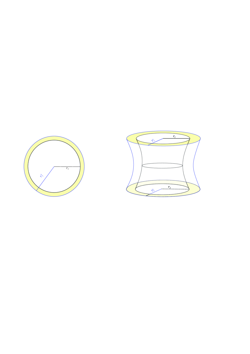
Figure 6: Left: A (2+1)-dimensional disk is shown in two spatial dimensions, which is holographically dual to a (3+1)-dimensional black hole. The yellow-shaded region is added to the disk by a radius variation, which leads to some entanglement entropy variation. Right: $n=2$ replicas are shown, although with different radii! The yellow-shaded regions represent radii variations which lead to some variation of the entanglement entropy of the system. The connecting curves (wormhole) represent some entanglement between the disks in the sprite of ER=EPR.

Let start the procedure by considering the disk $\mathcal{A}$ and variating its radius from $r_{1}$ to $r_{1}^{\prime}=r_{1}+\delta r_{1}$, fig. 6, left. The variation of the entanglement entropy takes the form

$$\delta S_{\mathcal{A}}=I_{1}(r_{1})\delta r_{1},$$ (36)

where $I_{1}$ contains the unspecified details of the field theory. The points added to $\mathcal{A}$, shown by yellow in the figure, have some entanglement with both $\mathcal{A}$ and the environment. Thus $I_{1}(r_{1})\delta r_{1}$ contains the entanglement entropies of the points with the environment and $\mathcal{A}$, with positive and negative signs respectively. Hence it should be proportional to the number of the added points, or equivalently, to the added area, i.e.,

$$I_{1}(r_{1})\delta r_{1}=cr_{1}\delta r_{1},$$ (37)

where we absorbed a factor of $2\pi$ in $c$. Moreover, $c$ contains information about the field theory; hence it depends on $r_{1}$ in general. So we would expand it in terms of $r_{1}$, or equivalently, make use of the replica trick according to the discussions passed in Sec. 2.1.

Let consider $n=2$ replicas and label them by 1 and 2, as in fig. 6 right. We take the radii of the disks to be different at first. However, we set them equal after we found a proper expression for the entanglement entropy variation, $\delta S^{(n=2)}$. This would be considered as a trick for obtaining some relations much easier. The entanglement entropy variation due to the radii variations takes the general form

$$\delta S^{(n=2)}=I_{1}(r_{1};r_{2})\delta r_{1}+I_{1}(r_{2};r_{1})\delta r_{2}+2I_{2}(r_{1},r_{2})\delta r_{1}\delta r_{2},$$ (38)

where $r^{\prime}_{1}$ and $r^{\prime}_{2}$ in the figure are substituted by $r_{1}+\delta r_{1}$ and $r_{2}+\delta r_{2}$ respectively. The first (second) term is standing to take the entanglement entropy variation between the disk 1 (2), shown by darker (lighter) yellow, with the environment into account; while the $I_{2}$ term (symmetric under $r_{1}\leftrightarrow r_{2}$) is standing to take the entanglement entropy variation between the disks, 1 and 2, into account. The connecting curves in fig. 6, right, are referring to such an entanglement in the spirit of ER=EPR. We have separated $r_{1}$ and $r_{2}$ dependence of $I_{1}(r_{1};r_{2})$ (or $I_{1}(r_{2};r_{1})$) by “;” to emphasize that: Although the term $I_{1}(r_{1};r_{2})\delta r_{1}$ is standing for the entanglement change of the disk 1 and the environment, it implicitly depends on the value of $r_{2}$ due to the presence of some entanglement between the disks, 1 and 2. One can deduce, as in Eq. (37), that

$$I_{1}(r_{1};r_{2})\delta r_{1}=\frac{\alpha(r_{2})r_{1}}{G}\delta r_{1},$$ (39)

and

$$I_{1}(r_{2};r_{1})\delta r_{2}=\frac{\alpha(r_{1})r_{2}}{G}\delta r_{2},$$ (40)

where $G$ is the Newton’s constant in (3+1) dimensions, inserted to make $\alpha$ dimensionless. As one can see, we dropped the dependence of $\alpha$ on the first argument of $I_{1}$ according to the discussion made after Eq. (37). One can also deduce that the $I_{2}(r_{1},r_{2})\delta r_{1}\delta r_{2}$ term should be proportional to both the number of the points added to disk 1 and disk 2; or equivalently, it should be proportional to the multiplication of the areas of the two yellow-shaded regions in fig. 6 right, i.e.,

$$I_{2}(r_{1},r_{2})\delta r_{1}\delta r_{2}=-\frac{\zeta r_{1}r_{2}}{G^{2}}\delta r_{1}\delta r_{2},$$ (41)

where $\zeta$ is a dimensionless constant and positive according to Eq. (23)—The minus sign is inserted to make it positive. Making use of Eq. (15), one can find the following relation between the unknown coefficients, $\alpha$ and $\zeta$

$$\frac{d\alpha(r)}{dr}=-\frac{2\zeta r}{G},$$ (42)

which leads to

$$\alpha(r)=-\frac{\zeta r^{2}}{G}+\gamma,$$ (43)

with $\gamma$ being a dimensionless constant. Now we can write down the entropy variation as

$$\delta S^{(n=2)}=\left(\gamma-\frac{\zeta r_{2}^{2}}{G}\right)\frac{r_{1}}{G}\delta r_{1}-\frac{2\zeta r_{1}r_{2}}{G^{2}}\delta r_{1}\delta r_{2}+\left(\gamma-\frac{\zeta r_{1}^{2}}{G}\right)\frac{r_{2}}{G}\delta r_{2}.$$ (44)

It is an easy task to find an expression for $\delta S_{\mathcal{A}}$. To do so, let look at the terms participating in $\delta S^{(n=2)}$. We have two $I_{1}$ terms which is a direct consequence of having $n=2$ replicas. Moreover, every pair of replicas will lead to a $2I_{2}$ term. Thus returning the $n$-dependence and setting $r_{1}=r_{2}=r$, we have

$$\delta S^{(n=2\rightarrow n)}=n\left(\gamma-\frac{\zeta r^{2}}{G}\right)\frac{r}{G}\delta r-2\binom{n}{2}\frac{\zeta r^{2}}{G^{2}}\delta r^{2},$$ (45)

where the superscript index $(n=2\rightarrow n)$ is indicating that we have obtained the above equation from $n=2$ replicas. There are also other terms participating in $\delta S$ which would be appear when we consider more replicas, $n=3$ etc. Performing the limit $n\rightarrow 1$, the above equation gives

$$\delta S^{(2)}=\delta S_{\mathcal{A}}\approx\left(\gamma-\frac{\zeta r^{2}}{G}\right)\frac{r}{G}\delta r,$$ (46)

where the superscript $(2)$ refers to the fact that we have considered the terms up to $I_{2}$.

It should be noticed that although the term $I_{2}(r_{1},r_{2})\delta r_{1}\delta r_{2}$ disappeared from our calculations in the limit $n\rightarrow 1$, it played an essential role in deriving the above expression for the entanglement entropy variation. The entanglement entropy can easily be obtained from the above equation

$$S^{(2)}(r)=\frac{\gamma r^{2}}{2G}-\frac{\zeta r^{4}}{4G^{2}}.$$ (47)

The two unknown constants $\zeta$ and $\gamma$ would be found by using the following constraints on the dual black hole: i) The entanglement entropy vanishes at $r=r_{0}$—the initial radius of the black hole—which means that the black hole was initially in a pure state, i.e.,

$$S(r=r_{0})=0.$$ (48)

ii) The entanglement entropy will not exceed the Bekenstein-Hawking entropy, $A/4G$—At most, it saturates the bound. Thus we have

$$\text{Max}_{r}\left\{\frac{4GS(r)}{A(r)}\right\}=1.$$ (49)

It is obvious from Eq. (47) that the maximum occurs when $r\rightarrow 0$. Applying these two boundary conditions for $r=0$ and $r=r_{0}$, one obtains $\gamma=2\pi$ and $\zeta=4\pi G/r_{0}^{2}$, hence

$$S^{(2)}(r)=\frac{\pi r^{2}}{G}-\frac{\pi r^{4}}{Gr_{0}^{2}}=\frac{\pi r^{2}}{G}\left(1-\frac{r^{2}}{r_{0}^{2}}\right).$$ (50)

We can easily convert the $r$-dependence of $S$ into the time-dependence. To do so, we would make use of $r=2GM$, with $M$ being mass of the black hole variating by time as given in Page2013

$$M(t)=M_{0}\left(1-\frac{t}{t_{\text{decay}}}\right)^{1/3},$$ (51)

where $M_{0}$ is the initial mass of the black hole and $t_{\text{decay}}$ is the time duration of the evaporation process as measured by an asymptotic observer. Hence we find

$$S^{(2)}(t)=\pi GM_{0}^{2}\left(1-\frac{t}{t_{\text{decay}}}\right)^{2/3}\left[1-\left(1-\frac{t}{t_{\text{decay}}}\right)^{2/3}\right].$$ (52)

In the limit $r\ll r_{0}$, or equivalently $t\lesssim t_{\text{decay}}$, Eqs. (50) and (52) give

$$S^{(2)}\left(r\ll r_{0}\right)\approx\frac{\pi r^{2}}{G},\qquad S^{(2)}\left(t\lesssim t_{\text{decay}}\right)\approx 4\pi GM_{0}^{2}\left(1-\frac{t}{t_{\text{decay}}}\right)^{2/3},$$ (53)

the left of which is the Bekenstein-Hawking entropy formula $S=A/4G$. In the other limit of interest $r\lesssim r_{0}$, or equivalently $t\ll t_{\text{decay}}$, we have

$$S^{(2)}\left(r\lesssim r_{0}\right)\approx\frac{2\pi}{G}r_{0}\left(r_{0}-r\right),\qquad S^{(2)}\left(t\ll t_{\text{decay}}\right)\approx\frac{8\pi GM_{0}^{2}}{3}\frac{t}{t_{\text{decay}}}.$$ (54)

One can compare the obtained results with those of Page Page2013

$$\begin{split}S_{\text{Page}}(t)=4\pi G\beta M_{0}^{2}\left[1-\left(1-\frac{t}{t_{\text{decay}}}\right)^{2/3}\right]&\theta\left(t_{\text{Page}}-t\right)\\ +&4\pi GM_{0}^{2}\left(1-\frac{t}{t_{\text{decay}}}\right)^{2/3}\theta\left(t-t_{\text{Page}}\right),\end{split}$$ (55)

where $\theta$ is the Heaviside step function, $\beta\approx 1.48472$ and

$$t_{\text{Page}}=\left[1-\left(\frac{\beta}{\beta+1}\right)^{3/2}\right]t_{\text{decay}}.$$ (56)

Converting the time-dependence into $r$-dependence via Eq. (51) alongside $M=r/2G$, one obtains

$$S_{\text{Page}}(r)=\frac{\pi\beta}{G}\left(r_{0}^{2}-r^{2}\right)\theta\left(r-r_{\text{Page}}\right)+\frac{\pi}{G}r^{2}\theta\left(r_{\text{Page}}-r\right),$$ (57)

where

$$r_{\text{Page}}=\left(1-\frac{t_{\text{Page}}}{t_{\text{decay}}}\right)^{1/3}r_{0}.$$ (58)

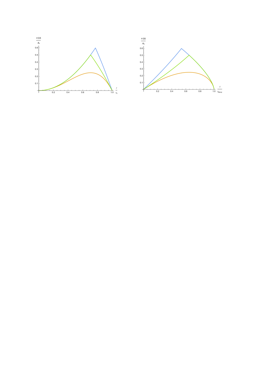
Figure 7: Comparing the obtained results from $n=2$ replicas with those of Page: The orange curves are the results from $n=2$ replicas (Eqs. (50) and (52)); while the blue curves are those of Page (Eqs. (55) and (57)). The green curves are the two limiting behaviors of the orange curves (Eqs. (53) and (54)) extrapolated to the inner region to intersect each other.

The obtained results Eqs. (50) and (52), and those of Page Eqs. (55) and (57) are shown in fig. 7 by orange and blue respectively. As discussed in Sec. 1, the Page curve is obtained by considering the thermodynamic entropies of the radiation and the black hole and switching between them (as shown in fig. 1). Hence we have extrapolated the two limiting behaviors of Eqs. (50) and (52) (which are given by Eqs. (53) and (54)) by green, to compare with the results of Page. As can be seen, they are the same for small to medium values of $r$, or equivalently, for medium to large values of time. Some discrepancies are apparent in the middle points of the diagrams. However, when considering $n=3$ replicas a modification occurs such that the curves (blue and green) may become identical. Such a possibility will be worked out in subsection 4.1. The following are important points obtained from the comparison:

• The most important feature of the Page curve is: It vanishes at both the start point and the end point (time or radius), which is necessary for the evaporation process to be unitary. However, it seems that such a desired behavior can be regarded as a direct consequence of the holographic assumptions made—independent of the details of the gravitation theory such as its field equations.

• The Page curve has a singular (breaking) point which, as discussed in Sec. 1, results from the switching between the thermodynamic entropies of the black hole and the radiation. Thus the discrepancies between the smooth curves (fig. 7, orange) and those of Page (fig. 7, blue) in the middle points are mostly due to the presence of such a point and is almost unavoidable. It is worth noting that one would expect such a singular point to be avoided when deriving the entanglement entropy using a well-behaved manner.

One can think of the time in our results that is equivalent to the Page time—namely $t_{*}$. As there are no breaking points, it can be introduced as the time when the entropy takes its maximum value. Such a time is reported in Table 1 for both cases of considering $n=2$ and $n=3$ replicas.

According to the Hawking pair creation process, the quantum state of the radiation is treated as purely thermal prior to the Page time. However, as the obtained curve (fig. 7, orange) lies below the Page curve (fig. 7, blue), one would conclude that the radiation has more information content. The difference of the maximum entropy values for the Page curve and for the obtained curve, reported in Table 1, can be regarded as a measure of such additional information. Discussions are presented in Kudler-Flam2022 on this subject.

Table 1: The location and height of the maximum points are stated in curves $S_{\text{Page}}(t)$, $S^{(2)}(t)$ and $S^{(3)}(t)$. The quantity $(S_{\text{Page}}(t)-S(t))/S_{\text{Page}}(t)$, for any time prior to the Page time, can be regarded as the amount of additional information about the quantum state of the black hole that is stored in the radiation. This quantity is also stated for the curves in their maxima.

	Value ($\#/t_{\text{decay}}$)	Entropy ($S/4\pi GM_{0}^{2}$)	$(S_{\text{Page}}-S)/S_{\text{Page}}$
$t_{\text{Page}}$	$0.54$	$0.60$	0
$t_{*}^{(2)}$	$0.65$	$0.25$	$0.58$
$t_{*}^{(3)}$	$0.59$	$0.31$	$0.48$

4.1 Considering $n=3$ replicas

As mentioned earlier in this section, the details of the gravitation theory, such as its field equations, affect our calculations by some higher order terms ($\mathcal{O}(r^{6})$) that are coming into account when we consider more replicas ($I_{3}$, etc). As the first correction to Eq. (50), let consider $n=3$ replicas. In this situation a term $I_{3}$ corresponding to some tripartite entanglement should be included, which through the same arguments as of $I_{1}$ and $I_{2}$ should be of the form

$$I_{3}(r_{1},r_{2},r_{3})\delta r_{1}\delta r_{2}\delta r_{3}=-\frac{\eta r_{1}r_{2}r_{3}}{6G^{3}}\delta r_{1}\delta r_{2}\delta r_{3},$$ (59)

with $\eta$ being a positive dimensionless constant. Such a term will give an $r^{6}$ correction to Eq. (47). Hence the modified equation becomes

$$S^{(3)}(r)=\frac{\gamma^{(3)}r^{2}}{2G}-\frac{\zeta^{(3)}r^{4}}{4G^{2}}-\frac{\eta r^{6}}{6G^{3}},$$ (60)

where the superscript $(3)$ refers to the fact that we have considered the terms up to $I_{3}$.

One would expect the constant $\eta$ to be computed directly from the gravitation theory or its dual field theory. However, we want just to show that it is possible for such a term to modify our results to be in more agreement with those of Page, specially for $r\lesssim r_{0}$, or equivalently for $t\ll t_{\text{decay}}$. The three constants of Eq. (60) should be determined by three boundary conditions. We have two of them (as before) and assume that the third one is enforcing the $r\lesssim r_{0}$ limiting behavior of the entanglement entropy to be matched with the Page’s result. Hence the boundary conditions are

$$\text{Max}_{r}\left\{\frac{4GS(r)}{A(r)}\right\}=1,\qquad S(r=r_{0})=0,\qquad\left.\frac{dS(r)}{dr}\right|_{r\rightarrow r_{0}}=-\frac{2\pi\beta}{G}r_{0},$$ (61)

which result in

$$\gamma^{(3)}=2\pi=\gamma,\qquad\zeta^{(3)}=\frac{4\pi G(2-\beta)}{r_{0}^{2}},\qquad\eta=\frac{6\pi G^{2}(\beta-1)}{r_{0}^{4}},$$ (62)

that give

$$S^{(3)}(r)=\frac{\pi r^{2}}{G}-(2-\beta)\frac{\pi r^{4}}{Gr_{0}^{2}}-(\beta-1)\frac{\pi r^{6}}{Gr_{0}^{4}}.$$ (63)

Replacing from Eq. (51), we find the following expression for $S^{(3)}(t)$

$$S^{(3)}(t)=4\pi GM_{0}^{2}\left[\left(1-\frac{t}{t_{\text{decay}}}\right)^{2/3}-(2-\beta)\left(1-\frac{t}{t_{\text{decay}}}\right)^{4/3}-(\beta-1)\left(1-\frac{t}{t_{\text{decay}}}\right)^{2}\right].$$ (64)

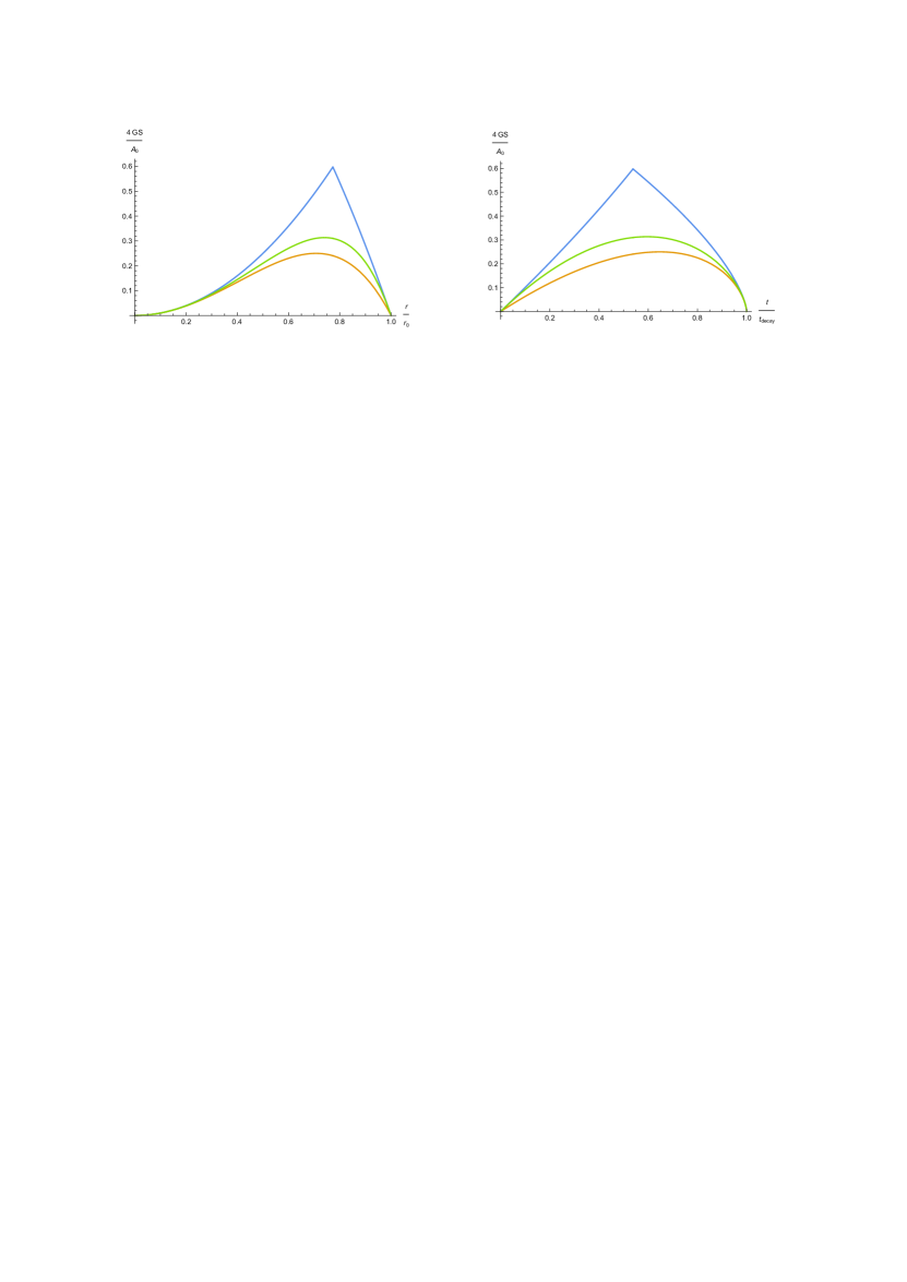
Figure 8: Comparing the obtained results from $n=2$ and $n=3$ replicas with those of Page: The orange curves are the results from $n=2$ replicas (Eqs. (50) and (52)); while the green curves are those from $n=3$ replicas (Eqs. (63) and (64)) and the blue curves are the results of Page (Eqs. (55) and (57)). The limiting behaviors of the orange curves are shown in fig. 6, while the limiting behaviors of the green curves coincide the results of Page.

The modification mostly affect our results in the limit $r\lesssim r_{0}$, or equivalently $t\ll t_{\text{decay}}$, as expected. Both $S^{(3)}(r)$ and $S^{(3)}(t)$ are shown in fig. 8 (green) alongside those obtained from $n=2$ replicas (orange) and those of Page (blue) for comparison. The consistency between the results from $n=3$ replicas and those of Page is obvious. Please note that for $\beta=1$ the modified results coincide the old ones. It is worth noting that the modified curves (fig. 8, green) might be considered as smooth versions of the Page curves up to some $\mathcal{O}(r^{8})$, or equivalently $\mathcal{O}((t_{\text{decay}}-t)^{8/3})$, corrections.

Learning from $n=3$ replicas, we can make some general conclusions about the higher order terms coming from the higher replicas. Following Eq. (60), the terms should be of the form

$$-\frac{\theta_{n}r^{2n}}{2nG^{n}},$$ (65)

with $n=4,\ldots$. $\theta_{n}$ is determined by the gravitation theory and is positive according to subsection 3.3. Although we do not have the coefficients, $\theta$’s, it is an easy task to show that the higher order terms are not going to change the general shape of the obtained curves (fig. 8, orange and green): Since these terms are always negative and of the form $r^{2n}$, $\delta S$ will have exactly one root for $0<r<r_{0}$ (a local maximum). Moreover, the limiting behaviors of the curves are uniquely determined by the boundary conditions, Eq. (61). Hence the modifications will preserve the general shape of the curves.

5 Conclusions

In this work we argued that the Page curve is a consequence of holography—independent of the details of the gravitational field equations. In other words, a holographic theory of gravity which respects the bound $S\leq A/4G$ for entanglement entropy, would result in a Page curve for an evaporating black hole. The details of the gravitation theory and its field equations would affect the curve through some shape-preserving modifications. It is obvious from the holographic assumptions that this work is not regarded as a resolution to the black hole information paradox. Nevertheless, it gives a deeper understanding of the role of holography in preserving the information in gravitation theories.

One would expect the entanglement entropy, $S$, of a system to depend on its boundary, $\chi(x)$. Hence it is considered as a functional of the boundary, $S(\chi)$. For the entanglement entropy to be well-defined (single-valued), it should not change under the following transformation: first deforming $\chi$ to $\chi+\delta\chi$, and then turning it back to $\chi$. This gives some quit general constraints on the entanglement entropy which were worked out in this paper. These constraints helped us a lot in obtaining an expression for the entanglement entropy of an evaporating black hole.

The obtained results indicate that the Hawking radiation prior to the Page time contains some information about the quantum state of the black hole. This means that it cannot be regarded as purely thermal, which is in accordance with some other studies, such as Kudler-Flam2022 . Moreover, the amount of information carried by the radiation prior to the Page time is expected to play an important role in a better understanding of the dynamics of black hole evaporation at the quantum level.

References

- (1) S.W. Hawking, Particle creation by black holes, Commun. Math. Phys. 43 (1975) 199.
- (2) D.N. Page, Particle emission rates from a black hole: Massless particles from an uncharged, nonrotating hole, Phys. Rev. D 13 (1976) 198.
- (3) J.D. Bekenstein, Black holes and the second law, Lett. Al Nuovo Cim. Ser. 2 4 (1972) 737.
- (4) J.M. Bardeen, B. Carter and S.W. Hawking, The four laws of black hole mechanics, Commun. Math. Phys. 31 (1973) 161.
- (5) D.N. Page, Hawking radiation and black hole thermodynamics, New J. Phys. 7 (2005) 1 [0409024].
- (6) S.W. Hawking, Breakdown of predictability in gravitational collapse, Phys. Rev. D 14 (1976) 2460.
- (7) D.N. Page, Comment on ”entropy evaporated by a black hole”, Phys. Rev. Lett. 50 (1983) 1013.
- (8) D.N. Page, Information in black hole radiation, Phys. Rev. Lett. 71 (1993) 3743 [9306083].
- (9) D.N. Page, Time Dependence of Hawking Radiation Entropy, J. Cosmol. Astropart. Phys. 2013 (2013) 028 [1301.4995].
- (10) A. Strominger and C. Vafa, Microscopic origin of the Bekenstein-Hawking entropy, Phys. Lett. B 379 (1996) 99.
- (11) G. ’t Hooft, On the quantum structure of a black hole, Nucl. Phys. B 256 (1985) 727.
- (12) M. Srednicki, Entropy and area, Phys. Rev. Lett. 71 (1993) 666.
- (13) L. Bombelli, R.K. Koul, J. Lee and R.D. Sorkin, Quantum source of entropy for black holes, Phys. Rev. D 34 (1986) 373.
- (14) I. Bena, E.J. Martinec, S.D. Mathur and N.P. Warner, Fuzzballs and Microstate Geometries: Black-Hole Structure in String Theory, 2204.13113.
- (15) V. Balasubramanian, A. Lawrence, J.M. Magan and M. Sasieta, Microscopic origin of the entropy of black holes in general relativity, 2212.02447.
- (16) A. Almheiri, T. Hartman, J. Maldacena, E. Shaghoulian and A. Tajdini, The entropy of Hawking radiation, Rev. Mod. Phys. 93 (2021) 035002 [2006.06872].
- (17) A. Almheiri, N. Engelhardt, D. Marolf and H. Maxfield, The entropy of bulk quantum fields and the entanglement wedge of an evaporating black hole, J. High Energy Phys. 2019 (2019) 63 [1905.08762].
- (18) A. Almheiri, T. Hartman, J. Maldacena, E. Shaghoulian and A. Tajdini, Replica Wormholes and the Entropy of Hawking Radiation, J. High Energy Phys. 2020 (2019) 13 [1911.12333].
- (19) A. Almheiri, R. Mahajan, J. Maldacena and Y. Zhao, The Page curve of Hawking radiation from semiclassical geometry, J. High Energy Phys. 2020 (2020) 149 [1908.10996].
- (20) G. Penington, Entanglement wedge reconstruction and the information paradox, J. High Energy Phys. 2020 (2020) 2 [1905.08255].
- (21) S. Ryu and T. Takayanagi, Holographic Derivation of Entanglement Entropy from AdS/CFT, Phys. Rev. Lett. 96 (2006) 181602 [0603001].
- (22) S. Ryu and T. Takayanagi, Aspects of Holographic Entanglement Entropy, J. High Energy Phys. 2006 (2006) 045 [0605073].
- (23) V.E. Hubeny, M. Rangamani and T. Takayanagi, A covariant holographic entanglement entropy proposal, J. High Energy Phys. 2007 (2007) 062 [0705.0016].
- (24) N. Engelhardt and A.C. Wall, Quantum extremal surfaces: holographic entanglement entropy beyond the classical regime, J. High Energy Phys. 2015 (2015) 73 [1408.3203].
- (25) T. Faulkner, A. Lewkowycz and J. Maldacena, Quantum corrections to holographic entanglement entropy, J. High Energy Phys. 2013 (2013) 74 [1307.2892].
- (26) G.t. Hooft, Dimensional Reduction in Quantum Gravity, AIP Conf. Proc. 116 (1993) 1 [9310026].
- (27) J.M. Maldacena, The Large N Limit of Superconformal Field Theories and Supergravity, Int. J. Theor. Phys. 38 (1997) 1113 [9711200].
- (28) E. Witten, Anti de Sitter space and holography, Adv. Theor. Math. Phys. 2 (1998) 253 [9802150].
- (29) M. Rangamani and T. Takayanagi, Holographic Entanglement Entropy, Lect. Notes Phys. 931 (2016) 35 [1609.01287].
- (30) H. Geng, Y. Nomura and H.Y. Sun, Information paradox and its resolution in de Sitter holography, Phys. Rev. D 103 (2021) 126004 [2103.07477].
- (31) I. Aref’eva and I. Volovich, A Note on Islands in Schwarzschild Black Holes, 2110.04233.
- (32) T. Hartman, E. Shaghoulian and A. Strominger, Islands in asymptotically flat 2D gravity, J. High Energy Phys. 2020 (2020) [2004.13857].
- (33) K. Hashimoto, N. Iizuka and Y. Matsuo, Islands in Schwarzschild black holes, J. High Energy Phys. 2020 (2020) [2004.05863].
- (34) X. Wang, R. Li and J. Wang, Page curves for a family of exactly solvable evaporating black holes, Phys. Rev. D 103 (2021) 126026.
- (35) F.F. Gautason, L. Schneiderbauer, W. Sybesma and L. Thorlacius, Page curve for an evaporating black hole, J. High Energy Phys. 2020 (2020) [2004.00598].
- (36) E.E. Flanagan, D. Marolf and R.M. Wald, Proof of Classical Versions of the Bousso Entropy Bound and of the Generalized Second Law, Phys. Rev. D 62 (1999) 084035 [9908070].
- (37) R. Bousso, E.E. Flanagan and D. Marolf, Simple sufficient conditions for the generalized covariant entropy bound, Phys. Rev. D 68 (2003) 064001 [0305149].
- (38) J.D. Bekenstein, How does the Entropy/Information Bound Work?, Found. Phys. 35 (2005) 1805 [0404042].
- (39) H. Casini, Relative entropy and the Bekenstein bound, Class. Quantum Gravity 25 (2008) 205021 [0804.2182].
- (40) Y.-X. Chen and Y. Xiao, The entropy bound for local quantum field theory, Phys. Lett. B 662 (2008) 71 [0705.1414].
- (41) L.P. Horwitz, V.S. Namboothiri, G. Varma K, A. Yahalom, Y. Strauss and J. Levitan, Entropy Bounds: New Insights, Symmetry (Basel). 14 (2022) 3.
- (42) S.B. Giddings, Holography and unitarity, J. High Energy Phys. 2020 (2020) [2004.07843].
- (43) M. Headrick, V.E. Hubeny, A. Lawrence and M. Rangamani, Causality & holographic entanglement entropy, J. High Energy Phys. 2014 (2014) 162 [1408.6300].
- (44) C.-H. Wu and C.-C. Yen, The Expressivity of Classical and Quantum Neural Networks on Entanglement Entropy, 2305.00997.
- (45) T. Kibe, P. Mandayam and A. Mukhopadhyay, Holographic spacetime, black holes and quantum error correcting codes: a review, Eur. Phys. J. C 82 (2022) 1 [2110.14669].
- (46) G. Penington, S.H. Shenker, D. Stanford and Z. Yang, Replica wormholes and the black hole interior, J. High Energy Phys. 2022 (2022) 205 [1911.11977].
- (47) Y. Nomura, P. Rath and N. Salzetta, Spacetime from unentanglement, Phys. Rev. D 97 (2018) 106010 [1711.05263].
- (48) T. Faulkner, T. Hartman, M. Headrick, M. Rangamani and B. Swingle, Snowmass white paper: Quantum information in quantum field theory and quantum gravity, 2203.07117.
- (49) S. Leichenauer, A. Levine and A. Shahbazi-Moghaddam, Energy density from second shape variations of the von Neumann entropy, Phys. Rev. D 98 (2018) 86013.
- (50) T. Faulkner, R.G. Leigh and O. Parrikar, Shape dependence of entanglement entropy in conformal field theories, J. High Energy Phys. 2016 (2016) 1 [1511.05179].
- (51) A. Lewkowycz and O. Parrikar, The Holographic Shape of Entanglement and Einstein’s Equations, J. High Energy Phys. 2018 (2018) 147 [1802.10103].
- (52) V. Rosenhaus and M. Smolkin, Entanglement entropy for relevant and geometric perturbations, J. High Energy Phys. 2015 (2015) [1410.6530].
- (53) A. Allais and M. Mezei, Some results on the shape dependence of entanglement and Rényi entropies, Phys. Rev. D 91 (2015) 046002 [1407.7249].
- (54) V. Rosenhaus and M. Smolkin, Entanglement entropy: a perturbative calculation, J. High Energy Phys. 2014 (2014) [1403.3733].
- (55) J. Kudler-Flam and Y. Kusuki, On Quantum Information Before the Page Time, 2212.06839.