Privacy-aware Gaussian Process Regression

Abstract

We propose the first theoretical and methodological framework for Gaussian process regression subject to privacy constraints. The proposed method can be used when a data owner is unwilling to share a high-fidelity supervised learning model built from their data with the public due to privacy concerns. The key idea of the proposed method is to add synthetic noise to the data until the predictive variance of the Gaussian process model reaches a prespecified privacy level. The optimal covariance matrix of the synthetic noise is formulated in terms of semi-definite programming. We also introduce the formulation of privacy-aware solutions under continuous privacy constraints using kernel-based approaches, and study their theoretical properties. The proposed method is illustrated by considering a model that tracks the trajectories of satellites.

1 Introduction

This work aims to present a privacy-aware supervised machine learning model. At a high level, a supervised model can be regarded as a mapping from the input space to the output space. In a traditional supervised learning paradigm, the objective is to build a supervised model from the data, with the goal of minimizing its prediction error. With the widespread use of machine learning in various industries, businesses, public sectors, and other fields, data security and privacy protection have become pressing issues that require immediate solutions.

In this article, we discuss data privacy issues in a particular scenario. A data owner intends to release a machine learning model, built using their data, to the public. However, the owner wishes to impose limitations on the prediction accuracy of the released machine learning model, as disclosing a model with the highest possible accuracy could result in private data leakage, security risks, or loss of business interests. At the same time, if the accuracy is deliberately lowered too much, the model will lose its usefulness. Hence, the owner must strike a balance between the utility and privacy of the model.

Despite the rich literature in both machine learning and data privacy domains, no general framework for machine learning predictive models subject to privacy constraints has been proposed and studied to the best of our knowledge. Our focus here is on inferential privacy (Ghosh and Kleinberg, 2016; Song and Chaudhuri, 2017; Sun and Tay, 2017), where we are trying to bound the inferences an adversary can make based on auxiliary information. Specifically, we consider the problem of building machine learning models from a set of data such that a set of privacy conditions are fulfilled, in the sense that, the prediction error of the model on certain pre-specified sensitive inputs cannot fall below a certain threshold. This type of model is referred to as a privacy-aware machine learning models. We propose a two-step approach to building such a model: 1) obfuscate the raw data by adding synthetic noise; 2) use the obfuscated data to train the machine learning model. The main novelty and research goal of this work is to determine the appropriate level of synthetic noise in the first step. In order to obtain a secured but useful resulting machine learning model, the goal is to determine the minimum synthetic noise level provided that the privacy requirements are fulfilled. Achieving this goal requires the machine learning model to be capable of assessing the prediction error at each sensitive input point.

This work aims to establish a general methodological framework for such problems using the Gaussian process (GP) regression (Rasmussen and Williams, 2006; Cressie, 1993; Stein, 1999; Santner et al., 2003; Gramacy, 2020) as the machine learning predictive model. There are two major reasons for using GP regression:

1. GP regression is a nonparametric and highly-flexible model, with the capability of fitting nonlinear and complex response surfaces. Besides, GP regression enables predictive uncertainty quantification, in terms of predictive variances in addition to point predictive values. These variances can be used to assess the privacy and utility level of the machine learning predictive model.

2. Under a GP model, the optimal predictor, together with its predictive variance function, is theoretically known and computable. This defines the limitation of the predictive capability given the (obfuscated) data. Such a nice property ensures that the users cannot inverse-engineer the private features which the owner wants to protect.

The contributions of this work are summarized as follows.

1. We introduce the first theoretical and methodological framework for supervised learning problems under privacy constraints. We consider three sources of predictive uncertainties in supervised learning: 1) intrinsic randomness, which is the true uncertainty of the output conditional on an input value; 2) sampling inadequacy, due to the limited samples and the error of generalization; and 3) the synthetic noise, which is introduced deliberately for the sake of privacy. We define the goal of privacy-aware supervised learning as to ensure the condition:

   $$\text{Intrinsic randomness}+\text{Sampling inadequacy}+\text{Synthetic noise}\geq\text{Privacy requirement}.$$

2. We formulate the optimal synthetic covariance matrix in terms of semi-definite programming. Two types of privacy conditions are considered: leading to weakly and strongly privacy-aware solutions. We show that the strongly privacy-aware solutions admit explicit expressions and can be pursued efficiently. The proposed methodology covers privacy constraints over a continuous domain of inputs. We propose a kernel-based approach to devise an explicit formula of these solutions, and study their theoretical properties.

2 Review of GP regression

In this study, we restrict the input and the output spaces of the mapping of our machine learning model as $\mathbb{R}^{d}$ and $\mathbb{R}$, respectively. To model the raw training data $(x_{i},y_{i}),i=1,\ldots,n$, we first consider a general non-parametric model $y_{i}=f(x_{i})+e_{i}$. As a non-parametric Bayes method, the GP regression adopts a GP as the prior of $f$. We now review some basic results in GP regression (Rasmussen and Williams, 2006). Suppose the GP has a mean function $m(\cdot)$ and a covariance function $K(\cdot,\cdot)$, and $\text{Var}(e_{i})=\varsigma^{2}_{i}$, all of which are known. In this work, we suppose the covariance function $K$ is positive definite, i.e., any covariance matrix induced by the GP is positive definite. We shall use the notion $K_{P,Q}$ to denote the matrix $(K(p_{i},q_{j}))_{ij}$ given $P=(p_{1},\ldots,p_{N_{G}}),Q=(q_{1},\ldots,q_{N_{H}})$. Then the Bayesian posterior mean (BPM) of $f(x_{*})$ at any $x_{*}$ is

$$\hat{f}_{BPM}(x_{*}):=m(x_{*})+K_{x_{*},X}({K}_{X,X}+{V})^{-1}(Y-M),$$ (1)

where $Y-M:=(y_{1}-m(x_{1}),\ldots,y_{n}-m(x_{n}))^{T},X:=(x_{1},\ldots,x_{n})$, and ${V}:=\text{diag}(\varsigma^{2}_{1},\ldots,\varsigma^{2}_{n})$. A nice property with $\hat{f}_{BPM}$ is that, under the GP model, it has the smallest mean squared error (MSE) among all possible predictors conditional on the data.

Besides the predictive capability, GP regression enables uncertainty quantification for the predictive value in terms of its predictive variance

$$\text{Var}[f(x_{*})|x_{1},\ldots,x_{n},y_{1},\ldots,y_{n}]=K_{x_{*},x_{*}}-K_{x_{*},X}({K}_{X,X}+{V})^{-1}K_{X,x_{*}}.$$ (2)

To present our results in this work, we will use some straightforward extensions of (1) and (2) as follows without further notice.

1. With a straightforward extension and abuse of notation, (1) and (2) hold for multiple testing points, i.e., when $x_{*}$ is a vector, provided that the variance in (2) is replaced by the covariance matrix.

2. We also need the results for GP regression in which the additive error $e_{i}$’s are correlated. They can still be presented in terms of (1) and (2), provided that ${V}$ denotes the covariance matrix of $(e_{1},\ldots,e_{n})^{T}$. In this situation, the minimum MSE property of $\hat{f}_{BMP}$ remains valid.

In practice, the functions $m,K$, and parameters $\sigma^{2}_{i}$ do not have to be known exactly. We can model them within certain parametric families and estimate the hyper-parameters therein from the data via standard techniques detailed in textbooks such as Rasmussen and Williams (2006); Santner et al. (2003); Gramacy (2020). In this work, we assume that the model parameters are already properly estimated from the raw data so that the mean and covariance structure of the GP model is regarded as known.

3 Privacy-aware GP regression: high-level ideas

3.1 Sensitive inputs and features

The objective of privacy-aware GP regression is to create predictive models that protect the true output at prespecified input locations $s_{1},\ldots,s_{\gamma}$. We call these locations the sensitive inputs and $f(s_{1}),\ldots,f(s_{\gamma})$ the corresponding sensitive features. The overarching goal of the proposed methodology is to prevent users from accurately inferring the sensitive features while enabling them to have access to the model output $f(x)$ at other locations with as much accuracy as possible.

3.2 Three steps toward privacy-aware GP regression

The GP regression predictor (1)-(2) along does not enable privacy protection. In order to protect the sensitive features, we introduce a synthetic additive noise vector $Z\sim N(0,{\Sigma})$ with some covariance matrix ${\Sigma}$ to be specified later. The general steps to construct a privacy-aware GP regression model are as follows.

1. – Training. The owner uses the raw data to train a GP model. Specifically, the mean and covariance functions of the GP model are learned in this step. Then the mean and covariance of the raw response vector $Y$ under the learned GP model can be obtained. Denote $Y\sim N(m(X),{K}_{X,X}+V)$, the multivariate normal distribution with mean $m(X)$ and covariance ${K}_{X,X}+V$.

2. – Obfuscation. The owner computes the noise covariance matrix ${\Sigma}$ using the proposed methods in Section 4, sample $Z\sim N(0,{\Sigma})$. Compute the obfuscated data $W=Y+Z$.

3. – Reconstruction. Under the obfuscated data $(X,W)$ and the GP model $y_{i}=f(x_{i})+e_{i}+w_{i}$, the owner builds a GP model using an extended version of (1)-(2), and release the model, where $W=:(w_{1},\ldots,w_{n})$. Specifically, the predictive mean and variance for the privacy-aware GP are

   $$\hat{f}_{P}(x_{*}):=m(x_{*})+K_{x_{*},X}({K}_{X,X}+{V}+{\Sigma})^{-1}(W-M),$$ (3)

   $$\text{Var}[f(x_{*})|X,W]=K_{x_{*},x_{*}}-K_{x_{*},X}({K}_{X,X}+{V}+\Sigma)^{-1}K_{X,x_{*}}.$$ (4)

An appealing property of the proposed framework is that users cannot build a model better than (3) on their own, even if the owner discloses the obfuscated data $(X,W)$, together with the mean and covariance functions of the GP model for the raw data, and the matrices ${V}$ and ${\Sigma}$. This ensures a strong privacy guarantee because no user can infer the sensitive features more accurately than the owner has allowed. Such a nice property results from the fact that the GP regression predictor (3) has the minimum MSE among all predictive models, so users cannot obtain a better model that breaks the privacy constraint.

4 Determine the covariance matrix of the synthetic noise

In this section, we introduce the proposed formulation and algorithms to determine the synthetic noise covariance matrix ${\Sigma}$. It is worth noting that ${\Sigma}$ does not have to be a diagonal matrix, i.e., the synthetic noise vector can have correlated entries. Allowing correlated noise makes the proposed method more flexible, and incurs less utility loss while ensuring privacy; further discussion will be given in Example 1.

4.1 Single sensitive input

We first consider the simplest case, where this is only one output feature $f(s)$ is of particular sensitivity. To protect $f(s)$ from being accurately predictive, we want to ensure that the predictive variance of $f(s)$ is no less than a prespecified constant, denoted as $\xi$, which encodes the privacy level. According to (4), we impose the inequality

$$K_{s,s}-K_{s,X}({K}_{X,X}+{V}+{\Sigma})^{-1}K_{X,s}\geq\xi.$$ (5)

The above condition defines a constraint for ${\Sigma}$. In addition to (5), we naturally require that $\Sigma$ is symmetric and positive semi-definite (PSD), denoted by $\Sigma\geq 0$, because $\Sigma$ is a covariance matrix. To ensure the existence of a desirable $\Sigma$, we require $\xi<K_{s,s}$. We call $\xi$ the privacy tolerance.

The objective of privacy-aware GP regression is to identify the “lowest” level of ${\Sigma}$, such that (5) is satisfied. Given that ${\Sigma}$ is a matrix, there exist various possible formulations. But we are looking for a simple one that can be pursued stably by a computationally scalable algorithm. To this end, we consider minimizing the trace of ${\Sigma}$, leading to the following optimization problem

$$\begin{split}&\min_{{\Sigma}}\operatorname{Tr}({\Sigma})\\ \text{subject to: }&K_{s,s}-\xi-K_{s,X}({K}_{X,X}+{V}+{\Sigma})^{-1}K_{X,s}\geq 0\\ &{\Sigma}\geq 0.\end{split}$$ (6)

Likewise, we shall use the notation ${A}>0$ to denote that ${A}$ is symmetric and positive definite. Using the property of the Schur complement (Zhang, 2006) (which states that if ${A}>0$ and ${C}>0$, then ${A}-{B}{C}^{-1}{B}^{T}\geq 0$ if and only if ${C}-{B}^{T}{A}^{-1}{B}\geq 0$), (6) is equivalent to the semi-definite programming (SDP)

$$\begin{split}&\min_{{\Sigma}}\operatorname{Tr}({\Sigma})\\ \text{subject to: }&{\Sigma}+{K}_{X,X}+{V}-(K_{s,s}-\xi)^{-1}K_{X,s}K_{s,X}\geq 0\\ &{\Sigma}\geq 0.\end{split}$$ (7)

The solution to the above problem can be expressed explicitly. According to Theorem 1 below, (7) has a unique optimal point, with explicit expression

$${\Sigma}_{opt}=((K_{s,s}-\xi)^{-1}K_{X,s}K_{s,X}-{K}_{X,X}-{V})^{+},$$ (8)

where ${A}^{+}$ denotes the PSD part of ${A}$, for a symmetric matrix ${A}$. A possible approach to compute the PSD part is to use the spectral decomposition of symmetric matrices. Given the spectral decomposition ${A}={O}^{T}\operatorname{diag}(\lambda_{1},\ldots,\lambda_{n}){O}$ with an orthogonal matrix ${O}$, then ${A}^{+}={O}^{T}\operatorname{diag}(\lambda_{1}^{+},\ldots,\lambda_{n}^{+}){O}$, where $\lambda^{+}=\max(\lambda,0)$ for $\lambda\in\mathbb{R}$. It is important to note that ${A}^{+}$ is unique (i.e., independent of the choice of ${O}$.)

Theorem 1.

Let ${B}$ be a symmetric matrix. Then ${B}^{+}$ is the only optimal point of the minimization problem

$$\begin{split}&\min_{{A}}\operatorname{Tr}({A})\\ \text{subject to: }&{A}\geq{B},{A}\geq 0.\end{split}$$ (9)

With a standard spectral decomposition algorithm, such as the Jacobi eigenvalue algorithm (Press et al., 2007), we can pursue (8) for problems with moderate sample sizes. The desirable synthetic noise $Z$ can then be sampled in the following steps.

1. Find a spectral decomposition $(K_{s,s}-\xi)^{-1}K_{X,s}K_{s,X}-{K}_{X,X}-{V}={O}^{T}\operatorname{diag}(\lambda_{1},\ldots,\lambda_{n}){O}$.

2. Sample $\omega_{i}$’s independently from the standard normal distribution. Compute $U=(\sqrt{\lambda_{1}^{+}}\omega_{1},\ldots,\sqrt{\lambda_{n}^{+}}\omega_{n})^{T}$. Of course, there is no need to sample $\omega_{i}$ if $\lambda_{i}\leq 0$.

3. Let $Z={O}^{T}U$.

Example 1.

We conduct a toy numerical experiment to illustrate the proposed idea and its advantages. Suppose the input points are $i/10,i=1,\ldots,9$, and the covariance function of the GP is $K(x,y)=\exp\{-10(x-y)^{2}\}$. We assume that ${V}=0$ for simplicity, i.e., there is no intrinsic random error in the raw data, which happens when, for example, the data are outputs of a deterministic computer simulation model. Suppose that we have one sensitive input $x=0.5$, with the corresponding privacy level $\eta=0.5$, that is, we require that the predictive variance at $x=0.5$ is no less than $0.5$. The left plot of Figure 1 shows the values of the optimal $9\times 9$ covariance matrix ${\Sigma}_{opt}$ in (8) with colors: a darker color stands for a larger value. The diagonal entries of the covariance matrix give the variances of each component of the synthetic noise. It can be seen that the noise levels for $x=0.3,0.4,0.5,0.6,0.7$ are higher, which intuitively agrees with our objective of protecting $f(0.5)$. The off-diagonal entries show the correlations between components of the synthetic noise. It can be seen that the noises at $x=0.3,0.4,0.5,0.6,0.7$ exhibit strong correlations.

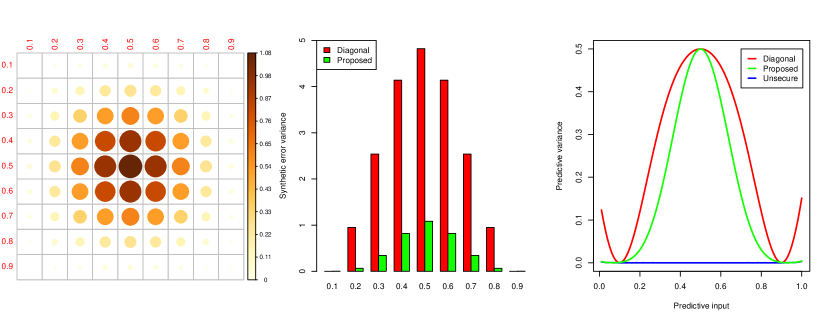
Figure 1: Numerical results for Example 1. Left: Covariance matrix of the synthetic noise of the proposed method. Middle: Comparison between the synthetic noise variances of the method using independent errors (referred to as the diagonal method) and the proposed method, in order to reach the same privacy level. Right: Comparison of the predictive variance of the diagonal method, the proposed method, and the unsecured method (i.e., the ordinary GP regression).

It is worth noting that the proposed method differs from most existing data obfuscation schemes, where the synthetic error components are assumed as independent. To build privacy-aware GPs, however, using correlated error is arguably more appropriate. For comparison, we consider the problem of adding synthetic Gaussian noise whose covariance matrix is diagonal. This is simply adding one additional constraint to (7) to require that ${\Sigma}$ is a diagonal matrix, which also leads to an SDP. Unlike (7), this SDP does not admit an explicit solution but can be pursued using an existing interior point method. As shown in the middle plot of Figure 1, if we enforce the diagonal covariance matrix condition, the required variances to ensure the same privacy level are significantly inflated. The right plot of Figure 1 shows the predictive variances of three methods (uncorrelated synthetic noise, the proposed method, and the ordinary GP regression) with a known covariance structure. It is shown that the resulting predictive variance of the diagonal method is much larger than the proposed method, especially for $x$ near 0 or 1. This is undesirable because we only need to protect the output privacy at $x=0.5$, and adding independent noise creates an unwanted compromise in the GP model’s predictive accuracy. The blue curve in the right plot of Figure 1 is the predictive variance of the ordinary GP regression. Its predictive variance is small, but it cannot fulfill the privacy requirement, that is, the predictive variance at $x=0.5$ should be no less than $0.5$.

4.2 Multiple sensitive inputs

Now suppose that we have multiple sensitive inputs $s_{1},\ldots,s_{\gamma}$. In analogous to the method in Section 4.1, we introduce the corresponding privacy tolerances $\xi_{1},\ldots,\xi_{\gamma}$ and consider the SDP problem

$$\begin{split}&\min_{{\Sigma}}\operatorname{Tr}({\Sigma})\\ \text{subject to: }&{\Sigma}+{K}_{X,X}+{V}-(K_{s_{i},s_{i}}-\xi_{i})^{-1}K_{X,s_{i}}K_{s_{i},X}\geq 0,\text{ for }i=1,\ldots,\gamma\\ &{\Sigma}\geq 0,\end{split}$$ (10)

where we require $\xi_{i}<K_{s_{i},s_{i}}$ similar to (7). Unlike (7), (10) does not admit an explicit solution. We can solve (10) by a convex optimization algorithm such as the interior point method. We call a solution to (10) a weakly privacy-aware solution.

Next we introduce a stronger constraint than that in (10), leading to a strongly privacy-aware solution. The idea is to consider not only the private features $f(s_{1}),\ldots,f(s_{\gamma})$ themselves, but also their linear combinations. Specifically, we enforce the condition $\text{Var}[\sum_{i=1}^{\gamma}\beta_{i}f(s_{i})|W]\geq\beta^{T}\Xi\beta$ for a prespecified PSD matrix $\Xi$ and any $\beta=(\beta_{1},\ldots,\beta_{\gamma})^{T}\in\mathbb{R}^{\gamma}$. Through the Schur complement argument analogous to (7), we arrive at the following SDP problem

$$\begin{split}&\min_{{\Sigma}}\operatorname{Tr}({\Sigma})\\ \text{subject to: }&{\Sigma}+{K}_{X,X}+V-K_{X,S}(K_{S,S}-{\Xi})^{-1}K_{S,X}\geq 0\\ &{\Sigma}\geq 0,\end{split}$$ (11)

with $S=(s_{1},\ldots,s_{\gamma})$. Here we also require that $K_{S,S}-\Xi>0$, which is needed by the validity of the Schur complement argument. By Theorem 1, (11) admits a unique optimizer with explicit expression $(K_{X,S}(K_{S,S}-{\Xi})^{-1}K_{S,X}-{K}_{X,X}-V)^{+}$. The relation between weakly and strongly privacy-aware solutions is characterized by Theorem 2.

Theorem 2.

Let $\Sigma_{weak}$ and $\Sigma_{strong}$ be optimizers of (10) and (11), respectively. Suppose $\xi_{i}=(\Xi)_{ii}$ for each $i$. Then

1. $\operatorname{Tr}(\Sigma_{weak})\leq\operatorname{Tr}(\Sigma_{strong})$;

2. There exists a specific choice of $\Xi$ such that $\Sigma_{weak}=\Sigma_{strong}$.

Example 2.

In this example, we compare the weakly and strongly privacy-aware solutions. Consider the same GP and input points as Example 1 with sensitive inputs $0.4$ and $0.6$. For the weakly privacy-aware case, suppose $\xi_{1}=\xi_{2}=0.5$. For the strongly privacy-aware case, we introduce a parameter $c$ and use $\Xi=\begin{pmatrix}0.5&c\\ c&0.5\end{pmatrix}$. Because $K_{S,S}=\begin{pmatrix}1&e^{-0.4}\\ e^{-0.4}&1\end{pmatrix}$, and we have to fulfill the requirements $\Xi\geq 0$ and $K_{S,S}-\Xi>0$, $c$ has to lie in the interval $(e^{-0.4}-0.5,0.5]\approx(0.17,0.5]$.

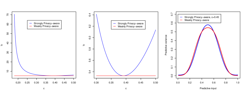
Figure 2: Left and middle: trace of the optimal noise matrix versus $c$, Example 2. Right: predictive variance of the weakly privacy-aware method and the strongly privacy-aware method with $c=0.45$.

The left and middle plots of Figure 2 show the numerical results of the traces of the synthetic noise matrices under strongly and weakly privacy-aware conditions. The left plot gives the original range of $c$; the middle plot zooms into $[0.3,0.5]$. It can be seen that there is no significant difference between the traces of the noise matrices from strongly and weakly privacy-aware conditions for a reasonably wide range of $c$. It is also suggested that the best choice of $\Xi$ should incorporate positive correlations between sensitive inputs, but the correlation should not be too strong. The right plot shows the predictive variance of the strongly privacy-aware GP regression with $c=0.45$, and that of the weakly privacy-aware GP regression. It can be seen that they are not much different. Both methods ensure that the predictive variances at $x=0.4,0.6$ are $0.5$.

It is also worth noting that the predictive variance of the strongly privacy-aware method in Figure 2 is not always larger than that of the weakly privacy-aware method. This implies that $\Sigma_{strong}-\Sigma_{weak}$ is not a PSD matrix, although we have $\operatorname{Tr}(\Sigma_{weak})\leq\operatorname{Tr}(\Sigma_{strong})$ from Theorem 2.

4.3 Kernel-based approach

To define the strongly privacy-aware solution, we need to specify the $\gamma\times\gamma$ PSD matrix $\Xi$ satisfying the constraint $K_{S,S}-\Xi>0$. A general approach is to use a positive semi-definite kernel function $H$ to define $\Xi$, i.e., let $\Xi=H_{S,S}$. In this situation, if we can ensure that $K-H$ is positive definite, we have $K_{S,S}-H_{S,S}>0$ for any $S$. An easy scenario to work with stationary kernels, which are commonly used in GP regression. Suppose both $K$ and $H$ are stationary, i.e., there exist $R_{K},R_{H}:\mathbb{R}^{d}\rightarrow\mathbb{R}$, such that $K(x,y)=R_{K}(x-y),H(x,y)=R_{H}(x-y)$. We further assume that $R_{K}$ and $R_{H}$ are continuous and integrable on $\mathbb{R}^{d}$, which is true for all commonly used stationary kernels. This ensures that $R_{K}$ and $R_{H}$ have real-valued Fourier transforms, denoted as $\tilde{R}_{K}$ and $\tilde{R}_{H}$, respectively. Bochner’s Theorem (Wendland, 2004) asserts that $\tilde{R}_{K}$ and $\tilde{R}_{H}$ must be non-negative, and on the other hand, for each even non-negative even function on $\mathbb{R}^{d}$, its inverse Fourier transform is a positive semi-definite kernel. Proposition 1 gives a sufficient condition to ensure that $R_{K}-R_{H}$ is positive definite.

Proposition 1 (Wendland (2004), Corollary 6.9).

If $\tilde{R}_{K}-\tilde{R}_{H}$ is continuous, non-negative, and is not identical to zero on $\mathbb{R}^{d}$, then $R_{K}-R_{H}$ is positive definite.

Proposition 1 inspires a general method of finding a valid $\Xi$. First find an even continuous function $\tilde{R}_{H}$ satisfying $0\leq\tilde{R}_{H}(\omega)\leq\tilde{R}_{K}(\omega)$ for all $\omega\in\mathbb{R}^{d}$ with $\tilde{R}_{H}(\omega)<\tilde{R}_{K}(\omega)$ for at least one specific $\omega$. Then use the inverse Fourier transform to find the kernel $R_{H}$, and set the $(i,j)$-th entry of $\Xi$ as $R_{H}(s_{i}-s_{j})$.

Example 3.

Suppose $K(x,y)=\exp\{-\theta_{0}\|x-y\|^{2}\}$ and $H(x,y)=c\exp\{-\theta\|x-y\|^{2}\}$, where $x,y\in\mathbb{R}^{d}$, $\theta_{0}>0$ is fix, and $c,\theta\geq 0$ are parameters. Direct calculations show $\tilde{R}_{K}(\omega)=(2\theta_{0})^{-d/2}\exp\{-\|\omega\|^{2}/(4\theta_{0})\}$ and $\tilde{R}_{H}(\omega)=c(2\theta)^{-d/2}\exp\{-\|\omega\|^{2}/(4\theta)\}$. Then $\tilde{R}_{K}(\omega)/\tilde{R}_{H}(\omega)=c^{-1}(\theta/\theta_{0})^{d/2}\exp\{\frac{(\theta_{0}-\theta)\|\omega\|^{2}}{4\theta}\}\geq 1$ for all $\omega\in\mathbb{R}^{d}$ if and only if $0\leq c\leq 1$ and $c^{2/d}\theta_{0}\leq\theta\leq\theta_{0}$. To ensure that $K-H$ is positive definite, we should exclude the case $c=1$. Thus the final range of $(c,\theta)$ is $\{0\leq c<1,c^{2/d}\theta_{0}\leq\theta\leq\theta_{0}\}$. A related numerical example is presented in the Supplementary Materials.

4.4 Infinite sensitive inputs

In practice, the number of sensitive inputs can be infinite. A typical example is that the user wants to protect the output values of $f$ over an open subregion of $\mathbb{R}^{d}$. We will show that the kernel-based strongly privacy-aware solutions in Section 4.3 allows for studying such a problem. Recall that the optimal covariance matrix is

$$\Sigma_{opt}(S):=(K_{X,S}(K_{S,S}-{H_{S,S}})^{-1}K_{S,X}-{K}_{X,X}-V)^{+}.$$ (12)

The goal of this section is to extend the definite of $\Sigma_{opt}(S)$ to a general set $S\subset\mathbb{R}^{d}$.

Our development relies on the theory of reproducing kernel Hilbert spaces (RKHSs) (Aronszajn, 1950; Wendland, 2004; Paulsen and Raghupathi, 2016). This work concerns only RKHSs whose reproducing kernels are positive definite. The definition of these function spaces is detailed in the Supplementary Materials. Denote the RKHS on $\Omega$ with reproducing kernel $\Phi$ as $\mathcal{N}_{\Phi}(\Omega)$, and the norm and inner product by $\|\cdot\|_{\mathcal{N}_{\Phi}(\Omega)}$ and $\langle\cdot,\cdot\rangle_{\mathcal{N}_{\Phi}(\Omega)}$, respectively. While more details of the RKHS theory are presented in the Supplementary Materials, here we need the identity $K_{x_{i},S}(K_{S,S}-{H_{S,S}})^{-1}K_{S,x_{j}}=\langle K(\cdot,x_{i}),K(\cdot,x_{j})\rangle_{\mathcal{N}_{K-H}(S)}$, which leads to the following representation of (12):

$$\Sigma_{opt}(S)=\left(G(S)-{K}_{X,X}-V\right)^{+},$$ (13)

where $G(S)$ denotes the matrix whose $(i,j)$-th entry is $\langle K(\cdot,x_{i}),K(\cdot,x_{j})\rangle_{\mathcal{N}_{K-H}(S)}$. Equation (13) suggests a natural extension of (12) as $S$ can be an arbitrary non-empty subset of $\mathbb{R}^{d}$. The following Theorem 3 implies that $\Sigma_{opt}(S)$ lies in the feasible region of (12) under any finite subset of $S$.

Theorem 3.

Suppose $K-H$ is continuous and positive definite, and $K(\cdot,x_{i})\in\mathcal{N}_{K-H}(S)$ for each $i=1,\ldots,n$. The following statements are true.

1. For each non-empty $S^{\prime}\subset S$, we have $K(\cdot,x_{i})\in\mathcal{N}_{K-H}(S^{\prime})$ for each $i=1,\ldots,n$, and $G(S)-G(S^{\prime})\geq 0$.

2. If a positive definite matrix $P$ satisfies $P-G(S_{0})\geq 0$ for each finite subset $S_{0}\subset S$, then $P-G(S)\geq 0$.

Theorem 3 also implies that if $G(\mathbb{R}^{d})$ exists, then $G(S)$ exists for each $S\subset\mathbb{R}^{d}$. Thus it is of interest to verify whether $K(\cdot,x_{i})\in\mathcal{N}_{K-H}(\mathbb{R}^{d})$. Besides the trivial case $H=\alpha K$ for $0<\alpha<1$, it is most convenient to work with stationary kernels. Let $K(x,y)=R_{K}(x-y)$ and $H(x,y)=R_{H}(x-y)$, and $R_{K}$ and $R_{H}$ are continuous and integrable on $\mathbb{R}^{d}$ so that they admit real-valued Fourier transforms $\tilde{R}_{K}$ and $\tilde{R}_{H}$, respectively. Proposition 2 is a direct consequence of Theorem 10.12 of Wendland (2004).

Proposition 2.

Suppose $\tilde{R}_{K}$ and $\tilde{R}_{H}$ are continuous on $\mathbb{R}^{d}$, satisfying $\tilde{R}_{K}(\omega)\geq\tilde{R}_{H}(\omega)\geq 0$ for each $\omega\in\mathbb{R}^{d}$. Then for any $x\in\mathbb{R}^{d}$, $K(\cdot,x)\in\mathcal{N}_{K-H}(\mathbb{R}^{d})$ if and only if $\int_{\mathbb{R}^{d}}\frac{\tilde{R}_{K}^{2}(\omega)}{\tilde{R}_{K}(\omega)-\tilde{R}_{H}(\omega)}d\omega<\infty$. In addition, for any $x,x^{\prime}\in\mathbb{R}^{d}$,

$$\langle K(\cdot,x),K(\cdot,x^{\prime})\rangle_{\mathcal{N}_{K-H}(\mathbb{R}^{d})}=(2\pi)^{-d/2}\int_{\mathbb{R}^{d}}\frac{\cos(\omega^{T}(x-x^{\prime}))\tilde{R}_{K}^{2}(\omega)}{\tilde{R}_{K}(\omega)-\tilde{R}_{H}(\omega)}d\omega.$$

The covariance matrix $(G(\mathbb{R}^{d})-K_{X,X}-V)^{+}$ ensures privacy for all input points. Thus we call it the uniformly privacy-aware solution.

The next question is how to compute $G(S)$ numerically when $S$ is an infinite set. Theorem 4 shows that, if $S$ is an infinite compact set, $G(S)$ can be well approximated by $G(S_{0})$ if $S_{0}$ is a sufficiently dense finite subset of $S_{0}$.

Theorem 4.

Suppose $K-H$ is continuous and positive definite. Let $S_{n}$ be a sequence of finite subsets of $\mathcal{X}$. Suppose $S_{n}$ has a limit and denote the closure of $\lim_{n\rightarrow\infty}S_{n}$ as $\bar{S}$. Suppose $\bar{S}$ is a compact set. If $K(\cdot,x_{i})\in\mathcal{N}_{K-H}(\bar{S})$ for each $i$, $G(S_{n})\rightarrow G(\bar{S})$, and therefore, $\Sigma_{opt}(S_{n})\rightarrow\Sigma_{opt}(\bar{S})$, as $n\rightarrow\infty$.

Theorem 4 provides a general consistency result, but there is no rate of convergence. In the Supplementary Materials, we link this convergence rate to the approximation theory of radial basis functions in the RKHS (Wendland, 2004; Rieger, 2008; Rieger and Zwicknagl, 2010; Rieger and Wendland, 2017) under the condition $H=\alpha K$ for $0<\alpha<1$. It is worth noting that when $H=\alpha K$ for $0<\alpha<1$ and $S\supset\{x_{1},\ldots,x_{n}\}$, $G(S)=G(\mathbb{R}^{d})=(1-\alpha)^{-1}K_{X,X}$, i.e., the solution ensuring privacy at all input locations equals the uniformly privacy-aware solution.

5 Application to Tracking of Space Objects

Now we use the data from a mathematical model that describes the trajectories of satellites to illustrate the proposed methodology.

Space situational awareness (SSA) is crucial for tracking and predicting the location of objects in Earth’s orbit to avoid collisions, especially as space becomes more congested. Nations and commercial operators are working together to increase satellite operation safety by exchanging information about space objects, despite privacy and security concerns. Restrictive policies for sharing data from military-owned sensors have led to a lack of confidence in the provided data, and national security concerns are heightened due to anti-satellite weapons and other counter-space capabilities. Commercial operators also worry about competitors accessing sensitive information.

To address these challenges, the SSA mission requires rigorous inclusion of uncertainty in the space surveillance network. High-fidelity models are developed to predict space objects’ locations, but these models contain proprietary features that cannot be shared. As a result, data-driven surrogate models must be created from simulation data and observations for different stakeholders to use in SSA tasks. The challenge lies in constructing accurate surrogate models that enable proper SSA functionality while protecting military and commercial features.

Now we consider a simple satellite dynamics model presented in the Supplementary Materials. Here we consider the input-output between the time (normalized using $T_{orb}$, the time for one orbit) and the length (normalized using $R_{e}$, the radius of Earth).

Figure 3: Satellite dynamics example.

The location of the satellite is described in a polar coordinate system. Figure 3 shows the true curve of the satellite length, in which the presumed private segments in the state trajectories are shown in red. We do not want the privacy-aware GP model to provide accurate predictions in these segments. To build a surrogate model, we sample 61 points from the curve with evenly spaced input values from the input domain $[0,3]$. We use the GP model with correlation function $\exp\{-200x^{2}\}$ and use the maximum likelihood method to estimate the constant mean and the variance of the GP. The obfuscated data are shown by the blue dots, and the $\pm 2\sigma$ confidence limits are shown by the green curves. We use the kernel-based approach and consider two choices of $H$: $H=0.1K$ and $H=0.5K$. It can be seen that only the private segment is affected by data obfuscation. With $H=0.5K$, the predictive curve is corrupted as the confidence band becomes much larger, and with $H=0.1K$, the private trajectory is completely hidden so the users cannot see any details in this segment.

Privacy-aware GP regression models are built for other trajectories (the angle and the velocities). These results, together with further discussions, are presented in the Supplementary Materials.

6 Discussion

In this work, we establish the first theoretical and methodological framework for privacy-aware GP regression. Like any machine learning method that addresses privacy concerns, the proposed method safeguards privacy at the cost of predictive accuracy. While the privacy levels are fully in control, the proposed method does not guarantee fit-for-use predictive outputs. Users should validate the utility of the resulting privacy-aware GP models by checking whether the predictive confidence bars are acceptable. Failure to do so may result in a negative societal impact of presenting unsatisfactory and misleading predictions.

Whether the weakly privacy-aware problem (10) has a unique solution is an unaddressed theoretical question and requires further investigation. Similar to the usual GP regression, finding the synthetic covariance matrix faces computational challenges when the sample size is large. Some recent techniques in scalable GP regression (Quinonero-Candela and Rasmussen, 2005; Rahimi and Recht, 2007; Titsias, 2009; Hartikainen and Särkkä, 2010; Hensman et al., 2013; Plumlee, 2014; Gramacy and Apley, 2015; Wilson and Nickisch, 2015; Grigorievskiy et al., 2017; Nickisch et al., 2018; Wang et al., 2019; Katzfuss and Guinness, 2021; Ding et al., 2023; Chen et al., 2022; Yadav et al., 2022) can be adapted to compute certain components in the proposed method, such as $G(S)$, efficiently. Finding weakly privacy-aware solutions relies on SDP, which is, albeit polynomial-time solvable in theory, not scalable under most commonly used SDP software packages, e.g. CVX (Grant and Boyd, 2014) or CVXPY (Diamond and Boyd, 2016). More efficient algorithms should be developed if one prefers these solutions. The strongly and kernel-based privacy-aware solutions, however, only rely on finding the positive definite part of a symmetric matrix, which can be done must faster. In particular, recent developments in fast computation of the square roots of PSD matrices (Pleiss et al., 2020; Hale et al., 2008) enable an $O(n^{2})$ time algorithm in view of the identity $\mathbf{A}^{+}=(\mathbf{A}+\sqrt{\mathbf{A}^{2}})/2$.

References

- Aronszajn (1950) Nachman Aronszajn. Theory of reproducing kernels. Transactions of the American Mathematical Society, 68(3):337–404, 1950.
- Chen et al. (2022) Haoyuan Chen, Liang Ding, and Rui Tuo. Kernel packet: An exact and scalable algorithm for Gaussian process regression with Matérn correlations. Journal of Machine Learning Research, 23(127):1–32, 2022.
- Cressie (1993) Noel Cressie. Statistics for Spatial Data. Wiley-Interscience, 2 edition, 1993.
- Diamond and Boyd (2016) Steven Diamond and Stephen Boyd. CVXPY: A Python-embedded modeling language for convex optimization. The Journal of Machine Learning Research, 17(1):2909–2913, 2016.
- Ding et al. (2023) Liang Ding, Rui Tuo, and Shahin Shahrampour. A sparse expansion for deep Gaussian processes. IISE Transactions, Accepted, 2023.
- Ghosh and Kleinberg (2016) Arpita Ghosh and Robert Kleinberg. Inferential privacy guarantees for differentially private mechanisms. arXiv preprint arXiv:1603.01508, 2016.
- Gramacy (2020) Robert B Gramacy. Surrogates: Gaussian Process Modeling, Design, and Optimization for the Applied Sciences. Chapman and Hall/CRC, 2020.
- Gramacy and Apley (2015) Robert B Gramacy and Daniel W Apley. Local Gaussian process approximation for large computer experiments. Journal of Computational and Graphical Statistics, 24(2):561–578, 2015.
- Grant and Boyd (2014) Michael Grant and Stephen Boyd. CVX: Matlab software for disciplined convex programming, version 2.1, 2014.
- Grigorievskiy et al. (2017) Alexander Grigorievskiy, Neil Lawrence, and Simo Särkkä. Parallelizable sparse inverse formulation Gaussian processes (SpInGP). In 2017 IEEE 27th International Workshop on Machine Learning for Signal Processing (MLSP), pages 1–6. IEEE, 2017.
- Hale et al. (2008) Nicholas Hale, Nicholas J Higham, and Lloyd N Trefethen. Computing ,, and related matrix functions by contour integrals. SIAM Journal on Numerical Analysis, 46(5):2505–2523, 2008.
- Hartikainen and Särkkä (2010) Jouni Hartikainen and Simo Särkkä. Kalman filtering and smoothing solutions to temporal Gaussian process regression models. In 2010 IEEE International Workshop on Machine Learning for Signal Processing, pages 379–384. IEEE, 2010.
- Hensman et al. (2013) James Hensman, Nicolo Fusi, and Neil D Lawrence. Gaussian processes for big data. arXiv preprint arXiv:1309.6835, 2013.
- Katzfuss and Guinness (2021) Matthias Katzfuss and Joseph Guinness. A general framework for Vecchia approximations of Gaussian processes. Statistical Science, 36(1):124–141, 2021.
- Nickisch et al. (2018) Hannes Nickisch, Arno Solin, and Alexander Grigorevskiy. State space Gaussian processes with non-Gaussian likelihood. In International Conference on Machine Learning, pages 3789–3798. PMLR, 2018.
- Paulsen and Raghupathi (2016) Vern I Paulsen and Mrinal Raghupathi. An Introduction to the Theory of Reproducing Kernel Hilbert Spaces, volume 152. Cambridge university press, 2016.
- Pleiss et al. (2020) Geoff Pleiss, Martin Jankowiak, David Eriksson, Anil Damle, and Jacob Gardner. Fast matrix square roots with applications to Gaussian processes and Bayesian optimization. Advances in Neural Information Processing Systems, 33:22268–22281, 2020.
- Plumlee (2014) Matthew Plumlee. Fast prediction of deterministic functions using sparse grid experimental designs. Journal of the American Statistical Association, 109(508):1581–1591, 2014.
- Press et al. (2007) William H Press, Saul A Teukolsky, William T Vetterling, and Brian P Flannery. Numerical Recipes: The Art of Scientific Computing (3rd Edition). Cambridge university press, 2007.
- Quinonero-Candela and Rasmussen (2005) Joaquin Quinonero-Candela and Carl Edward Rasmussen. A unifying view of sparse approximate Gaussian process regression. The Journal of Machine Learning Research, 6:1939–1959, 2005.
- Rahimi and Recht (2007) Ali Rahimi and Benjamin Recht. Random features for large-scale kernel machines. Advances in Neural Information Processing Systems, 20, 2007.
- Rasmussen and Williams (2006) C. E. Rasmussen and K. I. Williams. Gaussian Processes for Machine Learning. MIT Press, 2006.
- Rieger (2008) Christian Rieger. Sampling inequalities and applications. PhD thesis, Citeseer, 2008.
- Rieger and Wendland (2017) Christian Rieger and Holger Wendland. Sampling inequalities for sparse grids. Numerische Mathematik, 136(2):439–466, 2017.
- Rieger and Zwicknagl (2010) Christian Rieger and Barbara Zwicknagl. Sampling inequalities for infinitely smooth functions, with applications to interpolation and machine learning. Advances in Computational Mathematics, 32:103–129, 2010.
- Santner et al. (2003) Thomas J Santner, Brian J Williams, and William I Notz. The Design and Analysis of Computer Experiments. Springer, 2003.
- Song and Chaudhuri (2017) Shuang Song and Kamalika Chaudhuri. Composition properties of inferential privacy for time-series data. In 2017 55th Annual Allerton Conference on Communication, Control, and Computing (Allerton), pages 814–821. IEEE, 2017.
- Stein (1999) Michael L Stein. Interpolation of Spatial Data: Some Theory for Kriging. Spring, 1999.
- Sun and Tay (2017) Meng Sun and Wee Peng Tay. Inference and data privacy in IoT networks. In 2017 IEEE 18th International Workshop on Signal Processing Advances in Wireless Communications (SPAWC), pages 1–5. IEEE, 2017.
- Titsias (2009) Michalis Titsias. Variational learning of inducing variables in sparse Gaussian processes. In Artificial Intelligence and Statistics, pages 567–574. PMLR, 2009.
- Wang et al. (2019) Ke Wang, Geoff Pleiss, Jacob Gardner, Stephen Tyree, Kilian Q Weinberger, and Andrew Gordon Wilson. Exact gaussian processes on a million data points. Advances in Neural Information Processing Systems, 32, 2019.
- Wendland (2004) Holger Wendland. Scattered Data Approximation, volume 17. Cambridge University Press, 2004.
- Wilson and Nickisch (2015) Andrew Wilson and Hannes Nickisch. Kernel interpolation for scalable structured Gaussian processes (KISS-GP). In International Conference on Machine Learning, pages 1775–1784. PMLR, 2015.
- Yadav et al. (2022) Mohit Yadav, Daniel R Sheldon, and Cameron Musco. Kernel interpolation with sparse grids. Advances in Neural Information Processing Systems, 35:22883–22894, 2022.
- Zhang (2006) Fuzhen Zhang. The Schur Complement and Its Applications, volume 4. Springer Science & Business Media, 2006.