Vector-Valued Variation Spaces and Width Bounds for DNNs:
Insights on Weight Decay Regularization

Abstract

Deep neural networks (DNNs) trained to minimize a loss term plus the sum of squared weights via gradient descent corresponds to the common approach of training with weight decay. This paper provides new insights into this common learning framework. We characterize the kinds of functions learned by training with weight decay for multi-output (vector-valued) ReLU neural networks. This extends previous characterizations that were limited to single-output (scalar-valued) networks. This characterization requires the definition of a new class of neural function spaces that we call vector-valued variation (VV) spaces. We prove that neural networks (NNs) are optimal solutions to learning problems posed over VV spaces via a novel representer theorem. This new representer theorem shows that solutions to these learning problems exist as vector-valued neural networks with widths bounded in terms of the number of training data. Next, via a novel connection to the multi-task lasso problem, we derive new and tighter bounds on the widths of homogeneous layers in DNNs. The bounds are determined by the effective dimensions of the training data embeddings in/out of the layers. This result sheds new light on the architectural requirements for DNNs. Finally, the connection to the multi-task lasso problem suggests a new approach to compressing pre-trained networks.

Keywords: deep neural networks, regularization, sparsity, variation spaces, weight decay, multi-task lasso

1 Introduction

Training a deep neural network (DNN) with weight decay and gradient descent corresponds to regularizing with the sum of squared weights. This is a simple yet effective form of regularization that is widely used in practice with many benefits (Bartlett, 1996; Krogh and Hertz, 1991; Bos and Chug, 1996; Zhang et al., 2021; Power et al., 2021; Zhai et al., 2019; Kolesnikov et al., 2020). This paper studies the effect of weight decay on NNs and/or network layers consisting of homogeneous units such as the Rectified Linear Unit (ReLU).

We study DNNs $f_{{\bm{\theta}}}$ that solve the weight decay objective

$$\min_{{\bm{\theta}}}\sum_{i=1}^{N}\mathcal{L}({\bm{y}}_{i},f_{{\bm{\theta}}}({\bm{x}}_{i}))+\frac{\lambda}{2}\|{\bm{\theta}}\|^{2}_{2}.$$ (1)

where ${\bm{\theta}}$ is a vector containing all of the DNN weights and $\mathcal{L}(\mkern 1.0mu\cdot\mkern 1.0mu,\mkern 1.0mu\cdot\mkern 1.0mu)$ is a lower semicontinuous loss function.

Often, DNNs contain many homogeneous activation functions, such as the ReLU. An activation function $\sigma(z)$ is homogeneous (of degree $1$) if $\sigma(cz)=c\sigma(z)$ for any $c>0$. A key observation both in theory (Grandvalet, 1998; Neyshabur et al., 2015; Parhi and Nowak, 2020; Ongie et al., 2020; Jacot, 2023) and practice (Kunin et al., 2021) is that for any DNN that solves (1) the 2-norms of the input and output weights of each homogeneous unit are balanced. This phenomenon is referred to as the neural balance theorem (NBT) (Yang et al., 2022, Theorem 1), which is summarized below.

Theorem 1 (Neural Balance Theorem (NBT))

Let $f_{\bm{\theta}}$ be a DNN of any architecture parameterized by ${\bm{\theta}}\in\Theta$ which solves Eq. 1. Then, the weights satisfy the following balance constraint: if ${\bm{w}}$ and ${\bm{v}}$ denote the input and output weights of any homogeneous unit in the DNN, then $\lVert{\bm{w}}\rVert_{2}=\lVert{\bm{v}}\rVert_{2}$.

While the NBT is a simple observation, it allows for an alternative perspective on the weight decay regularizer. Concretely, consider the shallow vector-valued NN mapping $\mathbb{R}^{d}\to\mathbb{R}^{D}$ with a homogeneous activation function $\sigma:\mathbb{R}\to\mathbb{R}$ of the form

$$f_{\bm{\theta}}({\bm{x}})=\sum_{k=1}^{K}{\bm{v}}_{k}\sigma\left({\bm{w}}_{k}^{T}\begin{bmatrix}{\bm{x}}\\ 1\end{bmatrix}\right),\quad{\bm{x}}\in\mathbb{R}^{d},\>{\bm{\theta}}=({\bm{v}}_{k},{\bm{w}}_{k})_{k=1}^{K},$$

where ${\bm{v}}_{k}\in\mathbb{R}^{D}$ and ${\bm{w}}_{k}\in\mathbb{R}^{d+1}$. A consequence of the NBT is that any solution to the NN training problem with weight decay

$$\min_{{\bm{\theta}}}\sum_{i=1}^{N}{\mathcal{L}}({\bm{y}}_{i},f_{{\bm{\theta}}}({\bm{x}}_{i}))+\frac{\lambda}{2}\sum_{k=1}^{K}\|{\bm{w}}_{k}\|_{2}^{2}+\|{\bm{v}}_{k}\|_{2}^{2}$$ (2)

is also a solution to

$$\min_{{\bm{\theta}}}\sum_{i=1}^{N}{\mathcal{L}}({\bm{y}}_{i},f_{{\bm{\theta}}}({\bm{x}}_{i}))+\lambda\sum_{k=1}^{K}\|{\bm{w}}_{k}\|_{2}\|{\bm{v}}_{k}\|_{2}.$$ (3)

Moreover after a rebalancing step of the weights, any solution to Eq. 3 is also a solution to Eq. 2. Thus, the problems in Eqs. 2 and 3 are equivalent. We refer the reader to Yang et al. (2022) or the recent survey of Parhi and Nowak (2023b) for more details about this equivalence and its effect on training DNNs. This observation brings about many remarkable implications. In this paper we exploit this connection and bring several new results.

A novel characterization of the kinds of functions learned by NNs trained with weight decay.

We propose a new class of neural function spaces called vector-valued variation (VV) spaces. These infinite-dimensional spaces reduce to standard variation spaces (Kurková and Sanguineti, 2001; Mhaskar, 2004; Bach, 2017) for NNs with single outputs, but more generally VV spaces are the natural spaces associated with multi-output (vector-valued) NNs trained with weight decay; e.g., NNs in multiclass learning problems. We prove a representer theorem which states that finite-width NNs are optimal solutions to data-fitting problems in VV spaces. Analyzing the VV spaces reveals that weight decay favors solutions in which different outputs share neurons, as opposed to networks that use disjoint subsets of neurons for each output. The representer theorem also provides an upper bound on the required width of each layer, depending on the number of training examples and the output dimension of the network. Furthermore, we prove that the VV spaces are “immune” to the curse of dimensionality since they admit dimension-free approximation rates.

Tighter bounds on DNN widths.

We show how the weights that solve Eq. 1 must also be solutions to a constrained convex optimization, posed over each layer in the deep neural network. Through this connection, we derive new and tighter bounds on the necessary widths of deep neural network layers. The bounds are determined by the effective dimensions of the training data embeddings in/out of the layers, which can be significantly smaller than the previously best known bound found in Jacot et al. (2022, Proposition 7). This sheds new light on architectural requirements for neural nets. Moreover, the connection to the convex optimization suggests a new approach to pruning pre-trained networks. The bounds are based on a reduction to the so-called multi-task lasso problem Obozinski et al. (2006, 2010); Argyriou et al. (2008), and our results provide a novel characterization of the sparsity of multi-task lasso solutions, in general.

2 Vector-Valued Variation Spaces and Weight Decay

In this section, we propose a new NN Banach space which we call the vector-valued variation (VV) space. The name refers to the fact that the norm that defines the space is a new type of variation norm (related to the concept of total variation) which generalizes the standard scalar-valued variation spaces and variation norms that have previously been studied (Kurková and Sanguineti, 2001; Mhaskar, 2004; Bach, 2017). We show that shallow, vector-valued NNs with homogeneous (of degree $1$) activation functions (e.g., the ReLU) trained with weight decay are optimal functions in the VV space. To establish this result, we prove a novel representer theorem that shows that finite-width vector-valued NNs are optimal solutions to data-fitting problems in the VV space. This result sheds new light on the kind of regularity that weight decay encourages. While we only focus on activation functions that are homogeneous of degree $1$, it is clear how the results generalize to any positively homogeneous activation function (e.g., powers of the ReLU). The primary technical difficulty that arises when defining the VV spaces boils down to which choice of norm the space should be equipped with. Indeed, as we will see in Section 2.2 there are many choices of equivalent norms, but only one corresponds to weight decay.

2.1 Scalar-Valued Variation Spaces

As a warm-up, before we define the vector-valued variation spaces, we first review the definition of the classical, scalar-valued variation spaces and their connection to training NNs with weight decay. The results stated in this subsection can be found in Bengio et al. (2005); Bach (2017); Parhi and Nowak (2021); Siegel and Xu (2023). The main idea is to consider shallow NNs with possibly continuously many neurons. These NNs are parameterized by a finite (Radon) measure. The scalar-valued variation space is the space of functions mapping $\mathbb{R}^{d}\to\mathbb{R}$

$$\mathcal{V}(\mathbb{R}^{d})\coloneqq\left\{f({\bm{x}})=\int_{\mathbb{S}^{d}}\sigma({\bm{w}}^{T}\overline{{\bm{x}}})\,\mathrm{d}\nu({\bm{w}})\>\colon\>{\bm{x}}\in\mathbb{R}^{d},\nu\in\mathcal{M}(\mathbb{S}^{d})\right\},$$

where $\mathbb{S}^{d}\coloneqq\{{\bm{w}}\in\mathbb{R}^{d+1}\>\colon\>\lVert{\bm{w}}\rVert_{2}=1\}$ is the unit sphere, $\overline{{\bm{x}}}\coloneqq[{\bm{x}}\ 1]^{T}\in\mathbb{R}^{d+1}$ augments ${\bm{x}}$ to account for a bias term, and $\mathcal{M}(\mathbb{S}^{d})$ is the space of finite (Radon) measures. Since each function $f\in\mathcal{V}(\mathbb{R}^{d})$ is parameterized by a measure $\nu\in\mathcal{M}(\mathbb{S}^{d})$, we introduce the notation

$$f_{\nu}({\bm{x}})\coloneqq\int_{\mathbb{S}^{d}}\sigma({\bm{w}}^{T}\overline{{\bm{x}}})\,\mathrm{d}\nu({\bm{w}}),\quad{\bm{x}}\in\mathbb{R}^{d}.$$ (4)

The space $\mathcal{V}(\mathbb{R}^{d})$ is a Banach space when equipped with the norm

$$\lVert f\rVert_{\mathcal{V}(\mathbb{R}^{d})}\coloneqq\inf_{\begin{subarray}{c}\nu\in\mathcal{M}(\mathbb{S}^{d})\\ f=f_{\nu}\end{subarray}}\lVert\nu\rVert_{\mathcal{M}(\mathbb{S}^{d})},$$ (5)

where $\lVert\mkern 1.0mu\cdot\mkern 1.0mu\rVert_{\mathcal{M}(\mathbb{S}^{d})}$ denotes the total variation norm in the sense of measures.

The requirement of the $\inf$ in the definition of the norm arises since the dictionary of neurons $\{{\bm{x}}\mapsto\sigma({\bm{w}}^{T}\overline{{\bm{x}}})\}_{{\bm{w}}\in\mathbb{S}^{d}}$ is highly redundant. Thus, there are many different representations for a given $f\in\mathcal{V}(\mathbb{R}^{d})$. By choosing the representation with the smallest total variation norm, Eq. 5 defines a valid Banach norm on $\mathcal{V}(\mathbb{R}^{d})$. Here, we use the following definition of $\lVert\mkern 1.0mu\cdot\mkern 1.0mu\rVert_{\mathcal{M}(\mathbb{S}^{d})}$

$$\lVert\nu\rVert_{\mathcal{M}(\mathbb{S}^{d})}\coloneqq\sup_{\begin{subarray}{c}\mathbb{S}^{d}=\bigcup_{i=1}^{n}A_{i}\\ n\in\mathbb{N}\end{subarray}}\sum_{i=1}^{n}\lvert\nu(A_{i})\rvert,$$ (6)

where $\sup$ is taken over all partitions of $\mathbb{S}^{d}$ (i.e., $A_{i}\cap A_{j}=\varnothing$ for $i\neq j$). This definition is equal to the more conventional definition based on the Jordan decomposition of a measure or the definition as a dual norm (Diestel and Uhl, 1977; Bredies and Holler, 2020). That is,

$$\lVert\nu\rVert_{\mathcal{M}(\mathbb{S}^{d})}=\nu^{+}(\mathbb{S}^{d})+\nu^{-}(\mathbb{S}^{d})=\sup_{\begin{subarray}{c}g\in C(\mathbb{S}^{d})\\ \lVert g\rVert_{L^{\infty}}=1\end{subarray}}\int_{\mathbb{S}^{d}}g({\bm{u}})\,\mathrm{d}\nu({\bm{u}}),$$

where $\nu=\nu^{+}-\nu^{-}$ is the Jordan decomposition of $\nu$ and $C(\mathbb{S}^{d})$ is the space of continuous functions on $\mathbb{S}^{d}$. We use definition in Eq. 6 as an analogous definition will play an important role in the vector-valued case.

Consider a single neuron $\phi_{v,{\bm{w}}}({\bm{x}})\coloneqq v\sigma({\bm{w}}^{T}\overline{{\bm{x}}})$, ${\bm{x}}\in\mathbb{R}^{d}$, where $v\in\mathbb{R}$ and ${\bm{w}}\in\mathbb{R}^{d+1}$. Since $\sigma$ is homogeneous of degree $1$, we have $\phi_{v,{\bm{w}}}({\bm{x}})=v\lVert{\bm{w}}\rVert_{2}\sigma({\bm{w}}^{T}\overline{{\bm{x}}}/\lVert{\bm{w}}\rVert_{2})$. In this scenario, it is clear that the $\inf$ in Eq. 5 is achieved by the one scaled Dirac measure $v\lVert{\bm{w}}\rVert_{2}\delta_{{\bm{w}}/\lVert{\bm{w}}\rVert_{2}}$. Thus, if we have the shallow NN

$$f_{\bm{\theta}}({\bm{x}})=\sum_{k=1}^{K}v_{k}\sigma({\bm{w}}_{k}^{T}\overline{{\bm{x}}}),\quad{\bm{x}}\in\mathbb{R}^{d},\>{\bm{\theta}}=(v_{k},{\bm{w}}_{k})_{k=1}^{K},$$

where $v_{k}\in\mathbb{R}$ and the input weights ${\bm{w}}_{k}\in\mathbb{R}^{d+1}$ are all unique after normalization, we have that the $\inf$ is achieved by

$$\sum_{k=1}^{K}v_{k}\lVert{\bm{w}}_{k}\rVert_{2}\delta_{{\bm{w}}_{k}/\lVert{\bm{w}}_{k}\rVert_{2}}.$$

Therefore,

$$\lVert f_{\bm{\theta}}\rVert_{\mathcal{V}(\mathbb{R}^{d})} =\left\lVert\sum_{k=1}^{K}v_{k}\lVert{\bm{w}}_{k}\rVert_{2}\delta_{{\bm{w}}_{k}/\lVert{\bm{w}}_{k}\rVert_{2}}\right\rVert_{\mathcal{M}(\mathbb{S}^{d})}$$

$$=\sum_{k=1}^{K}\Big{\lVert}v_{k}\lVert{\bm{w}}_{k}\rVert_{2}\delta_{{\bm{w}}_{k}/\lVert{\bm{w}}_{k}\rVert_{2}}\Big{\rVert}_{\mathcal{M}(\mathbb{S}^{d})}$$

$$=\sum_{k=1}^{K}\lvert v_{k}\rvert\lVert{\bm{w}}_{k}\rVert_{2},$$ (7)

where in the second line we used the fact that the Dirac measures have disjoint support and in the third line we used the property that $\lVert a\delta_{{\bm{u}}}\rVert_{\mathcal{M}(\mathbb{S}^{d})}=\lvert a\rvert$, where $a\in\mathbb{R}$ and ${\bm{u}}\in\mathbb{S}^{d}$. The quantity Eq. 7 is often referred to as the path-norm (Neyshabur et al., 2015). Furthermore, it is well-known that regularizing a NN with the path-norm is equivalent to the weight decay regularizer (cf., Parhi and Nowak, 2021, Theorem 8). Therefore, training a scalar-output shallow NN with weight decay penalizes the variation norm of the network. This connection is even tighter thanks to the following Banach space representer theorem for the variation spaces.

Proposition 2 (Parhi and Nowak (2021))

Let $({\bm{x}}_{1},y_{1}),\ldots,({\bm{x}}_{N},y_{N})\in\mathbb{R}^{d}\times\mathbb{R}$ be a finite dataset. Then, there exists a solution to the variational problem

$$\inf_{f\in\mathcal{V}(\mathbb{R}^{d})}\>\sum_{i=1}^{N}\mathcal{L}(y_{i},f({\bm{x}}_{i}))+\lambda\lVert f\rVert_{\mathcal{V}(\mathbb{R}^{d})},\quad\lambda>0,$$ (8)

where the loss function $\mathcal{L}(\mkern 1.0mu\cdot\mkern 1.0mu,\mkern 1.0mu\cdot\mkern 1.0mu)$ is lower semicontinuous in its second argument, that takes the form

$$f^{\star}({\bm{x}})=\sum_{k=1}^{K_{0}}v_{k}\sigma({\bm{w}}_{k}^{T}\overline{{\bm{x}}}),\quad{\bm{x}}\in\mathbb{R}^{d},$$

where $K_{0}\leq N$. Here, $v_{k}\in\mathbb{R}$ and ${\bm{w}}_{k}\in\mathbb{S}^{d}$.

Remark 3

We note that earlier the works Rosset et al. (2007); Bach (2017) have also considered similar infinite-dimensional variational problems of this form and argue that the solutions admit a finite-parameter representation.

This representer theorem establishes, in particular, that training a sufficiently wide NN (width $K\geq N$) with path-norm regularization Eq. 7 to a global minimizer results in a solution to Eq. 8. By the equivalence of the path-norm regularizer with weight decay, this result says that any solution to the NN training problem

$$\min_{{\bm{\theta}}}\>\sum_{i=1}^{N}\mathcal{L}(y_{i},f({\bm{x}}_{i}))+\frac{\lambda}{2}\sum_{k=1}^{K}\lvert v_{k}\rvert^{2}+\lVert{\bm{w}}_{k}\rVert_{2}^{2},\quad\lambda>0,$$ (9)

is a solution to Eq. 8, so long as $K\geq N$. We refer the reader to Parhi and Nowak (2021, Section 2.3) for more details about this correspondence. Therefore, the regularity (or “smoothness”) of the solutions to Eq. 9 is exactly quantified by the $\mathcal{V}(\mathbb{R}^{d})$-norm. Furthermore, the $\mathcal{V}(\mathbb{R}^{d})$-norm has an analytical description, via the Radon transform (Ongie et al., 2020; Parhi and Nowak, 2021, 2023a). An interesting observation is that the problem in Eq. 8 is convex, while the problem in Eq. 9 is nonconvex. Thus, by lifting the NN training problem to the space of measures, the training problem has been made convex. For this reason, NNs as in Eq. 4 are sometimes called convex neural networks (Bengio et al., 2005; Bach, 2017).

2.2 Vector-Valued Variation Spaces

The tight connections between weight decay and $\mathcal{V}(\mathbb{R}^{d})$ give key insight into the regularity of solutions to neural network training problems. Unfortunately, these results are not straightforward to extend to the vector-valued (or deep) case. In this section we properly define the vector-valued analog of the variation space such that the connection to weight decay remains. While it is clear that the vector-valued variation space is the set of functions

$$\mathcal{V}(\mathbb{R}^{d};\mathbb{R}^{D})\coloneqq\left\{f({\bm{x}})=\int_{\mathbb{S}^{d}}\sigma({\bm{w}}^{T}\overline{{\bm{x}}})\,\mathrm{d}{\bm{\nu}}({\bm{w}})\>\colon\>{\bm{x}}\in\mathbb{R}^{d},{\bm{\nu}}\in\mathcal{M}(\mathbb{S}^{d};\mathbb{R}^{D})\right\},$$

where ${\bm{\nu}}$ is now a vector-valued measure (which takes values in $\mathbb{R}^{D}$ as opposed to $\mathbb{R}$), the primary difficulty arises with which choice of norm to impose on the vector-valued measures ${\bm{\nu}}\in\mathcal{M}(\mathbb{S}^{d};\mathbb{R}^{D})$ such that there remains a correspondence with weight decay. Indeed, $\mathcal{M}(\mathbb{S}^{d};\mathbb{R}^{D})$ can be equipped with many (equivalent) norms that result in different regularizations of the NN parameters. There have been two lines of work constructing vector-valued variation spaces (Parhi and Nowak, 2022; Korolev, 2022). Unfortunately, neither of these approaches result in NN regularization that corresponds to weight decay.

By viewing $\mathcal{M}(\mathbb{S}^{d};\mathbb{R}^{D})$ as the $D$-fold Cartesian product $\bigtimes_{j=1}^{D}\mathcal{M}(\mathbb{S}^{d})$, a naïve choice of norm would be the mixed norm

$$\lVert{\bm{\nu}}\rVert_{\mathcal{M},p}\coloneqq\left(\sum_{j=1}^{D}\lVert\nu_{j}\rVert_{\mathcal{M}(\mathbb{S}^{d})}^{p}\right)^{1/p}=\left(\sum_{j=1}^{D}\left(\sup_{\begin{subarray}{c}\mathbb{S}^{d}=\bigcup_{i=1}^{n}A_{i}\\ n\in\mathbb{N}\end{subarray}}\sum_{i=1}^{n}\lvert\nu_{j}(A_{i})\rvert\right)^{p}\right)^{1/p},$$

with $p\geq 1$ and ${\bm{\nu}}=(\nu_{1},\ldots,\nu_{D})$ where each $\nu_{j}\in\mathcal{M}(\mathbb{S}^{d})$, $j=1,\ldots,D$. A different choice of norm would be

$$\lVert{\bm{\nu}}\rVert_{p,\mathcal{M}}\coloneqq\sup_{\begin{subarray}{c}\mathbb{S}^{d}=\bigcup_{i=1}^{n}A_{i}\\ n\in\mathbb{N}\end{subarray}}\sum_{i=1}^{n}\lVert{\bm{\nu}}(A_{i})\rVert_{p}=\sup_{\begin{subarray}{c}\mathbb{S}^{d}=\bigcup_{i=1}^{n}A_{i}\\ n\in\mathbb{N}\end{subarray}}\sum_{i=1}^{n}\left(\sum_{j=1}^{D}\lvert\nu_{j}(A_{i})\rvert^{p}\right)^{1/p},$$

with $p\geq 1$. The choice of norm in the above display is the usual definition for the total variation norm of a vector-valued measure. Furthermore, it is well-known that $(\mathcal{M}(\mathbb{S}^{d};\mathbb{R}^{D}),\lVert\mkern 1.0mu\cdot\mkern 1.0mu\rVert_{p,\mathcal{M}})$ is a Banach space. We refer the reader to the monograph of Diestel and Uhl (1977) for a full treatment of vector-valued (and more generally, Banach-valued) measures and the accompanying results.

In essence, the key difference between $\lVert\mkern 1.0mu\cdot\mkern 1.0mu\rVert_{\mathcal{M},p}$ and $\lVert\mkern 1.0mu\cdot\mkern 1.0mu\rVert_{p,\mathcal{M}}$ is the order of the $p$-norm and $\mathcal{M}$-norm. In typical scenarios in which a Banach space is defined by a mixed norm, changing the order of the norms results in different a Banach space. In the present scenario, since $\mathbb{R}^{D}$ is finite-dimensional, it turns out that $\lVert\mkern 1.0mu\cdot\mkern 1.0mu\rVert_{\mathcal{M},p}$ and $\lVert\mkern 1.0mu\cdot\mkern 1.0mu\rVert_{q,\mathcal{M}}$ are equivalent norms for any $p,q\geq 1$. This is summarized in the following lemma.

Lemma 4

The norms $\lVert\mkern 1.0mu\cdot\mkern 1.0mu\rVert_{p,\mathcal{M}}$, $p\geq 1$, and $\lVert\mkern 1.0mu\cdot\mkern 1.0mu\rVert_{\mathcal{M},q}$, $q\geq 1$, are all equivalent Banach norms for $\mathcal{M}(\mathbb{S}^{d};\mathbb{R}^{D})$.

While this result seems obvious, we could not find a proof in the literature. We provide a proof of Lemma 4 in Appendix A. We also note that the reader can quickly verify that when $D=1$, all norms in Lemma 4 are equal.

Thus, we can define equivalent Banach norms on $\mathcal{V}(\mathbb{R}^{d};\mathbb{R}^{D})$ in a similar vein to Eq. 5 where we use any of the equivalent norms in Lemma 4. Analogous to Eq. 4, we introduce the notation

$$f_{\bm{\nu}}({\bm{x}})\coloneqq\int_{\mathbb{S}^{d}}\sigma({\bm{w}}^{T}\overline{{\bm{x}}})\,\mathrm{d}{\bm{\nu}}({\bm{w}}),\quad{\bm{x}}\in\mathbb{R}^{d}.$$ (10)

Each norm on $\mathcal{M}(\mathbb{S}^{d};\mathbb{R}^{D})$ corresponds to a different regularization of neural network parameters. We seek to define the norm

$$\lVert f\rVert_{\mathcal{V}(\mathbb{R}^{d};\mathbb{R}^{D})}\coloneqq\inf_{\begin{subarray}{c}{\bm{\nu}}\in\mathcal{M}(\mathbb{S}^{d};\mathbb{R}^{D})\\ f=f_{\bm{\nu}}\end{subarray}}\VERT{\bm{\nu}}\VERT,$$ (11)

where $\VERT\mkern 1.0mu\cdot\mkern 1.0mu\VERT$ is one of the equivalent norms in Lemma 4 that corresponds to weight decay. Consider a single vector-valued neuron $\phi_{{\bm{v}},{\bm{w}}}({\bm{x}})\coloneqq{\bm{v}}\sigma({\bm{w}}^{T}\overline{{\bm{x}}})$, ${\bm{x}}\in\mathbb{R}^{d}$, where ${\bm{v}}\in\mathbb{R}^{D}$ and ${\bm{w}}\in\mathbb{R}^{d+1}$. Since $\sigma$ is homogeneous of degree $1$, we have $\phi_{{\bm{v}},{\bm{w}}}({\bm{x}})={\bm{v}}\lVert{\bm{w}}\rVert_{2}\sigma({\bm{w}}^{T}\overline{{\bm{x}}}/\lVert{\bm{w}}\rVert_{2})$. Clearly, regardless of the choice of $\VERT\mkern 1.0mu\cdot\mkern 1.0mu\VERT$-norm in Eq. 11, the $\inf$ is achieved by the measure ${\bm{v}}\lVert{\bm{w}}\rVert_{2}\delta_{{\bm{w}}/\lVert{\bm{w}}\rVert_{2}}$. This is a vector (in $\mathbb{R}^{D}$) multiplied by a scalar-valued Dirac measure and is therefore a vector-valued measure in $\mathcal{M}(\mathbb{S}^{d};\mathbb{R}^{D})$. Thus, if we have the shallow vector-valued NN

$$f_{\bm{\theta}}({\bm{x}})=\sum_{k=1}^{K}{\bm{v}}_{k}\sigma({\bm{w}}_{k}^{T}\overline{{\bm{x}}}),\quad{\bm{x}}\in\mathbb{R}^{d},\>{\bm{\theta}}=({\bm{v}}_{k},{\bm{w}}_{k})_{k=1}^{K},$$ (12)

where ${\bm{v}}_{k}\in\mathbb{R}^{D}$ and the input weights ${\bm{w}}_{k}\in\mathbb{R}^{d+1}$ are all unique after normalization, we have that the $\inf$ is achieved by

$$\sum_{k=1}^{K}{\bm{v}}_{k}\lVert{\bm{w}}_{k}\rVert_{2}\delta_{{\bm{w}}_{k}/\lVert{\bm{w}}_{k}\rVert_{2}}.$$

Writing ${\bm{v}}_{k}=(v_{k,1},\ldots,v_{k,D})$, a calculation reveals that

$$\left\lVert\sum_{k=1}^{K}{\bm{v}}_{k}\lVert{\bm{w}}_{k}\rVert_{2}\delta_{{\bm{w}}_{k}/\lVert{\bm{w}}_{k}\rVert_{2}}\right\rVert_{\mathcal{M},p} =\left(\sum_{j=1}^{D}\left\lVert\sum_{k=1}^{K}v_{k,j}\lVert{\bm{w}}_{k}\rVert_{2}\delta_{{\bm{w}}_{k}/\lVert{\bm{w}}_{k}\rVert_{2}}\right\rVert_{\mathcal{M}(\mathbb{S}^{d})}^{p}\right)^{1/p}$$

$$=\left(\sum_{j=1}^{D}\left(\sum_{k=1}^{K}\Big{\lVert}v_{k,j}\lVert{\bm{w}}_{k}\rVert_{2}\delta_{{\bm{w}}_{k}/\lVert{\bm{w}}_{k}\rVert_{2}}\Big{\rVert}_{\mathcal{M}(\mathbb{S}^{d})}\right)^{p}\right)^{1/p}$$

$$=\left(\sum_{j=1}^{D}\left(\sum_{k=1}^{K}\lvert v_{k,j}\rvert\lVert{\bm{w}}_{k}\rVert_{2}\right)^{p}\right)^{1/p}.$$ (13)

Another calculation reveals that

$$\left\lVert\sum_{k=1}^{K}{\bm{v}}_{k}\lVert{\bm{w}}_{k}\rVert_{2}\delta_{{\bm{w}}_{k}/\lVert{\bm{w}}_{k}\rVert_{2}}\right\rVert_{p,\mathcal{M}}=\sum_{k=1}^{K}\Big{\lVert}{\bm{v}}_{k}\lVert{\bm{w}}_{k}\rVert_{2}\delta_{{\bm{w}}_{k}/\lVert{\bm{w}}_{k}\rVert_{2}}\Big{\rVert}_{p,\mathcal{M}}=\sum_{k=1}^{K}\lVert{\bm{v}}_{k}\rVert_{p}\lVert{\bm{w}}_{k}\rVert_{2},$$ (14)

where we used the property that $\lVert{\bm{a}}\delta_{{\bm{u}}}\rVert_{p,\mathcal{M}}=\lVert{\bm{a}}\rVert_{p}$, where ${\bm{a}}\in\mathbb{R}^{D}$ and ${\bm{u}}\in\mathbb{S}^{d}$ (cf., Boyer et al., 2019, Section 4.2.3). By the equivalence between Eqs. 2 and 3 from the NBT, we see that the only choice of norm on $\mathcal{M}(\mathbb{S}^{d};\mathbb{R}^{D})$ that corresponds to weight decay is to choose $\VERT\mkern 1.0mu\cdot\mkern 1.0mu\VERT\coloneqq\lVert\mkern 1.0mu\cdot\mkern 1.0mu\rVert_{2,\mathcal{M}}$. Written explicitly, we define

$$\lVert f\rVert_{\mathcal{V}(\mathbb{R}^{d};\mathbb{R}^{D})}\coloneqq\inf_{\begin{subarray}{c}{\bm{\nu}}\in\mathcal{M}(\mathbb{S}^{d};\mathbb{R}^{D})\\ f=f_{\bm{\nu}}\end{subarray}}\lVert{\bm{\nu}}\rVert_{2,\mathcal{M}}.$$ (15)

With $f_{\bm{\theta}}$ specified in Eq. 12, Equation 14 shows that

$$\lVert f_{\bm{\theta}}\rVert_{\mathcal{V}(\mathbb{R}^{d};\mathbb{R}^{D})}=\sum_{k=1}^{K}\lVert{\bm{v}}_{k}\rVert_{2}\lVert{\bm{w}}_{k}\rVert_{2}.$$ (16)

2.2.1 The Effect of the Choice of Norm

The definition of the $\mathcal{V}(\mathbb{R}^{d};\mathbb{R}^{D})$-norm in Eq. 15 induces desirable regularity properties when used to regularize NNs, particiculary it favors neuron sharing. We illustrate this by comparing the $\mathcal{V}(\mathbb{R}^{d};\mathbb{R}^{D})$-norm with the equivalent norm defined with the $\lVert\mkern 1.0mu\cdot\mkern 1.0mu\rVert_{\mathcal{M},1}$-norm on $\mathcal{M}(\mathbb{S}^{d};\mathbb{R}^{D})$, which was recently explored by Parhi and Nowak (2022). Define

$$\lVert f\rVert_{\mathcal{V}(\mathbb{R}^{d};\mathbb{R}^{D})}^{*}\coloneqq\inf_{\begin{subarray}{c}{\bm{\nu}}\in\mathcal{M}(\mathbb{S}^{d};\mathbb{R}^{D})\\ f=f_{\bm{\nu}}\end{subarray}}\lVert{\bm{\nu}}\rVert_{\mathcal{M},1}.$$ (17)

While this norm is equivalent to $\lVert\mkern 1.0mu\cdot\mkern 1.0mu\rVert_{\mathcal{V}(\mathbb{R}^{d};\mathbb{R}^{D})}$, it is not the norm that weight decay optimizes except in the case when the neural network has a single output in which case it exactly coincides with the $\lVert\mkern 1.0mu\cdot\mkern 1.0mu\rVert_{\mathcal{V}(\mathbb{R}^{d};\mathbb{R}^{D})}$-norm.

In fact, these two norms encourage very different types of regularity in the solutions. Consider the following simple, but striking, example. Let $f$ and $g$ be two neural networks defined as

$$f(x)=\begin{bmatrix}v_{1}\\ 0\end{bmatrix}\sigma(w_{1}x+w_{0})+\begin{bmatrix}0\\ v_{2}\end{bmatrix}\sigma(w_{1}x-w_{0})$$

and

$$g(x)=\begin{bmatrix}v_{1}\\ v_{2}\end{bmatrix}\sigma(w_{1}x+w_{0}),$$

where $\sqrt{\lvert w_{0}\rvert^{2}+\lvert w_{1}\rvert^{2}}=1$. Clearly $\|f\|_{\mathcal{V}(\mathbb{R}^{d};\mathbb{R}^{D})}=\|g\|_{\mathcal{V}(\mathbb{R}^{d};\mathbb{R}^{D})}^{*}=|v_{1}|+|v_{2}|$. On the other hand, when the two neurons share the same bias, $\|f\|_{\mathcal{V}(\mathbb{R}^{d};\mathbb{R}^{D})}^{*}=|v_{1}|+|v_{2}|$, yet $\|g\|_{\mathcal{V}(\mathbb{R}^{d};\mathbb{R}^{D})}=\sqrt{v_{1}^{2}+v_{2}^{2}}$. Notice that, in general, $\|f\|_{\mathcal{V}(\mathbb{R}^{d};\mathbb{R}^{D})}\leq\|g\|_{\mathcal{V}(\mathbb{R}^{d};\mathbb{R}^{D})}^{*}$.

This shows that the $\lVert\mkern 1.0mu\cdot\mkern 1.0mu\rVert_{\mathcal{V}(\mathbb{R}^{d};\mathbb{R}^{D})}$-norm, and hence weight decay, favors vector-valued networks with outputs that share neurons; whereas the $\lVert\mkern 1.0mu\cdot\mkern 1.0mu\rVert_{\mathcal{V}(\mathbb{R}^{d};\mathbb{R}^{D})}^{*}$-norm does not. The lack of sharing boils down to the fact that the underlying norm treats each output separately. We illustrate the types of architectures that are promoted by weight decay in Figure 1 and verify this numerically in Section 4.1. This shows that for the weight decay solution all the output experience strong variation in the same few directions corresponding to the active neurons. An architecture that exhibits neuron sharing is the most natural choice when the network must learn a dataset for which the components of the labels have some relationship or correlation. Multi-class classification tasks are a prime example of such datasets. Therefore, the phenomena of neuron sharing may provide some explanation as to why weight decay is a key ingredient for boosting generalization performance in classification tasks.

2.2.2 A Representer Theorem for Vector-Valued Variation Spaces

Theorem 5

Let $({\bm{x}}_{1},{\bm{y}}_{1}),\ldots,({\bm{x}}_{N},{\bm{y}}_{N})\in\mathbb{R}^{d}\times\mathbb{R}^{D}$ be a finite dataset. Then, there exists a solution to the variational problem

$$\inf_{f\in\mathcal{V}(\mathbb{R}^{d};\mathbb{R}^{D})}\>\sum_{i=1}^{N}\mathcal{L}({\bm{y}}_{i},f({\bm{x}}_{i}))+\lambda\lVert f\rVert_{\mathcal{V}(\mathbb{R}^{d};\mathbb{R}^{D})},\quad\lambda>0,$$ (18)

where the loss function $\mathcal{L}(\mkern 1.0mu\cdot\mkern 1.0mu,\mkern 1.0mu\cdot\mkern 1.0mu)$ is lower semicontinuous in its second argument, which takes the form

$$f^{\star}({\bm{x}})=\sum_{k=1}^{K_{0}}{\bm{v}}_{k}\sigma({\bm{w}}_{k}^{T}\overline{{\bm{x}}}),\quad{\bm{x}}\in\mathbb{R}^{d},$$

where $K_{0}\leq\min\{N^{2},ND\}$. Here, ${\bm{v}}_{k}\in\mathbb{R}^{D}$ and ${\bm{w}}_{k}\in\mathbb{S}^{d}$.

The proof of Theorem 5 appears in Appendix B. What is remarkable here is the bound $K_{0}\leq N^{2}$. Indeed, for large $D$, this bound improves the bound of $ND+1$ predicted by Carathéodory’s theorem as it is completely independent of the input and output dimensions. When $D=1$, Theorem 5 recovers Proposition 2.

Corollary 6

Let $f_{\bm{\theta}}$ denote a shallow vector-valued NN as in Eq. 12 and let $\mathcal{L}(\mkern 1.0mu\cdot\mkern 1.0mu,\mkern 1.0mu\cdot\mkern 1.0mu)$ be lower semicontinuous in its second argument. Then, any solution to the neural network training problem

$$\min_{{\bm{\theta}}}\sum_{i=1}^{N}\mathcal{L}({\bm{y}}_{i},f({\bm{x}}_{i}))+\frac{\lambda}{2}\sum_{k=1}^{K}\lVert{\bm{v}}_{k}\rVert_{2}^{2}+\lVert{\bm{w}}_{k}\rVert_{2}^{2},\quad\lambda>0,$$ (19)

is a solution to the variational problem Eq. 18, so long as $K\geq N$.

Proof  By Theorem 5, there always exists a solution to the variational problem Eq. 18 that takes the form of a shallow vector-valued NN with less neurons than data. Let $\Theta_{K}$ denote the space of all NN parameters with width $K$ such that $K\geq N$. Thus, there always exists a solution in the space $\{f_{\bm{\theta}}\>\colon\>{\bm{\theta}}\in\Theta_{K}\}\subset\mathcal{V}(\mathbb{R}^{d};\mathbb{R}^{D})$. By Eq. 16, any solution to the neural network training problem

$$\min_{{\bm{\theta}}\in\Theta_{K}}\sum_{i=1}^{N}\mathcal{L}({\bm{y}}_{i},f({\bm{x}}_{i}))+\lambda\sum_{k=1}^{K}\lVert{\bm{v}}_{k}\rVert_{2}\lVert{\bm{w}}_{k}\rVert_{2},\quad\lambda>0,$$

is a solution to Eq. 18. The result then follows by the equivalence between the problem in the above display with Eq. 19 discussed previously.  

Remark 7

Theorem 5 can be extended to deep networks by considering compositions of functions in $\mathcal{V}(\mathbb{R}^{d};\mathbb{R}^{D})$ using the same technique outlined in Parhi and Nowak (2022, Section 3).

Figure 1: Three neural networks with different sparsity patterns on the weights and their corresponding $\mathcal{V}(\mathbb{R}^{d};\mathbb{R}^{D})$ norm. By the fact that weight decay minimizes the $\mathcal{V}(\mathbb{R}^{d};\mathbb{R}^{D})$ norm we see that weight decay regularization invokes a bias towards the right-most architecture which exhibits neuron sharing. Each output depends on the same few neurons. This observation gives insight into the regularity of the optimal functions, if each neuron is a ReLU function then it has strong variation in one direction. Thus neuron sharing implies that all the outputs vary strongly in the same few directions. Contrast this with the middle network where each output has variation in a small number of directions, but this set of directions can be different for each output.

2.2.3 The Curse of Dimensionality

The space $\mathcal{V}(\mathbb{R}^{d};\mathbb{R}^{D})$ has intriguing approximation properties, which carry over from the scalar-valued case (which are well-known). Let $\mathbb{B}_{1}^{d}\coloneqq\{{\bm{x}}\in\mathbb{R}^{d}\>\colon\>\lVert{\bm{x}}\rVert_{2}\leq 1\}$ denote the unit ball in $\mathbb{R}^{d}$ and define

$$\mathcal{V}(\mathbb{B}_{1}^{d};\mathbb{R}^{D})\coloneqq\{f:\mathbb{B}_{1}^{d}\to\mathbb{R}^{D}\>\colon\>\text{there exists }g\in\mathcal{V}(\mathbb{R}^{d};\mathbb{R}^{D})\text{ such that }g|_{\mathbb{B}_{1}^{d}}=f\}.$$

This space is a Banach space when equipped with the norm

$$\lVert f\rVert_{\mathcal{V}(\mathbb{B}_{1}^{d};\mathbb{R}^{D})}\coloneqq\inf_{\begin{subarray}{c}g\in\mathcal{V}(\mathbb{R}^{d};\mathbb{R}^{D})\\ g|_{\mathbb{B}_{1}^{d}}=f\end{subarray}}\lVert g\rVert_{\mathcal{V}(\mathbb{R}^{d};\mathbb{R}^{D})}$$

By restricting our attention to a bounded domain, we have the continuous embedding $\mathcal{V}(\mathbb{B}_{1}^{d};\mathbb{R}^{D})\subset L^{2}(\mathbb{R}^{d};\mathbb{R}^{D})$. For each $f=(f_{1},\ldots,f_{D})\in\mathcal{V}(\mathbb{B}_{1}^{d};\mathbb{R}^{D})$, we have for $j=1,\ldots,D$, $f_{j}\in\mathcal{V}(\mathbb{B}_{1}^{d})$ (the scalar-valued variation space restricted to $\mathbb{B}_{1}^{d}$).

In the scalar-valued case, the Maurey–Jones–Barron lemma (Pisier, 1981; Jones, 1992; Barron, 1993) says that, given $f_{j}\in\mathcal{V}(\mathbb{B}_{1}^{d})$, there exists a $K$-term approximant

$$f_{j}^{K}({\bm{x}})=\sum_{k=1}^{K}v_{k,j}\sigma({\bm{w}}_{k,j}^{T}\overline{{\bm{x}}})$$ (20)

with $v_{k,j}\in\mathbb{R}$ and ${\bm{w}}_{k,j}\in\mathbb{S}^{d}$ such that

$$\lVert f_{j}-f_{j}^{K}\rVert_{L^{2}(\mathbb{B}_{1}^{d})}\leq C_{0}C_{\sigma,d}\lVert f_{j}\rVert_{\mathcal{V}(\mathbb{B}_{1}^{d})}K^{-1/2},$$ (21)

where $C_{0}>0$ is an absolute constant, independent of $d$ and

$$C_{\sigma,d}=\sup_{{\bm{w}}\in\mathbb{S}^{d}}\lVert{\bm{x}}\mapsto\sigma({\bm{w}}^{T}\overline{{\bm{x}}})\rVert_{L^{2}(\mathbb{B}_{1}^{d})}.$$

This result is remarkable since it establishes that for any function in $\mathcal{V}(\mathbb{B}_{1}^{d})$, there exists an approximant whose error decays at a rate independent of the input dimension $d$, although the constant depends on (essentially) the volume the domain $\mathbb{B}_{1}^{d}$. This result has a straightforward extension to the vector-valued case. This is summarized in the following theorem which proves that for any function in $\mathcal{V}(\mathbb{B}_{1}^{d};\mathbb{R}^{D})$, there exists a $K$-term approximant whose approximation error rate is $K^{-1/2}$, independent of the input and output dimensions.

Theorem 8

Given $f\in\mathcal{V}(\mathbb{B}_{1}^{d};\mathbb{R}^{D})$, there exists a $K$-term approximant of the form

$$f_{K}({\bm{x}})=\sum_{k=1}^{K}{\bm{v}}_{k}\sigma({\bm{w}}_{k}^{T}\overline{{\bm{x}}}),$$

with ${\bm{v}}_{k}\in\mathbb{R}^{D}$ and ${\bm{w}}_{k}\in\mathbb{S}^{d}$ such that

$$\lVert f-f_{K}\rVert_{L^{2}(\mathbb{B}_{1}^{d};\mathbb{R}^{D})}\leq C_{\sigma,d,D}\lVert f\rVert_{\mathcal{V}(\mathbb{B}_{1}^{d};\mathbb{R}^{D})}K^{-1/2},$$

where $C_{\sigma,d,D}>0$ depends on, at most, $\sigma$, $d$, and $D$, and the $L^{2}(\mathbb{B}_{1}^{d};\mathbb{R}^{D})$-norm is specified by

$$\lVert f\rVert_{L^{2}(\mathbb{B}_{1}^{d};\mathbb{R}^{D})}=\left(\int_{\mathbb{B}_{1}^{d}}\lVert f({\bm{x}})\rVert_{2}^{2}\,\mathrm{d}{\bm{x}}\right)^{1/2}.$$

Proof  First notice that for any $f=(f_{1},\ldots,f_{D})\in L^{2}(\mathbb{R}^{d};\mathbb{R}^{D})$ we have

$$\lVert f\rVert_{L^{2}(\mathbb{B}_{1}^{d};\mathbb{R}^{D})}^{2}=\int_{\mathbb{B}_{1}^{d}}\lVert f({\bm{x}})\rVert_{2}^{2}\,\mathrm{d}{\bm{x}}=\int_{\mathbb{B}_{1}^{d}}\sum_{j=1}^{D}\lvert f_{j}({\bm{x}})\rvert^{2}\,\mathrm{d}{\bm{x}}=\sum_{j=1}^{D}\int_{\mathbb{B}_{1}^{d}}\lvert f_{j}({\bm{x}})\rvert^{2}\,\mathrm{d}{\bm{x}}=\sum_{j=1}^{D}\lVert f_{j}\rVert_{L^{2}(\mathbb{B}_{1}^{d})}^{2}.$$

For any $f\in\mathcal{V}(\mathbb{B}_{1}^{d};\mathbb{R}^{D})$ we have

$$\sum_{j=1}^{D}\lVert f_{j}\rVert_{\mathcal{V}(\mathbb{B}_{1}^{d})}^{2}\leq D\left(\sum_{j=1}^{D}\lVert f_{j}\rVert_{\mathcal{V}(\mathbb{B}_{1}^{d})}\right)^{2}$$

since $\lVert\mkern 1.0mu\cdot\mkern 1.0mu\rVert_{2}\leq\sqrt{D}\lVert\mkern 1.0mu\cdot\mkern 1.0mu\rVert_{1}$ on $\mathbb{R}^{D}$. Next,

$$\sum_{j=1}^{D}\lVert f_{j}\rVert_{\mathcal{V}(\mathbb{B}_{1}^{d})} =\sum_{j=1}^{D}\inf_{\begin{subarray}{c}\nu_{j}\in\mathcal{M}(\mathbb{S}^{d})\\ f_{j}=f_{\nu_{j}}\end{subarray}}\lVert\nu_{j}\rVert_{\mathcal{M}(\mathbb{S}^{d})}$$

$$\leq\inf_{\begin{subarray}{c}{\bm{\nu}}\in\mathcal{M}(\mathbb{S}^{d};\mathbb{R}^{D})\\ f=f_{\bm{\nu}}\end{subarray}}\sum_{j=1}^{D}\lVert\nu_{j}\rVert_{\mathcal{M}(\mathbb{S}^{d})}$$

$$=\inf_{\begin{subarray}{c}{\bm{\nu}}\in\mathcal{M}(\mathbb{S}^{d};\mathbb{R}^{D})\\ f=f_{\bm{\nu}}\end{subarray}}\lVert{\bm{\nu}}\rVert_{\mathcal{M},1}$$

$$\leq C_{d,D}\inf_{\begin{subarray}{c}{\bm{\nu}}\in\mathcal{M}(\mathbb{S}^{d};\mathbb{R}^{D})\\ f=f_{\bm{\nu}}\end{subarray}}\lVert{\bm{\nu}}\rVert_{2,\mathcal{M}}=C_{d,D}\lVert f\rVert_{\mathcal{V}(\mathbb{B}_{1}^{d};\mathbb{R}^{D})},$$

where the equalities of the form $f_{j}=f_{\nu_{j}}$ or $f=f_{\bm{\nu}}$ are understood as a function of ${\bm{x}}\in\mathbb{B}_{1}^{d}$. The fourth line follows by Lemma 4, where the constant $C_{d,D}>0$ may depend on $d$ and $D$.

To prove the claim, given any $f\in\mathcal{V}(\mathbb{B}_{1}^{d};\mathbb{R}^{D})$, we construct a $K$-term approximant $f_{j}^{K}$ for each component $f_{j}$, $j=1,\ldots,D$, as in Eq. 21. We then construct the vector-valued function $f_{DK}=(f_{1}^{K},\ldots,f_{D}^{K})$ which has, at most, $DK$ terms. This approximant satisfies

$$\lVert f-f_{DK}\rVert_{L^{2}(\mathbb{B}_{1}^{d};\mathbb{R}^{D})}^{2} =\sum_{j=1}^{D}\lVert f_{j}-f_{j}^{K}\rVert_{L^{2}(\mathbb{B}_{1}^{d})}^{2}$$

$$\leq\sum_{j=1}^{D}C_{0}^{2}C_{\sigma,d}^{2}\lVert f_{j}\rVert_{\mathcal{V}(\mathbb{B}_{1}^{d})}^{2}K^{-1}$$

$$\leq C_{0}^{2}C_{\sigma,d}^{2}K^{-1}\sum_{j=1}^{D}\lVert f_{j}\rVert_{\mathcal{V}(\mathbb{B}_{1}^{d})}^{2}$$

$$\leq C_{0}^{2}C_{\sigma,d}^{2}K^{-1}D\left(\sum_{j=1}^{D}\lVert f_{j}\rVert_{\mathcal{V}(\mathbb{B}_{1}^{d})}\right)^{2}$$

$$\leq C_{0}^{2}C_{\sigma,d}^{2}C_{d,D}^{2}D\lVert f\rVert_{\mathcal{V}(\mathbb{B}_{1}^{d};\mathbb{R}^{D})}^{2}K^{-1}.$$

Therefore, there exists a constant $C_{\sigma,d,D}>0$ that depends on $\sigma$, $d$, and $D$ such that

$$\lVert f-f_{DK}\rVert_{L^{2}(\mathbb{B}_{1}^{d};\mathbb{R}^{D})}\leq C_{\sigma,d,D}\lVert f\rVert_{\mathcal{V}(\mathbb{B}_{1}^{d};\mathbb{R}^{D})}K^{-1/2},$$

where $C_{\sigma,d,D}=C_{0}C_{\sigma,d}C_{d,D}\sqrt{D}$, which proves the theorem.  

3 Data-Dependent Tight Bounds on Deep Neural Network Widths

In this section, by relating the weight decay optimal solution to a convex optimization we provide new and tighter bounds on the sufficient widths of neural network layers. Moreover, these bounds improve upon the previously best known bounds in Jacot et al. (2022, Proposition 7). Our bounds are determined by the effective dimensions of the training data embeddings at each layer. This sheds new light on architectural requirements for neural nets. Moreover, the connection to the convex optimization suggests a new approach to reducing the neurons in pre-trained networks.

Suppose $\widehat{f}_{{\bm{\theta}}}:\mathbb{R}^{d}\to\mathbb{R}^{D}$ is an optimal solution to (1). Let ${\bm{w}}_{k}$ and ${\bm{v}}_{k}$ be the input and output weights for the $K^{\ell}$ homogeneous neurons in the $\ell$th layer of this network. This layer maps the $i$th (internal) feature representation ${\bm{\phi}}^{\ell-1}_{i}\in\mathbb{R}^{K^{\ell-1}}$ (corresponding to the $i$th training example ${\bm{x}}_{i}$) to another feature representation ${\bm{\psi}}^{\ell}_{i}\in\mathbb{R}^{K^{\ell+1}}$ by the following equation

$${\bm{\psi}}^{\ell}_{i} =\sum_{k=1}^{K^{\ell}}{\bm{v}}_{k}\sigma({\bm{w}}_{k}^{T}\overline{{\bm{\phi}}_{i}^{\ell-1}}),$$ (22)

where we recall that $\overline{{\bm{\phi}}_{i}^{\ell-1}}$ appends a $1$ to ${{\bm{\phi}}_{i}^{\ell-1}}$ to account for a bias term. When $\ell=1$, we define ${\bm{\phi}}^{\ell-1}_{i}\coloneqq{\bm{x}}_{i}$, the $i$th training data. Theorem 5 guarantees the existence of an optimal solution with $K^{\ell}\leq\min\{N^{2},NK^{\ell+1}\}$. This is, in general, a loose upper bound which scales with the number of training samples $N$.

In this section, we show that there exist optimal solutions to Eq. 1 with far fewer neurons than expected from the representer theorem. More precisely, we provide a data-dependent bound on the necessary width which is a function of the intrinsic dimensions (rank) of the feature representations. Furthermore, our approach provides a constructive method for finding optimal solutions with narrow widths via a simple convex optimization. The main result is summarized as follows.

Theorem 9

Assume $\widehat{f}_{{\bm{\theta}}}$ is a DNN that solves (1). Then for any homogeneous layer of $\widehat{f}_{{\bm{\theta}}}$ with input features ${\bm{\phi}}^{\ell-1}_{i}$ and output features ${\bm{\psi}}^{\ell}_{i}$ and weights $\{{\bm{w}}_{k},{\bm{v}}_{k}\}$ such that

$${\bm{\psi}}_{i}^{\ell}=\sum_{k=1}^{K^{\ell}}{\bm{v}}_{k}\sigma({\bm{w}}_{k}^{T}\overline{{\bm{\phi}}_{i}^{\ell-1}}),\ i=1,\dots,N$$ (23)

there exists another representation of this layer of the form

$${\bm{\psi}}_{i}^{\ell}=\sum_{j=1}^{\widehat{K}^{\ell}}\widehat{{\bm{v}}}_{j}\sigma({\bm{w}}_{k_{j}}^{T}\overline{{\bm{\phi}}_{i}^{\ell-1}}),\ i=1,\dots,N$$ (24)

where the number of neurons $\widehat{K}^{\ell}$ satisfies the following bound:

$$\widehat{K}^{\ell}\leq R.$$

Here $R$ is the product of the dimensions of the the subspace spanned by the output features $\{{\bm{\psi}}^{\ell}_{i}\}^{N}_{i=1}$ and the post-activation i features $\{{\bm{\phi}}_{i}^{\ell}\}^{N}_{i=1}$ where

$${\bm{\phi}}^{\ell}_{i}=(\sigma({\bm{w}}^{T}_{k}\overline{{\bm{\phi}}_{i}^{\ell-1}}))^{K^{\ell}}_{k=1}\in\mathbb{R}^{K^{\ell}}$$

for $i=1,\cdots,N$.

We arrive at this result by first reducing the weight decay objective for this layer to a multi-task lasso problem over the output weights. Then by studying the multi-task lasso problem we present a novel proof that there always exists a solution where the number of active groups (corresponding to active neurons) lies within our bounds. Finally, we combine both of these insights to prove Theorem 9.

Remark 10

Empirical evidence  (Nar et al., 2019; Waleffe and Rekatsinas, 2022; Huh et al., 2023) and theoretical arguments (Papyan et al., 2020; Le and Jegelka, 2022) provide evidence that the feature representations can often be (effectively) low-rank, especially at deeper layers. These observations and Theorem 9 suggest that it may be sufficient in practice to use relatively narrow deeper layers. Moreover, by our definition of $R$, we must have that $R\leq N^{2}$ therefore even in the case when the feature embeddings are full rank our bounds improve over the upper bound of $N(N+1)$ of Jacot et al. (2022).

3.1 Weight Decay and Multi-Task Lasso

Assume $\widehat{f}_{{\bm{\theta}}}$ is a DNN that solves (1) and that its $\ell$th layer is homogeneous with input and output features $\{{\bm{\phi}}^{\ell-1}_{i},{\bm{\psi}}^{\ell}_{i}\}_{i=1}^{N}$. We now relate weight decay solutions at any homogeneous layer to a (convex) multi-task lasso optimization. The key to this connection is the equivalance of the following three optimization problems (a solution to any one provides a solution to the other two):

$$\begin{split}\min_{\{{{\bm{w}}}_{k},{{\bm{v}}}_{k}\}}\quad&\,\sum_{k=1}^{K^{\ell}}\left(\|{{\bm{v}}}_{k}\|^{2}_{2}+\|{{\bm{w}}}_{k}\|^{2}_{2}\right)\\ \text{s.t. }\quad&{\bm{\psi}}_{i}^{\ell}=\sum_{k=1}^{K^{\ell}}{\bm{v}}_{k}\sigma({\bm{w}}_{k}^{T}{\bm{\phi}}_{i}^{\ell-1})\ ,\ i=1,\dots,N\end{split}$$ (25)

$$\begin{split}\min_{\{{{\bm{w}}}_{k},{{\bm{v}}}_{k}\}}\quad&\sum_{k=1}^{K^{\ell}}\|{{\bm{v}}}_{k}\|_{2}\|{{\bm{w}}}_{k}\|_{2}\\ \text{s.t. }\quad&{\bm{\psi}}_{i}^{\ell}=\sum_{k=1}^{K^{\ell}}{\bm{v}}_{k}\sigma({\bm{w}}_{k}^{T}{\bm{\phi}}_{i}^{\ell-1})\ ,\ i=1,\dots,N\end{split}$$ (26)

$$\begin{split}\min_{\{{\bm{w}}_{k},{{\bm{v}}}_{k}\}}\quad&\sum_{k=1}^{K^{\ell}}\|{{\bm{v}}}_{k}\|_{2}\\ \text{s.t. }\quad&{\bm{\psi}}_{i}^{\ell}=\sum_{k=1}^{K^{\ell}}{\bm{v}}_{k}\sigma({\bm{w}}_{k}^{T}{\bm{\phi}}_{i}^{\ell-1})\mbox{ and }\|{\bm{w}}_{k}\|_{2}=1\\ \ \quad&i=1,\dots,N\end{split}$$ (27)

Note that in each of these problems, we are optimizing over the input and output weights of only the $\ell$th layer and not the entire DNN. The problem in (25) is the weight decay objective; any solution to this constrained optimization results in a layer that has the same objective value and input-output mappings as the original solution $\widehat{f}_{{\bm{\theta}}}$. Its solutions are also solutions to problem (26) and vice-versa by  Theorem 1. Also because the layer is homogeneous, we may constrain each $\|{\bm{w}}_{k}\|_{2}=1$ and absorb the overall scale of the neuron into ${\bm{v}}_{k}$, which leads to problem (27). Clearly, a solution to (26) is also a solution to (27). Moreover, any solution to (27) is also a solution to (25), after redistributing the scale so that $\|{\bm{w}}_{k}\|_{2}=\|{\bm{v}}_{k}\|_{2}$.

Next consider a fourth optimization problem, which is a (further) constrained version of (27). Let $\{\widehat{\bm{w}}_{k}\}$ denote the input weights of the $\ell$th layer of the original weight decay solution $\widehat{f}_{{\bm{\theta}}}$ and consider

$$\begin{split}\min_{\{{{\bm{v}}}_{k}\}}\quad&\lambda\,\sum_{k=1}^{K^{\ell}}\|{{\bm{v}}}_{k}\|_{2}\\ \text{s.t. }\quad&{\bm{\psi}}_{i}^{\ell}=\sum_{k=1}^{K^{\ell}}{\bm{v}}_{k}\sigma\big{(}\widehat{\bm{w}}_{k}^{T}{\bm{\phi}}_{i}^{\ell-1}/\|\widehat{\bm{w}}_{k}\|_{2}\big{)}\\ \ \quad&i=1,\dots,N\end{split}$$ (28)

This optimization is like (27) but with the added constraint that the (normalized) input weight vectors are fixed to be the same as those in the original solution. Clearly $\tilde{{\bm{v}}}_{k}=\|\widehat{{\bm{w}}}_{k}\|_{2}\widehat{{\bm{v}}}_{k}$ is a solution to (27).

Let ${\mathbf{W}}$ be a matrix where the rows are the normalized input vectors of the original solution (i.e. the $k$th row is $\widehat{{\bm{w}}}_{k}/\|\widehat{{\bm{w}}}_{k}\|_{2}$) and define the matrix ${\mathbf{\Phi}}^{\ell-1}$ with columns $\overline{{\bm{\phi}}^{\ell-1}_{i}}$, $i=1,\dots,N$.

The post-activation input feature representations are the columns of the matrix

$${\mathbf{\Phi}}^{\ell}=\sigma({\mathbf{W}}\mathbf{\Phi}^{\ell-1})\ .$$

Now if $\mathbf{V}$ is a matrix where each column is an output weight, then the output feature embeddings are the columns of the matrix ${\mathbf{\Psi}}^{\ell}$ where

$${\mathbf{\Psi}}^{\ell}=\mathbf{V}{\mathbf{\Phi}}^{\ell}.$$

With this notation we can express (27) more compactly as the following multi-task lasso problem:

$$\begin{split}\min_{\{{\bm{v}}_{k}\}}&\quad\sum_{k=1}^{K^{\ell}}\|{\bm{v}}_{k}\|_{2}\\ \text{s.t.}&\quad{\mathbf{\Psi}}^{\ell}=\mathbf{V}{\mathbf{\Phi}}^{\ell}.\end{split}$$ (29)

This problem is commonly referred to as the multi-task lasso problem Obozinski et al. (2006, 2010); Argyriou et al. (2008). A solution to this problem will have each column of $\mathbf{V}$ either entirely zero or non-zero. In our setting, each column of $\mathbf{V}$ corresponds to a neuron and thus the number of nonzero columns in a solution to (29) determines the number of neurons in the $\ell$th layer.

3.2 Bounds on Sparsity of Multi-Task Lasso Solutions

In this section we present our theorem on the sparsity of the multi-task lasso problem. Our proof relies extensively on Carathéodory’s theorem (Clarke, 2013, Proposition 2.6) which we first state here

Theorem 11 (Carathéodory)

Let $S$ be a subset of a normed vector space with finite dimension $R$. Then every point ${\bm{x}}\in\text{Conv}(S)$, the convex hull of $S$, can be represented by a convex combination of at most $R+1$ points from $S$.

We next present a novel result characterizing the sparsity of the solution to the multi-task lasso problem. Since this applies to any application of the multi-task lasso problem, the result is of interest beyond the neural network setting of this paper.

Theorem 12

Consider the optimization

$$\min_{\mathbf{V}=[{\bm{v}}_{1},\cdots,{\bm{v}}_{K}]} \ \ \sum_{k=1}^{K}\|{\bm{v}}_{k}\|_{2}$$ (30)

s.t. $$\mathbf{\Psi}=\mathbf{V}\mathbf{\Phi},$$

where $\mathbf{\Psi}\in\mathbb{R}^{D\times N}$ and $\mathbf{\Phi}\in\mathbb{R}^{K\times N}$ are matrices with ranks $r_{\mathbf{\Phi}}$ and $r_{\mathbf{\Psi}}$, respectively. Furthermore, assume that the row space of $\mathbf{\Psi}$ is contained in the row space of $\mathbf{\Phi}$ and that $K\geq r_{\mathbf{\Psi}}$. Then, regardless of how much larger $K$ may be, there exists a solution with at most $r_{\mathbf{\Phi}}r_{\mathbf{\Psi}}$ nonzero columns. Furthermore, if the rows of $\mathbf{\Phi}$ are generic points in the $r_{\mathbf{\Psi}}$-dimensional space they lie in, then any solution must have at least $r_{\mathbf{\Phi}}$ nonzero columns.

Remark 13

The upper and lower bounds on the number of nonzero columns has the following intuitive explanation. If every row of $\mathbf{\Psi}$ is synthesized using the same $r_{\mathbf{\Phi}}$ rows in $\mathbf{\Phi}$, then the lower bound is achieved. On the other hand, if $r_{\mathbf{\Psi}}$ rows in $\mathbf{\Psi}$ are synthesized using different subsets of $r_{\mathbf{\Phi}}$ rows in $\mathbf{\Phi}$, then the upper bound is met. Our computational experiments demonstrate that the minimum number of nonzero columns in any solution may range between the upper and lower bounds depending on precise structures in $\mathbf{\Psi}$ and $\mathbf{\Phi}$.

Remark 14

The lower bound follows from the lower bound on the sparsity of lasso solutions (Tibshirani, 2013). The lasso optimization is equivalent to the optimization above with $D=1$.

Proof  The hypotheses of the theorem ensure that the feasible set is nonempty and convex. Then, since the objective is coercive, a solution is guaranteed to exist. Suppose that $\mathbf{V}$ is a solution to our problem. Then we will show that there exists a (possibly different) solution $\widehat{\mathbf{V}}$ with no more than $r_{\mathbf{\Phi}}r_{\mathbf{\Psi}}$ nonzero columns.

Let $\text{col}(\mathbf{V})$ and $\text{col}(\mathbf{\Psi})$ denote the column space of $\mathbf{V}$ and $\mathbf{\Psi}$ respectively. We first show that $\text{col}(\mathbf{V})=\text{col}(\mathbf{\Psi})$. Let $\mathbf{V}=\mathbf{A}+\mathbf{B}$, where $\mathbf{A}\in\text{col}(\mathbf{\Psi})$ and $\mathbf{B}\in\text{col}(\mathbf{\Psi})^{\perp}$, the component orthogonal to $\text{col}(\mathbf{\Psi})$. Then,

$$\sum^{K}_{k=1}\|{\bm{v}}_{k}\|_{2}=\sum^{K}_{k=1}\sqrt{\|{\bm{a}}\|^{2}_{2}+\|{\bm{b}}\|^{2}_{2}}$$

Let $\mathbf{P}_{\text{col}(\mathbf{\Psi})}$ be the orthogonal projection onto $\text{col}(\mathbf{\Psi})$. We can then express the constraint $\mathbf{\Psi}=\mathbf{P}_{\text{col}(\mathbf{\Psi})}\mathbf{\Psi}=\mathbf{P}_{\text{col}(\mathbf{\Psi})}(\mathbf{A}+\mathbf{B})\mathbf{\Phi}=\mathbf{A}\mathbf{\Phi}$. Thus the solution must have $\mathbf{B}=0$, since anything nonzero would increase the objective without contributing to the constraint. Therefore, $\text{col}(\mathbf{V})=\text{col}(\mathbf{\Psi})$ and $\text{rank}(\mathbf{V})=\text{rank}(\mathbf{\Psi})$.

Now observe that we can also express the constraint as a sum of outer products,

$$\mathbf{\Psi}=\sum^{K}_{k=1}{\bm{v}}_{k}{\bm{\phi}}_{k}^{T}$$

where ${\bm{v}}_{k}$ are the columns of $\mathbf{V}$ and ${\bm{\phi}}^{T}_{k}$ are the rows of $\mathbf{\Phi}$. Let $\mathbf{M}_{k}={\bm{v}}_{k}{\bm{\phi}}_{k}^{T}$. Since the ${\bm{v}}_{k}$ belong to an $r_{\mathbf{\Psi}}$ dimensional subspace and the ${\bm{\phi}}_{k}$ belong to an $r_{\mathbf{\Phi}}$ dimensional subspace, the $\mathbf{M}_{k}$ all belong to a subspace of dimension at most $r_{\mathbf{\Phi}}r_{\mathbf{\Psi}}$, for ease of notation let $R=r_{\mathbf{\Phi}}r_{\mathbf{\Psi}}$.

Now, define the optimal objective value $\gamma=\sum_{k=1}^{K}\|{\bm{v}}_{k}\|_{2}$ and $\alpha_{k}=\|{\bm{v}}_{k}\|_{2}/\gamma$ so that $\sum_{k=1}^{K}\alpha_{k}=1$. We can then write $\mathbf{\Psi}$ as

$$\mathbf{\Psi}=\sum_{k=1}^{K}\alpha_{k}\left(\frac{1}{\alpha_{k}}\mathbf{M}_{k}\right)=\sum_{k=1}^{K}\alpha_{k}\widetilde{\mathbf{M}}_{k}.$$

This shows that $\mathbf{\Psi}$ is in the convex hull of matrices $\widetilde{\mathbf{M}}_{k}$ with dimension at most $R$. Carathéodory’s theorem implies that we can represent $\mathbf{\Psi}$ by a convex combination of a subset $\{\widetilde{\mathbf{M}}_{j}\}_{j\in J}$ where $J\subset\{1,\cdots,K\}$ and $|J|\leq R+1$. Thus we can represent $\mathbf{\Psi}$ with no more than $R+1$ nonzero columns vectors in the solution

$$\mathbf{\Psi} =\sum_{j\in J}\beta_{j}\widetilde{\mathbf{M}}_{j}\ =\ \sum_{j\in J}\beta_{j}\left(\frac{1}{\alpha_{j}}{\bm{v}}_{j}{\bm{\phi}}^{T}_{j}\right)$$

We now apply Carathéodory’s again to show that we can satisfy the constraint with no more than $R$ nonzero columns. Assume that $|J|=R+1$ (otherwise we are done) and define $\widetilde{{\bm{v}}}_{j}=\frac{1}{\alpha_{j}}{\bm{v}}_{j}$. Thus $\mathbf{\Psi}$ is in the convex hull of

$$\left\{\widetilde{{\bm{v}}}_{j}{\bm{\phi}}^{T}_{j}\right\}_{j\in J}.$$

Each matrix $\widetilde{{\bm{v}}}_{j}{\bm{\phi}}^{T}_{j}$ belongs to a subspace of dimension at most $R$, therefore, any matrix in this set can be expressed as a linear combination of the others

$$\widetilde{{\bm{v}}}_{i}{\bm{\phi}}^{T}_{i}=\sum_{j\in J;j\neq i}c_{j}\widetilde{{\bm{v}}}_{j}{\bm{\phi}}^{T}_{j}.$$

By the subgradient optimality conditions, we will prove that we must have $\sum_{j\in J;j\neq i}c_{j}=1$. This in turn implies that the set of matrices $\{\widetilde{{\bm{v}}}_{j}{\bm{\phi}}^{T}_{j}\}_{j\in J}$ are not only linearly dependent but they also span an $R-1$ dimensional affine space (i.e., an $R-1$ dimensional hyperplane not including the origin (Rockafellar, 1997)). We can then apply Carathéodory’s again to show that a convex combination of $R$ matrices from this set suffices to satisfy the constraint.

The Lagrangian of 30 is

$$\mathcal{L}(\mathbf{V},\nu_{1},\nu_{2})=\sum_{k=1}^{K}\|{\bm{v}}_{k}\|_{2}+\nu^{T}_{1}(\mathbf{\Psi}-\mathbf{V}\mathbf{\Phi})\nu_{2}$$

with Lagrange multipliers $\nu_{1}\in\mathbb{R}^{D}$ and $\nu_{2}\in\mathbb{R}^{N}$. By the KKT conditions, any solution must satisfy

$$0 \in\partial_{\mathbf{V}}\mathcal{L},$$

$$0 =\nabla_{\nu_{1},\nu_{2}}\mathcal{L}.$$

Now for our original solution $\mathbf{V}$ we have,

$$\partial_{\mathbf{V}}\mathcal{L} =\partial\left(\sum^{K}\|{\bm{v}}_{k}\|_{2}\right)-\nu_{1}(\mathbf{\Phi}\nu_{2})^{T}=0$$ (31)

$$\nabla_{\nu_{1},\nu_{2}}\mathcal{L} =\mathbf{\Psi}-\mathbf{V}\mathbf{\Phi}=0$$ (32)

Note we have no restriction of $\nu_{1}$ and $\nu_{2}$. Then for any $j\in J$ (the nonzero columns of $\mathbf{V}$) the $j$th column of the subgradient of our objective is

$$\partial_{\mathbf{V}}\left(\sum_{k=1}^{K}\|{\bm{v}}_{k}\|_{2}\right)_{j}=\frac{{\bm{v}}_{j}}{\|{\bm{v}}_{j}\|_{2}}.$$

Therefore, by Equation 31 for the $j$th column of the subgradient we have

$$\partial\left(\sum_{k=1}^{K}\|{\bm{v}}_{k}\|_{2}\right)_{j} =\nu_{1}\nu^{T}_{2}\phi_{j}$$ (33)

$$\implies\frac{{\bm{v}}_{j}}{\|{\bm{v}}_{j}\|_{2}} =\nu_{1}\nu^{T}_{2}\phi_{j}$$ (34)

where $\phi_{j}\in\mathbb{R}^{N\times 1}$ is the $j$th row of $\mathbf{\Phi}$. Now consider the $i$th column of Equation 31 and right-multiply both sides by $\widetilde{{\bm{v}}}^{T}_{i}$ to obtain

$$\frac{{\bm{v}}_{i}\widetilde{{\bm{v}}}^{T}_{i}}{\|{\bm{v}}_{i}\|_{2}}=\nu_{1}\nu^{T}_{2}{\bm{\phi}}_{i}\widetilde{{\bm{v}}}^{T}_{i}.$$

By the linear dependence of the matrices $\{\widetilde{{\bm{v}}}_{j}{\bm{\phi}}^{T}_{j}\}_{j\in J}$ for any $i\in J$ we have ${\bm{\phi}}_{i}\widetilde{{\bm{v}}}^{T}_{i}=\sum_{j\in J;j\neq i}c_{j}{\bm{\phi}}_{j}\widetilde{{\bm{v}}}^{T}_{j}$ for some constants $c_{j}$, substituting this in we get

$$\frac{{\bm{v}}_{i}\widetilde{{\bm{v}}}^{T}_{i}}{\|{\bm{v}}_{i}\|_{2}} =\nu_{1}\nu^{T}_{2}\sum_{j\in J;j\neq i}c_{j}{\bm{\phi}}_{j}\widetilde{{\bm{v}}}^{T}_{j}$$

$$=\sum_{j\in J:j\neq i}c_{j}\nu_{1}\nu^{T}_{2}{\bm{\phi}}_{j}\widetilde{{\bm{v}}}^{T}_{j}$$

$$=\sum_{j\in J;j\neq i}c_{j}\frac{{\bm{v}}_{j}\widetilde{{\bm{v}}}^{T}_{j}}{\|{\bm{v}}_{j}\|_{2}}$$

where the final equality follows from Equation 34. Now recall that $\widetilde{{\bm{v}}}_{j}=\frac{1}{\alpha_{j}}{\bm{v}}_{j}=\frac{\gamma}{\|{\bm{v}}_{j}\|_{2}}{\bm{v}}_{j}$ plugging this in on both sides and cancelling out the $\gamma$ we have

$$\frac{{\bm{v}}_{i}{\bm{v}}^{T}_{i}}{\|{\bm{v}}_{i}\|^{2}_{2}} =\sum_{j\in J;j\neq i}c_{j}\frac{{\bm{v}}_{j}{\bm{v}}^{T}_{j}}{\|{\bm{v}}_{j}\|^{2}_{2}}.$$

Taking the trace of the left and right hand sides gives us

$$\sum_{j\neq i}c_{j}=1$$

Therefore any ${\bm{\phi}}_{i}\widetilde{{\bm{v}}}^{T}_{i}$ is in the affine hull of the other matrices and thus the matrices $\{\widetilde{{\bm{v}}}_{j}{\bm{\phi}}^{T}_{j}\}_{j\in J}$ form an affine set of dimension $R-1$ (Rockafellar, 1997). This implies that the matrices do not just span an $R$ subspace but rather an $R-1$ dimensional hyperplane that does not pass through the origin. Thus the vector space corresponding to this set of matrices has dimension $R-1$ and so we can apply Carathéodory’s theorem again to represent the constraint as a convex combination of just $R$ nonzero vectors

$$\mathbf{\Psi} =\sum_{j\in J^{\prime}}\widehat{\beta}_{j}\widetilde{{\bm{v}}}_{j}{\bm{\phi}}^{T}_{j}=\sum_{j\in J^{\prime}}{\bm{v}}^{*}_{j}{\bm{\phi}}^{T}_{j}$$

where ${\bm{v}}^{*}_{j}:=\widehat{\beta}_{j}\widetilde{{\bm{v}}}_{j}$, $J^{\prime}\subset\{1,\cdots,K\}$ and $|J^{\prime}|\leq R=r_{\mathbf{\Phi}}r_{\mathbf{\Psi}}$. The coefficients $\widehat{\beta}_{j}$ are nonnegative and sum to 1. Finally, it remains to show that this new representation of $\mathbf{\Psi}$ has the same objective value as the original solution, indeed we have

$$\sum_{j\in J^{\prime}}\|{\bm{v}}^{*}_{j}\|_{2}=\sum_{j\in J^{\prime}}\frac{\widehat{\beta}_{j}}{\alpha_{j}}\|{\bm{v}}_{j}\|_{2}=\sum_{j\in J^{\prime}}\gamma\widehat{\beta}_{j}=\gamma$$

where we recall that $\gamma$ is the objective value obtained by our original assumed solution.

The lower bound is a direct consequence of the constraint. Assuming that the rows of $\mathbf{\Phi}$ and $\mathbf{\Psi}$ are generic each row of $\mathbf{\Psi}$ is a linear combination of at least $r_{\mathbf{\Phi}}$ rows of $\mathbf{\Phi}$. This implies that each row of $\mathbf{V}$ has at least $r_{\mathbf{\Phi}}$ nonzero entries and thus the number of nonzero columns in $\mathbf{V}$ must be at least $r_{\mathbf{\Phi}}$.  

3.3 Proof of Theorem 9

We now combine the results from Sections 3.1 and 3.2 to prove Theorem 9.

Proof  Since $\widehat{f}_{{\bm{\theta}}}$ is optimal, any solution to (29) is also a solution to (26). Let $\widehat{K}$ be the number of nonzero columns in the solution to (29). By Theorem (12) there exists a solution $\widehat{\mathbf{V}}$ to (29) such that $\widehat{K}\leq r_{\mathbf{\Phi}}r_{\mathbf{\Psi}}$. By balancing the output weights in the solution $\widehat{\mathbf{V}}$ with the input weights in $\widehat{\mathbf{W}}$ we get a solution to (25) with only $\widehat{K}$ active neurons. Thus there exists a solution in which the $\ell$-th layer has only $\widehat{K}$ neurons with optimal weights.  

4 Experiments

In this section we present three experiments that validate our theory and demonstrate its potential utility. Our first experiment is a numerical simulation that demonstrates how weight decay encourages neurons sharing for a simple two dimensional data fitting problem. Our second set of experiments validate the bound presented for the multi-task lasso problem in Theorem Theorem 12 using synthetic data.

In the third set of experiments, we compress the homogenous layers of two pre-trained deep neural network models VGG19 (Simonyan and Zisserman, 2014; Wang et al., 2021) and AlexNet (Krizhevsky et al., 2017) via the multi-task lasso convex optimization problem. We show how in some cases, this principled compression approach can reduce the number of neurons in a layer 10 fold while preserving nearly the same loss on the entire training dataset as well as accuracy on the test set. Remarkably, we find that compressing sometimes helps in generalization performance.

4.1 Neuron Sharing Simulation

To demonstrate the neuron sharing phenomenon induced by weight decay we trained two vector-valued shallow ReLU neural networks to fit a synthetic two-dimensional dataset. The dataset consists of fifty samples where the features are two-dimensional vectors sampled from a multivariate normal distribution and the labels are also two-dimensional, generated by passing these feature vectors through a randomly initialized ReLU neural network with five neurons. For both networks that we train we initialize them with one hundred neurons. One of the networks is trained with a small amount of regularization and the other with no regularization. Both were trained with full batch gradient descent and a learning rate of 2e-1 for one million iterations.

For the regularized network, due to the equivalence between weight decay and (3), we directly regularize the $\operatorname{VV}$ norm of the network with a small regularization parameter of 5e-5. We employ the proximal gradient algorithm proposed in Yang et al. (2022) to speed up training. The results are in Figure 2. We see that the regularized network is not only sparser - in terms of the number of active neurons - but also exhibits strong neuron sharing. In contrast without any regularization, many of the neurons are not shared and only contribute to a single output.

(a) $f_{1}$ trained with weight decay

(b) $f_{2}$ trained with weight decay

(c) $f_{1}$ trained without weight decay

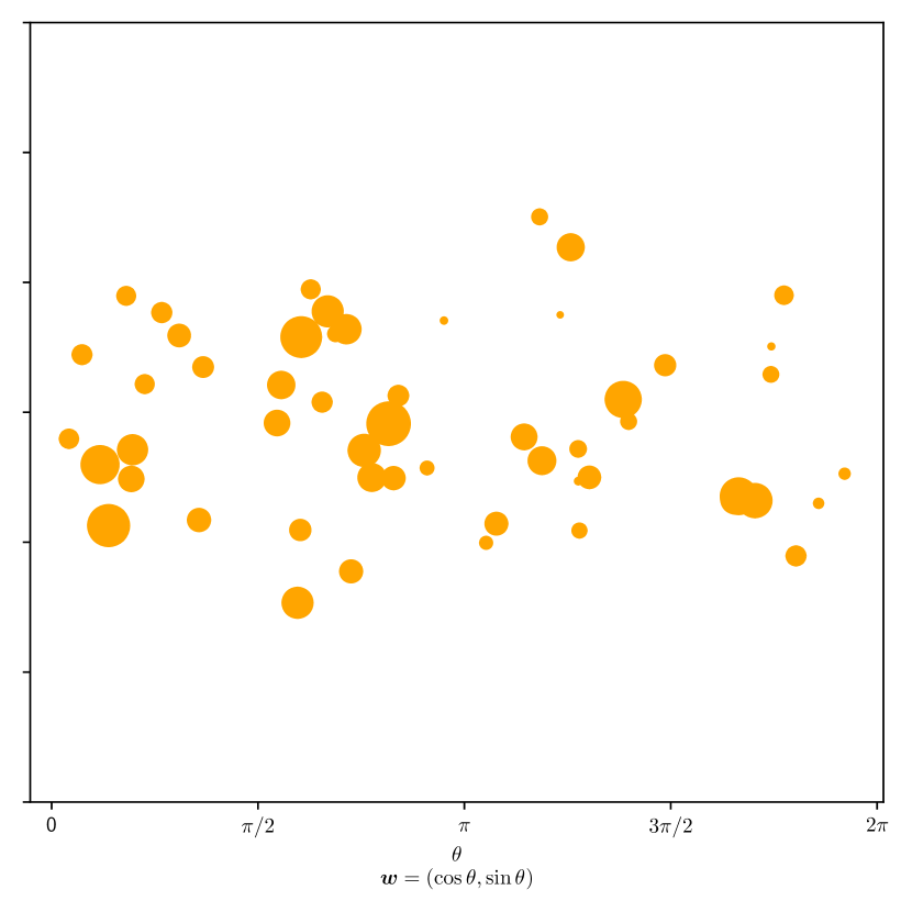
(d) $f_{2}$ trained without weight decay

Figure 2: We train a two output two-dimensional ReLU neural network of the form $f(x)=\sum_{k=1}^{K}{\bm{v}}_{k}\sigma({\bm{w}}^{T}_{k}{\bm{x}}+b_{k})$ both with and without weight decay. We plot the location of the active neurons contributing to each of the outputs of the network where the size of the point indicates the weight of the neuron. The figures in (a-b) show the neuron locations/weight for the network trained with weight decay whereas (c-d) shows the neuron locations/weight for the network trained without weight decay. We see that in the case of weight decay, we have fewer active neurons, and those neurons that remain are shared across both outputs.

4.2 Multi-Task Lasso Experiments

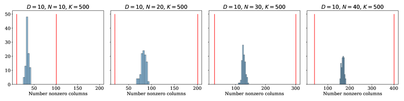
Figure 3: Distribution of the number of active columns for the solutions to the multi-task lasso problem on randomly generated matrices of varying sizes. In all these cases $r_{\mathbf{\Phi}}=N$ and $r_{\mathbf{\Psi}}=D$ so we expect $N\leq\widehat{K}\leq ND$. The red lines indicate the bounds from Theorem 12. The wide gap suggests that our upper bound can be tightened.

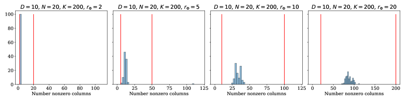
Figure 4: Distribution of the number of active columns for the solutions to the multi-task lasso problem on randomly generated matrices of varying sizes. In this case, we have that $\mathbf{\Phi}$ is low rank while $\mathbf{\Psi}$ remains at a rank of $D$. The red lines indicate the bounds from Theorem 12

We solve the multi-task lasso problem in Theorem 12 on randomly generated matrices $\mathbf{\Phi}$ and $\mathbf{\Psi}$ using CVXPy (Diamond and Boyd, 2016). Our experiments illustrate that while our bounds hold, the exact number of nonzero columns depends heavily on the data itself. In Figure (3) we show histograms for the distribution of non-zero columns over 100 randomly generated pairs of $\mathbf{\Phi}$ and $\mathbf{\Psi}$.

We perform a similar set of experiments in Figure (4) but alter the underlying rank of $\mathbf{\Phi}$. This validates our bound showing that the sparsity of the solution can be much lower depending on the rank of $\mathbf{\Phi}$. We again see that the distribution is highly dependent on the data and difficult to predict exactly. We note however that we never achieve our upper bound which may indicate that they can be further tightened.

To demonstrate that the sparsest solutions to the multi-task lasso problem in Theorem (12) depends heavily on the data matrices $\mathbf{\Phi}$ and $\mathbf{\Psi}$ we also ran a small-scale experiment similar to the one in 4.2. However, in these experiments, we exhaustively searched over all $2^{K}$ sparsity patterns that the solution may have. We arrive at the same conclusion as we did in 4.2 observing that the sparsest solution can lie anywhere within our bound as shown in Figure (5).

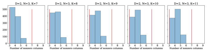
Figure 5: Distribution of number of nonzero columns for the solutions to the multi-task lasso problem. We ran this experiment over 1000 randomly generated matrices $\mathbf{\Phi}$ and $\mathbf{\Psi}$. We see that the sparsest solution is dependent on the data and can vary between our bounds. The red lines indicate the bounds from Theorem 12

4.3 Experiments Compressing pre-trained DNNs

As a practical application of our theory we conduct experiments compressing real deep neural networks pre-trained on the CIFAR-10 dataset. We first consider a pre-trained VGG19 architecture trained with weight decay. This model consists of various convolutional and batch norm layers followed by a fully connected ReLU layer containing 512 neurons.

The output of this layer is $\mathbf{\Psi}\in\mathbb{R}^{10\times N}$ due to having just 10 classes and therefore $\text{rank}(\mathbf{\Psi})\leq 10$. Moreover, we found that for the post-activation feature representation at this layer the first 10 singular values account for 99% of the energy of the signal (Figure 6), thus $\text{rank}({\mathbf{\Phi}})\approx 10$. Therefore, our bounds suggest that there exists an alternative optimal representation that is exactly equivalent on the training data, with no more than $100$ neurons in this layer. We validate this by applying the multi-task lasso problem (30) on the last fully connected ReLU layer. The results in Table 1 show that we can compress the final ReLU layer down to just 47 neurons while preserving nearly the same loss on the training data and achieving the same generalization performance.

Next, we consider the AlexNet architecture which is also composed of multiple convolutional layers followed by three fully connected ReLU layers with 9216, 4096, and 4096 neurons. We apply our multi-task lasso optimization to compress each of these layers in a parallel fashion and report the training loss and test accuracy with the compressed layers replaced individually and all at once. The results are on Table 1. For all four cases, we notice almost no change in the training loss and even better accuracy on the test data in some cases. This is due to the fact that our constraint only enforces that the network remains the same on the training data, while it may behave differently on data it was not trained on. Finally, we highlight that in all these cases no retraining is required to achieve comparable performance.

The minor discrepancies between the training losses of the original models and the compressed models are due to numerical issues when practically enforcing the constraint in in (28). In practice the constraint in (28) is approximated by formulating the solving the regularized version of the problem (35) and optimizing using proximal gradient descent. These results show us that our connection between weight decay and the multi-task lasso problem can hint at a principled approach to model compression that is also computationally efficient.

$$\min_{\{{\bm{v}}_{k}\}}\|\mathbf{V}\mathbf{\Phi}-\mathbf{\Psi}\|^{2}_{2}+\lambda\sum_{k=1}^{K}\|{\bm{v}}_{k}\|_{2}$$ (35)

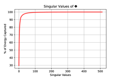
Figure 6: Cumulative plot of the singular values of the post-activation feature representations of the last layer of a pre-trained VGG19 on the entire CIFAR-10 dataset. We see that a large majority of the signal is captured by just the first few singular values, indicating that the representations are approximately low rank.

Table 1: Compressing Models Pre-trained on CIFAR-10

Network Name	Original Width	New Width	Orig. Train Loss (Test Acc.)	New Training Loss (Test Acc.)
VGG-19 (last layer)	512	47	0.0104 (93.92%)	0.0112 (93.88%)
AlexNet (last layer)	4096	797	0.2203 (72.17%)	0.2213 (72.22%)
AlexNet (penultimate layer)	4096	677	0.2203 (72.17%)	0.2184 (72.48%)
AlexNet (first linear layer)	9216	4896	0.2203 (72.17%)	0.2325 (72.28%)
AlexNet (last 3 layers)	(4096,4096,9216)	(797,677,4896)	0.2203 (72.17%)	0.2417(72.02%)

5 Related Works

In this section, we highlight some related works and discuss how our work fits into the current literature.

Variation Spaces and Representer Theorems for NNs.

Understanding NNs by studying the variation space associated with taking their widths to infinity has been explored in the past (Kurková and Sanguineti, 2001; Mhaskar, 2004; Bach, 2017). Representer theorems for showing that finite width networks are solutions to variational data-fitting problems posed over these spaces have also been developed (Parhi and Nowak, 2021, 2022; Unser, 2023; Bartolucci et al., 2023). However, most of these were restricted in that they only develop theories for shallow and scalar output NNs. Moreover, the norm associated with these variation spaces does not always coincide with regularizers used in practice such as weight decay. We are the first to study the $\mathcal{V}(\mathbb{R}^{d};\mathbb{R}^{D})$-space and develop a novel representer theorem for variational problems posed over such vector-valued function spaces.

Weight Decay and Width.

Numerous works have observed that weight decay is biased towards solutions with fewer neurons  (Savarese et al., 2019; Ongie et al., 2020; Parhi and Nowak, 2021; Yang et al., 2022). Empirically, Yang et al. (2022) showed that training NNs with weight decay for many iterations induces sparsity on the neurons of the network. Moreover, Jacot et al. (2022); Parhi and Nowak (2021) provide bounds on the required width for a DNNs that solve the weight decay objective. Our bounds improve upon the ones presented in both of these works. Moreover, our setting is a more general one, instead of only considering homogeneous DNNs our theory holds for the homogeneous layers of any DNN architecture. Recently, a line of work by Ergen and Pilanci (2021); Mishkin et al. (2022) has shown that training shallow ReLU NNs with weight decay can be recast as a convex program. Their reformulation reveals a sparse regularizer showing how weight decay induces solutions with few neurons. A similar observation was later extended to vector-valued neural networks in Sahiner et al. (2021).

Low-Rank Features.

It has been observed that DNNs are biased toward learning low-rank features. This has been shown to be true in theory (Du et al., 2018; Le and Jegelka, 2022; Ji and Telgarsky, 2019) for scalar output linear and nonlinear NNs. Moreover, Radhakrishnan et al. (2021) extended the theory for vector-valued linear NNs. Empirical evidence has also shown that the internal representations of deep neural networks are low rank (Huh et al., 2023; Nar et al., 2019; Waleffe and Rekatsinas, 2022). (Huh et al., 2023; Nar et al., 2019). In particular, Waleffe and Rekatsinas (2022) observe that the effective dimensions of hidden post-activation feature embeddings of trained NNs are often much smaller than the actual layer width. The authors utilize this insight to reduce the number of parameters using principal component analysis during training. In contrast, our theory and experiments indicate that narrower networks can be found without complicated procedures during training by instead applying the multi-task lasso as in Section 3.1.

6 Conclusion and Future Work

In this work we proposed the VV function space which gives insight into the type of NNs solutions that weight decay encourages. Moreover, we proved a new representer theorem for this space showing that finite-width vector-valued NNs are solutions to the variational data-fitting problem over this space. We then developed a novel connection between training DNNs with weight decay and multi-task lasso to prove the sharpest known bounds on network widths. Finally, we presented some experimental results showing the validity and potential utility of our theory.

Acknowledgments and Disclosure of Funding

The authors thank Ryan Tibshirani for helpful discussions regarding the lasso and related methods, especially the use of Carathéodory’s theorem for characterizing the sparsity of solutions. JS was supported by the ONR MURI grant N00014-20-1-2787. RP was supported by the European Research Council (ERC Project FunLearn) under grant 101020573. KL was supported by the NSF grant DMS-2023239. RN was supported in part by the NSF grants DMS-2134140 and DMS-2023239, the ONR MURI grant N00014-20-1-2787, and the AFOSR/AFRL grant FA9550-18-1-0166, as well as the Keith and Jane Nosbusch Professorship.

Appendix A Proof of Lemma 4

We prove the following result which corresponds to Lemma 4 by choosing $\Omega=\mathbb{S}^{d}$.

Lemma 15

Let $\Omega$ be any locally compact Hausdorff space. The norms $\lVert\mkern 1.0mu\cdot\mkern 1.0mu\rVert_{p,\mathcal{M}}$, $p\geq 1$, and $\lVert\mkern 1.0mu\cdot\mkern 1.0mu\rVert_{\mathcal{M},q}$, $q\geq 1$ (appropriately defined on $\mathcal{M}(\Omega;\mathbb{R}^{D})$) are all equivalent Banach norms for $\mathcal{M}(\Omega;\mathbb{R}^{D})$.

Proof  We first observe that for any $p,q\geq 1$, the norms $\lVert\mkern 1.0mu\cdot\mkern 1.0mu\rVert_{\mathcal{M},p}$ and $\lVert\mkern 1.0mu\cdot\mkern 1.0mu\rVert_{\mathcal{M},q}$ are equivalent by the equivalence of $p$-norms in finite dimensions. Similarly, for any $p,q\geq 1$, the norms $\lVert\mkern 1.0mu\cdot\mkern 1.0mu\rVert_{p,\mathcal{M}}$ and $\lVert\mkern 1.0mu\cdot\mkern 1.0mu\rVert_{q,\mathcal{M}}$ are equivalent. Thus, it suffices to show that $\lVert\mkern 1.0mu\cdot\mkern 1.0mu\rVert_{\mathcal{M},p}$ and $\lVert\mkern 1.0mu\cdot\mkern 1.0mu\rVert_{q,\mathcal{M}}$ are equivalent for some $p,q\geq 1$.

We have for any ${\bm{\nu}}\in\mathcal{M}(\Omega;\mathbb{R}^{D})$

$$\lVert{\bm{\nu}}\rVert_{\mathcal{M},1} =\sum_{j=1}^{D}\lVert\nu_{j}\rVert_{\mathcal{M}(\Omega)}$$

$$=\sum_{j=1}^{D}\sup_{\begin{subarray}{c}\Omega=\bigcup_{i=1}^{n}A_{i}\\ n\in\mathbb{N}\end{subarray}}\sum_{i=1}^{n}\lvert\nu_{j}(A_{i})\rvert$$

$$\geq\sup_{\begin{subarray}{c}\Omega=\bigcup_{i=1}^{n}A_{i}\\ n\in\mathbb{N}\end{subarray}}\sum_{j=1}^{D}\sum_{i=1}^{n}\lvert\nu_{j}(A_{i})\rvert$$

$$=\sup_{\begin{subarray}{c}\Omega=\bigcup_{i=1}^{n}A_{i}\\ n\in\mathbb{N}\end{subarray}}\sum_{i=1}^{n}\sum_{j=1}^{D}\lvert\nu_{j}(A_{i})\rvert$$

$$=\sup_{\begin{subarray}{c}\Omega=\bigcup_{i=1}^{n}A_{i}\\ n\in\mathbb{N}\end{subarray}}\sum_{i=1}^{n}\lVert{\bm{\nu}}(A_{i})\rVert_{1}=\lVert{\bm{\nu}}\rVert_{1,\mathcal{M}}.$$ (36)

Since the inclusion/identity map

$$\iota:(\mathcal{M}(\Omega;\mathbb{R}^{D}),\lVert\mkern 1.0mu\cdot\mkern 1.0mu\rVert_{\mathcal{M},1})\to(\mathcal{M}(\Omega;\mathbb{R}^{D}),\lVert\mkern 1.0mu\cdot\mkern 1.0mu\rVert_{1,\mathcal{M}})$$

is obviously a bijection and satisfies the continuity bound Eq. 36, the bounded inverse theorem (Folland, 1999, Corollary 5.11) guarantees that the inverse $\iota^{-1}$ is also bounded. In other words, there exists a constant $C>0$ (which may depend on $\Omega$ and $D$) such that for all ${\bm{\nu}}\in\mathcal{M}(\Omega;\mathbb{R}^{D})$,

$$\lVert{\bm{\nu}}\rVert_{\mathcal{M},1}=\lVert\iota^{-1}{\bm{\nu}}\rVert_{\mathcal{M},1}\leq C\lVert{\bm{\nu}}\rVert_{1,\mathcal{M}}.$$

Therefore, we have shown that $\lVert\mkern 1.0mu\cdot\mkern 1.0mu\rVert_{\mathcal{M},1}$ and $\lVert\mkern 1.0mu\cdot\mkern 1.0mu\rVert_{1,\mathcal{M}}$ are equivalent, which proves the lemma.  

A.1 Connection to the Total Variation of Function

The total variation of a measure is different than the total variation of a function, but the ideas are tightly linked. In the univariate case, consider a Radon measure $\mu\in\mathcal{M}(\mathbb{R})$ and suppose there exists a function $g_{\mu}:\mathbb{R}\to\mathbb{R}$ such that

$$\int_{\mathbb{R}}f(x)\,\mathrm{d}\mu(x)=\int_{\mathbb{R}}f(x)\,\mathrm{d}g_{\mu}(x),$$

where $f$ is any bounded continuous function and the integral on the right-hand side is a Riemann–Stieltjes integral. If $g_{\mu}$ is differentiable and its derivative, denoted by $g_{\mu}^{\prime}$, is in $L^{1}(\mathbb{R})$, then we have the equality

$$\lVert\mu\rVert_{\mathcal{M}(\mathbb{R})}=\lVert g_{\mu}^{\prime}\rVert_{L^{1}(\mathbb{R})}.$$

The quantity on the right-hand side is referred to as the total variation of the function $g_{\mu}$. Furthermore, if $g_{\mu}$ is not differentiable in the classical sense, its distributional derivative can be identified with the Radon measure $\mu$, i.e., $g_{\mu}^{\prime}=\mu$, where equality is understood in $\mathcal{M}(\mathbb{R})$. In this case, $\lVert g_{\mu}^{\prime}\rVert_{\mathcal{M}(\mathbb{R})}=\lVert\mu\rVert_{\mathcal{M}(\mathbb{R})}$ is the total variation of the function $g_{\mu}$.

This correspondence extends to higher dimensions. Indeed, given a function $g:\mathbb{R}^{d}\to\mathbb{R}$, if its distributional gradient $\nabla g$ can be identified with a vector-valued finite Radon measure, then the isotropic total variation of $g$ is

$$\operatorname{TV}_{\mathrm{iso}}(g)\coloneqq\lVert\nabla g\rVert_{2,\mathcal{M}},$$

while the anisotropic total variation of $g$ is

$$\operatorname{TV}_{\mathrm{aniso}}(g)\coloneqq\lVert\nabla g\rVert_{1,\mathcal{M}}.$$

These two notions of total variation in multiple dimensions are often used in image processing problems. Finally, the isotropic total variation is equivalently specified by

$$\operatorname{TV}_{\mathrm{iso}}(g)=\sup_{\begin{subarray}{c}\varphi\in\mathcal{D}(\mathbb{R}^{d};\mathbb{R}^{d})\\ \lVert\varphi\rVert_{L^{\infty}(\mathbb{R}^{d};\mathbb{R}^{d})}=1\end{subarray}}\int_{\mathbb{R}^{d}}g({\bm{x}})\,\mathrm{div}\varphi({\bm{x}})\,\mathrm{d}{\bm{x}},$$

where the $L^{\infty}(\mathbb{R}^{d};\mathbb{R}^{d})$-norm is specified by

$$\lVert\varphi\rVert_{L^{\infty}(\mathbb{R}^{d};\mathbb{R}^{d})}\coloneqq\operatorname*{ess\,sup}_{{\bm{x}}\in\mathbb{R}^{d}}\>\lVert\varphi({\bm{x}})\rVert_{2},$$

and $\mathcal{D}(\mathbb{R}^{d};\mathbb{R}^{d})$ denotes the space of infinitely differentiable compactly supported functions mapping $\mathbb{R}^{d}\to\mathbb{R}^{d}$. We refer the reader to the book of Evans and Gariepy (2015) for more details about the total variation of a function.

Appendix B Proof of Theorem 5

Proof  From the definition of the $\mathcal{V}(\mathbb{R}^{d};\mathbb{R}^{D})$-norm Eq. 15, it follows from a standard argument (cf., Bartolucci et al., 2023, Proposition 3.7) that the problem in Eq. 18 is equivalent to the problem

$$\inf_{{\bm{\nu}}\in\mathcal{M}(\mathbb{S}^{d};\mathbb{R}^{D})}\>\sum_{i=1}^{N}\mathcal{L}\left({\bm{y}}_{i},\int_{\mathbb{S}^{d}}\sigma({\bm{w}}^{T}\overline{{\bm{x}}}_{i})\,\mathrm{d}{\bm{\nu}}({\bm{w}})\right)+\lambda\lVert{\bm{\nu}}\rVert_{2,\mathcal{M}}$$ (37)

in the sense that their infimal values are the same and if ${\bm{\nu}}^{\star}$ is a solution to Eq. 37, then

$$f_{{\bm{\nu}}^{\star}}({\bm{x}})=\int_{\mathbb{S}^{d}}\sigma({\bm{w}}^{T}\overline{{\bm{x}}}_{i})\,\mathrm{d}{\bm{\nu}}^{\star}({\bm{w}})$$

is a solution to Eq. 18. We now proceed in four steps to prove the theorem.

Step (i): Existence of solutions to Eq. 37.

Define

$$\mathcal{J}({\bm{\nu}})\coloneqq\sum_{i=1}^{N}\mathcal{L}\left({\bm{y}}_{i},\int_{\mathbb{S}^{d}}\sigma({\bm{w}}^{T}\overline{{\bm{x}}}_{i})\,\mathrm{d}{\bm{\nu}}({\bm{w}})\right)+\lambda\lVert{\bm{\nu}}\rVert_{2,\mathcal{M}}$$

Given an arbitrary ${\bm{\nu}}_{0}\in\mathcal{M}(\mathbb{S}^{d};\mathbb{R}^{D})$, let $C_{0}\coloneqq\mathcal{J}({\bm{\nu}}_{0})$. Then, we can transform Eq. 37 into the constrained problem

$$\inf_{{\bm{\nu}}\in\mathcal{M}(\mathbb{S}^{d};\mathbb{R}^{D})}\>\mathcal{J}({\bm{\nu}})\quad\textrm{s.t.}\quad\lVert{\bm{\nu}}\rVert_{2,\mathcal{M}}\leq C_{0}/\lambda.$$ (38)

This transformation is valid since any measure that does not satisfy the constraint will have an objective value strictly larger than ${\bm{\nu}}_{0}$ and therefore will not be in the solution set. Next, we note that we can write

$$\mathcal{J}({\bm{\nu}})=\sum_{i=1}^{N}\mathcal{L}\left({\bm{y}}_{i},\operatorname{H}_{i}\{{\bm{\nu}}\}\right)+\lambda\lVert{\bm{\nu}}\rVert_{2,\mathcal{M}}$$

where

$$\operatorname{H}_{i}\{{\bm{\nu}}\}\coloneqq\begin{bmatrix}\langle{\bm{\nu}},h_{i,j}\rangle\\ \vdots\\ \langle{\bm{\nu}},h_{i,D}\rangle\end{bmatrix}\in\mathbb{R}^{D}$$ (39)

with $h_{i,j}({\bm{w}})\coloneqq\sigma({\bm{w}}^{T}\overline{{\bm{x}}}_{i}){\bm{e}}_{j}$, where ${\bm{e}}_{j}\in\mathbb{R}^{D}$ is the $j$th canonical unit vector. Clearly $h_{i,j}\in C(\mathbb{S}^{d};\mathbb{R}^{D})$, the space of continuous functions on $\mathbb{S}^{d}$ taking values in $\mathbb{R}^{D}$. In Eq. 39, $\langle\mkern 1.0mu\cdot\mkern 1.0mu,\mkern 1.0mu\cdot\mkern 1.0mu\rangle$ denotes the duality pairing between $C(\mathbb{S}^{d};\mathbb{R}^{D})$ and $\mathcal{M}(\mathbb{S}^{d};\mathbb{R}^{D})$. Thus, for $i=1,\ldots,N$, $\operatorname{H}_{i}$ is component-wise weak^∗ continuous on $\mathcal{M}(\mathbb{S}^{d};\mathbb{R}^{D})$. Since $\mathcal{L}(\mkern 1.0mu\cdot\mkern 1.0mu,\mkern 1.0mu\cdot\mkern 1.0mu)$ is lower semicontinuous in its second argument combined with the fact that every norm is weak^∗ continuous on its corresponding Banach space, we have that $\mathcal{J}$ is weak^∗ continuous on $\mathcal{M}(\mathbb{S}^{d};\mathbb{R}^{D})$. By the Banach–Alaoglu theorem (Rudin, 1991, Chapter 3), the constraint set of Eq. 38 is weak^∗ compact. Thus, Eq. 38 is the minimization of a weak^∗ continuous functional over a weak^∗ compact set. By the Weierstrass extreme value theorem on general topological spaces (Kurdila and Zabarankin, 2006, Chapter 5), there exists a solution to (38) (and subsequently of (37)).

Step (ii): Recasting Eq. 37 as an interpolation problem.

Let $\widetilde{{\bm{\nu}}}$ be a (not neccesarily unique) solution to Eq. 37, which is guaranteed to exist by the previous argumentation. For $i=1,\ldots,D$, define

$${\bm{z}}_{i}=\operatorname{H}_{i}\{\widetilde{{\bm{\nu}}}\}\in\mathbb{R}^{D}.$$

Then, $\widetilde{{\bm{\nu}}}$ must satisfy

$$\widetilde{{\bm{\nu}}}\in\operatorname*{arg\,min}_{{\bm{\nu}}\in\mathcal{M}(\mathbb{S}^{d};\mathbb{R}^{D})}\lVert{\bm{\nu}}\rVert_{2,\mathcal{M}}\quad\textrm{s.t.}\quad\operatorname{H}_{i}\{{\bm{\nu}}\}={\bm{z}}_{i},\>i=1,\ldots,N.$$ (40)

To see this, we note that if this were not the case, it would contradict the optimality of $\widetilde{{\bm{\nu}}}$. This reduction implies that any solution to the interpolation problem Eq. 40 will also be a solution to Eq. 37.

Step (iii): The form of the solution.

We can rewrite the interpolation problem as

$$\min_{{\bm{\nu}}\in\mathcal{M}(\mathbb{S}^{d};\mathbb{R}^{D})}\lVert{\bm{\nu}}\rVert_{2,\mathcal{M}}\quad\textrm{s.t.}\quad\langle{\bm{\nu}},h_{i,j}\rangle={\bm{z}}_{i,j},\>i=1,\ldots,N\text{ and }j=1,\ldots,D.$$ (41)

This is the vector-valued analogue of the classical (Radon) measure recovery problem with $ND$ weak^∗ continuous measurements. By the abstract representer theorem of Unser (2021, Theorems 2 and 3) (see also Boyer et al., 2019; Bredies and Carioni, 2020), there always exists a solution to Eq. 41 that takes the form

$${\bm{\nu}}^{\star}=\sum_{k=1}^{K}c_{k}{\bm{e}}_{k}$$

with $K\leq ND$, $c_{k}\in\mathbb{R}\setminus\{0\}$ where for $k=1,\ldots,k$, ${\bm{e}}_{k}$ is an extreme point of the unit regularization ball

$$B\coloneqq\{{\bm{\nu}}\in\mathcal{M}(\mathbb{S}^{d};\mathbb{R}^{D})\>\colon\>\lVert{\bm{\nu}}\rVert_{2,\mathcal{M}}\leq 1\}.$$

From Werner (1984, Theorem 2), the extreme points of $B$ take the form ${\bm{a}}\delta_{\bm{w}}$ with ${\bm{a}}\in\mathbb{R}^{D}$, $\lVert{\bm{a}}\rVert_{2}=1$, and ${\bm{w}}\in\mathbb{S}^{d}$. Thus, we can write

$${\bm{\nu}}^{\star}=\sum_{k=1}^{K}c_{k}{\bm{a}}_{k}\delta_{{\bm{w}}_{k}}$$

with ${\bm{a}}_{k}\in\mathbb{R}^{D}$ and ${\bm{w}}_{k}\in\mathbb{S}^{d}$. By the equivalence between Eq. 37 and Eq. 18, we find that there exists a solution to Eq. 18 that takes the form

$$\widehat{f}({\bm{x}})=\sum_{k=1}^{\widehat{K}}\widehat{{\bm{v}}}_{k}\sigma(\widehat{{\bm{w}}}_{k}^{T}\overline{{\bm{x}}}),\quad{\bm{x}}\in\mathbb{R}^{d},$$

where $\widehat{K}\leq ND$, $\widehat{{\bm{v}}}_{k}\coloneqq c_{k}{\bm{a}}_{k}\in\mathbb{R}^{D}$ and $\widehat{{\bm{w}}}_{k}\in\mathbb{S}^{d}$.

Step (iv): Sharpening the sparsity bound.

Step (iii) establishes that there exists an optimal solution with $\widehat{K}\leq ND$ neurons. Thus, we can apply Theorem 9 to find another solution where the number of neurons is bounded by the product of the rank of the labels $\mathbf{Y}\in\mathbb{R}^{D\times N}$ with the rank of the post-activation feature matrix $\mathbf{\Phi}\in\mathbb{R}^{\widehat{K}\times N}$. From the dimensions of these matrices, we see that the product of the ranks is $\leq N^{2}$. Thus, by Theorem 9, there exists a solution to Eq. 18 that takes the form

$$f^{\star}({\bm{x}})=\sum_{k=1}^{K_{0}}{\bm{v}}_{k}\sigma({\bm{w}}_{k}^{T}\overline{{\bm{x}}}),\quad{\bm{x}}\in\mathbb{R}^{d},$$

where $K_{0}\leq N^{2}$, ${\bm{v}}_{k}\in\mathbb{R}^{D}$ and ${\bm{w}}_{k}\in\mathbb{S}^{d}$. Thus, we can always find a solution to Eq. 18 with $\min\{N^{2},ND\}$ neurons.

References

• Argyriou et al. (2008) A. Argyriou, T. Evgeniou, and M. Pontil. Convex multi-task feature learning. Machine learning, 73:243–272, 2008.
• Bach (2017) F. Bach. Breaking the curse of dimensionality with convex neural networks. The Journal of Machine Learning Research, 18(1):629–681, 2017.
• Barron (1993) A. R. Barron. Universal approximation bounds for superpositions of a sigmoidal function. IEEE Transactions on Information Theory, 39(3):930–945, 1993.
• Bartlett (1996) P. Bartlett. For valid generalization the size of the weights is more important than the size of the network. Advances in Neural Information Processing Systems, 9, 1996.
• Bartolucci et al. (2023) F. Bartolucci, E. De Vito, L. Rosasco, and S. Vigogna. Understanding neural networks with reproducing kernel Banach spaces. Appl. Comput. Harmon. Anal., 62:194–236, 2023.
• Bengio et al. (2005) Y. Bengio, N. Roux, P. Vincent, O. Delalleau, and P. Marcotte. Convex neural networks. Advances in Neural Information Processing Systems, 18, 2005.
• Bos and Chug (1996) S. Bos and E. Chug. Using weight decay to optimize the generalization ability of a perceptron. In Proceedings of International Conference on Neural Networks (ICNN’96), volume 1, pages 241–246. IEEE, 1996.
• Boyer et al. (2019) C. Boyer, A. Chambolle, Y. De Castro, V. Duval, F. de Gournay, and P. Weiss. On representer theorems and convex regularization. SIAM J. Optim., 29(2):1260–1281, 2019. ISSN 1052-6234.
• Bredies and Carioni (2020) K. Bredies and M. Carioni. Sparsity of solutions for variational inverse problems with finite-dimensional data. Calc. Var. Partial Differential Equations, 59(1):Paper No. 14, 26, 2020. ISSN 0944-2669.
• Bredies and Holler (2020) K. Bredies and M. Holler. Higher-order total variation approaches and generalisations. Inverse Problems, 36(12):123001, 2020.
• Clarke (2013) F. Clarke. Functional analysis, calculus of variations and optimal control, volume 264. Springer, 2013.
• Diamond and Boyd (2016) S. Diamond and S. Boyd. Cvxpy: A python-embedded modeling language for convex optimization. The Journal of Machine Learning Research, 17(1):2909–2913, 2016.
• Diestel and Uhl (1977) J. Diestel and J. Uhl. Vector Measures. Mathematical surveys and monographs. American Mathematical Society, 1977. ISBN 9780821815151.
• Du et al. (2018) S. S. Du, W. Hu, and J. D. Lee. Algorithmic regularization in learning deep homogeneous models: Layers are automatically balanced. Advances in Neural Information Processing Systems, 31, 2018.
• Ergen and Pilanci (2021) T. Ergen and M. Pilanci. Convex geometry and duality of over-parameterized neural networks. Journal of Machine Learning Research, 2021.
• Evans and Gariepy (2015) L. C. Evans and R. F. Gariepy. Measure theory and fine properties of functions. CRC press, 2015.
• Folland (1999) G. B. Folland. Real analysis: modern techniques and their applications, volume 40. John Wiley & Sons, 1999.
• Grandvalet (1998) Y. Grandvalet. Least absolute shrinkage is equivalent to quadratic penalization. In International Conference on Artificial Neural Networks, pages 201–206. Springer, 1998.
• Hensgen (1996) W. Hensgen. A simple proof of Singer’s representation theorem. Proceedings of the American Mathematical Society, 124(10):3211–3212, 1996.
• Huh et al. (2023) M. Huh, H. Mobahi, R. Zhang, B. Cheung, P. Agrawal, and P. Isola. The low-rank simplicity bias in deep networks. Transactions on Machine Learning Research, 2023. ISSN 2835-8856. URL https://openreview.net/forum?id=bCiNWDmlY2.
• Jacot (2023) A. Jacot. Implicit bias of large depth networks: a notion of rank for nonlinear functions. In The Eleventh International Conference on Learning Representations, 2023. URL https://openreview.net/forum?id=6iDHce-0B-a.
• Jacot et al. (2022) A. Jacot, E. Golikov, C. Hongler, and F. Gabriel. Feature learning in $l_{2}$-regularized DNNs: Attraction/repulsion and sparsity. In A. H. Oh, A. Agarwal, D. Belgrave, and K. Cho, editors, Advances in Neural Information Processing Systems, 2022. URL https://openreview.net/forum?id=kK200QKfvjB.
• Ji and Telgarsky (2019) Z. Ji and M. Telgarsky. Gradient descent aligns the layers of deep linear networks. In International Conference on Learning Representations, 2019. URL https://openreview.net/forum?id=HJflg30qKX.
• Jones (1992) L. K. Jones. A simple lemma on greedy approximation in Hilbert space and convergence rates for projection pursuit regression and neural network training. The Annals of Statistics, pages 608–613, 1992.
• Kolesnikov et al. (2020) A. Kolesnikov, L. Beyer, X. Zhai, J. Puigcerver, J. Yung, S. Gelly, and N. Houlsby. Big transfer (bit): General visual representation learning. In European conference on computer vision, pages 491–507. Springer, 2020.
• Korolev (2022) Y. Korolev. Two-layer neural networks with values in a Banach space. SIAM Journal on Mathematical Analysis, 54(6):6358–6389, 2022.
• Krizhevsky et al. (2017) A. Krizhevsky, I. Sutskever, and G. E. Hinton. Imagenet classification with deep convolutional neural networks. Communications of the ACM, 60(6):84–90, 2017.
• Krogh and Hertz (1991) A. Krogh and J. Hertz. A simple weight decay can improve generalization. Advances in Neural Information Processing Systems, 4, 1991.
• Kunin et al. (2021) D. Kunin, J. Sagastuy-Brena, S. Ganguli, D. L. Yamins, and H. Tanaka. Neural mechanics: Symmetry and broken conservation laws in deep learning dynamics. In International Conference on Learning Representations, 2021. URL https://openreview.net/forum?id=q8qLAbQBupm.
• Kurdila and Zabarankin (2006) A. J. Kurdila and M. Zabarankin. Convex Functional Analysis. Systems & Control: Foundations & Applications. Birkhäuser Basel, 2006.
• Kurková and Sanguineti (2001) V. Kurková and M. Sanguineti. Bounds on rates of variable-basis and neural-network approximation. IEEE Transactions on Information Theory, 47(6):2659–2665, 2001.
• Le and Jegelka (2022) T. Le and S. Jegelka. Training invariances and the low-rank phenomenon: beyond linear networks. In International Conference on Learning Representations, 2022. URL https://openreview.net/forum?id=XEW8CQgArno.
• Mhaskar (2004) H. N. Mhaskar. On the tractability of multivariate integration and approximation by neural networks. Journal of Complexity, 20(4):561–590, 2004.
• Mishkin et al. (2022) A. Mishkin, A. Sahiner, and M. Pilanci. Fast convex optimization for two-layer relu networks: Equivalent model classes and cone decompositions. In International Conference on Machine Learning, 2022.
• Nar et al. (2019) K. Nar, O. Ocal, S. S. Sastry, and K. Ramchandran. Cross-entropy loss leads to poor margins, 2019. URL https://openreview.net/forum?id=ByfbnsA9Km.
• Neyshabur et al. (2015) B. Neyshabur, R. R. Salakhutdinov, and N. Srebro. Path-SGD: Path-normalized optimization in deep neural networks. Advances in Neural Information Processing Systems, 28, 2015.
• Obozinski et al. (2006) G. Obozinski, B. Taskar, and M. Jordan. Multi-task feature selection. Statistics Department, UC Berkeley, Tech. Rep, 2(2.2):2, 2006.
• Obozinski et al. (2010) G. Obozinski, B. Taskar, and M. I. Jordan. Joint covariate selection and joint subspace selection for multiple classification problems. Statistics and Computing, 20:231–252, 2010.
• Ongie et al. (2020) G. Ongie, R. Willett, D. Soudry, and N. Srebro. A function space view of bounded norm infinite width ReLU nets: The multivariate case. In International Conference on Learning Representations, 2020.
• Papyan et al. (2020) V. Papyan, X. Han, and D. L. Donoho. Prevalence of neural collapse during the terminal phase of deep learning training. Proceedings of the National Academy of Sciences, 117(40):24652–24663, 2020.
• Parhi and Nowak (2020) R. Parhi and R. D. Nowak. The role of neural network activation functions. IEEE Signal Processing Letters, 27:1779–1783, 2020.
• Parhi and Nowak (2021) R. Parhi and R. D. Nowak. Banach space representer theorems for neural networks and ridge splines. The Journal of Machine Learning Research, 22(43):1–40, 2021.
• Parhi and Nowak (2022) R. Parhi and R. D. Nowak. What kinds of functions do deep neural networks learn? Insights from variational spline theory. SIAM Journal on Mathematics of Data Science, 4(2):464–489, 2022.
• Parhi and Nowak (2023a) R. Parhi and R. D. Nowak. Near-minimax optimal estimation with shallow ReLU neural networks. IEEE Transactions on Information Theory, 69(2):1125–1140, 2023a.
• Parhi and Nowak (2023b) R. Parhi and R. D. Nowak. Deep learning meets sparse regularization: A signal processing perspective. arXiv preprint arXiv:2301.09554, 2023b.
• Pisier (1981) G. Pisier. Remarques sur un résultat non publié de B. Maurey. Séminaire d’Analyse Fonctionnelle (dit “Maurey-Schwartz”), pages 1–12, April 1981.
• Power et al. (2021) A. Power, Y. Burda, H. Edwards, I. Babuschkin, and V. Misra. Grokking: Generalization beyond overfitting on small algorithmic datasets. 1st Mathematical Reasoning in General Artificial Intelligence Workshop ICLR, 2021.
• Radhakrishnan et al. (2021) A. Radhakrishnan, E. Nichani, D. Bernstein, and C. Uhler. On alignment in deep linear neural networks. ICML Workshop on Over-parameterization: Pitfalls and Opportunities, 2021.
• Rockafellar (1997) R. T. Rockafellar. Convex analysis, volume 11. Princeton university press, 1997.
• Rosset et al. (2007) S. Rosset, G. Swirszcz, N. Srebro, and J. Zhu. l1 regularization in infinite dimensional feature spaces. In COLT, pages 544–558. Springer, 2007.
• Rudin (1991) W. Rudin. Functional Analysis. International series in pure and applied mathematics. McGraw-Hill, 1991.
• Sahiner et al. (2021) A. Sahiner, T. Ergen, J. M. Pauly, and M. Pilanci. Vector-output relu neural network problems are copositive programs: Convex analysis of two layer networks and polynomial-time algorithms. In International Conference on Learning Representations, 2021. URL https://openreview.net/forum?id=fGF8qAqpXXG.
• Savarese et al. (2019) P. Savarese, I. Evron, D. Soudry, and N. Srebro. How do infinite width bounded norm networks look in function space? In Conference on Learning Theory, pages 2667–2690. PMLR, 2019.
• Shenouda and Bajwa (2023) J. Shenouda and W. U. Bajwa. A guide to computational reproducibility in signal processing and machine learning [tips & tricks]. IEEE Signal Processing Magazine, 40(2):141–151, 2023.
• Siegel and Xu (2023) J. W. Siegel and J. Xu. Characterization of the variation spaces corresponding to shallow neural networks. Constructive Approximation, pages 1–24, 2023.
• Simonyan and Zisserman (2014) K. Simonyan and A. Zisserman. Very deep convolutional networks for large-scale image recognition. CoRR, abs/1409.1556, 2014.
• Singer (1957) I. Singer. Linear functionals on the space of continuous mappings of a compact Hausdorff space into a Banach spaces. Rev. Math. Pures Appl., 2:301–315, 1957.
• Singer (1959) I. Singer. Sur les applications linéaires intégrales des espaces de fonctions continues. i. Rev. Math. Pures Appl, 4(1959):391–401, 1959.
• Tibshirani (2013) R. J. Tibshirani. The lasso problem and uniqueness. Electronic Journal of Statistics, 7:1456–1490, 2013.
• Triebel (1983) H. Triebel. Theory of Function Spaces. Monographs in Mathematics. Springer Basel, 1983. ISBN 9783764313814.
• Unser (2021) M. Unser. A unifying representer theorem for inverse problems and machine learning. Found. Comput. Math., 21(4):941–960, 2021. ISSN 1615-3375.
• Unser (2023) M. Unser. Ridges, neural networks, and the Radon transform. Journal of Machine Learning Research, 24(37):1–33, 2023.
• Waleffe and Rekatsinas (2022) R. Waleffe and T. Rekatsinas. Principal component networks: Parameter reduction early in training. Hardware Aware Efficient Training (HAET) Workshop at the 39th ICML, 2022.
• Wang et al. (2021) H. Wang, S. Agarwal, and D. Papailiopoulos. Pufferfish: communication-efficient models at no extra cost. Proceedings of Machine Learning and Systems, 3:365–386, 2021.
• Werner (1984) D. Werner. Extreme points in spaces of operators and vector–valued measures. Proceedings of the 12th Winter School on Abstract Analysis, pages 135–143, 1984.
• Yang et al. (2022) L. Yang, J. Zhang, J. Shenouda, D. Papailiopoulos, K. Lee, and R. D. Nowak. A better way to decay: Proximal gradient training algorithms for neural nets. In OPT 2022: Optimization for Machine Learning (NeurIPS Workshop), 2022.
• Zhai et al. (2019) X. Zhai, A. Oliver, A. Kolesnikov, and L. Beyer. S4l: Self-supervised semi-supervised learning. In Proceedings of the IEEE/CVF International Conference on Computer Vision, pages 1476–1485, 2019.
• Zhang et al. (2021) C. Zhang, S. Bengio, M. Hardt, B. Recht, and O. Vinyals. Understanding deep learning (still) requires rethinking generalization. Communications of the ACM, 64(3):107–115, 2021.