Two-photon double ionization with finite pulses:
Application of the virtual sequential model to helium

Abstract

As a step toward the full ab-initio description of two-photon double ionization processes, we present a finite-pulse version of the virtual-sequential model for polyelectronic atoms. The model relies on the ab initio description of the single ionization scattering states of both the neutral and ionized target system. As a proof of principle and a benchmark, the model is applied to the helium atom using the NewStock atomic photoionization code. The results of angularly integrated observables, which are in excellent agreement with existing TDSE (time-dependent Schrödinger equation) simulations, show how the model is able to capture the role of electron correlation in the non-sequential regime, and the influence of autoionizing states in the sequential regime, at a comparatively modest computational cost. The model also reproduces the two-particle interference with ultrashort pulses, which is within reach of current experimental technologies. Furthermore, the model shows the modulation of the joint energy distribution in the vicinity of autoionizing states, which can be probed with extreme-ultraviolet pulses of duration much longer than the characteristic lifetime of the resonance. The formalism discussed here applies also to polyelectronic atoms and molecules, thus opening a window on non-sequential and sequential double ionization in these more complex systems.

I Introduction

Our understanding of electron dynamics in atomic and molecular photoionization processes has drastically improved over the last two decades, driven by the rapid development of coherent extreme-ultraviolet (XUV) and x-ray light sources Corkum and Krausz (2007); Krausz and Ivanov (2009); Pazourek et al. (2015). Thanks to the increase in intensity of ionizing pulses at x-ray Free-Electron-Laser facilities (XFELs) as well as with table-top setups, the use of XUV-pump XUV-probe schemes to study unperturbed correlated electronic motion in real time is on the horizon Duris et al. (2020); Saito et al. (2019); Borrego-Varillas et al. (2022). In these studies, double ionization plays a central role both because of its unique sensitivity to electronic correlation and because it enables the detection of correlated electron pairs in coincidence Weber et al. (2000); Bergues et al. (2012); Månsson et al. (2014).

Extensive studies of two-photon double ionization (TPDI) in helium over the past two decades have substantially contributed to the understanding of correlated electron dynamics in atomic physics. Different regimes for the TPDI process contain detailed information on electron correlation-driven dynamics. In the sequential regime, a first photon ionizes the system, generating an intermediate ion, which subsequently absorbs a second photon, thus emitting a second electron. This mechanism, therefore, consists of two independent single photoionization events and it is active only if the absorbed photons are able to ionize the initial target and the residual ion. The sequential mechanism can be described, in its qualitative features, by an independent-particle model. In the non-sequential regime, the two photons are absorbed in too short a sequence for the system to settle down in a well-defined intermediate state. For this reason, this mechanism can lead to the concerted emission of two electrons even if the energy of a single photon is insufficient to ionize the parent ion, provided that the energy of the two photons together exceeds the double-ionization threshold.

Since the non-sequential mechanism relies on virtual intermediate states that can be achieved only through multiple single-electron excitations from the reference ground-state configuration, electron correlation plays an essential role in it and must be taken into account in the initial, intermediate, and final states. Indeed, several perturbative approaches based on lowest-order perturbation theory have demonstrated the role of electron correlation in the non-sequential regime Horner et al. (2007); Ivanov and Kheifets (2007); Horner et al. (2008a, b); Førre et al. (2010); Nikolopoulos and Lambropoulos (2001). Only direct numerical solutions of the time-dependent Schrödinger equation (TDSE), however, could settle the residual disputes on the quantitative aspects of this process even for a seemingly elementary system like the helium atom Feist et al. (2008); Foumouo et al. (2008); Palacios et al. (2008); Nepstad et al. (2010); Guan et al. (2008); Hu et al. (2004); Colgan and Pindzola (2002); Jiang et al. (2015). The quantitative description of TPDI dynamics entailed by pump-probe experiments requires expensive numerical simulations Feist et al. (2008); Palacios et al. (2008, 2009); Feist et al. (2009); Palacios et al. (2010); Feist et al. (2011). When the atom is doubly ionized with extreme ultrashort pulses that contain photon energies close to the sequential TPDI threshold, the distinction between sequential and non-sequential regimes breaks down Feist et al. (2009). Time-resolved studies further highlighted the rich attosecond dynamics inherent to TPDI process when doubly excited states (DES) are probed with ultrashort pulses Pazourek et al. (2011); Bachau (2011); Zhang et al. (2011); Feist et al. (2011); Yu and Madsen (2016); Jiang et al. (2017); Ngoko Djiokap and Starace (2017); Donsa et al. (2019); Jiang et al. (2020).

A few decades ago the quantum optics community introduced the idea of two-particle interferometry Horne et al. (1989). Due to the presence of two identical particles in the final state, TPDI is an ideal process to bring two-particle interferometry to atomic and molecular physics. Palacios et al. used TDSE simulations to demonstrate quantum interference in the joint energy distribution of the two photoelectrons generated by TPDI pump-probe processes Palacios et al. (2009, 2010). Thanks to improved XFELs capabilities and advancement in coincidence detection of charged fragments Dörner et al. (2000), it should soon be possible to experimentally observe this phenomenon in helium as well as in larger polyelectronic systems.

While the numerical solution of the TDSE is a reliable way to obtain quantitative predictions for TPDI process, it is computationally very expensive. It is natural, therefore, to look for alternatives that can provide semi-quantitative data for at least some observables of interest. In fact, the numerical simulations used to set on firm ground the quantitative aspects of this process allowed some authors to recognize that a simple virtual-sequential model (VSM) with only single-ionization intermediate states and no final-state interaction can already capture several qualitative aspects of TPDI even below the sequential threshold Horner et al. (2007, 2008b); Førre et al. (2010); Jiang et al. (2015).

In this work we explore this direction further by extending to pump-probe setups the VSM using the finite-pulse formalism Jiménez-Galán et al. (2016) in combination with ab initio one-photon multichannel ionization amplitudes, which can be obtained with a range of atomic and molecular ionization programs. The finite-pulse virtual-sequential model (FPVSM) is general and it is straightforward to extend it to polyelectronic atoms and molecules. Although the model does not account for one-photon double-ionization amplitudes from the intermediate bound and autoionizing states, it does include the contribution of final autoionizing states, finite-pulse effects, and the interference of multiple ionizing pulses. The total TPDI cross section predicted by the model is in excellent agreement with TDSE simulations both below and above the sequential threshold, reproducing the resonant feature associated to the $sp_{2}^{+}$ intermediate DES. We show that the FPVSM can reproduce the characteristic features of the joint photoelectron energy distribution and energy sharing in helium compared to TDSE simulations at a small computational cost. The FPVSM also reproduces the continuous transition between non-sequential and sequential features of the TPDI process with extreme ultrashort pulses as well as the two-electron quantum interference. Finally, the FPVSM model is used to probe the modulation in the joint energy distribution in the resonant TPDI of helium with XUV-pulses of duration larger than the lifetime of the atom’s brightest DES.

The paper is organized as follows. In Sec. II, we introduce the FPVSM starting from time-dependent perturbation theory. By expanding the field-free resolvent in terms of single-ionization channels, the TPDI amplitude is derived for the general case of polyelectronic atoms. In Sec. III, we introduce the close-coupling (CC) expansion to compute the bound-continuum transition matrix elements for the neutral and intermediate parent-ion states. The model is applied to the computation of angularly integrated observables, such as the joint energy distribution and energy sharing. A two-color pump-probe scheme is proposed to detect two-particle interference and modulation of the joint energy spectra in the resonant TPDI process. In Sec. IV, we present our conclusions. The paper is completed by App. A, which details the full derivation of the FPVSM for arbitrary atoms, and by App. B, which summarizes for the readers’ convenience the use of Faddeyeva’s function to evaluate time integrals in two-photon transitions. Atomic units ($\hbar=1$, $m_{e}=1$, $q_{e}=-1$) and the Gauss system are used throughout unless stated otherwise.

II Theory

The time evolution of a system under the influence of an external field is governed by the time-dependent Schrödinger equation (TDSE), which, in the interaction representation is given by,

$$i\partial_{t}|\Psi_{I}(t)\rangle=H_{I}^{\prime}(t)|\Psi_{I}(t)\rangle,$$ (1)

where $H_{I}^{\prime}(t)=e^{iH_{0}t}H_{I}(t)e^{-iH_{0}t}$, $H_{0}$ is the field-free Hamiltonian of the system. In general, the interaction Hamiltonian is the product of a suitable field $\vec{F}(t)$ and operator $\vec{O}$, $H_{I}(t)=\vec{F}(t)\cdot\vec{O}$. The interaction is often formulated in either velocity gauge, $H_{I}(t)=\alpha\vec{A}(t)\cdot\vec{P}$, or length gauge, $H_{I}(t)=\vec{E}(t)\cdot\vec{R}$, where $\vec{A}(t)$ and $\vec{E}(t)$ are the external vector potential and electric field, respectively, $\alpha$ is the fine-structure constant, $\vec{P}=-i\sum_{i=1}^{N_{e}}\vec{\nabla}_{i}$, and $\vec{R}=\sum_{i=1}^{N_{e}}\vec{r}_{i}$ Joachain et al. (2012). For a system initially ($t\to-\infty$) in its ground state $|g\rangle$, $H_{0}|g\rangle=\omega_{g}|g\rangle$, the TDSE can be cast in integral form

$$|\Psi_{I}(t)\rangle=|g\rangle-i\int_{-\infty}^{t}H_{I}(t^{\prime})|\Psi_{I}(t^{\prime})\rangle dt^{\prime},$$ (2)

which is the basis for a perturbative expansion in powers of the external field, $|\Psi_{I}(t)\rangle=\sum_{n=0}^{\infty}|\Psi_{I}^{(n)}(t)\rangle$. The relevant expressions to compute the photoelectron distribution in TPDI is the second-order perturbative term

$$|\Psi_{I}^{(2)}\rangle = -\int_{-\infty}^{\infty}dt_{2}\int_{-\infty}^{t_{2}}dt_{1}H_{I}(t_{2})H_{I}(t_{1})|g\rangle.$$ (3)

Without loss of generality, we can assume that the external field is a combination of linearly polarized pulses, with amplitude $F_{i}(t)$ and polarization $\hat{\epsilon}_{i}$,

$$\vec{F}(t)=\sum_{i=1}^{N_{p}}F_{i}(t)\hat{\epsilon}_{i}.$$ (4)

where $N_{p}$ indicates the number of Gaussian pulses in the expansion of the external field. The two-photon transition amplitude $\mathcal{A}^{(2)}_{f\leftarrow g}$ to a final stationary state $|f\rangle$, $H_{0}|f\rangle=\omega_{f}|f\rangle$, then reads

$$\mathcal{A}^{(2)}_{f\leftarrow g} = \sum_{ij\mu\nu}\epsilon_{j}^{\nu}\epsilon_{i}^{\mu}\int_{-\infty}^{\infty}dt_{2}F_{j}(t_{2})e^{i\omega_{f}t_{2}}\int_{-\infty}^{t_{2}}dt_{1}F_{i}(t_{1})e^{-i\omega_{g}t_{1}}\times$$ (5)

$$\times \langle f|O_{\nu}\,e^{-iH_{0}(t_{2}-t_{1})}\,O_{\mu}|g\rangle,$$

where we used the spherical tensor notation, $\hat{\epsilon}\cdot\vec{O}=\epsilon^{\mu}\mathcal{O}_{\mu}$ Varshalovich et al. (1988). Equivalently, in frequency form

$$\begin{split}\mathcal{A}^{(2)}_{f\leftarrow g}&=-i\sum_{ij\mu\nu}\epsilon_{j}^{\nu}\epsilon_{i}^{\mu}\int_{-\infty}^{\infty}d\omega\,\,\tilde{F}_{j}(\omega_{fg}-\omega)\tilde{F}_{i}(\omega)\times\\ &\times\langle f|\mathcal{O}_{\nu}\,G_{0}^{+}(\omega_{g}+\omega)\,\mathcal{O}_{\mu}|g\rangle\end{split}$$ (6)

where $\tilde{F}(\omega)=(2\pi)^{-1/2}\int_{-\infty}^{+\infty}dtF(t)e^{i\omega t}$, $G_{0}^{+}(\omega)=(\omega-H_{0}+i0^{+})^{-1}$. For double-ionization final states, $|f\rangle=|\Psi^{-}_{A,\vec{k}_{1}\sigma_{1}\vec{k}_{2}\sigma_{2}}\rangle$, where $A$ is the state of the residual grand-parent ion, and $\vec{k}_{i}$ and $\sigma_{i}$ are the asymptotic momentum and spin projection of electron $i=1,\,2$. In the present formalism we use the velocity gauge within the dipole approximation.

To proceed further, we introduce the three main approximations that underpin the FPVSM. First, the expansion of the field-free resolvent is restricted to single-ionization channels,

$$\mathcal{M}^{(2)}_{fg;\,\nu\mu}\simeq\sum_{a\sigma^{\prime}}\int d^{3}k^{\prime}\frac{\langle\Psi^{-}_{A,\vec{k}_{1}\sigma_{1}\vec{k}_{2}\sigma_{2}}|\mathcal{O}_{\nu}|\Psi_{a\vec{k}^{\prime}\sigma^{\prime}}^{-}\rangle\,\langle\Psi_{a\vec{k}^{\prime}\sigma^{\prime}}^{-}|\mathcal{O}_{\mu}|g\rangle}{E_{g}+\omega-E_{a}-{k^{\prime}}^{2}/2+i0^{+}},$$ (7)

where $a$ identifies the state of the intermediate ion, with energy $E_{a}$. With this approximation, we neglect the contribution to double ionization from real and virtual excitations involving both bound and double ionization intermediate states. Equations (7) contains intermediate scattering states with incoming boundary conditions Newton (2014) for mere convenience. The dipole transition matrix elements from the ground state to the continuum, $\langle\Psi_{a\vec{k}^{\prime}\sigma^{\prime}}^{-}|\mathcal{O}_{\mu}|g\rangle$, can be computed ab initio. Second, we assume that one of the photoelectrons in the final state retains the same asymptotic state as the photoelectron in the intermediate single-ionization state, i.e., the second photon does not affect the first photoelectron and can only ionize the associated parent ion. This assumption implies that the ionic state of the intermediate scattering state is available at any time, which is justified only if the lifetime of the intermediate autoionizing states is shorter than the pulse duration. Furthermore, the direct one-photon double ionization of the localized part of intermediate autoionizing states is also neglected. Finally, when evaluating the dipole matrix element between the intermediate single ionization (SI) state to the final double ionization (DI) state, we neglect the radiative transitions in the continuum, which in principle may be followed by an $(e,2e)$ process.

Despite its clear limitations, this model is nevertheless useful in reproducing many of the essential features of TPDI in the non-sequential regime since the energy of the first photon does not have to match the energy of the intermediate parent ion plus the asymptotic kinetic energy of one of the photoelectrons. Indeed, even below the opening of the sequential threshold, the model predicts a finite value for the double ionization amplitude. The VSM in stationary regime was introduced first by McCurdy et al. Horner et al. (2007) and subsequently rediscovered in a slightly different form Førre et al. (2010). In helium, this approximation correctly reproduces all the essential features of the TPDI amplitude of the atom below the sequential threshold. Above the sequential threshold, of course, the real sequential mechanism dominates, and hence the model is expected to become even more accurate.

Appendix A presents a detailed derivation of the TPDI amplitude in terms of one-photon transition matrix elements between bound and single-ionization scattering states of either the neutral or the ionized target atom with well-defined spin and angular-momentum quantum numbers, taking into account electron’s exchange symmetry. Here, we report the result for the amplitude to a DI state. The transition amplitude to a state in which the two electrons have well defined asymptotic momenta and spin projections, $\mathcal{A}^{(2)}_{A,\vec{k}_{2}\sigma_{2},\vec{k}_{1}\sigma_{1}\leftarrow g}$, can be expressed in terms of amplitudes where the photoelectrons emerge as spherical waves instead, $\mathcal{A}^{(2)}_{A,E_{2}\ell_{2}m_{2}\sigma_{2},E_{1}\ell_{1}m_{1}\sigma_{1}\leftarrow g}$,

$$\mathcal{A}^{(2)}_{A,\vec{k}_{2}\sigma_{2},\vec{k}_{1}\sigma_{1}\leftarrow g}= - \sum_{\{\ell_{i}m_{i}\}}\frac{e^{i(\sigma_{\ell_{1}}+\sigma_{\ell_{2}})}}{i^{\ell_{1}+\ell_{2}}k_{1}k_{2}}Y_{\ell_{1}m_{1}}(\hat{k}_{1})Y_{\ell_{2}m_{2}}(\hat{k}_{2})\times$$ (8)

$$\times \mathcal{A}^{(2)}_{A,E_{2}\ell_{2}m_{2}\sigma_{2},E_{1}\ell_{1}m_{1}\sigma_{1}\leftarrow g},$$

where $\sigma_{\ell}$ is a Coulomb phase shift and $Y_{\ell m}(\hat{\Omega})$ are spherical harmonics Varshalovich et al. (1988). In the FPVSM, the transition amplitudes to scattering states with spherical photoelectron waves have the following expression in terms of reduced bound-continuum transition matrix elements for the neutral and ionized system and of the external-field parameters,

$$\mathcal{A}^{(2)}_{A,E_{1}\ell_{1}m_{1}\sigma_{1},E_{2}\ell_{2}m_{2}\sigma_{2}\leftarrow g}=\frac{1-\mathcal{P}_{12}}{2i\sqrt{3}}C_{\frac{1}{2}\sigma_{2},\frac{1}{2}\sigma_{1}}^{S_{A}-\Sigma_{A}}\sum_{La}\Pi_{LS_{A}}^{-1}\times$$

$$\qquad\times\sum_{ij}\int_{-\infty}^{\infty}d\omega\,\frac{\tilde{F}_{j}(E_{A}+E_{1}+E_{2}-E_{g}-\omega)\tilde{F}_{i}(\omega)}{E_{g}+\omega-E_{a}-E_{2}+i0^{+}}\times$$

$$\qquad\times\sum_{MM_{a}\mu\nu}C_{L_{A}M_{A},\ell_{1}m_{1}}^{LM}C_{L_{a}M_{a},\ell_{2}m_{2}}^{1\mu}C_{L_{a}M_{a},1\nu}^{LM}\epsilon_{j}^{\nu}\epsilon_{i}^{\mu}\times$$

$$\qquad\times\langle\Psi^{{}^{2S_{a}+1}L^{\bar{\pi}_{a}}(-)}_{A\ell_{1}E_{1}}\|\mathcal{O}_{1}\|\Phi_{a}\rangle\,\langle\Psi_{a\ell_{2}E_{2}}^{{{}^{1}P^{o}}(-)}\|\mathcal{O}_{1}\|g\rangle\,$$ (9)

where $\mathcal{P}_{12}$ exchanges all the subsequent indices for photoelectrons 1 and 2, $C_{a\alpha,b\beta}^{c\gamma}$ are Clebsch Gordan coefficients and $\Pi_{a}=\sqrt{2a+1}$. The state $\Psi_{a\ell_{2}E_{2}}^{{{}^{1}P^{o}}(-)}$ represents a single-ionization multi-channel scattering state fulfilling incoming boundary conditions. The channel is identified by the quantum numbers of the only open channel with an outgoing spherical photoelectron component state, namely, the parent-ion label $a$, which corresponds to the ionic wave function $\Phi_{a}$, the asymptotic angular momentum and energy of the photoelectron, $\ell_{2}$ and $E_{2}$, respectively, and the total symmetry and multiplicity of the system (${{}^{1}P^{o}}$). The state function $\Psi_{A\ell_{1}E_{1}}^{{{}^{2S_{a}+1}P^{\bar{\pi}_{a}}}(-)}$ similarly identifies the scattering state of the ionic system with parity opposite to the intermediate ion’s ($\bar{\pi}_{a}$). It is worth pointing out two main features of this expression. First, for Gaussian pulses, the frequency integral can be expressed analytically in terms of the Faddeyeva function Faddeeva and Terent’ev (1961); Zaghloul (2017); DLMF , which can be evaluated numerically at a negligible computational cost Jiménez-Galán et al. (2016). See App. B for details. Second, thanks to the exchange term, the model can reproduce the interference characteristic of the photoemission of two identical particles Palacios et al. (2009). The fully-differential photoelectron distribution is

$$\frac{dP_{A}}{d^{3}k_{1}d^{3}k_{2}}=\sum_{M_{A}\Sigma_{A}\sigma_{1}\sigma_{2}}\left|\mathcal{A}^{(2)}_{A,\vec{k}_{2}\sigma_{2},\vec{k}_{1}\sigma_{1}\leftarrow g}\right|^{2}.$$ (10)

After analytically integrating over the solid angles, $\hat{k}_{1}$ and $\hat{k}_{2}$, the joint energy distribution reads

$$\frac{dP_{A}}{dE_{1}dE_{2}}=\sum_{M_{A}\Sigma_{A}}\sum_{\{l_{i}m_{i}\sigma_{i}\}}\left|\mathcal{A}^{(2)}_{A,E_{2}{l}_{2}m_{2}\sigma_{2},E_{1}{l}_{1}m_{1}\sigma_{1}\leftarrow g}\right|^{2}.$$ (11)

III Two-photon double ionization of Helium

Figure 1 illustrates the energy scheme for the TPDI of $\mathrm{He}$ by a sequence of two XUV pulses with relative delay $\tau$. In the non-sequential and sequential process (online: blue and purple, respectively), a first XUV photon excites the neutral helium atom to the single-ionization continuum. The absorption of another XUV photon ejects the residual electron from the ionic component of the system. The non-sequential process is only possible through the participation of the virtual intermediate states. For the description of TPDI in helium, we have considered the following ionization channels

$$\mathrm{He}(1s^{2}) \xrightarrow{h\nu} \mathrm{He}^{+}(1s)+e^{-}_{\varepsilon{p}}\xrightarrow{h\nu}\mathrm{He}^{2+}+e^{-}_{\varepsilon{p}}+e^{-}_{\varepsilon^{\prime}p}$$

$$\mathrm{He}(1s^{2}) \xrightarrow{h\nu} \mathrm{He}^{+}(2s)+e^{-}_{\varepsilon{p}}\xrightarrow{h\nu}\mathrm{He}^{2+}+e^{-}_{\varepsilon{p}}+e^{-}_{\varepsilon^{\prime}p}$$

$$\mathrm{He}(1s^{2}) \xrightarrow{h\nu} \mathrm{He}^{+}(2p)+e^{-}_{\varepsilon\,{s/d}}\xrightarrow{h\nu}\mathrm{He}^{2+}+e^{-}_{\varepsilon\,{s/d}}+e^{-}_{\varepsilon^{\prime}\,{s/d}}.$$

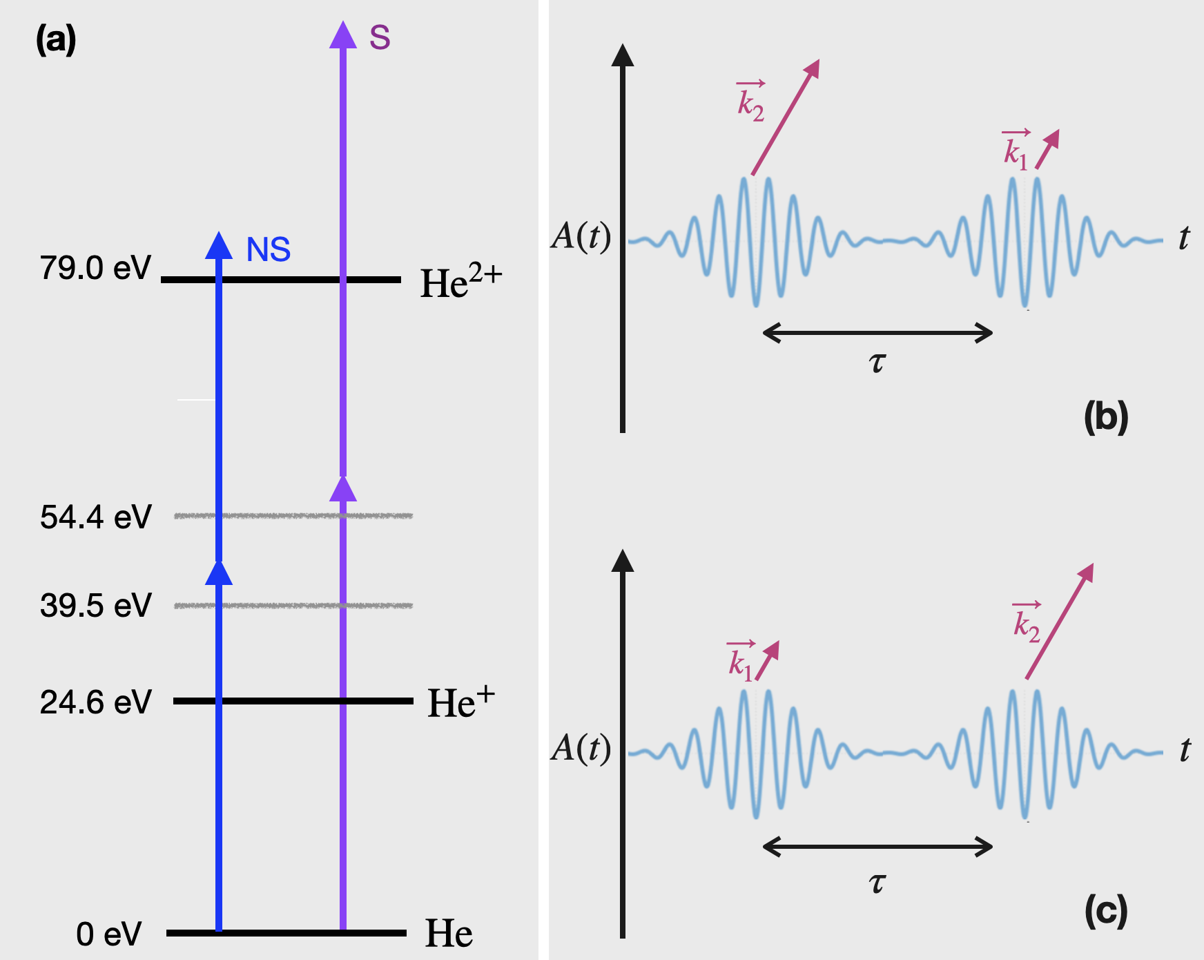
Figure 1: XUV-pump XUV-probe scheme for Helium. (a) Non-sequential (NS) and sequential (S) two-photon double ionization. For two identical XUV photons with energy 39.5 eV $<\omega<$ 54.4 eV, double ionization occurs only through the non-sequential mechanism. At energies well above the sequential threshold, $\omega>$ 54.4 eV, on the other hand, the sequential mechanism dominates. For finite pulses, two different ionization paths (b,c) lead to a same final state, thus giving rise to characteristic interference fringes in the photoelectron coincidence spectrum.

The single-ionization amplitudes of helium are computed using the NewStock atomic ionization code Carette et al. (2013). We describe the ionization channels through a CC expansion containing the three ionic states: $\mathrm{He}^{+}(1s)$, $\mathrm{He}^{+}(2s)$ and $\mathrm{He}^{+}(2p)$ coupled to an additional electron with an associated s, p or d wave to construct augmented channels with total symmetry ${}^{1}S^{e}$ and ${}^{1}P^{o}$. In addition, to improve the short-range description of the electronic correlation, we included a set of localized two-electron wave functions computed with a Multi-Configuration Hartree-Fock calculation (MCHF) performed using the ATSP2K package Froese Fischer et al. (2007). Both the localized and the continuum channels are expanded in terms of the B-spline basis Bachau et al. (2001). We use a simulation box of 300 a.u. ​with $\Delta_{r}=0.4$ a.u. ​node separation to build the B-splines functions of degree 7. With the basis depicted above we obtained a helium ground-state energy $E_{gs}=-2.8846$ a.u., which differs by $\approx 0.02$ a.u. from the NIST energy Kramida et al. (2021). In the figures shown in the rest of the paper, we will shift the photon energies so that the position of the ionization thresholds with respect to the ground state coincide with the experimental ones.

The scattering states corresponding to the single-ionization channels, $|\Psi_{\alpha\vec{k}^{\prime}}^{-}\rangle$ are obtained by solving the Lippmann-Schwinger equation with incoming boundary condition Newton (2014). To test the quality of the intermediate scattering channels defined for the TPDI study, we compare the one-photon total photoionization cross-section with an independent ECS calculation McCurdy and Martín (2004). Fig. 2 compares our results in the length gauge with the benchmark and provides the NewStock velocity gauge as well. The agreement is excellent, with only a few meV difference in the autoionizing state’s position.

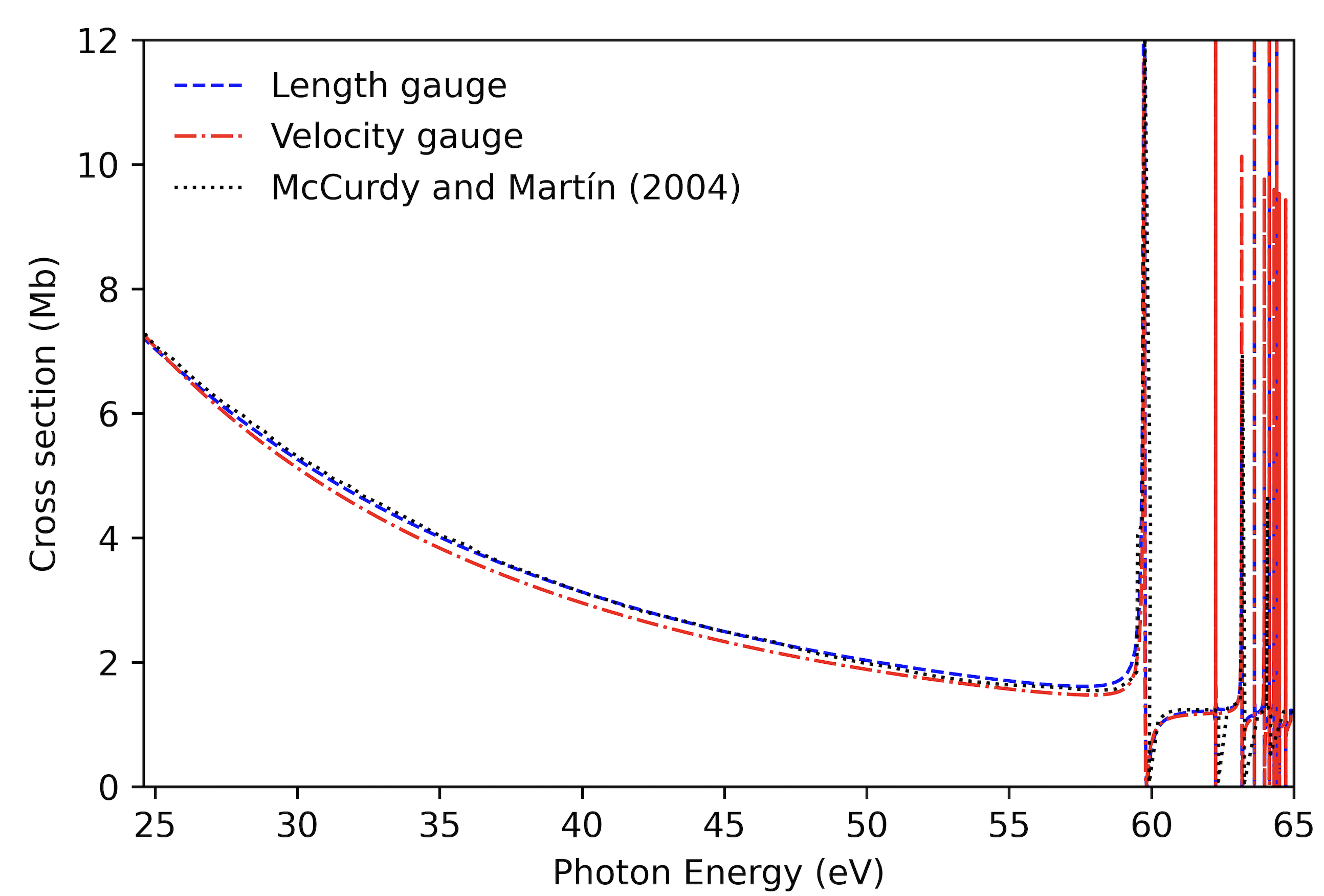
Figure 2: One-photon total photoionization cross-section from the helium ground state computed with NewStock in length (blue dashed line) and velocity gauge (red dashed-dotted line). Results from McCurdy and Martín McCurdy and Martín (2004) (black dotted line) are obtained using the exterior-complex-scaling technique.

The photoionization amplitudes for $\mathrm{He}^{+}$ are computed with a dedicated numerical one-electron code, which also uses B-splines to represent the radial part of the bound and continuum wavefunctions. We use a B-spline basis defined in a uniform grid with degree 7 and node spacing of 0.4 a.u. with a box size of 300 a.u. With these choices, the one-electron code is able to reproduce the analytical results for the bound-bound and bound-continuum dipolar transition amplitudes to machine precision.

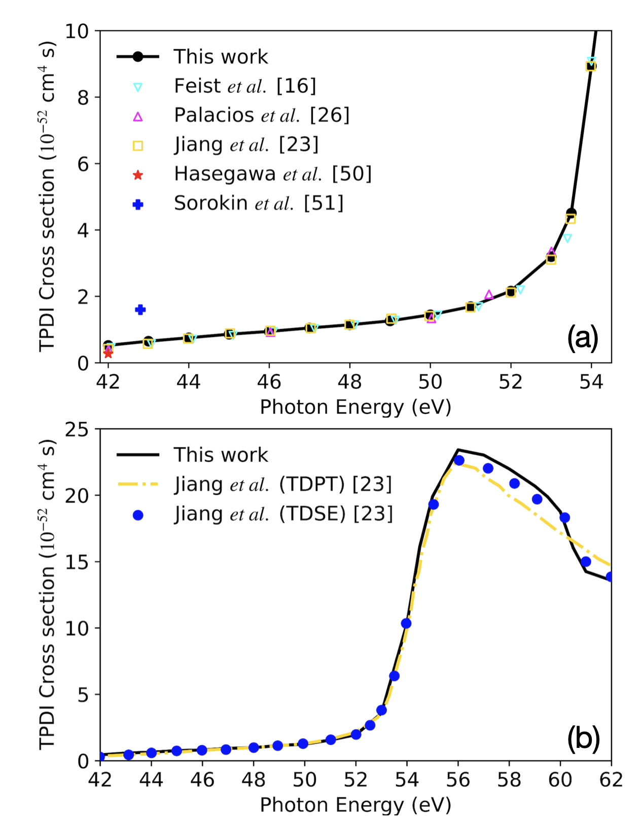
Figure 3: Two-photon double-ionization total cross-section from the helium ground state. (a) Our model results (black circles) with a pulse of duration 20 fs and intensity $4\times 10^{12}$ W/cm² are compared with previous works. (b) Model results with a pulse duration 4 fs and intensity $4\times 10^{12}$ W/cm² compared with the results of TDSE and TDPT models of Ref. Jiang et al. (2015). See text for details.

Figure 3 (a) compares several accurate predictions of the TPDI cross section of helium below the sequential threshold, computed by numerically integrating the TDSE using finite-duration pulses with the analytical predictions of the present FPVSM and with the analytical model from Jiang et al. (2015). To compute the TPDI cross-section, we use Eq. (13) from Ref. Feist et al. (2008), which estimates the TPDI by integrating the total probability over the two photoelectron energies and dividing the result by a form factor proportional to the time integral of the fourth power of the external field. Panel (a) shows our model results with a pulse duration of  20 fs and intensity of $4\cdot 10^{10}$ W/cm². Along with the theoretical results Feist et al. (2008); Palacios et al. (2010); Jiang et al. (2015) previous experimental results Hasegawa et al. (2005); Sorokin et al. (2007) are also shown, which can only confirm the cross section order of magnitude far from the sequential threshold. The cross-section in Ref.  Feist et al. (2008) (down triangles, cyan online) is obtained by solving TDSE with a pulse of duration 4 fs and intensity $10^{12}$ W/cm². Ref. Palacios et al. (2010) (up triangle, magenta online) reports the total TPDI cross-section computed by solving TDSE with a pulse duration of 3 fs. The TDSE calculation from Ref. Jiang et al. (2015) reported in Panel (a) (box, yellow online) corresponds to a pulse duration of 11 fs. The agreement of the model with the numerical simulation is impressive and confirms similar findings based on the virtual sequential model in stationary regime. In particular, the model reproduces the rapid increase in the cross section as the photon energy approaches the sequential threshold already evidenced in Jiang et al. (2015). This rapid increase is due to the enhanced role of the virtual intermediate states when they are close to the resonance condition.

Figure 3 (b) compares the TPDI cross section across the sequential threshold with the original TDSE ab initio calculations and the analytical model from Jiang et al. (2015) with duration 4 fs and intensity of $4\times 10^{12}$ W/cm² with different central photon energies. Notice that while the TDPT model from Jiang et al. (2015) coincides with ours below the sequential threshold, above the sequential threshold, only our model reproduces the resonance profile due to the excitation of the $sp_{2}^{+}$ state, and is in much better agreement with the result from the TDSE simulation.

In our calculations we use pulses with Gaussian profile, whereas the TDSE simulations in Fig. 3 and the analytical model in Jiang et al. (2015) use $\sin^{2}$ envelopes. As long as the width at half maximum of the two field envelope coincide, we do not discern appreciable differences due to the pulse shape. Furthermore, our model can use a linear combination of an arbitrary number of Gaussian pulses, and hence it can reproduce any pulse shape with any desired precision. For example, a linear combination of as few as five Gaussian functions can fit a $\sin^{2}$ profile with an error within 0.001 of the field peak value. Since a single Gaussian function already gives results in line with those with a $\sin^{2}$ profile, however, a calculation with such tailored pulse was not necessary.

III.1 TPDI joint energy distribution with single pulses

This section presents the predictions of the FPVSM in the non-sequential regime as well as across the sequential threshold. To illustrate the transition from the non-sequential threshold, at $\omega=39.5$ eV, to the sequential threshold, at $\omega=54.4$ eV, we look at the joint energy distribution of the two photoelectrons obtained using 500 as XUV Gaussian pulses with peak intensity of $4\cdot 10^{10}$ W/cm² and variable carrier frequency $\omega_{0}$.

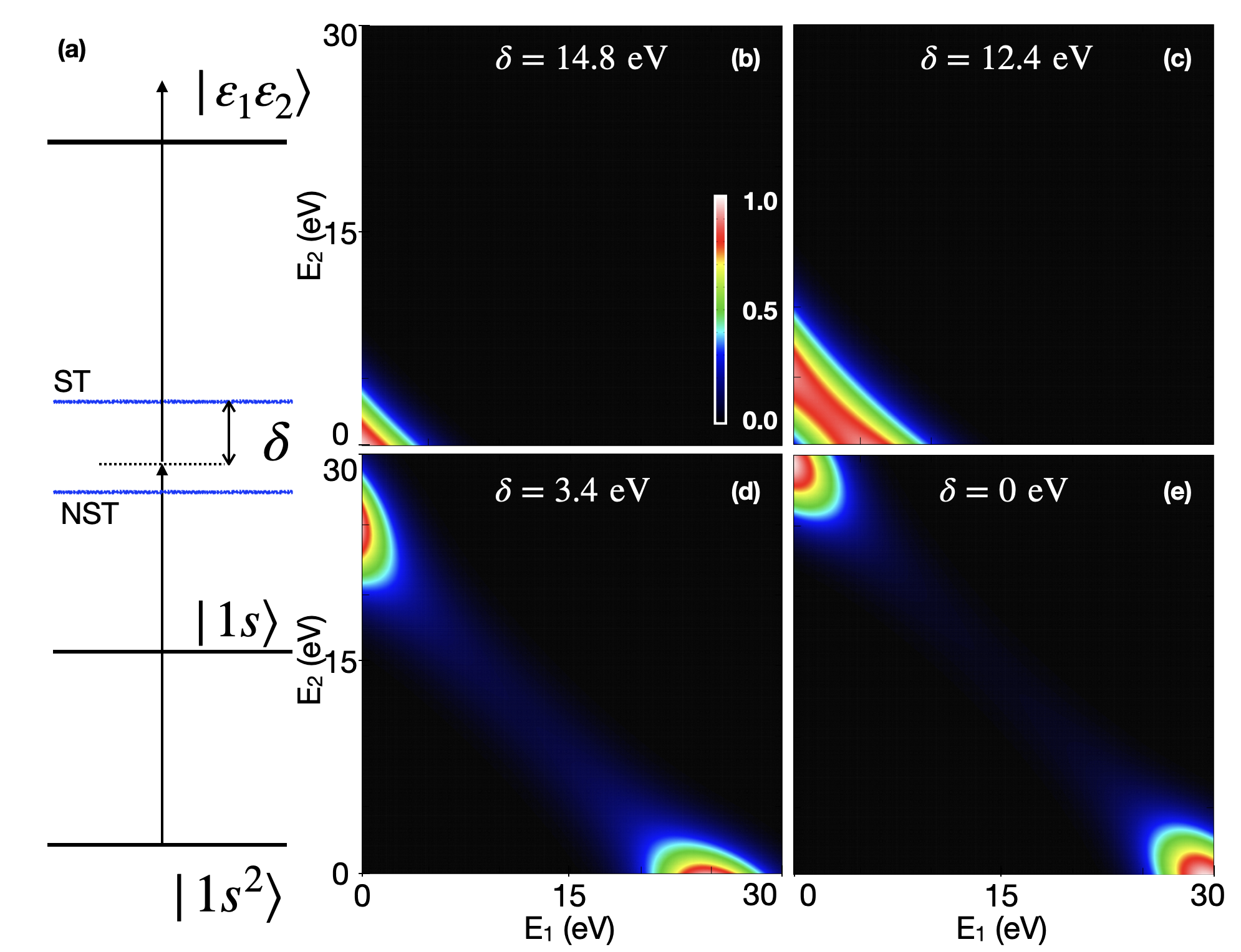
Figure 4: (a) TPDI scheme in the non-sequential regime. $\delta$ is the energy difference from the sequential threshold (ST). Joint energy distribution of two photoelectrons in the non-sequential regime with a fixed pulse duration of 500 as and intensity of $4\cdot 10^{10}$ W/cm² for different central photon energies: (b) 39.5 eV, (c) 42 eV, (d) 51 eV, and (e) 54.4 eV. The joint energy distributions are normalized by a same factor. In the conditions of the present calculation, a peak signal of $1$ corresponds to a TPDI cross section of $6\times 10^{-54}$ cm${}^{4}\,\cdot\,$s$\,\cdot\,$eV^-2

.

Figure 4 (a) shows the TPDI scheme used in the present calculation where $\delta$ is the energy difference from the sequential threshold. Fig. 4 (b) with $\delta$ = 14.8 eV shows the signal appears at the opening threshold of 39.5 eV. As we increase the central photon energy to 42 eV, with $\delta$ = 12.4 eV [Fig. 4 (c)], the strongly correlated joint energy distribution becomes prominently visible. As shown in Fig. 4 (d), as we increase the central photon energy to 51 eV, a two-peak structure emerges, which is the hallmark of the sequential mechanism. At the sequential threshold of 54.4 eV the joint energy distribution shows the two photoelectrons emitted sequentially with energies of 30 eV, respectively.

To disentangle the contribution from different intermediate ionic states, an independent calculation is performed for each CC channel. Fig. 5 (a-d) show the joint energy distribution for each of the intermediate states, $\mathrm{1s}\varepsilon\mathrm{p}$, $\mathrm{2s}\varepsilon\mathrm{p}$, $\mathrm{2p}\varepsilon\mathrm{s}$, and $2p\varepsilon\mathrm{d}$, respectively. With the central photon energy close to the sequential threshold but still well below the $N=2$ shakeup threshold, virtually all the contribution comes from the dominant $\mathrm{1s}\varepsilon\mathrm{p}$ intermediate state.

Figure 5 shows the contribution of individual intermediate channels to the joint energy distribution at $\omega=54$ eV, close to the sequential threshold. At this energy, the distribution resembles that of the sequential mechanism and is dominated by the $1s\epsilon_{p}$ intermediate channel. At this energy, the $2\ell\epsilon_{\ell^{\prime}}$ shakeup channels are still closed and hence they contribute only as virtual excitations, which explains the broad distribution of their energy sharing. Indeed, for closed channels, the pole in the denominator of (7) does not play any fundamental role, thus leading to a continuum distribution for the energy of the first photoelectron.

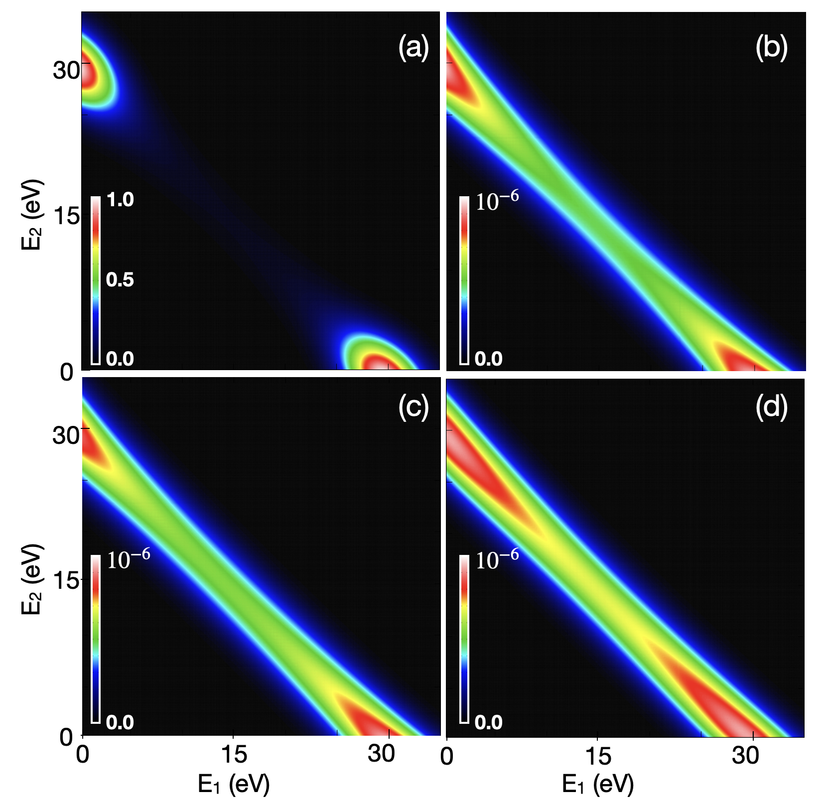
Figure 5: Channel-specific contributions to the photoelectron joint energy distribution for TPDI processes promoted by a 500 as $4\cdot 10^{10}$ W/cm²pulse with central energy of 54 eV: (a) $\mathrm{1s}\varepsilon\mathrm{p}$; (b) $\mathrm{2p}\varepsilon\mathrm{s}$; (c) $\mathrm{2p}\varepsilon\mathrm{d}$; (d) $\mathrm{2s}\varepsilon\mathrm{p}$. The contribution from the $\mathrm{1s}\varepsilon\mathrm{p}$ intermediate channel dominates. The joint energy distributions are normalized by a same factor. In the conditions of the present calculation, a peak signal of $1$ corresponds to a TPDI cross section of $9\times 10^{-52}$ cm${}^{4}\,\cdot\,$s$\,\cdot\,$eV^-2

For ultrashort pulses with central energy above the sequential threshold, the sequential and non-sequential regimes can no longer be separated Feist et al. (2009). Figure 6 (a,b) shows the predictions of the FPVSM for a pulse with central energy of 70 eV and duration of either 120 as (a) or 720 as (b). These plots qualitatively reproduce the results obtained for similar pulses in Feist et al. (2009). In the case of the shorter pulse, in Fig. 6 (a), the parent ion does not have the time to relax and hence the joint energy distribution shows a single peak with a strongly correlated distribution. When the longer pulse is employed, on the other hand, the two-peak structure characteristic of the dominant sequential mechanism clearly emerges. Notice that, in the case of the pulse with short duration, the joint energy distribution exhibits also several sharp features. These features are the imprint of the autoionizing states close to the N=2 threshold, which should not be observed and indeed are not reproduced in fully ab initio simulations. As commented in Sec. II, the presence of resonant profiles is inherent to the FPVSM, since the ion product of an autoionizing state decay is assumed to be immediately available for ionization. This assumption, however, is obviously not satisfied when the duration of the ionizing pulse is much shorter than the lifetime of the autoionizing states in question, which is the case here. For pulses with duration much longer than an autoionizing state lifetime, on the other hand, the model does capture the contribution of the autoionizing state to the two-photon double ionization due to the resonant enhancement (or suppression) of the bound-continuum ionization amplitude, as discussed in the next subsection.

Figure 6: Photoelectron joint energy distribution for TPDI processes promoted by pulses with central energy of 70 eV, peak intensity of $4\cdot 10^{10}$ W/cm² and duration of 120 as (a) and 720 as (b). The joint energy distributions are normalized by a same factor. In the conditions of the present calculation, a peak signal of $1$ corresponds to a TPDI cross section of $0.5\times 10^{-52}$ cm${}^{4}\,\cdot\,$s$\,\cdot\,$eV^-2

Figure 7 shows the photoelectron-pair distribution as a function of the energy sharing $\alpha=E_{1}/(E_{1}+E_{2})$, generated by 500 as pulses with central energy $\omega_{0}$ ranging from 45 eV to 70 eV and with peak intensity of $4\cdot 10^{10}$W/cm². In each case, the distribution is evaluated at the nominal peak of the total energy, $E_{1}+E_{2}=2\omega_{0}-IP$, where $IP$ is the double-ionization potential. In the non-sequential regime, the distribution is almost flat. For energies above the sequential threshold, close to the shake-up threshold, the resonant structure of the autoionizing states emerge. The sharp peak visible for $\omega_{0}=58$ eV corresponds to the $sp_{2}^{+}$ DES. As mentioned earlier, for short pulses, such resonant features are artifacts of the FPVSM. As we approach the double-ionization threshold, the sequential two-peak structure with total energy of 61 eV dominates.

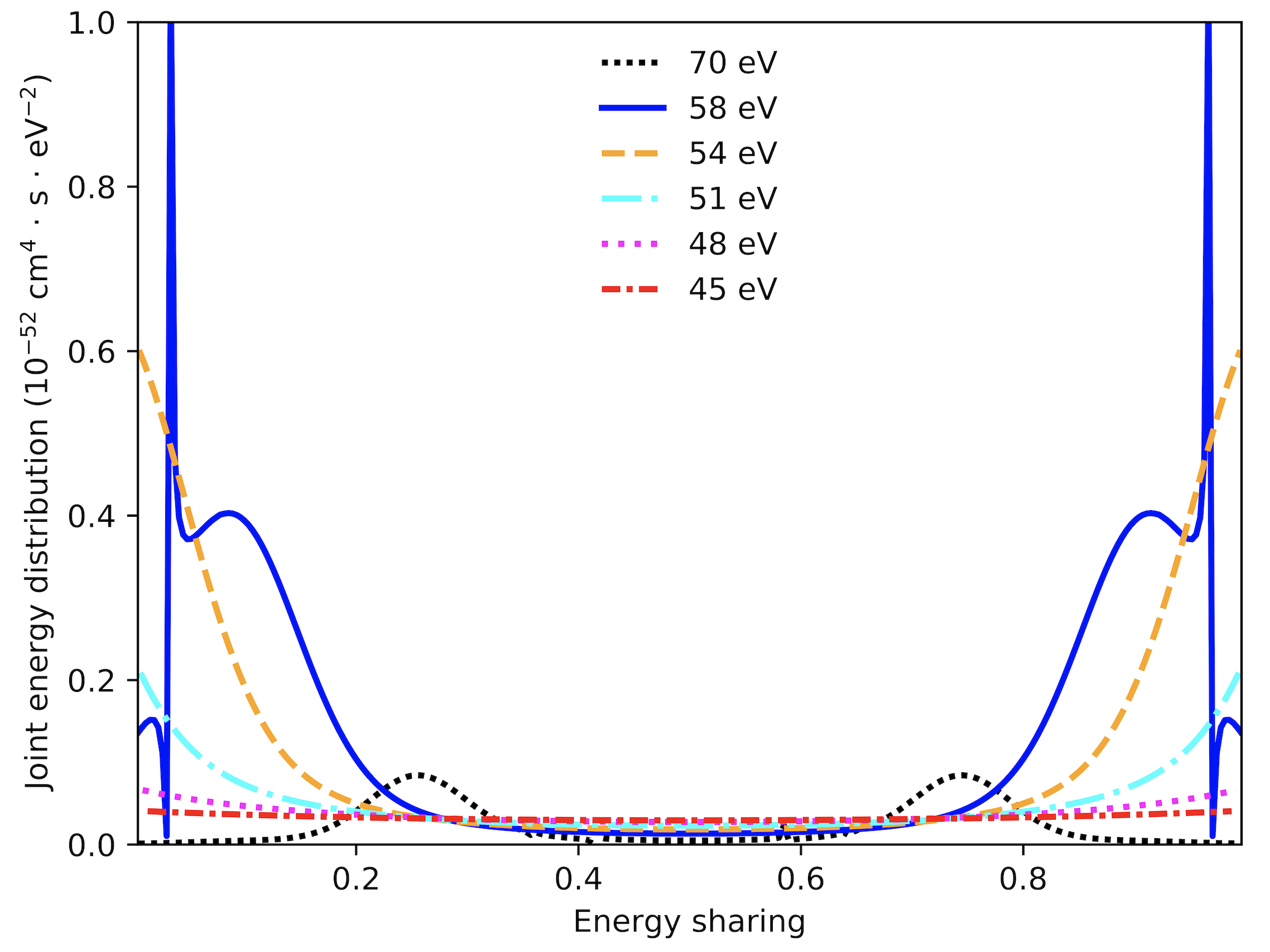
Figure 7: Joint energy distribution as a function of the photoelectron energy sharing, at different photon energies, from the non-sequential up to the sequential regime. The joint energy distributions are normalized by a same factor so that the peak signal correspond to $1.0\times 10^{-52}$ cm${}^{4}\,\cdot\,$s$\,\cdot\,$eV^-2

.

III.2 Pump-probe TPDI

Two-particle quantum interference can be used to probe the entanglement between two identical particles Horne et al. (1989). In the context of photoionization studies, McCurdy and collaborators have shown the two-particle interference in the joint energy distribution of the TPDI process in helium Palacios et al. (2009, 2010). For the present case, we consider a pump-probe scheme of the TPDI of helium with two XUV pulses with a controllable delay $\tau$,

$$\vec{\mathcal{E}}(t)=\vec{\mathcal{E}}_{\textsc{XUV}_{1}}(t)+\vec{\mathcal{E}}_{\textsc{XUV}_{2}}(t-\tau),$$ (12)

where $\vec{\mathcal{E}}_{\textsc{XUV}_{1/2}}(t)$ indicate the transverse electric fields of the two pulses. In the present calculation, the two pulses have central energies $\omega_{1}=30$ eV and $\omega_{2}=60$ eV and duration of 1 fs. At negative time delays, when the 60 eV XUV pulse comes first, the 30 eV XUV pulse is unable to ionize the residual $\mathrm{He}^{+}(1s)$ ion, which has ionization potential 54.4 eV, leading to no TPDI signal around $E_{1}+E_{2}\simeq 11$ eV. If the more energetic pulse exceeded the $2s/2p$ shake-up threshold, one could have observed a signal, since the ionization potential of the excited $\mathrm{He}^{+}$ ion is below 30 eV. At positive time delays, the 30 eV pump pulse ionizes the neutral helium atom and, at some later time $\tau$, the probe pulse ionizes the $\mathrm{He}^{+}$ ion leading to $\mathrm{He}^{2+}$ and two photoelectrons with energies $E_{1}$ and $E_{2}$, as illustrated in Fig. 8 (a).

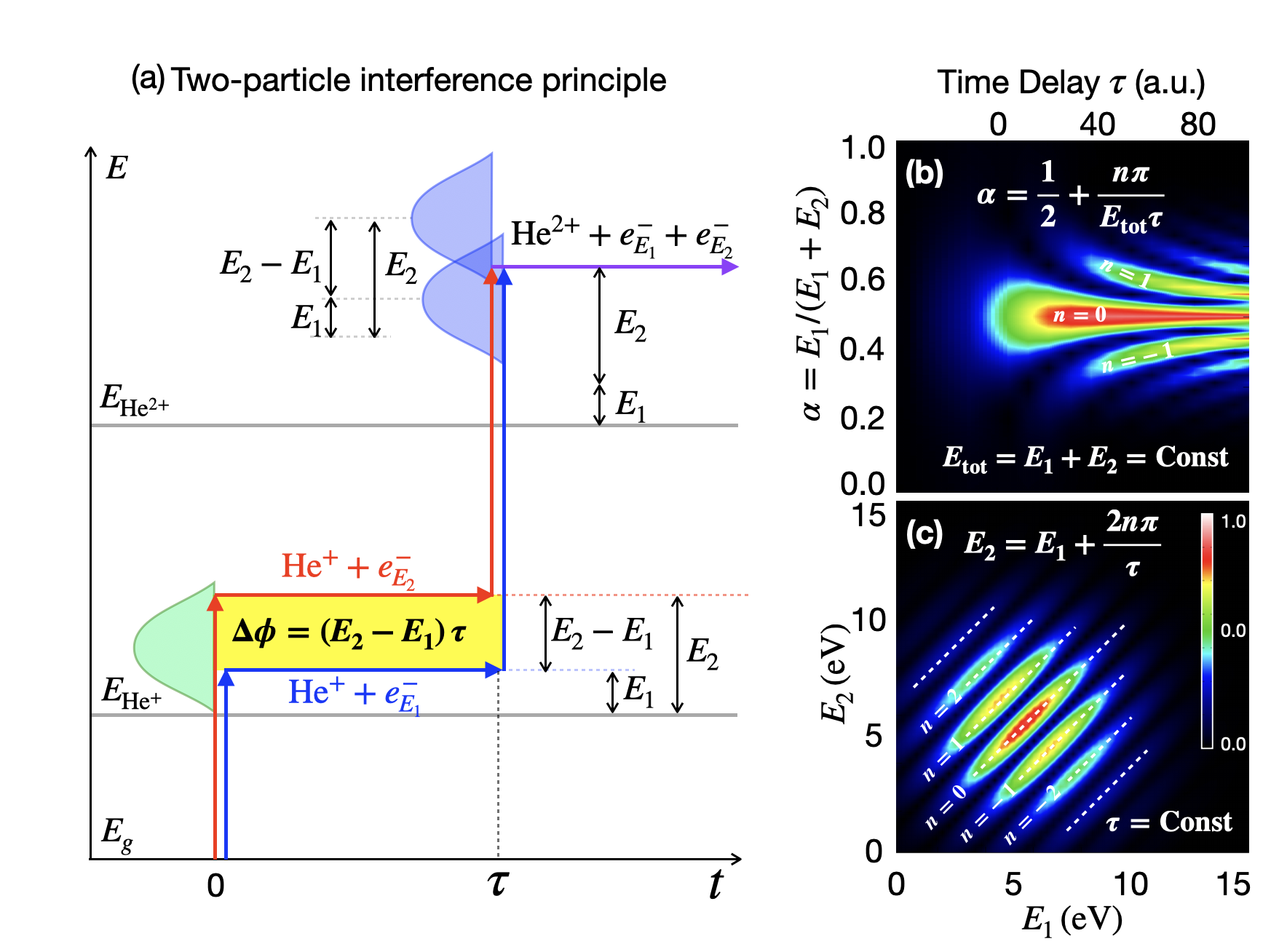
Figure 8: (a) Two-electron quantum interferometric scheme: At time $t$=0, a first XUV photon ionizes the neutral helium atom. After a delay $\tau$, a second XUV photon ionizes $\mathrm{He}^{+}$, creating the $\mathrm{He}^{2+}$ ion and two photoelectrons with energies E₁ and E₂. Two alternative paths (red and blue, online) contribute to this process, leading to interference fringes in the joint energy distribution. (b) joint energy distribution as a function of the photoelectron energy sharing and the pump-probe delay. (c) joint energy distribution as a function of two photoelectron energies for a specific time-delay, $\tau=2$ fs.

Thanks to the finite spectral width of the two pulses, the final state can be reached through two distinct paths. In one path (blue arrows in the figure), the first ionization event generates a photoelectron with energy $E_{1}$ through the absorption of a photon on the lower-frequency edge of the pump-pulse spectrum, whereas in the second ionization event the ion absorbs a photon with frequency on the upper end of the probe-pulse spectrum. In the other path (red arrows in the figure), the order with which the two photoelectrons are generated is reversed. In the interval between the two pulses, the energy of the system along the two path differ by $\Delta E=E_{2}-E_{1}$, and hence the two paths acquire a phase difference $\Delta\phi=(E_{2}-E_{1})\tau$. Since the final state is the same for the two paths, the associated amplitudes interfere constructively or destructively if $\Delta\phi$ is an even or odd integer multiple of $\pi$, respectively. From the energetic point of view, this interference scheme is analogous to the Ramsey interference observed in attosecond pump-probe single-ionization processes Mauritsson et al. (2010); Argenti and Lindroth (2010), where the first step excites the system to different bound metastable states. Here, both events eject a particle and the interference occurs because the two particles being ejected are identical. Constructive interference is realized for $\Delta\phi=2n\pi$,

$$E_{2}=E_{1}+\frac{2\,n\,\pi}{\tau},\qquad n\in\mathbb{Z}.$$ (13)

In the photoelectron joint energy distribution, therefore, the interference fringes appear as straight lines parallel to the $E_{2}=E_{1}$ diagonal, and separated by a distance $d=\sqrt{2}\pi/\tau$ as shown in Fig. 8 (c), as it was already highlighted in Palacios et al. (2009, 2010). Interference fringes are visible also in the energy-sharing spectrum, at a fixed total photoelectron energy $E_{\textrm{tot}}=E_{1}+E_{2}$, as a function of the delay, in which case the condition for constructive interference becomes

$$\alpha=\frac{1}{2}+\frac{n\,\pi}{E_{\mathrm{tot}}\,\tau},\qquad n\in\mathbb{Z}.$$ (14)

In this case, therefore, the fringes have hyperbolic profiles, as shown in Fig. 8 (b), reminescent of those observed in single-ionization attosecond photoelectron spectra Mauritsson et al. (2010). As the time delay between the pulses increases, of course, the interference fringes become difficult to resolve experimentally, and the total signal converges to the incoherent sum of those for the two alternative paths.

As a final example, we examine the FPVSM predictions for the resonant TPDI of helium enhanced by an intermediate DES, using a two-color XUV pump-probe scheme with duration longer than the lifetime of the DES. In all the cases considered in the following, the two pulses have zero relative delay.

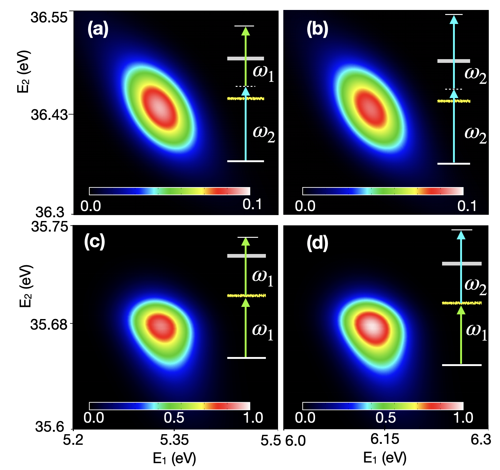
Figure 9: Two-color TPDI: joint energy distribution, as a function of two photoelectron energies, generated by the absorption of two XUV photon from 40 fs pulses with central energies $\omega_{1}=$ 60.15 eV and $\omega_{2}=$ 60.9 eV, and zero relative delay. The lower frequency, $\omega_{1}$, is in resonance with the $\mathrm{sp_{2}^{+}}$ bright doubly-excited state, which is 5.04 eV below the N = 2 threshold and has a lifetime of 17.6 fs. In each panel, the pathway corresponding to the associated signal is shown. The joint energy distributions are normalized by a same factor. In the conditions of the present calculation, a peak signal of $1$ corresponds to a TPDI cross section of $1.5\times 10^{-51}$ cm${}^{4}\,\cdot\,$s$\,\cdot\,$eV^-2.

In the past, the role of DES in TPDI of $\mathrm{He}$ has been studied by solving the TDSE with ultrashort pulses Feist et al. (2011). So far, however, TDSE-based approaches have considered only intense XUV pulses with attosecond or few femtosecond duration, which are difficult to realize experimentally. Here we probe these resonances with longer pulses, which are more easily produced at XFELs facilities. As a case study, we select the $\mathrm{sp_{2}^{+}}$ DES intermediate state, which has a lifetime of 17.6 fs Rost et al. (1997). We study the effect of this state on the joint photoelectron energy distribution in the TPDI of helium with a pair of XUV pulses, each with 40 fs duration and intensity $I=10^{10}\,\mathrm{W/cm^{2}}$.

Figure 9 shows the joint energy distribution when the two pulses have central energy of 60.15 eV and 60.90 eV. The first pulse is resonant with the $1s^{2}-sp_{2}^{+}$ transition, $E_{sp_{2}^{+}}-E_{g}=60.15$ eV. The distribution exhibits four distinct peaks in the $E_{2}>E_{1}$ portion of the spectrum, corresponding to whether both photons are provided from the first pulse [Fig. 9 (c)], from the second pulse [Fig. 9 (b)], or one from each pulse [Fig. 9 (a,d)]. These signals correspond to two resonant (c,d) and two non-resonant (a,b) transitions. Since the peaks are narrow compared with their energy distance in the 2D spectrum, we show them magnified in four separate panels for clarity. The peaks for the non-resonant transitions are symmetric relative to the equal total energy axis, as observed already in the previous section, with ultrashort pulses. Remarkably, the energy distribution is not symmetric anymore in the two resonant cases, which is to be expected given the strong modulation of the first resonant one-photon transition amplitude. In the FPVSM, the resonant modulation of the signal follows the Fano profile of the resonance. Indeed, according to (9), the total ionization amplitude is a linear combination of products of dipole transition amplitudes. With well-separated signals in the joint spectrum, one of these products dominates, owing to the field factor. In the resonant case, therefore, the amplitude factorises into the product of a structureless field form factor times a structureless hydrogenic ionization amplitude of the residual ion and a resonant ionization amplitude from the ground state to the two-electron continuum.

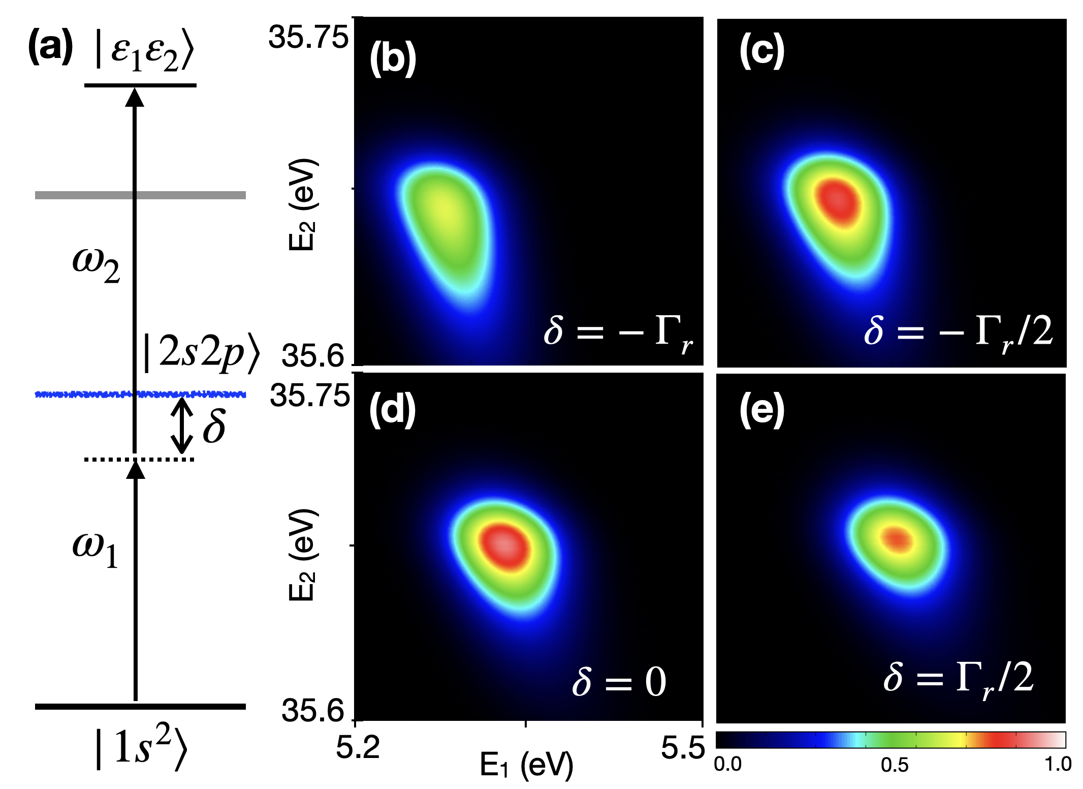
Figure 10: (a) Schematic of the resonant TPDI process, which strongly depends on the detuning $\delta$. (b-e) Joint energy distribution for four different calculations of the resonant TPDI process with fixed $\omega_{2}=60.9$ eV and variable $\omega_{1}=E_{sp_{2}^{+}}-E_{g}+\delta$, where the detuning is indicated in the panels in units of the resonance width $\Gamma_{r}=0.037$ eV. Both pulses have a duration of 40 fs, intensity of $10^{10}$W/cm², and zero relative delay. The joint energy distributions are normalized by a same factor. In the conditions of the present calculation, a peak signal of $1$ corresponds to a TPDI cross section of $1.5\times 10^{-51}$ cm${}^{4}\,\cdot\,$s$\,\cdot\,$eV^-2.

Figure 10 (b-e) show the resonant peak for the transition  10 (a), for four different values of the detuning $\delta$ of the pump-pulse central energy from the $sp_{2}^{+}$ resonance. The probe photon has a fixed central frequency $\omega_{2}=60.9$ eV. The $sp_{2}^{+}$ has a Fano profile with a negative $q$ parameter, i.e., the transition amplitude increases monotonically with energy, peaks, and drops to zero at an energy above the resonant peak, before slowly returning to the background value. This is reflected in the shape of the profile in the four panels: at negative detuning, the signal is stretched below the resonant peak (tail, panel b, c). At positive detuning, the peak and adjacent zero are illuminated, leading to a signal with energy breath considerably narrower than the pump pulse’s and comparable to the resonant width. Even if the resonant profiles of these results are predictable, they are a valuable starting point to assess the deviation of the signal, in the exact resonant double ionization case, due to the partial decay of a resonance, or the contribution of its direct double ionization by the probe pulse, for helium as well as for more complex atoms.

IV Conclusion

In this work, we introduced a finite pulse version of the virtual sequential model (FPVSM), based on ab initio multi-channel one-photon transition amplitudes, to describe the two-photon double ionization process in polyelectronic atoms and, as a proof of principle, we used it to reproduce several features of results for the TPDI of atomic helium, obtained with TDSE simulations. We have calculated the joint energy distribution of the two photoelectrons and the energy sharing from the non-sequential to the sequential regime. The FPVSM allows us to compute the strongly correlated photoelectron joint energy distribution in the non-sequential regime, and the uncorrelated counterpart in the sequential regime, more efficiently than a full TDSE simulation. Unlike previous TDSE simulations, the CC approach in FPVSM allows us to quantify the contribution from different channels and highlights the features associated with each intermediate state under consideration. Furthermore, the model captures how the transition from the non-sequential to sequential blurs as one considers extreme ultrashort pulses with energies near the double ionization threshold. We demonstrate that the energy sharing between the photoelectrons significantly changes as we approach the double ionization threshold and how the two-peak structure emerges in the sequential regime. The model is capable of reproducing the salient features of two-particle interference, already observed in TDSE simulations, which highlight its explanatory power. We have also applied the model to study the asymmetry of the resonant TPDI photoelectron joint energy distribution close to the optically allowed $\mathrm{sp_{2}^{+}}$ doubly-excited state with long XUV-pulses, which is a regime not explored by TDSE simulations. The model admits a natural extension to polyelectronic atoms, which present the additional interesting feature of multiple grand-parent ions. An application of this model to complex atoms such as neon and argon is ongoing and will be subject of future work.

Appendix A Two-photon double ionization matrix element

This appendix details the derivation of the TPDI matrix element (9). Grandparent-ion wavefunctions ($N-2$ electrons) are denoted by the symbol $\Phi_{A}$, and parent-ion wavefunctions ($N-1$ electrons) by the symbol $\Phi_{a}$. The $N-$electron states we will consider here are either bound, $|\Psi_{n}\rangle$, single-ionization, or double ionization states. In the calculation of the $\langle A\,\vec{k}_{1}\sigma_{1}\vec{k}_{2}\sigma_{2}|\mathcal{O}_{\nu}|\Psi_{\alpha\vec{k}^{\prime}}^{-}\rangle$, the single-ionization wave-functions are approximated using the single-channel functions,

$$\Psi^{-}_{\alpha\vec{k}^{\prime}}\simeq\sqrt{N}\hat{\mathcal{A}}_{N}\,\Xi_{\alpha}^{\Gamma}(x_{1}\textrm{\,---\,}x_{N-1};\hat{r}_{N},\zeta_{N})\,\phi_{\alpha,\ell_{\alpha}\epsilon}^{\Gamma\,-}(r_{N})$$ (15)

where in $\Xi_{\alpha}^{\Gamma}(x_{1}\textrm{\,---\,}x_{N-1};\hat{r}_{N},\zeta_{N})$ the parent ion is coupled to the angular and spin part of the $N$-th electron to give rise to a well-defined angular momentum and spin, which are specified in the collective total-symmetry index $\Gamma=(S,L,\Pi;\Sigma,M)$,

$$\Xi_{\alpha}^{\Gamma}(x_{1}\textrm{\,---\,}x_{N-1};\hat{r}_{N},\zeta_{N})=$$

$$=[[\Phi_{a_{\alpha}}(x_{1}\textrm{\,---\,}x_{N-1})\otimes Y_{\ell_{\alpha}}(\hat{r}_{N})]_{LM}\otimes{{}^{2}\chi(\zeta_{N})}]_{S\Sigma}=$$

$$=\sum_{M_{a}m}\sum_{\Sigma_{a}\sigma}C_{L_{a}M_{a},\ell_{\alpha}m}^{LM}C_{S_{a}\Sigma_{a},\frac{1}{2}\sigma}^{S\Sigma}\times$$

$$\times\Phi_{a_{\alpha},M_{a}\Sigma_{a}}(x_{1}\textrm{\,---\,}x_{N-1})Y_{\ell_{\alpha}m}(\hat{r}_{N}){{}^{2}\chi_{\sigma}(\zeta_{N})}.$$ (16)

In (15), the radial photoelectron wavefunction $\phi_{\alpha,\ell_{\alpha}\epsilon}^{\Gamma\,-}(r)$ is normalized in such a way that its outgoing component is

$$\left[\phi_{\alpha,\ell_{\alpha}\epsilon}^{\Gamma\,-}(r)\right]_{\mathrm{out}}=\frac{1}{\sqrt{2\pi k_{\alpha}}}\frac{e^{i\theta_{\alpha}(r)}}{r},\qquad r\to\infty$$ (17)

with $k_{\alpha}=\sqrt{2\epsilon}$, and $\theta_{\alpha}(r)=k_{\alpha}r+\frac{Z}{k_{\alpha}}\ln 2k_{\alpha}r-\ell\pi/2+\sigma_{\ell_{\alpha}}(k_{\alpha})$ is the Coulomb phase factor. Finally, $\mathcal{A}_{N}$ is the idempotent antisymmetrizer,

$$\mathcal{A}_{N}=\frac{1}{N!}\sum_{\mathcal{P}\in\mathcal{S}_{N}}(-1)^{\mathrm{sgn}\mathcal{P}}\mathcal{P},\qquad\mathcal{A}_{N}^{2}=\mathcal{A}_{N}=\mathcal{A}_{N}^{\dagger}.$$ (18)

To define a double-ionization channel, we need to specify, beyond the total quantum numbers $\Gamma$ = $(S,L,\Pi;\Sigma,M)$, the state of the grandparent ion, $\Phi_{A}(x_{1}\textrm{\,---\,}x_{N-2})$ and the non-energy quantum numbers of the two free electrons, namely, their orbital angular momenta, $\ell_{1}$, and $\ell_{2}$, and the angular coupling scheme. Asymptotically

$$\Psi^{-} \phantom{}{}_{A,E_{1}\ell_{1}m_{1}\sigma_{1},E_{2}\ell_{2}m_{2}\sigma_{2}}=\sqrt{N(N-1)}\hat{\mathcal{A}}_{N}\,\times$$ (19)

$$\times\Psi_{A}(x_{1}\textrm{\,---\,}x_{N-2})\otimes$$

$$\otimes{{}^{2}\phi^{-}_{E_{1}\ell_{1}m_{1}\sigma_{1}}}(x_{N-1})\otimes{{}^{2}\phi^{-}_{E_{2}\ell_{2}m_{2}\sigma_{2}}}(x_{N}).$$

This expression can be cast in a symmetrized combination in which either electron $1$ or $2$ is recoupled with the grand-parent-ion $A$ to give rise to a scattering state for the system with $N-1$ electron. Once the transition amplitudes to the states in (19) are known, the fully differential TPDI amplitude is readily reconstructed using the expansion of energy-normalized Coulomb plane waves,

$$\begin{split}\psi_{E\hat{\Omega}}^{-}(\vec{r})&=\sqrt{\frac{2k}{\pi}}\sum_{\ell m}i^{\ell}e^{-i\sigma_{\ell}}F_{\ell}(kr)Y_{\ell m}^{*}(\hat{k})Y_{\ell m}(\hat{r})\\ &=\sum_{\ell m}i^{\ell-1}e^{-i\sigma_{\ell}}Y_{\ell m}^{*}(\hat{k})\phi^{-}_{\ell mE}(\vec{r}).\end{split}$$ (20)

As the next step in the application of the FPVSM, one of the two photoelectron is angularly and spin and permutationally coupled to the grand-parent ion, using the well-known identities $\delta_{\alpha\alpha^{\prime}}\delta_{\beta\beta^{\prime}}=\sum_{c\gamma}C_{a\alpha,b\beta}^{c\gamma}C_{a\alpha^{\prime},b\beta^{\prime}}^{c\gamma}$ and $\hat{\mathcal{A}}_{N}=\frac{1}{N}[1-(N-1)\mathcal{P}_{N-1,N}]\hat{\mathcal{A}}_{N-1}$. Finally, the recoupled grand-parent/photoelectron state is identified with the scattering state of the singly ionized system that satisfies the same outgoing boundary conditions. Since this identification is in itself an approximation, it breaks the symmetry between the two photoelectrons. To avoid such bias in the result, therefore, it is convenient to symmetrically split (19) first and, in each of the two resulting identical components, couple the grandparent ion to either the first or the second photoelectron. The result of this tedious but straightforward process is

$$\begin{split}\Psi^{-}_{A,E_{1}\ell_{1}m_{1}\sigma_{1},E_{2}\ell_{2}m_{2}\sigma_{2}}&=\frac{1-(N-1)\mathcal{P}_{N-1,N}}{2\sqrt{N}}\sum_{\Gamma_{\aleph}}C_{L_{A}M_{A},\ell_{1}m_{1}}^{L_{\aleph}M_{\aleph}}C_{S_{A}\Sigma_{A},\frac{1}{2}\sigma_{1}}^{S_{\aleph}\Sigma_{\aleph}}\Psi^{-}_{\aleph E_{1}}(x_{1}\textrm{\,---\,}x_{N-1})\otimes{{}^{2}\phi^{-}_{E_{2}\ell_{2}m_{2}\sigma_{2}}}(x_{N})-\\ &-\frac{1-(N-1)\mathcal{P}_{N-1,N}}{2\sqrt{N}}\sum_{\Gamma_{\beth}}C_{L_{A}M_{A},\ell_{2}m_{2}}^{L_{\beth}M_{\beth}}C_{S_{A}\Sigma_{A},\frac{1}{2}\sigma_{2}}^{S_{\beth}\Sigma_{\beth}}\Psi^{-}_{\beth E_{2}}(x_{1}\textrm{\,---\,}x_{N-1})\otimes{{}^{2}\phi^{-}_{E_{1}\ell_{1}m_{1}\sigma_{1}}}(x_{N})\end{split}$$ (21)

where the summations are constrained so that $\ell_{\aleph}=\ell_{1}$, $\ell_{\beth}=\ell_{2}$, and we have introduced

$$\Psi^{-}_{\aleph E_{1}}(x_{1}\textrm{\,---\,}x_{N-1})=\sqrt{N-1}\,\hat{\mathcal{A}}_{N-1}\sum_{M_{A}^{\prime}m_{1}^{\prime}\Sigma_{A}^{\prime}\sigma_{1}^{\prime}}C_{L_{A}M_{A}^{\prime},\ell_{1}m_{1}^{\prime}}^{L_{\aleph}M_{\aleph}}C_{S_{A}\Sigma_{A}^{\prime},\frac{1}{2}\sigma_{1}^{\prime}}^{S_{\aleph}\Sigma_{\aleph}}\Psi_{A,\Sigma_{A}^{\prime},M_{A}^{\prime}}(x_{1}\textrm{\,---\,}x_{N-2})\otimes{{}^{2}\phi^{-}_{E_{1}\ell_{1}m_{1}^{\prime}\sigma_{1}^{\prime}}}(x_{N-1}).$$ (22)

To evaluate the dipole matrix element between a double ionization and a single ionization continuum, we further assume that the unbound electron in the latter does not participate in the transition and plays the role of a spectator instead.

Using Wigner-Eckart theorem and the orthogonality of the continuum wave functions, we get

$$\begin{split}&\langle\Psi^{-}_{A,E_{1}\ell_{1}m_{1}\sigma_{1},E_{2}\ell_{2}m_{2}\sigma_{2}}|\mathcal{O}_{\nu}|\Psi_{\alpha E}^{\Gamma(-)}\rangle=\\ =&\frac{1}{2}\sum_{\Sigma_{\aleph}}C_{S_{A}\Sigma_{A},\frac{1}{2}\sigma_{1}}^{S_{a}\Sigma_{\aleph}}C_{S_{a}\Sigma_{\aleph},\frac{1}{2}\sigma_{2}}^{S\Sigma}\sum_{L_{\aleph}}\frac{1}{\Pi_{L_{\aleph}}}\langle\Psi^{-}_{\aleph E_{1}}\|\mathcal{O}_{1}\|\Phi_{a_{\alpha}}\rangle\,\delta_{\ell_{2}\ell_{\alpha}}\delta(E-E_{a}-E_{2})\sum_{M_{\aleph}M_{a}}C_{L_{A}M_{A},\ell_{1}m_{1}}^{L_{\aleph}M_{\aleph}}C_{L_{a}M_{a},\ell_{2}m_{2}}^{LM}C_{L_{a}M_{a},1\nu}^{L_{\aleph}M_{\aleph}}-\\ -&\frac{1}{2}\sum_{\Sigma_{\beth}}C_{S_{A}\Sigma_{A},\frac{1}{2}\sigma_{2}}^{S_{a}\Sigma_{\beth}}C_{S_{a}\Sigma_{\beth},\frac{1}{2}\sigma_{1}}^{S\Sigma}\sum_{L_{\beth}}\frac{1}{\Pi_{L_{\beth}}}\langle\Psi^{-}_{\beth E_{2}}\|\mathcal{O}_{1}\|\Phi_{a_{\alpha}}\rangle\,\delta_{\ell_{1}\ell_{\alpha}}\delta(E-E_{a}-E_{1})\sum_{M_{\beth}M_{a}}C_{L_{A}M_{A},\ell_{2}m_{2}}^{L_{\beth}M_{\beth}}C_{L_{a}M_{a},\ell_{1}m_{1}}^{LM}C_{L_{a}M_{a},1\nu}^{L_{\beth}M_{\beth}}\end{split}$$ (23)

Now, we can evaluate the two-photon matrix element

$$\begin{split}&\langle\Psi^{-}_{A,E_{1}\ell_{1}m_{1}\sigma_{1},E_{2}\ell_{2}m_{2}\sigma_{2}}|\mathcal{O}_{\nu}G_{0}^{+}(E_{g}+\omega)\mathcal{O}_{\mu}|g\rangle=\sum_{\Gamma\alpha}\int dE\frac{\langle\Psi^{-}_{A,E_{1}\ell_{1}m_{1}\sigma_{1},E_{2}\ell_{2}m_{2}\sigma_{2}}|\mathcal{O}_{\nu}|\Psi_{\alpha E}^{\Gamma(-)}\rangle\,\langle\Psi_{\alpha E}^{\Gamma(-)}|\mathcal{O}_{\mu}|g\rangle}{E_{g}+\omega-E+i0^{+}}\end{split}$$ (24)

In the relevant special case of an initial states with ¹S symmetry,

$$\begin{split}&\langle\Psi^{-}_{A,E_{1}\ell_{1}m_{1}\sigma_{1},E_{2}\ell_{2}m_{2}\sigma_{2}}|\mathcal{O}_{\nu}G_{0}^{+}(E_{g}+\omega)\mathcal{O}_{\mu}|g\rangle=\\ =&\frac{1-\mathcal{P}_{12}}{2\sqrt{3}}\frac{C_{\frac{1}{2}\sigma_{2},\frac{1}{2}\sigma_{1}}^{S_{A}-\Sigma_{A}}}{\Pi_{S_{A}}}\sum_{aL}\frac{1}{\Pi_{L}}\frac{\langle\Psi^{{}^{2S_{a}+1}L^{\bar{\pi}_{a}}(-)}_{A\ell_{1}E_{1}}\|\mathcal{O}_{1}\|\Phi_{a}\rangle\,\langle\Psi_{a\ell_{2}E_{2}}^{{{}^{1}P^{o}}(-)}\|\mathcal{O}_{1}\|g\rangle}{E_{g}+\omega-E_{a}-E_{2}+i0^{+}}\sum_{MM_{a}}C_{L_{A}M_{A},\ell_{1}m_{1}}^{LM}C_{L_{a}M_{a},\ell_{2}m_{2}}^{1\mu}C_{L_{a}M_{a},1\nu}^{LM},\end{split}$$ (25)

where $\bar{e}=o$ and vice versa. Convolution with the external field (6) readily yields (9).

Appendix B Two-photon frequency integral

In this appendix, we derive the general formula for the two-photon frequency integral that appears in Eq. (9) in terms of Faddeyeva function,

$$I_{21}=\int d\omega\frac{\tilde{A}_{2}(E_{n}-\omega)\tilde{A}_{1}(\omega)}{E_{p}+\omega+i0^{+}},$$ (26)

where the numerator frequency detuning $E_{n}$ and the pole shift $E_{p}$ are known functions of the final energy of the two photoelectrons as well as of the energy of the intermediate and final ion, whereas $\tilde{A}_{i}(\omega)$ ($i=1,2$) are the spectra of two unchirped Gaussian pulses. Here, the vector potentials of the two linearly polarized pulses in the time domain (notice that since we are considering arbitrary sequences of linearly polarized pulses, we are also automatically including the case of arbitrarily polarized pulses as well), $\vec{A}_{i}(t)$, are defined as $\vec{A}_{i}(t)=\hat{\epsilon}_{i}A_{i}e^{-\sigma_{i}^{2}(t-t_{i})^{2}/2}\cos\left[(\omega-\omega_{i})t+\varphi_{i}\right]$, where $\hat{\epsilon}_{i}$ is the light polarization, $A_{i}$ is the vector potential amplitude, $\varphi_{i}$ the carrier-envelope phase, $\omega_{i}$ the central frequency, and $\sigma_{i}$ the standard deviation of the vector-potential spectrum. The temporal duration of the pulse, normally identified with the full-width at half maximum (fwhm) of the pulse intensity, is then fwhm$=2\sqrt{\ln 2}\sigma_{i}^{-1}$. In the following it is useful to split each pulse $\vec{A}_{i}(t)$ in its positive- and negative-central-frequency components $\vec{A}^{\pm}_{i}(t)$, $\vec{A}_{i}(t)=\vec{A}^{+}_{i}(t)+\vec{A}^{-}_{i}(t)$, $\vec{A}^{\pm}_{i}(t)=\hat{\epsilon}_{i}\frac{A_{i}}{2}e^{-\sigma_{i}^{2}(t-t_{i})^{2}/2}e^{\pm i\left[(\omega-\omega_{i})t+\varphi_{i}\right]}$. The pulse spectrum, defined as

$$\tilde{A}_{i}(\omega)\equiv(2\pi)^{-1/2}\int dt\,\,\hat{\epsilon}_{i}^{*}\cdot A_{i}(t)e^{i\omega t},$$ (27)

also separates in the sum of a positive- and a negative-central-frequency component, $\tilde{A}_{i}(\omega)=\tilde{A}_{i}^{+}(\omega)+\tilde{A}_{i}^{-}(\omega)$,

$$\begin{split}\tilde{A}_{i}^{\pm}(\omega)&=\frac{A_{i}}{2\sigma_{i}}\exp\left[i(\omega t_{i}\mp\varphi_{i})-(\omega\mp\omega_{i})^{2}/2\sigma_{i}^{2}\right].\end{split}$$ (28)

In the case of the absorption of two photons,

$$I_{21}=\int d\omega\frac{\tilde{A}_{2}^{+}(E_{n}-\omega)\tilde{A}_{1}^{+}(\omega)}{E_{p}+\omega+i0^{+}}.$$ (29)

Let us introduce the delay $\tau$ between the two pulses, $\tau=t_{2}-t_{1}$. The numerator in (29) then reads

$$\tilde{A}_{2}^{+}(E_{n}-\omega)\tilde{A}_{1}^{+}(\omega)=\frac{A_{1}A_{2}}{4\sigma_{1}\sigma_{2}}\,e^{-i(\varphi_{1}+\varphi_{2})}\,e^{iE_{n}t_{2}}\times$$ (30)

$$\times \exp\left[-\frac{(\omega-\omega_{1})^{2}}{2\sigma_{1}^{2}}-\frac{\left(\omega-E_{n}+\omega_{2}\right)^{2}}{2\sigma_{2}^{2}}-i\omega\tau\right]$$

and the frequency integral $I_{21}$ can be rewritten as

$$I_{21} = \frac{A_{1}A_{2}}{4\sigma_{1}\sigma_{2}}\,e^{-i(\varphi_{1}+\varphi_{2}-E_{n}t_{2})}\times$$ (31)

$$\times e^{-\omega_{1}^{2}/2\sigma_{1}^{2}-(E_{n}-\omega_{2})^{2}/2\sigma_{2}^{2}+\sigma_{t}^{2}(\tilde{\omega}-E_{p})^{2}/2}\times$$

$$\times \int_{-\infty}^{\infty}d\omega\,\frac{\exp[-\sigma_{t}^{2}(\omega-\tilde{\omega})^{2}/2]}{\omega+i0^{+}},$$

where we have introduced the new parameters

$$\sigma_{t} = \sqrt{1/\sigma_{1}^{2}+1/\sigma_{2}^{2}},$$ (32)

$$\tilde{\omega} = E_{p}+\left(\frac{\omega_{1}}{\sigma_{1}^{2}}+\frac{E_{n}-\omega_{2}}{\sigma_{2}^{2}}-i\tau\right)/\sigma_{t}^{2}.$$ (33)

The residual integral in (31) can be expressed in closed form in terms of the Faddeyeva function of complex argument, $\mathcal{W}(z)$, which, in the upper complex semi-plane, admits the following integral representation (see  (DLMF, , (7.7.2))),

$$\mathcal{W}(z)\equiv\frac{i}{\pi}\int_{-\infty}^{\infty}\frac{e^{-t^{2}}\,dt}{z-t},\qquad\imaginary z>0.$$ (34)

The Faddeyeva function can be extended analytically to the remainder of the complex plane, $\mathcal{W}(z)=2/e^{z^{2}}-\mathcal{W}(-z)$. To compute the frequency integral, let us change the integration variable from $\omega$ to $y=\sigma_{t}(\omega-\tilde{\omega})/\sqrt{2}$,

$$\int_{-\infty}^{\infty}d\omega\,\frac{\exp[-\sigma_{t}^{2}(\omega-\tilde{\omega})^{2}/2]}{\omega+i0^{+}}=\int_{-\infty+i\,\imaginary z}^{\infty+i\,\imaginary z}\frac{e^{-y^{2}}\,dy}{z-i0^{+}-y},$$

where $z=-\sigma_{t}\tilde{\omega}/\sqrt{2}$.

If $\imaginary z>0$, the pole $z-i0^{+}$ is below the integration path,

$$\int_{-\infty+i\,\imaginary z}^{\infty+i\,\imaginary z} \frac{e^{-y^{2}}\,dy}{z-i0^{+}-y}=\int_{-\infty}^{\infty}\frac{e^{-y^{2}}\,dy}{z-y}-2\,e^{-z^{2}}$$ (35)

$$= -i\pi\mathcal{W}(z)+2i\pi\,e^{-z^{2}}=i\pi\mathcal{W}(-z).$$

The same result is obtained for $\imaginary z<0$, and hence

$$I_{21} = -i\pi\frac{A_{1}A_{2}}{4\sigma_{1}\sigma_{2}}\,e^{-i(\varphi_{1}+\varphi_{2}-E_{n}t_{2})}\,\times$$

$$\times e^{-\omega_{1}^{2}/2\sigma_{1}^{2}-(E_{n}-\omega_{2})^{2}/2\sigma_{2}^{2}+\sigma_{t}^{2}(\tilde{\omega}-E_{p})^{2}/2}\,\,\mathcal{W}\left(\frac{\sigma_{t}\tilde{\omega}}{\sqrt{2}}\right).$$

References

- Corkum and Krausz (2007) P. B. Corkum and F. Krausz, “Attosecond science,” Nat. Phys. 3, 381–387 (2007).
- Krausz and Ivanov (2009) F. Krausz and M. Ivanov, “Attosecond physics,” Rev. Mod. Phys. 81, 163–234 (2009).
- Pazourek et al. (2015) R. Pazourek, S. Nagele, and J. Burgdörfer, “Attosecond chronoscopy of photoemission,” Rev. Mod. Phys. 87, 765–802 (2015).
- Duris et al. (2020) J. Duris, S. Li, T. Driver, E. G. Champenois, J. P. MacArthur, A. A. Lutman, Z. Zhang, P. Rosenberger, J. W. Aldrich, R. Coffee, G. Coslovich, F-J. Decker, J. M. Glownia, G. Hartmann, W. Helml, A. Kamalov, J. Knurr, J. Krzywinski, M-F Lin, J. P. Marangos, M. Nantel, A. Natan, J. T. O’Neal, N. Shivaram, P. Walter, A. L. Wang, J. J. Welch, T. J. A. Wolf, J. Z. Xu, M. F. Kling, P. H. Bucksbaum, A. Zholents, Z. Huang, J. P. Cryan, and A. Marinelli, “Tunable isolated attosecond x-ray pulses with gigawatt peak power from a free-electron laser,” Nature Photonics 14, 30 (2020).
- Saito et al. (2019) Nariyuki Saito, Hiroki Sannohe, Nobuhisa Ishii, Teruto Kanai, Nobuhiro Kosugi, Yi Wu, Andrew Chew, Seunghwoi Han, Zenghu Chang, and Jiro Itatani, “Real-time observation of electronic, vibrational, and rotational dynamics in nitric oxide with attosecond soft x-ray pulses at 400 eV,” Optica 6, 1542–1546 (2019).
- Borrego-Varillas et al. (2022) Rocío Borrego-Varillas, Matteo Lucchini, and Mauro Nisoli, “Attosecond spectroscopy for the investigation of ultrafast dynamics in atomic, molecular and solid-state physics,” Rep. Prog. Phys. 85, 066401 (2022).
- Weber et al. (2000) Th Weber, Harald Giessen, Matthias Weckenbrock, Gunter Urbasch, Andre Staudte, Lutz Spielberger, Ottmar Jagutzki, Volker Mergel, Martin Vollmer, and Reinhard Dörner, “Correlated electron emission in multiphoton double ionization,” Nature 405, 658–661 (2000).
- Bergues et al. (2012) Boris Bergues, Matthias Kübel, Nora G Johnson, Bettina Fischer, Nicolas Camus, Kelsie J Betsch, Oliver Herrwerth, Arne Senftleben, A Max Sayler, Tim Rathje, et al., “Attosecond tracing of correlated electron-emission in non-sequential double ionization,” Nature Commun. 3, 813 (2012).
- Månsson et al. (2014) Erik P Månsson, Diego Guénot, Cord L Arnold, David Kroon, Susan Kasper, J Marcus Dahlström, Eva Lindroth, Anatoli S Kheifets, Anne L’huillier, Stacey L Sorensen, et al., “Double ionization probed on the attosecond timescale,” Nature Physics 10, 207–211 (2014).
- Horner et al. (2007) D. A. Horner, F. Morales, T. N. Rescigno, F. Martín, and C. W. McCurdy, “Two-photon double ionization of helium above and below the threshold for sequential ionization,” Phys. Rev. A 76, 030701 (2007).
- Ivanov and Kheifets (2007) I. A. Ivanov and A. S. Kheifets, “Two-photon double ionization of helium in the region of photon energies eV,” Phys. Rev. A 75, 033411 (2007).
- Horner et al. (2008a) D. A. Horner, C. W. McCurdy, and T. N. Rescigno, “Triple differential cross sections and nuclear recoil in two-photon double ionization of helium,” Phys. Rev. A 78, 043416 (2008a).
- Horner et al. (2008b) D. A. Horner, T. N. Rescigno, and C. W. McCurdy, “Decoding sequential versus nonsequential two-photon double ionization of helium using nuclear recoil,” Phys. Rev. A 77, 030703 (2008b).
- Førre et al. (2010) M. Førre, S. Selstø, and R. Nepstad, “Nonsequential two-photon double ionization of atoms: Identifying the mechanism,” Phys. Rev. Lett. 105, 163001 (2010).
- Nikolopoulos and Lambropoulos (2001) L. A. A. Nikolopoulos and P. Lambropoulos, “Multichannel theory of two-photon single and double ionization of helium,” J. Phys. B: At. Mol. Opt. Phys. 34, 545–564 (2001).
- Feist et al. (2008) J. Feist, S. Nagele, R. Pazourek, E. Persson, B. I. Schneider, L. A. Collins, and J. Burgdörfer, “Nonsequential two-photon double ionization of helium,” Phys. Rev. A 77, 043420 (2008).
- Foumouo et al. (2008) Emmanuel Foumouo, Philippe Antoine, Henri Bachau, and Bernard Piraux, “Attosecond timescale analysis of the dynamics of two-photon double ionization of helium,” New J. Phys. 10, 025017 (2008).
- Palacios et al. (2008) A. Palacios, T. N. Rescigno, and C. W. McCurdy, “Cross sections for short-pulse single and double ionization of helium,” Phys. Rev. A 77, 032716 (2008).
- Nepstad et al. (2010) R. Nepstad, T. Birkeland, and M. Førre, “Numerical study of two-photon ionization of helium using an ab initio numerical framework,” Phys. Rev. A 81, 063402 (2010).
- Guan et al. (2008) Xiaoxu Guan, K. Bartschat, and B. I. Schneider, “Dynamics of two-photon double ionization of helium in short intense XUV laser pulses,” Phys. Rev. A 77, 043421 (2008).
- Hu et al. (2004) S. X. Hu, J. Colgan, and L. A. Collins, “Triple-differential cross-sections for two-photon double ionization of he near threshold,” J. Phys. B: At. Mol. Opt. Phys. 38, L35–L45 (2004).
- Colgan and Pindzola (2002) J. Colgan and M. S. Pindzola, “Core-excited resonance enhancement in the two-photon complete fragmentation of helium,” Phys. Rev. Lett. 88, 173002 (2002).
- Jiang et al. (2015) Wei-Chao Jiang, Jun-Yi Shan, Qihuang Gong, and Liang-You Peng, “Virtual sequential picture for nonsequential two-photon double ionization of helium,” Phys. Rev. Lett. 115, 153002 (2015).
- Palacios et al. (2009) A. Palacios, T. N. Rescigno, and C. W. McCurdy, “Two-electron time-delay interference in atomic double ionization by attosecond pulses,” Phys. Rev. Lett. 103, 253001 (2009).
- Feist et al. (2009) J. Feist, S. Nagele, R. Pazourek, E. Persson, B. I. Schneider, L. A. Collins, and J. Burgdörfer, “Probing electron correlation via attosecond XUV pulses in the two-photon double ionization of helium,” Phys. Rev. Lett. 103, 063002 (2009).
- Palacios et al. (2010) A. Palacios, D. A. Horner, T. N. Rescigno, and C. W. McCurdy, “Two-photon double ionization of the helium atom by ultrashort pulses,” J. Phys. B: At. Mol. Opt. Phys. 43, 194003 (2010).
- Feist et al. (2011) J. Feist, S. Nagele, C. Ticknor, B. I. Schneider, L. A. Collins, and J. Burgdörfer, “Attosecond two-photon interferometry for doubly excited states of helium,” Phys. Rev. Lett. 107, 093005 (2011).
- Pazourek et al. (2011) R. Pazourek, J. Feist, S. Nagele, E. Persson, B. I. Schneider, L. A. Collins, and J. Burgdörfer, “Universal features in sequential and nonsequential two-photon double ionization of helium,” Phys. Rev. A 83, 053418 (2011).
- Bachau (2011) H. Bachau, “Theory of two-photon double ionization of helium at the sequential threshold,” Phys. Rev. A 83, 033403 (2011).
- Zhang et al. (2011) Zheng Zhang, Liang-You Peng, Ming-Hui Xu, Anthony F. Starace, Toru Morishita, and Qihuang Gong, “Two-photon double ionization of helium: Evolution of the joint angular distribution with photon energy and two-electron energy sharing,” Phys. Rev. A 84, 043409 (2011).
- Yu and Madsen (2016) Chuan Yu and Lars Bojer Madsen, “Sequential and nonsequential double ionization of helium by intense xuv laser pulses: Revealing ac stark shifts from joint energy spectra,” Phys. Rev. A 94, 053424 (2016).
- Jiang et al. (2017) Wei-Chao Jiang, Stefan Nagele, and Joachim Burgdörfer, “Observing electron-correlation features in two-photon double ionization of helium,” Phys. Rev. A 96, 053422 (2017).
- Ngoko Djiokap and Starace (2017) J. M. Ngoko Djiokap and A. F. Starace, “Doubly-excited state effects on two-photon double ionization of helium by time-delayed, oppositely circularly-polarized attosecond pulses,” J. Opt. 19, 124003 (2017).
- Donsa et al. (2019) Stefan Donsa, Iva Březinová, Hongcheng Ni, Johannes Feist, and Joachim Burgdörfer, “Polarization tagging of two-photon double ionization by elliptically polarized XUV pulses,” Phys. Rev. A 99, 023413 (2019).
- Jiang et al. (2020) Wei-Chao Jiang, Si-Ge Chen, Liang-You Peng, and Joachim Burgdörfer, “Two-electron interference in strong-field ionization of He by a short intense extreme ultraviolet laser pulse,” Phys. Rev. Lett. 124, 043203 (2020).
- Horne et al. (1989) M. A. Horne, A. Shimony, and A. Zeilinger, “Two-particle interferometry,” Phys. Rev. Lett. 62, 2209–2212 (1989).
- Dörner et al. (2000) R. Dörner, V. Mergel, O. Jagutzki, L. Spielberger, J. Ullrich, R. Moshammer, and H. Schmidt-Böcking, “Cold target recoil ion momentum spectroscopy: a ‘momentum microscope’ to view atomic collision dynamics,” Phys. Rep. 330, 95–192 (2000).
- Jiménez-Galán et al. (2016) Álvaro Jiménez-Galán, Fernando Martín, and Luca Argenti, “Two-photon finite-pulse model for resonant transitions in attosecond experiments,” Phys. Rev. A 93, 023429 (2016).
- Joachain et al. (2012) C. J. Joachain, N. J. Kylstra, and R. M. Potvliege, Atoms in Intense Laser Fields, Atoms in Intense Laser Fields (Cambridge University Press, 2012).
- Varshalovich et al. (1988) D. A. Varshalovich, A. N. Moskalev, and V. K. Khersonskiĭ, Quantum Theory of Angular Momentum: Irreducible Tensors, Spherical Harmonics, Vector Coupling Coefficients, 3nj Symbols (World Scientific, 1988).
- Newton (2014) R. G. Newton, Scattering Theory of Waves and Particles, Theoretical and Mathematical Physics (Springer Berlin Heidelberg, 2014).
- Faddeeva and Terent’ev (1961) V.N. Faddeeva and N.M. Terent’ev, Tables of Values of the Function, Mathematical tables series (Pergamon Press, 1961).
- Zaghloul (2017) Mofreh R. Zaghloul, “Algorithm 985: Simple, efficient, and relatively accurate approximation for the evaluation of the Faddeyeva function,” ACM Trans. Math. Softw. 44 (2017), 10.1145/3119904.
- (44) DLMF, “NIST Digital Library of Mathematical Functions,” https://dlmf.nist.gov/, Release 1.1.9 of 2023-03-15, F. W. J. Olver, A. B. Olde Daalhuis, D. W. Lozier, B. I. Schneider, R. F. Boisvert, C. W. Clark, B. R. Miller, B. V. Saunders, H. S. Cohl, and M. A. McClain, eds.
- Carette et al. (2013) T. Carette, J. M. Dahlström, L. Argenti, and E. Lindroth, “Multiconfigurational Hartree-Fock close-coupling ansatz: Application to the argon photoionization cross section and delays,” Phys. Rev. A 87, 023420 (2013).
- Froese Fischer et al. (2007) Charlotte Froese Fischer, Georgio Tachiev, Gediminas Gaigalas, and Michel R. Godefroid, “An MCHF atomic-structure package for large-scale calculations,” Comp. Phys. Commun. 176, 559–579 (2007).
- Bachau et al. (2001) H. Bachau, E. Cormier, P. Decleva, J. E. Hansen, and F. Martín, “Applications of B-splines in atomic and molecular physics,” Rep. Prog. Phys. 64, 1815 (2001).
- Kramida et al. (2021) A. Kramida, Yu. Ralchenko, J. Reader, and and NIST ASD Team, NIST Atomic Spectra Database (ver. 5.9), [Online]. Available: https://physics.nist.gov/asd [2017, April 9]. National Institute of Standards and Technology, Gaithersburg, MD. (2021).
- McCurdy and Martín (2004) C. W. McCurdy and F. Martín, “Implementation of exterior complex scaling in B-splines to solve atomic and molecular collision problems,” J. Phys. B: At. Mol. Opt. Phys. 37, 917–936 (2004).
- Hasegawa et al. (2005) Hirokazu Hasegawa, Eiji J. Takahashi, Yasuo Nabekawa, Kenichi L. Ishikawa, and Katsumi Midorikawa, “Multiphoton ionization of by using intense high-order harmonics in the soft-x-ray region,” Phys. Rev. A 71, 023407 (2005).
- Sorokin et al. (2007) A. A. Sorokin, M. Wellhöfer, S. V. Bobashev, K. Tiedtke, and M. Richter, “X-ray-laser interaction with matter and the role of multiphoton ionization: Free-electron-laser studies on neon and helium,” Phys. Rev. A 75, 051402 (2007).
- Mauritsson et al. (2010) J. Mauritsson, T. Remetter, M. Swoboda, K. Klünder, A. L’Huillier, K. J. Schafer, O. Ghafur, F. Kelkensberg, W. Siu, P. Johnsson, M. J. J. Vrakking, I. Znakovskaya, T. Uphues, S. Zherebtsov, M. F. Kling, F. Lépine, E. Benedetti, F. Ferrari, G. Sansone, and M. Nisoli, “Attosecond electron spectroscopy using a novel interferometric pump-probe technique,” Phys. Rev. Lett. 105, 053001 (2010).
- Argenti and Lindroth (2010) Luca Argenti and Eva Lindroth, “Ionization branching ratio control with a resonance attosecond clock,” Phys. Rev. Lett. 105, 053002 (2010).
- Rost et al. (1997) Jan M Rost, K Schulz, M Domke, and G Kaindl, “Resonance parameters of photo doubly excited helium,” J. Phys. B: At. Mol. Opt. Phys. 30, 4663 (1997).