Coherent Soft Imitation Learning

Abstract

Imitation learning methods seek to learn from an expert either through behavioral cloning (BC) for the policy or inverse reinforcement learning (IRL) for the reward. Such methods enable agents to learn complex tasks from humans that are difficult to capture with hand-designed reward functions. Choosing between BC or IRL for imitation depends on the quality and state-action coverage of the demonstrations, as well as additional access to the Markov decision process. Hybrid strategies that combine BC and IRL are rare, as initial policy optimization against inaccurate rewards diminishes the benefit of pretraining the policy with BC. This work derives an imitation method that captures the strengths of both BC and IRL. In the entropy-regularized (‘soft’) reinforcement learning setting, we show that the behavioral-cloned policy can be used as both a shaped reward and a critic hypothesis space by inverting the regularized policy update. This coherency facilitates fine-tuning cloned policies using the reward estimate and additional interactions with the environment. Our approach conveniently achieves imitation learning through initial behavioral cloning and subsequent refinement via RL with online or offline data sources. The simplicity of the approach enables graceful scaling to high-dimensional and vision-based tasks, with stable learning and minimal hyperparameter tuning, in contrast to adversarial approaches. For the open-source implementation and simulation results, see joemwatson.github.io/csil.

Figure 1: By using regression rather than classification, our approach infers a shaped reward from expert data for this contextual bandit problem, whereas classifiers require additional non-expert data and may struggle to resolve the difference between expert ( ) and non-expert ( ) samples.

1 Introduction

Imitation learning (il) methods [Osa et al., 2018] provide algorithms for learning skills from expert demonstrations in domains such as robotics [Schaal, 1999], either through direct mimicry (behavioral cloning, bc [Pomerleau, 1991]) or inferring the latent reward (inverse reinforcement learning, irl [Kalman, 1964, Ng and Russell, 2000, Abbeel and Ng, 2004]) assuming a Markov decision process (mdp) [Puterman, 2014, Sutton and Barto, 2018]. While bc is straightforward to implement, it is susceptible to covariate shift during evaluation [Ross and Bagnell, 2011]. irl overcomes this problem but tackles the more complex task of jointly learning a reward and policy from interactions. So far, these two approaches to imitation have been largely separated [Zheng et al., 2022], as optimizing the policy with an evolving reward estimate counteracts the benefit of pre-training the policy [Orsini et al., 2021]. Combining the objectives would require careful weighting during learning and lacks convergence guarantees [Jena et al., 2020]. The benefit of combining bc and irl is sample-efficient learning that enables any bc policy to be further improved using additional experience.

Contribution. Our il method naturally combines bc and irl by using the perspectives of entropy-regularized reinforcement learning (rl) [Peters et al., 2010, Fox et al., 2016, Van Hoof et al., 2017, Abdolmaleki et al., 2018, Haarnoja et al., 2018, Fellows et al., 2019, Bas-Serrano et al., 2021] and gradient-based irl [Pirotta and Restelli, 2016, Ramponi et al., 2020]. Our approach uses a bc policy to define an estimate of a shaped reward for which it is optimal, which can then be used to finetune the policy with additional knowledge, such as online interactions, offline data, or a dynamics model. Using the cloned policy to specify the reward avoids the need for careful regularization and hyperparameter tuning associated with adversarial imitation learning [Orsini et al., 2021, Zhang et al., 2022], and we estimate a shaped variant of the true reward, rather than use a heuristic proxy, e.g., [Reddy et al., 2019, Brantley et al., 2020]. In summary,

1. We use entropy-regularized rl to obtain a reward for which a behavioral-cloned policy is optimal, which we use to improve the policy and overcome the covariate shift problem.

2. We introduce approximate stationary stochastic process policies to implement this approach for continuous control by constructing specialized neural network architectures.

3. We show strong performance on online and offline imitation for high-dimensional and image-based continuous control tasks compared to current state-of-the-art methods.

2 Background & related work

A Markov decision process is a tuple $\langle{\mathcal{S}},{\mathcal{A}},{\mathcal{P}},r,\gamma,\mu_{0}\rangle$, where ${\mathcal{S}}$ is the state space, ${\mathcal{A}}$ is the action space, ${\mathcal{P}}{\;:\;}{\mathcal{S}}{\,\times\,}{\mathcal{A}}{\,\times\,}{\mathcal{S}}{\,\rightarrow\,}{\mathbb{R}}^{+}$ is the transition model, $r{\;:\;}{\mathcal{S}}{\,\times\,}{\mathcal{A}}{\,\rightarrow\,}{\mathbb{R}}$ is the reward function, $\gamma$ is the discount factor, and $\mu_{0}$ is the initial state distribution ${{\bm{s}}_{0}\sim\mu_{0}(\cdot)}$. When evaluating a policy $\pi{\,\in\,}\Pi$, we use the occupancy measure $\rho_{\pi}({\bm{s}},{\bm{a}})\triangleq\pi({\bm{a}}\,|\,{\bm{s}})\,\mu_{\pi}({\bm{s}})$, $\mu_{\pi}({\bm{s}})\triangleq\sum_{t=0}^{\infty}\,\gamma^{t}\mu_{t}^{\pi}({\bm{s}})$ where ${\mu_{t+1}^{\pi}({\bm{s}}^{\prime})=\int{\mathcal{P}}({\bm{s}}^{\prime}\mid{\bm{s}},{\bm{a}})\,\pi({\bm{a}}\mid{\bm{s}})\,\mu_{t}^{\pi}({\bm{s}})\,{\textnormal{d}}{\bm{s}}\,{\textnormal{d}}{\bm{a}}}$. This measure is used to compute infinite-horizon discounted expectations, ${\mathbb{E}_{{\bm{s}},{\bm{a}}\sim\rho_{\pi}}[f({\bm{s}},{\bm{a}})]=\mathbb{E}_{{\bm{s}}_{t+1}\sim{\mathcal{P}}(\cdot\mid{\bm{s}}_{t},{\bm{a}}_{t}),\,{\bm{a}}_{t}\sim\pi(\cdot\mid{\bm{s}}_{t})}[\sum_{t=0}^{\infty}\gamma^{t}f({\bm{s}}_{t},{\bm{a}}_{t})]}$. Densities $d_{\pi}({\bm{s}},{\bm{a}})=(1-\gamma)\,\rho_{\pi}({\bm{s}},{\bm{a}})$ and $\nu_{\pi}({\bm{s}})=(1-\gamma)\,\mu_{\pi}({\bm{s}})$ are normalized measures. When the reward is unknown, imitation can be performed from a dataset ${\mathcal{D}}$ of transitions $({\bm{s}},{\bm{a}},{\bm{s}}^{\prime})$ as demonstrations, obtained from the discounted occupancy measure of the expert policy $\pi_{*}=\operatorname*{arg\,max}_{\pi}\mathbb{E}_{{\bm{s}},{\bm{a}}\sim\rho_{\pi}}[r({\bm{s}},{\bm{a}})]$. The policy could be inferred directly or by inferring a reward and policy jointly, referred to as behavioral cloning and inverse reinforcement learning respectively.

Behavioral cloning.

The simplest approach to imitation is to directly mimic the behavior using regression [Pomerleau, 1991], $\textstyle\min_{\pi\in\Pi}l(\pi,{\mathcal{D}})+\lambda\,\Psi(\pi),$ with some loss function $l$, hypothesis space $\Pi$ and regularizer $\Psi$. This method is effective with sufficient data coverage and an appropriate hypothesis space but suffers from compounding errors and cannot improve unless querying the expert [Ross and Bagnell, 2011]. The mimic-exp algorithm of Rajaraman et al. [2020] shows that the optimal no-interaction policy matches bc.

Inverse reinforcement learning.

Rather than just inferring the policy, irl infers the reward and policy jointly and relies on access to the underlying mdp [Russell, 1998, Ng and Russell, 2000]. irl iteratively finds a reward for which the expert policy is optimal compared to the set of possible policies while also finding the policy that maximizes this reward function. The learned policy seeks to match or even improve upon the expert using additional data beyond the demonstrations, such as environment interactions [Abbeel and Ng, 2004]. To avoid repeatedly solving the inner rl problem, one can consider the game-theoretic approach [Syed and Schapire, 2007], where the optimization problem is a two-player zero-sum game where the policy and reward converge to the saddle point minimizing the ‘apprenticeship error’ $\textstyle\min_{\pi\in\Pi}\max_{r\in{\mathcal{R}}}\,\mathbb{E}_{{\mathcal{D}}}[r]{-}\mathbb{E}_{\rho_{\pi}}[r].$ This approach is attractive as it learns the policy and reward concurrently [Syed et al., 2008]. However, in practice, saddle-point optimization can be challenging when scaling to high dimensions and can exhibit instabilities and hyperparameter sensitivity [Orsini et al., 2021]. Compared to bc, irl methods in theory scale to longer task horizons by overcoming compounding errors through environment interactions [Xu et al., 2020].

Maximum entropy inverse reinforcement learning & soft policy iteration.

irl is an under-specified problem [Russell, 1998], in particular in regions outside of the demonstration distribution. An effective way to address this is causal entropy regularization [Ziebart, 2010], by applying the principle of maximum entropy [Jaynes, 1982] to irl (me-irl). Moreover, the entropy-regularized formulation has an elegant closed-form solution [Ziebart, 2010]. The approach can be expressed as an equivalent constrained minimum relative entropy problem for policy $q({\bm{a}}\mid{\bm{s}})$ against a uniform prior $p({\bm{a}}\mid{\bm{s}})={\mathcal{U}}_{\mathcal{A}}({\bm{a}})$ using the Kullback-Leibler (kl) divergence and a constraint matching expected features ${\bm{\phi}}$, with Lagrangian

$$\textstyle\min_{q,{\bm{w}}}\textstyle\int_{\mathcal{S}}\nu_{q}({\bm{s}})\,\mathbb{D}_{\textsc{kl}}[q({\bm{a}}\mid{\bm{s}})\mid\mid p({\bm{a}}\mid{\bm{s}})]\,{\textnormal{d}}{\bm{s}}+{\bm{w}}^{\top}(\mathbb{E}_{{\bm{s}},{\bm{a}}\sim{\mathcal{D}}}[{\bm{\phi}}({\bm{s}},{\bm{a}})]{\,-\,}\mathbb{E}_{{\bm{s}},{\bm{a}}\sim\rho_{q}}[{\bm{\phi}}({\bm{s}},{\bm{a}})]).$$ (1)

The constraint term can be interpreted as the apprenticeship error, where ${\bm{w}}^{\top}{\bm{\phi}}({\bm{s}},{\bm{a}})=r_{\bm{w}}({\bm{s}},{\bm{a}})$. Solving Equation 1 using dynamic programming yields the ‘soft’ Bellman equation [Ziebart, 2010],

$${\mathcal{Q}}({\bm{s}},{\bm{a}}) {\,=\,}r_{\bm{w}}({\bm{s}},{\bm{a}}){\,+\,}\gamma\mathbb{E}_{{{\bm{s}}^{\prime}\sim{\mathcal{P}}(\cdot\mid{\bm{s}},{\bm{a}})}}[{\mathcal{V}}_{\alpha}({\bm{s}}^{\prime})],\,{\mathcal{V}}_{\alpha}({\bm{s}}){\,=\,}\alpha\log\!{\int_{\mathcal{A}}}\!\!\exp\left(\frac{1}{\alpha}{\mathcal{Q}}({\bm{s}},{\bm{a}})\right){p({\bm{a}}\mid{\bm{s}})}\,{\textnormal{d}}{\bm{a}}{,}$$ (2)

for temperature $$\alpha=1$$. Using Jensen’s inequality and importance sampling, this target is typically replaced with a lower-bound [Marino et al., 2021], which has the same optimum and samples from the optimized policy rather than the initial policy like many practical deep rl algorithms [Haarnoja et al., 2018]:

$${\mathcal{Q}}({\bm{s}},{\bm{a}}) {\,=\,}r_{\bm{w}}({\bm{s}},{\bm{a}}){\,+}\gamma\,\mathbb{E}_{{\bm{a}}^{\prime}\sim q(\cdot\mid{\bm{s}}^{\prime}),\,{\bm{s}}^{\prime}\sim{\mathcal{P}}(\cdot{\,|\,}{\bm{s}},{\bm{a}})}[{\mathcal{Q}}({\bm{s}}^{\prime},{\bm{a}}^{\prime}){\,-\,}\alpha\,(\log q({\bm{a}}^{\prime}{|\,}{\bm{s}}^{\prime}){\,-\,}\log p({\bm{a}}^{\prime}{|\,}{\bm{s}}^{\prime}))].$$ (3)

The policy update blends the exponentiated advantage function ‘pseudo-likelihood’ with the prior, as a form of regularized Boltzmann policy [Haarnoja et al., 2018] that resembles a Bayes posterior [Barber, 2012],

$$q_{\alpha}({\bm{a}}\mid{\bm{s}})\propto\exp(\alpha^{-1}({\mathcal{Q}}({\bm{s}},{\bm{a}})-{\mathcal{V}}_{\alpha}({\bm{s}}))\,p({\bm{a}}\mid{\bm{s}}).$$ (4)

These regularized updates can also be used for rl, where it is the solution to a kl-regularized rl objective, $\max_{q}\mathbb{E}_{{\bm{s}},{\bm{a}}\sim\rho_{q}}[{\mathcal{Q}}({\bm{s}},{\bm{a}})]-\alpha\,\mathbb{D}_{\textsc{kl}}[q({\bm{a}}{\,\mid\,}{\bm{s}})\mid\mid p({\bm{a}}{\,\mid\,}{\bm{s}})]$, where the temperature $\alpha$ now controls the strength of the regularization. This regularized policy update is known as soft- [Fox et al., 2016, Haarnoja et al., 2018] or posterior policy iteration [Rawlik et al., 2013, Watson and Peters, 2022] (spi, ppi), as it resembles a Bayesian update. In the function approximation setting, the update is performed in a variational fashion by minimizing the reverse kl divergence between the parametric policy $q_{\bm{\theta}}$ and the critic-derived update at sampled states ${\bm{s}}$ [Haarnoja et al., 2018],

$${\bm{\theta}}_{*} =\textstyle\operatorname*{arg\,min}_{\bm{\theta}}\textstyle\mathbb{E}_{{\bm{s}}\sim{\mathcal{B}}}[\mathbb{D}_{\textsc{kl}}[q_{\bm{\theta}}({\bm{a}}\mid{\bm{s}})\mid\mid q_{\alpha}({\bm{a}}\mid{\bm{s}})]]=\textstyle\operatorname*{arg\,max}_{\bm{\theta}}{\mathcal{J}}_{\pi}({\bm{\theta}}),$$

$${\mathcal{J}}_{\pi}({\bm{\theta}}) =\mathbb{E}_{{\bm{a}}\sim q_{\bm{\theta}}(\cdot{\,\mid\,}{\bm{s}}),\,{\bm{s}}\sim{\mathcal{B}}}\left[{\mathcal{Q}}({\bm{s}},{\bm{a}}){\,-\,}\alpha\,(\log q_{\bm{\theta}}({\bm{a}}{\,\mid\,}{\bm{s}}){\,-\,}\log p({\bm{a}}\mid{\bm{s}}))\right].$$ (5)

The above objective ${\mathcal{J}}_{\pi}$ can be maximized using reparameterized gradients and minibatches from replay buffer ${\mathcal{B}}$ [Haarnoja et al., 2018]. A complete derivation of spi and me-irl is provided in Appendix K.1.

Gradient-based inverse reinforcement learning.

An alternative irl strategy is a gradient-based approach (girl) that avoids saddle-point optimization by learning a reward function such that the bc policy’s policy gradient is zero [Pirotta and Restelli, 2016], which satisfies first-order optimality. However, this approach does not remedy the ill-posed nature of irl. Moreover, the Hessian is required for the sufficient condition of optimality [Metelli et al., 2017], which is undesirable for policies with many parameters.

Related work.

Prior state-of-the-art methods have combined the game-theoretic irl objective [Syed and Schapire, 2007] with entropy-regularized rl. These methods can be viewed as minimizing a divergence between the expert and policy, and include gail [Ho and Ermon, 2016], airl [Fu et al., 2018a], $f$-max [Ghasemipour et al., 2019], dac [Kostrikov et al., 2019], valuedice [Kostrikov et al., 2020], iqlearn [Garg et al., 2021] and proximal point imitation learning (ppil, [Viano et al., 2022]). These methods differ through their choice of on-policy policy gradient (gail) or off-policy actor-critic (dac, iqlearn, ppil), and also how the minimax optimization is implemented, e.g., using a classifier (gail, dac, airl), implicit reward functions (valuedice, iqlearn) or Lagrangian dual objective (ppil). Alternative approaches to entropy-regularized il use the Wasserstein metric (pwil) [Dadashi et al., 2021], labelling of sparse proxy rewards (sqil) [Reddy et al., 2019], feature matching [Ziebart, 2010, Boularias et al., 2011, Wulfmeier et al., 2015, Arenz et al., 2016], maximum likelihood [Finn et al., 2016] and matching state marginals [Ni et al., 2020] to specify the reward. Prior works at the intersection of irl and bc include policy matching [Neu and Szepesvári, 2007], policy-based gail classifiers [Barde et al., 2020], annealing between a bc and gail policy [Jena et al., 2020] and discriminator-weighted bc [Xu et al., 2022]. Our approach is inspired by gradient-based irl [Pirotta and Restelli, 2016, Metelli et al., 2017, Ramponi et al., 2020], which avoids the game-theoretic objective and instead estimates the reward by analyzing the policy update steps with respect to the bc policy. An entropy-regularized girl setting was investigated in the context of learning from policy updates [Jacq et al., 2019]. For further discussion on related work, see Appendix A.

3 Coherent imitation learning

For efficient and effective imitation learning, we would like to combine the simplicity of behavioral cloning with the structure of the mdp, as this would provide a means to initialize and refine the imitating policy through interactions with the environment. In this section, we propose such a method using a girl-inspired connection between bc and irl in the entropy-regularized rl setting. By inverting the entropy-regularized policy update in Equation 4, we derive a reward for which the behavioral-cloning policy is optimal, a quality we refer to as coherence.

Inverting soft policy iteration and reward shaping.

The $\alpha$-regularized closed-form policy based on Equation 4 can be inverted to provide expressions for the critic and reward (Theorem 1).

Theorem 1.

(KL-regularized policy improvement inversion). Let $p$ and $q_{\alpha}$ be the prior and pseudo-posterior policy given by posterior policy iteration (Equation 4). The critic can be expressed as

$${\mathcal{Q}}({\bm{s}},{\bm{a}}) =\alpha\log\frac{q_{\alpha}({\bm{a}}\mid{\bm{s}})}{p({\bm{a}}\mid{\bm{s}})}+{\mathcal{V}}_{\alpha}({\bm{s}}),\quad{\mathcal{V}}_{\alpha}({\bm{s}})=\alpha\log\int_{\mathcal{A}}\exp\left(\frac{1}{\alpha}{\mathcal{Q}}({\bm{s}},{\bm{a}})\right)p({\bm{a}}{\mid}{\bm{s}})\,{\textnormal{d}}{\bm{a}}.$$ (6)

Substituting into the KL-regularized Bellman equation lower-bound from Equation 2,

$$r({\bm{s}},{\bm{a}}) =\alpha\log\frac{q_{\alpha}({\bm{a}}\mid{\bm{s}})}{p({\bm{a}}\mid{\bm{s}})}+{\mathcal{V}}_{\alpha}({\bm{s}})-\gamma\,\mathbb{E}_{{\bm{s}}^{\prime}\sim{\mathcal{P}}(\cdot\mid{\bm{s}},{\bm{a}})}\left[{\mathcal{V}}_{\alpha}({\bm{s}}^{\prime})\right].$$ (7)

The ${\mathcal{V}}_{\alpha}({\bm{s}})$ term is the ‘soft’ value function. We assume $q_{\alpha}({\bm{a}}\mid{\bm{s}}){\,=\,}0$ whenever $p({\bm{a}}\mid{\bm{s}}){\,=\,}0$.

For the proof, see Appendix K.2. Jacq et al. [2019] and Cao et al. [2021] derived a similar inversion but for a maximum entropy policy iteration between two policies, rather than ppi between the prior and posterior. These expressions for the reward and critic are useful as they can be viewed as a valid form of shaping (Lemma 1) [Cao et al., 2021, Jacq et al., 2019], where $\alpha(\log q({\bm{a}}\mid{\bm{s}})-\log p({\bm{a}}\mid{\bm{s}}))$ is a shaped ‘coherent’ reward.

Lemma 1.

(Reward shaping, Ng et al. [1999]). For a reward function $r:{\mathcal{S}}\times{\mathcal{A}}\rightarrow{\mathbb{R}}$ with optimal policy $\pi{\,\in\,}\Pi$, for a bounded state-based potential function $\Psi:{\mathcal{S}}\rightarrow{\mathbb{R}}$, a reward function $\tilde{r}$ shaped by the potential function satisfying $r({\bm{s}},{\bm{a}})=\tilde{r}({\bm{s}},{\bm{a}})+\Psi({\bm{s}})-\gamma\,\mathbb{E}_{{\bm{s}}^{\prime}\sim{\mathcal{P}}(\cdot\mid{\bm{s}},{\bm{a}})}[\Psi({\bm{s}}^{\prime})]$ has a shaped critic $\tilde{{\mathcal{Q}}}$ satisfying ${\mathcal{Q}}({\bm{s}},{\bm{a}})=\tilde{{\mathcal{Q}}}({\bm{s}},{\bm{a}})+\Psi({\bm{s}})$ and the same optimal policy as the original reward.

Definition 1.

The shaped ‘coherent’ reward and critic are derived from the log policy ratio by combining Lemma 1 and Theorem 1, with value function ${\mathcal{V}}_{\alpha}({\bm{s}})$ as the potential $\Psi({\bm{s}})$. When policy $q_{\alpha}({\bm{a}}|{\bm{s}})$ models the data ${\mathcal{D}}$ while matching its prior $p$ otherwise, the density ratio should exhibit the following shaping

$$\tilde{r}({\bm{s}},{\bm{a}}){\,=\,}\alpha\log\frac{q_{\alpha}({\bm{a}}\mid{\bm{s}})}{p({\bm{a}}\mid{\bm{s}})}\;{\begin{cases}\;\geq 0\text{ if }{\bm{s}},{\bm{a}}\in{\mathcal{D}},\\ \;<0\text{ if }{\bm{s}}\in{\mathcal{D}},{\bm{a}}\notin{\mathcal{D}},\\ \;=0\text{ if }{\bm{s}}\notin{\mathcal{D}},\forall{\bm{a}}\in{\mathcal{A}}.\end{cases}}$$

In a continuous setting, the learned policy should capture this shaping approximately (Figure 2).

Figure 2: The coherent reward from Figure 1, made using a stationary Gaussian process policy, extended out-of-distribution. The reward approximates the shaping described in Definition 1.

Coherent soft imitation learning (csil, Algorithm 1) uses the bc policy to initialize the coherent reward and uses this reward to improve the policy further with additional interactions outside of ${\mathcal{D}}$. However, for the coherent reward to match Definition 1, the policy $q({\bm{a}}{\,|\,}{\bm{s}})$ needs to match the policy prior $p({\bm{a}}{\,|\,}{\bm{s}})$ outside of the data distribution. To achieve this, it is useful to recognize the policy $q({\bm{a}}{\,|\,}{\bm{s}})$ as a ‘pseudo-posterior’ of prior $p({\bm{a}}{\,|\,}{\bm{s}})$ and incorporate this Bayesian view into the bc step.

Imitation learning with pseudo-posteriors.

The ‘pseudo-posteriors’ formalism [Watson and Peters, 2022, van Campenhout and Cover, 1981, Guedj, 2019, Alquier et al., 2016, Knoblauch et al., 2022] is a generalized way of viewing the policy derived for me-irl and kl-regularized rl in Equation 4.

Definition 2.

Pseudo-posteriors are solutions to kl-constrained or minimum divergence problems with an additional scalar objective or vector-valued constraint term and Lagrange multipliers $\lambda$,

$$\textstyle\max_{q} \mathbb{E}_{{\bm{x}}\sim q(\cdot)}[f({\bm{x}})]-\lambda\,(\mathbb{D}_{\textsc{kl}}[q({\bm{x}})\mid\mid p({\bm{x}})]-\epsilon) \rightarrow q_{\lambda}({\bm{x}})\propto\exp(\lambda^{-1}\,f({\bm{x}}))\,p({\bm{x}}).$$

$$\textstyle\min_{q} \mathbb{D}_{\textsc{kl}}[q({\bm{x}})\mid\mid p({\bm{x}})]-\bm{\lambda}^{\top}(\mathbb{E}_{{\bm{x}}\sim q(\cdot)}[{\bm{f}}({\bm{x}})]-{\bm{f}}^{*}) \rightarrow q_{\bm{\lambda}}({\bm{x}})\propto\exp(\bm{\lambda}^{\top}{\bm{f}}({\bm{x}}))\,p({\bm{x}}).$$

The $\exp(\bm{\lambda}^{\top}{\bm{f}}({\bm{x}}))$ term is an unnormalized ‘pseudo-likelihood’, as it facilities Bayesian inference to solve a regularized optimization problem specified by ${\bm{f}}$.

Optimizing the policy distribution, the top objective captures kl-regularized rl, where $f$ is the return, and the regularization is implemented as a constraint with bound $\epsilon$ or soft penalty with constant $\lambda$. The bottom objective is the form seen in me-irl (Equation 1), where ${\bm{f}}$ is the feature space that defines the reward model. Contrasting these pseudo-posterior policies against bc with Gaussian processes, e.g., [Oh et al., 2023, Rudner et al., 2021], we can compare the Bayesian likelihood used for regression with the critic-based pseudo-likelihood obtained from imitation learning. The pseudo-likelihoods in entropy-regularized il methods produce an effective imitating policy by incorporating the mdp and trajectory distribution because $f$ captures the cumulative reward, compared to just the action prediction error typically captured by bc regression likelihoods. This point is expanded in Appendix B.

Behavior cloning with pseudo-posteriors.

Viewing the policy $q({\bm{a}}\mid{\bm{s}})$ as a pseudo-posterior has three main implications when performing behavior cloning and designing the policy and prior:

1. We perform conditional density estimation to maximize the posterior predictive likelihood, rather than using a data likelihood, which would require assuming additive noise [Rasmussen and Williams, 2006, Barber, 2012].

2. We require a hypothesis space $p({\bm{a}}\mid{\bm{s}},{\bm{w}})$, e.g., a tabular policy or function approximator, that is used to define both the prior and posterior through weights ${\bm{w}}$.

3. We need a fixed weight prior $p({\bm{w}})$ that results in a predictive distribution that matches the desired policy prior $p({\bm{a}}\mid{\bm{s}})=\int p({\bm{a}}\mid{\bm{s}},{\bm{w}})p({\bm{w}})\,{\textnormal{d}}{\bm{w}}\;\forall{\bm{s}}\in{\mathcal{S}}$.

These desiderata are straightforward to achieve for maximum entropy priors in the tabular setting, where count-based conditional density estimation is combined with the prior, e.g., $p({\bm{a}}\mid{\bm{s}})={\mathcal{U}}_{\mathcal{A}}({\bm{a}})$. Unfortunately, point 3 is challenging in the continuous setting when using function approximation, as shown in Figure 3. However, we can adopt ideas from Gaussian process theory to approximate such policies, which is discussed further in Section 4. The learning objective combines maximizing the likelihood of the demonstrations w.r.t. the predictive distribution, as well as kl regularization against the prior weight distribution, performing regularized heteroscedastic regression [Le et al., 2005],

$$\textstyle\max_{\bm{\theta}}\mathbb{E}_{{\bm{a}},{\bm{s}}\sim{\mathcal{D}}}[\log q_{\bm{\theta}}({\bm{a}}\mid{\bm{s}})]{\,-\,}\lambda\,\mathbb{D}_{\textsc{kl}}[q_{\bm{\theta}}({\bm{w}})\mid\mid p({\bm{w}})],\;q_{\bm{\theta}}({\bm{a}}\mid{\bm{s}})=\int p({\bm{a}}\mid{\bm{s}},{\bm{w}})\,q_{\bm{\theta}}({\bm{w}})\,{\textnormal{d}}{\bm{w}}.$$ (8)

This objective has been used to fit parametric Gaussian processes with a similar motivation [Jankowiak et al., 2020].

We now describe how this bc approach and the coherent reward are used for imitation learning (Algorithm 1) when combined with soft policy iteration algorithms, such as sac.

Data: Expert demonstrations ${\mathcal{D}}$, initial temperature $\alpha$, refinement temperature, $\beta$,

parametric policy class $q_{\bm{\theta}}({\bm{a}}\mid{\bm{s}})$, prior policy $p({\bm{a}}\mid{\bm{s}})$, regression regularizer $\Psi$, iterations $N$

Result: $q_{{\bm{\theta}}_{N}}({\bm{a}}\mid{\bm{s}})$, matching or improving the initial policy $q_{{\bm{\theta}}_{1}}({\bm{a}}\mid{\bm{s}})$

Train initial policy from demonstrations, ${\bm{\theta}}_{1}=\operatorname*{arg\,max}_{{\bm{\theta}}}\mathbb{E}_{{\bm{s}},{\bm{a}}\sim{\mathcal{D}}}[\log q_{\bm{\theta}}({\bm{a}}\mid{\bm{s}})-\Psi({\bm{\theta}})]$;

Define fixed shaped coherent reward, $\tilde{r}_{{\bm{\theta}}_{1}}({\bm{s}},{\bm{a}})=\alpha(\log q_{{\bm{\theta}}_{1}}({\bm{a}}\mid{\bm{s}})-\log p({\bm{a}}\mid{\bm{s}}))$;

Choose reference policy $\pi({\bm{a}}\mid{\bm{s}})$ to be $p({\bm{a}}\mid{\bm{s}})$ or $q_{{\bm{\theta}}_{1}}({\bm{a}}\mid{\bm{s}})$ and initialize the shaped critic, $\tilde{{\mathcal{Q}}}_{1}({\bm{s}},{\bm{a}})=\tilde{r}_{{\bm{\theta}}_{1}}({\bm{s}},{\bm{a}})+\gamma\,(\tilde{{\mathcal{Q}}}_{1}({\bm{s}}^{\prime},{\bm{a}}^{\prime}){-}\alpha\,(\log q_{{\bm{\theta}}_{1}}({\bm{a}}^{\prime}\mid{\bm{s}}^{\prime})-\log\pi({\bm{a}}^{\prime}\mid{\bm{s}}^{\prime})),\,{\bm{s}},{\bm{a}},{\bm{s}}^{\prime},{\bm{a}}^{\prime}\sim{\mathcal{D}}$;

for $n=2\rightarrow N$ do // finetune policy with reinforcement learning

       Compute $\tilde{{\mathcal{Q}}}_{n}$ and $q_{{\bm{\theta}}_{n}}$ using soft policy iteration (Section 2), e.g. sac, with temperature $\beta$.

end for

Algorithm 1 Coherent soft imitation learning (csil)

On a high level, Algorithm 1 can be summarized by the following steps,

1. Perform regularized bc on the demonstrations with a parametric stochastic policy $q_{\bm{\theta}}({\bm{a}}\mid{\bm{s}})$.

2. Define the coherent reward, $r_{\bm{\theta}}({\bm{s}},{\bm{a}}){\,=\,}\alpha(\log q_{\bm{\theta}}({\bm{a}}\mid{\bm{s}}){-}\log p({\bm{a}}\mid{\bm{s}}))$, with temperature $\alpha$.

3. With temperature $\beta<\alpha$, perform spi to improve on the bc policy with the coherent reward.

The reduced temperature $\beta$ is required to improve the policy after inverting it with temperature $\alpha$.

This coherent approach contrasts combining bc and prior actor-critic irl methods, where learning the reward and critic from scratch can lead to ‘unlearning’ the initial bc policy [Orsini et al., 2021]. Moreover, while our method does not seek to learn the true underlying reward, but instead opts for one shaped by the environment used to generate demonstrations, we believe this is a reasonable compromise in practice. Firstly, csil uses irl to tackle the covariate shift problem in bc, as the reward shaping (Definition 1) encourages returning to the demonstration distribution when outside it, which is also the goal of prior imitation methods, e.g., [Reddy et al., 2019, Brantley et al., 2020]. Secondly, in the entropy-regularized setting, an irl method has the drawback of requiring demonstrations generated from two different environments or discount factors to accurately infer the true reward [Cao et al., 2021], which is often not readily available in practice, e.g., when teaching a single robot a task. Finally, additional mlps could be used to estimate the true (unshaped) reward from data [Fu et al., 2018b, Jacq et al., 2019] if desired. We also provide a divergence minimization perspective of csil in Section J of the Appendix. Another quality of csil is that it is conceptually simpler than alternative irl approaches such as airl. As we simply use a shaped estimate of the true reward with entropy-regularized rl, csil inherits the theoretical properties of these regularized algorithms [Haarnoja et al., 2018, Geist et al., 2019] regarding performance. As a consequence, this means that analysis of the imitation quality requires analyzing the initial behavioral cloning procedure.

Partial expert coverage, minimax optimization, and regularized regression.

The reward shaping theory from Lemma 1 shows that an advantage function can be used as a shaped reward function when the state potential is a value function. By inverting the soft policy update, the log policy ratio acts as a form of its advantage function. However, in practice, we do not have access to the complete advantage function but rather an estimate due to finite samples and partial state coverage. Suppose the expert demonstrations provide only partial coverage of the state-action space. In this case, the role of an inverse reinforcement learning algorithm is to use additional knowledge of the mdp, e.g., online samples, a dynamics model, or an offline dataset, to improve the reward estimate. As csil uses the log policy ratio learned only from demonstration data, how can it be a useful shaped reward estimate? We show in Theorem 2 that using entropy regularization in the initial behavioral cloning step plays a similar role to the saddle-point optimization in game-theoretic irl.

Theorem 2.

(Coherent inverse reinforcement learning as kl-regularized behavioral cloning). A kl-regularized game-theoretic irl objective, with policy $q_{\bm{\theta}}({\bm{a}}\mid{\bm{s}})$ and coherent reward parameterization $r_{\bm{\theta}}({\bm{s}},{\bm{a}})=\alpha(\log q_{\bm{\theta}}({\bm{a}}\mid{\bm{s}})-\log p({\bm{a}}\mid{\bm{s}}))$ where $\alpha\geq 0$, is lower bounded by a scaled kl-regularized behavioral cloning objective and a constant term when the optimal policy, posterior, and prior share a hypothesis space $p({\bm{a}}\mid{\bm{s}},{\bm{w}})$ and finite parameters ${\bm{w}}$,

$$\mathbb{E}_{{\bm{s}},{\bm{a}}\sim{\mathcal{D}}}\left[r_{\bm{\theta}}({\bm{s}},{\bm{a}})\right]-\mathbb{E}_{{\bm{a}}\sim q_{\bm{\theta}}(\cdot\mid{\bm{s}}),\,{\bm{s}}\sim\mu_{q_{\bm{\theta}}}(\cdot)}\left[r_{\bm{\theta}}({\bm{s}},{\bm{a}})-\beta(\log q_{\bm{\theta}}({\bm{a}}\mid{\bm{s}})-\log p({\bm{a}}\mid{\bm{s}}))\right]\geq$$

$$\hskip 80.00012pt\alpha\,(\mathbb{E}_{{\bm{s}},{\bm{a}}\sim{\mathcal{D}}}\left[\log q_{\bm{\theta}}({\bm{a}}\mid{\bm{s}})\right]-\lambda\,\mathbb{D}_{\textsc{kl}}[q_{\bm{\theta}}({\bm{w}})\mid\mid p({\bm{w}})]+\mathbb{E}_{{\bm{s}},{\bm{a}}\sim{\mathcal{D}}}\left[\log p({\bm{a}}\mid{\bm{s}})\right]).$$

where $\lambda=(\alpha-\beta)/\alpha$ and $\mathbb{E}_{{\bm{s}},{\bm{a}}\sim{\mathcal{D}}}\left[\log p({\bm{a}}\mid{\bm{s}})\right]$ is constant. The regression objective bounds the irl objective for a worst-case on-policy state distribution $\mu_{q}({\bm{s}})$, which motivates its scaling through $\beta$. If ${\mathcal{D}}$ has sufficient coverage, no rl finetuning or kl regularization is required, so $\beta=\alpha$ and $\lambda=0$. If ${\mathcal{D}}$ does not have sufficient coverage, then let $\beta<\alpha$ so $\lambda>0$ to regularize the BC fit and finetune the policy with rl accordingly with additional soft policy iteration steps.

The proof is provided in Appendix K.3. In the tabular setting, it is straightforward for the cloned policy to reflect the prior distribution outside of the expert’s data distribution. However, this behavior is harder to capture in the continuous setting where function approximation is typically adopted.

Figure 3: For the coherent reward to be effective, the stochastic policy should return to the prior distribution outside of the data distribution (left). The typical heteroscedastic parametric policies have undefined out-of-distribution behavior and typically collapse to the action limits due to the network extrapolation and tanh transformation (middle). By approximating stationary Gaussian processes, we can design policies that exhibit the desired behavior with minimal network modifications (right).

4 Stationary processes for continuous control policies

Maximum entropy methods used in reinforcement learning can be recast as a minimum relative entropy problem against a regularizing prior policy with a uniform action distribution, i.e., a prior ${p({\bm{a}}\mid{\bm{s}})={\mathcal{U}}_{\mathcal{A}}({\bm{a}})\;\forall\;{\bm{s}}\in{\mathcal{S}}},$ where ${\mathcal{U}}_{\mathcal{A}}$ is the uniform distribution over ${\mathcal{A}}$. Achieving such a policy in the tabular setting is straightforward, as the policy can be updated independently for each state. However, such a policy construction is far more difficult for continuous states due to function approximation capturing correlations between states. To achieve the desired behavior, we can use stationary process theory (Definition 3) to construct an appropriate function space (Figure 3).

Definition 3.

(Stationary process, Cox and Miller [1977]). A process $f:{\mathcal{X}}\rightarrow{\mathcal{Y}}$ is stationary if its joint distribution in ${\bm{y}}\in{\mathcal{Y}}$, $p({\bm{y}}_{1},\dots,{\bm{y}}_{n})$, is constant w.r.t. ${\bm{x}}_{1},\dots,{\bm{x}}_{n}\in{\mathcal{X}}$ and all $n\in{\mathbb{N}}_{>0}$.

To approximate a stationary policy using function approximation, Gaussian process (gp) theory provides a means using features in a Gaussian linear model that defines a stationary process [Rasmussen and Williams, 2006]. To approximate such feature spaces using neural networks, this can be achieved through a relatively wide final layer with a periodic activation function ($f_{\text{per}}$), which can be shown to satisfy the stationarity property [Meronen et al., 2021]. Refer to Appendix C for technical details. To reconcile this approach with prior work such as sac, we use the predictive distribution of our Gaussian process in lieu of a network directly predicting Gaussian moments. The policy is defined as ${\bm{a}}=\text{tanh}({\bm{z}}({\bm{s}})),$ where ${\bm{z}}({\bm{s}})={\bm{W}}{\bm{\phi}}({\bm{s}})$. The weights are factorized row-wise ${\bm{W}}=[{\bm{w}}_{1},\dots,{\bm{w}}_{d_{a}}]^{\top},\;{\bm{w}}_{i}={\mathcal{N}}({\bm{\mu}}_{i},{\bm{\Sigma}}_{i})$ to define a gp with independent actions. Using change-of-variables like sac [Haarnoja et al., 2018], the policy is expressed per-action as

$$q(a_{i}\mid{\bm{s}})={\mathcal{N}}\left(z_{i};{\bm{\mu}}_{i}^{\top}{\bm{\phi}}({\bm{s}}),\,{\bm{\phi}}({\bm{s}})^{\top}{\bm{\Sigma}}_{i}\,{\bm{\phi}}({\bm{s}})\right)\cdot\bigg{\rvert}\text{det}\left(\frac{{\textnormal{d}}a_{i}}{{\textnormal{d}}z_{i}}\right)\bigg{\rvert}^{-1},\quad{\bm{\phi}}({\bm{s}})=f_{\text{per}}(\tilde{{\bm{W}}}{\bm{\phi}}_{\text{mlp}}({\bm{s}})).$$

$\tilde{{\bm{W}}}$ are weights drawn from a distribution, e.g., a Gaussian, that also characterizes the stochastic process and ${\bm{\phi}}_{\text{mlp}}$ is an arbitrary mlp. We refer to this heteroscedastic stationary model as hetstat.

Function approximation necessitates several additional practical implementation details of csil.

Approximating and regularizing the critic.

Theorem 1 and Lemma 1 show that the log policy ratio is also a shaped critic. However, we found this model was not expressive enough for further policy evaluation. Instead, the critic is approximated using as a feedforward network and pre-trained after the policy using SARSA [Sutton and Barto, 2018] and the squared Bellman error. For coherency, a useful inductive bias is to minimize the critic Jacobian w.r.t. the expert actions to approximate first-order optimality, i.e., $\min_{\bm{\phi}}\mathbb{E}_{{\bm{s}},{\bm{a}}\sim{\mathcal{D}}}[\nabla_{\bm{a}}{\mathcal{Q}}_{\bm{\phi}}({\bm{s}},{\bm{a}})]$, as an auxiliary critic loss. For further discussion, see Section H in the Appendix. Pre-training and regularization are ablated in Figures 44 and 46 in the Appendix.

Using the cloned policy as prior.

While a uniform prior is used in the csil reward throughout, in practice, we found that finetuning the cloned policy with this prior in the soft Bellman equation (Equation 3) leads to divergent policies. Replacing the maximum entropy regularization with KL regularization against the cloned policy, i.e., $\mathbb{D}_{\textsc{kl}}[q_{\bm{\theta}}({\bm{a}}\,|\,{\bm{s}})\,||\,q_{{\bm{\theta}}_{1}}({\bm{a}}\,|\,{\bm{s}})]$, mitigated divergent behavior. This regularization still retains a maximum entropy effect if the bc policy behaves like a stationary process. This approach matches prior work on kl-regularized rl from demonstrations, e.g., [Siegel et al., 2020, Rudner et al., 2021].

‘Faithful’ heteroscedastic regression loss.

To fit a parametric pseudo-posterior to the expert dataset, we use the predictive distribution for conditional density estimation [Jankowiak et al., 2020] using heteroscedastic regression [Le et al., 2005]. A practical issue with heteroscedastic regression with function approximators is the incorrect modeling of data as noise [Seitzer et al., 2022]. This can be overcome with a ‘faithful’ loss function and modelling construction [Stirn et al., 2023], which achieves the desired minimization of the squared error in the mean and fits the predictive variance to model the residual errors. For more details, see Appendix D.

Refining the coherent reward.

The hetstat network we use still approximates a stationary process, as shown in Figure 3. To ensure spurious reward values from approximation errors are not exploited during learning, it can be beneficial to refine, in a minimax fashion, the coherent reward with the additional data seen during learning. This minimax refinement both reduces the stationary approximation errors of the policy, while also improving the reward from the game-theoretic irl perspective. For further details, intuition and ablations, see Appendix E, G and N.6 respectively.

Algorithm 1 with these additions can be found summarized in Algorithm 2 in Appendix I. An extensive ablation study of these adjustments can be found in Appendix N.

5 Experimental results

We evaluate csil against baseline methods on tabular and continuous state-action environments. The baselines are popular entropy-regularized imitation learning methods discussed in Section 2. Moreover, ablation studies are provided in Appendix N for the experiments in Section 5.2 and 5.3

mdp	Variant	Expert	bc	Classifier	me-irl	gail	iqlearn	ppil	csil
Dense	Nominal	0.266	0.200	0.249	0.251	0.253	0.244	0.229	0.257
	Windy	0.123	0.086	0.103	0.111	0.105	0.104	0.104	0.107
Sparse	Nominal	1.237	1.237	1.237	1.131	1.237	1.237	1.237	1.237
	Windy	0.052	0.002	0.044	0.036	0.043	0.002	0.002	0.044

Table 1: Inverse optimal control, combining spi and known dynamics, in tabular mdps. The ‘dense’ mdp has a uniform initial state distribution and four goal states. The ‘sparse’ mdp has one initial state, one goal state and one forbidden state. The agents are trained on the nominal mdp. The ‘windy’ mdp has a random disturbance across all states to evaluate the robustness of the policy. csil performs well across all settings despite being the simpler algorithm relative to the irl baselines.

5.1 Tabular inverse optimal control

We consider inverse optimal control in two tabular environments to examine the performance of csil without approximations. One (‘dense’) has a uniform initial distribution across the state space and several goal states, while the other (‘sparse’) has one initial state, one goal state, and one forbidden state with a large negative reward. Table 1 and Appendix M.1 shows the results for a nominal and a ‘windy’ environment, which has a fixed dynamics disturbance to test the policy robustness. The results show that csil is effective across all settings, especially the sparse environment where many baselines produce policies that are brittle to disturbances and, therefore, covariate shift. Moreover, csil produces value functions similar to gail (Figures 23 and 27) while being a simpler algorithm.

Figure 4: Normalized performance of csil against baselines for online imitation learning for MuJoCo Gym tasks. Uncertainty intervals depict quartiles over ten seeds. To assess convergence across seeds, performance is chosen using the highest 25th percentile of the episode return during learning.

5.2 Continuous control from agent demonstrations

A standard benchmark of deep imitation learning is learning MuJoCo [Todorov et al., 2012] Gym [Brockman et al., 2016] and Adroit [Rajeswaran et al., 2018] tasks from agent demonstrations. We evaluate online and offline learning, where a fixed dataset is used in lieu of environment interactions [Fu et al., 2020]. Acme [Hoffman et al., 2020] was used to implement csil and baselines, and expert data was obtained using rlds [Ramos et al., 2021] from existing sources [Orsini et al., 2021, Rajeswaran et al., 2018, Fu et al., 2020]. Returns are normalized with respect to the reported expert and random performance [Orsini et al., 2021] (Table 2).

Online imitation learning.

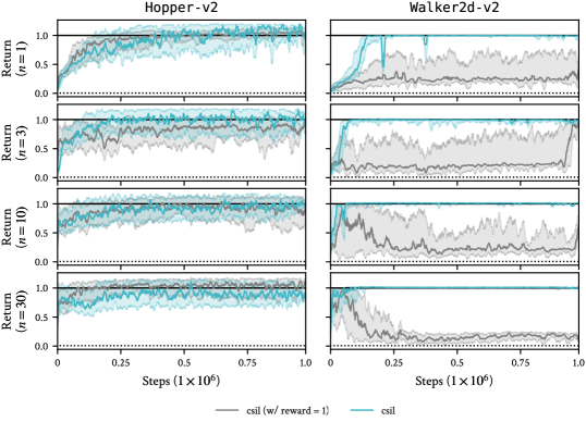
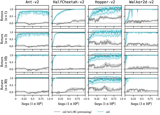
In this setting, we used dac (actor-critic gail), iqlearn, ppil, sqil, and pwil as entropy-regularized imitation learning baselines. We evaluate on the standard benchmark of locomotion-based Gym tasks, using the sac expert data generated by Orsini et al. [2021]. In this setting, Figures 4 and 28 show csil closely matches the best baseline performance across environments and dataset sizes. We also evaluate on the Adroit environments, which involve manipulation tasks with a complex 27-dimensional robot hand [Rajeswaran et al., 2018]. In this setting, Figures 5 and 29 show that saddle-point methods struggle due to the instability of the optimization in high dimensions without careful regularization and hyperparameter selection [Orsini et al., 2021]. In contrast, csil is very effective, matching or surpassing bc, highlighting the benefit of coherency for both policy initialization and improvement. In the Appendix, Figure 29 includes sac from demonstrations (sacfd) [Vecerik et al., 2017, Rajeswaran et al., 2018] as an oracle baseline with access to the true reward. csil exhibits greater sample efficiency than sacfd, presumably due to the bc initialization and the shaped reward, and often matches final performance. Figures 38, 39 and 40 in the Appendix show an ablation of iqlearn and ppil with bc pre-training. We observe a fast unlearning of the bc policy due to the randomly initialized rewards, which was also observed by Orsini et al. [2021], so any initial performance improvement is negligible or temporary.

Figure 5: Normalized performance of csil against baselines for online imitation learning for Adroit tasks. Uncertainty intervals depict quartiles over ten seeds. To assess convergence across seeds, performance is chosen using the highest filtered 25th percentile of the return during learning.

Offline imitation learning.

Another challenging setting for deep rl is offline learning, where the online interactions are replaced with a static ‘supplementary’ dataset. Note that prior works have used ‘offline’ learning to describe the setting where only the demonstrations are used for learning [Kostrikov et al., 2020, Arenz and Neumann, 2020, Garg et al., 2021, Viano et al., 2022], like in bc, such that the il method becomes a form of regularized bc [Ziniu et al., 2022]. Standard offline learning is challenging primarily because the critic approximation can favor unseen actions, motivating appropriate regularization (e.g., [Kumar et al., 2020]). We use the full-replay datasets from the d4rl benchmark [Fu et al., 2020] of the Gym locomotion tasks for the offline dataset, so the offline and demonstration data is not the same. We also evaluate smodice [Ma et al., 2022] and demodice [Kim et al., 2022], two offline imitation learning methods which use state-based value functions, weighted bc policy updates, and a discriminator-based reward. We opt not to reproduce them in acme and use the original implementations. As a consequence, the demonstrations are from a different dataset, but are normalized appropriately. For further details on smodice and demodice, see Appendix A and L.

Figures 6 and 30 demonstrate that offline learning is significantly harder than online learning, with no method solving the tasks with few demonstrations. This can be attributed to the lack of overlap between the offline and demonstration data manifesting as a sparse reward signal. However, with more demonstrations, csil can achieve reasonable performance. This performance is partly due to the strength of the initial bc policy, but csil can still demonstrate policy improvement in some cases (Figure 40). Figure 30 includes cql [Kumar et al., 2020] as an oracle baseline, which has access to the true reward function. For some environments, csil outperforms cql with enough demonstrations. The demodice and smodice baselines are both strong, especially for few demonstrations. However, performance does not increase so much with more demonstrations. Since csil could also be implemented with a state-based value function and a weighed bc policy update (e.g., [Abdolmaleki et al., 2018]), further work is needed to determine which components matter most for effective offline imitation learning.

Figure 6: Normalized performance of csil against baselines for offline imitation learning for Gym tasks. Uncertainty intervals depict quartiles over ten seeds. To assess convergence across seeds, performance is chosen using the highest filtered 25th percentile of the episode return during learning.

5.3 Continuous control from human demonstrations from states and images

Figure 7: Average success rate over 50 evaluations for online imitation learning for robomimic tasks. Uncertainty intervals depict quartiles over ten seeds. To assess convergence across seeds, performance is chosen using the highest 25th percentile of the averaged success during learning.

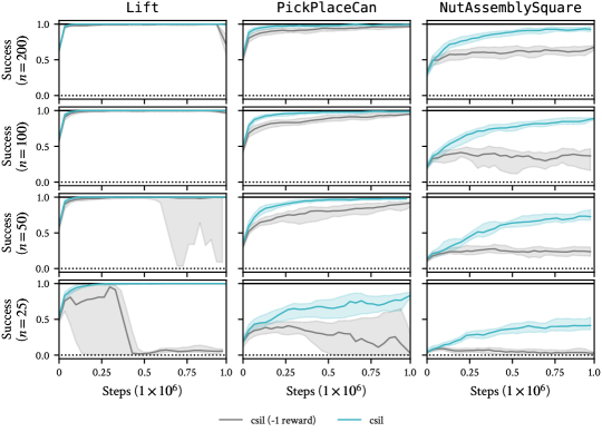
As a more realistic evaluation, we consider learning robot manipulation tasks such as picking (Lift), pick-and-place (PickPlaceCan), and insertion (NutAssemblySquare) from random initializations and mixed-quality human demonstrations using the robomimic datasets [Mandlekar et al., 2021], which also include image observations. The investigation of Mandlekar et al. [2021] considered offline rl and various forms of bc with extensive model selection. Instead, we investigate the applicability of imitation learning, using online learning with csil as an alternative to bc model selection. One aspect of these tasks is that they have a sparse reward based on success, which can be used to define an absorbing state. As observed in prior work [Kostrikov et al., 2019], in practice there is a synergy between absorbing states and the sign of the reward, where positive rewards encourage survival and negative rewards encourage minimum-time strategies. We found that csil was initially ill-suited to these goal-oriented tasks as the rewards are typically positive. In the same way that the airl reward can be designed for a given sign [Orsini et al., 2021], we can design negative csil rewards by deriving an upper-bound of the log policy ratio and subtracting it in the reward. For further details, see Appendix F. An ablation study in Appendix N.9 shows that the negative csil reward matches or outperforms a constant negative reward, especially when given fewer demonstrations. These tasks are also more difficult due to the variance in the initial state, requiring much larger function approximators than in Section 5.2.

Figures 7 and 36 show the performance of csil and baselines, where up to 200 demonstrations are required to sufficiently solve the tasks. csil achieves effective performance and reasonable demonstration sample efficiency across all environments, while baselines such as dac struggle to solve the harder tasks. Moreover, Figure 36 shows csil is again more sample efficient than sacfd.

Figure 8 shows the performance on csil when using image-based observations. A shared cnn torso is used between the policy, reward and critic, and the convolutional layers are frozen after the bc stage. csil was able to solve the simpler tasks in this setting, matching the model selection strategy of Mandlekar et al. [2021], demonstrating its scalability. In the offline setting, Figure 37 shows state-based results with sub-optimal (‘mixed human’) demonstrations as supplementary dataset. While some improvement could be made on simpler tasks, on the whole it appears much harder to learn from suboptimal human demonstrations offline. This supports previous observations that human behaviour can be significantly different to that of rl agents, such that imitation performance is affected [Orsini et al., 2021, Mandlekar et al., 2021].

Figure 8: Average success rate over 50 evaluations for image-based online imitation learning for robomimic tasks. Uncertainty intervals depict quartiles over five seeds. Baseline results obtained from Mandlekar et al. [2021]. bc (csil) denotes the performance of csil’s initial policy for comparison.

6 Discussion

We have shown that ‘coherency’ is an effective approach to il, combining bc with irl-based finetuning by using a shaped learned reward for which the bc policy is optimal. We have demonstrated the effectiveness of csil empirically across a range of settings, particularly for high-dimensional tasks and offline learning, due to csil leveraging bc for initializing the policy and reward.

In Figure 35 of the Appendix, we investigate why baselines iqlearn and ppil, both similar to csil, struggle in the high-dimensional and offline settings. Firstly, the sensitivity of the saddle-point optimization can be observed in the stability of the expert reward and critic values during learning. Secondly, we observe that the policy optimization does not effectively minimize the bc objective by fitting the expert actions. This suggests that these methods do not necessarily converge to a bc solution and lack the ‘coherence’ quality that csil has that allows it to refine bc policies.

A current practical limitation of csil is understanding when the initial bc policy is viable as a coherent reward. Our empirical results show that csil can solve complex control tasks using only one demonstration, where its bc policy is ineffective. However, if a demonstration-rich bc policy cannot solve the task (e.g., image-based NutAssemblySquare), csil also appears to be unable to solve the task. This suggests there is scope to improve the bc models and learning to make performance more consistent across more complex environments. An avenue for future work is to investigate the performance of csil with richer policy classes beyond mlps, such as recurrent architectures and multi-modal action distributions, to assess the implications of the richer coherent reward and better model sub-optimal human demonstrations.

Appendix A Extended related work

This section discusses the relevant prior literature in more breadth and depth.

Generative adversarial imitation learning (gail) [Ho and Ermon, 2016] combines the game-theoretic irl objective with causal entropy regularization and convex regularization of the reward. This primal optimization problem can be transformed into a dual objective, which has the interpretation of minimizing a divergence between the expert and imitator’s stationary distributions, where the divergence corresponds to the choice of convex reward regularization. Choosing regularization that reduced the reward to a classification problem corresponds to the Jensen-Shannon (JS) divergence. While gail used on-policy rl, dac [Kostrikov et al., 2019] used off-policy actor-critic methods (e.g., sac) in an ad hoc fashion for greater sample efficiency. oril [Zołna et al., 2020] adopts a classification-based reward in the offline setting. Kostrikov et al. [2019] also note that the gail classifier can be used in different forms to produce rewards with different forms. airl [Fu et al., 2018b] highlight that the gail reward is shaped by the dynamics if the mdp following the shaping theory of Ng and Russell [2000], and use additional approximators that disentangle the shaping terms. nail [Arenz and Neumann, 2020] replaces the minimax nature of adversarial learning with a more stable max-max approach using expectation maximization-like optimization on a lower-bound of the kl divergence between policies. Its reward function is defined, as with airl, as the log density ratio of the stationary distributions of the expert and policy, regularized by the causal entropy. Therefore, nail and csil have similar reward structures; however, while csil’s reward can be obtained from bc and prior design, nail requires iterative density ratio estimation during learning. Ghasemipour et al. [2019] investigate the performance of airl with different $f$-divergences and corresponding reward regularization beyond JS such as the forward and reverse kl divergence. Ghasemipour et al. [2019] discuss the connection between the log density ratio, airl, gail and their proposed methods. Ghasemipour et al. [2019] also connect bc to irl, but from the divergence perspective rather than the likelihood perspective, as bc can be cast as the conditional kl divergence between the expert and agent policies.

A separate line of study uses the convex duality in a slightly different fashion for ‘discounted distribution correction estimation’ (dice) methods. valuedice uses the Donsker-Varadhan representation to transform the kl minimization problem into an alternative form and a change of variables to represent the log ratio of the stationary distributions as with an implicit representation using the Bellman operator. However, this alternative form is still a saddle-point problem like gail, but the final objective is more amenable to off-policy optimization. Demodice [Kim et al., 2022] considers the offline setting and incorporates kl-regularization into the dice framework, simplififying optimization. Due to the offline setting, the reward is obtained using a pre-trained classifier. Policy improvement reduces to weighted bc, like in many kl-regularized rl methods [Deisenroth et al., 2013, Abdolmaleki et al., 2018]. Smodice [Ma et al., 2022] is closely related to Demodice, but focuses on matching the state distribution and, therefore, does not rely on expert actions, so the discriminator-based reward depends only on the state.

Inverse soft $Q$-learning (iqlearn) [Garg et al., 2021] combines the game-theoretic irl objective, entropy-regularized actor-critic (sac), convex reward regularization and implicit rewards to perform irl using only the critic by maximizing the expert’s implicit reward. While Garg et al. [2021] claim their method is non-adversarial because it does not use a classifier, it is still derived from the game-theoretic objective. For continuous control, the iqlearn implementation requires shaping the implicit reward using online samples, making learning not so different to gail-based algorithms. Moreover, the implementation replaces the minimization of the initial value with the value evaluated for the expert samples. For sac, in which the value function is computed by evaluating the critic with the current policy, this shapes the critic to have a local maximimum around the expert samples. We found this implementation detail crucial to reproduce the results for a few demonstrations and discuss further in Appendix H.

Proximal point imitation learning (ppil) [Viano et al., 2022] combines the game-theoretic and linear programming forms of irl and entropy-regularized actor-critic rl to derive an effective method with convergence guarantees. Its construction yields a single objective (the dual) for optimizing the reward and critic jointly in a more stable fashion, rather than alternating updates like in dac, and unlike iqlearn, it has an explicit reward model. For continuous control, its implementation builds on sac and iqlearn, including the aforementioned tricks, but with two key differences: an explicit reward function and minimization of the ‘logistic’, rather than squared, Bellman error [Bas-Serrano et al., 2021].

Compared to the works discussed above, csil has two main distinctions. One is the reward hypothesis space in the form of the log policy ratio, derived from kl-regularized rl, as opposed to a classifier-based reward or critic-as-classifier implicit reward. Secondly, the consequence of this coherent reward is that it can be pre-trained using bc, and the bc policy can be used as a reference policy. While bc pre-training could be incorporated into prior methods in an ad-hoc fashion, their optimization objectives do not guarantee that coherency is maintained. This is demonstrated in Figure 35, where iqlearn and ppil combined with bc pre-training and kl regularization do not converge like csil.

Concurrent work, least-squares inverse $Q$-learning (ls-iq) [Al-Hafez et al., 2023], addresses the undocumented regularization of iqlearn by minimizing a mixture divergence, which yields the desired regularization terms and better treatment of absorbing states. The treatment moves away from the entropy-regularized rl view and instead opts for explicit regularization critics.

Szot et al. [2023], in concurrent work, use the bi-level optimization view of irl to optimize the maximum entropy reward through an upper-level behavioral cloning loss using ‘meta’ gradients. This approach achieves coherency through the top-level loss while regularizing the learned reward. However, this approach is restricted to on-policy rl algorithms that directly use the reward rather than actor-critics methods that use a $Q$ function, making it less sample efficient.

Brantley et al. [2020] propose disagreement-regularized imitation learning, which trains an ensemble of policies via bc and uses their predictive variance to define a proxy reward. This work shares the same motivation as csil in achieving coherency and tackling the covariate shift problem. Moreover, using ensembles is similar to csil’s stationary policies, as both models are inspired by Bayesian modeling and provide uncertainty quantification. Unlike csil, the method is not motivated by reward shaping, and the reward is obtained by thresholding the predictive variance to $\pm 1$ rather than assume that the likelihood values are meaningful.

Taranovic et al. [2022] derive an airl formalation from the kl divergence between expert and policy that results in a reward consisting of log policy ratios. However, they use a classifier to estimate these quantities and ignore some policy terms in the implementation.

Swamy et al. [2022] use the bc policy for replay estimation [Rajaraman et al., 2020] and a membership classifier to augment the expert dataset used during irl.

‘Noisy’ bc [Sasaki and Yamashina, 2021] is tangentially related to csil, as it uses the bc log-likelihood as a proxy reward to finetune the bc policy using policy gradient updates when learning from demonstrations that are sub-optimal due to additive noise.

Soft $Q$-imitation learning (sqil) [Reddy et al., 2019] uses binary rewards for the demonstration and interaction transitions, bypassing the complexity of standard irl. The benefit of this approach comes from the critic learning to overcome the covariate shift problem through the credit assignment. This approach has no theoretical guarantees, and the simplistic nature of the reward does not encourage stable convergence in practice.

Barde et al. [2020] proposed adversarial soft advantage fitting (asaf), an adversarial approach that constructs the classifier using two policies over trajectories or transitions. This approach is attractive as the classification step performs the policy update, so no policy evaluation step is required. While this approach has clear connections to regularized behavioral cloning, it’s uncertain how the policy learns to overcome covariate shift without any credit assignment. Moreover, this method has no convergence guarantees.

csil adopts a Bayesian-style approach to its initial bc policy by specifying a prior policy but uses the predictive distribution rather than a likelihood to fit the demonstration data. This is in contrast to Bayesian irl [Ramachandran and Amir, 2007], where the prior is placed over the reward function as a means of reasoning about its ambiguity. As the reward is an unobserved abstract quantity, the exponentiated critic is adopted as a pseudo-likelihood, and approximate inference is required to estimate the posterior reward. Using a pseudo-likelihood means that Bayesian irl and me-irl are not so different in practice, especially when using point estimates of the posterior [Choi and Kim, 2011].

Appendix B Likelihoods and priors in imitation learning

The pseudo-posterior perspective in this work was inspired by van Campenhout and Cover [1981], who identify that effective likelihoods arise from relevant functions that describe a distribution. With this in mind, we believe it is useful to see irl as extending bc from a myopic, state-independent likelihood to one that encodes the causal, state-dependent nature of the problem as done me-irl, essentially incorporating the structure of the mdp into the regression problem [Neu and Szepesvári, 2007]. This perspective has two key consequences. One is the importance of the prior, which provides important regularization. For example, Ziniu et al. [2022] have previously shown that the valuedice does not necessarily outperform bc as previously reported but matches bc with appropriate regularization. Moreover, the mimic-exp formulation of bc of Rajaraman et al. [2020] proposes a bc policy with a stationary prior,

$$\pi({\bm{a}}\mid{\bm{s}})=\begin{cases}p_{\mathcal{D}}({\bm{a}}\mid{\bm{s}})\text{ if }{\bm{s}}\in{\mathcal{D}},\text{ where $p_{\mathcal{D}}$ denotes conditional density estimation of ${\mathcal{D}}$,}\\ {\mathcal{U}}_{\mathcal{A}}({\bm{a}})\text{ otherwise.}\end{cases}$$

This work shows how policies like these can be implemented for continuous control using stationary architectures.

The second consequence is the open question of how to define effective likelihoods for imitation learning. me-irl and other prior works use feature matching, which, while an appropriate constraint, raises the additional question of which features are needed. Using a classifier in airl has proved highly effective, but it is not always straightforward to implement in practice without regularization and hyperparameter tuning. Much of iqlearn’s empirical success for continuous tasks arises from shaping the likelihood via the critic through the expert and on-policy regularization terms.

This work addresses the likelihood design problem through coherence and the inversion analysis in Theorem 1, which informs the function-approximated critic regularization described in Section 4. An open question is how these design choices could be further improved, as the ablation study in Figure 46 shows that the benefit of the critic regularization is not evident for all tasks.

Appendix C Parametric stationary processes

The effectiveness of csil is down to its stationary policy design. This section briefly summarizes the definition of stationary processes and how they can be approximated with mlps following the work of Meronen et al. [2021].

While typically discussed for temporal stochastic processes whose input is time, stationary processes (Definition 3) are those whose statistics do not vary with their input. In machine learning, these processes are useful as they allow us to design priors that are consistent per input but capture correlations (e.g., smoothness) across inputs, which can be used for regularization in regression and classification [Rasmussen and Williams, 2006]. In the continuous setting, stationarity can be defined for linear models, i.e., ${y={\bm{w}}^{\top}{\bm{\phi}}({\bm{x}})}$, ${{\bm{w}}\sim{\mathcal{N}}({\bm{\mu}},{\bm{\Sigma}})}$, through their kernel function ${\mathcal{K}}({\bm{x}},{\bm{x}}^{\prime})={\bm{\phi}}({\bm{x}})^{\top}{\bm{\phi}}({\bm{x}}^{\prime})$, the feature inner product. For stationary kernels, the kernel depends only on a relative shift ${\bm{r}}\in{\mathbb{R}}^{d}$ between inputs, i.e. ${\mathcal{K}}({\bm{r}})={\bm{\phi}}({\bm{x}})^{\top}{\bm{\phi}}({\bm{x}}+{\bm{r}})$. By combining the kernel with the weight prior of the linear model, we can define the covariance function, e.g. ${\mathcal{C}}({\bm{r}})={\bm{\phi}}({\bm{x}})^{\top}\,{\bm{\Sigma}}\,{\bm{\phi}}({\bm{x}}+{\bm{r}})$. Boschner’s theorem [Da Prato and Zabczyk, 2014] states that the covariance function of a stationary process can be represented as the Fourier transform of a positive finite measure. If the measure has a density, it is known as the spectral density $S(\bm{\omega})$, and it is a Fourier dual of the covariance function if the necessary conditions apply, known as the Wiener-Khinchin theorem [Chatfield, 1989],

$${\mathcal{C}}({\bm{r}})=\frac{1}{(2\pi)^{d}}\int_{{\mathbb{R}}^{d}}S(\bm{\omega})\exp(i\bm{\omega}^{\top}{\bm{r}})\,{\textnormal{d}}{\bm{r}},\quad S(\bm{\omega})=\int_{{\mathbb{R}}^{d}}{\mathcal{C}}({\bm{r}})\exp(-i\bm{\omega}^{\top}{\bm{r}})\,{\textnormal{d}}\bm{\omega}.$$ (9)

To use this theory to design stationary function approximators, we can use the Wiener-Khintchin theorem to design function approximators that produce a Monte Carlo approximation of stationary kernels. Firstly, we consider only the last layer of the mlp, such that it can be viewed as a linear model. Secondly, Meronen et al. [2021] describe several periodic activation functions that produce products of the form $\exp(i\omega^{\top}{\bm{r}})$, such that the inner product of the whole feature space performs a Monte Carlo approximation of the integral. We implemented sinusoidal, triangular, and periodic ReLU activations (see Figure 3 of Meronen et al. [2021]) as a policy architecture hyperparameter. Thirdly, the input into the stationary kernel approximation should be small (e.g., $<20$), as the stationary behavior is dictated by ${\bm{r}}$, and this distance becomes less meaningful in higher dimensions. This means the mlp feature space that feeds into the last layer should be small or have a ‘bottleneck’ architecture to compress the internal representation. Finally, we require a density to represent the spectral density, which also defines the nature of the stationary process. We use a Gaussian, but other distributions such as a Student-$t$ or Cauchy could be used if ‘rougher’ processes are desired. In summary, the last layer activations take the form $f_{p}({\bm{W}}{\bm{\phi}}({\bm{x}})),$ where $f_{p}$ is the periodic activation function of choice, ${\bm{W}}$ are weights sampled from the distribution of choice and ${\bm{\phi}}({\bm{x}})$ is an arbitrary (but bottlenecked) mlp feature space of choice.

Related work combining stationary kernel approximations with mlps have constrained the feature space with a residual architecture and spectral normalization to bound the upper and lower Lipschitz constant [Liu et al., 2020], to prevent these features overfitting. We found we did not need this to achieve approximate stationarity (e.g., Figure 3), which avoided the need for input-dependent policy architectures which may lead to a risk of underfitting.

A crucial practical detail is that the sampled weights ${\bm{W}}$ should be trained and not kept constant, as the theory suggests. In practice, we did not observe the statistics of these weights changing significantly during training, while training this weight layer reduced underfitting enough for substantially more effective bc performance.

Appendix D Faithful heteroscedastic regression

Figure 9: We repeat the regression problem from Figure 3 to highlight the effect of ‘faithful’ heteroscedastic regression. The nllh objective has a tendency to model ‘signal’ as noise, which is most clearly seen in the heteroscedastic mlp. The faithful heteroscedastic loss reduces the mean prediction error significantly without affecting uncertainty quantification for both models.

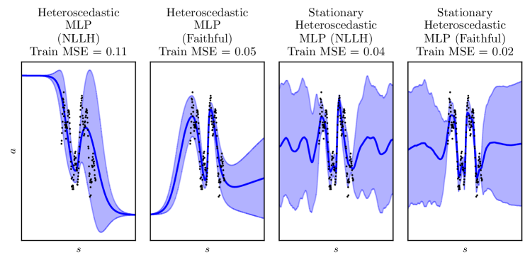
This section summarizes the approach of Stirn et al. [2023]. The faithful objective combines the mean squared error (mse) and negative log-likelihood nllh loss with a careful construction of the heteroscedastic model. The loss is

$${\mathcal{L}}({\mathcal{D}},{\bm{\theta}}) =\mathbb{E}_{{\bm{s}},{\bm{a}}\sim{\mathcal{D}}}\left[({\bm{a}}-{\bm{\mu}}_{\bm{\theta}}({\bm{s}}))^{2}-\log\tilde{q}({\bm{a}}\mid{\bm{s}})\right],\quad\tilde{q}({\bm{a}}\mid{\bm{s}})={\mathcal{N}}(\text{{sg}}({\bm{\mu}}_{\bm{\theta}}({\bm{s}})),{\bm{\Sigma}}_{\bm{\theta}}({\bm{s}})),$$ (10)

where $\text{{sg}}(\cdot)$ denotes the stop gradient operator. Moreover, for the models ‘shared torso’ (e.g., features), the gradient is stopped between the torso and the predictive variance so that the features are only trained to satisfy the MSE objective. Figure 9 illustrates the impact of the alternative loss function and model adjustments. Note that the faithful objective is not strictly necessary for bc or csil and is mitigating potential under-fitting previously observed empirically. The issue of modeling ‘signal’ as noise when using heteroscedastic function approximators is poorly understood and depends on the model architecture, initialization, and the dataset considered. While motivated by 1D toy examples, it was observed during development that the faithful objective is beneficial for csil’s downstream performance.

Appendix E Reward refinement and function-space relative entropy estimation

In the function approximation setting, we refine the reward model with additional non-expert samples. Motivated by Theorem 2, we maximize the objective using samples from the replay buffers

$${\mathcal{J}}_{r}({\bm{\theta}})=\mathbb{E}_{{\bm{s}},{\bm{a}}\sim{\mathcal{D}}}\left[\alpha\log\frac{q_{\bm{\theta}}({\bm{a}}\mid{\bm{s}})}{p({\bm{a}}\mid{\bm{s}})}\right]-\mathbb{E}_{{\bm{s}},{\bm{a}}\sim\rho_{\pi}}\left[\alpha\log\frac{q_{\bm{\theta}}({\bm{a}}\mid{\bm{s}})}{p({\bm{a}}\mid{\bm{s}})}\right].$$ (11)

If the behavior policy $\pi$ is $q_{\bm{\theta}}({\bm{a}}\mid{\bm{s}})$, we can view the second term as a Monte Carlo estimation of the relative KL divergence between $q$ and $p$. This estimator can suffer greatly from bias, as the KL should always be non-negative. To counteract this, we construct an unbiased, positively-constrained estimator following Schulman [2020], using $\mathbb{E}_{{\bm{x}}\sim q(\cdot)}[R({\bm{x}})^{-1}]=\int p({\bm{x}})\,{\textnormal{d}}{\bm{x}}=1$ and $\log(x)\leq x-1$,

$$\mathbb{D}_{\textsc{kl}}[q({\bm{x}})\mid\mid p({\bm{x}})]=\mathbb{E}_{{\bm{x}}\sim q(\cdot)}[\log R({\bm{x}})]=\mathbb{E}_{{\bm{x}}\sim q(\cdot)}[R({\bm{x}})^{-1}-1+\log R({\bm{x}})],$$

This estimator results in replacing the second term of Equation 11 with

$$\mathbb{E}_{{\bm{s}},{\bm{a}}\sim\rho_{\pi}}\left[r_{\bm{\theta}}({\bm{s}},{\bm{a}})\right]\rightarrow\mathbb{E}_{{\bm{s}},{\bm{a}}\sim\rho_{\pi}}\left[r_{\bm{\theta}}({\bm{s}},{\bm{a}})-1+\exp(-r_{\bm{\theta}}({\bm{s}},{\bm{a}}))\right].$$ (12)

This objective is maximized concurrently with policy evaluation, using samples from the replay buffer. This reward refinement is similar to behavioral cloning via function-space variational inference (e.g., [Sun et al., 2019, Watson et al., 2021]), enforcing the prior using the prior predictive distribution rather than the prior weight distribution. We found that applying the estimator to the scaled log ratio (Equation 12) lead to better downstream performance empirically than scaling the estimator applied to the log ratio.

In practice, the samples are taken from a replay buffer of online and offline data, so the action samples are taken from a different distribution to $q_{\bm{\theta}}$. However, we still found the adjusted objective effective for reward regularization. Without it, the saddle-point refinement was less stable. Appendix G illustrates this refinement in a simple setting. Figure 45 ablates this component, where its effect is most beneficial when there are fewer demonstrations.

Appendix F Bounding the coherent reward

The coherent reward $\alpha(\log q({\bm{a}}\mid{\bm{s}})-\log p({\bm{a}}\mid{\bm{s}}))$ can be upper bounded if $p({\bm{a}}\mid{\bm{s}})>0$ whenever $q({\bm{a}}\mid{\bm{s}})>0$. The bound is policy dependent. We use the bound in the continuous setting, where we use a tanh-transformed Gaussian policy. We add a small bias term $\sigma^{2}_{\text{min}}$ to the predictive variance in order to define the Gaussian likelihood upper bound. Inconveniently, the tanh change of variables term in the log-likelihood $-\sum_{i=1}^{d_{a}}\log(1-\text{tanh}^{2}(u))$ [Haarnoja et al., 2018] has no upper bound in theory, as the ‘latent’ action $u\in[-\infty,\infty]$, but in the Acme implementation this log-likelihood is bounded for numerical stability due to the inverse tanh operation. For action dimension $d_{a}$ and uniform prior across action range $[-1,1]^{d_{a}}$ and $\alpha=d_{a}^{-1}$, the upper bound is $r({\bm{s}},{\bm{a}})\leq\frac{1}{d_{a}}(-0.5d_{a}\log 2\pi\sigma^{2}_{\text{min}}+c+d_{a}\log 2)=-0.5\log\pi\sigma^{2}_{\text{min}}/2+\tilde{c}$, where $c,\tilde{c}$ depends on the tanh clipping term.

Figure 10: We extend the regression problem from Figure 3 to highlight the effect of reward refinement detailed in Section E from the bc and irl perspective. Refining the coherent reward with a minimax objective results in a bc policy that appears more stationary, as seen in the heteroscedatic mlp. The stationary heteroscedastic policy is also refined, but to a lesser degree, as it’s approximately stationary by construction. The colourmap is shared between contour plots, and rewards are clipped at -10 to improve the visual colour range. Regression uncertainty is one standard deviation.

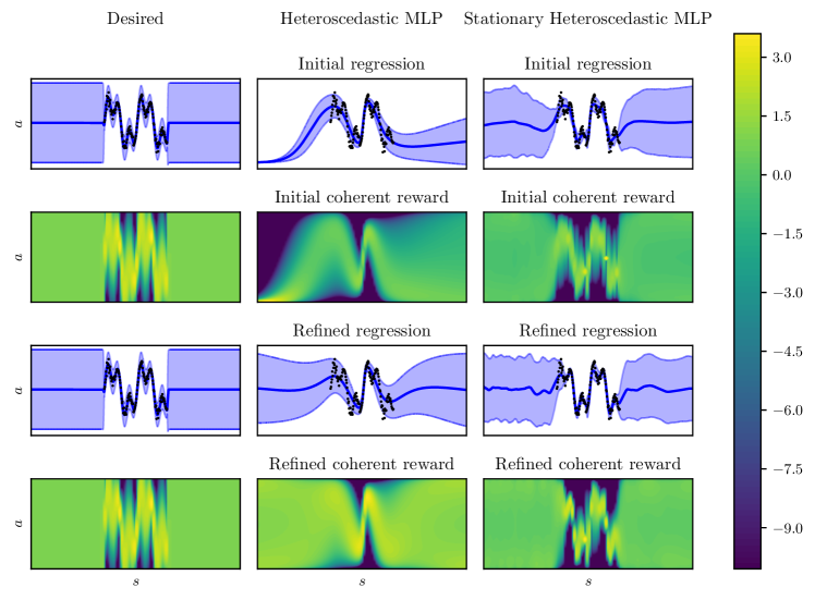
Appendix G Visualizing reward refinement

To provide intuition on Theorem 2 and connect it to reward refinement (Appendix E), we build on the regression example from Figure 3 by viewing it as a continuous contextual bandit problem, i.e., a single-state mdp with no dynamics. Outside of the demonstration state distribution, we desire that the reward is uniformly zero, as we have no data to inform action preference. Figure 10 shows the result of applying csil and reward refinement to this mdp, where the state distribution is uniform. The ‘desired’ bc fit exhibits a coherent reward with the desired qualities, and the hetstat policy approximates this desired policy. The heteroscedastic mlp exhibits undesirable out-of-distribution (OOD) behavior, where arbitrary regions have strongly positive or negative rewards. Reward refinement improves the coherent reward of the heteroscedastic mlp to be more uniform OOD, which in turn makes the regression fit look more like a stationary policy. This result reinforces Theorem 2, which shows that kl-regularized bc is connected to a lower bound on an entropy-regularized game-theoretic irl objective that uses the coherent reward.

Appendix H Critic regularization

Figure 11: Illustrating the two forms of critic regularization on a toy 1D problem for critic ${\mathcal{Q}}(a)$ with regression target . Jacobian regularization minimizes the squared gradient and corresponds to csil. Sample regularization minimizes sampled nearby actions and corresponds to iqlearn and ppil. Both approaches shape the critic to have zero gradient around the target action, denoted by the dotted lines. A standard two-layer mlp with 256 units and elu actions is used for approximation.

For the function approximation setting, csil requires an auxiliary loss term during learning to incorporate coherency. The full critic optimization problem is $\textstyle\min_{\bm{\phi}}{\mathcal{J}}_{\mathcal{Q}}({\bm{\phi}})$ for objective

$${\mathcal{J}}_{\mathcal{Q}}({\bm{\phi}})=\mathbb{E}_{{\bm{s}},{\bm{a}}\sim{\mathcal{B}}}[({\mathcal{Q}}_{\bm{\phi}}({\bm{s}},{\bm{a}})-{\mathcal{Q}}^{*}({\bm{s}},{\bm{a}}))^{2}]+\mathbb{E}_{{\bm{s}},{\bm{a}}\sim{\mathcal{D}}}[|\nabla_{\bm{a}}{\mathcal{Q}}_{\bm{\phi}}({\bm{s}},{\bm{a}})|^{2}],$$ (13)

where ${\mathcal{Q}}^{*}$ denotes the target $Q$ values and ${\mathcal{B}}$ denotes the replay buffer, that combines demonstrations ${\mathcal{D}}$ and additional samples. The motivation is to shape the critic such that the demonstration actions are first-order optimal by minimizing the squared Frobenius norm of the action Jacobian.

iqlearn and ppil adopt similar, but less explicit, regularization. Equation 10 of Garg et al. [2021] is

$$\textstyle\max_{\bm{\phi}}\mathbb{E}_{{\bm{s}},{\bm{a}}\sim{\mathcal{B}}}\left[f\left({\mathcal{Q}}_{\bm{\phi}}({\bm{s}},{\bm{a}})-\gamma\,\mathbb{E}_{{\bm{s}}^{\prime}\sim{\mathcal{P}}(\cdot\mid{\bm{s}},{\bm{a}})}[{\mathcal{V}}_{\bm{\phi}}^{\pi}({\bm{s}}^{\prime})]\right)\right]-(1-\gamma)\mathbb{E}_{{\bm{s}}\sim\mu_{0}}[{\mathcal{V}}_{\bm{\phi}}^{\pi}({\bm{s}})],$$

where ${\mathcal{V}}_{\bm{\phi}}^{\pi}({\bm{s}})={\mathcal{Q}}({\bm{s}},{\bm{a}}^{\prime})$, ${\bm{a}}^{\prime}\sim\pi(\cdot\mid{\bm{s}})$ and $f$ is the concave function defining the implicit reward regularization. In the implementation [Div99, 2021], the ‘v0’ objective variant replaces the initial distribution $\mu_{0}$ with the demonstration state distribution. This trick is deployed to improve regularization without affecting optimality (Section 5.3, Kostrikov et al. [2020]). If the policy matches the expert actions with its mode, this term shapes a local maximum by minimizing the critic at action samples around the expert. However, if the policy does not accurately match the expert actions, the effect of this term is harder to reason about. In Figure 11, we illustrate these two forms from critic regularization on a toy example, demonstrating that both can produce local maximums in the critic.

Appendix I Practical algorithm with function approximation

For deep imitation learning, csil adopts sac for the spi step in Algorithm 1, summarized in Algorithm 2. The critic objective for both pre-training and policy evaluation is the squared Bellman error. The policy objective $\max_{\bm{\theta}}{\mathcal{J}}_{\pi}({\bm{\theta}})$ samples both the demonstrations and replay buffer,

$${\mathcal{J}}_{\pi}({\bm{\theta}})=E_{{\bm{a}}\sim q_{\bm{\theta}}(\cdot\mid{\bm{s}}),\,{\bm{s}}\sim{\mathcal{B}}\,\cup\,{\mathcal{D}}}\left[{\mathcal{Q}}({\bm{s}},{\bm{a}})-\beta(\log q_{\bm{\theta}}(\cdot\mid{\bm{s}})-\log q_{{\bm{\theta}}_{1}}(\cdot\mid{\bm{s}}))\right].$$ (14)

The policy and demonstration data are combined equally. We did not experiment with tuning this ratio. Compared to sac, we found we did not have to train multiple critics, but we did need target networks for the critics to stabilize learning. The critic and reward objectives were also evaluated on the policy and expert data each update. Moreover, like iqlearn and ppil, we kept $\beta$ constant and did not use an adaptive strategy.

Data: Expert demonstrations ${\mathcal{D}}$, initial temperature $\alpha$, refinement temperature, $\beta$,

parametric policy class $q_{\bm{\theta}}({\bm{a}}\mid{\bm{s}})$, prior policy $p({\bm{a}}\mid{\bm{s}})$, regression regularizer $\Psi$, total steps $T$

Result: $q_{{\bm{\theta}}_{N}}({\bm{a}}\mid{\bm{s}})$, matching or improving the initial policy $q_{{\bm{\theta}}_{1}}({\bm{a}}\mid{\bm{s}})$

// Pretrain coherent reward and critic

Train initial policy from demonstrations, ${\bm{\theta}}_{1}=\operatorname*{arg\,max}_{{\bm{\theta}}}\mathbb{E}_{{\bm{s}},{\bm{a}}\sim{\mathcal{D}}}[\log q_{\bm{\theta}}({\bm{a}}\mid{\bm{s}})-\Psi({\bm{\theta}})]$;

Define fixed shaped coherent reward, $\tilde{r}_{{\bm{\theta}}_{1}}({\bm{s}},{\bm{a}})=\alpha(\log q_{{\bm{\theta}}_{1}}({\bm{a}}\mid{\bm{s}})-\log p({\bm{a}}\mid{\bm{s}}))$;

Pretrain critic with SARSA on ${\mathcal{D}}$ using $\tilde{r}_{{\bm{\theta}}_{1}}$.

for $t=1\rightarrow T$ do // finetune policy with reinforcement learning

       Interact with environment ${\bm{s}}_{t+1}=\text{{Env}}({\bm{s}}_{t},{\bm{a}}_{t})$, ${\bm{a}}_{t}\sim q_{{\bm{\theta}}_{t}}(\cdot\mid{\bm{s}}_{t})$, store in replay buffer ${\mathcal{B}}$;

       Optimize reward and critic using ${\mathcal{J}}_{\mathcal{Q}}({\bm{\phi}})$ and ${\mathcal{J}}_{r}({\bm{\theta}})$ (Equations 13, 11) on minibatch from ${\mathcal{B}}$;

       Update policy optimizing ${\mathcal{J}}_{\pi}({\bm{\theta}})$ (Equation 14) on minibatch from ${\mathcal{B}}$;

      

end for

Algorithm 2 Off-policy coherent soft imitation learning with function approximation

Appendix J A divergence minimization perspective

Many imitation learning algorithms, such as gail and iqlearn, are derived from minimizing a divergence between the agent’s state-action distribution and the expert’s. While csil is derived through policy inversion, it also has a divergence minimization perspective, albeit with two minimization steps rather than one.

The first step involves recognising that maximum likelihood bc fit minimizes the forward kl divergence between the demonstration distribution $p_{\mathcal{D}}({\bm{s}},{\bm{a}})=p_{\mathcal{D}}({\bm{a}}\mid{\bm{s}})\,p_{\mathcal{D}}({\bm{s}})$ and the policy,

$${\bm{\theta}}_{1}=\textstyle\operatorname*{arg\,min}_{\bm{\theta}}\mathbb{E}_{{\bm{s}}\sim p_{\mathcal{D}}(\cdot)}[\mathbb{D}_{\textsc{kl}}[p_{\mathcal{D}}({\bm{a}}\mid{\bm{s}})\mid\mid q_{\bm{\theta}}({\bm{a}}\mid{\bm{s}})]]=\operatorname*{arg\,max}_{\bm{\theta}}\mathbb{E}_{{\bm{s}},{\bm{a}}\sim{\mathcal{D}}}[\log q_{\bm{\theta}}({\bm{a}}\mid{\bm{s}})].$$

Using the forward kl means that the unknown log-likelihood of the data distribution is not required, and the policy can be trained using supervised learning and without environment interaction.

The second step involves rearranging the kl-regularized rl objective into two kl divergences,

$${\bm{\theta}}_{*} =\textstyle\operatorname*{arg\,max}_{{\bm{\theta}}}\mathbb{E}_{{\bm{a}}\sim q_{\bm{\theta}}(\cdot\mid{\bm{s}}),\,{\bm{s}}\sim\mu_{\pi_{\bm{\theta}}}(\cdot)}\left[\alpha\log\frac{q_{{\bm{\theta}}_{1}}({\bm{a}}\mid{\bm{s}})}{p({\bm{a}}\mid{\bm{s}})}-\beta\log\frac{q_{\bm{\theta}}({\bm{a}}\mid{\bm{s}})}{p({\bm{a}}\mid{\bm{s}})}\right],$$

$$=\textstyle\operatorname*{arg\,min}_{q_{\bm{\theta}}}\mathbb{E}_{{\bm{s}}\sim\mu_{q_{\bm{\theta}}}(\cdot)}[\alpha\,\mathbb{D}_{\textsc{kl}}[q_{\bm{\theta}}({\bm{a}}\mid{\bm{s}})\mid\mid q_{{\bm{\theta}}_{1}}({\bm{a}}\mid{\bm{s}})]-(1-\beta/\alpha)\,\mathbb{D}_{\textsc{kl}}[q_{\bm{\theta}}({\bm{a}}\mid{\bm{s}})\mid\mid p({\bm{a}}\mid{\bm{s}})]].$$

Note that since $\beta\leq\alpha$, then $(1-\beta/\alpha)\geq 0$. The left-hand term minimizes the reverse kl between the agent and the expert, using the bc policy as a proxy. This is beneficial because the reverse conditional kl requires evaluating policy $q_{\bm{\theta}}$ on the environment. Moreover, the reverse kl requires log-likelihoods of the target distribution, which is why the bc policy is used as a proxy of the demonstration distribution. The right-hand term incorporates the coherent reward and encourages the policy to stay in states where the policy differs from the prior. As $q_{\bm{\theta}}$ should be close to the bc policy due to the left-hand term, the coherent reward shaping from Definition 1 should hold.

In this formulation of the objective, it is also clear to see that if $\beta=\alpha$, no rl finetuning will occur, and $q_{\bm{\theta}}$ will simply mimic the bc policy $q_{{\bm{\theta}}_{1}}$ due to the left-hand term.

Appendix K Theoretical results

This section provides derivations and proofs for the theoretical results in the main text.

K.1 Relative entropy regularization for reinforcement learning

This section re-derives kl-regularized rl and me-irl in a shared notation for the reader’s reference.

Reinforcement learning.

We consider the discounted, infinite-horizon setting with a hard kl constraint on the policy update with bound $\epsilon$,

$$\textstyle\max_{q}\mathbb{E}_{{\bm{s}}_{t+1}\sim{\mathcal{P}}(\cdot\mid{\bm{s}}_{t},{\bm{a}}_{t}),\,{\bm{a}}_{t}\sim q(\cdot\mid{\bm{s}}_{t}),\,{\bm{s}}_{0}\sim\mu_{0}(\cdot)}[\sum_{t}\gamma^{t}r({\bm{s}}_{t},{\bm{a}}_{t})]\quad\text{s.t.}\quad\mathbb{E}_{{\bm{s}}\sim\nu_{q}(\cdot)}[\mathbb{D}_{\textsc{kl}}[q({\bm{a}}\mid{\bm{s}})\mid\mid p({\bm{a}}\mid{\bm{s}})]]\leq\epsilon.$$

This constrained objective is transcribed into the following Lagrangian objective following Van Hoof et al. [2017], using the discounted stationary joint distribution $d({\bm{s}},{\bm{a}})=q({\bm{a}}\mid{\bm{s}})\,\nu({\bm{s}})=(1-\gamma)\rho({\bm{s}},{\bm{a}})$,

$${\mathcal{L}}(d,\lambda_{1},\lambda_{2},\lambda_{3}) =(1-\gamma)^{-1}\int_{{\mathcal{S}}\times{\mathcal{A}}}d({\bm{s}},{\bm{a}})\,r({\bm{s}},{\bm{a}})\,{\textnormal{d}}{\bm{s}}\,{\textnormal{d}}{\bm{a}}+\lambda_{1}\left(1-\int_{{\mathcal{S}}\times{\mathcal{A}}}d({\bm{s}},{\bm{a}})\,{\textnormal{d}}{\bm{s}}\,{\textnormal{d}}{\bm{a}}\right)$$

$$+\int_{{\mathcal{S}}}\lambda_{2}({\bm{s}}^{\prime})\left(\int_{{\mathcal{S}}\times{\mathcal{A}}}\gamma\,{\mathcal{P}}({\bm{s}}^{\prime}\mid{\bm{s}},{\bm{a}})\,d({\bm{s}},{\bm{a}})\,{\textnormal{d}}{\bm{s}}\,{\textnormal{d}}{\bm{a}}+(1-\gamma)\mu_{0}({\bm{s}}^{\prime})-\int_{{\mathcal{A}}}d({\bm{s}}^{\prime},{\bm{a}}^{\prime})\,{\textnormal{d}}{\bm{a}}^{\prime}\right)\,{\textnormal{d}}{\bm{s}}^{\prime}$$

$$+\lambda_{3}\left(\epsilon-\int_{\mathcal{S}}\nu({\bm{s}})\int_{\mathcal{A}}q({\bm{a}}\mid{\bm{s}})\log\frac{q({\bm{a}}\mid{\bm{s}})}{p({\bm{a}}\mid{\bm{s}})}\,{\textnormal{d}}{\bm{a}}\,{\textnormal{d}}{\bm{s}}\right),$$

where $$\lambda_{2} \partial{\mathcal{L}}(q,\lambda_{1},\lambda_{2},\lambda_{3})/\partial d=0$$ is a function for an infinite-dimensional constraint. Solving for ,

$$q({\bm{a}}\mid{\bm{s}}) \propto\exp(\alpha^{-1}(\underbrace{r({\bm{s}},{\bm{a}})+\gamma\,\mathbb{E}_{{\bm{s}}^{\prime}\sim{\mathcal{P}}(\cdot\mid{\bm{s}},{\bm{a}})}[{\mathcal{V}}({\bm{s}}^{\prime})]}_{{\mathcal{Q}}({\bm{s}},{\bm{a}})}-{\mathcal{V}}({\bm{s}})))\,p({\bm{a}}\mid{\bm{s}}),$$

with $$\alpha=(1-\gamma)\lambda_{3} \lambda_{2}({\bm{s}})=(1-\gamma){\mathcal{V}}({\bm{s}}) {\mathcal{V}}$$ and , where can be interpreted as the soft value function,

$${\mathcal{V}}({\bm{s}}) =\alpha\log\int_{\mathcal{A}}\exp\left(\frac{1}{\alpha}\,{\mathcal{Q}}({\bm{s}},{\bm{a}})\right)\,p({\bm{a}}\mid{\bm{s}})\,{\textnormal{d}}{\bm{a}}\quad\text{as}\quad\int_{\mathcal{A}}q({\bm{a}}\mid{\bm{s}})\,{\textnormal{d}}{\bm{a}}=1.$$

To obtain the more convenient lower bound of the soft Bellman equation, we combine importance sampling and Jensen’s inequality to the soft Bellman equation

$${\mathcal{V}}({\bm{s}}) =\alpha\log\int_{\mathcal{A}}\exp\left(\frac{1}{\alpha}\,{\mathcal{Q}}({\bm{s}},{\bm{a}})\right)\,\frac{p({\bm{a}}\mid{\bm{s}})}{q({\bm{a}}\mid{\bm{s}})}\,q({\bm{a}}\mid{\bm{s}})\,{\textnormal{d}}{\bm{a}},$$

$$\geq\mathbb{E}_{{\bm{a}}\sim q(\cdot\mid{\bm{s}})}\left[{\mathcal{Q}}({\bm{s}},{\bm{a}})-\alpha\log\frac{q({\bm{a}}\mid{\bm{s}})}{p({\bm{a}}\mid{\bm{s}})}\right].$$

This derivation is for the ‘hard’ kl constraint. In many implementations, including ours, the constraint is ‘softened’ where $\lambda_{3}$ and, therefore, $\alpha$ is a fixed hyperparameter.

Inverse reinforcement learning.

As mentioned in Section 2 and Definition 2, me-irl is closely related to kl-regularize rl, but with the objective and a constraint reversed,

$$\textstyle\min_{q}\mathbb{E}_{{\bm{s}}\sim\nu_{q}(\cdot)}[\mathbb{D}_{\textsc{kl}}[q({\bm{a}}\mid{\bm{s}})\mid\mid p({\bm{a}}\mid{\bm{s}})]]\quad\text{s.t.}\quad\mathbb{E}_{{\bm{s}},{\bm{a}}\sim\rho_{q}}[{\bm{\phi}}({\bm{s}},{\bm{a}})]=\mathbb{E}_{{\bm{s}},{\bm{a}}\sim{\mathcal{D}}}[{\bm{\phi}}({\bm{s}},{\bm{a}})].$$

The constrained optimization is, therefore, transcribed into a similar Lagrangian,

$${\mathcal{L}}(d,\lambda_{1},\lambda_{2},\bm{\lambda_{3}}) =\int_{\mathcal{S}}\nu({\bm{s}})\int q({\bm{a}}\mid{\bm{s}})\log\frac{q({\bm{a}}\mid{\bm{s}})}{p({\bm{a}}\mid{\bm{s}})}\,{\textnormal{d}}{\bm{a}}\,{\textnormal{d}}{\bm{s}}+\lambda_{1}\left(1-\int_{{\mathcal{S}}\times{\mathcal{A}}}d({\bm{s}},{\bm{a}})\,{\textnormal{d}}{\bm{s}}\,{\textnormal{d}}{\bm{a}}\right)$$

$$+\int_{{\mathcal{S}}}\lambda_{2}({\bm{s}}^{\prime})\left(\int_{{\mathcal{S}}\times{\mathcal{A}}}\gamma\,{\mathcal{P}}({\bm{s}}^{\prime}\mid{\bm{s}},{\bm{a}})\,d({\bm{s}},{\bm{a}})\,{\textnormal{d}}{\bm{s}}\,{\textnormal{d}}{\bm{a}}+(1-\gamma)\mu_{0}({\bm{s}}^{\prime})-\int_{{\mathcal{A}}}d({\bm{s}}^{\prime},{\bm{a}}^{\prime})\,{\textnormal{d}}{\bm{a}}^{\prime}\right)\,{\textnormal{d}}{\bm{s}}^{\prime}$$

$$+\bm{\lambda_{3}}^{\top}\left((1-\gamma)^{-1}\int_{{\mathcal{S}}\times{\mathcal{A}}}d({\bm{s}},{\bm{a}})\,{\bm{\phi}}({\bm{s}},{\bm{a}})\,{\textnormal{d}}{\bm{s}}\,{\textnormal{d}}{\bm{a}}-\mathbb{E}_{{\bm{s}},{\bm{a}}\sim{\mathcal{D}}}[{\bm{\phi}}({\bm{s}}_{t},{\bm{a}}_{t})]\right).$$

The consequence of this change is that the likelihood temperature is now implicit in the reward model $r({\bm{s}},{\bm{a}})=(1-\gamma)^{-1}\bm{\lambda_{3}}^{\top}{\bm{\phi}}({\bm{s}},{\bm{a}})$ due to the Lagrange multiplier weights, this reward model is used in the soft Bellman equation instead of the true reward. The reward model is jointly optimized to minimize the apprenticeship error by matching the feature expectation.

K.2 Proof for Theorem 1

See 1

Proof.

Equation 6 is derived by rearranging the posterior policy update in Equation 4. Equation 7 in derived by substituting the critic expression from Equation 6 into the kl-regularized Bellman equation (Equation 3),

$$\underbrace{\alpha\log\frac{q_{\alpha}({\bm{a}}\mid{\bm{s}})}{p({\bm{a}}\mid{\bm{s}})}+{\mathcal{V}}_{\alpha}({\bm{s}})}_{{\mathcal{Q}}({\bm{s}},{\bm{a}})}=\hskip 250.00038pt$$

$$r({\bm{s}},{\bm{a}})+\gamma\,\mathbb{E}_{{\bm{s}}^{\prime}\sim{\mathcal{P}}(\cdot\mid{\bm{s}},{\bm{a}}),\,{\bm{a}}^{\prime}\sim q_{\alpha}(\cdot\mid{\bm{s}}^{\prime})}\left[\underbrace{\cancel{\alpha\log\frac{q_{\alpha}({\bm{a}}^{\prime}\mid{\bm{s}}^{\prime})}{p({\bm{a}}^{\prime}\mid{\bm{s}}^{\prime})}}+{\mathcal{V}}_{\alpha}({\bm{s}}^{\prime})}_{{\mathcal{Q}}({\bm{s}}^{\prime},{\bm{a}}^{\prime})}-\cancel{\alpha\log\frac{q_{\alpha}({\bm{a}}^{\prime}\mid{\bm{s}}^{\prime})}{p({\bm{a}}^{\prime}\mid{\bm{s}}^{\prime})}}\right].$$

∎

K.3 Proof for Theorem 2

Theorem 2 relies on the data processing inequality (Lemma 3) to connect the function-space kl seen in csil with the weight-space kl used in regularized bc.

Assumption 1.

(Realizability) The optimal policy can be expressed by the parametric policy $q_{\bm{\theta}}({\bm{a}}|{\bm{s}})$.

Lemma 2.

(Coherent policy optimality). The optimal policy for a kl-regularized rl problem with coherent reward $\tilde{r}({\bm{s}},{\bm{a}})=\alpha(\log q({\bm{a}}\mid{\bm{s}})-\log p({\bm{a}}\mid{\bm{s}}))$ and temperature $\alpha$ is $q({\bm{a}}\mid{\bm{s}})$.

Proof.

This result arises from the origin of the coherent reward from policy inversion and reward shaping (Theorem 1, Lemma 1). Moreover, considering the entropy-augmented reward ${r_{\alpha,\,\pi}({\bm{s}},{\bm{a}})=r({\bm{s}},{\bm{a}})-\alpha(\log\pi({\bm{a}}\mid{\bm{s}})-\log p({\bm{a}}\mid{\bm{s}})}$, when $r$ is the coherent reward $\tilde{r}$ and $\pi=q$, $\tilde{r}_{\alpha,\,q}({\bm{s}},{\bm{a}})=0\,\forall{\bm{s}}\in{\mathcal{S}},\,{\bm{a}}\in{\mathcal{A}}$ so $q({\bm{a}}\mid{\bm{s}})$ is a solution to a soft policy iteration. ∎

Lemma 3.

(Data processing inequality, Wu [2016], Theorem 4.1). For two stochastic processes parameterized with finite random variables ${\bm{w}}\sim p(\cdot)$, ${\bm{w}}{\,\in\,}{\mathcal{W}}$ and shared hypothesis spaces ${p({\bm{y}}\mid{\bm{x}},{\bm{w}})}$, the conditional $f$-divergence in function space at points ${\bm{X}}\in{\mathcal{X}}^{L},L\in{\mathbb{Z}}_{+}.$ is upper bounded by the $f$-divergence in parameter space,

$${\mathbb{D}}_{f}[q({\bm{w}})\mid\mid p({\bm{w}})]={\mathbb{D}}_{f}[q({\bm{Y}},{\bm{w}}\mid{\bm{X}})\mid\mid p({\bm{Y}},{\bm{w}}\mid{\bm{X}})] \geq{\mathbb{D}}_{f}[q({\bm{Y}}\mid{\bm{X}})\mid\mid p({\bm{Y}}\mid{\bm{X}})].$$

See 2

Proof.

We begin with the kl-regularized game-theoretic irl objective (c.f. Equation 1 [Haarnoja et al., 2018]),

$${\mathcal{J}}(r,\pi,\beta) =\mathbb{E}_{{\bm{s}},{\bm{a}}\sim{\mathcal{D}}}\left[r({\bm{s}},{\bm{a}})\right]-\mathbb{E}_{{\bm{s}},{\bm{a}}\sim\rho_{\pi}}\left[r({\bm{s}},{\bm{a}})-\beta\log\frac{\pi({\bm{a}}\mid{\bm{s}})}{p({\bm{a}}\mid{\bm{s}})}\right].$$

Substituting the coherent reward from Theorem 1, the objective becomes

$${\mathcal{J}}({\bm{\theta}},\pi,\beta) =\mathbb{E}_{{\bm{s}},{\bm{a}}\sim{\mathcal{D}}}\left[\alpha\log\frac{q_{\bm{\theta}}({\bm{a}}\mid{\bm{s}})}{p({\bm{a}}\mid{\bm{s}})}\right]-\mathbb{E}_{{\bm{s}},{\bm{a}}\sim\rho_{\pi}}\left[\alpha\log\frac{q_{\bm{\theta}}({\bm{a}}\mid{\bm{s}})}{p({\bm{a}}\mid{\bm{s}})}-\beta\log\frac{\pi({\bm{a}}\mid{\bm{s}})}{p({\bm{a}}\mid{\bm{s}})}\right].$$

Due to the realizablity assumption (Assumption 1), the optimal policy $\pi_{{\bm{\theta}}_{*}}$ can be obtained through maximum likelihood estimation ${\bm{\theta}}_{*}=\operatorname*{arg\,max}_{\bm{\theta}}\mathbb{E}_{{\bm{s}},{\bm{a}}\sim{\mathcal{D}}}[\log q_{\bm{\theta}}({\bm{s}},{\bm{a}})]$. With this assumption, the left-hand term performs maximum likelihood estimation of the optimal policy. Therefore, combined with the coherent reward which is derived from policy inversion, we replace the inner policy optimization of $\pi$ with the maximum likelihood solution of $q_{\bm{\theta}}$, resulting in a simpler objective $\tilde{{\mathcal{J}}}$ in terms of only ${\bm{\theta}}$, which matches the objective ${\mathcal{J}}$ exactly when $\beta=\alpha$ and $\pi=q_{\bm{\theta}}$ (Lemma 2). We consider $\tilde{{\mathcal{J}}}$ with a small negative perturbation $\beta=\alpha-\delta\alpha$, $\delta\alpha\geq 0$ to examine the effect of the right-term term,

$$\tilde{{\mathcal{J}}}({\bm{\theta}}) ={\mathcal{J}}({\bm{\theta}},q_{\bm{\theta}},\alpha-\delta\alpha)=\mathbb{E}_{{\bm{s}},{\bm{a}}\sim{\mathcal{D}}}\left[\alpha\log\frac{q_{\bm{\theta}}({\bm{a}}\mid{\bm{s}})}{p({\bm{a}}\mid{\bm{s}})}\right]-\mathbb{E}_{{\bm{a}}\sim q_{{\bm{\theta}}}(\cdot\mid{\bm{s}}),\,{\bm{s}}\sim\mu_{q_{\bm{\theta}}}}\left[\delta\alpha\,\log\frac{q_{\bm{\theta}}({\bm{a}}\mid{\bm{s}})}{p({\bm{a}}\mid{\bm{s}})}\right],$$

The right-hand term contains a conditional kl divergence, which we can replace with an upper-bound using the data processing inequality from Lemma 3 and the weight-space kl. This weight-space kl is constant w.r.t. the state distribution expectation and we introduce the scale factor $$\lambda=\delta\alpha/\alpha$$. The resulting lower-bound objective is proportional to the regularized behavioral cloning objective proposed in Equation 8,

$$\tilde{{\mathcal{J}}}({\bm{\theta}}) \geq\alpha(\mathbb{E}_{{\bm{s}},{\bm{a}}\sim{\mathcal{D}}}\left[\log q_{\bm{\theta}}({\bm{a}}\mid{\bm{s}})\right]-\lambda\,\mathbb{D}_{\textsc{kl}}[q_{\bm{\theta}}({\bm{w}})\mid\mid p({\bm{w}})]+C),\quad C=\mathbb{E}_{{\bm{s}},{\bm{a}}\sim{\mathcal{D}}}[-\log p({\bm{a}}\mid{\bm{s}})].$$

∎

The intuition from Theorem 2 is that the kl regularization during bc achieves reward shaping similar to the irl saddle-point solution when using the coherent reward. The lower bound’s ‘tightness’ depends on the data processing inequality and is difficult to reason about. Therefore, this result demonstrates that kl-regularized bc provides useful reward shaping from the game-theoretic perspective, rather than provide a tight lower bound, To reinforce this result, we visualize the effect in Appendix G.

Appendix L Implementation and experimental details

Task	Random return	Expert return
HalfCheetah-v2	-282	8770
Hopper-v2	18	2798
Walker2d-v2	1.6	4118
Ant-v2	-59	5637
Humanoid-v2	123	9115
door-expert-v0	-56	2882
hammer-expert-v0	-274	12794

Table 2: Expert and random policy returns used to normalize the performance for Gym and Adroit tasks. Taken from Orsini et al. [2021].

Experiment	Algorithm
	dac	pwil	sqil	iqlearn	ppil	csil
Online Gym	${\mathbb{H}}(\pi)$	${\mathbb{H}}(\pi)$	${\mathbb{H}}(\pi)$	0.01	0.01	0.01
Offline Gym	${\mathbb{H}}(\pi)$	${\mathbb{H}}(\pi)$	${\mathbb{H}}(\pi)$	0.03	0.03	0.1
Online Humanoid-v2	${\mathbb{H}}(\pi)$	${\mathbb{H}}(\pi)$	${\mathbb{H}}(\pi)$	0.01	0.01	0.01
Online Adroit	${\mathbb{H}}(\pi)$	${\mathbb{H}}(\pi)$	${\mathbb{H}}(\pi)$	0.03	0.03	0.1
Online robomimic	${\mathbb{H}}(\pi)$	-	-	0.1	-	0.1
Offline robomimic	-	-	-	-	-	1.0
Image-based robomimic	-	-	-	-	-	0.3

Table 3: The entropy regularization hyperparameter value used across methods and environments. Values refer to a fixed temperature while ${\mathbb{H}}(\pi)$ refers to the adaptive temperature scheme, which ensures the policy entropy is at least equal to $-d_{a}$, where $d_{a}$ is the dimension of the action space.

Our csil implementation is available at github.com/google-deepmind/csil.

The tabular experiments are implemented in jax automatic differentiation and linear algebra library [Bradbury et al., 2018]. The continuous state-action experiments are implemented in acme, again using jax and its ecosystem [Babuschkin et al., 2020]. One feature of acme is distributed training, where we use four concurrent actors to speed up the wall clock learning time. iqlearn and ppil were re-implemented based on the open-source implementations as reference [Div99, 2021, lviano, 2022]. csil, iqlearn, and ppil shared a combined implementation as ‘soft’ imitation learning algorithms due to their common structure and to facilitate ablation studies. Baselines dac, sqil, pwil, sacfd, and cql are implemented in acme. We used a stochastic actor for learning and a deterministic actor (i.e., evaluating the mean action) for evaluation.

The demodice and smodice offline imitation learning baselines were implemented using the original implementations [geon-hyeong, 2022, JasonMa2016, 2022]. This meant that the expert demonstrations were obtained from d4rl rather than Orsini et al. [2021], but the returns were normalized to the d4rl returns for consistency. We note that there is a non-negligible discrepancy between the d4rl and Orsini et al. [2021] return values for the MuJoCo tasks, but in the imitation setting, comparing normalized values should be a meaningful metric.

Due to the common use of sac as the base rl algorithm, most implementations shared common standard hyperparameters. The policy and critic networks were comprised of two layers with 256 units and elu activations. Learning rates were 3e-4, the batch size was 256, and the target network smoothing coefficient was 0.005. One difference to standard rl implementations is the use of layernorm in the critic, which is adopted in some algorithm implementations in acme and was found to improve performance. For the inverse temperature $\alpha$, for most methods, we used the adaptive strategy based on a lower bound on the policies entropy. iqlearn and ppil both have a fixed temperature strategy that we tuned in the range $[1.0,0.3,0.1,0.03,0.01]$. csil also has a fixed temperature strategy but is applied to the kl penalty. In practice, they are very similar, so we swept the same range. We also investigated a hard kl bound and adaptive temperature strategy, but there was no performance improvement to warrant the extra complexity. csil’s hetstat policies had an additional bottleneck layer of 12 units and a final layer of 256 units with stationary activations. For the Gym tasks, triangular activations were used. For robomimic tasks, periodic ReLU activations were used. iqlearn, ppil, and csil all have single critics rather than dual critics, while the other baselines had dual critics to match the standard sac implementation. We tried dual critics to stabilize iqlearn and ppil, but this did not help. csil’s reward finetuning learning rate was 1e-3. As the reward model was only being finetuned with non-expert samples, we did not find this hyperparameter to be very sensitive. For robomimic, larger models with two layers of 1024 units were required . The hetstat policies increased accordingly with a 1024 unit final layer and 48 units for the bottleneck layer.

For dac, we used the hyperparameters and regularizers recommended by Orsini et al. [2021], including spectral normalization for the single hidden layer discriminator with 64 units. iqlearn has a lower actor learning rate of 3e-5, and the open-source implementation has the option of different value function regularizers per task [Div99, 2021]. We used ‘v0’ regularization for all environments, which minimizes the averaged value function at the expert samples. In the original iqlearn experiments, this regularizer is tuned per environment [Div99, 2021]. ppil shares the same smaller actor learning rate of 3e-5 and the open-source implementation also uses 20 critic updates for every actor update, which we maintained. The implementation of ppil borrows the same value function regularization as iqlearn, so we used ‘v0’ regularization for all environments [lviano, 2022]. For sacfd, we swept the demo-to-replay ratio across $[0.1,0.01]$. For Adroit, the ratio was $0.01$, and for robomimic it was $0.1$.

The major implementation details of csil are discussed in Sections 4, C, D and E. The pre-training hyperparameters are listed in Table 4. While the critic pre-training is not too important for performance (Figure 44), appropriate policy pre-training is crucial. Instead of training a regularization hyperparameter, we opted for early stopping. As a result, there is a trade-off between bc accuracy and policy entropy. In the online setting, if the policy is trained too long, the entropy is reduced too far, and there is not enough exploration for rl. As a result, the policy pre-training hyperparameters need tuning when action dimension and dataset size change significantly to ensure the bc fit is sufficient for downstream performance. For robomimic, we used negative csil rewards scaled by 0.5 to ensure they lie around $[-1,0]$. For vision-based robomimic, the CNN torso was an impala-style [Espeholt et al., 2018] Acme ResNetTorso down to a LayerNorm mlp with 48 output units, elu activations, orthogonal weight initialization, and final tanh activation. Mandlekar et al. [2021] used a larger ResNet18. As in Mandlekar et al. [2021], image augmentation was achieved with random crops from 84 down to 76. Pixel values were normalized to [-0.5, 0.5]. For memory reasons, the batch size was reduced to 128. The implementations of iqlearn, ppil and csil combined equally-sized mini-batches from the expert and non-expert replay buffers for learning the reward, critic and policy. We did not investigate tuning this ratio.

Regarding computational resources, the main experiments were run using acme, which implements distributed learning. As a result, our ‘learner‘ (policy evaluation and improvement) runs on a single TPU v2. We ran four actors to interact with the environment. Depending on the algorithm, there were also one or more evaluators. For vision-based tasks, we used A100 GPUs for the vision-based policies.

Experiment	Pre-training hyperparameters
	$n$ ($\pi$)	$\lambda$ ($\pi$)	$n$ ($Q$)	$\lambda$ ($Q$)
Online and offline Gym	25000	1e-3	5000	1e-3
Online Humanoid-v2	500	1e-3	5000	1e-3
Online Adroit	25000	1e-4	5000	1e-3
Online and offline robomimic	50000	1e-4	2000	1e-3
Image-based robomimic	25000	1e-4	2000	1e-3

Table 4: csil’s pre-training hyperparameters for the policy ($\pi$) and critic ($Q$), listing the learning rate ($\lambda$) and number of iterations ($n$).

Appendix M Experimental results

This section includes additional experimental results from Section 5. Videos of the simulation studies are available at joemwatson.github.io/csil.

M.1 Inverse optimal control

This section shows the converged value function, stationary distribution, and ‘windy’ stationary distribution for the tabular setting results from Table 1. ‘Oracle classifier’ constructs an offline classifier-based reward separating the states and actions with- and without demonstration data, in the spirit of methods such as sqil and oril [Zołna et al., 2020]. No optimization was conducted on the windy environment, just evaluation to assess the policy robustness to disturbance. We use the Viridis colour map, so yellow regions have a larger value than blue regions.

Figure 12: Expert on the dense mdp.

Figure 13: bc on the dense mdp.

Figure 14: Oracle classifier on the dense mdp.

Figure 15: gail on the dense mdp.

Figure 16: iqlearn on the dense mdp.

Figure 17: ppil on the dense mdp.

Figure 18: me-irl on the dense mdp.

Figure 19: csil on the dense mdp.

Figure 20: Expert on the sparse mdp.

Figure 21: bc on the sparse mdp.

Figure 22: Oracle classifier on the sparse mdp.

Figure 23: gail on the sparse mdp.

Figure 24: iqlearn on the sparse mdp.

Figure 25: ppil on the sparse mdp.

Figure 26: me-irl on the sparse mdp.

Figure 27: csil on the sparse mdp.

Figure 28: Normalized performance of csil again baselines for online imitation learning on MuJoCo Gym tasks. Uncertainty intervals depict quartiles over ten seeds. csil exhibits stable convergence with both sample and demonstration efficiency. bc here is applied to the demonstration dataset. $n$ refers to demonstration trajectories.

Figure 29: Normalized performance of csil against baselines for online imitation learning for Adroit tasks. Uncertainty intervals depict quartiles over ten seeds. csil exhibits stable convergence with both sample and demonstration efficiency. Many baselines cannot achieve stable convergence due to the high-dimensional action space. sacfd is an oracle baseline that combines the demonstrations with the true (shaped) reward. $n$ refers to demonstration trajectories.

Figure 30: Normalized performance of csil against baselines for offline imitation learning for Gym tasks . Uncertainty intervals depict quartiles over ten seeds. While all methods struggle in this setting compared to online learning, csil manages convergence with enough demonstrations. cql is an oracle baseline using the true rewards. The bc baseline is trained on the whole offline dataset, not just demonstrations. $n$ refers to demonstration trajectories.

Figure 31: Normalized performance of csil against baselines for online imitation learning for Humanoid-v2. Uncertainty intervals depict quartiles over ten seeds. $n$ refers to demonstration trajectories.

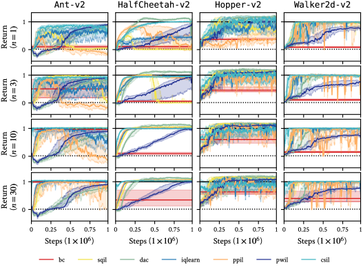
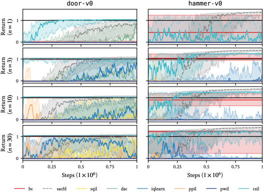
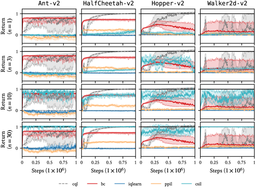
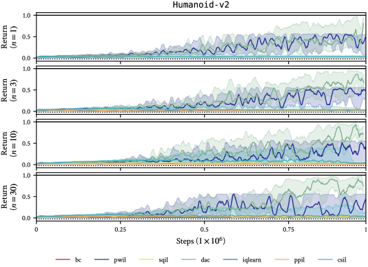
M.2 Continuous control from agent demonstrations

Step-wise results.

Figure 28, 29 and 30 show step-wise performance curves, as opposed to the demonstration-wise results in the main paper. For online experiments, steps refers to the actor and learner, while for offline experiments, steps correspond to the learner.

Humanoid-v2 results.

We evaluated csil and baselines on the high-dimensional Humanoid-v2 locomotion task in Figure 31. We found that csil struggled to solve this task due to the difficulty for bc to perform well at this task, even when using all 200 of the available demonstrations in the dataset.

One aspect of Humanoid-v2 to note is that a return of around $5000$ (around 0.5 normalized) corresponds to the survival / standing bonus, rather than actual locomotion (around 9000). While the positive nature of the coherent reward enabled learning the stabilize, this was not consistent across seeds. We also found it difficult to reproduce baseline results due to iqlearn’s instability, which we also reproduced on the author’s implementation [Div99, 2021]. In theory, bc should be able to approximate the original optimal agent’s policy with sufficient demonstrations. We believe the solution may be additional bc regularization, as the environment has a 376-dimensional state space.

Performance improvement of coherent imitation learning

A desired quality of csil is its ability to match or exceed its initial bc policy. Figures 32, 33 and 34 show the performance of csil relative to its initial bc policy. Empirical, csil matches or exceeds the initial bc policy across environments.

Figure 32: Normalized performance of csil for online Gym tasks against its bc initialization. Uncertainty intervals depict quartiles over ten seeds. $n$ refers to demonstration trajectories.

Figure 33: Normalized performance of csil for online Adroit tasks against its bc initialization. Uncertainty intervals depict quartiles over ten seeds. $n$ refers to demonstration trajectories.

Figure 34: Normalized performance of csil for offline Gym tasks against its bc initialization. Uncertainty intervals depict quartiles over ten seeds. $n$ refers to demonstration trajectories.

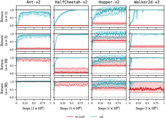
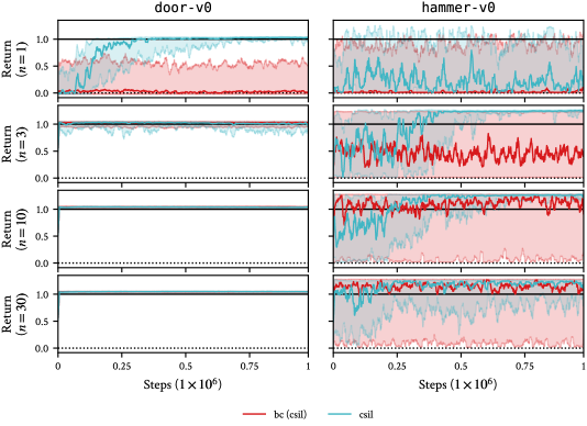
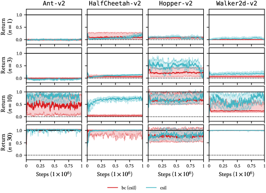
Divergence in minimax soft imitation learning

To investigate the performance issues in iqlearn and ppil relative to csil, we monitor a few key diagnostics during training for online door-v0 and offline Ant-v2 in Figure 35. One key observation is the drift in the bc accuracy. We attribute this to the instability in the reward or critic due to the saddle-point optimization.

Figure 35: We investigate the weakness of iqlearn and ppil for offline learning (Ant-v2) and high-dimensional action spaces (door-v0). Compared to csil, iqlearn and ppil have less stable and effective $Q$ values, in particular for the expert demonstrations, which results in the policy not inaccurately predicting the demonstration actions (expert_mse).

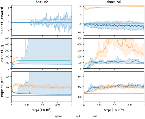
M.3 Continuous control from human demonstrations

Figure 36 shows performance on the online setting w.r.t. learning steps, and Figure 37 shows the offline performance w.r.t. learning steps. For online learning, csil is consistently more sample efficient than the oracle baseline sacfd, presumably due to bc pre-training and csil’s shaped reward w.r.t. robomimic’s sparse reward on success. csil was also able to surpass Mandlekar et al. [2021]’s success rate on NutAssemblySquare. For offline learning from suboptimal human demonstrations, it appears to be a much harder setting for csil to improve on the initial bc policy, especially for harder tasks.

Figure 36: Average success rate over 50 evaluations for online imitation learning for robomimic tasks. Uncertainty intervals depict quartiles over ten seeds. The bc policy is trained on the demonstration data. $n$ refers to demonstration trajectories.

Figure 37: Average success rate over 50 evaluations for offline imitation learning for robomimic tasks. Uncertainty intervals depict quartiles over ten seeds. This experiment shows that learning from suboptimal offline demonstrations is much harder than on-policy data. It is also harder to use the KL regularization to ensure improvement over the initial policy. $n$ refers to demonstration trajectories.

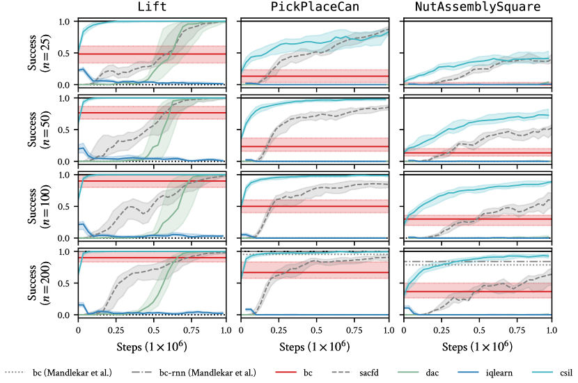
Appendix N Ablation studies

This section includes ablation studies for the csil algorithm and baselines.

N.1 Baselines with behavioral cloning pre-training

To assess the importance of bc pre-training, we evaluate the performance of iqlearn and ppil with bc pre-training in Figure 38. While difficult to see across all experiments, there is a small drop in performance at the beginning of training as the policy ‘unlearns’ as the critic and reward are randomly initialized since there is no notion of coherency.

Figure 38: Normalized performance of iqlearn and ppil for online Gym tasks with bc pre-training. Uncertainty intervals depict quartiles over ten seeds. $n$ refers to demonstration trajectories.

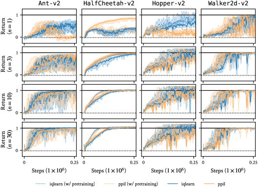
N.2 Baselines with behavioral cloning pre-training and KL regularization

To bring iqlearn and ppil closer to csil, we implement the baselines with bc pre-training and kl regularization, but with sac-style policies rather than hetstat. We evaluate on the harder tasks, online Adroit, and offline Gym, to see if these features contribute sufficient stability to solve the task. Both Figure 39 and Figure 40 show an increase in initial performance, it is not enough to completely stabilize the algorithms.

Figure 39: Normalized performance of iqlearn and ppil for online Adroit tasks with bc pre-training. Uncertainty intervals depict quartiles over ten seeds. $n$ refers to demonstration trajectories.

Figure 40: Normalized performance of iqlearn and ppil for offline Gym tasks with bc pre-training. Uncertainty intervals depict quartiles over ten seeds. $n$ refers to demonstration trajectories.

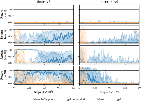
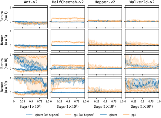
N.3 Baselines with heteroscedastic stationary policies

To investigate the impact of hetstat policies alone, we evaluated ppil and iqlearn with hetstat policies on the online Gym tasks in Figure 41. There is not a significant discrepancy between mlp and hetstat policies.

Figure 41: Normalized performance of iqlearn and ppil for online Gym tasks with hetstat policies. Uncertainty intervals depict quartiles over ten seeds. $n$ refers to demonstration trajectories.

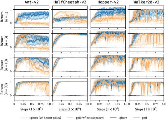
N.4 Baselines with pre-trained heteroscedastic stationary policies as priors

To bring iqlearn and ppil closer to csil, we implement the baselines with bc pre-training, hetstat policies and kl regularization with stationary policies. We evaluate on the harder tasks, online Adroit and offline Gym, to see if these features contribute sufficient stability to solve the task. Both Figure 42 and Figure 43 show an increase in performance, especially with increasing number of demonstrations, but it is ultimately not enough to completely stabilize the algorithms to the degree seen in csil.

Figure 42: Normalized performance of iqlearn and ppil for online Adroit tasks with pre-trained hetstat policies and kl-regularization. Uncertainty intervals depict quartiles over ten seeds. $n$ refers to demonstration trajectories.

Figure 43: Normalized performance of iqlearn and ppil for offline Gym tasks with pre-trained hetstat policies and kl-regularization. Uncertainty intervals depict quartiles over ten seeds. $n$ refers to demonstration trajectories.

Figure 44: Normalized performance of csil for online Gym tasks a critic pre-training ablation. Uncertainty intervals depict quartiles over ten seeds. $n$ refers to demonstration trajectories.

Figure 45: Normalized performance of csil for online Gym tasks with a reward finetuning ablation. Uncertainty intervals depict quartiles over ten seeds. Refinement is most important in the low demonstration setting where the initial bc policy and coherent reward is less defined, and therefore the initial policy is poor and the coherent reward is more susceptible to exploitation of the stationary approximation errors. $n$ refers to demonstration trajectories.

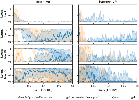
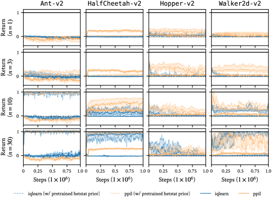
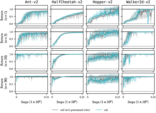
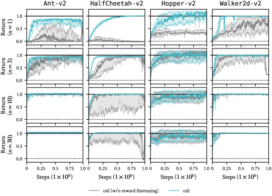
N.5 Importance of critic pre-training

To ablate the importance of critic pre-training, Figure 44 shows the performance difference on online Gym tasks. Critic pre-training provides only a minor performance improvement.

N.6 Importance of reward finetuning

To ablate the importance of reward finetuning, Figure 45. shows the performance difference on online Gym tasks. Reward finetuning is crucial in the setting of few demonstration trajectories, as the imitation reward is sparse and therefore csil is more susceptible to approximation errors in stationarity. It is also important for reducing performance variance and ensuring stable convergence.

N.7 Importance of critic regularization

To ablate the importance of critic Jacobian regularization, Figure 46. shows the performance difference on online Gym tasks. The regularization has several benefits. One is faster convergence, as it encodes the coherency inductive bias into the critic. A second is stability, as it encodes first-order optimality w.r.t. the expert demonstrations, mitigating errors in policy evaluation. The inductive bias also appears to reduce performance variance. One observation is that the performance of Ant-v2 improves without the regularization. This difference could be because the regularization encourages imitation rather than apprenticeship-style learning where the agent improves on the expert.

N.8 Stationary and non-stationary policies

One important ablation for csil is evaluating the performance with standard mlp policies like those used by the baselines. We found that this setting was not numerically stable enough to complete an ablation experiment. Due to the spurious behavior (e.g., as shown in Figure 3), the log-likelihood values used in the reward varied significantly in magnitude, destabilizing learning significantly, leading to policies that could no longer be numerically evaluated. This result means that stationarity is a critical component of csil.

N.9 Effectiveness of constant rewards

Many imitation rewards typically encode an inductive bias of positivity or negativity, which encourage survival or ‘minimum time’ strategies respectively [Kostrikov et al., 2019]. We ablate csil with this inductive bias for survival tasks (Hopper-v2 and Walker-v2) and minimum-time tasks (robomimic). Figure 47 shows that positive-only rewards are sufficient for Hopper-v2 but not for Walker-v2. Figure 48 shows that negative-only rewards is effective for the simpler tasks (Lift) but not the harder tasks (NutAssemblySquare).

N.10 Importance of behavioral cloning pre-training

Figure 49 shows csil without any policy pre-training, so the reward is learned only though the finetuning objective. csil without pre-training does not appear to work for any of the tasks. This poor performance could be attributed to the lack of hyperparameter tuning, since the reward learning hyperparameters were chosen assuming a good initialization. It could also due to the maximum likelihood fitting of the coherent reward, since the refinement does not use the ‘faithful’ objective (Section D) that improves the regression fit.

Figure 46: Normalized performance of csil for online MuJoCo Gym without regularizing the critic Jacobian. Uncertainty intervals depict quartiles over ten seeds. The benefit of this regularization is somewhat environment dependent, but clearly regularizes learning to the demonstrations effectively in many cases. Performance reduction is likely due to underfiftting during policy evaluation due to the regularization. $n$ refers to demonstration trajectories.

Figure 47: Online MuJoCo Gym tasks with absorbing states where csil is given a constant +1 reward function. Uncertainty intervals depict quartiles over ten seeds. While this is sometimes enough to solve the task (due to the absorbing state), the csil reward performs equal or better. $n$ refers to demonstration trajectories.

Figure 48: Online robomimic tasks where csil is given a constant -1 reward function. Uncertainty intervals depict quartiles over ten seeds. While a constant reward is sometimes enough to solve the task (due to the absorbing state), the csil reward performs roughly equal or better, with lower performance variance. $n$ refers to demonstration trajectories.

Figure 49: Online MuJoCo gym tasks where csil has no bc pre-training. Uncertainty intervals depict quartiles over 5 seeds. $n$ refers to demonstration trajectories.

References

- Osa et al. [2018] Takayuki Osa, Joni Pajarinen, Gerhard Neumann, J Andrew Bagnell, Pieter Abbeel, Jan Peters, et al. An algorithmic perspective on imitation learning. Foundations and Trends® in Robotics, 2018.
- Schaal [1999] Stefan Schaal. Is imitation learning the route to humanoid robots? Trends in Cognitive Sciences, 1999.
- Pomerleau [1991] D. A. Pomerleau. Efficient training of artificial neural networks for autonomous navigation. Neural Computation, 1991.
- Kalman [1964] Rudolph E. Kalman. When is a linear control system optimal? Journal of Basic Engineering, 1964.
- Ng and Russell [2000] Andrew Y. Ng and Stuart J. Russell. Algorithms for inverse reinforcement learning. In International Conference on Machine Learning, 2000.
- Abbeel and Ng [2004] P. Abbeel and A. Y. Ng. Apprenticeship learning via inverse reinforcement learning. In International Conference on Machine Learning, 2004.
- Puterman [2014] Martin L Puterman. Markov Decision Processes: Discrete Stochastic Dynamic Programming. John Wiley & Sons, 2014.
- Sutton and Barto [2018] Richard S Sutton and Andrew G Barto. Reinforcement learning: An introduction. MIT press, 2018.
- Ross and Bagnell [2011] Stéphane Ross and Drew Bagnell. A reduction of imitation learning and structured prediction to no-regret online learning. In International Conference on Artificial Intelligence and Statistics, 2011.
- Zheng et al. [2022] Boyuan Zheng, Sunny Verma, Jianlong Zhou, Ivor W Tsang, and Fang Chen. Imitation learning: Progress, taxonomies and challenges. IEEE Transactions on Neural Networks and Learning Systems, 2022.
- Orsini et al. [2021] Manu Orsini, Anton Raichuk, Léonard Hussenot, Damien Vincent, Robert Dadashi, Sertan Girgin, Matthieu Geist, Olivier Bachem, Olivier Pietquin, and Marcin Andrychowicz. What matters for adversarial imitation learning? In Advances in Neural Information Processing Systems, 2021.
- Jena et al. [2020] Rohit Jena, Changliu Liu, and Katia Sycara. Augmenting GAIL with BC for sample efficient imitation learning. In Conference on Robot Learning, 2020.
- Peters et al. [2010] Jan Peters, Katharina Mülling, and Yasemin Altün. Relative entropy policy search. In Proceedings of the AAAI Conference on Artificial Intelligence, 2010.
- Fox et al. [2016] Roy Fox, Ari Pakman, and Naftali Tishby. Taming the noise in reinforcement learning via soft updates. In Conference on Uncertainty in Artificial Intelligence, 2016.
- Van Hoof et al. [2017] Herke Van Hoof, Gerhard Neumann, and Jan Peters. Non-parametric policy search with limited information loss. Journal of Machine Learning Research, 2017.
- Abdolmaleki et al. [2018] Abbas Abdolmaleki, Jost Tobias Springenberg, Yuval Tassa, Remi Munos, Nicolas Heess, and Martin Riedmiller. Maximum a Posteriori policy optimisation. In International Conference on Learning Representations, 2018.
- Haarnoja et al. [2018] Tuomas Haarnoja, Aurick Zhou, Pieter Abbeel, and Sergey Levine. Soft actor-critic: Off-policy maximum entropy deep reinforcement learning with a stochastic actor. In International Conference on Machine Learning, 2018.
- Fellows et al. [2019] Matthew Fellows, Anuj Mahajan, Tim GJ Rudner, and Shimon Whiteson. VIREL: A variational inference framework for reinforcement learning. Advances in Neural Information Processing Systems, 2019.
- Bas-Serrano et al. [2021] Joan Bas-Serrano, Sebastian Curi, Andreas Krause, and Gergely Neu. Logistic -learning. In International Conference on Artificial Intelligence and Statistics, 2021.
- Pirotta and Restelli [2016] Matteo Pirotta and Marcello Restelli. Inverse reinforcement learning through policy gradient minimization. In Proceedings of the AAAI Conference on Artificial Intelligence, 2016.
- Ramponi et al. [2020] Giorgia Ramponi, Gianluca Drappo, and Marcello Restelli. Inverse reinforcement learning from a gradient-based learner. In Advances in Neural Information Processing Systems, 2020.
- Zhang et al. [2022] Yi-Feng Zhang, Fan-Ming Luo, and Yang Yu. Improve generated adversarial imitation learning with reward variance regularization. Machine Learning, 2022.
- Reddy et al. [2019] Siddharth Reddy, Anca D Dragan, and Sergey Levine. SQIL: Imitation learning via reinforcement learning with sparse rewards. In International Conference on Learning Representations, 2019.
- Brantley et al. [2020] Kiante Brantley, Wen Sun, and Mikael Henaff. Disagreement-regularized imitation learning. In International Conference on Learning Representations, 2020.
- Rajaraman et al. [2020] Nived Rajaraman, Lin Yang, Jiantao Jiao, and Kannan Ramchandran. Toward the fundamental limits of imitation learning. Advances in Neural Information Processing Systems, 2020.
- Russell [1998] Stuart Russell. Learning agents for uncertain environments. In Conference on Computational Learning Theory, 1998.
- Syed and Schapire [2007] Umar Syed and Robert E. Schapire. A game-theoretic approach to apprenticeship learning. In Advances in Neural Information Processing Systems, 2007.
- Syed et al. [2008] Umar Syed, M. Bowling, and R.E. Schapire. Apprenticeship learning using linear programming. In International Conference on Machine Learning, 2008.
- Xu et al. [2020] Tian Xu, Ziniu Li, and Yang Yu. Error bounds of imitating policies and environments. Advances in Neural Information Processing Systems, 2020.
- Ziebart [2010] Brian D Ziebart. Modeling purposeful adaptive behavior with the principle of maximum causal entropy. Carnegie Mellon University, 2010.
- Jaynes [1982] Edwin T Jaynes. On the rationale of maximum-entropy methods. Proceedings of the IEEE, 1982.
- Marino et al. [2021] Joseph Marino, Alexandre Piché, Alessandro Davide Ialongo, and Yisong Yue. Iterative amortized policy optimization. In Advances in Neural Information Processing Systems, 2021.
- Barber [2012] David Barber. Bayesian reasoning and machine learning. Cambridge University Press, 2012.
- Rawlik et al. [2013] Konrad Rawlik, Marc Toussaint, and Sethu Vijayakumar. On stochastic optimal control and reinforcement learning by approximate inference. In Robotics: Science and Systems, 2013.
- Watson and Peters [2022] Joe Watson and Jan Peters. Inferring smooth control: Monte Carlo posterior policy iteration with Gaussian processes. In Conference on Robot Learning, 2022.
- Metelli et al. [2017] Alberto Maria Metelli, Matteo Pirotta, and Marcello Restelli. Compatible reward inverse reinforcement learning. In Advances in Neural Information Processing Systems, 2017.
- Ho and Ermon [2016] Jonathon Ho and Stefan Ermon. Generative adversarial imitation learning. In Advances in Neural Information Processing Systems, 2016.
- Fu et al. [2018a] Justin Fu, Katie Luo, and Sergey Levine. Learning robust rewards with adverserial inverse reinforcement learning. In International Conference on Learning Representations, 2018a.
- Ghasemipour et al. [2019] Seyed Kamyar Seyed Ghasemipour, Richard Zemel, and Shixiang Gu. A divergence minimization perspective on imitation learning methods. In Conference on Robot Learning, 2019.
- Kostrikov et al. [2019] Ilya Kostrikov, Kumar Krishna Agrawal, Debidatta Dwibedi, Sergey Levine, and Jonathan Tompson. Discriminator-actor-critic: Addressing sample inefficiency and reward bias in adversarial imitation learning. In International Conference on Learning Representations, 2019.
- Kostrikov et al. [2020] Ilya Kostrikov, Ofir Nachum, and Jonathan Tompson. Imitation learning via off-policy distribution matching. In International Conference on Learning Representations, 2020.
- Garg et al. [2021] Divyansh Garg, Shuvam Chakraborty, Chris Cundy, Jiaming Song, and Stefano Ermon. IQ-learn: Inverse soft- learning for imitation. In Advances in Neural Information Processing Systems, 2021.
- Viano et al. [2022] Luca Viano, Angeliki Kamoutsi, Gergely Neu, Igor Krawczuk, and Volkan Cevher. Proximal point imitation learning. In Advances in Neural Information Processing Systems, 2022.
- Dadashi et al. [2021] Robert Dadashi, Leonard Hussenot, Matthieu Geist, and Olivier Pietquin. Primal Wasserstein imitation learning. In International Conference on Learning Representations, 2021.
- Boularias et al. [2011] Abdeslam Boularias, Jens Kober, and Jan Peters. Relative entropy inverse reinforcement learning. In International Conference on Artificial Intelligence and Statistics, 2011.
- Wulfmeier et al. [2015] Markus Wulfmeier, Peter Ondruska, and Ingmar Posner. Maximum entropy deep inverse reinforcement learning. arXiv preprint arXiv:1507.04888, 2015.
- Arenz et al. [2016] Oleg Arenz, Hany Abdulsamad, and Gerhard Neumann. Optimal control and inverse optimal control by distribution matching. In IEEE/RSJ International Conference on Intelligent Robots and Systems, 2016.
- Finn et al. [2016] Chelsea Finn, Sergey Levine, and Pieter Abbeel. Guided cost learning: Deep inverse optimal control via policy optimization. In International Conference on Machine Learning, 2016.
- Ni et al. [2020] Tianwei Ni, Harshit Sikchi, Yufei Wang, Tejus Gupta, Lisa Lee, and Ben Eysenbach. -IRL: Inverse reinforcement learning via state marginal matching. In Conference on Robot Learning, 2020.
- Neu and Szepesvári [2007] Gergeley Neu and Csaba Szepesvári. Apprenticeship learning using inverse reinforcement learning and gradient methods. In Conference on Uncertainty in Artificial Intelligence, 2007.
- Barde et al. [2020] Paul Barde, Julien Roy, Wonseok Jeon, Joelle Pineau, Chris Pal, and Derek Nowrouzezahrai. Adversarial soft advantage fitting: Imitation learning without policy optimization. In Advances in Neural Information Processing Systems, 2020.
- Xu et al. [2022] Haoran Xu, Xianyuan Zhan, Honglei Yin, and Huiling Qin. Discriminator-weighted offline imitation learning from suboptimal demonstrations. In International Conference on Machine Learning, 2022.
- Jacq et al. [2019] Alexis Jacq, Matthieu Geist, Ana Paiva, and Olivier Pietquin. Learning from a learner. In International Conference on Machine Learning, 2019.
- Cao et al. [2021] Haoyang Cao, Samuel Cohen, and Lukasz Szpruch. Identifiability in inverse reinforcement learning. In Advances in Neural Information Processing Systems, 2021.
- Ng et al. [1999] Andrew Y. Ng, Daishi Harada, and Stuart J. Russell. Policy invariance under reward transformations: Theory and application to reward shaping. In International Conference on Machine Learning, 1999.
- van Campenhout and Cover [1981] Jan van Campenhout and Thomas Cover. Maximum entropy and conditional probability. IEEE Transactions on Information Theory, 1981.
- Guedj [2019] Benjamin Guedj. A primer on PAC-Bayesian learning. In Proceedings of the second congress of the French Mathematical Society, 2019.
- Alquier et al. [2016] Pierre Alquier, James Ridgway, and Nicolas Chopin. On the properties of variational approximations of Gibbs posteriors. Journal of Machine Learning Research, 2016.
- Knoblauch et al. [2022] Jeremias Knoblauch, Jack Jewson, and Theodoros Damoulas. An optimization-centric view on Bayes’ rule: Reviewing and generalizing variational inference. Journal of Machine Learning Research, 2022.
- Oh et al. [2023] Hanbit Oh, Hikaru Sasaki, Brendan Michael, and Takamitsu Matsubara. Bayesian disturbance injection: Robust imitation learning of flexible policies for robot manipulation. Neural Networks, 2023.
- Rudner et al. [2021] Tim GJ Rudner, Cong Lu, Michael A Osborne, Yarin Gal, and Yee Teh. On pathologies in KL-regularized reinforcement learning from expert demonstrations. Advances in Neural Information Processing Systems, 2021.
- Rasmussen and Williams [2006] Carl E. Rasmussen and Chris Williams. Gaussian Processes for Machine Learning. MIT Press, 2006.
- Le et al. [2005] Quoc V. Le, Alex J. Smola, and Stéphane Canu. Heteroscedastic Gaussian process regression. In International Conference on Machine Learning, 2005.
- Jankowiak et al. [2020] Martin Jankowiak, Geoff Pleiss, and Jacob Gardner. Parametric Gaussian process regressors. In International Conference on Machine Learning, 2020.
- Fu et al. [2018b] Justin Fu, Katie Luo, and Sergey Levine. Learning robust rewards with adverserial inverse reinforcement learning. In International Conference on Learning Representations, 2018b.
- Geist et al. [2019] Matthieu Geist, Bruno Scherrer, and Olivier Pietquin. A theory of regularized Markov decision processes. In International Conference on Machine Learning, 2019.
- Cox and Miller [1977] David Roxbee Cox and Hilton David Miller. The theory of stochastic processes. CRC press, 1977.
- Meronen et al. [2021] Lassi Meronen, Martin Trapp, and Arno Solin. Periodic activation functions induce stationarity. In Advances in Neural Information Processing Systems, 2021.
- Siegel et al. [2020] Noah Siegel, Jost Tobias Springenberg, Felix Berkenkamp, Abbas Abdolmaleki, Michael Neunert, Thomas Lampe, Roland Hafner, Nicolas Heess, and Martin Riedmiller. Keep doing what worked: Behavior modelling priors for offline reinforcement learning. In International Conference on Learning Representations, 2020.
- Seitzer et al. [2022] Maximilian Seitzer, Arash Tavakoli, Dimitrije Antic, and Georg Martius. On the pitfalls of heteroscedastic uncertainty estimation with probabilistic neural networks. In International Conference on Learning Representations, 2022.
- Stirn et al. [2023] Andrew Stirn, Hans-Hermann Wessels, Megan Schertzer, Laura Pereira, Neville E. Sanjana, and David A. Knowles. Faithful heteroscedastic regression with neural networks. In International Conference on Artificial Intelligence and Statistics, 2023.
- Todorov et al. [2012] Emanuel Todorov, Tom Erez, and Yuval Tassa. MuJoCo: A physics engine for model-based control. In IEEE International Conference on Intelligent Robots and Systems, 2012.
- Brockman et al. [2016] Greg Brockman, Vicki Cheung, Ludwig Pettersson, Jonas Schneider, John Schulman, Jie Tang, and Wojciech Zaremba. OpenAI Gym. arXiv preprint arXiv:1606.01540, 2016.
- Rajeswaran et al. [2018] Aravind Rajeswaran, Vikash Kumar, Abhishek Gupta, Giulia Vezzani, John Schulman, Emanuel Todorov, and Sergey Levine. Learning complex dexterous manipulation with deep reinforcement learning and demonstrations. In Robotics: Science and Systems, 2018.
- Fu et al. [2020] Justin Fu, Aviral Kumar, Ofir Nachum, George Tucker, and Sergey Levine. D4rl: Datasets for deep data-driven reinforcement learning. arXiv preprint arXiv:2004.07219, 2020.
- Hoffman et al. [2020] Matthew W Hoffman, Bobak Shahriari, John Aslanides, Gabriel Barth-Maron, Nikola Momchev, Danila Sinopalnikov, Piotr Stańczyk, Sabela Ramos, Anton Raichuk, Damien Vincent, et al. Acme: A research framework for distributed reinforcement learning. arXiv preprint arXiv:2006.00979, 2020.
- Ramos et al. [2021] Sabela Ramos, Sertan Girgin, Léonard Hussenot, Damien Vincent, Hanna Yakubovich, Daniel Toyama, Anita Gergely, Piotr Stanczyk, Raphael Marinier, Jeremiah Harmsen, et al. Rlds: An ecosystem to generate, share and use datasets in reinforcement learning. arXiv preprint arXiv:2111.02767, 2021.
- Vecerik et al. [2017] Mel Vecerik, Todd Hester, Jonathan Scholz, Fumin Wang, Olivier Pietquin, Bilal Piot, Nicolas Heess, Thomas Rothörl, Thomas Lampe, and Martin Riedmiller. Leveraging demonstrations for deep reinforcement learning on robotics problems with sparse rewards. arXiv preprint arXiv:1707.08817, 2017.
- Arenz and Neumann [2020] Oleg Arenz and Gerhard Neumann. Non-adversarial imitation learning and its connections to adversarial methods. arxiv preprint arxiv:2008.03525, 2020.
- Ziniu et al. [2022] Li Ziniu, Xu Tian, Yu Yang, and Luo Zhi-Quan. Rethinking ValueDice – Does it really improve performance? ICLR Blog Track, https://iclr-blog-track.github.io/2022/03/25/rethinking-valuedice/, 2022.
- Kumar et al. [2020] Aviral Kumar, Aurick Zhou, George Tucker, and Sergey Levine. Conservative Q-learning for offline reinforcement learning. Advances in Neural Information Processing Systems, 2020.
- Ma et al. [2022] Yecheng Ma, Andrew Shen, Dinesh Jayaraman, and Osbert Bastani. Versatile offline imitation from observations and examples via regularized state-occupancy matching. In International Conference on Machine Learning, 2022.
- Kim et al. [2022] Geon-Hyeong Kim, Seokin Seo, Jongmin Lee, Wonseok Jeon, HyeongJoo Hwang, Hongseok Yang, and Kee-Eung Kim. DemoDICE: Offline imitation learning with supplementary imperfect demonstrations. In International Conference on Learning Representations, 2022.
- Mandlekar et al. [2021] Ajay Mandlekar, Danfei Xu, Josiah Wong, Soroush Nasiriany, Chen Wang, Rohun Kulkarni, Li Fei-Fei, Silvio Savarese, Yuke Zhu, and Roberto Martín-Martín. What matters in learning from offline human demonstrations for robot manipulation. In Conference on Robot Learning, 2021.
- Zołna et al. [2020] Konrad Zołna, Alexander Novikov, Ksenia Konyushkova, Caglar Gulcehre, Ziyu Wang, Yusuf Aytar, Misha Denil, Nando de Freitas, and Scott Reed. Offline learning from demonstrations and unlabeled experience. In Offline Reinforcement Learning Workshop, NeurIPS, 2020.
- Deisenroth et al. [2013] Marc Peter Deisenroth, Gerhard Neumann, and Jan Peters. A survey on policy search for robotics. Foundations and Trends in Robotics, 2013.
- Al-Hafez et al. [2023] Firas Al-Hafez, Davide Tateo, Oleg Arenz, Guoping Zhao, and Jan Peters. LS-IQ: Implicit reward regularization for inverse reinforcement learning. In International Conference on Learning Representations, 2023.
- Szot et al. [2023] Andrew Szot, Amy Zhang, Dhruv Batra, Zsolt Kira, and Franziska Meier. BC-IRL: Learning generalizable reward functions from demonstrations. In International Conference on Learning Representations, 2023.
- Taranovic et al. [2022] Aleksandar Taranovic, Andras Gabor Kupcsik, Niklas Freymuth, and Gerhard Neumann. Adversarial imitation learning with preferences. In International Conference on Learning Representations, 2022.
- Swamy et al. [2022] Gokul Swamy, Nived Rajaraman, Matt Peng, Sanjiban Choudhury, J Bagnell, Steven Z Wu, Jiantao Jiao, and Kannan Ramchandran. Minimax optimal online imitation learning via replay estimation. Advances in Neural Information Processing Systems, 2022.
- Sasaki and Yamashina [2021] Fumihiro Sasaki and Ryota Yamashina. Behavioral cloning from noisy demonstrations. In International Conference on Learning Representations, 2021.
- Ramachandran and Amir [2007] Deepak Ramachandran and Eyal Amir. Bayesian inverse reinforcement learning. In International Joint Conference on Artifical Intelligence, 2007.
- Choi and Kim [2011] Jaedeug Choi and Kee-Eung Kim. MAP inference for Bayesian inverse reinforcement learning. Advances in Neural Information Processing Systems, 2011.
- Da Prato and Zabczyk [2014] Giuseppe Da Prato and Jerzy Zabczyk. Stochastic equations in infinite dimensions. Cambridge University Press, 2014.
- Chatfield [1989] Chris Chatfield. The analysis of time series: An introduction. Chapman and Hall, 1989.
- Liu et al. [2020] Jeremiah Liu, Zi Lin, Shreyas Padhy, Dustin Tran, Tania Bedrax Weiss, and Balaji Lakshminarayanan. Simple and principled uncertainty estimation with deterministic deep learning via distance awareness. In Advances in Neural Information Processing Systems, 2020.
- Schulman [2020] John Schulman. Approximating KL divergence. http://joschu.net/blog/kl-approx.html, 2020.
- Sun et al. [2019] Shengyang Sun, Guodong Zhang, Jiaxin Shi, and Roger Grosse. Functional variational Bayesian neural networks. In International Conference on Learning Representations, 2019.
- Watson et al. [2021] Joe Watson, Jihao Andreas Lin, Pascal Klink, and Jan Peters. Neural linear models with functional Gaussian process priors. In Third Symposium on Advances in Approximate Bayesian Inference, 2021.
- Div99 [2021] Div99. IQ-Learn implementation. https://github.com/Div99/IQ-Learn, 2021.
- Wu [2016] Yihong Wu. Lecture notes for ECE598YW: Information-theoretic methods in high-dimensional statistics. Yale University, 2016.
- Bradbury et al. [2018] James Bradbury, Roy Frostig, Peter Hawkins, Matthew James Johnson, Chris Leary, Dougal Maclaurin, George Necula, Adam Paszke, Jake VanderPlas, Skye Wanderman-Milne, and Qiao Zhang. JAX: Composable transformations of Python+NumPy programs, 2018. URL http://github.com/google/jax.
- Babuschkin et al. [2020] Igor Babuschkin, Kate Baumli, Alison Bell, Surya Bhupatiraju, Jake Bruce, Peter Buchlovsky, David Budden, Trevor Cai, Aidan Clark, Ivo Danihelka, Antoine Dedieu, Claudio Fantacci, Jonathan Godwin, Chris Jones, Ross Hemsley, Tom Hennigan, Matteo Hessel, Shaobo Hou, Steven Kapturowski, Thomas Keck, Iurii Kemaev, Michael King, Markus Kunesch, Lena Martens, Hamza Merzic, Vladimir Mikulik, Tamara Norman, George Papamakarios, John Quan, Roman Ring, Francisco Ruiz, Alvaro Sanchez, Laurent Sartran, Rosalia Schneider, Eren Sezener, Stephen Spencer, Srivatsan Srinivasan, Miloš Stanojević, Wojciech Stokowiec, Luyu Wang, Guangyao Zhou, and Fabio Viola. The DeepMind JAX Ecosystem, 2020. URL http://github.com/deepmind.
- lviano [2022] lviano. Proximal point imitation learning implementation. https://github.com/lviano/p2il, 2022.
- geon-hyeong [2022] geon-hyeong. DemoDICE implementation. https://github.com/geon-hyeong/imitation-dice, 2022.
- JasonMa2016 [2022] JasonMa2016. SMODICE implementation. https://github.com/JasonMa2016/SMODICE, 2022.
- Espeholt et al. [2018] Lasse Espeholt, Hubert Soyer, Remi Munos, Karen Simonyan, Vlad Mnih, Tom Ward, Yotam Doron, Vlad Firoiu, Tim Harley, Iain Dunning, et al. Impala: Scalable distributed deep-RL with importance weighted actor-learner architectures. In International conference on machine learning, 2018.