Flexible Variable Selection for Clustering and Classification

Abstract

The importance of variable selection for clustering has been recognized for some time, and mixture models are well-established as a statistical approach to clustering. Yet, the literature on variable selection in model-based clustering remains largely rooted in the assumption of Gaussian clusters. Unsurprisingly, variable selection algorithms based on this assumption tend to break down in the presence of cluster skewness. A novel variable selection algorithm is presented that utilizes the Manly transformation mixture model to select variables based on their ability to separate clusters, and is effective even when clusters depart from the Gaussian assumption. The proposed approach, which is implemented within the R package vscc, is compared to existing variable selection methods — including an existing method that can account for cluster skewness — using simulated and real datasets.

Keywords: Clustering; mixture models; variable selection; model-based clustering; skewness.

1 Introduction

Variable selection refers to the process by which informative variables are retained and uninformative variables are removed. Eliminating uninformative variables can improve both model fitting and model interpretability. As such, much research has been conducted on variable selection across statistical domains. One such domain is that of model-based clustering and classification — in this context, a variable is informative or not depending on whether it is useful for classification or clustering. The need for dimension reduction is evident for clustering and classification problems as noisy data can hide key features, such as groupings. A popular school of thought is that dimension reduction should happen in tandem with data clustering rather than before clustering (Steinley and Brusco, 2011; Bouveyron and Brunet-Saumard, 2014; McNicholas, 2016b). As such, variable selection methods that are embedded into clustering and classification algorithms are essential. Many such algorithms exist for Gaussian clustering algorithms; however, the same cannot be said for skewed clustering methods.

In this paper, we study the effect that skewness has on existing variable selection algorithms for classification and clustering and introduce a skewed analogue of the variable selection method VSCC (Andrews and McNicholas, 2014). Implementations of the original VSCC method and the extension introduced herein are available in the vscc package (Andrews et al., 2023) for R (R Core Team, 2023). This extension of VSCC is compared to a skewed extension of the clustvarsel algorithm (Raftery and Dean, 2006; Maugis et al., 2009; Scrucca and Raftery, 2018) called skewvarsel (Wallace et al., 2018), using both real data and simulated data.

2 Background

2.1 Finite Mixture Models

Finite mixture models arise from the assumption that a population contains sub-populations that can be modelled by a finite number of densities. Thus, these models lend themselves to clustering and classification problems. A random vector $\mathbf{X}$ belongs to finite mixture model if the density can be written

$$f(\mathbf{x}|\boldsymbol{\vartheta})=\sum_{g=1}^{G}\pi_{g}f_{g}(\mathbf{x}|\boldsymbol{\theta}_{g}),$$

where $\pi_{g}>0$ are the mixing proportions such that $\sum_{g=1}^{G}\pi_{g}=1$ and $f_{g}(\mathbf{x}|\boldsymbol{\theta}_{g})$ are the component densities. Most commonly, these component densities are taken to be multivariate Gaussian corresponding to the following component densities:

$$f(\mathbf{x}|\boldsymbol{\mu}_{g},\boldsymbol{\Sigma}_{g})=\sum_{g=1}^{G}\frac{\pi_{g}}{(2\pi)^{p/2}|\boldsymbol{\Sigma}_{g}|^{1/2}}\exp\left\{-\frac{1}{2}(\mathbf{x}-\boldsymbol{\mu}_{g})^{\top}\boldsymbol{\Sigma}_{g}^{-1}(\mathbf{x}-\boldsymbol{\mu}_{g})\right\},$$

where $\boldsymbol{\mu}_{g}$ denotes the mean and $\boldsymbol{\Sigma}_{g}$ is the covariance matrix for the $g$th component. However, in real applications it is uncommon for clusters to be Gaussian; in fact, clusters quite often cannot be well-represented by a Gaussian mixture (see Franczak et al., 2014; McNicholas, 2016a, for discussion). Thus, various asymmetric mixture models have been developed to aid in clustering and classification when skewness is present (see Section 2.2).

2.2 Skewed Mixture Models

There are two schools of thought when it comes to dealing with skewness. The first accounts for skewness directly with the use of flexible, asymmetric distributions. These include skew-symmetric distributions such as the skew-normal with density (Pyne et al., 2009):

$$f(\mathbf{y}|\boldsymbol{\mu},\boldsymbol{\Sigma},\boldsymbol{\delta})=2\phi_{p}(\mathbf{y}|\boldsymbol{\mu},\boldsymbol{\Sigma})\Phi_{1}(\boldsymbol{\delta}^{\top}\boldsymbol{\Sigma}^{-1}(\mathbf{y}-\boldsymbol{\mu});\boldsymbol{0},\boldsymbol{1}-\boldsymbol{\delta}^{\top}\boldsymbol{\Sigma}^{-1}\boldsymbol{\delta}),$$

where $\phi_{p}$ and $\Phi_{p}$ are the pdf and cdf, respectively, of the multivariate Gaussian distribution; $\boldsymbol{\Sigma}$ is the covariance matrix; $\boldsymbol{\delta}$ is the vector of skewness parameters; and $\boldsymbol{\mu}$ is the location parameter vector. Other common asymmetric distributions include the generalized hyperbolic distribution (Browne and McNicholas, 2015) and special and/or limiting cases thereof such as the normal inverse Gaussian (Karlis and Santourian, 2009), variance-gamma (McNicholas et al., 2017), and shifted asymmetric Laplace (Franczak et al., 2014) distributions. These distributions are examples of normal variance-mean mixtures. A $p$-dimensional random vector $\mathbf{X}$ is a normal variance-mean mixture if its density can be written as

$$f(\mathbf{x}|\boldsymbol{\mu},\boldsymbol{\Sigma},\boldsymbol{\alpha},\boldsymbol{\theta})=\int_{0}^{\infty}\phi_{p}(\mathbf{x}|\boldsymbol{\mu}+y\boldsymbol{\alpha},y\boldsymbol{\Sigma})h(y|\boldsymbol{\theta})dy,$$

where $\phi_{p}(\mathbf{x}|\boldsymbol{\mu}+y\boldsymbol{\alpha},y\boldsymbol{\Sigma})$ is the density of a $p$-dimensional multivariate normal distribution with mean $\boldsymbol{\mu}+y\boldsymbol{\alpha}$ and covariance $y\boldsymbol{\Sigma}$ and $h(y|\boldsymbol{\theta})$ is a density function for an asymmetric random variable $Y>0$ (Barndorff-Nielsen et al., 1982). In Section  5, we generate data from a mixture of multivariate variance-gamma distributions to compare variable selection methods in the presence of skewness. Data from a multivariate variance-gamma distribution can be generated via

$$\mathbf{X}=\boldsymbol{\mu}+Y\boldsymbol{\alpha}+\sqrt{Y}\mathbf{U},$$

where $Y\sim\text{gamma}(\lambda,\psi/2)$ and $\mathbf{U}\sim N_{p}(0,\boldsymbol{\Sigma})$ to result in $\mathbf{X}\sim V_{p}(\lambda,\psi,\boldsymbol{\mu},\boldsymbol{\Sigma},\boldsymbol{\alpha})$ (McNicholas et al., 2017).

The other school of thought for dealing with skewness utilizes transformations to near-normality. Two transformation mixture models exist: the first is a t-mixture model with a Box-Cox transformation (Lo and Gottardo, 2012). This model, however, would suffer from the shortcomings of the Box-Cox transformation, primarily its inability to handle left skew (Box and Cox, 1964). Additionally, the Box-Cox t-mixture assumes a global transformation parameter; accordingly, transformations do not vary by variables and components (Lo and Gottardo, 2012). The second transformation mixture model is a normal mixture model with a Manly transform (Zhu and Melnykov, 2018a). The Manly can handle both left and right skewed data, it can be applied to any real number, and it is given by

$$T(\mathbf{x}|\lambda)=\begin{cases}\frac{1}{\lambda}\left[\exp\{\lambda\mathbf{x}\}-1\right]&\text{if }\lambda\neq 0,\\ \mathbf{x}&\text{otherwise}.\end{cases}$$

By applying the back transform of the Manly, one will arrive at the following transformation-based density:

$$f_{T}(\mathbf{x}|\boldsymbol{\vartheta})=\phi(T(\mathbf{x}|\boldsymbol{\lambda})|\boldsymbol{\mu},\boldsymbol{\Sigma})J_{T}(\mathbf{x}|\boldsymbol{\lambda}).$$

where $\mathbf{x}$ is the original $p$-dimensional data vector, $\boldsymbol{\lambda}=(\lambda_{1},\lambda_{2},\ldots,\lambda_{p})^{\top}$ is the transformation vector, $\boldsymbol{\mu}$ is the location parameter vector, and $\boldsymbol{\Sigma}$ is the covariance matrix. The Jacobian of the back-transformation can be written

$$J_{T}(\mathbf{x}|\boldsymbol{\lambda})=\exp\{\boldsymbol{\lambda}^{\top}\mathbf{x}\},$$

and Zhu and Melnykov (2018a) used this back-transformation to obtain a skewed finite mixture model. This mixture model contains transformation parameters for each variable-cluster combination. As such, by incorporating the Manly into a model one must introduce ${G}{p}$ additional transformation parameters, potentially resulting in overparameterization. However, Zhu and Melnykov (2018a) recognized that it is unlikely for all variables to need to be transformed in all components. Therefore, to avoid over-parameterization, unnecessary transformation parameters are determined and zeroed out via a backwards or forwards selection process (Zhu and Melnykov, 2018a).

Forwards selection begins with a fully Gaussian mixture model (GMM). The GMM is then compared to ${G}{p}$ models each with one non-zero transformation parameter. The value of this non-zero transformation parameter is selected based on the simplex method, where the conditional expectation of the complete-data log-likelihood is maximized with respect to the skewness parameter in question. For each resulting model, the Bayesian information criterion (BIC; Schwarz, 1978) can be obtained via

$$\text{BIC}=2\log\hat{L}-p\log n,$$ (1)

where $\hat{L}$ is the maximized likelihood. Among the $Gp$ candidates, we select the model that maximizes the BIC. The algorithm continues until there are no further improvements to BIC, where parameters from the previous step are used as initializations in the next step.

Backwards selection begins with a fully skewed Manly mixture model. Iteratively, one transformation parameter is zeroed out and the BIC is obtained and compared. Again, this process is continued until no further improvements to BIC are obtained. Non-zero transition parameters are estimated via the Nelder-Mead algorithm, and remaining model parameters are estimated via an EM algorithm. We utilize the aforementioned work of Zhu and Melnykov (2018a) on the Manly mixture to extend the VSCC algorithm into the skewed space, this extension is detailed in Section 3.1. However, before doing so we must discuss properties of the Manly component densities that influence clustering results.

2.2.1 Invariance of the Manly Component Densities

The component Manly densities can be shown to be scale and shifting invariant, thus, operations performed to the data will not have an affect on the clustering results. A common pre-processing operation when clustering is to scale the data, thus such invariance is essential. Zhu and Melnykov (2018a) show that if $\mathbf{X}$ is distributed according to $f_{\mathbf{X}}(\mathbf{x};\boldsymbol{\mu},\boldsymbol{\Sigma},\boldsymbol{\lambda})=\phi(\mathcal{M}(\mathbf{x};\boldsymbol{\lambda});\boldsymbol{\mu},\boldsymbol{\Sigma})\exp\{\boldsymbol{\lambda}^{\top}\mathbf{x}\}$ and $\tilde{\mathbf{X}}=\mathbf{A}\mathbf{X}+\mathbf{h}$, where $\mathbf{A}$ is a diagonal scaling matrix and $\mathbf{h}$ is a shift vector, then

$$f_{\tilde{\mathbf{X}}}(\tilde{\mathbf{x}};\boldsymbol{\mu},\boldsymbol{\Sigma},\boldsymbol{\lambda},\mathbf{A},\mathbf{h})=f_{\mathbf{X}}(\tilde{\mathbf{x}};\tilde{\boldsymbol{\mu}},\tilde{\boldsymbol{\Sigma}},\tilde{\boldsymbol{\lambda}}).$$

This then proves invariance, and shows that the inclusion of parameters $\mathbf{A}$ and $\mathbf{h}$ leads to a non-identifiable model. This does not negate the following comments about identifiability.

2.2.2 Identifiability of the Manly component densities

A statistical model with parameter space $\Theta$ is identifiable if the following is true,

$$\mathcal{P}_{\theta_{1}}=\mathcal{P}_{\theta_{2}}\Rightarrow\theta_{1}=\theta_{2}\text{ for all }\theta_{1}\text{,}\theta_{2}\in\Theta.$$

Problems with mixture model identifiability regarding the label switching problem are well known and methods exist for handling said problem, such as requiring $\pi_{1}>\pi_{2}>\cdots>\pi_{G}$ (Redner and Walker, 1984; Stephens, 2000). Thus, the focus in terms of identifiability is focused on the component densities; in the case of the Manly component densities, it is easy to prove identifiability. This is a desirable quality; however, more recently focus has shifted from theoretical identifiability, as defined above, to empirical identifiability. Hennig (2023) defines empirical identifiability as the ability to find a consistent sequence of estimators. Due to the use of the Nelder-Mead algorithm (Nelder and Mead, 1965) for estimation of the transformation parameters, $\boldsymbol{\lambda}$, we are not able to discuss any consistency results. However, if we assume that the EM and the Nelder-Mead algorithms return maximum likelihood estimates - an assumption that is frequently made - then we can ensure consistency of the resulting estimators, thus ensuring empirical identifiability. That being said, results pertaining to both theoretical and empirical identifiability would be challenged in the presence of noisy and correlated variables, as discussed in Section 2.3.

2.3 Variable Selection

Herein we explore the effect noisy and correlated variables have on identifiability. Increasing correlation between variables has been shown to weaken identifiability (Koot et al., 2013). In the case where $\mathbf{X}_{1}\sim f_{X}(x;\boldsymbol{\vartheta})$ and $\mathbf{X}_{2}=\rho\mathbf{X}_{1}+(1-\rho)\mathbf{Z}$, where $\mathbf{Z}$ is some random noise and $\text{cov}(\mathbf{X}_{1},\mathbf{Z})=0$. The true covariance matrix of $(\mathbf{X}_{1},\mathbf{X}_{2})$ is

$$\boldsymbol{\Sigma}=\begin{bmatrix}\sigma_{1}^{2}&\rho\sigma_{1}^{2}\\ \rho\sigma_{1}^{2}&\rho^{2}\sigma_{1}^{2}+(1-\rho)^{2}\sigma_{Z}^{2}\end{bmatrix},$$

leading to non-identifiability. We can further show this with the Manly distribution where $T(\mathbf{X}|\boldsymbol{\lambda})\sim\mathcal{N}(\boldsymbol{\mu}_{x},\boldsymbol{\Sigma}_{x})$, $T(\mathbf{Z}|\boldsymbol{\lambda})\sim\mathcal{N}(\boldsymbol{\mu}_{z},\boldsymbol{\Sigma}_{z})$, and $\mathbf{Z},\mathbf{X}$ are independent. Then, the density of $\mathbf{X}+\mathbf{Z}$ is,

$$\frac{1}{(2\pi)^{p/2}|\boldsymbol{\Sigma}_{x}+\boldsymbol{\Sigma}_{z}|^{1/2}}\exp\left\{-\frac{1}{2}(\mathbf{x}-(\boldsymbol{\mu}_{x}+\boldsymbol{\mu}_{z}))^{\top}(\boldsymbol{\Sigma}_{x}+\boldsymbol{\Sigma}_{z})^{-1}(\mathbf{x}-(\boldsymbol{\mu}_{x}+\boldsymbol{\mu}_{z}))\right\}\exp\{\boldsymbol{\lambda}^{\top}(\mathbf{x}+\mathbf{z})\}.$$

Thus removing the identifiability property of the Manly component densities. This provides much motivation for variable selection as many real datasets are plagued with variables following such correlation schemes, see Section 4. Additionally, variables that are completed unrelated to the clustering structure are often captured, these variables would have a large effect on empirical identifiability of any mixture model, often resulting in an over-estimation of the number of components, as seen in Figure 2.

As such, the need for dimension reduction algorithms for model-based clustering is clear, this necessity is visualized in Figures 1 and 2, where we simulate data from a two-component, two-dimensional GMM and fit a GMM to this data before and after the addition of two noise variables. The first noise variable is random noise generated from a normal distribution, $\text{Noise}_{1}\sim N(4,2)$. The second noise variable is correlated to the second clustering variable via

$$\text{Noise}_{2}=0.8V2+0.2Z,$$

where $Z\sim N(0,5)$ and V2 is a clustering variable. We see that with the addition of just two noise variables, the clustering results begin to break down.

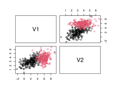
(a) True clusters from two-component GMM.

(b) Clustering results from GMM fit to simulated data in (a).

Figure 1: Clustering results from GMM on simulted data.

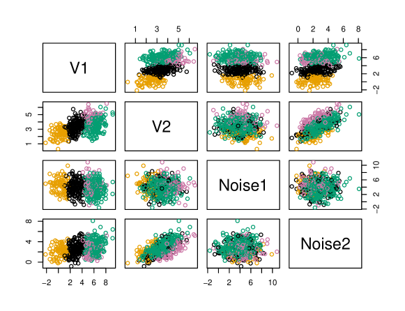
Figure 2: Clustering results from GMM fitted to simulated data in Figure 1(a) plus two noisy variables.

One type of dimension reduction method that could be used to overcome the poor clustering performance seen in Figure 2 is variable selection. Variable selection is the selection of important variables and the de-selection of unimportant variables — in the present context, important means important for clustering. Many such variable selection algorithms for clustering and classification exist, and summaries of these algorithms can be found in Steinley and Brusco (2008); Adams and Beling (2019); Fop and Murphy (2018). We focus on two such algorithms, due to both performance and availability: clustvarsel and vscc.

2.3.1 clustvarsel and skewvarsel

The clustvarsel algorithm, proposed by Raftery and Dean (2006) and extended by Maugis et al. (2009) and Scrucca and Raftery (2018), uses three sets of variables to perform variable selection. The first is the set containing selected variables $\mathbf{X}_{\text{clust}}$, the second is the variable under consideration for inclusion or exclusion $X_{i}$, and the third contains all remaining variables $\mathbf{X}_{\text{other}}$. The Bayes factor (Kass and Raftery, 1995) is used to compare two models essential for variable selection. The first model assumes $X_{i}$ is unimportant for clustering but is related to the set, or a subset, of the clustering variables through linear regression. The integrated likelihood for this model, denoted by $f_{1}(\mathbf{X}_{\text{clust}},X_{i}|M_{1})$, where $M_{1}$ is the selected $G$-component GMM, can be decomposed as

$$f_{1}(\mathbf{X}_{\text{clust}},X_{i}|M_{1})=f_{\text{reg}}(\mathbf{X}_{\text{clust}},X_{i})f_{\text{clust}}(\mathbf{X}_{\text{clust}}|M_{1}),$$

where $f_{\text{reg}}(X_{i}|\mathbf{X}_{\text{clust}})$ is the regression of $X_{i}$ onto the set, or a subset, of the clustering variables. This subset is selected through stepwise regression, wherein variables from the clustering set are selected if they aid in the prediction of $X_{i}$. Model one is compared to a second model where $X_{i}$ is important to clustering and thus the integrated likelihood becomes

$$f_{2}(\mathbf{X}_{\text{clust}},X_{i}|M_{2})=f_{\text{clust}}(\mathbf{X}_{\text{clust}},X_{i}|M_{2}).$$

As discussed by Raftery and Dean (2006) and Maugis et al. (2009) the Bayes factor can then be determined as

$$\text{B}_{12}=\frac{f_{1}(\mathbf{X}_{\text{clust}},X_{i}|M_{1})}{f_{2}(\mathbf{X}_{\text{clust}},X_{i}|M_{2})}.$$

Because integrated likelihoods are difficult to compute, Kass and Raftery (1995) approximate $-2\log\text{B}_{12}$ by

$$\text{BIC}_{\text{diff}} =\text{BIC}_{\text{clust}}(\mathbf{X}_{\text{clust}},X_{i})-\text{BIC}_{\text{not clust}}(\mathbf{X}_{\text{clust}},X_{i})$$

$$=\text{BIC}_{\text{clust}}(\mathbf{X}_{\text{clust}},X_{i})-\text{BIC}_{\text{clust}}(\mathbf{X}_{\text{clust}})-\text{BIC}_{\text{reg}}(X_{i}|\mathbf{X}_{\text{clust}}).$$

Thus, a positive $\text{BIC}_{\text{diff}}$ corresponds to a small Bayes factor, which would suggest that we should cluster on both $X_{i}$ and $\mathbf{X}_{\text{clust}}$. The clustvarsel algorithm iterates between inclusion and exclusion steps, where one-by-one the variables not in $\mathbf{X}_{\text{clust}}$ are considered for inclusion and variables in $\mathbf{X}_{\text{clust}}$ are considered for exclusion. Variables that maximize $\text{BIC}_{\text{diff}}$ are included and variables that minimize $\text{BIC}_{\text{diff}}$ are removed. As dimensions increase, this algorithm becomes increasingly slow due to its step-wise nature. Additionally, clustvarsel will perform poorly in the presence of skewed clusters due to its reliance on GMMs. This behaviour is proved rigorously by Loperfido (2019), wherein it is shown that the wrongful assumption of symmetric clusters can result in an overestimation of the number of clusters.

Wallace et al. (2018) extend clustvarsel into the skewed space with the use of the multivariate skew-normal distribution (Pyne et al., 2009). The multivariate skew-normal (MSN) is known to be a restrictive asymmetric distribution, being normal-like in the tails, thus making it less robust to outlying observations. Regardless, Wallace et al. (2018) select the MSN for the skewed extension of clustvarsel due to its computational efficiency, robustness to starting values, and the availability of both regression and mixture model estimation tools, as each are needed in the variable selection implemented in clustvarsel.

2.3.2 vscc

The vscc algorithm proposed by Andrews and McNicholas (2014) selects variables based on minimization of within-cluster variance and maximization of between-cluster variance. These goals can be met simultaneously when the data is scaled prior to implementation of the algorithm. The vscc algorithm tends to be much faster than clustvarsel as model fitting is performed on only the original and the final selected variables, rather than at every inclusion/exclusion step. The algorithm begins by calculation of the within-group variance for each variable. The variable that minimizes within-group variance the most is automatically selected into the clustering set. From there, variables are selected into the clustering set based on their ability to separate clusters and their correlation to the set of selected variables. A moving selection criterion is used to do so. This criterion begins with a linear relationship between within-group variance $W_{j}$ and correlation $\rho_{jr}$ and moves to a quintic relationship. Variable $j$ is selected into the clustering set $V_{i}$ if, for all $r\in V_{i}$ the following criteria holds: $|\rho_{jr}|<1-W^{i}_{j}.$

As $i$ increases, the correlation criteria is loosened to allow more correlation between the selected variables. A graphical representation of this relationship, similar to Figure 1 in Andrews and McNicholas (2014), is given herein as Figure 3. The vscc algorithm tests five exponent values $i=1,2,\ldots,5$, resulting in five potential subsets of selected variables. Model-based clustering is carried out on each subset and the final subset is selected based on minimizing the clustering uncertainty (Andrews and McNicholas, 2014), i.e., minimizing $n-\sum_{i=1}^{n}\max_{g}\{\hat{z}_{ig}\}$, where $\hat{z}_{ig}=1$ if observation $\mathbf{x}_{i}$ belongs to component $g$, and $\hat{z}_{ig}=0$ otherwise. Note that minimizing $n-\sum_{i=1}^{n}\max_{g}\{\hat{z}_{ig}\}$ is equivalent to maximizing $\sum_{i=1}^{n}\max_{g}\{\hat{z}_{ig}\}$.

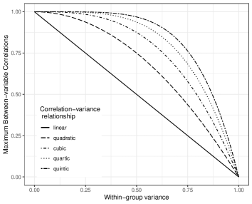
Figure 3: Correlation-variance relationship for vscc selection criteria, based on Figure 1 in Andrews and McNicholas (2014).

The vscc algorithm is computationally efficient and performs well on Gaussian clusters. However, because variables are selected based on the minimization of within-cluster variance, this method would suffer substantially when applied to skewed clusters. Herein, we discuss how this algorithm can be extended to skewed data (Section 3) and we compare the extension to the previously-discussed algorithms (Sections 4 and 5).

3 Methodology

3.1 Algorithm

We must transform the data to near-normality for minimization of within-cluster variance to be used as a variable selection criterion for skewed clustering/classification problems. Thus, we propose an extension to vscc where a Manly mixture is fit to the data. The transformation parameters are then obtained from the fitted model and applied to the data prior to conducting the variable selection laid out in vscc. The skewed clustering extension is detailed below in Algorithm 1, where $g=1,\ldots,G$ indexes clusters, $i=1,\ldots,n$ indexes observations, and $j=1,\ldots,p$ indexes variables.

Algorithm 1 VSCC Manly

1:Perform model-based clustering, fitting either a full Manly mixture or a Manly mixture with transformation parameter selection.

2:Use $\hat{z}_{ig}$ as initial group memberships.

3:Transform data according to the following,

$$\mathbf{Y}_{g}=\bigg{(}\frac{e^{\hat{\lambda}_{1g}\mathbf{x}_{1}}-1}{\hat{\lambda}_{1g}},\ldots,\frac{e^{\hat{\lambda}_{pg}\mathbf{x}_{p}}-1}{\hat{\lambda}_{pg}}\bigg{)}.$$

4:Scale transformed variables.

5:Calculate within-group variance for each variable,

$$\hat{W}_{j}=\frac{1}{n}\sum_{g=1}^{G}\sum_{i=1}^{n}\hat{z}_{ig}(y_{ji}-\hat{\mu}_{jg})^{2}.$$

6:Sort $\hat{W}_{j}$ in ascending order.

7:for $\texttt{i in }1:5$ do

8:     $\hat{W}_{1}$ is automatically selected into $V_{(i)}$

9:     for $\texttt{j in }2:p$ do

10:         if $|\rho_{jr}|<1-\hat{W}^{i}_{j}$ for all r in $V_{(i)}$ then

11:              Variable j is placed in $V_{(i)}$

12:         else

13:              Variable j is not placed in $V_{(i)}$

14:         end if

15:     end for

16:end for

17:Perform Manly mixture model-based clustering on all five variable subsets.

18:Select $V_{(i)}$ such that $n-\sum_{i=1}^{n}\max_{g}\{\hat{z}_{ig}\}$ is minimized.

Algorithm 1 details the skewed extension of vscc for clustering problems. For this method to be applied to classification problems, transformation parameters and true group memberships would need to be supplied in replacement of lines 1 and 2 in Algorithm 1.

We note that studies of traditional skewed methods versus transformation methods have found that no one type of method for handling skewness outperforms the other (Gallaugher et al., 2020); thus, the use of a transformation-based mixture model is an appropriate choice for dealing with skewness. Additionally, we select a transformation-based mixture model for extending the vscc algorithm into the skewed space, over a mixture model that deals with skewness directly, to allow for transformations of clusters into the near-normal space.

3.2 Performance Assessment

Performance can be easily measured for simulated data as we know the clustering variables a priori. For real data, there are no true clustering variables; as a result, measuring performance becomes more difficult. We measure performance in three ways: adjusted Rand index (ARI; Hubert and Arabie, 1985), the number of clusters chosen, and visually with variable plots. As the dimension of the selected set increases, it becomes harder to assess performance using visualizations. Regardless, one can still observe redundancy in the selected set and so variable plots remain helpful even in such circumstances. We are operating in the clustering framework; however, true labels exist for all datasets tested. Therefore, the ARI remains a valuable performance assessment tool. The ARI was proposed as to force the Rand index (Rand, 1971) to have expected value of zero under random assignment (Hubert and Arabie, 1985), which leads to a more interpretable index. The ARI equals one when there is perfect agreement between partitions and is negative when the agreement is worse than would be expected via random assignment.

3.3 Model Fitting

All previously discussed methods will be tested on each dataset. To ensure fair comparison between vsccmanly and skewvarsel, we fit both a MSN mixture and a Manly mixture to the variables selected by skewvarsel. An MSN mixture is fitted to remain consistent with Wallace et al. (2018) and with the skewvarsel algorithm — the BIC used for variable selection comes from a MSN mixture.

4 Real Data Results

The vscc, clustvarsel, vsccmanly, and skewvarsel algorithms are compared on four datasets under a clustering framework. All methods will test $G=1,\ldots,9$ and data is standardized prior to running each method.

4.1 Australian Institute of Sport Data

The Australian Institute of Sport (AIS) dataset can be found in the ManlyMix package (Zhu and Melnykov, 2018b). This dataset contains 11 measurements on 202 individuals. Clustering results are compared to the sex column. From Table 1, we find that the vsccmanly algorithms perform the best in terms of $G$ and ARI. More significantly, the vsccmanly-forwards algorithm reduces the dimensions more than all other methods tested. From Figures 4 and 5, we see that the variables selected by the vsccmanly algorithms clearly separate the sexes. All other methods tested appear to be more susceptible to correlated variables, thus creating redundancy in the selected set. The vsccmanly-forwards and vsccmanly-backwards algorithms resulted in the selection of a different final set of variables. Just as forwards and backwards step-wise regression can result in different results, forwards and backwards transformation parameter selection can result in different transformed spaces. Hence, it is unsurprising to see a difference in the set of selected variables.

Table 1: Variables selection results for the AIS data.

Model	$G$	ARI	Variables
vscc	4	0.52	LBM, Bfat, SSF, Wt, Ht, Hg, BMI, RCC, Fe
clustvarsel	7	0.27	LBM, Bfat, Wt
vsccmanly-forward	2	0.94	LBM, Bfat
vsccmanly-backward	2	0.96	LBM, Bfat, Hg
vsccmanly-full	2	0.96	LBM, Bfat, Hg
skewvarsel + MSN	3	0.26	LBM, Bfat, SSF, Wt
skewvarsel + Manly forward	4	0.59	LBM, Bfat, SSF, Wt
skewvarsel + Manly backward	4	0.57	LBM, Bfat, SSF, Wt

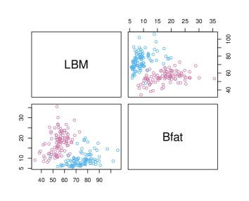
Figure 4: Variables selected by vsccmanly-forwards for the AIS data.

Figure 5: Variables selected by vsccmanly-backwards for the AIS data.

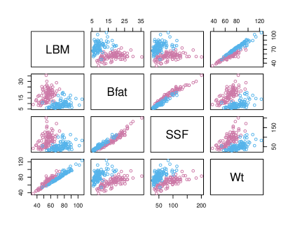
Figure 6: Variables selected by skewvarselfor the AIS data.

4.2 Banknote Data

The banknote dataset comes from the mclust package (Scrucca et al., 2016). There are six measurements, 200 observations, and two types of bills (genuine and counterfeit). Clustering results are compared to bill type. Variable selection on the banknote dataset produces interesting results as no method significantly reduces dimensions (Table 2). This is surprising because, from Figure 7, it appears as though only two variables would be necessary for separating clusters. However, when a Manly mixture is fit to either the variables selected by the skewvarsel or the vscc algorithm, three clusters are found and ARI drops to 0.85. This suggests that although it may seem like the vsccmanly algorithm is selecting too many variables, the algorithm may be selecting the number of variables needed to ensure superior clustering performance.

Table 2: Variable selection results for the banknote data.

Model	$G$	ARI	Variables
vscc	3	0.86	Diagonal, Bottom, Top, Right
clustvarsel	4	0.67	Diagonal, Bottom, Top, Left, Length
vsccmanly-forward	2	0.98	Diagonal, Bottom, Top, Right, Left
vsccmanly-backward	2	0.98	Diagonal, Bottom, Top, Right, Left
vsccmanly-full	2	0.98	Diagonal, Bottom, Top, Right, Left
skewvarsel + MSN	4	0.69	Diagonal, Bottom, Top, Left
skewvarsel + Manly forward	3	0.85	Diagonal, Bottom, Top, Left
skewvarsel + Manly backward	3	0.85	Diagonal, Bottom, Top, Left

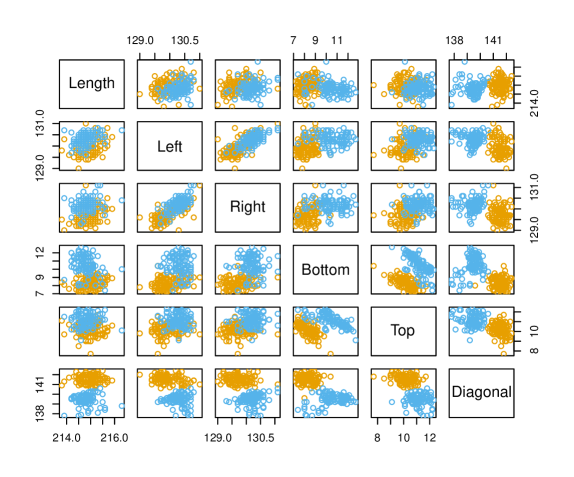
Figure 7: Variables in the banknote data.

4.3 Italian Wine Data

The Italian wine dataset can be found in the pgmm package (McNicholas et al., 2022). It contains 28 variables, 178 observations, and three types of wine to which clustering results are compared. In Table 3, we see that skewvarsel performs the best while vsccmanly performs the worst, in terms of $G$ and ARI. Nearly all methods appear to reduce dimensions approximately the same amount with key variables such as flavanoids and hue being selected nearly every time. This would suggest that it is not the minimization of within-cluster variance that is performing poorly on this dataset but rather the fit of the Manly mixture. This point is further emphasized when we look at the skewvarsel results in Table 3. When the MSN mixture is fit to the skewvarsel selected variables, a much higher ARI is obtained than when the backwards Manly mixture is fit to the same variables. These results suggest that the Manly distribution may be more prone to combining Gaussian clusters to create skewed clusters. As the MSN distribution is normal-like in the tails, the MSN may be less prone to the same behaviour. We see this behaviour in the pairs plots of the Italian wine data selected by vsccmanly-backwards (Figure 9). We replicate this behaviour on simulated data from a three-component, two-dimensional GMM in Figure 10.

Table 3: Variable selection results from the Italian wine dataset.

Model	$G$	ARI	Variables
vscc	3	0.76	Flavanoids, Hue, OD280/OD315 Diluted Wine, Proline, Colour Intensity, Alcohol,Total Phenols, OD280/OD315 of Flavanoids, Uronic Acids, Tartaric Acid, Fixed Acidity, Glycerol, Malic Acid, Alcalinity of Ash, Sugar-free Extract, Proanthocyanins, Phosphate, Non-flavanoid, 2-3-Butanediol, Calcium, Ash, Magnesium, Total Nitrogen, Chloride
clustvarsel	5	0.66	Flavanoids, Proline, Colour Intensity, Uronic Acid, Chloride, Malic Acid
vsccmanly-forward	2	0.43	Flavanoids, Hue, OD280/OD315 Diluted Wine, OD280/OD315 Flavanoids
vsccmanly-backward	2	0.49	Flavanoids, Hue, OD280/OD315 Diluted Wine, Colour Intensity, Uronic Acid
vsccmanly-full	2	0.47	Flavanoids, Hue, OD280/OD315 Diluted Wine, Colour Intensity, Uronic Acid, Total Phenols
skewvarsel + MSN	3	0.80	Flavanoids, Hue, Proline, Colour Intensity, Alcohol, Uronic Acid, Malic Acid, Tartaric Acid
skewvarsel + Manly forward	3	0.73	Flavanoids, Hue, Proline, Colour Intensity, Alcohol, Uronic Acid, Malic Acid,Tartaric Acid
skewvarsel + Manly backward	2	0.46	Flavanoids, Hue, Proline, Colour Intensity, Alcohol, Uronic Acid, Malic Acid, Tartaric Acid

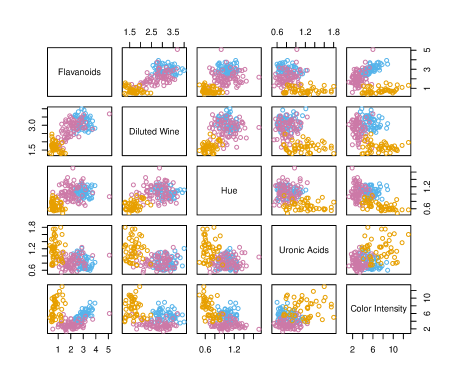
Figure 8: True clustering on variables selected by vsccmanly-backwards for the wine data.

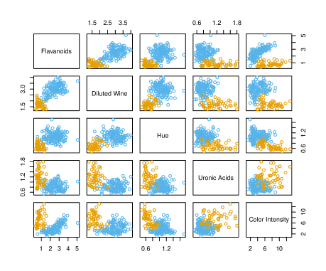
Figure 9: Clustering by vsccmanly-backwards for the wine data.

(a) True clusters (components) simulated data from three-component GMM.

(b) Clustering results for vsccmanly-forwards.

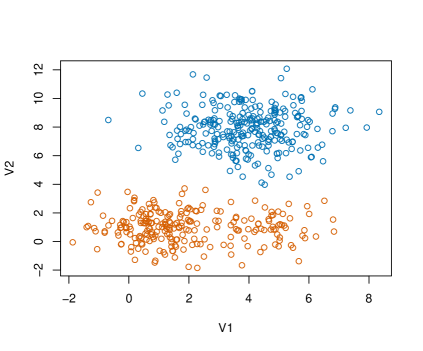
(c) Clustering results for vsccmanly-backwards

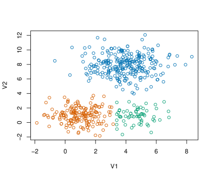
(d) Clustering results for skewvarsel+MSN.

Figure 10: Clustering results from simulated three-component GMM.

4.4 Breast Cancer Wisconsin (Diagnostic)

The breast cancer dataset comes from the UCI Machine Learning Repository (Dua and Graff, 2019). It contains 30 variables, two tumour types (benign and malignant), and 569 observations. Clustering results are compared to tumour type. From Table 4, we see that vsccmanly reduces the dimensions from 30 variables down to one, while selecting the correct number of clusters and obtaining the highest ARI of all methods tested. In particular, we see a large jump in performance, on all three measures, from vscc to its skewed counterpart. We do not see similar improvement in performance by the skewed extension of clustvarsel. Again, we see redundancy in the variables selected by skewvarsel, as seen in Figure 12.

Table 4: Variable selection results for the breast cancer data.

Model	$G$	ARI	Variables
vscc	9	0.16	V7, V8, V9, V10, V11, V12, V13, V14, V17, V18, V19, V20, V21, V22, V26, V28, V29, V30
clustvarsel	4	0.39	V3, V5, V6, V8, V9, V13, V15, V16, V18, V19, V22, V23, V25, V26, V28, V29
vsccmanly-forward	2	0.30	V10, V21
vsccmanly-backward	2	0.63	V30
vsccmanly-full	2	0.50	V16
skewvarsel+ MSN	5	0.33	V3, V6, V13, V16, V23, V26
skewvarsel+ Manly forward	4	0.45	V3, V6, V13, V16, V23, V26
skewvarsel+ Manly backward	3	0.36	V3, V6, V13, V16, V23, V26

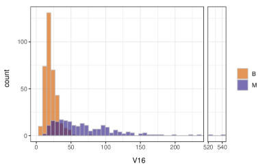
(a) Variables selected by vsccmanly-full.

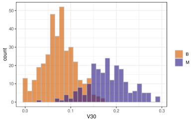
(b) Variables selected by vsccmanly-backwards.

Figure 11: Breast cancer variables selected by vsccmanly.

5 Simulated Data Results

We simulated data from a three-component mixture of multivariate variance-gamma distributions 250 times. An example of this data can be found in Figure 5. To allow us to test for the effect of sample size on method performance, we ran our simulation for $\text{N}\in\{200,500,1000\}$. Using a simulation is helpful as we can artificially create clustering and non-clustering variables to determine how well these methods select important variables and deselect unimportant ones. The simulation specifics are detailed in Table 5, where information on the clustering variables (V1 and V2), nonsense variables (V3 and V4) and the noisy variable (V5) can be found. To reduce the computational time, each model is fit to each simulated dataset only once.

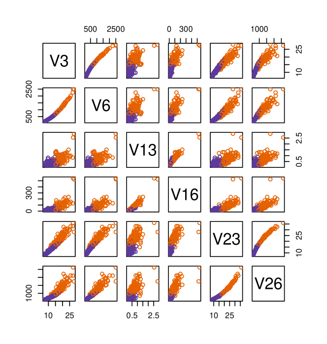
Figure 12: Breast cancer variables selected by skewvarsel.

From Table 5, we see that the vsccmanly-backwards, vsccmanly-full, and skewvarsel algorithms perform the best in terms of average $G$, average ARI, selecting the correct variables (V1 and V2) and removing the nonsense variables (V3 and V4) when $N=500$ and $N=1000$. However, we see a considerable standard deviation of the ARI when $N=200$ for skewvarsel, suggesting a possible instability at smaller sample sizes. The skewvarsel algorithm performs the best on removing the noisy variable (V5) across all sample sizes. Generally, these results agree with the real data results in that the skewed methods greatly improve dimension reduction over their Gaussian counterparts when skewness is present. Unlike the real data results, we see the skewvarsel algorithm performing the best, in terms of dimension reduction, on the simulated data suggesting that this algorithm may suffer in the presence of outliers or deviations from theoretical distributions.

tableInformation on how the simulated data are generated. Variable Type Specifications Clustering $[\mathbf{X}_{1g},\mathbf{X}_{2g}]\sim\text{MVG}(\boldsymbol{\mu}_{g},\boldsymbol{\Sigma}_{g},\boldsymbol{\alpha}_{g},\lambda_{g},\psi_{g})$ $\boldsymbol{\mu}_{1}=\begin{bmatrix}2\\ 3\end{bmatrix}$ $\boldsymbol{\mu}_{2}=\begin{bmatrix}5\\ 3\end{bmatrix}$ $\boldsymbol{\mu}_{3}=\begin{bmatrix}5\\ 15\end{bmatrix}$ $\boldsymbol{\Sigma}_{1}=\begin{bmatrix}1&0\\ 0&1\end{bmatrix}$ $\boldsymbol{\Sigma}_{2}=\begin{bmatrix}1&0\\ 0&1\end{bmatrix}$ $\boldsymbol{\Sigma}_{3}=\begin{bmatrix}2&0\\ 0&2\end{bmatrix}$ $\boldsymbol{\alpha}_{1}=\begin{bmatrix}1\\ 4\end{bmatrix}$ $\boldsymbol{\alpha}_{2}=\begin{bmatrix}4\\ 4\end{bmatrix}$ $\boldsymbol{\alpha}_{3}=\begin{bmatrix}0.1\\ 0.1\end{bmatrix}$ $\lambda_{1}=4$ $\lambda_{2}=4$ $\lambda_{3}=3$ $\chi_{1}=0$ $\chi_{2}=0$ $\chi_{3}=0$ $\psi_{1}=8$ $\psi_{2}=8$ $\psi_{3}=6$ $p_{1}=0.4$ $p_{2}=0.4$ $p_{3}=0.2$ Nonsense $\mathbf{X}_{3}\sim\text{GIG}(3,0,6)$ $\mathbf{X}_{4}\sim\text{GIG}(1,0,2)$ Noisy $\mathbf{X}_{5}=0.6\mathbf{V1}+0.4\mathbf{Z},\ \text{where}\ \mathbf{Z}\sim N(0,5)$

figureExample of simulated data when $N=500$.

Table 5: Summary of simulation results for all approaches.

Method	$N$	$\overline{G}$	$\overline{\text{ARI}}$ (s.d.)	V1	V2	V3	V4	V5
vscc	200	4.6	0.73 (0.14)	250	250	151	193	174
	500	6.4	0.57 (0.1)	250	250	232	249	192
	1000	7.8	0.44 (0.06)	250	250	241	250	175
clustvarsel	200	4.6	0.68 (0.2)	243	244	10	138	0
	500	7.4	0.46 (0.09)	250	250	2	247	0
	1000	8.3	0.41 (0.05)	250	250	18	250	0
vsccmanly-forwards	200	3.02	0.85 (0.2)	234	240	32	18	39
	500	3.7	0.83 (0.14)	250	243	19	41	128
	1000	5	0.68 (0.17)	248	227	8	78	104
vsccmanly-backwards	200	2.9	0.90 (0.14)	239	249	20	18	19
	500	3	0.94 (0.03)	250	250	0	1	107
	1000	3	0.95 (0.01)	250	250	0	0	140
vsccmanly-full	200	2.9	0.90 (0.13)	239	249	25	14	17
	500	3	0.94 (0.03)	250	250	0	1	120
	1000	3	0.95 (0.02)	250	250	0	0	145
skewvarsel+ MSN	200	2.89	0.81 (0.31)	218	218	0	32	3
	500	3.09	0.90 (0.14)	245	245	0	5	0
	1000	3.5	0.87 (0.1)	250	250	0	0	0

6 Discussion

In nearly all instances, we see the skewed extensions of common variable selection algorithms improving performance in the presence of skewness. This improvement in performance is seen not only in the selection of the number of clusters and ARI but, more importantly, in the reduction of dimensions. In the AIS and breast cancer examples, we see more effective dimension reduction by vsccmanly than skewvarsel in terms of the magnitude of dimension reduction and model fitting performance. For the banknote dataset, vsccmanly selects more variables than skewvarsel but also results in a better fitting model, regardless of the model fit to the skewvarsel results. The Italian wine dataset highlights the potential importance of utilizing methods designed for Gaussian clusters when appropriate.

There are instances where vsccmanly may select too many variables to account for some odd observations. For example, we see this in the AIS dataset when the backwards and full Manly mixture extensions select variable Hg. This selection causes some boundary points between groups to switch clusters resulting in one less miss-classification. Although adding this variable improves ARI, the goal of these algorithms is dimension reduction; as such, there may be instances in which smaller ARI is preferred if it corresponds to smaller number of selected variables. One way to account for odd or hard-to-classify observations may be mixtures of contaminated transformation distributions. These component densities contain an inflated secondary component that allows for better modelling of outliers and heavy tails.

One downside to the skewed extensions is computational overhead. The clustvarsel and skewvarsel algorithms are naturally more computationally expensive due to their step-wise nature, with skewvarsel taking longer as more parameters need to be estimated. The vscc algorithm outperforms all methods on computational time as model fitting takes place only on the initial full set and the final sets of variables. This improvement in computational time extends into the skewed space when a full Manly mixture is fit to the data. However, the algorithm slows down greatly under forward or backward transformation parameter selection due to the introduction of some inclusion/exclusion steps. This increase in computational time is heavily influenced by the structure of the clusters and the selection process used. For heavily skewed data, vsccmanly with backwards selection is much faster than its forwards counterpart. If only a few non-zero transformation parameters are necessary, vsccmanly with forwards selection would be much faster. Although more time-consuming than vscc or vsccmanly-full, vsccmanly with transformation parameter selection does tend to perform better than both in terms of ARI and dimension reduction. Thus, we suggest one performs some exploratory analysis on their data before selecting any of these methods to ensure that the algorithm selected is a good fit for their data and the computational overhead is justified. Additionally, the Manly transformation parameter selection is currently programmed in R and could be sped up if programmed in a faster language. Computational time could be further reduced with parallelization of model fitting within each inclusion/exclusion step.

Acknowledgements

This work is supported by a Discovery Grant from the Natural Sciences and Engineering Research Council of Canada, a Dorothy Killam Fellowship, and the Canada Research Chairs program.

References

- Adams and Beling (2019) Adams, S. and P. A. Beling (2019). A survey of feature selection methods for gaussian mixture models and hidden markov models. Artificial Intelligence Review 52(3), 1739–1779.
- Andrews and McNicholas (2014) Andrews, J. L. and P. D. McNicholas (2014). Variable selection for clustering and classification. Journal of Classification 31(2), 136–153.
- Loperfido (2019) Loperfido, N. (2019). Finite mixutres, projection pursuit and tensor rank: a triangulation. Advances in Data Analysis and Classification 13(1), 145–173.
- Redner and Walker (1984) Redner, R. A. and H. F. Walker (1984). Mixture densities, maximum likelihood and the EM algorithm. SIAM Review 26, 195–239.
- Stephens (2000) Stephens, M. (2000). Dealing with label switching in mixture models. Journal of Royal Statistical Society: Series B 62, 795–809.
- Andrews et al. (2023) Andrews, J. L., M. Neal, and P. D. McNicholas (2023). vscc: Variable Selection for Clustering and Classification. R package version 0.5.
- Barndorff-Nielsen et al. (1982) Barndorff-Nielsen, O., J. Kent, and M. Sørensen (1982). Normal variance-mean mixtures and z distributions. International Statistical Review 50(2), 145–159.
- Bouveyron and Brunet-Saumard (2014) Bouveyron, C. and C. Brunet-Saumard (2014). Model-based clustering of high-dimensional data: A review. Computational Statistics and Data Analysis 71, 52–78.
- Box and Cox (1964) Box, G. E. and D. R. Cox (1964). An analysis of transformations. Journal of the Royal Statistical Society: Series B (Methodological) 26(2), 211–243.
- Browne and McNicholas (2015) Browne, R. P. and P. D. McNicholas (2015). A mixture of generalized hyperbolic distributions. Canadian Journal of Statistics 43(2), 176–198.
- Dua and Graff (2019) Dua, D. and C. Graff (2019). UCI machine learning repository.
- Fop and Murphy (2018) Fop, M. and T. B. Murphy (2018). Variable selection methods for model-based clustering. Statistics Surveys 12, 18–65.
- Franczak et al. (2014) Franczak, B. C., R. P. Browne, and P. D. McNicholas (2014). Mixtures of shifted asymmetric Laplace distributions. IEEE Transactions on Pattern Analysis and Machine Intelligence 36(6), 1149–1157.
- Gallaugher et al. (2020) Gallaugher, M. P. B., P. D. McNicholas, V. Melnykov, and X. Zhu (2020). Skewed distributions or transformations? modelling skewness for a cluster analysis.
- Hubert and Arabie (1985) Hubert, L. and P. Arabie (1985). Comparing partitions. Journal of Classification 2(1), 193–218.
- Nelder and Mead (1965) Nelder, J.A.. and R. Mead (1965). A Simplex Method for Function Minimization The Computer Journal 7(1), 308-313.
- Hennig (2023) Hennig, C. (2023). Parameters not empirically identifiable or distinguishable, including correlation between Gaussian observations. Statistical Papers 2(1), 1–24.
- Koot et al. (2013) Koot, M., M. Mandjes, G. van’t Noordende, and C. De Laat (2013). A probabilistic perspective on re-identifiability. Mathematical Population Studies 20(3), 155–171.
- Karlis and Santourian (2009) Karlis, D. and A. Santourian (2009). Model-based clustering with non-elliptically contoured distributions. Statistics and Computing 19(1), 73–83.
- Kass and Raftery (1995) Kass, R. E. and A. E. Raftery (1995). Bayes factors. Journal of the American Statistical Association 90(430), 773–795.
- Lo and Gottardo (2012) Lo, K. and R. Gottardo (2012). Flexible mixture modeling via the multivariate t distribution with the box-cox transformation: an alternative to the skew-t distribution. Statistics and computing 22(1), 33–52.
- Maugis et al. (2009) Maugis, C., G. Celeux, and M.-L. Martin-Magniette (2009). Variable selection for clustering with Gaussian mixture models. Biometrics 65(3), 701–709.
- McNicholas (2016a) McNicholas, P. D. (2016a). Mixture Model-Based Classification. Boca Raton: Chapman & Hall/CRC Press.
- McNicholas (2016b) McNicholas, P. D. (2016b). Model-based clustering. Journal of Classification 33(3), 331–373.
- McNicholas et al. (2022) McNicholas, P. D., A. ElSherbiny, A. F. McDaid, and T. B. Murphy (2022). pgmm: Parsimonious Gaussian Mixture Models. R package version 1.2.6.
- McNicholas et al. (2017) McNicholas, S. M., P. D. McNicholas, and R. P. Browne (2017). A mixture of variance-gamma factor analyzers. In S. E. Ahmed (Ed.), Big and Complex Data Analysis: Methodologies and Applications, pp. 369–385. Cham: Springer International Publishing.
- Pyne et al. (2009) Pyne, S., X. Hu, K. Wang, E. Rossin, T.-I. Lin, L. M. Maier, C. Baecher-Allan, G. J. McLachlan, P. Tamayo, D. A. Hafler, P. L. D. Jager, and J. Mesirow (2009). Automated high-dimensional flow cytometric data analysis. Proceedings of the National Academy of Sciences 106, 8519–8524.
- R Core Team (2023) R Core Team (2023). R: A Language and Environment for Statistical Computing. Vienna, Austria: R Foundation for Statistical Computing.
- Raftery and Dean (2006) Raftery, A. E. and N. Dean (2006). Variable selection for model-based clustering. Journal of the American Statistical Association 101(473), 168–178.
- Rand (1971) Rand, W. M. (1971). Objective criteria for the evaluation of clustering methods. Journal of the American Statistical Association 66(336), 846–850.
- Schwarz (1978) Schwarz, G. (1978). Estimating the dimension of a model. The Annals of Statistics 6(2), 461–464.
- Scrucca et al. (2016) Scrucca, L., M. Fop, T. B. Murphy, and A. E. Raftery (2016). mclust 5: clustering, classification and density estimation using Gaussian finite mixture models. The R Journal 8(1), 289–317.
- Scrucca and Raftery (2018) Scrucca, L. and A. E. Raftery (2018). clustvarsel: A package implementing variable selection for gaussian model-based clustering in r. Journal of Statistical Software 84(1), 1–28.
- Steinley and Brusco (2008) Steinley, D. and M. J. Brusco (2008). Selection of variables in cluster analysis: An empirical comparison of eight procedures. Psychometrika 73, 125–144.
- Steinley and Brusco (2011) Steinley, D. and M. J. Brusco (2011). K-means clustering and mixture model clustering: Reply to mclachlan (2011) and vermunt (2011). Psychological Methods 16(1), 89–92.
- Wallace et al. (2018) Wallace, M. L., D. J. Buysse, A. Germain, M. H. Hall, and S. Iyengar (2018). Variable selection for skewed model-based clustering: application to the identification of novel sleep phenotypes. Journal of the American Statistical Association 113(521), 95–110.
- Zhu and Melnykov (2018a) Zhu, X. and V. Melnykov (2018a). Manly transformation in finite mixture modeling. Computational Statistics & Data Analysis 121, 190–208.
- Zhu and Melnykov (2018b) Zhu, X. and V. Melnykov (2018b). ManlyMix: An R Package for Model-Based Clustering with Manly Mixture Models. R package version 0.1.14.