SketchOGD: Memory-Efficient Continual Learning

Abstract

When machine learning models are trained continually on a sequence of tasks, they are liable to forget what they learned on previous tasks—a phenomenon known as catastrophic forgetting. Proposed solutions to catastrophic forgetting tend to involve storing information about past tasks, meaning that memory usage is a chief consideration in determining their practicality. This paper proposes a memory-efficient solution to catastrophic forgetting, improving upon an established algorithm known as orthogonal gradient descent (OGD). OGD utilizes prior model gradients to find weight updates that preserve performance on prior datapoints. However, since the memory cost of storing prior model gradients grows with the runtime of the algorithm, OGD is ill-suited to continual learning over arbitrarily long time horizons. To address this problem, this paper proposes SketchOGD. SketchOGD employs an online sketching algorithm to compress model gradients as they are encountered into a matrix of a fixed, user-determined size. In contrast to existing memory-efficient variants of OGD, SketchOGD runs online without the need for advance knowledge of the total number of tasks, is simple to implement, and is more amenable to analysis. We provide theoretical guarantees on the approximation error of the relevant sketches under a novel metric suited to the downstream task of OGD. Experimentally, we find that SketchOGD tends to outperform current state-of-the-art variants of OGD given a fixed memory budget.

1 Introduction

Humans learn continually. We gain new capabilities without needing to retrain on familiar tasks. Skills learned in one scenario often transfer to another. Also, we learn relatively robustly even under the presence of distribution shifts that occur naturally during our lifespan [1, 2]. However, imbuing artificial agents based on deep neural networks with this ability to learn continually is complicated by a phenomenon known as catastrophic forgetting [3]: in the naïve approach of training networks on tasks one by one, performance on previous tasks can drop drastically when new tasks are encountered.

One of the most important requirements for a continual learning algorithm intended to overcome catastrophic forgetting is that it be memory-efficient. Various approaches have been proposed to combat catastrophic forgetting (as briefly introduced in Section 1.1). These approaches tend to involve storing information about past tasks to preserve trained knowledge while learning new tasks. Since continual or lifelong learning frameworks should consider learning new tasks over arbitrarily long time horizons with fixed memory budgets, memory cost is a chief consideration for practicality.

To push the frontier in memory-efficient continual learning, this paper focuses on an established continual learning algorithm known as orthogonal gradient descent [4, OGD]. Building on the properties of overparameterized neural networks [5, 6, 7, 8], OGD preserves performance on previous tasks by storing model gradients for previous training examples and projecting later weight updates into the subspace orthogonal to those gradients. We choose to focus on OGD because it is simple, effective, and amenable to analysis. Furthermore, unlike other continual learning algorithms such as A-GEM [9], it does not require re-computing forward passes on old tasks meaning that there is no need to store raw datapoints. This reduces computation requirements and may be beneficial in a setting where privacy is important. However, a key limitation of OGD is the memory cost of storing large numbers of gradients. For a model with $p$ parameters trained for $T$ iterations, the memory requirement is $\mathcal{O}(pT)$. For deep overparameterized networks, $p$ itself may be large, and the growth in the memory requirement with $T$ makes OGD ill-suited to learning over long time horizons.

To resolve the memory issues of OGD, this paper proposes a memory-efficient continual learning algorithm called sketched orthogonal gradient descent—or SketchOGD. More specifically, we leverage sketching algorithms [10] to compress the past model gradients required by OGD into a lower-dimensional representation known as a sketch. Crucially, we can update the sketch efficiently (without needing to decompress and recompress gradients already encountered) such that SketchOGD can run online. In short, SketchOGD avoids storing the full history of past gradients by maintaining a sketch of a fixed size that may be updated cheaply and online. To ensure that SketchOGD is a viable continual learning algorithm, we need to characterize how effective the sketching is in compressing past gradients. We tackle this question both theoretically and experimentally. More specifically, our contributions are as follows:

1. We propose SketchOGD, which addresses the memory inefficiency of OGD by leveraging matrix sketching. In particular, we devise three variants, each employing a different sketching technique.

2. On the theoretical side, we provide formal guarantees on the approximation error of the three proposed variants of SketchOGD. These guarantees depend on the spectral structure of the matrix composed of past gradients and help to inform which sketching variant is best to use.

3. We experimentally benchmark SketchOGD against existing memory-efficient OGD variants and demonstrate that SketchOGD tends to outperform other OGD variants.

1.1 Related Work

Continual learning

Research on lifelong and continual learning focuses on solving the problem of catastrophic forgetting [3, 11]. Some approaches are based on rehearsing old data/experiences whilst learning new tasks [12, 13, 14, 15, 16, 17] or allocating neural resources incrementally for new tasks [18, 19, 20, 21], while others rely on regularizing training to preserve performance on earlier tasks [22]. Orthogonal gradient descent is one such regularization-based approach, which we discuss in Section 2.1. Other methods include elastic weight consolidation (EWC) [22], synaptic intelligence [23] and averaged gradient episodic memory (A-GEM) [9]. Parisi et al. [24] provide a more thorough review of recent developments. A variant of OGD, known as ORFit, was recently proposed by Min et al. [25] for the special setting of one-pass learning.

Matrix approximation

Many approaches have been proposed for approximating or compressing a matrix, including techniques based on sparsification and quantization [26], column selection [27], dimensionality reduction [28] and approximation by submatrices [29]. One practical form of dimensionality reduction known as sketching is introduced in Section 2.2. Halko et al. [28] provide a brief survey of the matrix approximation literature. Sketching has also been successfully employed for summarizing the curvature of neural networks for the purpose of out-of-distribution detection [30], motivating its application to OGD.

2 Background

2.1 Orthogonal Gradient Descent

As a continual learning algorithm, orthogonal gradient descent (OGD) attempts to preserve predictions on prior training examples as new training examples are encountered. To accomplish this, OGD stores the gradient of the model outputs for past training examples and projects future updates into the subspace orthogonal to these stored gradients. This locally prevents new updates from changing what the model outputs on previous tasks.

To be more precise, given a model $f$ with weights $w\,{\in}\,\mathbb{R}^{p}$, OGD stores the gradients $\nabla_{w}f(x_{1},w),...,\nabla_{w}f(x_{n},w)$ for training examples $x_{1},...,x_{n}$. This paper focuses on classification, and only the gradients of the ground-truth logit are stored which has been found to improve performance empirically [4]. The $n$ gradient vectors are arranged into a matrix $G\in\mathbb{R}^{p\times n}$, and future weight updates are projected onto the orthogonal subspace $(\operatorname{range}G)^{\perp}$. To perform the projection, one may form an orthonormal basis for $\operatorname{range}G$. Letting $\operatorname{orth}G$ denote a matrix whose columns form such a basis, then the OGD weight update may be written as

$$w\leftarrow w+(I-\operatorname{orth}G(\operatorname{orth}G)^{\top})\Delta w.$$

A major limitation of OGD is the memory requirement of storing all $n$ past gradients, where the number of trained examples $n$ grows with the runtime of the algorithm. A simple solution is to only store a random subset of past gradients, in the hope that the corresponding submatrix of $G$ will accurately approximate the range of the full $G$ matrix. We call this method RandomOGD.

Another solution called PCA-OGD has been proposed [31], which stores only the top principal components of the gradients for each task. Similarly, ORFit [25] uses incremental PCA to derive a variant of OGD that is specialized for one-pass learning. Incremental PCA could be directly applied to OGD to compress the memory to a fixed size in an online manner. However, its choice of which principal components to discard, and thus, the quality of compression, is sensitive to the order in which the training data is encountered. The next section introduces an alternative means of approximation that avoids this issue.

2.2 Matrix Approximation via Sketching

To reduce the memory cost of OGD, we use sketch, which approximates a matrix in lower dimensions:

Definition 2.1.

A sketch $(\Omega,\Psi,Y,W)$ of a matrix $A\in\mathbb{R}^{m\times n}$ is an approximation formed by first drawing two i.i.d. standard normal matrices $\Omega\in\mathbb{R}^{n\times k}$ and $\Psi\in\mathbb{R}^{l\times m}$ for $k\leq m$ and $l\leq m$ with $k\leq l$, and then forming the products: $Y=A\Omega\in\mathbb{R}^{m\times k},W=\Psi A\in\mathbb{R}^{l\times n}.$

A sketch can form an approximation $\widehat{A}\in\mathbb{R}^{m\times n}$ to the original matrix $A\in\mathbb{R}^{m\times n}$. For example:

Informal Proposition 2.2 (Direct approximation).

Given a sketch $(\Omega,\Psi,Y,W)$ of a matrix $A\in\mathbb{R}^{m\times n}$, and letting $Q=\operatorname{orth}Y\in\mathbb{R}^{m\times k}$, $\widehat{A}\vcentcolon=Q(\Psi Q)^{\dagger}W$ approximates $A$.

Rigorous justification for this is given by Tropp et al. [10]. The quality of the approximation improves with the size of the sketch set by $k$ and $l$. Especially, $k$ determines the rank of $\widehat{A}$.

For the purposes of OGD, we only need to know the range of the gradient matrix. So, we want to extract the range of $A$ from its sketch. While using $\operatorname{range}\widehat{A}$ would seem natural, care must be taken that $\widehat{A}$ does not include spurious directions in its range, i.e., $\operatorname{range}\widehat{A}\not\supset\operatorname{range}A$. In fact, we have:

$$\operatorname{range}\widehat{A}\subseteq\operatorname{range}Q=\operatorname{range}Y\subseteq\operatorname{range}A.$$

So, $\operatorname{range}Q$ alone approximates $\operatorname{range}A$. When $A$ is symmetric, we can use another approximation:

Informal Proposition 2.3 (Symmetric approximation).

Given a sketch $(\Omega,\Psi,Y,W)$ of a symmetric matrix $A\in\mathbb{R}^{m\times m}$, let $Q=\operatorname{orth}Y\in\mathbb{R}^{m\times k}$ and define $X\vcentcolon=(\Psi Q)^{\dagger}W\in\mathbb{R}^{k\times m}$. Then, $\widehat{A}_{\mathrm{sym}}\vcentcolon=\tfrac{1}{2}(QX+X^{\top}Q^{\top})$ approximates $A$.

Formal justification is again given by Tropp et al. [10]. To approximate $\operatorname{range}A$, we can use the range of the concatenation $[Q\;X^{\top}]$ from this proposition as we observe that:

$$\operatorname{range}\widehat{A}_{\mathrm{sym}}\subseteq\operatorname{range}Q\cup\operatorname{range}X^{\top}\subseteq\operatorname{range}Y\cup\operatorname{range}W^{\top}\subseteq\operatorname{range}A\cup\operatorname{range}A^{\top}=\operatorname{range}A,$$

where the last statement follows since $A$ is symmetric.

3 Sketched Orthogonal Gradient Descent

This section applies the matrix sketching methods introduced in Section 2.2 to obtain three variants of sketched orthogonal gradient descent (SketchOGD). We propose different variants as it is a priori unclear which performs best, but we will investigate this both by presenting theoretical bounds (Section 4.2) and by running experiments (Section 5). All variants adopt the following pattern:

1. Before training on a new task, use the maintained sketch to extract an orthonormal basis that approximately spans $\operatorname{range}G$, where $G$ is the matrix of gradients from previous tasks.

2. While training on the new task, project weight updates to be orthogonal to the orthonormal basis.

3. After the training, calculate gradients of the model’s correct logit and update the sketch.

Algorithm 1 SketchOGD. The algorithm requires a model with weight vector $w$, a base optimizer such as SGD, as well as sketching subroutines from Sketching Method 1, 2 or 3.

  $\mathtt{InitializeSketch}()$

  for task in $\mathbf{\{1,2,...,T\}}$ do

     if task $\geq 2$ then

        $B\leftarrow\mathtt{ExtractBasisFromSketch}()$

     else

        $B\leftarrow 0$

     for each training iteration do

        $\Delta w\leftarrow\mathtt{BaseOptimizerUpdate}()$

        $w\leftarrow w+(I-BB^{\top})\Delta w$

     for each of $\mathbf{s}$ random training points do

        $\triangleright$ Let $g$ denote the gradient of the correct logit

        $\mathtt{UpdateSketch}(g)$

Sketching Method 1 Sketch of gradient matrix $G$.

  def $\mathtt{InitializeSketch}()$:

  Set $Y\in\mathbb{R}^{p\times k}$ to zero

  def $\mathtt{UpdateSketch}(g)$:

  Draw $\omega\in\mathbb{R}^{k}$ i.i.d. standard normal

  $Y\leftarrow Y+g\omega^{\top}$

  def $\mathtt{ExtractBasisFromSketch}()$:

  return  $\operatorname{orth}Y$

Sketching Method 2 Sketch of product $GG^{\top}$.

  def $\mathtt{InitializeSketch}()$:

  Set $Y\in\mathbb{R}^{p\times k}$ to zero

  Draw $\Omega\in\mathbb{R}^{p\times k}$ i.i.d. standard normal

  def $\mathtt{UpdateSketch}(g)$:

  $Y\leftarrow Y+g(g^{\top}\Omega)$

  def $\mathtt{ExtractBasisFromSketch}()$:

  return  $\operatorname{orth}Y$

Sketching Method 3 Symmetric sketch of product $GG^{\top}$.

  def $\mathtt{InitializeSketch}()$:

  Set $Y\in\mathbb{R}^{p\times k}$ and $W\in\mathbb{R}^{l\times p}$ to zero

  Draw $\Omega\in\mathbb{R}^{p\times k}$ and $\Psi\in\mathbb{R}^{l\times p}$ i.i.d. standard normal

  def $\mathtt{UpdateSketch}(g)$:

  $Y\leftarrow Y+g(g^{\top}\Omega)$

  $W\leftarrow W+(\Psi g)g^{\top}$

  def $\mathtt{ExtractBasisFromSketch}()$:

  $Q\leftarrow\operatorname{orth}Y$

  $U,T\leftarrow\mathtt{QR}(\Psi Q)$

  $X\leftarrow T^{\dagger}(U^{\top}W)$

  return  $\operatorname{orth}[Q\;X^{\top}]$

This procedure is described formally in Algorithm 1. Three variants are obtained by using either Sketching Method 1, 2 or 3 to supply the subroutines $\mathtt{InitializeSketch}$, $\mathtt{UpdateSketch}$ and $\mathtt{ExtractBasisFromSketch}$. The variants arise since there is freedom in both which matrix is sketched and what sketching technique is used. For instance, since $G$ and $GG^{\top}$ have the same range, either matrix may be sketched to approximate $\operatorname{range}G$. Furthermore, since $GG^{\top}$ is symmetric, Proposition 2.3 may be applied. To elaborate, we propose three variants of SketchOGD:

SketchOGD-1: Algorithm 1 + Sketching Method 1. This algorithm directly sketches the gradient matrix $G$ via Proposition 2.2, and $\operatorname{orth}Y$ for $Y=G\Omega$ forms the orthonormal basis. When a new gradient $g$ is received, we update $Y$ online instead of recomputing it from scratch since $Y^{(new)}=G^{(new)}\Omega^{(new)}=[G\;g]\begin{bmatrix}\Omega\\ \omega^{\top}\end{bmatrix}=Y+g\omega^{\top}$. Here, the random matrix $\Omega$ is incremented with a standard normal vector $\omega$ since the dimension of $G$ is changed. In terms of memory, SketchOGD-1 needs to store only $Y$ at a cost of $pk$.

SketchOGD-2: Algorithm 1 + Sketching Method 2. This algorithm sketches the product $GG^{\top}$ via Proposition 2.2 as in SketchOGD-1. To update the sketch variable $Y=GG^{\top}\Omega$ online when a new gradient $g$ is received, we leverage the decomposition $Y^{(new)}=G^{(new)}{G^{(new)}}^{\top}\Omega=\sum_{c\in G}cc^{\top}\Omega=Y+gg^{\top}\Omega$ where the summation is running over the columns of $G$. In terms of memory, SketchOGD-2 needs to store both $Y$ and $\Omega$ at a cost of $2pk$.

SketchOGD-3: Algorithm 1 + Sketching Method 3. This algorithm sketches the product $GG^{\top}$ via symmetric sketch (Proposition 2.3). The sketch variables $Y$ and $W$ are updated online using the decomposition of $GG^{\top}$ as in SketchOGD-2. The computation of the pseudoinverse $(\Psi Q)^{\dagger}$ is expedited by first taking the orthogonal-triangular ($\mathtt{QR}$) decomposition. The full sketch needs to be stored, at a memory cost of $2p(l+k)$. Since $l\geq k$, this is at least four times that of SketchOGD-1. However, the basis returned by Sketching Method 3 spans a higher-dimensional subspace.

Overall, SketchOGD-1 is at least twice as memory efficient as the other two methods, so we expect by default for it to do well under the same memory constraint. However, SketchOGD-2,3 may have a higher quality sketch by leveraging the symmetric structure of $GG^{\top}$.

4 Bounds on Sketching Accuracy

This section theoretically analyzes the suitability of the sketching methods for use in SketchOGD.

4.1 Constructing a Metric Suited to SketchOGD

To assess the effectiveness of a sketching method, an error metric is needed. In continual learning, the goal is to preserve performance on all data points previously encountered. Therefore, in the context of SketchOGD, it makes sense to measure sketching accuracy as a sum of errors incurred on each past data point. We propose the following metric:

Definition 4.1 (Error in a sketching method).

Given a matrix $G$ to be approximated and a matrix $B$ returned by a sketching method, the reconstruction error is given by:

$$\mathcal{E}_{G}(B)=\sum_{g\in G}\|g-\operatorname{proj}_{B}g\|_{2}^{2}=\|(1-\operatorname{proj}_{B})G\|_{F}^{2},$$

where the summation is running over the columns of G. In SketchOGD, if the metric vanishes while $\operatorname{range}B\subseteq\operatorname{range}G$, then SketchOGD is equivalent to OGD.

Let us distinguish Definition 4.1 from other possible error metrics. A common way to assess error in the sketching literature is to use a sketch to compute an approximation $\widehat{A}$ to a matrix $A$, and then to report the Frobenius reconstruction error $\|\widehat{A}-A\|_{F}$. The advantage of Definition 4.1 over this is that it decouples the matrix that is sketched from the matrix $G$ that we would like to reconstruct. In particular, the matrix $B$ may be obtained from a sketch of $GG^{\top}$ rather than $G$ itself.

Another possible metric is the Grassmann distance between subspaces [32], which could be applied to measure the distance between the subspace $\operatorname{range}G$ and the subspace $\operatorname{range}B$, where $B$ is returned by the sketching method. The drawback to this approach is that it neglects how the columns $\{g\in G\}$ are distributed within $\operatorname{range}G$. If certain directions appear more frequently, then it is more important for OGD that these directions are well-modeled.

4.2 Deriving Bounds

We now provide a novel theoretical analysis of sketching applied to continual learning, through bounding our metric. While Tropp et al. [10] analyzed the Frobenius reconstruction error of sketching $\mathbb{E}\|A-\widehat{A}\|_{F}^{2}$, and Doan et al. [31] bounded catastrophic forgetting, to our knowledge we are the first to theoretically analyze the disruption a compression method causes to OGD, specifically.

Bounding our metric will depend on the sketching method involved. For the basic, first sketching method, we can adapt a result of Halko. However, for the second and third methods, which sketch $GG^{\top}$ instead of $G$, we state and prove original bounds. In all three cases, our bounds will use some shared notation, including decomposing $G$ and splitting matrices along an index $\gamma$.

Definition 4.2 (Split SVD).

Define $U\in\mathbb{R}^{p\times p},\Sigma_{G}\in\mathbb{R}^{p\times n},V\in\mathbb{R}^{n\times p}$ as the singular value decomposition (SVD) of $G$ such that $G=U\Sigma_{G}V$, where $n$ is the number of sketched gradients. Then, we can define $\Sigma\vcentcolon=\Sigma_{G}\Sigma_{G}^{\top}\in\mathbb{R}^{p\times p}$ such that $GG^{\top}=U\Sigma U^{\top}$. Assuming singular values sorted in decreasing magnitude, we define $\Sigma_{1},\Sigma_{2},U_{1},U_{2}$ by splitting matrices at an index $\gamma\leq k-2$:

$$\Sigma=\begin{bmatrix}\Sigma_{1}&0\\ 0&\Sigma_{2}\end{bmatrix},\qquad U=\begin{bmatrix}U_{1}&U_{2}\end{bmatrix}.$$

Theoretical bounds on our metric based on this split would imply their dependence on the singular value decay of the gradients. In the basic sketching method where we directly sketch the matrix of gradients $G$, we can adapt a theorem of [28] as below. See the appendix for the proof.

Theorem 4.1 (Expected error in Sketching Method 1).

Given that we create a sketch $\widehat{G}$ of $G$ with rank $k$ in accordance with Sketching Method 1, and use the setup described in Definition 4.2, then the expected value of the metric $\mathcal{E}_{G}(\widehat{G})$ has an upper bound: $\mathbb{E}[\mathcal{E}_{G}(\widehat{G})]\leq\min_{\gamma\leq k-2}(1+\tfrac{\gamma}{k-\gamma-1})\cdot\operatorname{Tr}{\Sigma_{2}}.$

Remark 4.3.

Note that sharper decays push the optimal split location $\gamma$ away from $0$. For intuition, consider a flat spectral decay such that $\Sigma=\lambda I_{p\times p}$ for some $\lambda>0$ and the identity matrix $I_{p\times p}$. Then, $\gamma=0$ attains the minimum of the upper bound $p\lambda$. On the other hand, if $\Sigma=\Sigma_{G}\Sigma_{G}^{T}$ has linearly decaying spectral decay from $2\lambda$ to $0$, then $\gamma=2(k{-}1){-}p$ attains the minimum approximately at $\frac{4\lambda}{p}(k{-}1)(p{-}k{+}1)$ for large enough $k$. Analysis can be found in the appendix.

We now provide two novel theorems for Sketching Method 2, one upper bounding the metric deterministically and the other in expectation. See the appendix for the proofs.

Theorem 4.2 (Deterministic error in Sketching Method 2).

We define $G,\Sigma_{1},\Sigma_{2},U_{1},U_{2}$ as in Definition 4.2 for a sketch parameter $k$ and split position $\gamma\leq k-2$. If we create a sketch $(\Omega,\Psi,Y,W)$ and reconstruction $\widehat{A}$ of $A=GG^{\top}$ in accordance with Sketching Method 2, we can use $\Omega\in\mathbb{R}^{p\times k}$ to define: $\Omega_{1}:=U_{1}^{\top}\Omega$, $\Omega_{2}:=U_{2}^{\top}\Omega$. Assume $\Omega_{1}\in\mathbb{R}^{\gamma\times k}$ is full-rank. Then, if $\gamma$ is greater than the rank of $G$, then the metric $\mathcal{E}_{G}(\widehat{A})=0$. Else, $\mathcal{E}_{G}(\widehat{A})\leq\|\Sigma_{2}\Omega_{2}\Omega_{1}^{\dagger}\Sigma_{1}^{-1/2}\|_{F}^{2}+\|\Sigma_{2}^{1/2}\|_{F}^{2}$.

By evaluating the expected value of the bound in Theorem 4.2, we get the following result.

Theorem 4.3 (Exptected error in Sketching Method 2).

We define $G,\Sigma_{1},\Sigma_{2},U_{1}$ as in Definition 4.2 for a sketch parameter $k$ and arbitrary split position $\gamma\leq k-2$. We create a sketch $(\Omega,\Psi,Y,W)$ and reconstruction $\widehat{A}$ of $A=GG^{\top}$, and define $\Omega_{1}:=U_{1}^{\top}\Omega$ as in Theorem 4.2. We assume $\Omega_{1}$ has full rank. Then, if $\gamma$ is greater than the rank of $G$, then the metric $\mathbb{E}[\mathcal{E}_{G}(\widehat{A})]=0$. Else,

$$\mathbb{E}[\mathcal{E}_{G}(\widehat{A})]\leq\min_{\gamma\leq k-2}\tfrac{\gamma}{k-\gamma-1}\operatorname{Tr}(\Sigma_{2}^{2})\operatorname{Tr}(\Sigma_{1}^{-1})+\operatorname{Tr}(\Sigma_{2}).$$

Remark 4.4.

Note that this is a tighter bound than Theorem 4.1 when $\operatorname{Tr}(\Sigma_{2}^{2})\operatorname{Tr}(\Sigma_{1}^{-1})\leq\operatorname{Tr}(\Sigma_{2})$.The smaller the lower singular values are, and the larger the higher singular values are, the more advantageous this bound becomes. One illustrative example is a step-decaying spectral decay such that $\Sigma_{1}=100I_{10\times 10}$ and $\Sigma_{2}=2I_{100\times 100}$. Then, $\operatorname{Tr}(\Sigma_{2}^{2})\operatorname{Tr}(\Sigma_{1}^{-1})=40\leq 200=\operatorname{Tr}(\Sigma_{2})$.

Sketching Method 3 is a modification of Sketching Method 2 to take advantage of the symmetric structure of $GG^{\top}$. It turns out that the metric for Sketching Method 3 is always better than for Sketching Method 2 as below, so we can transfer our previous results. See the appendix for the proof.

Theorem 4.4 (Error in Sketching Method 3).

When sketching $A=GG^{\top}$ into $\widehat{A}$ and $\widehat{A}_{\mathrm{\mathrm{sym}}}$ according to Sketching Methods 2 and 3, the metrics obey: $\mathcal{E}_{G}(\widehat{A}_{\mathrm{sym}})\leq\mathcal{E}_{G}(\widehat{A})$.

Consequently, the bounds described in Theorems 4.2 and 4.3 are also upper bounds for the error metric $\mathcal{E}_{G}(\widehat{A}_{\mathrm{sym}})$ and its expected value $\mathbb{E}[\mathcal{E}_{G}(\widehat{A}_{\mathrm{sym}})]$, respectively.

Remark 4.5.

Overall, these bounds suggest that the performance of different sketching methods may vary with the task-dependent structure of spectral decay.

5 Experiments

In this section, we demonstrate the practical performance of SketchOGD on four continual learning benchmarks: Rotated MNIST, Permuted MNIST, and Split MNIST, and Split CIFAR.

Setup

The benchmarks are created using $1,000$ datapoints for each of the $10$ classes of MNIST, and $600$ datapoints for each of the $20$ classes of CIFAR-100. Rotated MNIST consists of $10$ tasks, created by copying and rotating the dataset by multiples of $5$ degrees. Similarly, Permuted MNIST forms $10$ tasks by creating fixed but random permutations of pixels for each task. Split MNIST forms $5$ tasks by splitting the dataset into pairs of digits and treating each pair as a binary $0,1$ classification task. Similarly, Split CIFAR has $20$ tasks of $5$ classes each. Each task is trained for $30$ epochs.

For the setup of our proposed SketchOGD methods, the memory constraints allow $k=1200$ for Method 1, $k=600$ for Method 2, and $k=299,l=301$ for Method 3. We set $k\approx l$ which is empirically found to be more memory-efficient. Effectively, SketchOGD-1 form a rank-$1200$ approximation, while SketchOGD-2 and SketchOGD-3 form around rank-$600$ approximations.

Network Architecture

For MNIST experiments, we use a three-layer fully connected neural network that has $100$ hidden units in the first two layers with ReLU activations and $10$ output logits, totaling $p=113,610$ parameters. For Split CIFAR, we use a LeNet with a hidden-layer size of $500$ for a total of $1,601,500$ parameters. Unlike previous works [4, 31] that create unique heads for each task in Split MNIST, we keep the model fixed to make Split MNIST a harder problem. However, we keep the multi-head architecture for Split CIFAR.

Baselines

We compare the SketchOGD methods with other continual learning methods under the same memory constraint. They include naive SGD for context, a variant of OGD which we call “RandomOGD” that randomly samples gradients to obey the memory constraint, PCA-OGD proposed by [31] that compresses each task’s gradients using PCA, and OGD without memory constraint. We expect naive SGD to perform drastically worse than all other methods because of catastrophic forgetting. RandomOGD should serve as a lower bound, as random sampling is the simplest form of compression. Unconstrained OGD serves as the theoretical maximum if compression methods were lossless, and PCA-OGD is the current state-of-the-art memory-efficient OGD variant.

It is important to note that PCA-OGD is not an online algorithm within a task. It requires temporarily storing all the gradients for a task at once into a big matrix. Then, it performs singular value decomposition and stores the top left singular vectors as a compression. If a task is large enough, storing all the gradients could easily break the memory constraint. Therefore we run two different scenarios; first, a practical one where PCA-OGD accounts for this fault so that it cannot summarize the full dataset while SketchOGD can, taking advantage of its online nature; then, a toy scenario where PCA-OGD and SketchOGD are set to compress the same number of gradients regardless of the memory issue of PCA-OGD to compare their compression quality from the same ingredients.

5.1 Experiment 1: All Methods under the Same Memory Constraint

Table 1: Test accuracy after training on four different continual learning benchmarks, under a fixed memory constraint. A-GEM is shown separately, representing a commonly used algorithm that allows storing previous datapoints across tasks. The mean and standard deviation over 5 runs for each algorithm-benchmark pair are indicated, and exceptional results are bolded. The SketchOGD methods generally outperform the other variants of OGD, while being comparable to each other.

Algorithm	Rotated	Permuted	Split MNIST	Split CIFAR
SketchOGD-1	$0.865\pm 0.004$	$\textbf{0.832}\pm 0.004$	${0.679}\pm 0.004$	${0.676}\pm 0.002$
SketchOGD-2	$\textbf{0.876}\pm 0.004$	$0.826\pm 0.004$	$0.675\pm 0.007$	$0.672\pm 0.002$
SketchOGD-3	$\textbf{0.875}\pm 0.006$	$0.825\pm 0.002$	${0.676}\pm 0.006$	$0.673\pm 0.002$
PCA-OGD	$0.849\pm 0.004$	$0.821\pm 0.004$	$0.673\pm 0.001$	${0.674}\pm 0.002$
RandomOGD	$0.847\pm 0.007$	$0.819\pm 0.002$	$0.667\pm 0.004$	$0.672\pm 0.002$
SGD	$0.792\pm 0.009$	$0.734\pm 0.019$	$0.604\pm 0.003$	$0.649\pm 0.002$
A-GEM	$0.902\pm 0.002$	$0.887\pm 0.001$	$0.905\pm 0.001$	$0.379\pm 0.024$

Figure 1: Accuracy of various continual learning methods on tasks 1, 5, and 9 of the Rotated MNIST benchmark. Each plot shows the initial learning of a task and the subsequent slow forgetting as the model trains on new tasks. As shown, SketchOGD-2,3 perform the best in this scenario.

Figure 2: Plotted singular values of $4800$ gradient vectors extracted from training OGD on the Rotated MNIST benchmark. The x-axis is placed on a log scale for easier viewing, as the decay is too fast to make sense of otherwise. The stable rank of the matrix is shown as a dotted black line, which can be viewed as an effective rank. As shown, even taking a small number of the top singular vectors ($\approx 300$) would encode the majority of the information.

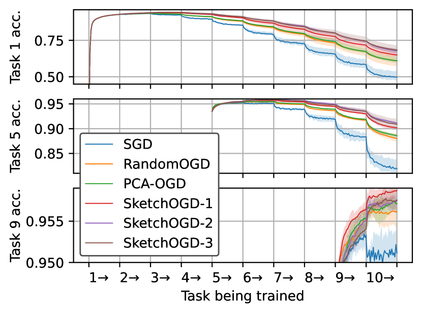
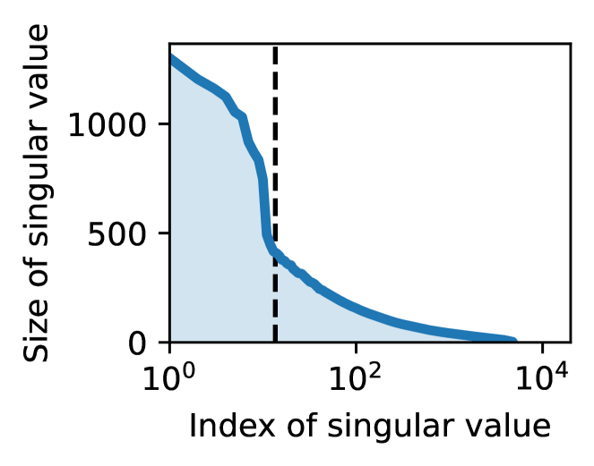
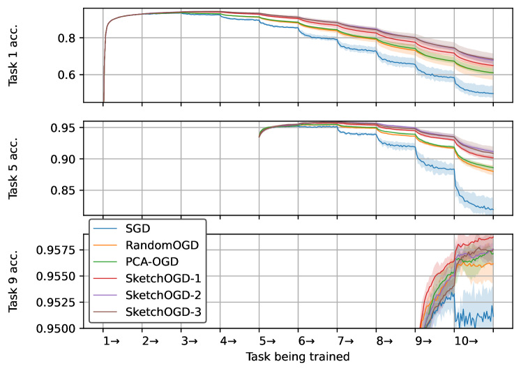
Table 1 shows the first scenario’s results. As sketching more gradients does not change memory costs in SketchOGD, we allow SketchOGD to sketch the full dataset, namely $100,000,10,000$ and $60,000$ gradients, respectively, for Rotated/Permuted MNIST, Split-MNIST, and Split-CIFAR, down to $1200$ vectors. Meanwhile, as PCA-OGD takes extra memory space to run, it can only compress $2000,1500$, and $4000$ gradients down to $1000,900$ and $1000$ vectors, respectively, for the corresponding benchmarks under the same memory constraint. This experiment shows that the SketchOGD methods are comparable to each other, while outperforming PCA-OGD significantly. In addition, the popular continual learning algorithm A-GEM is included for reference, performing well for MNIST benchmarks but extremely poorly for Split CIFAR. Unlike the variants of OGD, A-GEM directly stores datapoints across tasks, which might raise privacy concerns. Figure 2 graphs the test accuracy of tasks $1,5,9$ of the Rotated MNIST benchmark along the training. RandomOGD acts as a simple lower bound for the OGD variants, and the SketchOGD methods outperform PCA-OGD.

5.2 Experiment 2: Compressing the Same Number of Gradients

Table 2: Performance comparison in a toy scenario where each method compresses the same number of gradients; this artificially restricts the capability of SketchOGD to compress arbitrarily many gradients without memory overhead while relatively boosting PCA-OGD. Unlike other methods, OGD is allowed to store all gradients without compression to form an upper bound of lossless compression. The mean and standard deviation of test accuracy over 5 runs for each algorithm-benchmark pair are indicated, and exceptional results are bolded. The SketchOGD methods show comparable performance to PCA-OGD despite the restriction.

Algorithm	Rotated	Permuted	Split MNIST	Split CIFAR
SketchOGD-1	${0.863}\pm 0.005$	$\textbf{0.830}\pm 0.002$	$\textbf{0.684}\pm 0.007$	${0.674}\pm 0.003$
SketchOGD-2	${0.860}\pm 0.006$	$0.818\pm 0.005$	$0.673\pm 0.006$	${0.675}\pm 0.002$
SketchOGD-3	${0.862}\pm 0.007$	$0.812\pm 0.003$	$0.677\pm 0.003$	${0.675}\pm 0.001$
PCA-OGD	${0.864}\pm 0.004$	$\textbf{0.830}\pm 0.002$	$0.678\pm 0.006$	${0.675}\pm 0.002$
RandomOGD	$0.847\pm 0.007$	$0.819\pm 0.002$	$0.667\pm 0.004$	$0.672\pm 0.002$
OGD	$0.888\pm 0.006$	$0.838\pm 0.004$	$0.714\pm 0.002$	$0.675\pm 0.006$

Next, we restrict SketchOGD methods to only being fed in the same number of gradients to compress as PCA-OGD. This is a severe disadvantage as PCA-OGD has a memory overhead to store a full matrix of gradients pre-compression that SketchOGD does not need. Table 2 shows the results where each method compresses $4800$ gradients down to $1200$ vectors, except for OGD, which stores all gradients without compression. In this experiment, we aim to understand how well sketching can compress data in comparison to PCA, as well as the effects of sketching different amounts of gradients on SketchOGD’s results. The sketching methods on balance outperformed RandomOGD and naive SGD, while underperforming the upper bound OGD. Compared to the results in Table 1, while SketchOGD-2,3 drop in performance, SketchOGD-1 is not significantly affected by the reduced number of sketched gradients. Further, even SketchOGD-2,3 are still comparable to PCA-OGD on most benchmarks.

6 Discussion

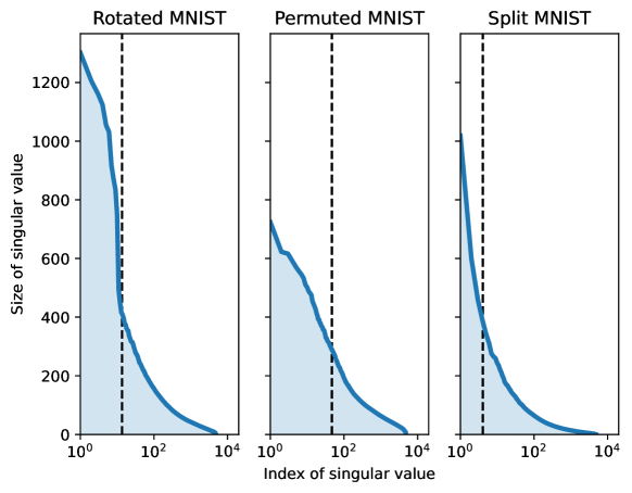
In this section, we discuss the practical performance of the three SketchOGD methods that we propose to accomplish memory-efficient continual learning. Comparing them, no one clearly dominated the other two, while all of them tend to outperform PCA-OGD as seen in Table 1. The similar behavior of SketchOGD-2 and SketchOGD-3 suggests that the doubled memory cost of SketchOGD-3 is counterbalanced by the exploited symmetric structure. Meanwhile, even though SketchOGD-2 has twice the memory cost of SketchOGD-1, it shows better performance in Rotated MNIST. This discrepancy could be explained by the theoretical error bounds derived in Section 4.2 of which relative tightness depends on the spectral decay of the gradients. To elaborate, Figure 2 plots the singular values of the gradients of the Rotated MNIST benchmark. The large first chunk of singular values and sharp decay afterwards benefit the theoretical bounds of SketchOGD-2,3 as noted in Remark 4.4. In contrast, Permuted MNIST has a slower decay (shown in Figure 3 in the appendix), which relatively advantages SketchOGD-1. One may expect the slower decay a priori as the random permutations would interrupt transferring learned features to the following tasks more than other benchmarks, resulting in less similar gradients between tasks. In this manner, intuition about tasks can be utilized in advance to decide which SketchOGD method to use.

Another intuition for the behavior of SketchOGD-2,3 is that the structure of $GG^{\top}$ reflects the gradients with their magnitudes quadratically scaled compared to simply $G$. Then, as larger gradients have more effect on the metric, sketching $GG^{\top}$ may encourage the algorithm to place more importance on larger gradients. This property is particularly effective if there are few key directions (equivalently, a sharper singular value decay). In addition, Table 2 shows that SketchOGD-2,3 benefit more from sketching more gradients, while SketchOGD-1 improves less. This trend could be explained by the theoretical bounds, as Theorem 4.3 is quadratic in the smallest singular values while Theorem 4.1 is linear and therefore is hurt more by additional small singular values.

Lastly, we highlight some important practical concerns that make SketchOGD advantageous over PCA-OGD. First, SketchOGD has a fixed memory usage regardless of how many tasks or gradients we choose to sketch. On the other hand, PCA-OGD increases its memory use for every new task. This makes it hard to predict memory costs and choose the right hyperparameters for PCA-OGD without knowing the number of tasks in advance. In addition, PCA-OGD suffers from the memory overhead to store all gradients for a task before applying PCA. This restricts the comprehensive view of the dataset when the task dataset is large. Secondly, SketchOGD capitalizes on synergies between tasks. As incrementally updating a sketch is equivalent to sketching the full matrix at the start, SketchOGD is effectively summarizing the full gradient matrix containing every single task. Meanwhile, PCA-OGD performs truncated compression on tasks separately. It is likely that different tasks share some directions in their gradients, especially if subsequent tasks have some similarity or connection. Then, sketching the tasks together allows for those shared directions to accumulate in importance and be picked up by the sketch, while a truncated PCA analysis on individual tasks might discard that direction without knowledge of its shared importance with other tasks.

Future Work

Our results motivate several directions of future inquiry. First, Theorem 4.4 leaves room for a more rigorous analysis of the benefits of leveraging the symmetric structure of $GG^{\top}$ in SketchOGD-3. Also, the difference between the bounds in 4.1 and 4.3 involve replacing one instance of $\operatorname{Tr}(\Sigma_{2})$ with $\operatorname{Tr}(\Sigma_{2}^{2})\operatorname{Tr}(\Sigma_{1}^{-1})$; we would like to investigate the way different types of singular value decay would affect these two bounds differently. Another area of importance is one of our potential explanations for SketchOGD-2,3’s performance, namely the quadratically scaled magnitudes of gradients in $GG^{\top}$. We may test whether scaling the gradients by powers of their magnitudes before compression may influence results for the better.

In addition, as one of the key advantages of SketchOGD over PCA-OGD is SketchOGD’s incremental nature, a natural extension of our work is to create a variant of PCA-OGD that uses a more incremental form of PCA, and to test it against SketchOGD. However, any incremental forms of PCA still won’t have the linear properties of sketching that make it equivalent to sketching the full matrix all at once; an incremental modification to PCA will likely still involve repeated truncation, perhaps discarding important directions before they have time to accumulate across tasks.

7 Conclusion

To consider continual learning over long time horizons, memory usage is a practically imperative concern. We proposed SketchOGD, an efficient algorithm for systematically resolving the growing memory problem of orthogonal gradient descent (OGD) in continual learning. Our sketching approach is easy to implement; it maintains a summary of the history of the relevant gradients, which is updated online, without the need to reconstruct a large matrix that may not fit in memory, and without relying on boundaries between the tasks. It uses a constant memory space independent of how many gradients it sketches and therefore can be safely used in scenarios where the future is uncertain. Defining a novel metric for the performance of the sketch, relevant to the downstream task of OGD, we provided formal guarantees on the performance of the sketch by deriving deterministic and in-expectation bounds. Lastly, we showed that SketchOGD outperforms the existing memory-efficient variants of OGD, making it a promising practical algorithm for continual learning with fixed memory.

Appendix A Appendix

A.1 Spectral Decay

Figure 3: Plotted singular values of $4800$ gradient vectors extracted from training OGD on the Rotated MNIST, Permuted MNIST, and Split MNIST classification benchmarks. The x-axis is on a log scale for easier viewing, as the decay is too fast to make sense of otherwise. The stable rank of the matrix is shown as a dotted black line, which can be viewed as an effective rank. Permuted MNIST shows relatively slow spectral decay compared to the other two benchmarks. However, the decay is still sharp enough so that even taking a small number of the top singular vectors ($\approx 300$) would encode the majority of the information for all three benchmarks.

A.1.1 Effects of Spectral Decay on Bounds

Recall that the theoretical upper bound on the expected error metric for SketchOGD-1 is $\min_{\gamma\leq k-2}(1+\tfrac{\gamma}{k-\gamma-1})\cdot\operatorname{Tr}{\Sigma_{2}}$ where $\Sigma_{2}$ is the lower singular value matrix of $\Sigma=\Sigma_{G}\Sigma_{G}^{T}$ split at the index $\gamma\leq k-2$, and $\Sigma_{G}$ is the singular value matrix of the gradient matrix $G$. Then, sharper decays push the optimal split location $\gamma$ away from 0. For intuition, we compare two different spectral decays.

First, consider a flat spectral decay such that $\Sigma=\lambda I_{p\times p}$ for some $\lambda>0$ and the $p\times p$ identity matrix $I_{p\times p}$ (Here, we consider a full-rank $\Sigma$ for simplicity, but it has rank $n$ when the number of the encountered datapoints $n$ is less than the number of parameters $p$). Then, we can solve for the optimal split location $\gamma^{*}$ that achieves the tightest upper bound:

$$\gamma^{*} =\operatorname*{arg\,min}_{\gamma\leq k-2}(1+\tfrac{\gamma}{k-\gamma-1})\cdot\operatorname{Tr}{\Sigma_{2}}=\operatorname*{arg\,min}_{\gamma\leq k-2}\tfrac{k-1}{k-\gamma-1}\cdot\lambda(p-\gamma)=\operatorname*{arg\,min}_{\gamma\leq k-2}\tfrac{p-\gamma}{k-\gamma-1}=0.$$

Plugging $\gamma^{*}$ in, we get the upper bound $(1+\tfrac{\gamma^{*}}{k-\gamma^{*}-1})\cdot\operatorname{Tr}{\Sigma_{2}}=p\lambda$. Intuitively, a flat decay pushes the optimal split location $\gamma$ to $0$, and scaling the singular values by a constant does not affect the optimal split location.

In contrast, let’s consider $\Sigma$ of which the diagonal values linearly decay from $2\lambda$ to $0$ over $p$ values. Then, the optimal split location can change:

$$\gamma^{*} =\operatorname*{arg\,min}_{\gamma\leq k-2}(1+\tfrac{\gamma}{k-\gamma-1})\cdot\operatorname{Tr}{\Sigma_{2}}\approx\operatorname*{arg\,min}_{\gamma\leq k-2}\tfrac{k-1}{k-\gamma-1}\cdot\tfrac{2\lambda}{p}(p-\gamma)^{2}/2=\operatorname*{arg\,min}_{\gamma\leq k-2}\tfrac{(p-\gamma)^{2}}{k-\gamma-1},$$

where the approximation for calculating $\operatorname{Tr}{\Sigma_{2}}$ comes from the simplification $1+2+\ldots+(p-\gamma)=(p-\gamma)^{2}/2$.

To calculate when the minimum is achieved, we can set the derivative with respect to $\gamma$ to be $0$:

$$0 =\tfrac{d}{d\gamma}\tfrac{(p-\gamma)^{2}}{k-\gamma-1}|_{\gamma=\gamma^{*}}=(p-\gamma^{*})^{2}-2(p-\gamma^{*})(k-1-\gamma^{*})=(p-\gamma^{*})-2(k-1-\gamma^{*}),$$

which results in $\gamma^{*}=2k-2-p$. As long as $2k-2-p\geq 0$, then the optimal split location then becomes $\gamma^{*}=2k-2-p$. Plugging in, the upper bound computes to $\frac{4\lambda}{p}(k{-}1)(p{-}k{+}1)$. Note that this bound is smaller than in the constant singular values case, even though the sum of the singular values is the same. Similarly, the faster the decay becomes, the more $\gamma^{*}$ is pushed away from $0$, and the tighter the theoretical upper bound becomes.

A.2 Proofs

See 4.1

Proof.

Expanding our metric results in:

$$\mathbb{E}[\mathcal{E}_{G}(\widehat{G})]=\mathbb{E}\|(G-QQ^{\top}G)\|_{F}^{2}.$$

Then, we can apply Proposition 10.5 of Halko et al. [28]:

$$\mathbb{E}[\mathcal{E}_{G}(\widehat{G})]\leq\min_{\gamma<k-1}(1+\tfrac{\gamma}{k-\gamma-1})\cdot\tau^{2}_{\gamma+1}G,$$ (1)

where $\tau^{2}_{\gamma+1}G$ is the sum of the squares of the singular values of $G$, skipping the $\gamma$ largest singular values in magnitude. Therefore, $\tau^{2}_{\gamma+1}G=\operatorname{Tr}{\Sigma_{2}}$, finishing. ∎

See 4.2

Proof.

By unitary invariance of the Frobenius norm we can drop the leading orthogonal factors: $\widetilde{A}=\Sigma U^{\top}=U^{\top}A$, $\widetilde{Y}=\widetilde{A}\Omega$, $\widetilde{G}=U^{\top}G=\Sigma^{1/2}V$.

$$\|(1-\operatorname{proj}_{\widehat{A}})G\|_{F}^{2} =\|(1-\operatorname{proj}_{Y})G\|_{F}^{2}=\|U^{\top}(1-\operatorname{proj}_{Y})U\widetilde{G}\|_{F}^{2}=\|(1-\operatorname{proj}_{\widetilde{Y}})\widetilde{G}\|_{F}^{2}.$$

Now, note that $\gamma$ being greater than the number of nonzero singular values of $G$ is equivalent to $\Sigma_{1}$ having some of its diagonal entries be zero. In that case, $\Sigma_{2}=0$ by the ordering of singular values by magnitude. Then,

$$\operatorname{range}(\widetilde{G})=\operatorname{range}(\widetilde{A})=\operatorname{range}\begin{bmatrix}\Sigma_{1}U_{1}^{\top}\\ 0\end{bmatrix}.$$

$U_{1}^{\top}$ is full rank as $U$ is orthogonal, and we assumed $\Omega_{1}$ has full rank, so $\Omega_{1}=U_{1}^{\top}\Omega$ implies $U_{1}^{\top},\Omega_{1}$ have the same range. So:

$$\operatorname{range}\begin{bmatrix}\Sigma_{1}U_{1}^{\top}\\ 0\end{bmatrix}=\operatorname{range}\begin{bmatrix}\Sigma_{1}\Omega_{1}\\ 0\end{bmatrix}=\operatorname{range}(\widetilde{Y}),$$

in which case $\|(1-\operatorname{proj}_{\widetilde{Y}})\widetilde{G}\|_{F}^{2}=0$. Else, we can now assume $\Sigma_{1}$ has strictly non-zero entries. We construct $Z$ by multiplying $\widetilde{Y}$ by a factor to turn the top part into the identity:

$$\widetilde{Y}=\widetilde{A}\Omega=\Sigma U^{\top}\Omega=\begin{bmatrix}\Sigma_{1}U_{1}^{\top}\Omega\\ \Sigma_{2}U_{2}^{\top}\Omega\\ \end{bmatrix}=\begin{bmatrix}\Sigma_{1}\Omega_{1}\\ \Sigma_{2}\Omega_{2}\end{bmatrix},\quad Z=\widetilde{Y}\Omega_{1}^{\dagger}\Sigma_{1}^{-1}=\begin{bmatrix}I\\ F\end{bmatrix},$$

where $F=\Sigma_{2}\Omega_{2}\Omega_{1}^{\dagger}\Sigma_{1}^{-1}$. By construction, $\operatorname{range}(Z)\subseteq\operatorname{range}(\widetilde{Y})$, so $Z^{\perp}$ can be split into $Y^{\perp}$ and an orthogonal subspace: $Z^{\perp}=Y^{\perp}\oplus(Y\cap Z^{\perp})$. Therefore, the projection of any vector onto $Z^{\perp}$ is at least as large as the projection onto $Y^{\perp}$. Apply this result to every column of $\widetilde{G}$ to get

$$\|(1-\operatorname{proj}_{\widetilde{Y}})\widetilde{G}\|_{F}^{2}\leq\|(1-\operatorname{proj}_{{Z}})\widetilde{G}\|_{F}^{2}.$$

We can expand using the fact that the Frobenius norm is invariant to unitary factors:

$$\|(1-\operatorname{proj}_{{Z}})\widetilde{G}\|_{F}^{2}=\|(1-\operatorname{proj}_{{Z}})\Sigma_{G}\|_{F}^{2}=\|(1-\operatorname{proj}_{{Z}})\Sigma^{1/2}\|_{F}^{2}.$$

Lastly, we write the square Frobenius norm as a trace, and use the fact that $1-\operatorname{proj}_{{Z}}$ is a projection matrix:

$$\|(1-\operatorname{proj}_{{Z}})\Sigma^{1/2}\|_{F}^{2} =\operatorname{Tr}\left([(1-\operatorname{proj}_{{Z}})\Sigma^{1/2}]^{\top}(1-\operatorname{proj}_{{Z}})\Sigma^{1/2}\right)=\operatorname{Tr}(\Sigma^{1/2}(1-\operatorname{proj}_{{Z}})\Sigma^{1/2}).$$

Now, we note that the expansion of $1-\operatorname{proj}_{{Z}}$ can be written:

$$1-\operatorname{proj}_{{Z}}=I-Z(Z^{\top}Z)^{-1}Z^{\top}=\begin{bmatrix}I-(I+F^{\top}F)^{-1}&-(I+F^{\top}F)^{-1}F^{\top}\\ -F(I+F^{\top}F)^{-1}&I-F(I+F^{\top}F)^{-1}F^{\top}\end{bmatrix}.$$

To examine the trace of this matrix conjugated by $\Sigma^{1/2}$, we will use the positive semi-definite (PSD) relation $\preccurlyeq$, where $X\preccurlyeq Y$ if and only if $Y-X$ is positive semi-definite. We abbreviate the upper right block as $B=-(I+F^{\top}F)^{-1}F^{\top}$, and therefore the bottom left block becomes $B^{\top}=-F(I+F^{\top}F)^{-1}$.

By Proposition 8.2 of Halko et al. [28], $I-(I+F^{\top}F)^{-1}\preccurlyeq F^{\top}F$. Next, as $F^{\top}F$ is PSD and symmetric, $(I+F^{\top}F)^{-1}$ is also PSD and symmetric. So, by the conjugation rule, $F(I+F^{\top}F)^{-1}F^{\top}$ is PSD. Therefore $I-F(I+F^{\top}F)^{-1}F^{\top}\preccurlyeq I$. So,

$$1-\operatorname{proj}_{{Z}}\preccurlyeq\begin{bmatrix}F^{\top}F&B\\ B^{\top}&I\end{bmatrix}.$$

Conjugating both sides by $\Sigma^{1/2}$ gives

$$\Sigma^{1/2}(1-\operatorname{proj}_{{Z}})\Sigma^{1/2}\preccurlyeq\begin{bmatrix}\Sigma^{1/2}_{1}F^{\top}F\Sigma^{1/2}_{1}&\Sigma^{1/2}_{1}B\Sigma^{1/2}_{2}\\ \Sigma^{1/2}_{2}B^{\top}\Sigma^{1/2}_{1}&\Sigma^{1/2}_{2}\Sigma^{1/2}_{2}\end{bmatrix}.$$

Now, note that the trace of a PSD matrix is non-negative. So, given $X\preccurlyeq Y$, $\operatorname{Tr}(X)\leq\operatorname{Tr}(Y)$. Applying this to the PSD relation above gives:

$$\operatorname{Tr}(\Sigma^{1/2}(1-\operatorname{proj}_{{Z}})\Sigma^{1/2})\leq\operatorname{Tr}(\Sigma^{1/2}_{1}F^{\top}F\Sigma^{1/2}_{1})+\operatorname{Tr}(\Sigma^{1/2}_{2}\Sigma^{1/2}_{2})=\|F\Sigma^{1/2}_{1}\|^{2}_{F}+\|\Sigma^{1/2}_{2}\|^{2}_{F}.$$

Expanding the definition of $F$ achieves the desired result:

$$\mathcal{E}_{G}(\widehat{A})\leq\|F\Sigma^{1/2}_{1}\|^{2}_{F}+\|\Sigma^{1/2}_{2}\|^{2}_{F} =\|\Sigma_{2}\Omega_{2}\Omega_{1}^{\dagger}\Sigma_{1}^{-1}\Sigma^{1/2}_{1}\|^{2}_{F}+\|\Sigma^{1/2}_{2}\|^{2}_{F}$$

$$=\|\Sigma_{2}\Omega_{2}\Omega_{1}^{\dagger}\Sigma_{1}^{-1/2}\|^{2}_{F}+\|\Sigma^{1/2}_{2}\|^{2}_{F}.$$

∎

See 4.3

Proof.

By Theorem 4.2 we have:

$$\mathcal{E}_{G}(\widehat{A})\leq\|\Sigma_{2}\Omega_{2}\Omega_{1}^{\dagger}\Sigma_{1}^{-1/2}\|^{2}+\|\Sigma_{2}^{1/2}\|^{2},$$

where $\Omega_{2}:=U_{2}^{\top}\Omega$ for $U_{2}$ as defined in section $4.2.1$. Taking expectations on both sides,

$$\mathbb{E}[\mathcal{E}_{G}(\widehat{A})]\leq\mathbb{E}\left[\|\Sigma_{2}\Omega_{2}\Omega_{1}^{\dagger}\Sigma_{1}^{-1/2}\|^{2}+\|\Sigma_{2}^{1/2}\|^{2}\right].$$

The expectation can be split over $\Omega_{2}$ and $\Omega_{1}$. Now, we use Proposition 10.1 of Halko et al. [28], which states that $\mathbb{E}_{G}\|AGB\|^{2}=\|A\|^{2}\|B\|^{2}$ if $G$ is standard normally distributed:

$$\mathbb{E}\left[\|\Sigma_{2}\Omega_{2}\Omega_{1}^{\dagger}\Sigma_{1}^{-1/2}\|^{2}+\|\Sigma_{2}^{1/2}\|^{2}\right] =\mathbb{E}_{\Omega_{1}}\left[\|\Sigma_{2}\|^{2}\|\Omega_{1}^{\dagger}\Sigma_{1}^{-1/2}\|^{2}+\|\Sigma_{2}^{1/2}\|^{2}\right]$$

$$=\operatorname{Tr}(\Sigma_{2}^{2})\mathbb{E}_{\Omega_{1}}\left[\|\Omega_{1}^{\dagger}\Sigma_{1}^{-1/2}\|^{2}\right]+\operatorname{Tr}(\Sigma_{2}).$$

Now, we calculate the term $\mathbb{E}_{\Omega_{1}}\|\Omega_{1}^{\dagger}\Sigma_{1}^{-1/2}\|^{2}$ separately:

$$\mathbb{E}\|\Omega_{1}^{\dagger}\Sigma_{1}^{-1/2}\|^{2} =\mathbb{E}\left[\operatorname{Tr}((\Omega_{1}^{\dagger}\Sigma_{1}^{-1/2})^{\top}\Omega_{1}^{\dagger}\Sigma_{1}^{-1/2})\right]$$

$$=\mathbb{E}\left[\operatorname{Tr}(\Sigma_{1}^{-1/2}(\Omega_{1}^{\dagger})^{\top}\Omega_{1}^{\dagger}\Sigma_{1}^{-1/2})\right]$$

$$=\mathbb{E}\left[\operatorname{Tr}(\Sigma_{1}^{-1/2}(\Omega_{1}\Omega_{1}^{\top})^{-1}\Sigma_{1}^{-1/2})\right]=\operatorname{Tr}(\Sigma_{1}^{-1/2}\mathbb{E}\left[(\Omega_{1}\Omega_{1}^{\top})^{-1}\right]\Sigma_{1}^{-1/2}).$$

Now, note that $W=\Omega_{1}\Omega_{1}^{\top}$ has a Wishart distribution, namely $W_{k}(\gamma,I)$, so, by a well-known result of multivariate statistics [34, pg. 97], $\mathbb{E}[W^{-1}]=\frac{1}{k-\gamma-1}I$. Then:

$$\mathbb{E}_{\Omega_{1}}\|\Omega_{1}^{\dagger}\Sigma_{1}^{-1/2}\|^{2}=\frac{1}{k-\gamma-1}\operatorname{Tr}(\Sigma_{1}^{-1/2}I\Sigma_{1}^{-1/2})=\frac{1}{k-\gamma-1}\operatorname{Tr}(\Sigma_{1}^{-1}).$$

This result allows for the expansion of the $\mathbb{E}_{\Omega_{1}}\|\Omega_{1}^{\dagger}\Sigma_{1}^{-1/2}\|^{2}$ term:

$$\operatorname{Tr}(\Sigma_{2}^{2})\mathbb{E}_{\Omega_{1}}\|\Omega_{1}^{\dagger}\Sigma_{1}^{-1/2}\|^{2}+\operatorname{Tr}(\Sigma_{2})=\operatorname{Tr}(\Sigma_{2}^{2})\operatorname{Tr}(\Sigma_{1}^{-1})\cdot(\tfrac{\gamma}{k-\gamma-1})+\operatorname{Tr}(\Sigma_{2}).$$

Finally, to finish we note that the choice of $\gamma$ was arbitrary except for the condition $\gamma\leq k-2$, so taking the minimum over all such $\gamma$ creates a tighter upper bound:

$$\mathbb{E}[\mathcal{E}_{G}(\widehat{A})]\leq\min_{\gamma\leq k-2}\tfrac{\gamma}{k-\gamma-1}\operatorname{Tr}(\Sigma_{2}^{2})\operatorname{Tr}(\Sigma_{1}^{-1})+\operatorname{Tr}(\Sigma_{2}).$$

∎

See 4.4

Proof.

For matrices $Q,X$ described in Definition 3.3, $\operatorname{range}(\widehat{A}_{sym})=\operatorname{range}([Q,X^{\top}])=\operatorname{range}(\widehat{A})+\operatorname{range}(X^{\top})$. So, the range of $\widehat{A}$ is just a subset of the range of the symmetric approximation $\widehat{A}_{sym}$, which implies:

$$|(1-\operatorname{proj}_{\widehat{A}_{sym}})u|_{2}\leq|(1-\operatorname{proj}_{\widehat{A}})u|_{2}.$$

By squaring and summing over the columns of $G$, the result expands to:

$$\|(1-\operatorname{proj}_{\widehat{A}_{sym}})G\|_{F}^{2} \leq\|(1-\operatorname{proj}_{\widehat{A}})G\|_{F}^{2},$$

which implies $\mathcal{E}_{G}(\widehat{A}_{sym})\leq\mathcal{E}_{G}(\widehat{A})$. This completes the proof. ∎

A.3 Additional Experimental Results

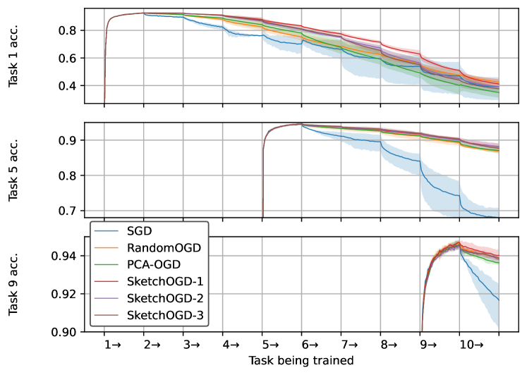
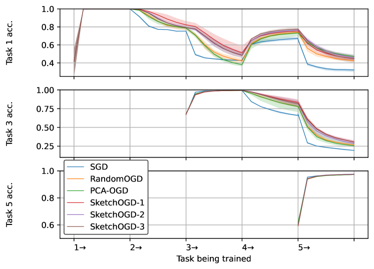
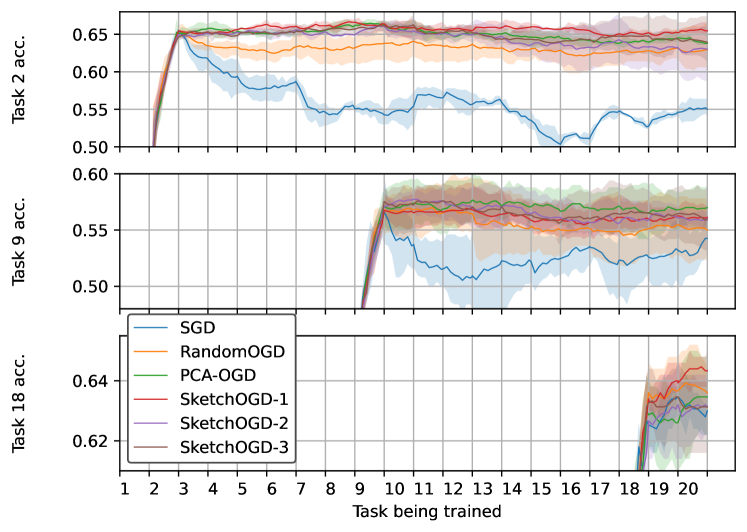
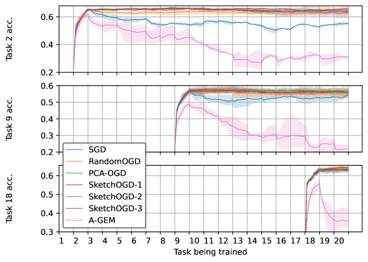
In this section, we provide an extended list of plots for visualizing the experimental results. First, we show the performance of SketchOGD compared to other OGD variants in Rotated MNIST, Permuted MNIST, Split MNIST, and Split CIFAR in Figures 4-7. Then, we also plot A-GEM’s performance on Split CIFAR in Figure 8. A-GEM performs significantly worse in Split CIFAR than any OGD variant, suggesting that the single-gradient approach of A-GEM is ineffective for larger models.

Figure 4: Accuracy of various continual learning methods on tasks 1, 5, and 9 of the Rotated MNIST benchmark. Each plot shows the initial learning of a task and the subsequent slow forgetting as the model trains on new tasks. As shown, SketchOGD-2,3 perform the best in this scenario.

Figure 5: Accuracy of various continual learning methods on tasks 1, 5, and 9 of the Permuted MNIST benchmark. Each plot shows the initial learning of a task and the subsequent slow forgetting as the model trains on new tasks. As shown, SketchOGD-1 performs the best in this scenario. Interestingly, SGD experiences relatively less catastrophic forgetting on the first task compared to later tasks.

Figure 6: Accuracy of various continual learning methods on tasks 1, 3, and 5 of the Split MNIST benchmark. Each plot shows the initial learning of a task and the subsequent slow forgetting as the model trains on new tasks. The OGD variants show similar performance in this scenario while they outperform SGD.

Figure 7: Accuracy of various continual learning methods on tasks 2, 9, and 18 of the Split CIFAR benchmark. Each plot shows the initial learning of a task and the subsequent slow forgetting as the model trains on new tasks. The OGD variants show similar performance in this scenario while they outperform SGD.

Figure 8: Accuracy of various continual learning methods including A-GEM on tasks 2, 9, and 18 of the Split CIFAR benchmark. Each plot shows the initial learning of a task and the subsequent slow forgetting as the model trains on new tasks. As shown, A-GEM experiences significantly more catastrophic forgetting than other methods including SGD.

References

- Barnett and Ceci [2002] Susan M Barnett and Stephen J Ceci. When and where do we apply what we learn?: A taxonomy for far transfer. Psychological bulletin, 2002.
- Bremner et al. [2012] Andrew J Bremner, David J Lewkowicz, and Charles Spence. Multisensory development. Oxford University Press, 2012.
- McCloskey and Cohen [1989] Michael McCloskey and Neal J. Cohen. Catastrophic interference in connectionist networks: The sequential learning problem. Psychology of Learning and Motivation, 1989.
- Farajtabar et al. [2019] Mehrdad Farajtabar, Navid Azizan, Alexander Mott, and Ang Li. Orthogonal gradient descent for continual learning. In International Conference on Artificial Intelligence and Statistics, 2019.
- Li and Liang [2018] Yuanzhi Li and Yingyu Liang. Learning overparameterized neural networks via stochastic gradient descent on structured data. Advances in neural information processing systems, 2018.
- Azizan and Hassibi [2019] Navid Azizan and Babak Hassibi. Stochastic gradient/mirror descent: Minimax optimality and implicit regularization. In International Conference on Learning Representations, 2019.
- Azizan et al. [2022] Navid Azizan, Sahin Lale, and Babak Hassibi. Stochastic mirror descent on overparameterized nonlinear models. IEEE Transactions on Neural Networks and Learning Systems, 2022.
- Allen-Zhu et al. [2019] Zeyuan Allen-Zhu, Yuanzhi Li, and Zhao Song. A convergence theory for deep learning via over-parameterization. In International Conference on Machine Learning, 2019.
- Chaudhry et al. [2019] Arslan Chaudhry, Marc’Aurelio Ranzato, Marcus Rohrbach, and Mohamed Elhoseiny. Efficient lifelong learning with A-GEM. In International Conference on Learning Representations, 2019.
- Tropp et al. [2017] Joel A. Tropp, Alp Yurtsever, Madeleine Udell, and Volkan Cevher. Practical sketching algorithms for low-rank matrix approximation. SIAM Journal on Matrix Analysis and Applications, 2017.
- Ratcliff [1990] Roger Ratcliff. Connectionist models of recognition memory: Constraints imposed by learning and forgetting functions. Psychological Review, 1990.
- Robins [1995] Anthony Robins. Catastrophic forgetting, rehearsal and pseudorehearsal. Connection Science, 1995.
- Shin et al. [2017] Hanul Shin, Jung Kwon Lee, Jaehong Kim, and Jiwon Kim. Continual learning with deep generative replay. In Neural Information Processing Systems, 2017.
- Rebuffi et al. [2017] Sylvestre-Alvise Rebuffi, Alexander Kolesnikov, Georg Sperl, and Christoph H Lampert. icarl: Incremental classifier and representation learning. In Proceedings of the IEEE conference on Computer Vision and Pattern Recognition, 2017.
- Rolnick et al. [2019] David Rolnick, Arun Ahuja, Jonathan Schwarz, Timothy Lillicrap, and Gregory Wayne. Experience replay for continual learning. Neural Information Processing Systems, 2019.
- Van de Ven et al. [2020] Gido M Van de Ven, Hava T Siegelmann, and Andreas S Tolias. Brain-inspired replay for continual learning with artificial neural networks. Nature Communications, 2020.
- Pellegrini et al. [2020] Lorenzo Pellegrini, Gabriele Graffieti, Vincenzo Lomonaco, and Davide Maltoni. Latent replay for real-time continual learning. In 2020 IEEE/RSJ International Conference on Intelligent Robots and Systems (IROS), 2020.
- Rusu et al. [2016] Andrei A. Rusu, Neil C. Rabinowitz, Guillaume Desjardins, Hubert Soyer, James Kirkpatrick, Koray Kavukcuoglu, Razvan Pascanu, and Raia Hadsell. Progressive neural networks. arXiv:1606.04671, 2016.
- Valkov et al. [2018] Lazar Valkov, Dipak Chaudhari, Akash Srivastava, Charles Sutton, and Swarat Chaudhuri. Houdini: Lifelong learning as program synthesis. Advances in neural information processing systems, 2018.
- Veniat et al. [2021] Tom Veniat, Ludovic Denoyer, and MarcAurelio Ranzato. Efficient continual learning with modular networks and task-driven priors. In International Conference on Learning Representations, 2021.
- Ostapenko et al. [2021] Oleksiy Ostapenko, Pau Rodriguez, Massimo Caccia, and Laurent Charlin. Continual learning via local module composition. Neural Information Processing Systems, 2021.
- Kirkpatrick et al. [2016] James Kirkpatrick, Razvan Pascanu, Neil C. Rabinowitz, Joel Veness, Guillaume Desjardins, Andrei A. Rusu, Kieran Milan, John Quan, Tiago Ramalho, Agnieszka Grabska-Barwinska, Demis Hassabis, Claudia Clopath, Dharshan Kumaran, and Raia Hadsell. Overcoming catastrophic forgetting in neural networks. Proceedings of the National Academy of Sciences, 2016.
- Zenke et al. [2017] Friedemann Zenke, Ben Poole, and Surya Ganguli. Continual learning through synaptic intelligence. International Conference on Machine Learning, 2017.
- Parisi et al. [2019] German I. Parisi, Ronald Kemker, Jose L. Part, Christopher Kanan, and Stefan Wermter. Continual lifelong learning with neural networks: A review. Neural Networks, 2019.
- Min et al. [2022] Youngjae Min, Kwangjun Ahn, and Navid Azizan. One-pass learning via bridging orthogonal gradient descent and recursive least-squares. In Conference on Decision and Control, 2022.
- Achlioptas and McSherry [2007] Dimitris Achlioptas and Frank McSherry. Fast computation of low-rank matrix approximations. Journal of the ACM, 2007.
- de Hoog and Mattheij [2007] F.R. de Hoog and R.M.M. Mattheij. Subset selection for matrices. Linear Algebra and its Applications, 2007.
- Halko et al. [2011] N. Halko, P. G. Martinsson, and J. A. Tropp. Finding structure with randomness: Probabilistic algorithms for constructing approximate matrix decompositions. SIAM Review, 2011.
- Cheng et al. [2005] H. Cheng, Z. Gimbutas, P. G. Martinsson, and V. Rokhlin. On the compression of low rank matrices. SIAM Journal on Scientific Computing, 2005.
- Sharma et al. [2021] Apoorva Sharma, Navid Azizan, and Marco Pavone. Sketching curvature for efficient out-of-distribution detection for deep neural networks. In Uncertainty in Artificial Intelligence, 2021.
- Doan et al. [2020] Thang Van Doan, Mehdi Abbana Bennani, Bogdan Mazoure, Guillaume Rabusseau, and Pierre Alquier. A theoretical analysis of catastrophic forgetting through the NTK overlap matrix. In International Conference on Artificial Intelligence and Statistics, 2020.
- Ye and Lim [2016] Ke Ye and Lek-Heng Lim. Schubert varieties and distances between subspaces of different dimensions. SIAM Journal on Matrix Analysis and Applications, 2016.
- Reuther et al. [2018] Albert Reuther, Jeremy Kepner, Chansup Byun, Siddharth Samsi, William Arcand, David Bestor, Bill Bergeron, Vijay Gadepally, Michael Houle, Matthew Hubbell, Michael Jones, Anna Klein, Lauren Milechin, Julia Mullen, Andrew Prout, Antonio Rosa, Charles Yee, and Peter Michaleas. Interactive supercomputing on 40,000 cores for machine learning and data analysis. In 2018 IEEE High Performance extreme Computing Conference (HPEC), 2018.
- Muirhead [1982] R.J. Muirhead. Aspects of Multivariate Statistical Theory. Wiley, 1982.