Performance-Robustness Tradeoffs in Adversarially Robust Control and Estimation

Abstract

While $\mathcal{H}_{\infty}$ methods can introduce robustness against worst-case perturbations, their nominal performance under conventional stochastic disturbances is often drastically reduced. Though this fundamental tradeoff between nominal performance and robustness is known to exist, it is not well-characterized in quantitative terms. Toward addressing this issue, we borrow the increasingly ubiquitous notion of adversarial training from machine learning to construct a class of controllers which are optimized for disturbances consisting of mixed stochastic and worst-case components. We find that this problem admits a linear time invariant optimal controller that has a form closely related to suboptimal $\mathcal{H}_{\infty}$ solutions. We then provide a quantitative performance-robustness tradeoff analysis in two analytically tractable cases: state feedback control, and state estimation. In these special cases, we demonstrate that the severity of the tradeoff depends in an interpretable manner upon system-theoretic properties such as the spectrum of the controllability gramian, the spectrum of the observability gramian, and the stability of the system. This provides practitioners with general guidance for determining how much robustness to incorporate based on a priori system knowledge. We empirically validate our results by comparing the performance of our controller against standard baselines, and plotting tradeoff curves.

1 Introduction

Modern control systems, from mobile robotics to power plants, require controllers that are simultaneously fast, performant, and robust. Many control schemes attempt to achieve these desiderata by combining them into a single objective function and optimizing it, leading to a natural tradeoff. A controller optimized for speed and efficiency may perform poorly in the face of unmodeled phenomena. For instance, Linear-Quadratic Gaussian (LQG) controllers (a special case of $\mathcal{H}_{2}$ controllers) explicitly prioritize nominal performance by penalizing the expectation of a quadratic function of the state and input. However, such controllers can be arbitrarily fragile to small perturbations of the dynamics (Doyle, 1978). Replacing the LQG objective with one that considers the response of the system to worst-case dynamic uncertainty and external disturbances results in robust control methods, such as $\mathcal{H}_{\infty}$ and $\mathcal{L}_{1}$ methods Zhou et al. (1996); Dahleh and Diaz-Bobillo (1994). Such controllers are provably robust, however they tend to be overly conservative in practice.

Toward balancing the performance of nominal and robust controllers, various approaches have been introduced, most notably mixed $\mathcal{H}_{2}/\mathcal{H}_{\infty}$ methods. However, the resulting controllers are often complicated to express and compute (Scherer, 1995), and lack a quantitative characterization of the tradeoff between performance and robustness as a function of system properties. Toward addressing these issues, we take inspiration from the notion of adversarial robustness from machine learning (Biggio et al., 2013; Goodfellow et al., 2014; Madry et al., 2017; Carlini and Wagner, 2017) and formulate a controller synthesis problem that balances performance and robustness. The goal of adversarial robustness in machine learning is to minimize the expected error under the presence of worst-case norm-bounded perturbations to the data, where the perturbations can depend on the underlying stochasticity of the problem, such as the data distribution and additive noise. We consider an analogous adversarially robust output feedback control problem where we aim to minimize an expected quadratic cost subject to linear dynamics driven by process noise composed of two components: a zero-mean stochastic noise term and a norm-bounded adversarial term. We show that the solution to this problem may be expressed in terms of the solutions to a set of coupled Discrete Algebraic Riccati equations (DAREs). For several special cases, this allows for novel quantitative performance-robustness tradeoff bounds to be computed in which system parameters manifest in an interpretable way.

1.1 Contributions

Toward analyzing the adversarially robust control problem we propose, we first show that when viewed through the lens of dynamic games (Basar, 1991), adversarially robust LQ control relates to a control problem introduced in Doyle et al. (1989b). We show that the optimal solution to the state feedback version of this problem is given by a central static suboptimal $\mathcal{H}_{\infty}$ controller, with suboptimality level $\gamma$ depending on both the stochastic noise statistics and the budget given to the adversary. Furthermore, both the worst-case adversary and the corresponding optimal controller can be computed from the solution of a DARE. We then leverage the state feedback solution to provide sufficient conditions for a solution to the output feedback control problem, along with an algorithm to synthesize this controller. Unlike the state feedback setting, the output feedback adversarially robust controller is distinct from a central suboptimal $\mathcal{H}_{\infty}$ controller, and involves finding the solution to a set of coupled Riccati equations.

We leverage the solution to the adversarially robust control problem to quantify the performance-robustness tradeoffs analytically in two simplified settings: state feedback LQ control, and state estimation. In these settings, we show an interpretable dependence on underlying system-theoretic properties such as controllability, observability, and stability. For the state feedback control setting, we show that the cost gap incurred by the adversarially robust controller in the nominal setting, relative to that achieved by the nominal controller, is upper bounded by $O(\sigma_{w}^{2}\gamma^{-4}\nu^{-1})$. In this expression, $\sigma_{w}^{2}$ is the covariance of the additive noise distribution, $\gamma$ is the suboptimality level of the suboptimal $\mathcal{H}_{\infty}$ controller, and $\nu$ is the smallest singular value of the controllability gramian. On the other hand, the cost gap is lower bounded by $\Omega\mathopen{}\left(\sigma_{w}^{2}\gamma^{-4}\eta^{2}\right)\mathclose{}$, where $\eta$ is the largest singular value of the controllability gramian for closed-loop system under the nominal LQ controller with disturbances as the input. These results quantitatively show that systems with uniformly good controllability have small performance-robustness tradeoffs, while those that have a highly controllable mode in the nominal closed-loop system (when viewing disturbances as inputs) lead to large performance-robustness tradeoffs. Similar bounds are shown for the state estimation setting, with controllability gramians replaced by observability gramians.

We conclude with numerical experiments. These simulations indicate that the proposed algorithm for synthesizing the controller is effective, and that the controller performs well relative to standard baselines in stabilizing an inverted pendulum. We additionally illustrate that the analytical trends described above are present in numerical experiments. We demonstrate that in the setting of output feedback control, the impact of poor controllability and poor observability compound to increase the severity of the performance-robustness tradeoff.

1.2 Related Work

The mixed stochastic/worst-case problem that we consider is not the only way to strike a balance between the performance of stochastic and robust control methods. Most closely related is Doyle et al. (1989b), which considers a similar problem from a deterministic perspective, in which disturbances are composed of both a bounded power component, and a bounded power spectrum component. A set description of disturbances that also interpolates between $\mathcal{H}_{2}$ and $\mathcal{H}_{\infty}$ approaches is proposed in Paganini (1993). The class of all stabilizing controllers subject to a $\mathcal{H}_{\infty}$ norm constraint is characterized in Glover and Doyle (1988), while minimizing an $\mathcal{H}_{2}$ objective subject to a $\mathcal{H}_{\infty}$ constraint is addressed in Bernstein and Haddad (1988); Rotea and Khargonekar (1991). While conceptually appealing, these methods often lack a simple closed-form stationary solution. A solution to risk-sensitive LQG control which interpolates between $\mathcal{H}_{2}$ and $\mathcal{H}_{\infty}$ solutions is offered in in Whittle (1981). Other recent work also attempts to reduce the conservatism of robust control through risk aware approaches (Tsiamis et al., 2021; Chapman and Lessard, 2022) or regret-minimization (Goel and Hassibi, 2020, 2021; Hazan et al., 2020). None of the aforementioned methods characterize the performance-robustness tradeoffs of the resulting controllers.

Analogous recent work in the machine learning community has analyzed performance-robustness tradeoffs in adversarially robust learning, including precise characterizations of the generalization errors of standard versus adversarially trained models under various theoretical assumptions (Zhang et al., 2019; Javanmard et al., 2020; Hassani and Javanmard, 2022), and “no free lunch” theorems for obtaining adversarially robust models (Tsipras et al., 2018; Dohmatob, 2019; Yin et al., 2019). The successful characterization of such performance-robustness tradeoffs in machine learning motivates the control objective we consider. However, the theoretical results from this area are largely intended for the supervised learning setting and do not immediately apply to our setting. The existence of performance-robustness tradeoffs in control is shown in Al Makdah et al. (2020), but they are not characterized quantitatively. Our prior work studies performance robustness tradeoffs in the setting of state feedback control (Lee et al., 2022) and finite horizon state estimation (Zhang et al., 2021). This paper expands upon these works to consider performance robustness tradeoffs of both control and state estimation in a unified framework by considering them both as special cases of adversarially robust output feedback control. We end by noting that the extension of adversarial robustness results in machine learning to various control problems has recently received attention (Zhang et al., 2022; Havens et al., 2022; Pattanaik et al., 2017; Tan et al., 2020; Mandlekar et al., 2017; Kuutti et al., 2021).

Notation: The Euclidean norm of a vector $x$ is denoted by $\left\|x\right\|$. For a matrix $A$, the spectral norm is denoted $\left\|A\right\|$ and the Frobenius norm is denoted $\left\|A\right\|_{F}$. The spectral radius of a square matrix $A$ is denoted $\rho(A)$. A symmetric, positive semidefinite (psd) matrix $A=A^{\top}$ is denoted $A\succeq 0$, and a symmetric positive definite (pd) matrix is denoted $A\succ 0$. Similarly $A\succeq B$ denotes that $A-B$ is positive semidefinite. A sequence of vectors $x_{t}$ defined for $t\geq 0$ will be denoted by $\mathbf{x}=\mathopen{}\left\{x_{t}\right\}\mathclose{}_{t\geq 0}$. The $\ell^{2}$ signal-norm of a sequence is denoted by $\left\|\mathbf{x}\right\|_{\ell^{2}}:=(\sum_{t\geq 0}\left\|x_{t}\right\|^{2})^{1/2}$. For an autonomous system $x_{t+1}=Ax_{t}$ and symmetric matrix $Q$, we denote the solution $P$ to the discrete Lyapunov equation

$$A^{\top}PA-P+Q=0$$

by $\textnormal{{dlyap}}(A,Q)$. Similarly, for a controlled system $x_{t+1}=Ax_{t}+Bu_{t}$ and symmetric matrices $Q,R$ of compatible size, we denote the solution $P$ to the discrete algebraic Riccati equation

$$Q+A^{\top}PA-A^{\top}PB(B^{\top}PB+R)^{-1}B^{\top}PA=P$$

by $\textnormal{{DARE}}(A,B,Q,R)$.

2 Adversarially Robust Linear-Quadratic Control

Consider a partially observed discrete-time linear-time-invariant (LTI) system with state and measurement disturbances composed of both stochastic and adversarial components: let $x_{t}\in\mathbb{R}^{n_{x}}$ be the system state, $u_{t}\in\mathbb{R}^{n_{u}}$ the input, $y_{t}\in\mathbb{R}^{n_{y}}$ the measurement, $w_{t}\in\mathbb{R}^{n_{w}}$ and $\delta_{t}\in\mathbb{R}^{n_{\delta}}$ the stochastic and adversarial components of the process disturbance, respectively. The initial condition $x_{0}$ and stochastic component of the process noise $w_{t}$ are assumed to be i.i.d. zero-mean with covariance matrices $\Sigma_{0},\;I$, respectively, and $\mathbb{E}\mathopen{}\left[x_{0}w_{t}^{\top}\right]\mathclose{}=0$ for all $t\geq 0$. The performance will be measured by an output signal $z_{t}\in\mathbb{R}^{n_{z}}$ which depends on the current state and input. The LTI system is then defined by the following equations:

$$x_{t+1} =Ax_{t}+B_{0}w_{t}+B_{1}\delta_{t}+B_{2}u_{t}$$ (1)

$$z_{t} =C_{1}x_{t}+D_{12}u_{t}$$

$$y_{t} =C_{2}x_{t}+D_{20}w_{t}+D_{21}\delta_{t}.$$

We denote this system compactly by

$$G=\left[\begin{array}[]{c|ccc}A&B_{0}&B_{1}&B_{2}\\ \hline\cr C_{1}&D_{10}&0&D_{12}\\ C_{2}&D_{20}&D_{21}&0\end{array}\right],$$

and adopt the notation $\mathcal{F}_{l}(G,K)$ to denote its feedback interconnection with a controller $K$ that takes the signal $y_{t}$ as input, and outputs control action $u_{t}$.

We assume that the adversarial perturbation sequence $\bm{\delta}$ is causal, i.e., it can depend only on the states, inputs, and stochastic noise up to the current timestep; in particular, $\delta_{t}$ must be a measurable function of the randomness $x_{0},w_{0:t}$. We consider the infinite horizon objective defined in terms of the performance signal

$$\limsup_{T\to\infty}\frac{1}{T}\mathbb{E}_{\mathbf{w},x_{0}}\mathopen{}\left[\sum_{t=0}^{T-1}\left\|z_{t}\right\|^{2}\right]\mathclose{},$$ (2)

subject to the dynamics (1). We assume that $C_{1}=\begin{bmatrix}Q^{1/2}\\ 0\end{bmatrix}$ and $D_{12}=\begin{bmatrix}0\\ R^{1/2}\end{bmatrix}$ for $Q\succeq 0$, and $R\succ 0$, so that (2) reduces to the linear quadratic regulation cost. Therefore, if the adversarial perturbations $\bm{\delta}$ are set to zero, then the system (1) with objective (2) forms the nominal Linear Quadratic Gaussian (LQG) problem. If the stochasticity is set to zero ($\bm{w},x_{0}=0$) and $\bm{\delta}$ are worst-case perturbations with average power bounded by $\varepsilon$, then we instead recover the $\mathcal{H}_{\infty}$ problem. When both stochastic noise and worst-case perturbations are present, we define the resulting control task as the adversarially robust LQG problem. We denote the three corresponding objectives by nominal cost ($\operatorname{NC}$), robust cost ($\operatorname{RC}$), and adversarial cost ($\operatorname{AC}$) respectively:

$$\operatorname{NC}(K) =\limsup_{T\to\infty}\frac{1}{T}\mathbb{E}_{\mathbf{w},x_{0}}\mathopen{}\left[\sum_{t=0}^{T-1}\left\|z_{t}\right\|^{2}\right]\mathclose{},\;\;\bm{\delta}=0,$$ (3)

$$\operatorname{RC}(K) =\limsup_{T\to\infty}\frac{1}{T}\max_{\begin{subarray}{c}\bm{\delta}\mbox{ causal}\\ \left\|\bm{\delta}\right\|_{\ell_{2}}^{2}\leq T\varepsilon\end{subarray}}\sum_{t=0}^{T-1}\left\|z_{t}\right\|^{2},\;\;\begin{bmatrix}x_{0}\\ \bm{w}\end{bmatrix}=0,$$ (4)

$$\operatorname{AC}(K) =\limsup_{T\to\infty}\frac{1}{T}\mathbb{E}_{\mathbf{w},x_{0}}\mathopen{}\left[\max_{\begin{subarray}{c}\bm{\delta}\mbox{ causal}\\ \left\|\bm{\delta}\right\|_{\ell_{2}}^{2}\leq T\varepsilon\end{subarray}}\sum_{t=0}^{T-1}\left\|z_{t}\right\|^{2}\right]\mathclose{}.$$ (5)

The constraint $\left\|\bm{\delta}\right\|_{\ell^{2}}^{2}\leq T\varepsilon$ is chosen such that the instance-wise adversarial budget satisfies $\left\|\delta_{t}\right\|^{2}\leq\varepsilon$ on average. In order to ensure that there exists a stabilizing controller, and that minimizing either $\operatorname{NC}$ or $\operatorname{RC}$ provides a stabilizing controller, we make the following standard assumption (Zhou et al., 1996).

Assumption 2.1

 

• $(A,B_{2},C_{2})$ is stabilizable and detectable.

• $(A,Q^{1/2})$ is detectable.

• $R\succ 0$, $B_{0}B_{0}^{\top}\succ 0$, $D_{20}D_{20}^{\top}\succ 0$, $B_{0}D_{20}^{\top}=0$.

Under this assumption, there exists a stabilizing controller minimizing $\operatorname{NC}$, of the form

$$\hat{x}_{t} =(A+B_{2}F_{\star})(I-L_{\star}C_{2})\hat{x}_{t}+(A+B_{2}F_{\star})L_{\star}y_{t}$$

$$u_{t} =F_{\star}(I-L_{\star}C_{2})\hat{x}_{t}+F_{\star}L_{\star}y_{t},$$

where

$$F_{\star} =-(R+B_{2}^{\top}P_{\star}B_{2})^{-1}B_{2}^{\top}P_{\star}A$$ (6)

$$L_{\star} =\Sigma_{\star}C_{2}^{\top}(C_{2}\Sigma_{\star}C_{2}^{\top}+D_{20}D_{20})^{-1},$$ (7)

and $P_{\star}$ and $\Sigma_{\star}$ solve the following two Discrete Algebraic Riccati Equations (DARE):

$$P_{\star} =\textnormal{{DARE}}(A,B,Q,R)$$ (8)

$$\Sigma_{\star} =\textnormal{{DARE}}(A^{\top},C^{\top},B_{0}B_{0}^{\top},D_{20}D_{20}^{\top}).$$ (9)

The above solution is called the LQG controller. A solution minimizing $\operatorname{RC}$ is known as an $\mathcal{H}_{\infty}$ controller, and may be expressed in terms of the solution to two modified DAREs Basar (1991); Hassibi et al. (1999).

The remainder of this section is devoted to finding a controller minimizing $\operatorname{AC}$. Inspired by minimax dynamic games (Basar, 1991), we first find a controller which minimizes a soft-constrained version of the adversarial cost (5):

$$\limsup_{T\to\infty}\frac{1}{T}\mathbb{E}\mathopen{}\left[\max_{\bm{\delta}\mbox{ causal}}\sum_{t=0}^{T-1}\left\|z_{t}\right\|^{2}-\gamma^{2}\left\|\delta_{t}\right\|^{2}\right]\mathclose{}.$$ (10)

The following lemma provides necessary and sufficient conditions for the existence of a stabilizing controller which minimizes the above objective in the state feedback setting ($C_{2}=I$, $D_{20}=0$, and $D_{21}=0$.) Similar statements in continuous time may be extracted from a result found in Doyle et al. (1989b).

Lemma 2.1

Suppose there exists a solution to the following DARE

$$P_{\gamma}=\textnormal{{DARE}}\mathopen{}\left(A,\begin{bmatrix}B_{1}&B_{2}\end{bmatrix},Q,\begin{bmatrix}-\gamma^{2}I\\ &R\end{bmatrix}\right)\mathclose{}$$ (11)

satisfying $P_{\gamma}\succeq 0$ and $B_{1}^{\top}P_{\gamma}B_{1}\prec\gamma^{2}I$. When the above condition holds,

1. Let

   $$\Psi=\begin{bmatrix}B_{1}&B_{2}\end{bmatrix}^{\top}P_{\gamma}\begin{bmatrix}B_{1}&B_{2}\end{bmatrix}+\begin{bmatrix}-\gamma^{2}I&0\\ 0&R\end{bmatrix}.$$ (12)

   Then the controller $u_{t}=F_{\gamma}x_{t}$ with $F_{\gamma}$ given by

   $$\begin{bmatrix}E_{\gamma}\\ F_{\gamma}\end{bmatrix}:=-\Psi^{-1}\begin{bmatrix}B_{1}&B_{2}\end{bmatrix}^{\top}PA$$ (13)

   satisfies $\rho(A+B_{2}K)<1$, and minimizes objective (10).

2. The optimal adversarial perturbation under the controller $u_{t}=F_{\gamma}x_{t}$ is given by

   $$\Delta_{\gamma} =(\gamma^{2}I-B_{1}^{\top}PB_{1})^{-1}B_{1}^{\top}PB_{0},$$ (14)

   $$\delta_{t} =E_{\gamma}x_{t}+\Delta_{\gamma}w_{t}.$$

3. The objective value (10) achieved under controller (13) and adversary (14) is $\operatorname{Tr}(M_{\gamma}B_{0}B_{0}^{\top})$, where $M_{\gamma}=P_{\gamma}+P_{\gamma}B_{1}(\gamma^{2}I-B_{1}^{\top}P_{\gamma}B_{1})^{-1}B_{1}^{\top}P_{\gamma}$.

The solution approach for the above problem follows that in Basar (1991) for minimax games. The finite horizon version of the problem is solved by defining a saddle point cost-to-go, then recursing backwards in time, solving both an unconstrained concave maximization problem and convex minimization problem at each time step to determine the optimal adversarial perturbation and control input. The causality of $\bm{\delta}$ is necessary in the recursion to pull $\delta_{t}$ out of an expectation over future noise terms. Taking the limit as the horizon tends to infinity provides the steady state controller and adversary in the above lemma statement. See Appendix A.1 for the proof. It should be noted that in contrast to most adversarially robust machine learning problems, adversarially robust LQR provides a closed-form expression for the adversarial perturbation.

We now leverage the state feedback solution to solve the soft-constrained output feedback problem.

Lemma 2.2

Suppose that

1. There exists a solution to the following DARE

   $$P_{\gamma}=\textnormal{{DARE}}\mathopen{}\left(A,\begin{bmatrix}B_{1}&B_{2}\end{bmatrix},Q,\begin{bmatrix}-\gamma^{2}I\\ &R\end{bmatrix}\right)\mathclose{}$$

   satisfying $P_{\gamma}\succeq 0$ and $B_{1}^{\top}P_{\gamma}B_{1}\prec\gamma^{2}I$. Let $F_{\gamma}$, $E_{\gamma}$ and $\Delta_{\gamma}$ be the corresponding gains from Lemma 2.1. Also let $\Psi$ be as in (12).

2. There exists a nonsingular matrix $\begin{bmatrix}\hat{T}_{11}&0\\ \hat{T}_{21}&\hat{T}_{22}\end{bmatrix}$ with $\hat{T}_{11}\in\mathbb{R}^{n_{\delta}\times n_{\delta}}$, and $\hat{T}_{22}\in\mathbb{R}^{n_{u}\times n_{u}}$ such that

   $$\Psi=\begin{bmatrix}\hat{T}_{11}&0\\ \hat{T}_{21}&\hat{T}_{22}\end{bmatrix}^{\top}\begin{bmatrix}-I\\ &I\end{bmatrix}\begin{bmatrix}\hat{T}_{11}&0\\ \hat{T}_{21}&\hat{T}_{22}\end{bmatrix}.$$ (15)

3. There exists real matrices $L_{\gamma},N_{\gamma},\Sigma_{\gamma},Y_{\gamma}$, where $\Sigma_{\gamma},Y_{\gamma}\succ 0$, that satisfy

   $$\tilde{A} =\hat{A}+L_{\gamma}\hat{C}_{2},$$ (16)

   $$\tilde{B}_{0} =\hat{B}_{0}+L_{\gamma}\hat{D}_{20},$$

   $$\tilde{B}_{1} =\hat{B}_{1}+L_{\gamma}\hat{D}_{21}$$

   $$\tilde{C}_{1} =\hat{C}_{1}+N_{\gamma}\hat{C}_{2}$$

   $$\tilde{D}_{11} =\hat{D}_{11}+N_{\gamma}\hat{D}_{21}$$

   $$\tilde{D}_{10} =N_{\gamma}\hat{D}_{20}$$

   $$\Phi =I-\tilde{D}_{11}^{\top}\tilde{D}_{11}-\tilde{B}_{1}^{\top}Y_{\gamma}\tilde{B}_{1}\succ 0$$

   $$Y_{\gamma} =\tilde{C}_{1}^{\top}\tilde{C}_{1}+\tilde{A}^{\top}Y_{\gamma}\tilde{A}+\mathopen{}\left(\tilde{D}_{11}^{\top}\tilde{C}_{1}+\tilde{B}_{1}^{\top}Y_{\gamma}\tilde{A}\right)\mathclose{}^{\top}\Phi^{-1}\mathopen{}\left(\tilde{D}_{11}^{\top}\tilde{C}_{1}+\tilde{B}_{1}^{\top}Y_{\gamma}\tilde{A}\right)\mathclose{}$$

   $$\Sigma_{\gamma} =\mathopen{}\left[(I+\tilde{B}_{1}\Phi^{-1}\tilde{B}_{1}^{\top}Y_{\gamma})\tilde{A}+\tilde{B}_{1}\Phi^{-1}\tilde{D}_{11}^{\top}\tilde{C}_{1}\right]\mathclose{}\Sigma_{\gamma}\mathopen{}\left[(I+\tilde{B}_{1}\Phi^{-1}\tilde{B}_{1}^{\top}Y_{\gamma})\tilde{A}+\tilde{B}_{1}\Phi^{-1}\tilde{D}_{11}^{\top}\tilde{C}_{1}\right]\mathclose{}^{\top}$$

   $$\qquad+\mathopen{}\left[(I+\tilde{B}_{1}\Phi^{-1}\tilde{B}_{1}^{\top}Y_{\gamma})\tilde{B}_{0}+\tilde{B}_{1}^{\top}\Phi^{-1}\tilde{D}_{11}^{\top}\tilde{D}_{10}\right]\mathclose{}\mathopen{}\left[(I+\tilde{B}_{1}\Phi^{-1}\tilde{B}_{1}^{\top}Y_{\gamma})\tilde{B}_{0}+\tilde{B}_{1}^{\top}\Phi^{-1}\tilde{D}_{11}^{\top}\tilde{D}_{10}\right]\mathclose{}^{\top}$$

   $$L_{\gamma}, N_{\gamma}\in\operatorname*{argmin}_{L,N}\operatorname{Tr}\mathopen{}\left(\tilde{D}_{10}^{\top}\tilde{D}_{10}+\tilde{B}_{0}^{\top}Y_{\gamma}\tilde{B}_{0}+(\tilde{D}_{10}^{\top}\tilde{D}_{11}+\tilde{B}_{0}^{\top}Y_{\gamma}\tilde{B}_{1})\Phi^{-1}(\tilde{D}_{10}^{\top}\tilde{D}_{11}+\tilde{B}_{0}^{\top}Y_{\gamma}\tilde{B}_{1})^{\top}\right)\mathclose{}$$

   $$\qquad\qquad+\operatorname{Tr}\mathopen{}\left(\Sigma_{\gamma}\mathopen{}\left[\tilde{C}_{1}^{\top}\tilde{C}_{1}+\tilde{A}^{\top}Y_{\gamma}\tilde{A}+(\tilde{D}_{11}^{\top}\tilde{C}_{1}+\tilde{B}_{1}^{\top}Y_{\gamma}\tilde{A})^{\top}\Phi^{-1}(\tilde{D}_{11}^{\top}\tilde{C}_{1}+\tilde{B}_{1}^{\top}Y_{\gamma}\tilde{A})\right]\mathclose{}\right)\mathclose{},$$

   where $Y_{\gamma}$ and $\Sigma_{\gamma}$ are treated as fixed parameters in the minimization problem in the final lines, and

   $$\hat{G}=\left[\begin{array}[]{c|ccc}\hat{A}&\hat{B}_{0}&\hat{B}_{1}&\hat{B}_{2}\\ \hline\cr\hat{C}_{1}&0&\hat{D}_{11}&I\\ \hat{C}_{2}&\hat{D}_{20}&\hat{D}_{21}&0\end{array}\right]:=\left[\begin{array}[]{c|ccc}A+B_{1}E_{\gamma}&B_{0}+B_{1}\Delta_{\gamma}&B_{1}\hat{T}_{11}^{-1}&B_{2}\hat{T}_{22}^{-1}\\ \hline\cr-\hat{T}_{22}F_{\gamma}&0&\hat{T}_{21}\hat{T}_{11}^{-1}&I\\ C_{2}+D_{21}E_{\gamma}&D_{20}+D_{21}\Delta_{\gamma}&D_{21}\hat{T}_{11}^{-1}&0\end{array}\right].$$ (23)

When the above conditions hold, the controller

$$K=\left[\begin{array}[]{c| cc}\hat{A}-\hat{B}_{2}(\hat{C}_{1}+N_{\gamma}\hat{C}_{2})+L_{\gamma}\hat{C}_{2}&L_{\gamma}-\hat{B}_{2}N_{\gamma}\\ \hline\cr\hat{T}_{22}^{-1}(\hat{C}_{1}+N_{\gamma}\hat{C}_{2})&\hat{T}_{22}^{-1}N_{\gamma}\end{array}\right]$$

internally stabilizes the system (1) under the optimal adversarial perturbation and minimizes the objective (10).

The solution approach for the soft-constrained output feedback control synthesis above follows the separation argument outlined in e.g. Doyle et al. (1989a); Zhou et al. (1996); Iglesias and Glover (1991) to reduce the output feedback control problem to that of estimating the optimal state feedback control input from noisy observations of the state. This can in turn be solved via another appeal to the dynamic programming argument from Basar (1991). The main challenge in doing so is that the optimal adversary causes a coupling between the future cost-to-go, and the estimation error-to-arrive. We do not know of existing numerical schemes which provably converge to the optimal $L_{\gamma},N_{\gamma},\Sigma_{\gamma}$ and $Y_{\gamma}$. However, an alternating solution which works well in practice is proposed in Algorithm 1. The proof of Lemma 2.2 can be found in Appendix A.2.

Algorithm 1 Computing Soft-Constrained Adversarially Robust Controller: SoftAdvController$(\hat{G},\gamma,k)$

1:Input: System $\hat{G}$ from (23), soft adversarial penalty $\gamma$, number of iterations $k$.

2:Initialize $L_{\gamma}$ and $N_{\gamma}$ as the Kalman Filter gains for $\hat{G}$

3:for $k$ times do

4:     Given $L_{\gamma}$ and $N_{\gamma}$, compute $Y_{\gamma}$ according to (16), neglecting the final two conditions that $L_{\gamma},N_{\gamma}$ minimize the provided function, and that $\Sigma_{\gamma}$ solves the provided Lyapunov equation.

5:     Given $L_{\gamma}$, $N_{\gamma}$, and $Y_{\gamma}$, compute $\Sigma_{\gamma}$ according to (16), neglecting the final condition that $L_{\gamma},N_{\gamma}$ minimize the provided function.

6:     Given $Y_{\gamma}$ and $\Sigma_{\gamma}$, compute the gains $L_{\gamma}$ and $N_{\gamma}$ according to the final condition in (16), neglecting the Riccati equation for $Y_{\gamma}$ and the Lyapunov equation for $\Sigma_{\gamma}$.

7:end for

8:Output: Gains $L_{\gamma}$, $N_{\gamma}$

We now return our attention to objective (5). It can be shown via strong duality that the hard-constrained problem may be solved by sequentially solving the soft-constrained problem using Lemma 2.2. Note that in contrast to the solution approach to minimize $\operatorname{RC}$, dualizing the constraint in $\operatorname{AC}$ results in an optimal dual variable $\gamma(\varepsilon)$ that is a random variable. Therefore, it is nontrivial to exchange the order of the minimization over the dual variable with the expectation (see Appendix A.3 for details). We propose Algorithm 2 to minimize the adversarial cost (5).

Algorithm 2 Computing Adversarially Robust Controller: AdvControl$(G,\varepsilon,\gamma_{LB},\gamma_{UB},\texttt{tol})$

1:Input: System $G$, adversary budget $\varepsilon>0$, binary search bounds $\gamma_{LB}<\gamma_{UB}$, tolerance tol. 

2:// Do binary search on $\gamma\in[\gamma_{LB},\gamma_{UB}]$ to find optimal adversary with average power $\varepsilon>0$

3:while $\gamma_{UB}-\gamma_{LB}\geq\texttt{tol}$ do

4:     $\gamma=(\gamma_{UB}+\gamma_{LB})/2$

5:     if Conditions $1-3$ of Lemma 2.2 are satsified at level $\gamma$ then

6:         Compute the optimal controller $K$ for system $G$ at level $\gamma$ according to Lemma 2.2.

7:         if $\texttt{AdvPower}(\mathcal{F}_{l}(G,K),\gamma)<\varepsilon$ (computed via Algorithm 3) then

8:              $\gamma_{UB}=\gamma$

9:         else

10:              $\gamma_{LB}=\gamma$

11:         end if

12:     else

13:         $\gamma_{LB}=\gamma$

14:     end if

15:end while

16:Output: Adversarially robust controller $K$, closed-loop system $G_{cl}=\mathcal{F}_{l}(G,K)$

Theorem 2.1

Let $\gamma_{LB}$ be a small positive number such that the conditions of Lemma 2.2 are satisfied for all $\gamma\geq\gamma_{LB}$, and $K_{\gamma_{LB}}$ be the corresponding optimal controller. For any $\varepsilon>0$ such that $\texttt{AdvPower}(\mathcal{F}_{l}(G,K_{\gamma_{LB}}),\gamma_{LB})>\varepsilon$, let $\gamma_{UB}$ be sufficiently large such that the controller $K_{\gamma_{UB}}$ at level $\gamma_{UB}$ satisfies $\texttt{AdvPower}(\mathcal{F}_{l}(G,K_{\gamma_{UB}}),\gamma_{UB})<\varepsilon$. Then the output of Algorithm 2, $[K,G_{cl}]$ = AdvControl$(G,\varepsilon,\gamma_{LB},\gamma_{UB},\textnormal{{tol}})$ satisfies (up to the numerical tolerance)

1. The controller $K$ minimizes $\operatorname{AC}(K)$.

2. The minimum value for the adversarial cost (5) is given by $\operatorname{Tr}(J_{\gamma})+\gamma^{2}\varepsilon$, where

   $$J_{\gamma} =D_{0,cl}^{\top}D_{0,cl}+B_{0,cl}^{\top}P_{\gamma}B_{0,cl}+(D_{1,cl}^{\top}D_{0,cl}+B_{1,cl}^{\top}P_{\gamma}B_{0,cl})^{\top}\Phi^{-1}(D_{1,cl}^{\top}D_{0,cl}+B_{1,cl}^{\top}P_{\gamma}B_{0,cl})$$ (24)

   $$P_{\gamma} =\texttt{DARE}(A_{cl},B_{1,cl},C_{cl}^{\top}C_{cl},-\gamma^{2}I,S=C_{cl}^{\top}D_{1,cl})$$

   $$\Phi =\gamma^{2}I-D_{1,cl}^{\top}D_{1,cl}-B_{1,cl}^{\top}P_{\gamma}B_{1,cl}$$

   $$G_{cl} =\left[\begin{array}[]{c|cc}A_{cl}&B_{0,cl}&B_{1,cl}\\ \hline\cr C_{cl}&D_{0,cl}&D_{1,cl}\end{array}\right].$$

   Here, $\textnormal{{DARE}}(A,B,Q,R,S)$ is overloaded to denote the solution $P$ to the generalized DARE,

   $$P =Q+A^{\top}PA+(A^{\top}PB+S)(B^{\top}PB+R)^{-1}(B^{\top}PA+S^{\top}).$$

We observe from Theorem 2.1 that while the LQG controller is independent of the noise statistics, the adversarially robust controller output by Algorithm 2 depends on the noise statistics through the optimal choice of $\gamma$.

In the subsequent sections, we examine the tradeoff in the objective values from minimizing either the nominal objective or the adversarially robust objective. This motivates the following two results, which allow us to compute the nominal and adversarial costs for an arbitrary LTI controller $K$.

Proposition 2.1

For an LTI controller $K$, let $A_{cl}$, $B_{cl}$, $C_{cl}$ and $D_{cl}$ be a state space realization for $\mathcal{F}_{l}(G,K)$. If $\rho(A_{cl})<1$, then the nominal cost may be expressed as

$$\operatorname{NC}(K)=\limsup_{T}\frac{1}{T}\mathbb{E}_{w}\mathopen{}\left[\sum_{t=0}^{T-1}\left\|z_{t}\right\|^{2}\right]\mathclose{}=\operatorname{Tr}\mathopen{}\left(C_{cl}\Sigma_{cl}C_{cl}^{\top}+D_{cl}D_{cl}^{\top}\right)\mathclose{},$$

where $\Sigma_{cl}=A_{cl}\Sigma_{cl}A_{cl}^{\top}+B_{cl}B_{cl}^{\top}.$

Algorithm 3 Computing Adversarially Power: AdvPower$(G_{cl},\gamma)$

1:Input: Closed-loop system $G_{cl}$, adversary penalty $\gamma$.

2:Determine a state space realization for the closed-loop system $\left[\begin{array}[]{c|cc}A_{cl}&B_{0,cl}&B_{1,cl}\\ \hline\cr C_{cl}&D_{0,cl}&D_{1,cl}\end{array}\right]=G_{cl}$.

3:Set $P_{\gamma}=\texttt{DARE}(A_{cl},B_{1,cl},C_{cl}^{\top}C_{cl},-\gamma^{2}I,S=C_{cl}^{\top}D_{1,cl})$.

4:Let $\Phi=\gamma^{2}I-B_{1,cl}^{\top}P_{\gamma}B_{1,cl}$.

5:Let $\Gamma_{x}=D_{1,cl}^{\top}C_{cl}+B_{1,cl}^{\top}P_{\gamma}A_{cl}$, $\Gamma_{w}=D_{1,cl}^{\top}D_{0,cl}+B_{1,cl}^{\top}P_{\gamma}B_{0,cl}$.

6:Assign $\Sigma_{\gamma}=\texttt{dlyap}(A_{cl}+B_{1,cl}\Phi^{-1}\Gamma_{x},(B_{0,cl}+B_{1,cl}\Phi^{-1}\Gamma_{w})(B_{0,cl}+B_{1,cl}\Phi^{-1}\Gamma_{w})^{\top})$.

7:Output: Adversarial power $\operatorname{Tr}(\Gamma_{w}^{\top}\Phi^{-2}\Gamma_{w})+\operatorname{Tr}(\Gamma_{x}^{\top}\Phi^{-2}\Gamma_{x}\Sigma_{\gamma})$

Proposition 2.2

For an LTI controller $K$, the same results used to solve for the optimal controller minimizing $\operatorname{AC}(\cdot)$ may be adapted to evaluate $\operatorname{AC}(K)$. In particular, for a closed-loop system $G_{cl}=\mathcal{F}_{l}(G,K)$ and under any value of $\gamma$ such that the Riccati equation for $P_{\gamma}$ in (24) yields a positive semidefinite solution, the soft-penalized objective (10) evaluates to $\operatorname{Tr}(J_{\gamma})$, where $J_{\gamma}$ is given by (24). Similarly, for any $\varepsilon>0$, the adversarial cost satisfies $\operatorname{AC}(K)=\operatorname{Tr}(J_{\gamma})+\gamma^{2}\varepsilon$, where $\gamma$ is the optimal value obtained from Algorithm 2 applied to $G_{cl}$ with appropriately chosen $\gamma_{LB}$, $\gamma_{UB}$ and tol, and the matrix $J_{\gamma}$ results from (24).

3 Performance-Robustness Tradeoff Bounds: State Feedback

In this section, we summarize the results of our prior work (Lee et al., 2022) to study the tradeoffs that arise in adversarial control by investigating the interplay between the two objectives (3) and (10) in the state feedback setting. In particular, we assume that $C_{2}=I$, $D_{20}=0$ and $D_{21}=0$. For ease of exposition, we additionally assume that $B_{0}=\Sigma_{w}^{1/2}=\sigma_{w}I$ and $B_{1}=I$. As such, we drop the subscript on $B_{2}$ such that $B_{2}\equiv B$ for the remainder of the section.

We consider the gap between the nominal and $\gamma$-adversarially robust controllers when applied in the nominal setting, i.e., we seek to bound the gap $\operatorname{NC}(F_{\gamma})-\operatorname{NC}(F_{\star})$, where $F_{\gamma}$ is the $\gamma$-adversarially robust controller given by Lemma 2.1, and $F_{\star}$ is the LQR controller given by equation (6). Let $P_{\star}$ be the nominal DARE solution given by the solution to equation (8), let $P_{\gamma}$ be the solution to equation (11) and let

$$M_{\gamma}=P_{\gamma}+P_{\gamma}(\gamma^{2}I-P_{\gamma})^{-1}P_{\gamma}.$$ (25)

Given an arbitrary stabilizing linear state feedback controller $F$, Lemma 12 of Fazel et al. (2018) allows us to characterize the gap in the cost between $F$ and the optimal LQR controller $F_{\star}$ as

$$\operatorname{NC}(F)-\operatorname{NC}(F_{\star})=\operatorname{Tr}(\Sigma(F)(F-F_{\star})^{\top}(R+B^{\top}P_{\star}B)(F-F_{\star})),$$ (26)

where $\Sigma(F):=\textnormal{{dlyap}}(A+BF,\Sigma_{w})$ is the steady state covariance of the closed-loop system under controller $F$. The following bounds on the gap $\operatorname{NC}(F_{\gamma})-\operatorname{NC}(F_{\star})$ then follow immediately:

$$\operatorname{NC}(F_{\gamma})\!-\!\operatorname{NC}(F_{\star})\! \geq\!\sigma_{w}^{2}\sigma_{\min}(R\!+\!B^{\top}\!P_{\star}B)\!\left\|F_{\gamma}\!-\!F_{\star}\right\|_{F}^{2}$$ (27)

$$\operatorname{NC}(F_{\gamma})\!-\!\operatorname{NC}(F_{\star})\! \leq\!\left\|\Sigma(F_{\gamma})\right\|\!\left\|R\!+\!B^{\top}\!P_{\star}B\right\|\!\left\|F_{\gamma}\!-\!F_{\star}\right\|_{F}^{2}.$$ (28)

We have therefore reduced the task of upper and lower bounding the cost gap between the $\gamma$-adversarially robust controller and the nominal LQR controller in the nominal setting to directly bounding the gap between the two controller gains. Recalling that $\left\|F_{\gamma}-F_{\star}\right\|^{2}_{F}\leq\min\mathopen{}\left\{n_{u},n_{x}\right\}\mathclose{}\left\|F_{\gamma}-F_{\star}\right\|^{2}$, we use the following lemma to bound the difference $\left\|F_{\gamma}-F_{\star}\right\|$ in terms of the difference between the solutions to the corresponding adversarial and nominal DAREs.

Lemma 3.1

(Adapted from Lemma 2 of Mania et al. (2019)) Suppose that $f_{1}(u;x)=\frac{1}{2}u^{\top}Ru+\frac{1}{2}(Ax+Bu)^{\top}M(Ax+Bu)$ and $f_{2}(u;x)=\frac{1}{2}u^{\top}Ru+\frac{1}{2}(Ax+Bu)^{\top}P(Ax+Bu)$ with $M\succeq P$. Furthermore, for $i\in[2]$ and any $x$, let $u_{i}=F_{i}x=\operatorname*{argmin}_{u}f_{i}(u,x)$. Then

$$\frac{\left\|B^{\top}(M-P)(A+BF_{2})\right\|}{\left\|R+B^{\top}MB)\right\|}\leq\left\|F_{1}-F_{2}\right\|\leq\frac{\left\|B^{\top}(M-P)(A+BF_{2})\right\|}{\sigma_{\min}(R+B^{\top}PB)}.$$

We also define $\gamma_{\infty}$ as the minimum $\mathcal{H}_{\infty}$ norm for the closed loop system, i.e., the smallest value of $\gamma$ for which the conditions of Lemma 2.1 hold. Similarly, we define $\tilde{\gamma}_{\infty}$ as the $\mathcal{H}_{\infty}$ norm of the closed loop system under the nominal LQR controller. Additionally, we define the $\ell$-step controllability gramian as $W_{\ell}(A,B):=\sum_{t=0}^{\ell}A^{t}BB^{\top}(A^{t})^{\top}$. If $\rho(A)<1$ we define the controllability gramian as $W_{\infty}(A,B):=\lim_{\ell\to\infty}W_{\ell}(A,B)$.

3.1 Upper Bound

Applying Lemma 3.1 with $P=P_{\star}$, the nominal DARE solution (8), and $M=M_{\gamma}$, the modified robust DARE solution in Lemma 2.1, reduces our goal to bounding the spectrum of $M_{\gamma}-P_{\star}$. From the definition of $M_{\gamma}$ (25), we can write $\left\|P_{\star}-M_{\gamma}\right\|\leq\left\|P_{\star}-P_{\gamma}\right\|+\frac{\left\|P_{\gamma}\right\|^{2}}{\gamma^{2}-\left\|P_{\gamma}\right\|}.$ For $\gamma>\gamma_{\infty}$ we have $P_{\gamma}\prec P_{\gamma_{\infty}}\prec\gamma_{\infty}^{2}I$ (Lemma B.3), and thus $\left\|P_{\star}-M_{\gamma}\right\|\leq\left\|P_{\star}-P_{\gamma}\right\|+\frac{\gamma_{\infty}^{4}}{\gamma^{2}-\gamma_{\infty}^{2}},$ reducing our task to bounding $\left\|P_{\star}-P_{\gamma}\right\|$, the gap between solutions to the $\gamma$-adversarial and nominal DAREs.

Toward bounding the norm difference of solutions to DAREs, we show that the closed-loop dynamics under the adversary $\delta_{t}$ can be expressed as perturbations of the nominal system matrices. In particular, recall that for a noiseless adversarial LQR instance at level $\gamma>0$, the adversary can be represented as $\delta_{t}=\mathopen{}\left(\gamma^{2}I-P_{\gamma}\right)\mathclose{}^{-1}P_{\gamma}\mathopen{}\left(Ax_{t}+Bu_{t}\right)\mathclose{},$ such that we may write $x_{t+1}=Ax_{t}+Bu_{t}+\delta_{t}=\tilde{A}x_{t}+\tilde{B}u_{t}$, for $\tilde{A}:=\mathopen{}\left(I+(\gamma^{2}I-P_{\gamma})^{-1}P_{\gamma}\right)\mathclose{}A$ and $\tilde{B}:=\mathopen{}\left(I+(\gamma^{2}I-P_{\gamma})^{-1}P_{\gamma}\right)\mathclose{}B$. This allows us to bound the gaps $||\tilde{A}-A||,\;||\tilde{B}-B||$ in terms of $\gamma$. This is formalized in Lemma B.4 in Appendix B.2.

By bounding the gap between system matrices in the adversarial setting and in the nominal setting, we derive bounds on the gap $\left\|P_{\gamma}-P_{\star}\right\|$ between the adversarial and nominal DARE solutions, which ultimately leads to the following upper bound on $\operatorname{NC}(F_{\gamma})-\operatorname{NC}(F_{\star})$.

Theorem 3.1

Suppose $(A,B,Q^{1/2})$ is controllable and detectable. Define the condition number $\kappa(Q,R):=\frac{\max\mathopen{}\left\{\sigma_{\max}(Q),\sigma_{\max}(R)\right\}\mathclose{}}{\min\mathopen{}\left\{\sigma_{\min}(Q),\sigma_{\min}(R)\right\}\mathclose{}}$,

$\tau(A,\rho):=\sup\mathopen{}\left\{\left\|A^{k}\right\|\rho^{-k}:k\geq 0\right\}\mathclose{}$, and $\beta:=\max\mathopen{}\left\{1,\frac{\gamma_{\infty}^{2}\max\mathopen{}\left\{\left\|A\right\|,\left\|B\right\|\right\}\mathclose{}}{\gamma^{2}-\gamma_{\infty}^{2}}\tau\mathopen{}\left(A,\rho\right)\mathclose{}+\rho\right\}\mathclose{}$, where $\rho>\rho(A)$. Furthermore, let $\ell$ be any natural number $1\leq\ell\leq n_{x}$. For $\gamma>0$ satisfying

$$\gamma^{2}\geq\gamma_{\infty}^{2}+\frac{3}{2}\ell^{3/2}\beta^{\ell-1}\sigma_{\min}(W_{\ell}(A,B))^{-1/2}\tau(A,\rho)^{2}\mathopen{}\left(\left\|B\right\|+1\right)\mathclose{}\max\mathopen{}\left\{\left\|A\right\|,\left\|B\right\|\right\}\mathclose{}\gamma_{\infty}^{2},$$

the following upper bound holds:

$$\operatorname{NC}(F_{\gamma})-\operatorname{NC}(F_{\star}) \leq O(1)\sigma_{w}^{2}\Big{(}\frac{\gamma_{\infty}^{2}}{\gamma^{2}-\gamma_{\infty}^{2}}\Big{)}^{2}n_{u}\ell^{5}\beta^{4(\ell-1)}\mathopen{}\left(1+\sigma_{\min}(W_{\ell}(A,B))^{-1/2}\right)\mathclose{}^{2}$$

$$\quad\times\left\|A+BK_{\star}\right\|^{2}\left\|W_{\infty}(A+BF_{\gamma},I)\right\|\tau(A,\rho)^{6}$$

$$\quad\times\frac{\left\|R+B^{\top}P_{\star}B\right\|}{\sigma_{\min}\mathopen{}\left(R+B^{\top}P_{\star}B\right)\mathclose{}^{2}}\kappa(Q,R)^{2}\left\|B\right\|^{2}\mathopen{}\left(\left\|B\right\|+1\right)\mathclose{}^{4}$$

$$\quad\times\mathopen{}\left(\max\mathopen{}\left\{\left\|A\right\|,\left\|B\right\|\right\}\mathclose{}^{2}\left\|P_{\star}\right\|^{2}+\gamma_{\infty}^{2}\right)\mathclose{}.$$

As $\gamma\to\infty$, our upper bound decays to $0$ as expected, since the adversarial controller converges to the nominal controller in the limit. However, the steepness of this cost gap is affected by system properties such as the minimum singular value of the $\ell$-step controllability gramian. Specifically, poor controllability causes the upper bound to increase, as captured by the minimum singular value of the controllability gramian $\sigma_{\min}(W_{\ell}(A,B))$ in the bound above. We note that in contrast to the perturbation gap requirements on $\|\tilde{A}-A|,\|\tilde{B}-B\|$ in Mania et al. (2019), our condition on the perturbation gap via lower bounds on $\gamma$ are much less conservative. We only require a lower bound on $\gamma$ to guarantee that the controllability of the adversarially perturbed system $(\tilde{A},\tilde{B})$ is on the same order as that of the nominal system $(A,B)$.

3.2 Lower Bound

Applying Lemma 3.1 with $M=M_{\gamma}$ and $P=P_{\star}$, we conclude that

$$\left\|F_{\gamma}-F_{\star}\right\| \geq\frac{\left\|B^{\top}(M_{\gamma}-P_{\star})(A+BF_{\star})\right\|}{\left\|R+BM_{\gamma}B\right\|}\geq\frac{\left\|B^{\top}(M_{\gamma}-P_{\star})\right\|\sigma_{\min}(A+BF_{\star})}{\left\|R+BM_{\gamma}B\right\|}.$$ (29)

Next, we add and subtract a particular DARE solution to the $M_{\gamma}-P_{\star}$ term in the above bound. Specifically, for $\gamma\geq\tilde{\gamma}_{\infty}$, we let $\tilde{P}_{\gamma}=\textnormal{{DARE}}(A+BF_{\star},I,Q,-\gamma^{2}I)$, and note that $x^{\top}\tilde{P}_{\gamma}x$ represents the cost of applying controller $F_{\star}$ in the adversarial setting at level $\gamma$ starting from state $x$ with $w_{t}=0$ for all $t\geq 0$. Adding and subtracting $\tilde{P}_{\gamma}$ in the lower bound in (29) yields

$$\left\|F_{\gamma}-F_{\star}\right\| \geq\frac{\left\|B^{\top}(M_{\gamma}-\tilde{P}_{\gamma}+\tilde{P}_{\gamma}-P_{\star})\right\|\sigma_{\min}(A+BF_{\star})}{\left\|R+BM_{\gamma}B\right\|}$$ (30)

$$\geq\frac{\sigma_{\min}(A+BF_{\star})}{\left\|R+BM_{\gamma}B\right\|}\bigg{(}\left\|B^{\top}(P_{\gamma}(\gamma^{2}I-P_{\gamma})^{-1}P_{\gamma}+\tilde{P}_{\gamma}-P_{\star})\right\|-\left\|B^{\top}(\tilde{P}_{\gamma}-P_{\gamma})\right\|\bigg{)}.$$

To obtain a lower bound on the above expression, we can upper and lower bound the spectra of $\tilde{P}_{\gamma}-P_{\gamma}$ and $\tilde{P}_{\gamma}-P_{\star}$, respectively. To upper bound the spectrum of $\tilde{P}_{\gamma}-P_{\gamma}$, we apply a result similar to equation (26) for the noiseless adversarial setting. We may lower bound the spectrum of $\tilde{P}_{\gamma}-P_{\star}$ by writing each as the solution to a Lyapunov equation and observing that their difference may also be written as the solution to a Lyapunov equation. This is stated formally and proven in Lemma B.5. Combining the above leads to the following theorem.

Theorem 3.2

Suppose

$$\gamma^{2} \geq\sigma_{\min}(P_{\star})$$

$$+\frac{1}{2}\sigma_{\min}(P_{\star})^{2}\frac{\left\|B^{\top}W_{\infty}(A+BF_{\star},I)\right\|}{\left\|R+B^{\top}M_{\gamma}B\right\|}\left\|B^{\top}W_{\infty}\mathopen{}\left(\mathopen{}\left(I+(\gamma^{2}I-\tilde{P}_{\gamma})^{-1}\tilde{P}_{\gamma}\right)\mathclose{}(A+BF_{\star}),I\right)\mathclose{}\right\|\sigma_{\min}(A+BF_{\star})^{2}.$$

Then the following lower bound holds:

$$\operatorname{NC}(F_{\gamma})-\operatorname{NC}(F_{\star}) \geq\frac{\sigma_{w}^{2}}{2}\bigg{(}\frac{\sigma_{\min}(P_{\star})^{2}}{\gamma^{2}-\sigma_{\min}(P_{\star})}\bigg{)}^{2}\frac{\sigma_{\min}(R+B^{\top}P_{\star}B)}{\left\|R+B^{\top}M_{\gamma}B\right\|^{2}}\left\|B^{\top}W_{\infty}(A+BF_{\star},I)\right\|^{2}\sigma_{\min}(A+BF_{\star})^{2}.$$

Keeping the nominal system fixed, both the upper and lower bounds decay at a rate $\gamma^{-4}$. We note that instead of the $\ell$-step controllability gramian that manifests in the upper bound, we have instead the system parameter $W_{\infty}(A+BF_{\star},I)$, which is the controllability gramian of the closed-loop system under controller $F_{\star}$ with disturbances as inputs. That is, a large $\left\|B^{\top}W_{\infty}(A+BF_{\star},I)\right\|$ implies that the nominal closed-loop system is quantifiably more controllable by the disturbance input, hence more susceptible to adversarial disturbances of fixed energy.

4 Performance Robustness Tradeoff Bounds: State Prediction

We now turn to the problem of state prediction, where the goal is to use the history of observations $y_{-\infty:t}$ to propose a state estimate $\hat{x}_{t+1}$ such that $\left\|\hat{x}_{t+1}-x_{t+1}\right\|^{2}$ is small. By denoting $e_{t}=x_{t}-\hat{x}_{t}$, we represent the state prediction error dynamics as

$$e_{t+1} =x_{t+1}-\hat{x}_{t+1}=Ax_{t}+B_{0}w_{t}+B_{1}\delta_{t}-\hat{x}_{t+1}.$$

We may perform a change of variables $\hat{x}_{t+1}=A\hat{x}_{t}-u_{t}$, where $u_{t}$ is an estimate of $A\hat{x}_{t}-x_{t+1}$ given the history of measurements. Doing so allows us to express

$$e_{t+1} =Ae_{t}+B_{0}w_{t}+B_{1}\delta_{t}+u_{t}$$

$$e_{y_{t}} :=y_{t}-C_{2}\hat{x}_{t}=C_{2}e_{t}+D_{20}w_{t}+D_{21}\delta_{t}.$$

With this representation, the state prediction problem becomes a control problem in the language of (1) and (2) by letting $B_{2}=I$, $C_{1}=I$, and $D_{12}=0$. In particular, the state $x_{t}$ in (1) is replaced by the state prediction error, $e_{t}$. The performance signal $z_{t}$ also becomes $e_{t}$, as the goal is to make the state estimation error small. The measurement $y_{t}$ becomes the innovation $e_{y_{t}}$.

The optimal solution to the nominal state prediction problem (no adversarial perturations) is given by the Kalman Filter, which takes the form $u_{t}=-A\Sigma_{\star}C_{2}^{\top}(C_{2}\Sigma_{\star}C_{2}^{\top}+D_{20}^{\top}D_{20})^{-1}e_{y_{t}}=:L_{\star}e_{y_{t}}$, where $\Sigma_{\star}$ is given by (9). Meanwhile, the solution to the soft-constrained adversarially robust state prediction problem at level $\gamma$ is given by $u_{t}=L_{\gamma}e_{y_{t}}$, as long as there exists real matrices $L_{\gamma},\Sigma_{\gamma},Y_{\gamma}$ with $\Sigma_{\gamma}$ and $Y_{\gamma}$ symmetric positive definite that satisfy

$$\tilde{A} =A+L_{\gamma}C_{2}$$ (31)

$$\tilde{B}_{0} =B_{0}+L_{\gamma}D_{20}$$

$$\tilde{B}_{1} =B_{1}+L_{\gamma}D_{21}$$

$$\Phi =\gamma^{2}I-\tilde{B}_{1}^{\top}Y_{\gamma}\tilde{B}_{1}\succ 0$$

$$Y_{\gamma} =I+\tilde{A}^{\top}(Y_{\gamma}+Y_{\gamma}\tilde{B}_{1}\Phi^{-1}\tilde{B}_{1}Y_{\gamma})\tilde{A}$$

$$\Sigma_{\gamma} =(I+\tilde{B}_{1}\Phi^{-1}\tilde{B}_{1}^{\top}Y_{\gamma})\tilde{A}\Sigma_{\gamma}\tilde{A}^{\top}(I+\tilde{B}_{1}\Phi^{-1}\tilde{B}_{1}^{\top}Y_{\gamma})^{\top}+(I+\tilde{B}_{1}\Phi^{-1}\tilde{B}_{1}^{\top}Y)\tilde{B}_{0}\tilde{B}_{0}^{\top}(I+\tilde{B}_{1}\Phi^{-1}\tilde{B}_{1}^{\top}Y)^{\top}$$

$$L_{\gamma} \in\operatorname*{argmin}_{L}\operatorname{Tr}\mathopen{}\left(\tilde{B}_{0}^{\top}Y_{\gamma}\tilde{B}_{0}+\tilde{B}_{0}^{\top}Y_{\gamma}\tilde{B}_{1}\Phi^{-1}\tilde{B}_{1}^{\top}Y_{\gamma}\tilde{B}_{0}\right)\mathclose{}+\operatorname{Tr}\mathopen{}\left(\Sigma_{\gamma}\mathopen{}\left[\tilde{A}^{\top}Y_{\gamma}\tilde{A}+\tilde{A}^{\top}Y_{\gamma}\tilde{B}_{1}\Phi^{-1}\tilde{B}_{1}^{\top}Y_{\gamma}\tilde{A}\right]\mathclose{}\right)\mathclose{},$$

where $\Sigma_{\gamma}$ and $Y_{\gamma}$ are treated as fixed parameters in the minimization on the final line above.

As in the previous section, we bound the nominal performance gap between the nominal state estimator $L_{\star}$ and the adversarially robust state estimator $L_{\gamma}$. In this setting, the nominal performance metric reduces to the trace of the covariance of the state estimation error. Under an arbitrary linear stabilizing state estimator $L$, the state estimation error covariance becomes $\Sigma_{L}=\textnormal{{dlyap}}((A+LC_{2})^{\top},(B_{0}+LD_{20})(B_{0}+LD_{20})^{\top})$. In the nominal setting, the state estimation error covariance induced by the Kalman Filter is $\Sigma_{L_{\star}}=\Sigma_{\star}$, while the covariance induced by the adversarially robust state estimator $L_{\gamma}$ is given by $\Sigma_{L_{\gamma}}$. Then our objective is to upper and lower bound the state estimation error cost gap defined by

$$\operatorname{Tr}(\Sigma_{L_{\gamma}})-\operatorname{Tr}(\Sigma_{\star}).$$

We may leverage Lemma 12 in Fazel et al. (2018) to show the following reduction.

Lemma 4.1

For any observer gain $L$ such that $\rho(A+LC_{2})<1$,

$$\operatorname{Tr}(\Sigma_{L}) -\operatorname{Tr}(\Sigma_{\star})=\operatorname{Tr}(\textnormal{{dlyap}}(A+LC_{2},I)(L-L_{\star})(D_{20}D_{20}^{\top}+C_{2}\Sigma C_{2}^{\top})(L-L_{\star})^{\top}).$$

Proof: We have that

$$\Sigma_{L} =\textnormal{{dlyap}}((A+LC_{2})^{\top},B_{0}B_{0}^{\top}+LD_{20}D_{20}^{\top}L^{\top})$$

$$\Sigma_{\star} =\textnormal{{DARE}}(A^{\top},C_{2}^{\top},B_{0}B_{0}^{\top},D_{20},D_{20}^{\top}).$$

By interpreting this as a control problem for the system $x_{t+1}=A^{\top}x_{t}+C_{2}^{\top}u_{t}$ with policies $u_{t}=L^{\top}x_{t}$, and $u_{t}=L_{\star}^{\top}x_{t}$, $\operatorname{Tr}(\Sigma_{L})-\operatorname{Tr}(\Sigma_{L_{\star}})$ may be interpreted as the expected gap in control costs under initial state distribution $x_{0}\sim\mathcal{N}(0,I)$. Therefore Lemma 12 in Fazel et al. (2018) applies immediately, yielding the result. $\blacksquare$

Using the above result and pulling largest or smallest singular values from the trace, we have the following lower and upper bounds on the quantity of interest:

$$\operatorname{Tr}(\Sigma_{L_{\gamma}})-\operatorname{Tr}(\Sigma_{\star}) \geq\sigma_{\min}\mathopen{}\left(\textnormal{{dlyap}}((A+L_{\gamma}C_{2})^{\top},I)\right)\mathclose{}\sigma_{\min}\mathopen{}\left(D_{20}D_{20}^{\top}+C_{2}\Sigma_{\star}C_{2}^{\top}\right)\mathclose{}\left\|L_{\gamma}-L_{\star}\right\|_{F}^{2},\quad\textrm{ and }$$

$$\operatorname{Tr}(\Sigma_{L_{\gamma}})-\operatorname{Tr}(\Sigma_{\star}) \leq\left\|\textnormal{{dlyap}}((A+L_{\gamma}C_{2})^{\top},I)\right\|\left\|D_{20}D_{20}^{\top}+C_{2}\Sigma_{\star}C_{2}^{\top}\right\|\left\|L_{\gamma}-L_{\star}\right\|_{F}^{2}.$$

We have therefore reduced the problem to upper and lower bounding the Frobenius norm of the gap between the adversarially robust observer gain $L_{\gamma}$, and the nominal observer gain $L_{\star}$. The frobenius norm can in turn be upper and lower bounded as $\left\|L_{\gamma}-L_{\star}\right\|^{2}\leq\left\|L_{\gamma}-L_{\star}\right\|_{F}^{2}\leq\min\mathopen{}\left\{n_{y},n_{u}\right\}\mathclose{}\left\|L_{\gamma}-L_{\star}\right\|^{2}$. Unlike the adversarially robust state feedback controller gain, the adversarially robust filter gain does not have a closed form expression, and instead requires solving the collection of equations in (31). Therefore, rather than presenting a bound on the gap in general, we focus on two special cases where the equations simplify substantially. The first is when the adversary perturbs only the state, and not the measurement (i.e. $D_{21}=0$.) The second is when both the state and the measurement are scalar. These two simplifications and the resulting bounds on the nominal performance gap are presented in the subsequent sections.

4.1 Adversarial Perturbations Entering The State

In this setting, we assume that $D_{21}=0$, i.e., the adversary impacts only the state of the system. This assumption is reasonable in settings where the sensor noise is stochastic, but the process noise consists of a mix of both stochastic and adversaial components to model environment and model uncertainty.

With this simplification, the optimization problem that must be solved for $L_{\gamma}$ reduces to

$$L_{\gamma}\in\operatorname*{argmin}f(L)$$

where

$$f(L)=\operatorname{Tr}((B_{0}+LD_{20})^{\top}M_{\gamma}(B_{0}+LD_{20}))+\operatorname{Tr}(\Sigma_{\gamma}(A+LC_{2})^{\top}M_{\gamma}(A+LC_{2})),$$

and

$$M_{\gamma}=Y_{\gamma}+Y_{\gamma}B_{1}(\gamma^{2}I-B_{1}^{\top}Y_{\gamma}B_{1})^{-1}B_{1}^{\top}Y_{\gamma}.$$

As $M_{\gamma}$ is full rank, the solution reduces to $L_{\gamma}=-A\Sigma_{\gamma}C_{2}^{\top}(D_{20}D_{20}^{\top}+C_{2}\Sigma_{\gamma}C_{2}^{\top})^{-1}$. In particular, it has a form identical to the Kalman Filter but using the solution $\Sigma_{\gamma}$ to a different Riccati equation. Applying Lemma 3.1 to the transposes of $L_{\star}$ and $L_{\gamma}$, we find that

$$\frac{\left\|(A+L_{\star}C_{2})^{\top}(\Sigma_{\gamma}-\Sigma_{\star})C_{2})\right\|}{\left\|D_{20}D_{20}^{\top}+C_{2}\Sigma_{\gamma}C^{\top}\right\|}\leq\left\|L_{\gamma}-L_{\star}\right\|\leq\frac{\left\|(A+L_{\star}C_{2})^{\top}(\Sigma_{\gamma}-\Sigma_{\star})C_{2}\right\|}{\sigma_{\min}(D_{20}D_{20}^{\top}+C_{2}\Sigma_{\star}C_{2}^{\top})}.$$

It therefore remains to upper and lower bound the spectrum of $\Sigma_{\gamma}-\Sigma_{\star}$.

4.1.1 Upper Bound

To obtain an upper bound on the cost gap, we must simply upper bound $\left\|\Sigma_{\gamma}-\Sigma_{\star}\right\|.$ To do so, observe that if we denote $\Lambda_{\gamma}=B_{1}(\gamma^{2}I-B_{1}^{\top}Y_{\gamma}B_{1})^{-1}B_{1}^{\top}Y_{\gamma}$, then we may write

$$\Sigma_{\gamma}=(I+\Lambda_{\gamma})(A+L_{\gamma}C_{2})\Sigma_{\gamma}(A+L_{\gamma}C_{2})^{\top}(I+\Lambda_{\gamma})^{\top}+(I+\Lambda_{\gamma})(B_{0}+LD_{20})(B_{0}+LD_{20})^{\top}(I+\Lambda_{\gamma})^{\top}.$$

Defining $\tilde{\Sigma}_{\gamma}=(I+\Lambda_{\gamma})^{-1}\Sigma_{\gamma}\mathopen{}\left((I+\Lambda_{\gamma})^{-1}\right)\mathclose{}^{\top}$, we have

$$\tilde{\Sigma}_{\gamma} =(A+L_{\gamma}C_{2})(I+\Lambda_{\gamma})\tilde{\Sigma}_{\gamma}(I+\Lambda_{\gamma})^{\top}(A+L_{\gamma}C_{2})^{\top}+(B_{0}+LD_{20})(B_{0}+LD_{20})^{\top}$$

$$=\textnormal{{DARE}}((A(I+\Lambda_{\gamma}))^{\top},(C_{2}(I+\Lambda_{\gamma}))^{\top},B_{0}B_{0}^{\top},D_{20}D_{20}^{\top}).$$

By the triangle inequality,

$$\left\|\Sigma_{\gamma}-\Sigma_{\star}\right\|\leq\left\|\Sigma_{\gamma}-\tilde{\Sigma}_{\gamma}\right\|+\left\|\tilde{\Sigma}_{\gamma}-\Sigma_{\star}\right\|.$$

As in Section 3.1, we may bound $\left\|\tilde{\Sigma}_{\gamma}-\Sigma_{\star}\right\|$ when both $A\Lambda_{\gamma}^{\top}$ and $C_{2}\Lambda_{\gamma}^{\top}$ are small. To bound $\left\|\Sigma_{\gamma}-\tilde{\Sigma}_{\gamma}\right\|$, note that

$$\Sigma_{\gamma}-\tilde{\Sigma}_{\gamma}=\Lambda_{\gamma}\tilde{\Sigma}_{\gamma}+\tilde{\Sigma}_{\gamma}\Lambda_{\gamma}^{\top}+\Lambda_{\gamma}\tilde{\Sigma}_{\gamma}\Lambda_{\gamma}^{\top}.$$

Therefore,

$$\left\|\Sigma_{\gamma}-\tilde{\Sigma}_{\gamma}\right\|\leq\mathopen{}\left(2\frac{\left\|Y_{\gamma}\right\|\left\|B_{1}\right\|^{2}}{\gamma^{2}-\left\|Y_{\gamma}\right\|\left\|B_{1}\right\|^{2}}+\mathopen{}\left(\frac{\left\|Y_{\gamma}\right\|\left\|B_{1}\right\|^{2}}{\gamma^{2}-\left\|Y_{\gamma}\right\|\left\|B_{1}\right\|^{2}}\right)\mathclose{}^{2}\right)\mathclose{}\left\|\tilde{\Sigma}_{\gamma}\right\|.$$

Combining these results leads to the following upper bound on the cost gap.

Theorem 4.1

Define $\bar{Y}$ such that $\bar{Y}\geq\left\|Y_{\gamma}\right\|$ for all $\gamma$ such that the conditions of (31) are satisifed. Suppose that $(A,C_{2})$ is observable. Define $\kappa(B_{0}B_{0}^{\top},D_{20}D_{20}^{\top})=\frac{\max\mathopen{}\left\{\sigma_{\max}(B_{0}B_{0}^{\top}),\sigma_{\max}(D_{20}D_{20}^{\top})\right\}\mathclose{}}{\min\mathopen{}\left\{\sigma_{\min}(B_{0}B_{0}^{\top}),\sigma_{\min}(D_{20}D_{20}^{\top})\right\}\mathclose{}}$, $\tau(A,\rho):=\sup\mathopen{}\left\{\left\|A^{k}\right\|\rho^{-k}:k\geq 0\right\}\mathclose{}$, and $\beta=\max\mathopen{}\left\{1,\frac{\left\|B_{1}\right\|^{2}\bar{Y}}{\gamma^{2}-\left\|B_{1}\right\|^{2}\bar{Y}}\max\mathopen{}\left\{\left\|A\right\|,\left\|C_{2}\right\|\right\}\mathclose{}\tau\mathopen{}\left(A,\rho\right)\mathclose{}+\rho\right\}\mathclose{}$, where $\rho>\rho(A)$. Then for $1\leq\ell\leq n_{x}$ and

$$\gamma^{2}\geq\left\|B_{1}\right\|^{2}\bar{Y}+\frac{3}{2}\ell^{3/2}\beta^{\ell-1}\sigma_{\min}(W_{\ell}(A^{\top},C_{2}^{\top}))^{-1/2}\tau(A,\rho)^{2}\mathopen{}\left(\left\|C_{2}\right\|+1\right)\mathclose{}\max\mathopen{}\left\{\left\|A\right\|,\left\|C_{2}\right\|\right\}\mathclose{}\left\|B_{1}\right\|^{2}\bar{Y},$$

the following bound holds:

$$\operatorname{Tr}(\Sigma_{L_{\gamma}})-\operatorname{Tr}(\Sigma_{\star})\leq\left\|\textnormal{{dlyap}}(A+L_{\gamma}C_{2},I)\right\|\frac{\left\|D_{20}D_{20}^{\top}+C_{2}\Sigma_{\star}C_{2}^{\top}\right\|}{\sigma_{\min}(D_{20}D_{20}^{\top}+C_{2}\Sigma_{\star}C_{2}^{\top})^{2}}n_{y}\left\|A+L_{\star}C_{2}\right\|^{2}\left\|C_{2}\right\|^{2}$$

$$\cdot O(1)(\left\|\tilde{\Sigma}_{\gamma}\right\|+\max\mathopen{}\left\{\left\|A\right\|,\left\|C_{2}\right\|\right\}\mathclose{}\left\|\Sigma_{\star}\right\|)^{2}\mathopen{}\left(\frac{\left\|B_{1}\right\|^{2}\bar{Y}}{\gamma^{2}-\left\|B_{1}\right\|^{2}\bar{Y}}\right)\mathclose{}^{2}\ell^{5}\beta^{4(\ell-1)}\mathopen{}\left(1+\sigma_{\min}\mathopen{}\left(W_{l}(A^{\top},C_{2}^{\top})^{-1/2}\right)\mathclose{}\right)\mathclose{}^{2}\tau(A,\rho)^{6}$$

$$\cdot\mathopen{}\left(\left\|C_{2}\right\|+1\right)\mathclose{}^{2}\kappa(B_{0}B_{0}^{\top},D_{20}D_{20}^{\top}).$$

The proof combines the results of this section with Proposition C.1 in Section C.1. The result is roughly a dual result to Theorem 4.1. Instead of the bound decaying with the inverse of the minimum singular value of the $\ell$-step controllability gramian, it decays with the inverse of the minimum singular value of the $\ell$-step observability gramian, $W_{\ell}(A^{\top},C_{2}^{\top})$. Therefore, uniformly high observability causes the upper bound to decrease.

4.1.2 Lower Bound

To obtain our lower bound, we lower bound $\sigma_{\min}(\Sigma_{\gamma}-\Sigma_{\star})$. To do so, note that

$$\Sigma_{\gamma}-\Sigma_{\star} =\Sigma_{\gamma}-\tilde{\Sigma}_{\gamma}+\tilde{\Sigma}_{\gamma}-\Sigma_{L_{\gamma}}+\Sigma_{L_{\gamma}}-\Sigma_{\star},$$

where $\tilde{\Sigma}_{\gamma}$ is as in Section 4.1.1. By the fact that $\Sigma_{L_{\gamma}}$ is the estimation error covariance under the controller $L_{\gamma}$ for the nominal setting, we have that $\Sigma_{L_{\gamma}}-\Sigma_{\star}\succeq 0$, and $\Sigma_{\gamma}-\Sigma_{\star}\succeq\Sigma_{\gamma}-\tilde{\Sigma}_{\gamma}+\tilde{\Sigma}_{\gamma}-\Sigma_{L_{\gamma}}$. Writing

$$\tilde{\Sigma}_{\gamma} =\textnormal{{dlyap}}((I+\Lambda_{\gamma})^{\top}(A+L_{\gamma}C_{2})^{\top},(B_{0}+LD_{20})(B_{0}+LD_{20})^{\top}),$$

we may take the difference of the Lyapunov equations to find that

$$\tilde{\Sigma}_{\gamma}-\Sigma_{L_{\gamma}}=\textnormal{{dlyap}}((A+L_{\gamma}C_{2})^{\top},(A+L_{\gamma}C_{2})(\Sigma_{\gamma}-\tilde{\Sigma}_{\gamma})(A+L_{\gamma}C_{2})^{\top}),$$

and therefore

$$\Sigma_{\gamma}-\Sigma_{L_{\gamma}}=\textnormal{{dlyap}}((A+L_{\gamma}C_{2})^{\top},\Sigma_{\gamma}-\tilde{\Sigma}_{\gamma}).$$

To conclude, we may lower bound $\sigma_{\min}(\Sigma_{\gamma}-\tilde{\Sigma}_{\gamma})$.

Lemma 4.2

We have

$$\sigma_{\min}(\Sigma_{\gamma}-\tilde{\Sigma}_{\gamma}) \geq\sigma_{\min}(Y_{\gamma})\mathopen{}\left(\mathopen{}\left(\frac{\gamma^{2}}{\gamma^{2}-\left\|B_{1}^{\top}Y_{\gamma}^{1/2}\right\|}\right)\mathclose{}^{2}\frac{1}{\left\|Y_{\gamma}\right\|}\sigma_{\min}(\tilde{\Sigma}_{\gamma})-\left\|\tilde{\Sigma}_{\gamma}\right\|/\sigma_{\min}(Y_{\gamma})\right)\mathclose{}.$$

Combining results, we have the following theorem.

Theorem 4.2

Define $\bar{\kappa}$ such that $\bar{\kappa}\geq\left\|Y_{\gamma}\right\|/\sigma_{\min}(Y_{\gamma})$ for all $\gamma$ such that the conditions of (31) are satisifed. Then

$$\operatorname{Tr}(\Sigma_{L_{\gamma}})-\operatorname{Tr}(\Sigma_{\star}) \geq\sigma_{\min}(\textnormal{{dlyap}}((A+L_{\gamma}C_{2})^{\top},I))^{3}\frac{\sigma_{\min}(D_{20}D_{20}^{\top}+C_{2}\Sigma_{\star}C_{2}^{\top})}{\left\|D_{20}D_{20}^{\top}+C_{2}\Sigma_{L_{\gamma}}C_{2}^{\top}\right\|^{2}}\sigma_{\min}(A+L_{\star}C_{2})^{2}\left\|C_{2}\right\|^{2}$$

$$\qquad\times\mathopen{}\left(\mathopen{}\left(\frac{\gamma^{2}}{\gamma^{2}-\left\|B_{1}Y_{\gamma}^{1/2}\right\|}\right)\mathclose{}^{2}\frac{\sigma_{\min}(\tilde{\Sigma}_{\gamma})}{\bar{\kappa}}-\left\|\tilde{\Sigma}_{\gamma}\right\|\right)\mathclose{}.$$

The lower bound above is loose when $\gamma$ is large. In particular, it becomes negative as $\gamma\to\infty$. However, for small $\gamma$, corresponding to a large adversarial power, the bound becomes positive. It scales with the minimum singular value of $\textnormal{{dlyap}}((A+L_{\gamma}C_{2})^{\top},I)$ which measures the controllability of the closed-loop state prediction error system under the adversarially robust observer by the external disturbances.

4.2 Scalar State and Measurement Case

Here, we let $A=a$, $B_{0}=B_{1}=\begin{bmatrix}1&0\end{bmatrix}$, $B_{2}=1$, $C_{2}=c$, and $D_{20}=D_{21}=\begin{bmatrix}0&1\end{bmatrix}$. The values of $1$ in $B_{0}$, $B_{1}$, $D_{20}$ and $D_{21}$ are for ease of exposition only, the derivations go through for arbitrary values. In this setting, we may solve for $L_{\gamma}$ explicitly in terms of the $a$, $c$, $Y_{\gamma}$, $\Sigma_{\gamma}$, and $\gamma$. In particular we find that $L_{\gamma}$ is given by one of the solutions to

$$0=\gamma^{2}\mathopen{}\left(L(1+c^{2}\Sigma_{\gamma})+ac\Sigma_{\gamma}\right)\mathclose{}+((a^{2}-c^{2})L+ac(L^{2}-1))\Sigma_{\gamma}Y_{\gamma}.$$ (32)

Solving for the relevant root of this equation yields

$$L_{\gamma}=\frac{-\gamma^{2}-c^{2}\gamma^{2}\Sigma_{\gamma}+(c^{2}-a^{2})\Sigma_{\gamma}Y_{\gamma}+\sqrt{-4ac\Sigma_{\gamma}Y(ac\gamma^{2}\Sigma_{\gamma}-ac\Sigma_{\gamma}Y_{\gamma})+(\gamma^{2}+c^{2}\gamma^{2}\Sigma_{\gamma}+a^{2}\Sigma_{\gamma}Y_{\gamma}-c^{2}\Sigma_{\gamma}Y_{\gamma})^{2}}}{2ac\Sigma_{\gamma}Y_{\gamma}}.$$

If the second term in (32) were zero, then the solution would be $L_{\gamma}=-\frac{a\Sigma_{\gamma}c}{c^{2}\Sigma_{\gamma}+1}$, which has a form identical to the Kalman Filter, $L_{\star}=-\frac{a\Sigma_{\star}c}{c^{2}\Sigma_{\star}+1}$. This will approximately be true when $\gamma$ is large. This is made concrete in the following lemma.

Lemma 4.3

Suppose

$$\gamma^{2}\geq\max\mathopen{}\left\{2\Sigma_{\gamma}Y_{\gamma}(a^{2}-c^{2}),32\Sigma_{\gamma}^{2}Y_{\gamma}a^{2}c^{2},\frac{Y_{\gamma}}{2}\right\}\mathclose{}.$$ (33)

Then

$$L_{\gamma}=-\frac{a\Sigma_{\gamma}c}{c^{2}\Sigma_{\gamma}+1}+\xi,$$

where

$${\left|\xi\right|} \leq 64{\left|a\right|}{\left|c\right|}\frac{\Sigma_{\gamma}Y_{\gamma}}{\gamma^{2}}\mathopen{}\left(\Sigma_{\gamma}{\left|a^{2}-c^{2}\right|}+1+(ac\Sigma_{\gamma})^{2}\right)\mathclose{}.$$

If we now consider the gap $L_{\gamma}-L_{\star}$, we find that if the condition on $\gamma$ from Lemma 4.3 is satisfied, then by using Lemma 3.1,

$$\frac{{\left|c\right|}{\left|a+L_{\star}c\right|}{\left|\Sigma_{\gamma}-\Sigma_{\star}\right|}}{1+c^{2}\Sigma_{\gamma}}-{\left|\xi\right|}\leq{\left|L_{\gamma}-L_{\star}\right|}\leq\frac{{\left|c\right|}{\left|a+L_{\star}c\right|}{\left|\Sigma_{\gamma}-\Sigma_{\star}\right|}}{1+c^{2}\Sigma_{\gamma}}+{\left|\xi\right|}.$$

To complete our bounds, we must bound ${\left|\Sigma_{\gamma}-\Sigma_{\star}\right|}$ above and below.

4.2.1 Upper Bound

To obtain an upper bound, we must upper bound ${\left|\Sigma_{\gamma}-\Sigma_{\star}\right|}.$ The approach to do so is similar to that in Section 4.1.1. In particular, by again appealing to the Riccati perturbation bounds of Mania et al. (2019), (specialized to this setting in Proposition C.2)and combining with previous results, we obtain the following theorem.

Theorem 4.3

Define $\bar{Y}$ such that $\bar{Y}\geq Y_{\gamma}$ for all $\gamma$ such that the conditions of (31) are satisfied and $\underline{\gamma}$ as the smallest $\gamma$ such that these conditions are satisfied. Suppose that $c\neq 0$. Suppose $\gamma$ is sufficiently large that the condition (33) holds. Then if

$$\gamma^{2}\geq\bar{Y}(1+(({\left|a\right|}+1)/{\left|c\right|})^{2}+\frac{3}{2}{\left|c\right|}^{-1}\mathopen{}\left({\left|c\right|}+1\right)\mathclose{}\max\mathopen{}\left\{{\left|a\right|},{\left|c\right|}\right\}\mathclose{}\bar{Y}(1+(({\left|a\right|}+1)/{\left|c\right|})^{2},$$

the following bound holds:

$$\Sigma_{L_{\gamma}}-\Sigma_{\star} \leq\frac{1}{1-(a+L_{\gamma}c)^{2}}\mathopen{}\left(16\frac{{\left|a+L_{\star}c\right|}}{1+c^{2}\Sigma_{\star}}\frac{\bar{Y}(1+(({\left|a\right|}+1)/{\left|c\right|})^{2})}{\gamma^{2}-\bar{Y}(1+(({\left|a\right|}+1)/{\left|c\right|})^{2})}\bigg{(}\tilde{\Sigma}_{\gamma}+\max\mathopen{}\left\{{\left|a\right|},{\left|c\right|}\right\}\mathclose{}({\left|c\right|}+1)^{3}\Sigma_{\star}\right)\mathclose{}$$

$$\qquad\qquad+{\left|\xi\right|}\bigg{)}^{2}(1+c^{2}\Sigma_{\star}),$$

where

$${\left|\xi\right|}\leq 64{\left|a\right|}{\left|c\right|}\frac{\Sigma_{\underline{\gamma}}\bar{Y}}{\gamma^{2}}\mathopen{}\left(\Sigma_{\underline{\gamma}}{\left|a^{2}-c^{2}\right|}+1+(ac\Sigma_{\underline{\gamma}})^{2}\right)\mathclose{}.$$

In the scalar setting, ${\left|c\right|}$ is a measure of observability. Therefore, the lower bound is presented directly in terms of ${\left|a\right|}$ and ${\left|c\right|}$ rather than the observability gramian for the system. As with Theorem 4.1, the bound decays to zero as $\gamma\to\infty$. Additionally, when observability becomes poor, as measured by ${\left|c\right|}$ becoming small, the bound becomes large due to the appearance of ${\left|c\right|}$ in the denominator of $\bar{Y}(1+({\left|a\right|}+1)/{\left|c\right|})$. In particular, $\gamma^{2}$ is constrained to be larger than this quantity for the bound to be valid. Thus as ${\left|c\right|}$ becomes small, $\bar{Y}(1+({\left|a\right|}+1)/{\left|c\right|})$ becomes large, making the term $\frac{\bar{Y}(1+({\left|a\right|}+1)/{\left|c\right|})^{2}}{\gamma^{2}-\bar{Y}(1+({\left|a\right|}+1)/{\left|c\right|})^{2}}$ large. The stability of the closed-loop system under the adversarially robust observer also makes an appearance in the bound. When this closed-loop system is near marginally stable, the bound becomes large due to the term $\frac{1}{1-(a+L_{\gamma}c)^{2}}$.

4.2.2 Lower Bound

We have that

$$\Sigma_{\gamma}-\Sigma_{\star} =\Sigma_{\gamma}-\tilde{\Sigma}_{\gamma}+\tilde{\Sigma}_{\gamma}-\Sigma_{L_{\gamma}}+\Sigma_{L_{\gamma}}-\Sigma_{\star}$$

$$\geq\Sigma_{\gamma}-\tilde{\Sigma}_{\gamma}+\tilde{\Sigma}_{\gamma}-\Sigma_{L_{\gamma}},$$

where $\tilde{\Sigma}_{\gamma}=\textnormal{{DARE}}((a(1+\Lambda_{\gamma}),c(1+\Lambda_{\gamma}),1,1)$ and $\Lambda_{\gamma}=\frac{Y_{\gamma}(1+L_{\gamma}^{2})}{\gamma^{2}-Y_{\gamma}(1+L_{\gamma}^{2})}$.

By expressing both $\tilde{\Sigma}_{\gamma}$ and $\Sigma_{L_{\gamma}}$ as the solution to a Lyapunov equation, we have that

$$\tilde{\Sigma}_{\gamma}-\Sigma_{L_{\gamma}}=\textnormal{{dlyap}}(a+L_{\gamma}c,(a+L_{\gamma}c)^{2}\tilde{\Sigma}_{\gamma}(2\Lambda_{\gamma}+\Lambda_{\gamma}^{2})).$$

Similarly, $\Sigma_{\gamma}-\tilde{\Sigma}_{\gamma}=\tilde{\Sigma}_{\gamma}(2\Lambda_{\gamma}+\Lambda_{\gamma}^{2})$. Therefore,

$$\Sigma_{\gamma}-\Sigma_{\star}\geq(2\Lambda_{\gamma}+\Lambda_{\gamma}^{2})\tilde{\Sigma}_{\gamma}\sum_{t=0}^{\infty}(a+L_{\gamma}c)^{2t}\geq 2\frac{Y_{\gamma}(1+L_{\gamma}^{2})}{\gamma^{2}-Y_{\gamma}(1+L_{\gamma}^{2})}\tilde{\Sigma}_{\gamma}\sum_{t=0}^{\infty}(a+L_{\gamma}c)^{2t}.$$

We have $Y_{\gamma}\geq 1$ for all $\gamma$ and $\tilde{\Sigma}_{\gamma}\geq\Sigma_{\star}$. Therefore,

$$\Sigma_{\gamma}-\Sigma_{\star}\geq 2\frac{(1+L_{\gamma}^{2})}{\gamma^{2}-(1+L_{\gamma}^{2})}\Sigma_{\star}\sum_{t=0}^{\infty}(a+L_{\gamma}c)^{2t}.$$

Combining these results, we have the following theorem.

Theorem 4.4

Define $\bar{Y}$ such that $\bar{Y}\geq Y_{\gamma}$ for all $\gamma$ such that the conditions of (31) are satisfied and $\underline{\gamma}$ as the smallest $\gamma$ such that these conditions are satisfied. Suppose $\gamma$ is sufficiently large that the condition (33) holds. Then

$$\Sigma_{L_{\gamma}}-\Sigma_{\star}\geq\frac{1}{1-(a+L_{\gamma}c)^{2}}(1+c^{2}\Sigma_{\star})\mathopen{}\left(\frac{{\left|c\right|}{\left|a+L_{\star}c\right|}}{1+c^{2}\Sigma_{\gamma}}2\frac{(1+L_{\gamma}^{2})}{\gamma^{2}-(1+L_{\gamma}^{2})}\Sigma_{\star}\textnormal{{dlyap}}(a+L_{\gamma}c,1)-{\left|\xi\right|}\right)\mathclose{}^{2},$$

where

$${\left|\xi\right|}\leq 64{\left|a\right|}{\left|c\right|}\frac{\Sigma_{\underline{\gamma}}\bar{Y}}{\gamma^{2}}\mathopen{}\left(\Sigma_{\underline{\gamma}}{\left|a^{2}-c^{2}\right|}+1+(ac\Sigma_{\underline{\gamma}})^{2}\right)\mathclose{}.$$

We can again observe the dependence of the above bound on ${\left|c\right|}$ as a proxy for observability and ${\left|a\right|}$ as the measure of stability. We see that when ${\left|c\right|}$ becomes small, and ${\left|a\right|}$ approaches $1$ both $L_{\gamma}$ and $\Sigma_{\star}$ become large. Indeed, if ${\left|a\right|}=1-\lambda$ and ${\left|c\right|}=\lambda$, and then $\Sigma_{\star}$ grows with $1/\lambda^{2}$ as $\lambda$ becomes small, and the overall bound becomes large. The bound then grows as observability becomes poor, and the system approaches marginal stability. As with Theorem 4.3, the appearance of $\frac{1}{1-(a+L_{\gamma}c)^{2}}$ indicates that the bound grows when the closed-loop system under the adversarially robust observer approaches marginal stability.

5 Numerical Experiments

We now empirically study the trends suggested by our tradeoff bounds in the previous two sections.

Plotting the Bounds for Scalar State Estimation

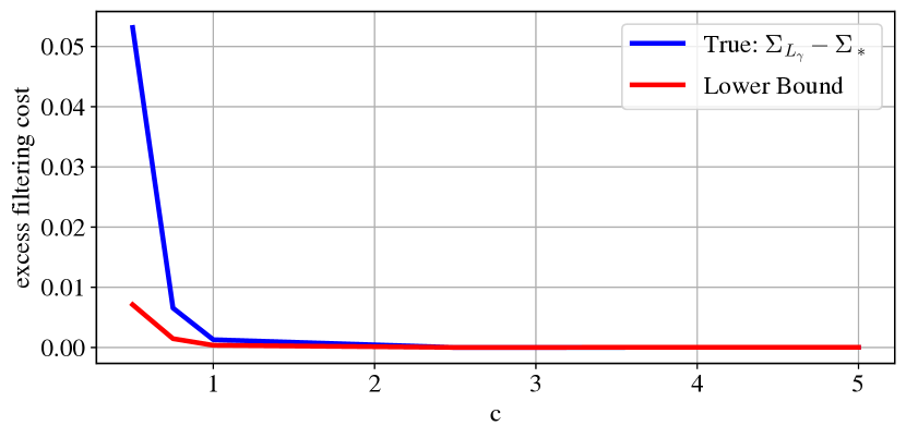
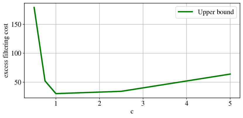
In Figure 1, we demonstrate the upper bound in Theorem 4.3 and the lower bound in Theorem 4.4 for the scalar system with $a=.9$ and varying values of $c$. We fix the robustness level using the soft penalty $\gamma=4$. In both bounds, we substitute the true value of $\xi$, rather than the upper bound. In the upper bound, we also use the value of $Y$ that depends on $\gamma$ rather than the uniform upper bound $\bar{Y}$. We see that the lower bound closely tracks the true cost error. The upper bound follows the same trends as $c$ becomes small, however, it is inflated by several orders of magnitude due to the conservative Riccati perturbation bounds applied. For the upper bound, the lower bound, and the true state prediction error gap, we see that when the observability decreases, as measured by ${\left|c\right|}$ becoming smaller, the gap nominal cost gap between the robust filter and the nominal filter grows.

(a) Lower Bound and True gap

(b) Upper Bound

Figure 1: Upper bound, lower bound, and true excess filtering cost between the robust filter designed with $\gamma=4$ and the nominal filter for a scalar system with $a=0.9$ and and varying values of $c$. As ${\left|c\right|}$ decreases, observability becomes poor. This fact is captured in our bounds, and reflects what occurs with the true excess filtering cost.

(a) Tradeoff Curves

(b) Tradeoff Envelopes

Figure 2: We illustrate the impact of controllability and observability on the severity of the performance robustness tradeoff for state feedback control, state prediction, and output feedback control of the simple integrator system in (34). In Figure 2(a), we plot the tradeoff curves for fixed values of the parameter $\rho$, which determines the controllability and/or observability of the system. The adversarial costs in this setting use $\varepsilon=0.1$, and the tradeoff curves evaluate adversarially robust controllers/observers designed with $\varepsilon\in[0,0.1]$. In Figure 2(b), the envelopes of the tradeoff curves are plotted by evaluating the nominal and $\varepsilon=0.1$-adversarially robust controllers/observers for $\rho\in[0.15,1.0]$. The arrows are in the direction of increasing $\rho$.

Compounding Impact of Poor Controllability and Observability

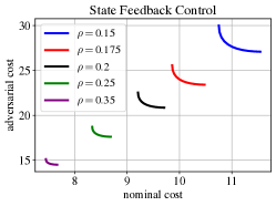
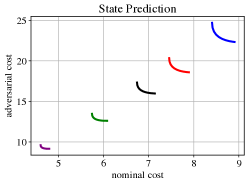
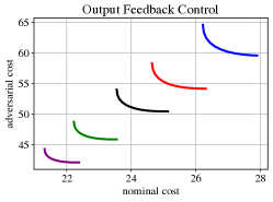
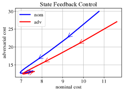
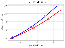
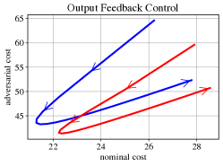
We study the dependence of the tradeoff severity on system controllability and observability in Figure 2. In this example, we consider the two dimensional integrator system defined by

$$x_{t+1} =\begin{bmatrix}1&\rho\\ 0&1\end{bmatrix}x_{t}+\delta_{t}^{x}+w_{t}^{x}+\begin{bmatrix}0\\ 1\end{bmatrix}u_{t},$$ (34)

$$y_{t} =Cx_{t}+\delta_{t}^{y}+w_{t}^{t}.$$ (35)

We consider three settings with this system: state feedback control, state prediction, and output feedback control. In all three settings, $\delta_{t}^{x}$ is an energy budget constrained adversarial input to the state, and $w_{t}^{x}$ is independent zero mean Gaussian noise with identity covariance. For state feedback control, we have $C=I$, $\delta_{t}^{y}=0$ and $w_{t}^{y}=0$. For both state prediction and output feedback control, we take $C=\begin{bmatrix}1&0\end{bmatrix}$, with $\delta_{t}^{y}$ as an adversarial input to the measurement, and $w_{t}^{y}$ as independent zero mean Gaussian noise with covariance 1. For both the control settings (state feedback and output feedback), we set $Q=I$ and $R=1$, and the objective is to minimize the LQR cost. In state prediction, the objective is to minimize the state estimation error with $u_{t}=0$, as described in Section 4. For the state feedback control problem, we study whether poor controllability increases the severity of the performance robustness tradeoffs, as predicted in Section 3. The controllability of the provided system may be varied through the parameter $\rho$: when $\rho$ is small, the system has poor controllability, and as $\rho$ increases, controllability increases. For the state prediction problem, we determine whether poor observability increases the severity of the tradeoff, as predicted in Section 4. The observability of the system may also be varied through the parameter $\rho$: when $\rho$ is small, the observability is poor, and when $\rho$ increases, observability improves. For the output feedback control setting, we study how the impacts of poor observability and controllability compound to result in a severe performance-robustness tradeoff. In Figure 2(a), we consider the tradeoff curves traced out by fixing $\rho$ and then evaluating the nominal and adversarial ($\varepsilon=0.1$) costs of adversarially robust controllers/observers designed with budget $\varepsilon$ varying between $[0,0.1]$. We observe that as controllability and observability decrease, the tradeoff curves shift upward and also widen. This corroborates the trends described in Theorem 3.1 and Theorem 4.1, where we show the bound on the nominal cost gap between adversarially robust and nominal controllers/observers (i.e. width of the tradeoff curve) grows larger as controllability and obserbability decrease, respectively. These trends are further illustrated in Figure 2(b), where we plot the nominal and adversarial ($\varepsilon=0.1$) costs attained by the nominal and adversarially robust ($\varepsilon=0.1$) controllers/observers as a function of $\rho\in[0.15,1]$. We observe that for small $\rho$, the system has poor controllability and observability, hence the distance between the nominal and adversarial costs is large. As controllability and observability increase, this gap decreases monotonically. Note that the costs do not monotonically improve as $\rho$ increases after some point for the control problems, as the amplification of disturbances from the integrator eventually outstrips the benefits of better controllability or observability.

(a) Cartpole setup

(b) Tradeoff Curves

Figure 3: We study the performance-robustness tradeoffs in visual feedback pole-balancing for various fixation points. As the fixation point decreases ($\ell_{0}$ becomes smaller), the observability of the system decreases. The adversarial cost is evaluated with $\varepsilon=0.125$, and the tradeoffs are generated by synthesizing adversarially robust controllers for $\varepsilon\in[0,0.125]$. We see as the fixation point decreases, the tradeoffs for the linearized system become more severe.

Tradeoffs of Linearized Pole Balancing

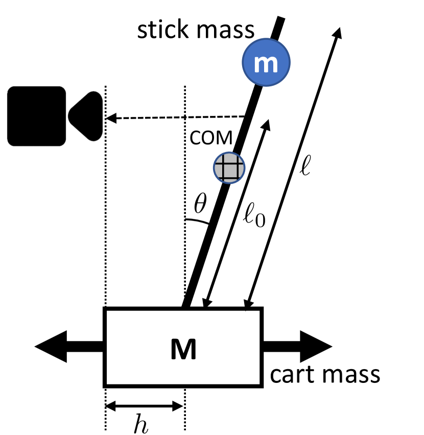
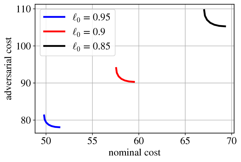
To further illustrate the impact of observability upon the severity of the performance-robustness tradeoff, we consider the example of pole-balancing using visual feedback from a single fixation point on the pole, illustrated in Figure 3. The dynamics of a pole mounted on a cart may be represented as

$$u+w+\delta =(M+m)(\ddot{h}+d_{h}\dot{h})+m\ell((\ddot{\theta}+d_{\theta}\dot{\theta})\cos\theta-\dot{\theta}^{2}\sin\theta),$$ (36)

$$0 =m((\ddot{h}+d_{h}\dot{h})\cos\theta+\ell(\ddot{\theta}+d_{\theta}\dot{\theta})-g\sin\theta),$$

$$y =h+\ell_{0}\sin\theta.$$

This model was proposed in Leong and Doyle (2016) to illustrate the fundamental limitations of control. It was also studied in Xu et al. (2021) to determine how these limitations interact with the sample complexity of learning controllers from data. As depicted in Figure 3(a), $M$ is the mass of the cart, $h$ is the position of the cart, $\theta$ is the angle of the pole, $\ell$ is the length of the pole, and $\ell_{0}$ is the fixation point which the camera observes. The mass of the pole is denoted by $m$ and the acceleration due to gravity by $g$. The damping coefficients are $d_{h}$ and $d_{\theta}$. Our measurement $y$ the distance from the camera to the fixation point. The actuation noise is denoted $w$ and the adversarial input is denoted $\delta$. We consider an instance of this system with $(M,m,\ell,g,d_{h},d_{\theta})=(1,0.1,1,-10,0.2,0.2)$, and various fixation points $\ell_{0}<\ell$. We discretize the dynamics in (36) using Euler discretization with stepsize $0.04$, and linearize the system about the upright equilibrium point. The stochastic noise $w$ is i.i.d. $\mathcal{N}(0,1)$, and the adversarial input $\delta$ is chosen to maximize the cost while falling within the budget $\left\|\delta\right\|^{2}\leq\varepsilon$ on average, where $\varepsilon$ varies as discussed in Figure 3. The cost is specified by $Q=I$, $R=1$. Varying the fixation point varies the observability of the system. In particular, as $l_{0}$ decreases, the observability becomes poor. We plot the tradeoff curves for this system as $l_{0}$ varies in Figure 3(b). As in the integrator experiments, the tradeoff becomes more severe as observability decreases.

Figure 4: Simulations of pole-balancing on the nonlinear continuous time system using linear discrete time controllers. The “nom” controller is the LQG, while the “adv” controller is the adversarially robust controller synthesized with $\varepsilon=0.015$. A mixed $\mathcal{H}_{2}/\mathcal{H}_{\infty}$ baseline is also included. For three different fixation points $\ell_{0}$, the adversarially robust controller outperforms the nominal controller, and similarly to the mixed $\mathcal{H}_{2}/\mathcal{H}_{\infty}$ controller.

Performance of Adversarially Robust Control for Pole Balancing

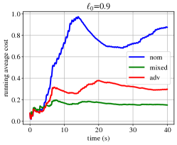
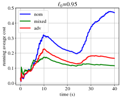
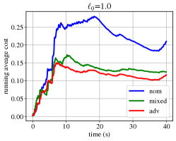
We now use the cartpole system described in the previous example in order to test the performance of the adversarially robust controller in Figure 4. In particular, we simulate the nonlinear continuous time system in (36) under discrete time linear controllers synthesized using the discretized and linearized version of the dynamics. The system parameters and cost matrices are the same as in the previous example, however $\delta$ is modified to enter all states and measurements of the system through an identity mapping to better enhance robustness to the linearization error. We plot the running average cost on the $y$-axis, and the time in seconds on the $x$-axis. In the simulations, the only perturbations impacting the system are zero mean stochastic noise with standard deviation $0.002$ entering the input. The simulations are run for three different fixation points, $\ell_{0}=0.85,0.9$ and $0.95$. For all fixation points we see that the adversarially robust controller performs significantly better than the nominal LQG controller. It is also worth noting that as the fixation point decreases, the total cost increases, and the gap between the two controllers also increases. In particular, as observabilitiy becomes poor, choosing the appropriate level of robustness becomes more essential. A mixed $\mathcal{H}_{2}/\mathcal{H}_{\infty}$ controller is included as an additional baseline. The mixed controller is synthesized in continuous time using the matlab function h2hinfsyn to minimize the $\mathcal{H}_{2}$ norm of the map subject to a constraint that the $\mathcal{H}_{\infty}$ norm is at most 20. We see that the performance of the adversarially robust controller is similar to the mixed $\mathcal{H}_{2}/\mathcal{H}_{\infty}$ controller in all settings. We emphasize that our intent is not to propose a controller which uniformly outperforms mixed $\mathcal{H}_{2}/\mathcal{H}_{\infty}$ controllers, but rather to propose a controller for which we can effectively certify robustness while providing quantitative performance-robustness tradeoffs. The purpose of this experiment is to highlight that the synthesis procedure is effective at producing a controller that enhances general robustness, and achieves performance comparable to existing robust synthesis approaches.

6 Conclusion

We proposed an adversarially robust LQ control problem, and provided sufficient conditions for the optimal solution to this problem, along with an algorithm that converges to the optimal solution when these conditions are satisfied. The solution is closely related to a central suboptimal $\mathcal{H}_{\infty}$ controller. An interesting aspect of this solution is that unlike pure $\mathcal{H}_{2}$ controllers, the adversarially robust controller depends upon the noise statistics. Experiments show that the adversarially robust controller performs similarly to mixed $\mathcal{H}_{2}/\mathcal{H}_{\infty}$ controllers on a simple linear system, and can beat out the LQG in the face of model error arising from linearization.

We used the adversarially robust control problem as a means to study performance-robustness tradeoffs in control. In particular, we derived quantitative upper and lower bounds on the performance gap between the nominal state feedback controller and the adversarially robust state feedback controller. The bounds show that systems with uniformly good controllability have small performance-robustness tradeoffs, while closed-loop nominal systems with a highly controllable mode in the disturbance channel will have a large performance-robustness tradeoff. We also derived bounds on the nominal state estimation error gap of the adversarially robust state estimator compared to the Kalman Filter. In this case, it was shown that systems with uniformly good observability have small tradeoffs. These trends are corroborated by experiments on a simple linear system by tracing out tradeoff curves. One direction for future work is to consider how other adversarial training techniques can be translated to robust controller synthesis and analysis.

Appendix A Proofs from Section 2: Controller Synthesis

A.1 Proof of Lemma 2.1: Soft-constrained State Feedback Solution

Proof: First define the cost to go for a horizon $T$ at step $\tau$.

$$V_{\tau,T}(x_{\tau}):=\min_{u_{\tau:T-1}}\mathbb{E}_{w_{\tau:T-1}}\mathopen{}\left[\max_{\begin{subarray}{c}\delta_{\tau:T-1}\\ causal\end{subarray}}x_{T}^{\top}Qx_{T}+\sum_{t=\tau}^{T-1}x_{t}Qx_{t}+u_{t}^{\top}Ru_{t}-\gamma^{2}\delta_{t}^{\top}\delta_{t}\right]\mathclose{}.$$

Note that for any $T$, $V_{T,T}(x)=x^{\top}Qx$. We will show inductively that $V_{t,T}(x)=x^{\top}P_{t,T}x+q_{t,T}$ for any $t$. To do so, begin with the inductive hypothesis $V_{t+1,T}(x)=x^{\top}P_{t+1,T}x+q_{t+1}$. Applying this hypothesis, we have

$$V_{\tau,T}(x_{\tau}) =x_{\tau}^{\top}Qx_{\tau}+\min_{u_{\tau}}\mathopen{}\left\{u_{\tau}^{\top}Ru_{\tau}+\min_{u_{\tau+1:T-1}}\mathbb{E}_{w_{\tau:T-1}}\mathopen{}\left[\max_{\begin{subarray}{c}\delta_{\tau:T-1}\\ causal\end{subarray}}x_{T}^{\top}Qx_{T}-\delta_{\tau}^{\top}\delta_{\tau}+\sum_{t=\tau+1}^{T-1}x_{t}Qx_{t}+u_{t}^{\top}Ru_{t}-\gamma^{2}\delta_{t}^{\top}\delta_{t}\right]\mathclose{}\right\}\mathclose{}$$

$$=x_{\tau}^{\top}Qx_{\tau}+\min_{u_{\tau}}\bigg{\{}u_{\tau}^{\top}Ru_{\tau}$$

$$+\min_{u_{\tau+1:T-1}}\mathbb{E}_{w_{\tau}}\mathopen{}\left[\max_{\delta_{\tau}}-\gamma^{2}\delta_{\tau}^{\top}\delta_{\tau}+\mathbb{E}_{w_{\tau+1:T-1}}\mathopen{}\left[\max_{\begin{subarray}{c}\delta_{\tau+1:T-1}\\ causal\end{subarray}}x_{T}^{\top}Qx_{T}+\sum_{t=\tau+1}^{T-1}x_{t}Qx_{t}+u_{t}^{\top}Ru_{t}-\gamma^{2}\delta_{t}^{\top}\delta_{t}\right]\mathclose{}\right]\mathclose{}\bigg{\}}$$

$$=x_{\tau}^{\top}Qx_{\tau}+\min_{u_{\tau}}\mathopen{}\left\{u_{\tau}^{\top}Ru_{\tau}+\min_{u_{\tau+1:T-1}}\mathbb{E}_{w_{\tau}}\mathopen{}\left[\max_{\delta_{\tau}}-\gamma^{2}\delta_{\tau}^{\top}\delta_{\tau}+V_{\tau+1,T}(Ax_{\tau}+B_{0}w_{\tau}+B_{1}\delta_{\tau}+B_{2}u_{\tau})\right]\mathclose{}\right\}\mathclose{}$$

$$=x_{\tau}^{\top}Qx_{\tau}+\min_{u_{\tau}}\bigg{\{}u_{\tau}^{\top}Ru_{\tau}$$

$$+\mathbb{E}_{w_{\tau}}\mathopen{}\left[\max_{\delta_{\tau}}-\gamma^{2}\delta_{\tau}^{\top}\delta_{\tau}+(Ax_{\tau}+B_{0}w_{\tau}+B_{1}\delta_{\tau}+B_{2}u_{\tau})^{\top}P_{\tau+1,T}(Ax_{\tau}+B_{0}w_{\tau}+B_{1}\delta_{\tau}+B_{2}u_{\tau})+q_{\tau+1,T}\right]\mathclose{}\bigg{\}}$$

Letting $\phi_{t}:=(Ax_{\tau}+B_{0}w_{\tau}+B_{2}u_{\tau})$, we see that the maximization with respect to $\delta_{\tau}$ is equivalent to

$$\max_{\delta_{\tau}}\delta_{\tau}^{\top}\mathopen{}\left(B_{1}^{\top}P_{\tau+1,T}B_{1}-\gamma^{2}I\right)\mathclose{}\delta_{\tau}^{\top}+2\phi_{\tau}^{\top}P_{\tau+1,T}B_{1}\delta_{\tau}.$$

If $B_{1}^{\top}P_{\tau+1,T}B_{1}\prec\gamma^{2}I$, then there is a unique optimal solution given by $\delta_{\tau}=-(B_{1}^{\top}P_{\tau+1,T}B_{1}-\gamma^{2}I)^{-1}B_{1}^{\top}P_{\tau+1,T}\phi_{\tau}$. Substituting this back in, we see that

$$V_{\tau,T}(x_{\tau}) =q_{\tau+1,T}+x_{\tau}^{\top}Qx_{\tau}+\min_{u_{\tau}}\bigg{\{}u_{\tau}^{\top}Ru_{\tau}+\mathbb{E}_{w_{\tau}}\bigg{[}\phi_{\tau}^{\top}(-\gamma^{2}P_{\tau+1,T}B_{1}(B_{1}^{\top}P_{\tau+1,T}B_{1}-\gamma^{2}I)^{-2}B_{1}^{\top}P_{\tau+1,T}$$

$$\quad\quad+(I-P_{\tau+1,T}B_{1}(B_{1}^{\top}P_{\tau+1,T}B_{1}-\gamma^{2}I)^{-1}B_{1}^{\top})P_{\tau+1,T}(I-B_{1}(B_{1}^{\top}P_{\tau+1,T}B_{1}-\gamma^{2}I)^{-1}B_{1}P_{\tau+1,T}))\phi_{\tau}\bigg{]}\bigg{\}}$$

$$=q_{\tau+1,T}+x_{\tau}^{\top}Qx_{\tau}+\min_{u_{\tau}}\bigg{\{}u_{\tau}^{\top}Ru_{\tau}+\mathbb{E}_{w_{\tau}}\bigg{[}\phi_{\tau}^{\top}(P_{\tau+1,T}+P_{\tau+1,T}B_{1}(\gamma^{2}I-B_{1}^{\top}P_{\tau+1,T}B_{1})^{-1}B_{1}^{\top}P_{\tau+1})\phi_{\tau}\bigg{]}\bigg{\}}.$$

Defining $M_{\tau+1,T}:=P_{\tau+1,T}+P_{\tau+1,T}B_{1}(\gamma^{2}I-B_{1}^{\top}P_{\tau+1,T}B_{1})^{-1}B_{1}^{\top}P_{\tau+1}$, the above expression reduces to

$$q_{\tau+1,T} +x_{\tau}^{\top}Qx_{\tau}+\min_{u_{\tau}}\bigg{\{}u_{\tau}^{\top}Ru_{\tau}+\mathbb{E}_{w_{\tau}}\bigg{[}\phi_{\tau}^{\top}M_{\tau+1}\phi_{\tau}\bigg{]}\bigg{\}}$$

$$=q_{\tau+1,T}+x_{\tau}^{\top}Qx_{\tau}+\min_{u_{\tau}}\bigg{\{}u_{\tau}^{\top}Ru_{\tau}+(Ax_{t}+B_{2}u_{t})^{\top}M_{\tau+1,T}(Ax_{t}+B_{2}u_{t})\bigg{\}}+\operatorname{Tr}(M_{\tau+1,T}B_{0}B_{0}^{\top})$$

Minimizing with respect to $u_{\tau}$ provides

$$u_{\tau}=-(R+B_{2}^{\top}M_{\tau+1,T}B_{2})^{-1}B_{2}^{\top}M_{\tau+1,T}Ax_{\tau}.$$

Substituting this back in, we have

$$V_{\tau,T}(x_{\tau}) =q_{\tau+1,T}+\operatorname{Tr}(M_{\tau+1,T}B_{0}B_{0}^{\top})+x_{\tau}^{\top}\mathopen{}\left(Q+A^{\top}M_{\tau+1,T}A-A^{\top}M_{\tau+1,T}B_{2}(R+B_{2}^{\top}M_{\tau+1,T}B_{2})^{-1}B_{2}^{\top}M_{\tau+1,T}A\right)\mathclose{}x_{\tau}$$

$$=:q_{\tau,T}+x_{\tau}^{\top}P_{\tau,T}x_{\tau}$$

Thus the cost to go is given as

$$V_{\tau,T}(x_{\tau}) =q_{\tau,T}+x_{\tau}^{\top}P_{\tau,T}x_{\tau},$$

where

$$P_{\tau,T} =Q+A^{\top}M_{\tau+1,T}A-A^{\top}M_{\tau+1,T}B_{2}(R+B_{2}^{\top}M_{\tau+1,T}B_{2})^{-1}B_{2}^{\top}M_{\tau+1,T}A$$

$$M_{\tau,T} =P_{\tau,T}+P_{\tau,T}B_{1}\mathopen{}\left(\gamma^{2}I-B_{1}^{\top}P_{\tau,T}B_{1}\right)\mathclose{}^{-1}B_{1}^{\top}P_{\tau,T}$$

$$q_{\tau,T} =q_{\tau+1,T+1}+\operatorname{Tr}(M_{\tau+1,T}B_{0}B_{0}^{\top})$$

$$q_{T,T} =0$$

$$P_{T,T} =Q.$$

Taking the limit as $T\to\infty$, and denoting $P_{\tau}:=P_{\tau,\infty}$ observe that if the iteration

$$P_{\tau} =Q+A^{\top}M_{\tau+1}A-A^{\top}M_{\tau+1}B_{2}(R+B_{2}^{\top}M_{\tau+1}B_{2})^{-1}B_{2}^{\top}M_{\tau+1}A$$

$$M_{\tau} =P_{\tau}+P_{\tau}B_{1}\mathopen{}\left(\gamma^{2}I-B_{1}^{\top}P_{\tau}B_{1}\right)\mathclose{}^{-1}B_{1}^{\top}P_{\tau}$$

converges to a fixed point $P$, then the fixed point must satisfy

$$P_{\gamma} =Q+A^{\top}M_{\gamma}A-A^{\top}M_{\gamma}B_{2}(R+B_{2}^{\top}M_{\gamma}B_{2})^{-1}B_{2}^{\top}M_{\gamma}A$$

$$M_{\gamma} =P_{\gamma}+P_{\gamma}B_{1}\mathopen{}\left(\gamma^{2}I-B_{1}^{\top}P_{\gamma}B_{1}\right)\mathclose{}^{-1}B_{1}P_{\gamma}.$$

Finding a pair $(P_{\gamma},M_{\gamma})$ that satisfy the above conditions is equivalent to finding a $P_{\gamma}$ such that

$$P_{\gamma}=Q+A^{\top}P_{\gamma}A-A^{\top}P_{\gamma}\begin{bmatrix}B_{1}&B_{2}\end{bmatrix}\mathopen{}\left(\begin{bmatrix}B_{1}&B_{2}\end{bmatrix}^{\top}P_{\gamma}\begin{bmatrix}B_{1}&B_{2}\end{bmatrix}+\begin{bmatrix}-\gamma^{2}I&\\ &R\end{bmatrix}\right)\mathclose{}^{-1}\begin{bmatrix}B_{1}&B_{2}\end{bmatrix}^{\top}P_{\gamma}A.$$ (37)

To see that this is the case, note that

$$P_{\gamma}-P_{\gamma}\begin{bmatrix}B_{1}&B_{2}\end{bmatrix}\begin{bmatrix}B_{1}^{\top}P_{\gamma}B_{1}-\gamma^{2}I&B_{1}^{\top}P_{\gamma}B_{2}\\ B_{2}^{\top}P_{\gamma}B_{1}&B_{2}^{\top}P_{\gamma}B_{2}+R\end{bmatrix}^{-1}\begin{bmatrix}B_{1}&B_{2}\end{bmatrix}^{\top}P_{\gamma}$$

$$=P_{\gamma}-P_{\gamma}\begin{bmatrix}B_{1}^{\top}\\ B_{2}^{\top}\end{bmatrix}^{\top}\begin{bmatrix}\Phi_{1}^{-1}+\Phi_{1}^{-1}B_{1}^{\top}P_{\gamma}B_{2}\Phi_{2}^{-1}B_{2}^{\top}P_{\gamma}B_{1}\Phi_{1}^{-1}&\Phi_{1}^{-1}B_{1}^{\top}P_{\gamma}B_{2}\Phi_{2}^{-1}\\ \Phi_{2}^{-1}B_{2}^{\top}P_{\gamma}B_{1}\Phi_{1}^{-1}&\Phi_{2}^{-1}\end{bmatrix}\begin{bmatrix}B_{1}^{\top}\\ B_{2}^{\top}\end{bmatrix}P_{\gamma}$$

$$=M_{\gamma}-M_{\gamma}B_{2}(B_{2}^{\top}M_{\gamma}B_{2}^{\top}+R)^{-1}B_{2}^{\top}M_{\gamma}$$

where $\Phi_{1}=\gamma^{2}I-B_{1}^{\top}PB_{1}$ and $\Phi_{2}=B_{2}^{\top}MB_{2}+R$. The first equality above follows from the inversion formula for a block $2\times 2$ matrix.

By our assumption that there exists a positive semidefinite solution to (11), the iterations converge to this matrix. This can be seen by verifying the monotonicty of the sequence $P_{\tau}$, as in Lemma 3.3 of Basar (1991).

We thus have that in the limit, the cost converges to $\operatorname{Tr}(M_{\gamma}B_{0}B_{0}^{\top})$, where $M_{\gamma}=P_{\gamma}+P_{\gamma}B_{1}(\gamma^{2}I-B_{1}^{\top}P_{\gamma}B_{1})^{-1}B_{1}^{\top}P_{\gamma}$ and $P_{\gamma}$ solves

$$P_{\gamma}=Q+A^{\top}P_{\gamma}A-A^{\top}P_{\gamma}\begin{bmatrix}B_{1}&B_{2}\end{bmatrix}\mathopen{}\left(\begin{bmatrix}B_{1}&B_{2}\end{bmatrix}^{\top}P_{\gamma}\begin{bmatrix}B_{1}&B_{2}\end{bmatrix}+\begin{bmatrix}-\gamma^{2}I&\\ &R\end{bmatrix}\right)\mathclose{}^{-1}\begin{bmatrix}B_{1}&B_{2}\end{bmatrix}^{\top}P_{\gamma}A.$$

Thus a steady state adversarially robust LQR controller at level $\gamma$ is given by

$$u_{t} =F_{\gamma}x_{t}$$

$$F_{\gamma} =-(R+B_{2}^{\top}MB_{2})^{-1}B_{2}^{\top}MA$$

$$M_{\gamma} =P_{\gamma}+P_{\gamma}B_{1}(\gamma^{2}I-B_{1}^{\top}P_{\gamma}B_{1})^{-1}B_{1}^{\top}P_{\gamma}$$

$$P_{\gamma} \mbox{ solves \eqref{eq:modified DARE}},$$

and the optimal adversarial perturbation is given by

$$\delta_{t}=(\gamma^{2}I-B_{1}^{\top}P_{\gamma}B_{1})^{-1}B_{1}^{\top}P_{\gamma}((A+BKx_{t})+B_{0}w_{t}).$$

This may be expressed compactly as

$$\begin{bmatrix}\delta_{t}\\ u_{t}\end{bmatrix} =\begin{bmatrix}E_{\gamma}\\ F_{\gamma}\end{bmatrix}x_{t}+\begin{bmatrix}\Delta_{\gamma}\\ 0\end{bmatrix}w_{t}$$

$$\begin{bmatrix}E_{\gamma}\\ F_{\gamma}\end{bmatrix} =-\mathopen{}\left(\begin{bmatrix}B_{1}&B_{2}\end{bmatrix}^{\top}P_{\gamma}\begin{bmatrix}B_{1}&B_{2}\end{bmatrix}+\begin{bmatrix}-\gamma^{2}I\\ &R\end{bmatrix}\right)\mathclose{}^{-1}\begin{bmatrix}B_{1}&B_{2}\end{bmatrix}^{\top}P_{\gamma}A$$

$$\Delta =(\gamma^{2}I-B_{1}^{\top}P_{\gamma}B_{1})^{-1}B_{1}^{\top}P_{\gamma}B_{0}.$$

To verify that the controller is stabilizing, it suffices to note that the cost is finite. Leveraging the fact that $(Q^{1/2},A)$ is detectable thus tells us that the state must converge to zero in the absence of noise.

For necessity of the given conditions, first note that if there is no PSD solution to the Riccati equation, then the value does not converge. If the condition $B_{1}^{\top}P_{\gamma}B_{1}\prec\gamma^{2}I$ is not satisfied, then the adversarial maximization problem is not strictly concave, and it may supply arbitrarily large perturbations. $\blacksquare$

A.2 Proof of Lemma 2.2: Soft-Constrained Output Feedback Solution

We leverage the approach developed in Doyle et al. (1989a) (see Zhou et al. (1996) for reference), which was extended to Iglesias and Glover (1991) for discrete time systems. In particular, we solve this problem via a combination of the state feedback solution, and the full control solution. To do so, we demonstrate that the optimal solution for output feedback control reduces to estimating the optimal state feedback control action. The resulting problem is known as output estimation, which may be reduced to a full control problem, and solved via dynamic programming.

Definition A.1

The soft constrained adversarially robust output feedback, full control, and output estimation problems all attempt to minimize the objective

$$\limsup_{T\to\infty}\frac{1}{T}\mathbb{E}\mathopen{}\left[\max_{\bm{\delta}\mbox{ causal}}\sum_{t=0}^{T-1}\left\|z_{t}\right\|^{2}-\gamma^{2}\left\|\delta_{t}\right\|^{2}\right]\mathclose{}.$$

The difference lies in the information available to the controller, and the channel that the control enters.

• The adversarially robust output feedback control problem may consider a general plant of the form

  $$\left[\begin{array}[]{c|ccc}A&B_{0}&B_{1}&B_{2}\\ \hline\cr C_{1}&D_{10}&D_{11}&D_{21}\\ C_{2}&D_{20}&D_{21}&0\end{array}\right].$$

• The adverarially robust output estimation problem considers a plant of the form

  $$\left[\begin{array}[]{c|ccc}A&B_{0}&B_{1}&B_{2}\\ \hline\cr C_{1}&D_{10}&D_{11}&I\\ C_{1}&D_{20}&D_{21}&0\end{array}\right].$$

• The adversarially robust full control problem assumes complete actuation of both the state and the performance signal:

  $$\left[\begin{array}[]{c|ccc}A&B_{0}&B_{1}&\begin{bmatrix}I&0\end{bmatrix}\\ \hline\cr C_{1}&D_{10}&D_{11}&\begin{bmatrix}0&I\end{bmatrix}\\ C_{2}&D_{20}&D_{21}&0\end{array}\right].$$

Our first objective will be to reduce the output feedback problem to an output estimation problem. This motivates the following lemma.

Lemma A.1

Suppose that $P_{\gamma}$ solves

$$P_{\gamma} =A^{\top}P_{\gamma}A+Q-A^{\top}P_{\gamma}\begin{bmatrix}B_{1}&B_{2}\end{bmatrix}\mathopen{}\left(\begin{bmatrix}B_{1}&B_{2}\end{bmatrix}^{\top}P_{\gamma}\begin{bmatrix}B_{1}&B_{2}\end{bmatrix}+\begin{bmatrix}-\gamma^{2}I\\ &R\end{bmatrix}\right)\mathclose{}^{-1}\begin{bmatrix}B_{1}&B_{2}\end{bmatrix}P_{\gamma}A,$$ (38)

and that there exists a nonsingular matrix $\begin{bmatrix}\hat{T}_{11}&0\\ \hat{T}_{21}&\hat{T}_{22}\end{bmatrix}$ with $\hat{T}_{11}\in\mathbb{R}^{n_{\delta}\times n_{\delta}}$, and $\hat{T}_{22}\in\mathbb{R}^{n_{u}\times n_{u}}$ such that

$$\Psi:=\begin{bmatrix}B_{1}&B_{2}\end{bmatrix}^{\top}P_{\gamma}\begin{bmatrix}B_{1}&B_{2}\end{bmatrix}+\begin{bmatrix}-\gamma^{2}I\\ &R\end{bmatrix}=\begin{bmatrix}\hat{T}_{11}&0\\ \hat{T}_{21}&\hat{T}_{22}\end{bmatrix}^{\top}\begin{bmatrix}-I\\ &I\end{bmatrix}\begin{bmatrix}\hat{T}_{11}&0\\ \hat{T}_{21}&\hat{T}_{22}\end{bmatrix}.$$ (39)

Then for the closed-loop system under any controller $K$,

$$\limsup_{T}\frac{1}{T}\mathbb{E}_{w}\mathopen{}\left[\sup_{\delta\textrm{causal}}\sum_{t=0}^{T-1}\left\|z_{t}\right\|^{2}-\gamma^{2}\left\|\delta_{t}\right\|^{2}\right]\mathclose{}=\limsup_{T}\frac{1}{T}\mathbb{E}_{w}\mathopen{}\left[\sup_{r\textrm{causal}}\sum_{t=0}^{T-1}\left\|\nu_{t}\right\|^{2}-\gamma^{2}\left\|r_{t}\right\|^{2}+w_{t}^{\top}J_{\gamma}w_{t}\right]\mathclose{},$$

where

$$r_{t} =\hat{T}_{11}(\delta_{t}-E_{\gamma}x_{t}-\Delta_{\gamma}w_{t})$$

$$\nu_{t} =\hat{T}_{21}\delta+\hat{T}_{22}u-\begin{bmatrix}\hat{T}_{21}&\hat{T}_{22}\end{bmatrix}\mathopen{}\left(\begin{bmatrix}E_{\gamma}\\ F_{\gamma}\end{bmatrix}x_{t}+\begin{bmatrix}\Delta_{\gamma}\\ 0\end{bmatrix}w_{t}\right)\mathclose{}$$

$$J_{\gamma} =B_{0}^{\top}P_{\gamma}B_{1}\mathopen{}\left(\gamma^{2}I-B_{1}^{\top}P_{\gamma}B_{1}\right)\mathclose{}^{-1}B_{1}^{\top}P_{\gamma}B_{0}+B_{0}^{\top}P_{\gamma}B_{0},$$

and

$$\begin{bmatrix}E_{\gamma}\\ F_{\gamma}\end{bmatrix} =\Psi^{-1}\begin{bmatrix}B_{1}&B_{2}\end{bmatrix}^{\top}PA,$$ (40)

$$\Delta_{\gamma} =(\gamma^{2}I-B_{1}^{\top}PB_{1})^{-1}B_{1}^{\top}PB_{0}.$$

Proof: For any $u_{t}$, $\delta_{t}$, and $w_{t}$,

$$\mathopen{}\left(\begin{bmatrix}\delta_{t}\\ u_{t}\end{bmatrix}-\begin{bmatrix}E_{\gamma}\\ F_{\gamma}\end{bmatrix}x_{t}-\begin{bmatrix}\Delta_{\gamma}\\ 0\end{bmatrix}w_{t}\right)\mathclose{}^{\top}\Psi\mathopen{}\left(\begin{bmatrix}\delta_{t}\\ u_{t}\end{bmatrix}-\begin{bmatrix}E_{\gamma}\\ F_{\gamma}\end{bmatrix}x_{t}-\begin{bmatrix}\Delta_{\gamma}\\ 0\end{bmatrix}w_{t}\right)\mathclose{}$$

$$=\begin{bmatrix}\delta_{t}\\ u_{t}\end{bmatrix}^{\top}\mathopen{}\left(\begin{bmatrix}0\\ &R\end{bmatrix}+\begin{bmatrix}B_{1}&B_{2}\end{bmatrix}^{\top}P_{\gamma}\begin{bmatrix}B_{1}&B_{2}\end{bmatrix}\right)\mathclose{}\begin{bmatrix}\delta_{t}\\ u_{t}\end{bmatrix}-\gamma^{2}\left\|\delta_{t}\right\|^{2}$$

$$-\mathopen{}\left(\begin{bmatrix}E_{\gamma}\\ F_{\gamma}\end{bmatrix}x_{t}+\begin{bmatrix}\Delta_{\gamma}\\ 0\end{bmatrix}w_{t}\right)\mathclose{}^{\top}\Psi\begin{bmatrix}\delta_{t}\\ u_{t}\end{bmatrix}-\begin{bmatrix}\delta_{t}\\ u_{t}\end{bmatrix}^{\top}\Psi\mathopen{}\left(\begin{bmatrix}E_{\gamma}\\ F_{\gamma}\end{bmatrix}x_{t}+\begin{bmatrix}\Delta_{\gamma}\\ 0\end{bmatrix}w_{t}\right)\mathclose{}+\mathopen{}\left(\begin{bmatrix}E_{\gamma}\\ F_{\gamma}\end{bmatrix}x_{t}+\begin{bmatrix}\Delta_{\gamma}\\ 0\end{bmatrix}w_{t}\right)\mathclose{}^{\top}\Psi\mathopen{}\left(\begin{bmatrix}E_{\gamma}\\ F_{\gamma}\end{bmatrix}x_{t}+\begin{bmatrix}\Delta_{\gamma}\\ 0\end{bmatrix}w_{t}\right)\mathclose{}$$

$$=\left\|z_{t}\right\|^{2}-\gamma^{2}\left\|\delta_{t}\right\|^{2}-x_{t}^{\top}\mathopen{}\left(C_{1}^{\top}C_{1}-\begin{bmatrix}E_{\gamma}\\ F_{\gamma}\end{bmatrix}^{\top}\Psi\begin{bmatrix}E_{\gamma}\\ F_{\gamma}\end{bmatrix}\right)\mathclose{}x_{t}+\begin{bmatrix}\delta_{t}\\ u_{t}\end{bmatrix}^{\top}\begin{bmatrix}B_{1}&B_{2}\end{bmatrix}^{\top}P_{\gamma}\begin{bmatrix}B_{1}&B_{2}\end{bmatrix}\begin{bmatrix}\delta_{t}\\ u_{t}\end{bmatrix}^{\top}$$

$$\qquad+2\mathopen{}\left(\begin{bmatrix}B_{1}&B_{2}\end{bmatrix}^{\top}P_{\gamma}Ax_{t}+\begin{bmatrix}B_{1}&B_{1}(\gamma^{2}I-B_{1}^{\top}P_{\gamma}B_{1})^{-1}B_{1}^{\top}P_{\gamma}B_{2}\end{bmatrix}^{\top}P_{\gamma}B_{0}w_{t}\right)\mathclose{}^{\top}\begin{bmatrix}\delta_{t}\\ u_{t}\end{bmatrix}+2x_{t}^{\top}A^{\top}P_{\gamma}\begin{bmatrix}B_{1}&B_{2}\end{bmatrix}\begin{bmatrix}\Delta_{\gamma}\\ 0\end{bmatrix}w_{t}$$

$$\qquad+w_{t}^{\top}\begin{bmatrix}\Delta_{\gamma}\\ 0\end{bmatrix}^{\top}\Psi\begin{bmatrix}\Delta_{\gamma}\\ 0\end{bmatrix}w_{t}$$

$$=\left\|z_{t}\right\|^{2}-\gamma^{2}\left\|\delta_{t}\right\|^{2}-x_{t}^{\top}P_{\gamma}x_{t}+\mathopen{}\left(Ax_{t}+\begin{bmatrix}B_{1}&B_{2}\end{bmatrix}\begin{bmatrix}\delta_{t}\\ u_{t}\end{bmatrix}\right)\mathclose{}^{\top}P_{\gamma}\mathopen{}\left(Ax_{t}+\begin{bmatrix}B_{1}&B_{2}\end{bmatrix}\begin{bmatrix}\delta_{t}\\ u_{t}\end{bmatrix}\right)\mathclose{}$$

$$\qquad+2\mathopen{}\left(\begin{bmatrix}B_{1}&B_{1}(\gamma^{2}I-B_{1}^{\top}P_{\gamma}B_{1})^{-1}B_{1}^{\top}P_{\gamma}B_{2}\end{bmatrix}^{\top}P_{\gamma}B_{0}w_{t}\right)\mathclose{}^{\top}\begin{bmatrix}\delta_{t}\\ u_{t}\end{bmatrix}+2x_{t}^{\top}A^{\top}P_{\gamma}\begin{bmatrix}B_{1}&B_{2}\end{bmatrix}\begin{bmatrix}\Delta_{\gamma}\\ 0\end{bmatrix}w_{t}+w_{t}^{\top}\begin{bmatrix}\Delta_{\gamma}\\ 0\end{bmatrix}^{\top}\Psi\begin{bmatrix}\Delta_{\gamma}\\ 0\end{bmatrix}w_{t}$$

$$=\left\|z_{t}\right\|^{2}-\gamma^{2}\left\|\delta_{t}\right\|^{2}-x_{t}^{\top}P_{\gamma}x_{t}+\mathopen{}\left(x_{t+1}\right)\mathclose{}^{\top}P_{\gamma}\mathopen{}\left(x_{t+1}\right)\mathclose{}+2u_{t}^{\top}B_{2}^{\top}\mathopen{}\left(P_{\gamma}B_{1}(\gamma^{2}I-B_{1}^{\top}P_{\gamma}B_{1})^{-1}B_{1}^{\top}P_{\gamma}-P_{\gamma}\right)\mathclose{}B_{0}w_{t}$$

$$\qquad+2x_{t}^{\top}A^{\top}(P_{\gamma}B_{1}(\gamma^{2}I-B_{1}^{\top}P_{\gamma}B_{1})^{-1}B_{1}^{\top}P_{\gamma}-P_{\gamma})B_{0}w_{t}-w_{t}^{\top}B_{0}^{\top}\mathopen{}\left(P_{\gamma}B_{1}(\gamma^{2}I-B_{1}^{\top}P_{\gamma}B_{1})^{-1}B_{1}^{\top}P_{\gamma}+P_{\gamma}\right)\mathclose{}B_{0}w_{t},$$

where we have made use of (38) and (40). Summing over time, maximizing over causal $\delta$, taking the expectation with respect to $w$, and taking the limit yields

$$\limsup_{T}\frac{1}{T}\mathbb{E}_{w}\mathopen{}\left[\sup_{\delta\textrm{ causal}}\sum_{t=0}^{T-1}\mathopen{}\left(\begin{bmatrix}\delta_{t}\\ u_{t}\end{bmatrix}-\begin{bmatrix}E_{\gamma}\\ F_{\gamma}\end{bmatrix}x_{t}-\begin{bmatrix}\Delta_{\gamma}\\ 0\end{bmatrix}w_{t}\right)\mathclose{}^{\top}\Psi\mathopen{}\left(\begin{bmatrix}\delta_{t}\\ u_{t}\end{bmatrix}-\begin{bmatrix}E_{\gamma}\\ F_{\gamma}\end{bmatrix}x_{t}-\begin{bmatrix}\Delta_{\gamma}\\ 0\end{bmatrix}w_{t}\right)\mathclose{}\right]\mathclose{}$$

$$=\limsup_{T}\frac{1}{T}\mathbb{E}_{w}\mathopen{}\left[\sup_{\delta\textrm{ causal}}\left\|z\right\|^{2}-\gamma^{2}\left\|\delta\right\|^{2}+w_{t}^{\top}J_{\gamma}w_{t}\right]\mathclose{}$$

where $J_{\gamma}=B_{0}^{\top}\mathopen{}\left(P_{\gamma}B_{1}(\gamma^{2}I-B_{1}^{\top}P_{\gamma}B_{1})^{-1}B_{1}^{\top}P_{\gamma}+P_{\gamma}\right)\mathclose{}B_{0}$. Note that we have used the fact that $w_{t}$ is independent from $x_{t}$ and $u_{t}$ due to causality. Using the decomposition of $\Psi$ in (39), we find

$$\mathopen{}\left(\begin{bmatrix}\delta_{t}\\ u_{t}\end{bmatrix}-\begin{bmatrix}E_{\gamma}\\ F_{\gamma}\end{bmatrix}x_{t}-\begin{bmatrix}\Delta_{\gamma}\\ 0\end{bmatrix}w_{t}\right)\mathclose{}^{\top}\Psi\mathopen{}\left(\begin{bmatrix}\delta_{t}\\ u_{t}\end{bmatrix}-\begin{bmatrix}E_{\gamma}\\ F_{\gamma}\end{bmatrix}x_{t}-\begin{bmatrix}\Delta_{\gamma}\\ 0\end{bmatrix}w_{t}\right)\mathclose{}$$

$$=\left\|\hat{T}_{21}\delta_{t}+\hat{T}_{22}u_{t}-\begin{bmatrix}\hat{T}_{21}&\hat{T}_{22}\end{bmatrix}\mathopen{}\left(\begin{bmatrix}E_{\gamma}\\ F_{\gamma}\end{bmatrix}x_{t}+\begin{bmatrix}\Delta_{\gamma}\\ 0\end{bmatrix}w_{t}\right)\mathclose{}\right\|^{2}-\left\|\hat{T}_{11}(\delta_{t}-E_{\gamma}x_{t}-\Delta_{\gamma}w_{t})\right\|^{2}$$

$$=\left\|\nu_{t}\right\|^{2}-\left\|r_{t}\right\|^{2}.$$

$\blacksquare$

We have thus reduced the adversarially robust partially observed control problem to the adversarially robust partially observed problem for the following system:

$$x_{t+1} =(A+B_{1}E_{\gamma})x_{t}+(B_{0}+B_{1}\Delta_{\gamma})w_{t}+B_{1}\hat{T}_{11}^{-1}r_{t}+B_{2}u_{t}$$

$$\nu_{t} =-\hat{T}_{22}F_{\gamma}x_{t}+\hat{T}_{21}\hat{T}_{11}^{-1}r_{t}+\hat{T}_{22}u_{t}$$

$$y_{t} =(C_{2}+D_{21}E_{\gamma})x_{t}+(D_{20}+D_{21}\Delta_{\gamma})w_{t}+D_{21}\hat{T}_{11}^{-1}r_{t}.$$

As $\hat{T}_{22}$ is invertible, the optimal solution to the above problem is given by $\hat{T}_{22}^{-1}K$, where $K$ solves the output estimation problem

$$\inf_{K}\limsup_{T}\frac{1}{T}\mathbb{E}_{w}\mathopen{}\left[\sup_{r\textrm{ causal}}\sum_{t=0}^{T-1}\left\|\nu_{t}\right\|^{2}-\left\|r_{t}\right\|^{2}\right]\mathclose{}$$

under the system

$$x_{t+1} =(A+B_{1}E_{\gamma})x_{t}+(B_{0}+B_{1}\Delta_{\gamma})w_{t}+B_{1}\hat{T}_{11}^{-1}r_{t}+B_{2}\hat{T}_{22}^{-1}u_{t}$$

$$\nu_{t} =-\hat{T}_{22}F_{\gamma}x_{t}+\hat{T}_{21}\hat{T}_{11}^{-1}r_{t}+u_{t}$$

$$y_{t} =(C_{2}+D_{21}E_{\gamma})x_{t}+(D_{20}+D_{21}\Delta_{\gamma})w_{t}+D_{21}\hat{T}_{11}^{-1}r_{t}.$$

We therefore recall the following change of variables:

$$\left[\begin{array}[]{c|ccc}\hat{A}&\hat{B}_{0}&\hat{B}_{1}&\hat{B}_{2}\\ \hline\cr\hat{C}_{1}&0&\hat{D}_{11}&I\\ \hat{C}_{2}&\hat{D}_{20}&\hat{D}_{21}&0\end{array}\right]=\left[\begin{array}[]{c|ccc}A+B_{1}E_{\gamma}&B_{0}+B_{1}\Delta_{\gamma}&\hat{B}_{1}\hat{T}_{11}^{-1}&B_{2}\hat{T}_{22}^{-1}\\ \hline\cr-\hat{T}_{22}F_{\gamma}&0&\hat{T}_{21}\hat{T}_{11}^{-1}&I\\ C_{2}+D_{21}E_{\gamma}&D_{20}+D_{21}\Delta_{\gamma}&\hat{D}_{21}\hat{T}_{11}^{-1}&0\end{array}\right].$$

Note that by the fact that the controller gain and adversarial pertubation are derived from Lemma 2.1, the matrix $\hat{A}-\hat{B}_{2}\hat{C}_{1}$ is stable. Then the following lemma allows us to reduce the above output estimation problem to a full control problem, i.e. a problem where the input directly enters the state and the performance signal.

Lemma A.2

If $\hat{A}-\hat{B}_{2}\hat{C}_{1}$ is stable, then the adversarially robust output estimation problem defined by the system

$$G_{AOE}=\left[\begin{array}[]{c|ccc}\hat{A}&\hat{B}_{0}&\hat{B}_{1}&\hat{B}_{2}\\ \hline\cr\hat{C}_{1}&0&\hat{D}_{11}&I\\ \hat{C}_{2}&\hat{D}_{20}&\hat{D}_{21}&0\end{array}\right]$$

may be reduced to the adversarially robust full control problem for a system

$$G_{AFC}=\left[\begin{array}[]{c|ccc}\hat{A}&\hat{B}_{0}&\hat{B}_{1}&\begin{bmatrix}I&0\end{bmatrix}\\ \hline\cr\hat{C}_{1}&0&\hat{D}_{11}&\begin{bmatrix}0&I\end{bmatrix}\\ \hat{C}_{2}&\hat{D}_{20}&\hat{D}_{21}&0\end{array}\right].$$

In particular, suppose that $K_{AFC}$ solves the adversarially robust full control problem. Then $K_{AOE}$ defined by $\mathcal{F}_{l}(P_{AOE},K_{AFC})$ with

$$P_{AOE}=\left[\begin{array}[]{c| cc}\hat{A}-\hat{B}_{2}\hat{C}_{1}&0&\begin{bmatrix}I&-B_{2}\end{bmatrix}\\ \hline\cr\hat{C}_{1}&0&\begin{bmatrix}0&I\end{bmatrix}\\ \hat{C}_{2}&I&0\end{array}\right]$$

solves the adversarially robust output estimation problem. Similarly, if $K_{AOE}$ solves the adversarially robust output estimation problem, then $K_{AFC}$ defined by $\begin{bmatrix}\hat{B}_{2}\\ I\end{bmatrix}K_{AOE}$ solves the adversarially robust full control problem.

Proof: The result of Theorem 12.6 of Zhou and Doyle (1998) tells us that if $K_{AOE}$ internally stabilizes $G_{AOE}$, then $K_{AFC}=\begin{bmatrix}\hat{B}_{2}\\ I\end{bmatrix}K_{AOE}$ internally stabilizes $G_{AOE}$, and $\mathcal{F}_{l}(G_{AFC},K_{AFC})=\mathcal{F}_{l}(G_{AOE},K_{AOE})$. Similarly, if $K_{AFC}$ internally stabilizes $G_{AFC}$, then $K_{AOE}=\mathcal{F}_{l}(P_{AOE},K_{AFC})$ internally stabilzes $G_{AFC}$, and $\mathcal{F}_{l}(G_{AFC},K_{AFC})=\mathcal{F}_{l}(G_{AOE},K_{AOE})$. As the transfer functions are equal, a solution to either the adversarially robust output estimation problem or the adversarially robust full control problem provides the solution to the other. $\blacksquare$

Lemma A.3

Consider the adversarially robust full control problem defined by

$$G_{AFC}=\left[\begin{array}[]{c|ccc}\hat{A}&\hat{B}_{0}&\hat{B}_{1}&\begin{bmatrix}I&0\end{bmatrix}\\ \hline\cr\hat{C}_{1}&0&\hat{D}_{11}&\begin{bmatrix}0&I\end{bmatrix}\\ \hat{C}_{2}&\hat{D}_{20}&\hat{D}_{21}&0\end{array}\right].$$

Suppose there exists real matrices $L_{\gamma},N_{\gamma},\Sigma_{\gamma},Y_{\gamma}$ with $\Sigma_{\gamma}$ and $Y_{\gamma}$ symmetric positive definite that satisfy

$$\tilde{A} =\hat{A}+L_{\gamma}\hat{C}_{2}$$ (41)

$$\tilde{B}_{0} =\hat{B}_{0}+L_{\gamma}\hat{D}_{20}$$

$$\tilde{B}_{1} =\hat{B}_{1}+L_{\gamma}\hat{D}_{21}$$

$$\tilde{C}_{1} =\hat{C}_{1}+N_{\gamma}\hat{C}_{2}$$

$$\tilde{D}_{11} =\hat{D}_{11}+N_{\gamma}\hat{D}_{21}$$

$$\tilde{D}_{10} =N_{\gamma}\hat{D}_{20}$$

$$\Phi =I-\tilde{D}_{11}^{\top}\tilde{D}_{11}-\tilde{B}_{1}^{\top}Y_{\gamma}\tilde{B}_{1}\succ 0$$

$$Y_{\gamma} =\tilde{C}_{1}^{\top}\tilde{C}_{1}+\tilde{A}^{\top}Y_{\gamma}\tilde{A}+\mathopen{}\left(\tilde{D}_{11}^{\top}\tilde{C}_{1}+\tilde{B}_{1}^{\top}Y_{\gamma}\tilde{A}\right)\mathclose{}^{\top}\Phi^{-1}\mathopen{}\left(\tilde{D}_{11}^{\top}\tilde{C}_{1}+\tilde{B}_{1}^{\top}Y_{\gamma}\tilde{A}\right)\mathclose{}$$

$$\Sigma_{\gamma} =\mathopen{}\left[(I+\tilde{B}_{1}\Phi^{-1}\tilde{B}_{1}^{\top}Y_{\gamma})\tilde{A}+\tilde{B}_{1}\Phi^{-1}\tilde{D}_{11}^{\top}\tilde{C}_{1}\right]\mathclose{}\Sigma_{\gamma}\mathopen{}\left[(I+\tilde{B}_{1}\Phi^{-1}\tilde{B}_{1}^{\top}Y_{\gamma})\tilde{A}+\tilde{B}_{1}\Phi^{-1}\tilde{D}_{11}^{\top}\tilde{C}_{1}\right]\mathclose{}^{\top}$$

$$\qquad+\mathopen{}\left[(I+\tilde{B}_{1}\Phi^{-1}\tilde{B}_{1}^{\top}Y_{\gamma})\tilde{B}_{0}+\tilde{B}_{1}^{\top}\Phi^{-1}\tilde{D}_{11}^{\top}\tilde{D}_{10}\right]\mathclose{}\mathopen{}\left[(I+\tilde{B}_{1}\Phi^{-1}\tilde{B}_{1}^{\top}Y_{\gamma})\tilde{B}_{0}+\tilde{B}_{1}^{\top}\Phi^{-1}\tilde{D}_{11}^{\top}\tilde{D}_{10}\right]\mathclose{}^{\top}$$

$$L_{\gamma},N_{\gamma} \in\operatorname*{argmin}_{L,N}\operatorname{Tr}\mathopen{}\left(\tilde{D}_{10}^{\top}\tilde{D}_{10}+\tilde{B}_{0}^{\top}Y_{\gamma}\tilde{B}_{0}+(\tilde{D}_{10}^{\top}\tilde{D}_{11}+\tilde{B}_{0}^{\top}Y_{\gamma}\tilde{B}_{1})\Phi^{-1}(\tilde{D}_{10}^{\top}\tilde{D}_{11}+\tilde{B}_{0}^{\top}Y_{\gamma}\tilde{B}_{1})^{\top}\right)\mathclose{}$$

$$\qquad\qquad+\operatorname{Tr}\mathopen{}\left(\Sigma_{\gamma}\mathopen{}\left[\tilde{C}_{1}^{\top}\tilde{C}_{1}+\tilde{A}^{\top}Y_{\gamma}\tilde{A}+(\tilde{D}_{11}^{\top}\tilde{C}_{1}+\tilde{B}_{1}^{\top}Y_{\gamma}\tilde{A})^{\top}\Phi^{-1}(\tilde{D}_{11}^{\top}\tilde{C}_{1}+\tilde{B}_{1}^{\top}Y_{\gamma}\tilde{A})\right]\mathclose{}\right)\mathclose{},$$

where $Y_{\gamma}$ and $\Sigma_{\gamma}$ are treated as fixed parameters in the minimization problem in the final lines. Then an optimal solution to the adversarially robust full control problem is given by the static controller with gain $\begin{bmatrix}L_{\gamma}\\ N_{\gamma}\end{bmatrix}$.

Proof: We will first solve the finite horizon version of the problem under the assumption that the optimal controller consists of time varying static gains of the form $\begin{bmatrix}L_{t}\\ N_{t}\end{bmatrix}$. The finite horizon $\gamma$-adversarially robust full control problem under this assumption may be written as

$$J_{\star}=\operatorname*{minimize}_{L_{0},N_{0},\dots,L_{T-1},N_{T-1}}\mathbb{E}_{x_{0},w_{0:T-1}}\mathopen{}\left[\sup_{r\textrm{ causal}}\sum_{t=0}^{T-1}\left\|\hat{C}_{1}x_{t}+\hat{D}_{11}r_{t}+N_{t}y_{t}\right\|^{2}-\left\|r_{t}\right\|^{2}\right]\mathclose{}$$

where $x_{0}\sim\mathcal{N}(0,\Sigma_{0})$, and $x_{t}$ progresses according to dynamics

$$x_{t+1}=(\hat{A}+L_{t}\hat{C}_{2})x_{t}+(\hat{B}_{0}+L_{t}\hat{D}_{20})w_{t}+(\hat{B}_{1}+L_{t}\hat{D}_{11})r_{t}.$$

We will see that under the optimal adversarial pertubation and filter gain, the state is distributed as $x_{t}\sim\mathcal{N}(0,\Sigma_{t})$ for $t=0,\dots,T$. We will define the cost to go in terms of the variance of the state. In particular, define

$$V_{\tau}(\Sigma_{\tau})=\operatorname*{minimize}_{L_{\tau},N_{\tau}\dots,L_{T-1},N_{T-1}}\mathbb{E}_{x_{\tau},w_{\tau:T-1}}\mathopen{}\left[\sup_{r\textrm{ causal}}\sum_{t=\tau}^{T-1}\left\|\hat{C}_{1}x_{t}+\hat{D}_{11}r_{t}+N_{t}y_{t}\right\|^{2}-\left\|r_{t}\right\|^{2}\right]\mathclose{}$$

so that $J_{\star}=V_{0}(\Sigma_{0})$. To derive the optimal gains $L_{t}$ and $N_{t}$, we will show that there exists some $Y_{\tau}\succeq 0$ such that $V_{\tau}(\Sigma_{\tau})=\operatorname{Tr}(\Sigma_{\tau}Y_{\tau})+q_{\tau}$ for all $\tau$. The base case is clear $V_{T}(\Sigma_{T})=\operatorname{Tr}(\Sigma_{T}Y_{T})$ where $Y_{T}=0$. Assume that this is true at time $\tau+1$, i.e. assume that $V_{\tau+1}=\operatorname{Tr}(\Sigma_{\tau+1}Y_{\tau+1})+q_{\tau+1}$. Then we have that

$$V_{\tau}(\Sigma_{\tau}) =\operatorname*{minimize}_{L_{\tau},N_{\tau},\dots,L_{T-1},N_{T-1}}\mathbb{E}_{x_{\tau},w_{\tau:T-1}}\mathopen{}\left[\max_{r_{\tau:T-1}\textrm{causal}}\sum_{t=\tau}^{T-1}\left\|\hat{C}_{1}x_{t}+\hat{D}_{11}r_{t}+N_{t}y_{t}\right\|^{2}-\left\|r_{t}\right\|^{2}\right]\mathclose{}$$

$$=\operatorname*{minimize}_{L_{\tau},N_{\tau}}\mathbb{E}_{x_{\tau},w_{\tau}}\mathopen{}\left[\sup_{r_{\tau}}\left\|\hat{C}_{1}x_{\tau}+\hat{D}_{11}r_{\tau}+N_{\tau}y_{\tau}\right\|^{2}-\left\|r_{\tau}\right\|^{2}+V_{\tau+1}(\Sigma_{\tau+1})\right]\mathclose{}$$

$$=\operatorname*{minimize}_{L_{\tau},N_{\tau}}\mathbb{E}_{x_{\tau},w_{\tau}}\mathopen{}\left[\sup_{r_{\tau}}\left\|\hat{C}_{1}x_{\tau}+\hat{D}_{11}r_{\tau}+N_{t}y_{t}\right\|^{2}-\left\|r_{\tau}\right\|^{2}+x_{\tau+1}Y_{\tau+1}x_{\tau+1}+q_{\tau+1}\right]\mathclose{}$$

$$=\operatorname*{minimize}_{L_{\tau},N_{\tau}}\mathbb{E}_{x_{\tau},w_{\tau}}\bigg{[}\sup_{r_{\tau}}\left\|(\hat{C}_{1}+N_{\tau}\hat{C}_{2})x_{\tau}+(\hat{D}_{11}+N_{\tau}\hat{D}_{21})r_{\tau}+N_{\tau}\hat{D}_{20}w_{\tau}\right\|^{2}-\left\|r_{\tau}\right\|^{2}+((\hat{A}+L_{\tau}\hat{C}_{2})x_{\tau}$$

$$\qquad\qquad\qquad+(\hat{B}_{0}+L_{\tau}\hat{D}_{20})w_{\tau}+(\hat{B}_{1}+L_{\tau}\hat{D}_{21})r_{\tau})Y_{\tau+1}(\cdot)+q_{\tau+1}\bigg{]}$$

Maximizing over $r_{\tau}$ provides

$$\tilde{A} =\hat{A}+L_{\tau}\hat{C}_{2}$$

$$\tilde{B}_{0} =\hat{B}_{0}+L_{\tau}\hat{D}_{20}$$

$$\tilde{B}_{1} =\hat{B}_{1}+L_{\tau}\hat{D}_{21}$$

$$\tilde{C}_{1} =\hat{C}_{1}+N_{\tau}\hat{C}_{2}$$

$$\tilde{D}_{11} =\hat{D}_{11}+N_{\tau}\hat{D}_{21}$$

$$\tilde{D}_{10} =N_{\tau}D_{20}$$

$$\Phi =I-\tilde{D}_{11}^{\top}\tilde{D}_{11}-\tilde{B}_{1}^{\top}Y_{\tau+1}\tilde{B}_{1}$$

$$\phi_{\tau} =\tilde{A}x_{\tau}+\tilde{B}_{0}w_{\tau}$$

$$r_{\tau} =\Phi^{-1}(\tilde{D}_{11}^{\top}(\tilde{C}_{1}x_{\tau}+\tilde{D}_{10}w_{\tau})+\tilde{B}_{1}^{\top}Y_{\tau+1}\phi_{\tau}),$$

where we have assumed that $\Phi$ is PD for all $\tau$. Substituting the above quantities back into the objective, the quantity inside of the expectation simplifies to

$$( \tilde{C}_{1}x_{t}+\tilde{D}_{10}w_{t})^{\top}(\tilde{C}_{1}x_{t}+\tilde{D}_{10}w_{t})+\phi_{t}^{\top}Y_{\tau+1}\phi_{t}$$

$$+(\tilde{D}_{1,1}^{\top}\tilde{C}_{1}x_{t}+\tilde{D}_{11}^{\top}\tilde{D}_{10}w_{\tau}+\tilde{B}_{1}^{\top}Y_{\tau+1}\phi_{\tau})^{\top}\Phi^{-1}(\tilde{D}_{1,1}^{\top}\tilde{C}_{1}x_{t}+\tilde{D}_{11}^{\top}\tilde{D}_{10}+\tilde{B}_{1}^{\top}Y_{\tau+1}\phi_{\tau})+q_{\tau+1}.$$

Substituting in $\phi_{\tau}=\tilde{A}x_{\tau}+\tilde{B}_{0}w_{\tau}$, we may evaluate the expectation of the above quantity, recalling that $x_{\tau}$ and $w_{\tau}$ are independent, and $w_{\tau}$ is zero mean.

$$\mathbb{E}\bigg{[}( \tilde{C}_{1}x_{t}+\tilde{D}_{10}w_{t})^{\top}(\tilde{C}_{1}x_{t}+\tilde{D}_{10}w_{t})+\phi_{t}^{\top}Y_{\tau+1}\phi_{t}$$

$$+(\tilde{D}_{1,1}^{\top}\tilde{C}_{1}x_{t}+\tilde{D}_{11}^{\top}\tilde{D}_{10}w_{\tau}+\tilde{B}_{1}^{\top}Y_{\tau+1}\phi_{\tau})^{\top}\Phi^{-1}(\tilde{D}_{1,1}^{\top}\tilde{C}_{1}x_{t}+\tilde{D}_{11}^{\top}\tilde{D}_{10}+\tilde{B}_{1}^{\top}Y_{\tau+1}\phi_{\tau})+q_{\tau+1}\bigg{]}$$

$$=q_{\tau+1}+\operatorname{Tr}\mathopen{}\left(\Sigma_{w}\mathopen{}\left[\tilde{D}_{20}^{\top}\tilde{D}_{20}+\tilde{B}_{0}^{\top}Y_{\tau+1}\tilde{B}_{0}+(\tilde{D}_{10}^{\top}\tilde{D}_{11}+\tilde{B}_{0}^{\top}Y_{\tau+1}\tilde{B}_{1})\Phi^{-1}(\tilde{D}_{10}^{\top}\tilde{D}_{11}+\tilde{B}_{0}^{\top}Y_{\tau+1}\tilde{B}_{1})^{\top}\right]\mathclose{}\right)\mathclose{}$$

$$\qquad\qquad+\operatorname{Tr}\mathopen{}\left(\Sigma_{\tau}\mathopen{}\left[\tilde{C}_{1}^{\top}\tilde{C}_{1}+\tilde{A}^{\top}Y_{\tau+1}\tilde{A}+(\tilde{D}_{1,1}^{\top}\tilde{C}_{1}+\tilde{B}_{1}^{\top}Y_{\tau+1}\tilde{A})^{\top}\Phi^{-1}(\tilde{D}_{1,1}^{\top}\tilde{C}_{1}+\tilde{B}_{1}^{\top}Y_{\tau+1}\tilde{A})\right]\mathclose{}\right)\mathclose{}.$$

Thus the optimal filter gain at time $\tau$ is given by the solution to

$$\min_{L_{\tau},N_{\tau}} \operatorname{Tr}\mathopen{}\left(\Sigma_{w}\mathopen{}\left[\tilde{D}_{20}^{\top}\tilde{D}_{20}+\tilde{B}_{0}^{\top}Y_{\tau+1}\tilde{B}_{0}+(\tilde{D}_{10}^{\top}\tilde{D}_{11}+\tilde{B}_{0}^{\top}Y_{\tau+1}\tilde{B}_{1})\Phi^{-1}(\tilde{D}_{10}^{\top}\tilde{D}_{11}+\tilde{B}_{0}^{\top}Y_{\tau+1}\tilde{B}_{1})^{\top}\right]\mathclose{}\right)\mathclose{}$$

$$\qquad\qquad+\operatorname{Tr}\mathopen{}\left(\Sigma_{\tau}\mathopen{}\left[\tilde{C}_{1}^{\top}\tilde{C}_{1}+\tilde{A}^{\top}Y_{\tau+1}\tilde{A}+(\tilde{D}_{1,1}^{\top}\tilde{C}_{1}+\tilde{B}_{1}^{\top}Y_{\tau+1}\tilde{A})^{\top}\Phi^{-1}(\tilde{D}_{1,1}^{\top}\tilde{C}_{1}+\tilde{B}_{1}^{\top}Y_{\tau+1}\tilde{A})\right]\mathclose{}\right)\mathclose{}.$$

Note that the minimization problem is convex, as it is the result of a pointwise supremum. Therefore, it can be solved efficiently using standard solvers.

Under a gains which satisfies this, the cost function progresses according to

$$Y_{\tau} =\tilde{C}_{1}^{\top}\tilde{C}_{1}+\tilde{A}^{\top}Y_{\tau+1}\tilde{A}+(\tilde{D}_{1,1}^{\top}\tilde{C}_{1}+\tilde{B}_{1}^{\top}Y_{\tau+1}\tilde{A})^{\top}\Phi^{-1}(\tilde{D}_{1,1}^{\top}\tilde{C}_{1}+\tilde{B}_{1}^{\top}Y_{\tau+1}\tilde{A})).$$

This gives us a backwards recursion to find the cost matrices. Under these adversarial perturbations and controller gains, the state dynamics progress such that $x_{\tau}\sim\mathcal{N}(0,\Sigma_{\tau})$, where $\Sigma_{\tau}$ evolves according to

$$\Sigma_{\tau+1} =\mathopen{}\left[(I+\tilde{B}_{1}\Phi^{-1}\tilde{B}_{1}^{\top}Y_{t+1})\tilde{A}+\tilde{B}_{1}\Phi^{-1}\tilde{D}_{11}^{\top}\tilde{C}_{1}\right]\mathclose{}\Sigma_{\tau}\mathopen{}\left[(I+\tilde{B}_{1}\Phi^{-1}\tilde{B}_{1}^{\top}Y_{\tau+1})\tilde{A}+\tilde{B}_{1}\Phi^{-1}\tilde{D}_{11}^{\top}\tilde{C}_{1}\right]\mathclose{}^{\top}$$

$$\qquad\qquad+\mathopen{}\left((I+\tilde{B}_{1}\Phi^{-1}\tilde{B}_{1}^{\top}Y_{\tau+1})\tilde{B}_{0}+\tilde{B}_{1}\Phi^{-1}\tilde{D}_{11}^{\top}\tilde{D}_{10}\right)\mathclose{}\Sigma_{w}\mathopen{}\left((I+\tilde{B}_{1}\Phi^{-1}\tilde{B}_{1}^{\top}Y_{\tau+1})\tilde{B}_{0}+\tilde{B}_{1}\Phi^{-1}\tilde{D}_{11}^{\top}\tilde{D}_{10}\right)\mathclose{}^{\top}.$$

Passing the same argument to an infinite horizon setting, we find that our gains must satisfy the conditions given in the statement.

To verify that the restriction of the parameter search space to static matrices of the form $\begin{bmatrix}L_{\gamma}\\ N_{\gamma}\end{bmatrix}$ is sufficient, observe the following fact, as in Doyle et al. (1989b):

$$\inf_{K}\limsup_{T} \frac{1}{T}\mathbb{E}_{w}\mathopen{}\left[\sum_{t=0}^{T-1}\left\|\nu_{t}\right\|^{2}-\left\|r_{t}\right\|^{2}|r\textrm{ given}\right]\mathclose{}$$

$$\leq\inf_{K}\limsup_{T}\frac{1}{T}\mathbb{E}_{w}\mathopen{}\left[\sup_{r\textrm{ causal}}\sum_{t=0}^{T-1}\left\|\nu_{t}\right\|^{2}-\left\|r_{t}\right\|^{2}\right]\mathclose{}$$

$$\leq\limsup_{T}\frac{1}{T}\mathbb{E}_{w}\mathopen{}\left[\sup_{r\textrm{ causal}}\sum_{t=0}^{T-1}\left\|\nu_{t}\right\|^{2}-\left\|r_{t}\right\|^{2}|K\textrm{ given}\right]\mathclose{}.$$

With $K$ given by $\begin{bmatrix}L_{\gamma}\\ N_{\gamma}\end{bmatrix}$, where $L_{\gamma}$ and $N_{\gamma}$ satsify (41), the right hand side is equal to the left hand side, where $r$ is given as $r_{t}=\Phi^{-1}(\tilde{D}_{11}^{\top}\tilde{C}_{1}x_{t}+\tilde{B}_{1}^{\top}Y_{\gamma}(\tilde{A}x_{t}+\tilde{B}_{0}w_{t}))$. To see that this is the case, note that under this adversarial perturbation, the problem on the left reduces to a Kalman Filtering problem, where the optimal gain is static. $\blacksquare$

The proof of Lemma 2.2 hinges on sequential integration of the results presented in this section.

A.3 Proof of Theorem 2.1: Hard Constrained Output Feedback Solution

The following lemma will be useful.

Lemma A.4

Consider a stable system driven by noise

$$x_{t+1}=Ax_{t}+Bw_{t},$$

where $x_{0}\sim\mathcal{N}(0,I)$ and $w_{t}\overset{(iid)}{\sim}\mathcal{N}(0,\Sigma_{w})$. Then for any quadratic function $f(x_{t})=x_{t}^{\top}Vx_{t}+x_{t}^{\top}b+c$,

$$\limsup_{T}\frac{1}{T}\sum_{t=0}^{T-1}f(x_{t})=\limsup_{t}\mathbb{E}\mathopen{}\left[f(x_{t})\right]\mathclose{}.$$

Proof: Let $\tilde{x}_{0}\sim\mathcal{N}(0,\Sigma_{\infty})$, where

$$\Sigma_{\infty}=\limsup_{t}\mathbb{E}\mathopen{}\left[x_{t}x_{t}^{\top}\right]\mathclose{}=\textnormal{{dlyap}}(A,BB^{\top}).$$

Also let $\tilde{x}_{t}$ follow the same dynamics of $x_{t}$ rolled out under the same noise realization. We have that $\tilde{x}_{t}$ is ergodic. Then we may express

$$\limsup_{T} \frac{1}{T}\sum_{t=0}^{T-1}f(x_{t})=\limsup_{T}\frac{1}{T}\sum_{t=0}^{T-1}f(\tilde{x}_{t}+(x_{t}-\tilde{x}_{t}))$$

$$=\limsup_{T}\frac{1}{T}\sum_{t=0}^{T-1}f(\tilde{x}_{t}+(x_{t}-\tilde{x}_{t}))$$

$$=\limsup_{T}\frac{1}{T}\sum_{t=0}^{T-1}f(\tilde{x}_{t})+(x_{t}-\tilde{x}_{t})^{\top}V(x_{t}-\tilde{x}_{t})+2(x_{t}-\tilde{x}_{t})^{\top}V\tilde{x}_{t}+(x_{t}-\tilde{x}_{t})^{\top}b$$

$$=\limsup_{t}\mathbb{E}\mathopen{}\left[f(\tilde{x}_{t})\right]\mathclose{}+\limsup_{T}\sum_{t=0}^{T-1}\mathopen{}\left(A^{t}(x_{0}-\tilde{x}_{0})\right)\mathclose{}^{\top}VA^{t}(x_{0}-\tilde{x}_{0})+2\mathopen{}\left(A^{t}(x_{0}-\tilde{x}_{0})\right)\mathclose{}^{\top}V\tilde{x}_{t}+\mathopen{}\left(A^{t}(x_{0}-\tilde{x}_{0})\right)\mathclose{}^{\top}b$$

$$=\limsup_{t}\mathbb{E}\mathopen{}\left[f(x_{t})\right]\mathclose{},$$

as $\rho(A)<1$ implies that the the quantity in the sum may be bounded by a constant. $\blacksquare$

Lemma A.5

(Ergodicity) Let $K$ be any LTI controller that internally stabilizes the system in the face of the optimal $\gamma$-soft-constrained adversarial perturbations. Then

$$\limsup_{T\to\infty}\frac{1}{T}\mathbb{E}\mathopen{}\left[\max_{\delta\mathrm{causal}}\sum_{t=0}^{T-1}\left\|z_{t}\right\|^{2}-\gamma^{2}\left\|\delta_{t}\right\|^{2}\right]\mathclose{}=\limsup_{T\to\infty}\frac{1}{T}\max_{\delta\mathrm{causal}}\sum_{t=0}^{T-1}\left\|z_{t}\right\|^{2}-\gamma^{2}\left\|\delta_{t}\right\|^{2}.$$

Proof: To see that this is so, observe that the optimal adversarial perturbation may be expressed

$$\delta_{t}=\Delta_{x}\begin{bmatrix}x_{t}\\ x_{t}^{(K)}\end{bmatrix}+\Delta_{w}w_{t},$$

for some $\Delta_{x}$ and $\Delta_{w}$ defined in terms of the closed loop system and $\gamma$. Here $x_{t}^{(K)}$ denotes the state of the controller. Under this perturbation, the dynamics of the closed loop system becomes

$$\begin{bmatrix}x_{t+1}\\ x_{t+1}^{(K)}\end{bmatrix} =A_{cl}\begin{bmatrix}x_{t}\\ x_{t}^{(K)}\end{bmatrix}+B_{cl}w_{t},$$

$$z_{t} =C_{cl}\begin{bmatrix}x_{t}\\ x_{t}^{(K)}\end{bmatrix}+D_{cl}w_{t},$$

where $A_{cl}$ has eigenvalues in the open unit disc, by the fact that $K$ is internally stabilizing. Then by Lemma A.4,

$$\limsup_{T\to\infty}\max_{\delta\mathrm{causal}}\sum_{t=0}^{T-1}\left\|z_{t}\right\|^{2}-\gamma^{2}\left\|\delta_{t}\right\|^{2}$$

$$= \limsup_{T\to\infty}\frac{1}{T}\sum_{t=0}^{T-1}\left\|C_{cl}\begin{bmatrix}x_{t}\\ x_{t}^{(K)}\end{bmatrix}+D_{cl}w_{t}\right\|^{2}-\gamma^{2}\left\|\Delta_{x}\begin{bmatrix}x_{t}\\ x_{t}^{(K)}\end{bmatrix}+\Delta_{w}w_{t}\right\|^{2}$$

$$= \limsup_{t\to\infty}\mathbb{E}\mathopen{}\left[\left\|C_{cl}\begin{bmatrix}x_{t}\\ x_{t}^{(K)}\end{bmatrix}+D_{cl}w_{t}\right\|^{2}-\gamma^{2}\left\|\Delta_{x}\begin{bmatrix}x_{t}\\ x_{t}^{(K)}\end{bmatrix}+\Delta_{w}w_{t}\right\|^{2}\right]\mathclose{}$$

$$= \limsup_{t\to\infty}\frac{1}{T}\mathbb{E}\mathopen{}\left[\sum_{t=0}^{T-1}\left\|C_{cl}\begin{bmatrix}x_{t}\\ x_{t}^{(K)}\end{bmatrix}+D_{cl}w_{t}\right\|^{2}-\gamma^{2}\left\|\Delta_{x}\begin{bmatrix}x_{t}\\ x_{t}^{(K)}\end{bmatrix}+\Delta_{w}w_{t}\right\|^{2}\right]\mathclose{}$$

$$=\limsup_{T\to\infty}\frac{1}{T}\mathbb{E}\mathopen{}\left[\max_{\delta\mathrm{causal}}\sum_{t=0}^{T-1}\left\|z_{t}\right\|^{2}-\gamma^{2}\left\|\delta_{t}\right\|^{2}\right]\mathclose{}.$$

$\blacksquare$

Now we are ready to prove Theorem 2.1.

Proof: First note that optimization problem

$$\max_{\begin{subarray}{c}\mathbf{\delta}\mbox{ causal}\\ \left\|\mathbf{\delta}\right\|_{\ell_{2}}^{2}\leq T\varepsilon\end{subarray}}\sum_{t=0}^{T-1}\left\|z_{t}\right\|^{2}$$

is the maximization of a quadratic function subject to a quadratic constraint, and therefore satisfies strong duality (see Boyd and Vandenberghe (2004), Appendix B.1). Therefore, maximizing subject to the quadratic constraint is equivalent to maximizing the Lagrangian, then minimizing over the dual variable.

$$\max_{\begin{subarray}{c}\mathbf{\delta}\mbox{ causal}\\ \left\|\mathbf{\delta}\right\|_{\ell_{2}}^{2}\leq T\varepsilon\end{subarray}}\sum_{t=0}^{T-1}\left\|z_{t}\right\|^{2}=\min_{\gamma\geq\gamma_{LB}}\gamma^{2}\varepsilon T+\max_{\mathbf{\delta}\mbox{ causal}}\sum_{t=0}^{T-1}\left\|z_{t}\right\|^{2}-\gamma^{2}\left\|\delta_{t}\right\|^{2}.$$

Then the minimization of objective (5) is equivalent to

$$\operatorname*{minimize}_{u}\limsup_{T}\frac{1}{T}\mathbb{E}\mathopen{}\left[\min_{\gamma\geq\gamma_{LB}}\gamma^{2}\varepsilon T+\max_{\mathbf{\delta}\mbox{ causal}}\sum_{t=0}^{T-1}\left\|z_{t}\right\|^{2}-\gamma^{2}\left\|\delta_{t}\right\|^{2}\right]\mathclose{}.$$

Our next step is to show that we may pull the minimization over $\gamma$ outside of the expectation. To see that this is the case, we will make use of ergodicity.

By Assumption 2.1, we have that

$$\infty >\min_{\gamma\geq\gamma_{LB}}\gamma^{2}\varepsilon T+\limsup_{T\to\infty}\min_{u_{0},\dots,u_{T-1}}\frac{1}{T}\mathbb{E}\mathopen{}\left[\max_{\delta\mbox{ causal}}\sum_{t=0}^{T-1}\left\|z_{t}\right\|^{2}-\gamma^{2}\left\|\delta_{t}\right\|^{2}\right]\mathclose{}.$$

Now, for each $\gamma\geq\gamma_{LB}$ let $K_{\gamma}$ be the controller defined in Lemma 2.2 and let $u_{t}=K_{\gamma}(y_{-\infty:t})$. Then

$$\quad\quad\,\,\,\min_{\gamma\geq\gamma_{LB}}\gamma^{2}\varepsilon T+\limsup_{T\to\infty}\frac{1}{T}\mathbb{E}\mathopen{}\left[\max_{\delta\mbox{ causal}}\sum_{t=0}^{T-1}\left\|z_{t}\right\|^{2}-\gamma^{2}\left\|\delta_{t}\right\|^{2}\right]\mathclose{}$$

$$=\mathbb{E}\mathopen{}\left[\min_{\gamma\geq\gamma_{LB}}\gamma^{2}\varepsilon T+\limsup_{T\to\infty}\frac{1}{T}\mathbb{E}\mathopen{}\left[\max_{\delta\mbox{ causal}}\sum_{t=0}^{T-1}\left\|z_{t}\right\|^{2}-\gamma^{2}\left\|\delta_{t}\right\|^{2}\right]\mathclose{}\right]\mathclose{}$$

$$=\mathbb{E}\mathopen{}\left[\min_{\gamma\geq\gamma_{LB}}\gamma^{2}\varepsilon T+\limsup_{T\to\infty}\frac{1}{T}\max_{\delta\mbox{ causal}}\sum_{t=0}^{T-1}\left\|z_{t}\right\|^{2}-\gamma^{2}\left\|\delta_{t}\right\|^{2}\right]\mathclose{}$$

$$\geq\limsup_{T\to\infty}\frac{1}{T}\mathbb{E}\mathopen{}\left[\min_{\gamma\geq\gamma_{LB}}\gamma^{2}\varepsilon T+\max_{\delta\mbox{ causal}}\sum_{t=0}^{T-1}\left\|z_{t}\right\|^{2}-\gamma^{2}\left\|\delta_{t}\right\|^{2}\right]\mathclose{}.$$

Where the first equality is permitted by the fact that first line is not random. The second line follows from ergodicity (Lemma A.5). The inequality is a result of Fatou’s Lemma and the $\min$-$\max$ inequality. We can similarly obtain an upper bound:

$$\quad\quad\,\,\,\min_{\gamma\geq\gamma_{LB}}\gamma^{2}\varepsilon T+\liminf_{T\to\infty}\frac{1}{T}\mathbb{E}\mathopen{}\left[\max_{\delta\mbox{ causal}}\sum_{t=0}^{T-1}\left\|z_{t}\right\|^{2}-\gamma^{2}\left\|\delta_{t}\right\|^{2}\right]\mathclose{}$$

$$=\mathbb{E}\mathopen{}\left[\min_{\gamma\geq\gamma_{LB}}\gamma^{2}\varepsilon T+\liminf_{T\to\infty}\frac{1}{T}\mathbb{E}\mathopen{}\left[\max_{\delta\mbox{ causal}}\sum_{t=0}^{T-1}\left\|z_{t}\right\|^{2}-\gamma^{2}\left\|\delta_{t}\right\|^{2}\right]\mathclose{}\right]\mathclose{}$$

$$=\mathbb{E}\mathopen{}\left[\min_{\gamma\geq\gamma_{LB}}\gamma^{2}\varepsilon T+\liminf_{T\to\infty}\frac{1}{T}\max_{\delta\mbox{ causal}}\sum_{t=0}^{T-1}\left\|z_{t}\right\|^{2}-\gamma^{2}\left\|\delta_{t}\right\|^{2}\right]\mathclose{}$$

$$\leq\liminf_{T\to\infty}\frac{1}{T}\mathbb{E}\mathopen{}\left[\min_{\gamma\geq\gamma_{LB}}\gamma^{2}\varepsilon T+\max_{\delta\mbox{ causal}}\sum_{t=0}^{T-1}\left\|z_{t}\right\|^{2}-\gamma^{2}\left\|\delta_{t}\right\|^{2}\right]\mathclose{}.$$

Combining these results, we see that

$$\limsup_{T\to\infty}\frac{1}{T}\mathbb{E}\mathopen{}\left[\min_{\gamma\geq\gamma_{LB}}\gamma^{2}\varepsilon T+\max_{\delta\mbox{ causal}}\sum_{t=0}^{T-1}\left\|z_{t}\right\|^{2}-\gamma^{2}\delta_{t}^{\top}\delta_{t}\right]\mathclose{}$$

$$=\min_{\gamma\geq\gamma_{LB}}\gamma^{2}\varepsilon+\limsup_{T\to\infty}\frac{1}{T}\mathbb{E}\mathopen{}\left[\max_{\delta\mbox{ causal}}\sum_{t=0}^{T-1}\left\|z_{t}\right\|^{2}-\gamma^{2}\delta_{t}^{\top}\delta_{t}\right]\mathclose{}.$$

Therefore, we see that the optimal solution is given by Lemma 2.2 for some properly chosen $\gamma$. Now, observe that i) the power of the optimal adversary for the problem at some level $\gamma$, $\lim_{t}\mathbb{E}\mathopen{}\left[\mathopen{}\left(\delta_{t}^{\gamma}\right)\mathclose{}^{\top}\delta_{t}^{\gamma}\right]\mathclose{}$ is decreasing as $\gamma$ increases, and ii) the power of the optimal adversary for the hard constrained problem (10) will equal $\varepsilon$. Then bisecting such that the adversarial power of the solution to Lemma 2.2 is correct provides the proper level $\gamma$.

Algorithm 2 relies on the adversarial power computed in Algorithm 3. To verify correctness of this algorithm we observe that for a closed-loop system $G_{cl}=\left[\begin{array}[]{c|cc}A_{cl}&B_{0,cl}&B_{1,cl}\\ \hline\cr C_{cl}&D_{0,cl}&D_{1,cl}\end{array}\right]$, the optimal adversary found using dynamic programming arguments as in the proofs of Lemma 2.1 and Lemma 2.2. In particular, we have $\delta_{t}^{\gamma}=\Phi^{-1}\Gamma_{x}x_{t}+\Phi^{-1}\Gamma_{w}w_{t}$, where $\Phi$, $\Gamma_{x}$ and $\Gamma_{w}$ are as in Algorithm 3. Then

$$\lim_{t}\operatorname{\textbf{E}}\mathopen{}\left[\delta_{t}^{\gamma}\mathopen{}\left(\delta_{t}^{\gamma}\right)\mathclose{}^{\top}\right]\mathclose{}=\operatorname{Tr}(\Gamma_{w}^{\top}\Phi^{-2}\Gamma_{w})+\operatorname{Tr}(\Gamma_{x}^{\top}\Phi^{-2}\Gamma_{x}\Sigma_{\gamma}),$$

where $\Sigma_{\gamma}$ is the covariance of the state under the optimal adversarial perturbation and may be computed as the solution to the lyapunov equation appearing in Algorithm 3.

$\blacksquare$

Appendix B Proofs for Section 3

We introduce the following recurring fact: given a solution $P_{\gamma}$ to the DARE in Lemma 2.1, we have

$$x_{0}^{\top}P_{\gamma}x_{0} =\limsup_{T\to\infty}\frac{1}{T}\mathopen{}\left(\max_{\delta\mbox{ causal}}x_{T}^{\top}Qx_{T}+\sum_{t=0}^{T-1}x_{t}\mathopen{}\left(Q+F_{\gamma}^{\top}RF_{\gamma}\right)\mathclose{}x_{t}-\gamma^{2}\delta_{t}^{\top}\delta_{t}\right)\mathclose{}.$$ (42)

In other words, $x_{0}^{\top}P_{\gamma}x_{0}$ is the soft-constrained cost of the optimal adversarially robust controller against the optimal adversary at level $\gamma$ in the noiseless setting, with initial condition $x_{0}$.

B.1 Proof of Lemma 3.1

The following lemma from Mania et al. (2019) will be helpful.

Lemma B.1

(Lemma 1 in Mania et al. (2019)) Let $f_{1}$ and $f_{2}$ be $\mu$-strongly convex twice differentiable functions functions. Let $x_{1}=\operatorname*{argmin}_{x}f_{1}(x)$ and $x_{2}=\operatorname*{argmin}_{x}f_{2}(x)$. Suppose $\left\|\nabla f_{1}(x_{2})\right\|\leq\varepsilon$. Then $\left\|x_{1}-x_{2}\right\|\leq\frac{\varepsilon}{\mu}$.

We also consider an analogous lemma which provides a lower bound.

Lemma B.2

Suppose $f_{1}$ and $f_{2}$ are $L$-Lipschitz function, and let $x_{1}$ minimize $f_{1}$ and $x_{2}$ minimize $f_{2}$. If $\left\|\nabla f_{1}(x_{2})\right\|\geq\varepsilon$, then $\left\|x_{1}-x_{2}\right\|\geq\frac{\varepsilon}{L}$.

Proof: By a Taylor expansion of $\nabla f_{1}$ about $x_{1}$, we see that

$$\nabla f_{1}(x_{2})=\nabla f_{1}(x_{1})+\nabla^{2}f_{1}(\tilde{x})(x_{2}-x_{1})$$

where $\tilde{x}=tx_{1}+(1-t)x_{2}$ for some $t\in[0,1]$. As $x_{1}$ minimizes $f_{1}$, we must have $\nabla f_{1}(x_{1})=0$. Futhermore, by the fact that $f_{1}$ is $L$ Lipschitz, we have that

$$\left\|\nabla f_{1}(x_{2})\right\|=\left\|\nabla f_{1}(x_{1})+\nabla^{2}f_{1}(\tilde{x})(x_{2}-x_{1})\right\|=\left\|\nabla^{2}f_{1}(\tilde{x})(x_{2}-x_{1})\right\|\leq L\left\|x_{2}-x_{1}\right\|$$

Dividing both sides of the above inequality by $L$ and leveraging the assumption that $\left\|\nabla f_{1}(x_{2})\right\|\leq\varepsilon$ provides the desired result. $\blacksquare$

Armed with these lemmas, we may prove Lemma 3.1.

Proof: First, note that both functions are strongly convex with parameter $\sigma_{\min}(R+B^{\top}PB)$, and Lipschitz continuous with parameter $\left\|R+B^{\top}MB\right\|$.

For any $x$, by the fact that $\nabla f_{2}(u_{2},x)=0$, we have

$$\nabla f_{1}(u_{2},x) =\nabla f_{1}(u_{2},x)-\nabla f_{2}(u_{2},x)$$

$$=(R+B^{\top}MB)u_{2}+B^{\top}MAx-(R+B^{\top}PB)u_{2}-B^{\top}PAx$$

$$=B^{\top}(M-P)(A+BF_{2})x,$$

and thus

$$\left\|\nabla f_{1}(u_{2},x)\right\|=\left\|B^{\top}(M-P)(A+BF_{2})x\right\|.$$

Then by application of Lemma B.1 and Lemma B.2, we have that for any $x$, $\left\|u_{1}-u_{2}\right\|=\left\|(F_{1}-F_{2})x\right\|$ satisfies

$$\frac{\left\|B^{\top}(M-P)(A+BF_{2})x\right\|}{\left\|R+B^{\top}MB\right\|}\leq\left\|(F_{1}-F_{2})x\right\|\leq\frac{\left\|B^{\top}(M-P)(A+BF_{2})x\right\|}{\sigma_{\min}(R+B^{\top}PB)}.$$

Taking the supremum over $\left\|x\right\|=1$, we find

$$\frac{\left\|B^{\top}(M-P)(A+BF_{2})\right\|}{\left\|R+B^{\top}MB\right\|}\leq\left\|F_{1}-F_{2}\right\|\leq\frac{\left\|B^{\top}(M-P)(A+BF_{2})\right\|}{\sigma_{\min}(R+B^{\top}PB)}.$$

$\blacksquare$

B.2 Proofs for Section 3.1

From the upper bound in Equation (28), we need to bound $\left\|\Sigma(F_{\gamma})\right\|$ and $\left\|F_{\gamma}-F_{\star}\right\|$. For $\left\|\Sigma(F_{\gamma})\right\|$, we have by definition:

$$\left\|\Sigma(F_{\gamma})\right\| :=\left\|\sum_{t=0}^{\infty}(A+BF_{\gamma})^{t}\Sigma_{w}{(A+BF_{\gamma})^{\top}}^{t}\right\|$$

$$=\sigma_{w}^{2}\left\|\sum_{t=0}^{\infty}(A+BF_{\gamma})^{t}{(A+BF_{\gamma})^{\top}}^{t}\right\|$$

$$=\sigma_{w}^{2}\left\|W_{\infty}(A+BF_{\gamma},I)\right\|,$$ (43)

where we recall $W_{\infty}(A,B)$ is the controllability gramian, and we are guaranteed from Lemma 2.1 that $\rho(A+BF_{\gamma})<1$, since $\gamma\geq\gamma_{\infty}$. We note that there exists a uniform constant upper bound on $\left\|W_{\infty}(A+BF_{\gamma},I)\right\|$ independent of $\gamma$, since $W_{\infty}(A+BF_{\gamma_{\infty}},I)$ and $W_{\infty}(A+BF_{\star},I)$ are both well-defined. From the intuition that $W_{\infty}(A+BF_{\gamma},I)$ represents the “disturbability” of the closed-loop system $A+BF_{\gamma}$, i.e. the controllability of $A+BF_{\gamma}$ treating disturbances as inputs, one may conjecture some monotone behavior of $\left\|W_{\infty}(A+BF_{\gamma},I)\right\|$ between $\gamma=\gamma_{\infty}$ and $\gamma=\infty$ (i.e. going from the $\mathcal{H}_{\infty}$ robust closed-loop system to the nominal closed-loop system), however proving such behavior of the curve drawn by $\gamma$ is outside the scope of this work. Alternatively, using norm bounds on the difference of block-Toeplitz matrices (such as those in Mania et al. (2019)), one can show that for sufficiently large $\gamma$, an upper bound on $\left\|W_{\infty}(A+BF_{\gamma},I)\right\|$ using only nominal system parameters can be derived, but these bounds tend to be overly conservative, as they throw out the structure provided by the adversarial LQ formulation. For illustrative purposes, we leave this characterization of $\left\|\Sigma(F_{\gamma})\right\|$ as is.

We may use Lemma 3.1 to get an upper bound on $\left\|F_{\gamma}-F_{\star}\right\|$:

$$\left\|F_{\gamma}-F_{\star}\right\| \leq\frac{\left\|B^{\top}(M_{\gamma}-P_{\star})(A+BF_{\star})\right\|}{\sigma_{\min}(R+B^{\top}P_{\star}B)}.$$ (44)

This reduces our problem to upper bounding $\left\|M_{\gamma}-P_{\star}\right\|$ As discussed in Section 3.1, this can be further upper bounded by

$$\left\|M_{\gamma}-P_{\star}\right\| \leq\left\|P_{\gamma}-P_{\star}\right\|+\frac{\left\|P_{\gamma}\right\|^{2}}{\gamma^{2}-\left\|P_{\gamma}\right\|}.$$

Therefore, our problem reduces to upper bounding $\left\|P_{\gamma}\right\|$ and $\left\|P_{\gamma}-P_{\star}\right\|$. For upper bounding $\left\|P_{\gamma}\right\|$, we use the following lemma:

Lemma B.3

Given $(A,B,Q^{1/2})$ stabilizable and detectable, for $\gamma_{1}>\gamma_{2}\geq\gamma_{\infty}$, we have

$$0\prec P_{\gamma_{1}}\prec P_{\gamma_{2}}\preceq P_{\gamma_{\infty}}\preceq\gamma_{\infty}^{2},$$

where $P_{\gamma_{1}}$ and $P_{\gamma_{2}}$ are the solutions to the DARE in Lemma 2.1 Equation (11) at levels $\gamma_{1},\gamma_{2}$ respectively.

Proof: This lemma follows by observing that since a smaller $\gamma$ corresponds to a smaller penalty on the adversary, for any initial condition, the corresponding adversarial LQ cost (10) will be larger. To see this, let $\mathopen{}\left\{\delta^{\gamma_{1}}_{t}\right\}\mathclose{}$ be optimal adversarial perturbations corresponding to level $\gamma_{1}$. Then $\mathopen{}\left\{\delta^{\gamma_{1}}_{t}\right\}\mathclose{}$ are clearly feasible adversarial perturbations to the adversarial LQ instance at level $\gamma_{2}$, and since $\gamma_{1}>\gamma_{2}$, the corresponding adversarial cost at level $\gamma_{2}$ must be larger. The maximal adversarial perturbations at level $\gamma_{2}$, $\mathopen{}\left\{\delta^{\gamma_{2}}_{t}\right\}\mathclose{}$, can only incur higher cost than that, and thus we can show

$$x_{0}^{\top}P_{\gamma_{1}}x_{0} =\limsup_{T\to\infty}\frac{1}{T}\mathopen{}\left(\max_{\delta\mbox{ causal}}x_{T}^{\top}Qx_{T}+\sum_{t=0}^{T-1}x_{t}\mathopen{}\left(Q+F_{\gamma_{1}}^{\top}RF_{\gamma_{1}}\right)\mathclose{}x_{t}-\gamma_{1}^{2}\delta_{t}^{\top}\delta_{t}\right)\mathclose{}$$

$$=:\limsup_{T\to\infty}\frac{1}{T}\mathopen{}\left(x_{T}^{\top}Qx_{T}+\sum_{t=0}^{T-1}x_{t}\mathopen{}\left(Q+F_{\gamma_{1}}^{\top}RF_{\gamma_{1}}\right)\mathclose{}x_{t}-\gamma_{1}^{2}{\delta^{\gamma_{1}}_{t}}^{\top}\delta^{\gamma_{1}}_{t}\right)\mathclose{}$$

$$<\limsup_{T\to\infty}\frac{1}{T}\mathopen{}\left(x_{T}^{\top}Qx_{T}+\sum_{t=0}^{T-1}x_{t}\mathopen{}\left(Q+F_{\gamma_{2}}^{\top}RF_{\gamma_{2}}\right)\mathclose{}x_{t}-\gamma_{2}^{2}{\delta^{\gamma_{1}}_{t}}^{\top}\delta^{\gamma_{1}}_{t}\right)\mathclose{}$$

$$\leq\limsup_{T\to\infty}\frac{1}{T}\mathopen{}\left(\max_{\delta\mbox{ causal}}x_{T}^{\top}Qx_{T}+\sum_{t=0}^{T-1}x_{t}\mathopen{}\left(Q+F_{\gamma_{2}}^{\top}RF_{\gamma_{2}}\right)\mathclose{}x_{t}-\gamma_{2}^{2}\delta_{t}^{\top}\delta_{t}\right)\mathclose{}$$

$$=x_{0}^{\top}P_{\gamma_{2}}x_{0}.$$

Thus, we have shown $x_{0}^{\top}P_{\gamma_{1}}x_{0}<x_{0}^{\top}P_{\gamma_{2}}x_{0}$ for any $x_{0}$, and thus $P_{\gamma_{1}}\prec P_{\gamma_{2}}$. From Lemma 2.1, this further implies $P_{\gamma_{2}}\prec P_{\gamma_{\infty}}\prec\gamma_{\infty}^{2}I$. $\blacksquare$

Therefore, Lemma B.3 immediately implies $\left\|P_{\gamma}\right\|\prec\gamma_{\infty}^{2}$, and thus:

$$\frac{\left\|P_{\gamma}\right\|^{2}}{\gamma^{2}-\left\|P_{\gamma}\right\|}\leq\frac{\gamma_{\infty}^{4}}{\gamma^{2}-\gamma_{\infty}^{2}}.$$ (45)

Upper bounding $\left\|P_{\gamma}-P_{\star}\right\|$ is a bit more involved. As previewed in Section 3.1, we show that defining

$$\tilde{A} =\mathopen{}\left(I+\mathopen{}\left(\gamma^{2}I-P_{\gamma}\right)\mathclose{}^{-1}P_{\gamma}\right)\mathclose{}A,\quad\tilde{B}=\mathopen{}\left(I+\mathopen{}\left(\gamma^{2}I-P_{\gamma}\right)\mathclose{}^{-1}P_{\gamma}\right)\mathclose{}B$$ (46)

we can re-write the state update under the adversary as

$$x_{t+1} =Ax_{t}+Bu_{t}+\delta_{t}=\tilde{A}x_{t}+\tilde{B}u_{t}.$$

We then show that the gaps $\left\|\tilde{A}-A\right\|,\;\left\|\tilde{B}-B\right\|$ can be upper bounded in terms of $\gamma$ in the following lemma, after which we may adapt some techniques introduced in Proposition 3 from Mania et al. (2019) to get an upper bound on $\left\|P_{\gamma}-P_{\star}\right\|$.

Lemma B.4

Given an arbitrary control sequence $\mathopen{}\left\{u_{t}\right\}\mathclose{}_{t\geq 0}$, and an adversarial noiseless LQR instance at level $\gamma>0$, we recall the adversary $\delta_{t}$ can be expressed as:

$$\delta_{t} =\mathopen{}\left(\gamma^{2}I-P_{\gamma}\right)\mathclose{}^{-1}P_{\gamma}\mathopen{}\left(Ax_{t}+Bu_{t}\right)\mathclose{}.$$

Defining $\tilde{A},\tilde{B}$ as in Equation (46), we have the following perturbation bounds

$$\left\|\tilde{A}-A\right\| \leq\frac{\gamma_{\infty}^{2}}{\gamma^{2}-\gamma_{\infty}^{2}}\left\|A\right\|$$

$$\left\|\tilde{B}-B\right\| \leq\frac{\gamma_{\infty}^{2}}{\gamma^{2}-\gamma_{\infty}^{2}}\left\|B\right\|.$$

Therefore, given a desired level $\zeta>0$, choosing the adversarial level

$$\gamma^{2}\geq\gamma_{\infty}^{2}+\frac{\gamma_{\infty}^{2}}{\zeta}\max\mathopen{}\left\{\left\|A\right\|,\left\|B\right\|\right\}\mathclose{},$$

guarantees $||\tilde{A}-A||,||\tilde{B}-B||\leq\zeta$.

Proof: We can apply rudimentary matrix bounds combined with Lemma B.3 to get

$$\left\|\tilde{A}-A\right\| =\left\|\mathopen{}\left(P_{\gamma}-\gamma^{2}I\right)\mathclose{}^{-1}P_{\gamma}A\right\|$$

$$\leq\left\|\mathopen{}\left(P_{\gamma}-\gamma^{2}I\right)\mathclose{}^{-1}\right\|\left\|P_{\gamma}\right\|\left\|A\right\|$$

$$\leq\frac{\left\|P_{\gamma}\right\|}{\gamma^{2}-\left\|P_{\gamma}\right\|}\left\|A\right\|$$

$$\leq\frac{\gamma_{\infty}^{2}}{\gamma^{2}-\gamma_{\infty}^{2}}\left\|A\right\|,$$

which we may repeat for $\left\|\tilde{B}-B\right\|$. Inverting

$$\frac{\gamma_{\infty}^{2}}{\gamma^{2}-\gamma_{\infty}^{2}}\max\mathopen{}\left\{\left\|A\right\|,\left\|B\right\|\right\}\mathclose{}\leq\zeta,$$

for $\gamma^{2}$, we get the desired result. $\blacksquare$

Proposition B.1 (Upper Bound on $\gamma$-Adversarial versus Nominal DARE Solution)

Let $P_{\star}$ be the solution to $\textnormal{{DARE}}\mathopen{}\left(A,B,Q,R\right)\mathclose{}$, and $P_{\gamma}$ be the solution to $\textnormal{{DARE}}\mathopen{}\left(A,\begin{bmatrix}B&I\end{bmatrix},Q,\begin{bmatrix}R&0\\ 0&-\gamma^{2}I\end{bmatrix}\right)\mathclose{}$, and let $(A,B,Q^{1/2})$ be controllable and detectable. Define $\kappa(Q,R)=\frac{\max\mathopen{}\left\{\sigma_{\max}(Q),\sigma_{\max}(R)\right\}\mathclose{}}{\min\mathopen{}\left\{\sigma_{\min}(Q),\sigma_{\min}(R)\right\}\mathclose{}}$, $\tau(A,\rho):=\sup\mathopen{}\left\{\left\|A^{k}\right\|\rho^{-k}:k\geq 0\right\}\mathclose{}$, and $\beta=\max\mathopen{}\left\{1,\frac{\gamma_{\infty}^{2}}{\gamma^{2}-\gamma_{\infty}^{2}}\max\mathopen{}\left\{\left\|A\right\|,\left\|B\right\|\right\}\mathclose{}\tau\mathopen{}\left(A,\rho\right)\mathclose{}+\rho\right\}\mathclose{}$, where $\rho>\rho(A)$. Then for

$$\gamma^{2}\geq\gamma_{\infty}^{2}+\frac{3}{2}\ell^{3/2}\beta^{\ell-1}\sigma_{\min}(W_{\ell}(A,B))^{-1/2}\tau(A,\rho)^{2}\mathopen{}\left(\left\|B\right\|+1\right)\mathclose{}\max\mathopen{}\left\{\left\|A\right\|,\left\|B\right\|\right\}\mathclose{}\gamma_{\infty}^{2},$$

the following bound holds:

$$\left\|P_{\gamma}-P_{\star}\right\| \leq 16\frac{\gamma_{\infty}^{2}\max\mathopen{}\left\{\left\|A\right\|,\left\|B\right\|\right\}\mathclose{}}{\gamma^{2}-\gamma_{\infty}^{2}}\ell^{5/2}\beta^{2(\ell-1)}\mathopen{}\left(1+\sigma_{\min}(W_{\ell}(A,B))^{-1/2}\right)\mathclose{}\tau(A,\rho)^{3}\mathopen{}\left(\left\|B\right\|+1\right)\mathclose{}^{2}\kappa(Q,R)\left\|P_{\star}\right\|.$$ (47)

The proof of Proposition B.1 is mostly similar to Proposition 3 in Mania et al. (2019). However, we note that our requirement on the size of $\gamma$ is much more lenient than the requirement on $\left\|\tilde{A}-A\right\|,\left\|\tilde{B}-B\right\|$ in Proposition 3 of Mania et al. (2019). In short, this is because in our setting we are guaranteed $P_{\gamma}\succ P_{\star}$, and thus $\left\|P_{\gamma}-P_{\star}\right\|=\lambda_{\max}(P_{\gamma}-P_{\star})$. Therefore, upper bounding $\lambda_{\max}(P_{\gamma}-P_{\star})$ suffices. Unlike the general case of perturbed DARE solutions, we do not need the gap to be small enough for the upper bound on $\lambda_{\max}(P_{\gamma}-P)$ to be less than $1/2$. Our only size requirement on $\gamma$ comes from guaranteeing the minimum singular value of the $\ell$-controllability gramian of $(\tilde{A},\tilde{B})$ to be at least $1/2$ that of the nominal system $(A,B)$.

Combining Lemma 3.1, Equations (43) and (45), and Proposition B.1 together yields the final upper bound on $\operatorname{NC}(K_{\gamma})-\operatorname{NC}(K)$.

B.3 Proof of Theorem 3.2

We start by stating and proving the spectral upper and lower bounds mentioned in Section 3.2.

Lemma B.5

Under the assumption $(A,B,Q^{1/2})$ is stabilizable and detectable, and for $\gamma\geq\tilde{\gamma}_{\infty}$, we have the following bounds:

$$\tilde{P}_{\gamma}-P_{\gamma} \preceq\left\|F_{\gamma}-F_{\star}\right\|^{2}\left\|R+B^{\top}M_{\gamma}B\right\|W_{\infty}(\tilde{A}+\tilde{B}F_{\star},I)$$

$$P_{\gamma}(\gamma^{2}I-P_{\gamma})^{-1}P_{\gamma}+\tilde{P}_{\gamma}-P_{\star} \succeq\frac{\sigma_{\min}(P_{\star})^{2}}{\gamma^{2}-\sigma_{\min}\mathopen{}\left(P_{\star}\right)\mathclose{}}\mathopen{}\left(W_{\infty}(A+BF_{\star},I)\right)\mathclose{},$$

where $\tilde{A}=\mathopen{}\left(I+(\gamma^{2}I-\tilde{P}_{\gamma})^{-1}\tilde{P}_{\gamma}\right)\mathclose{}A$ and $\tilde{B}=\mathopen{}\left(I+(\gamma^{2}I-\tilde{P}_{\gamma})^{-1}\tilde{P}_{\gamma}\right)\mathclose{}B$.

Proof: We start with the upper bound. Begin by recalling that for any $x$, $x^{\top}\tilde{P}_{\gamma}x$ is the cost of applying controller $F_{\star}$ in the noiseless adversarial setting at level $\gamma$ from initial state $x$, while $P_{\gamma}$ is the cost of applying controller $F_{\gamma}$ in the noiseless adversarial setting at level $\gamma$ from initial state $x$. If we denote the optimal map from the state to the adversary perturbation in the cases where controller $F_{\star}$ and $F_{\gamma}$ are deployed as $\tilde{E}_{\gamma}$ and $E_{\gamma}$ respectively, then we may consider this as the cost gap of applying the controller

$$\begin{bmatrix}u_{t}\\ \delta_{t}\end{bmatrix}=\begin{bmatrix}F_{\star}\\ \tilde{E}_{\gamma}\end{bmatrix}x_{t}$$

to the system

$$x_{t+1}=Ax_{t}+\begin{bmatrix}B&I\end{bmatrix}\begin{bmatrix}u_{t}\\ \delta_{t}\end{bmatrix}$$

with cost $x_{t}^{\top}Qx_{t}+\begin{bmatrix}u_{t}\\ \delta_{t}\end{bmatrix}^{\top}\begin{bmatrix}R&0\\ 0&-\gamma^{2}I\end{bmatrix}\begin{bmatrix}u_{t}\\ \delta_{t}\end{bmatrix}$. Similarly, we can consider applying the controller

$$\begin{bmatrix}u_{t}\\ \delta_{t}\end{bmatrix}=\begin{bmatrix}F_{\gamma}\\ E_{\gamma}\end{bmatrix}x_{t},$$

which is optimal in this setting.

Then by Lemma 10 in Fazel et al. (2018), we have that

$$x^{\top}\tilde{P}_{\gamma}x-x^{\top}P_{\gamma}x=\sum_{t=0}\mathopen{}\left(x_{t}^{\prime}\right)\mathclose{}^{\top}\begin{bmatrix}F_{\star}-F_{\gamma}\\ \tilde{E}_{\gamma}-E_{\gamma}\end{bmatrix}^{\top}\mathopen{}\left(\begin{bmatrix}R&0\\ 0&-\gamma^{2}I\end{bmatrix}+\begin{bmatrix}B&I\end{bmatrix}^{\top}P_{\gamma}\begin{bmatrix}B&I\end{bmatrix}\right)\mathclose{}\begin{bmatrix}F_{\star}-F_{\gamma}\\ \tilde{E}_{\gamma}-E_{\gamma}\end{bmatrix}x_{t}^{\prime}$$

where $x_{0}^{\prime}=x$, and $x_{t+1}^{\prime}=(A+BF_{\star}+\tilde{E}_{\gamma})x_{t}^{\prime}$. Next, observe that

$$\begin{bmatrix}R&0\\ 0&-\gamma^{2}I\end{bmatrix}+\begin{bmatrix}B&I\end{bmatrix}^{\top}P_{\gamma}\begin{bmatrix}B&I\end{bmatrix}\preceq\begin{bmatrix}R+B^{\top}M_{\gamma}B&0\\ 0&0\end{bmatrix}.$$

To see that this is the case, we will show that

$$\begin{bmatrix}B^{\top}(P_{\gamma}-M_{\gamma})B&B^{\top}P_{\gamma}\\ P_{\gamma}B&P_{\gamma}-\gamma^{2}I\end{bmatrix}\preceq 0.$$

Expanding $M_{\gamma}=P_{\gamma}+P_{\gamma}(\gamma^{2}I-P_{\gamma})^{-1}P_{\gamma}$, and multiplying the expression by $-1$, we can see that this is equivalent to showing that

$$\begin{bmatrix}B^{\top}P_{\gamma}(\gamma^{2}I-P_{\gamma})^{-1}P_{\gamma}B&-B^{\top}P_{\gamma}\\ -P_{\gamma}B&\gamma^{2}I-P_{\gamma}\end{bmatrix}\succeq 0.$$

This follows from a Scur complement check for positive definiteness by the fact that $\gamma^{2}I-P_{\gamma}\succ 0$. Then we have that

$$x^{\top}\tilde{P}_{\gamma}x-x^{\top}P_{\gamma}x\leq\sum_{t=0}\mathopen{}\left(x_{t}^{\prime}\right)\mathclose{}^{\top}(F_{\star}-F_{\gamma})^{\top}\mathopen{}\left(R+B^{\top}M_{\gamma}B\right)\mathclose{}(F_{\star}-F_{\gamma})x_{t}^{\prime},$$

or, by the fact that $x_{t+1}^{\prime}=A+BF_{\star}+\tilde{E}_{\gamma}x_{t}^{\prime}=\mathopen{}\left(I+(\gamma^{2}I-\tilde{P}_{\gamma})^{-1}\tilde{P}_{\gamma}\right)\mathclose{}(A+BF_{\star})x_{t}^{\prime}$,

$$\tilde{P}_{\gamma}-P_{\gamma} \preceq\sum_{t=0}\mathopen{}\left(\mathopen{}\left(\mathopen{}\left(I+(\gamma^{2}I-\tilde{P}_{\gamma})^{-1}\tilde{P}_{\gamma}\right)\mathclose{}(A+BF_{\star})\right)\mathclose{}^{t}\right)\mathclose{}^{\top}(F_{\star}-F_{\gamma})^{\top}$$

$$\quad\quad\quad\mathopen{}\left(R+B^{\top}M_{\gamma}B\right)\mathclose{}(F_{\star}-F_{\gamma})\mathopen{}\left(\mathopen{}\left(I+(\gamma^{2}I-\tilde{P}_{\gamma})^{-1}\tilde{P}_{\gamma}\right)\mathclose{}(A+BF_{\star})\right)\mathclose{}^{t}$$

as we wanted to show.

Moving on to the lower bound, note that we may express

$$\tilde{P}_{\gamma} =\textnormal{{dlyap}}\mathopen{}\left((I+H)(A+BF_{\star}),Q+F_{\star}^{\top}RF_{\star}-\gamma^{2}(A+BF_{\star})^{\top}H^{\top}H(A+BF_{\star})\right)\mathclose{}$$

$$P_{\star} =\textnormal{{dlyap}}\mathopen{}\left(A+BF_{\star},Q+F_{\star}^{\top}RF_{\star}\right)\mathclose{}$$

$$H =(\gamma^{2}I-\tilde{P}_{\gamma})^{-1}\tilde{P}_{\gamma}$$

Then

$$\tilde{P}_{\gamma}-P_{\star} =(A+BF_{\star})^{\top}(I+H)^{\top}\tilde{P}_{\gamma}(I+H)(A+BF_{\star})-\gamma^{2}(A+BF_{\star})^{\top}H^{\top}H(A+BF_{\star})$$

$$\quad\quad-(A+BF_{\star})^{\top}P_{\star}(A+BF_{\star})$$

$$=(A+BF_{\star})^{\top}(\tilde{P}_{\gamma}-P_{\star})(A+BF_{\star})+(A+BF_{\star})^{\top}\mathopen{}\left(H^{\top}\tilde{P}_{\gamma}+\tilde{P}_{\gamma}H+H^{\top}\tilde{P}_{\gamma}H-\gamma^{2}H^{\top}H\right)\mathclose{}(A+BF_{\star})$$

However, we have that

$$H^{\top}\tilde{P}_{\gamma}=\tilde{P}_{\gamma}H=\tilde{P}_{\gamma}(\gamma^{2}I-\tilde{P}_{\gamma})\tilde{P}_{\gamma}$$

and

$$H^{\top}\tilde{P}_{\gamma}H-\gamma^{2}H^{\top}H=\mathopen{}\left(\tilde{P}_{\gamma}-\gamma^{2}I\right)\mathclose{}H=\tilde{P}_{\gamma}^{\top}(\gamma^{2}I-\tilde{P}_{\gamma})\tilde{P}_{\gamma}.$$

Then

$$\tilde{P}_{\gamma}-P_{\star}=\textnormal{{dlyap}}(A+BF_{\star},(A+BF_{\star})^{\top}\tilde{P}_{\gamma}(\gamma^{2}I-\tilde{P}_{\gamma})^{-1}\tilde{P}_{\gamma}(A+BF_{\star})).$$

We can expand the Lyapunov solution as an infinite sum:

$$\tilde{P}_{\gamma}-P_{\star}=\sum_{t=1}^{\infty}\mathopen{}\left((A+BF_{\star})^{t}\right)\mathclose{}^{\top}\tilde{P}_{\gamma}(\gamma^{2}I-\tilde{P}_{\gamma})^{-1}P_{\gamma}(A+BF_{\star})^{t}.$$

Next, note that

$$\tilde{P}_{\gamma}(\gamma^{2}I-\tilde{P}_{\gamma})^{-1}\tilde{P}_{\gamma}\succeq\frac{\sigma_{\min}(\tilde{P}_{\gamma})^{2}}{\gamma^{2}-\sigma_{\min}\mathopen{}\left(\tilde{P}_{\gamma}\right)\mathclose{}}I\succeq\frac{\sigma_{\min}(P_{\star})}{\gamma^{2}-\sigma_{\min}\mathopen{}\left(P_{\star}\right)\mathclose{}}I$$

and thus

$$\tilde{P}_{\gamma}-P\succeq\frac{\sigma_{\min}(P_{\star})^{2}}{\gamma^{2}-\sigma_{\min}\mathopen{}\left(P_{\star}\right)\mathclose{}}\sum_{t=1}^{\infty}\mathopen{}\left((A+BF_{\star})^{t}\right)\mathclose{}^{\top}(A+BF_{\star})^{t}$$

Adding in the term

$$P_{\gamma}(\gamma^{2}I-P_{\gamma})^{-1}P_{\gamma}\succeq\frac{\sigma_{\min}(P_{\gamma})^{2}}{\gamma^{2}-\sigma_{\min}\mathopen{}\left(P_{\gamma}\right)\mathclose{}}I\succeq\frac{\sigma_{\min}(P_{\star})}{\gamma^{2}-\sigma_{\min}\mathopen{}\left(P_{\star}\right)\mathclose{}}I$$

allows us to start the sum from $0$, providing the desired result. $\blacksquare$

Lemma B.6

As long as $\gamma$ satisfies

$$\gamma^{2} \geq\sigma_{\min}(P_{\star})+\sigma_{\min}(P_{\star})^{2}\sigma_{\min}(A+BF_{\star})^{2}\frac{1}{2\left\|R+B^{\top}M_{\gamma}B\right\|}$$

$$\quad\quad\quad\left\|B^{\top}W_{\infty}\mathopen{}\left(\mathopen{}\left(I+(\gamma^{2}I-\tilde{P}_{\gamma})^{-1}\tilde{P}_{\gamma}\right)\mathclose{}(A+BF_{\star}),I\right)\mathclose{}\right\|\left\|B^{\top}W_{\infty}(A+BF_{\star},I)\right\|,$$

we have the following bound

$$\left\|F_{\gamma}-F_{\star}\right\|\geq\frac{\sigma_{\min}(P_{\star})^{2}\left\|B^{\top}W_{\infty}(A+BF_{\star},I)\right\|\sigma_{\min}(A+BF_{\star})}{2\left\|R+B^{\top}M_{\gamma}B\right\|(\gamma^{2}-\sigma_{\min}\mathopen{}\left(P_{\star}\right)\mathclose{})}$$

Proof: Beginning with the lower bound in (30) and applying Lemma B.5, we find

$$\left\|F_{\gamma}-F_{\star}\right\| \geq\frac{\sigma_{\min}(A+BF_{\star})}{\left\|R+BM_{\gamma}B\right\|}\bigg{(}\frac{\sigma_{\min}(P_{\star})}{\gamma^{2}-\sigma_{\min}(P_{\star})}\left\|B^{\top}W_{\infty}(A+BF_{\star},I)\right\|$$

$$\quad\quad\quad-\left\|B^{\top}W_{\infty}\mathopen{}\left(\mathopen{}\left(I+(\gamma^{2}I-\tilde{P}_{\gamma})^{-1}\tilde{P}_{\gamma}\right)\mathclose{}(A+BF_{\star}),I\right)\mathclose{}\right\|\left\|F_{\gamma}-F_{\star}\right\|^{2}\left\|R+B^{\top}M_{\gamma}B\right\|\bigg{)}.$$

In particular, by defining

$$a =\sigma_{\min}(A+BF_{\star})\left\|B^{\top}W_{\infty}\mathopen{}\left(\mathopen{}\left(I+(\gamma^{2}I-\tilde{P}_{\gamma})^{-1}\tilde{P}_{\gamma}\right)\mathclose{}(A+BF_{\star}),I\right)\mathclose{}\right\|$$

$$c =\frac{\sigma_{\min}(P_{\star})^{2}}{\gamma^{2}-\sigma_{\min}(P_{\star})}\frac{\left\|B^{\top}W_{\infty}(A+BF_{\star},I)\right\|}{\left\|R+B^{\top}M_{\gamma}B\right\|}\sigma_{\min}(A+BF_{\star}),$$

the above bound can be written

$$a\left\|F_{\gamma}-F_{\star}\right\|^{2}+\left\|F_{\gamma}-F_{\star}\right\|-c\geq 0$$

which, considering that $\left\|F_{\gamma}-F_{\star}\right\|\geq 0$, implies that

$$a\left\|F_{\gamma}-F_{\star}\right\|\geq\sqrt{\frac{1}{4}+ac}-\frac{1}{2}.$$

Under the assumption that $ac\leq 2$, this may be simplified to $\left\|F_{\gamma}-F_{\star}\right\|\geq\frac{1}{2}c$. $\blacksquare$

Theorem 3.2 then follows from the general lower bound in equation (27) and the bound from Lemma B.6.

Appendix C Proofs for Section 4

C.1 Proofs for Section 4.1

Proposition C.1

Let $\Sigma_{\star}$ be the solution to

$$\textnormal{{DARE}}\mathopen{}\left(A^{\top},C_{2}^{\top},B_{0}B_{0}^{\top},D_{20}D_{20}^{\top}\right)\mathclose{},$$

and $\Sigma_{\gamma}$ be the solution to

$$\textnormal{{DARE}}\mathopen{}\left(A^{\top}(I+\Lambda_{\gamma})^{\top},C_{2}^{\top}(I+\Lambda_{\gamma})^{\top},B_{0}B_{0}^{\top},D_{20}D_{20}^{\top}\right)\mathclose{},$$

where

$$\Lambda_{\gamma}=B_{1}(\gamma^{2}I-B_{1}^{\top}Y_{\gamma}B_{1})^{-1}B_{1}^{\top}Y_{\gamma}.$$

Define $\bar{Y}$ such that $\bar{Y}\geq\left\|Y_{\gamma}\right\|$ for all $\gamma$ such that the conditions of (31) are satisifed. Suppose that $(A,C_{2})$ is observable. Define $\kappa(B_{0}B_{0}^{\top},D_{20}D_{20}^{\top})=\frac{\max\mathopen{}\left\{\sigma_{\max}(B_{0}B_{0}^{\top}),\sigma_{\max}(D_{20}D_{20}^{\top})\right\}\mathclose{}}{\min\mathopen{}\left\{\sigma_{\min}(B_{0}B_{0}^{\top}),\sigma_{\min}(D_{20}D_{20}^{\top})\right\}\mathclose{}}$, $\tau(A,\rho):=\sup\mathopen{}\left\{\left\|A^{k}\right\|\rho^{-k}:k\geq 0\right\}\mathclose{}$, and $\beta=\max\mathopen{}\left\{1,\frac{\left\|B_{1}\right\|^{2}\bar{Y}}{\gamma^{2}-\left\|B_{1}\right\|^{2}\bar{Y}}\max\mathopen{}\left\{\left\|A\right\|,\left\|C_{2}\right\|\right\}\mathclose{}\tau\mathopen{}\left(A,\rho\right)\mathclose{}+\rho\right\}\mathclose{}$, where $\rho>\rho(A)$. Then for

$$\gamma^{2}\geq\left\|B_{1}\right\|^{2}\bar{Y}+\frac{3}{2}\ell^{3/2}\beta^{\ell-1}\sigma_{\min}(W_{\ell}(A^{\top},C^{\top}))^{-1/2}\tau(A,\rho)^{2}\mathopen{}\left(\left\|C\right\|+1\right)\mathclose{}\max\mathopen{}\left\{\left\|A\right\|,\left\|C_{2}\right\|\right\}\mathclose{}\left\|B_{1}\right\|^{2}\bar{Y},$$

the following bound holds:

$$\left\|\Sigma_{\gamma}-\Sigma_{\star}\right\| \leq 16\frac{\left\|B_{1}\right\|^{2}\bar{Y}}{\gamma^{2}-\left\|B_{1}\right\|^{2}\bar{Y}}\max\mathopen{}\left\{\left\|A\right\|,\left\|C_{2}\right\|\right\}\mathclose{}\ell^{5/2}\beta^{2(\ell-1)}$$

$$\quad\cdot\mathopen{}\left(1+\sigma_{\min}(W_{\ell}(A^{\top},C_{2}^{\top}))^{-1/2}\right)\mathclose{}\tau(A,\rho)^{3}\mathopen{}\left(\left\|C_{2}\right\|+1\right)\mathclose{}^{2}\kappa(B_{0}B_{0}^{\top},D_{20}D_{20}^{\top})\left\|\Sigma_{\star}\right\|.$$

As with Proposition B.1, the proof of Proposition C.1 follows the proof of Proposition 3 in Mania et al. (2019). The modifications to reach Proposition B.1 are the same as those to reach Proposition C.1.

See 4.2 Proof: Begin by observing that

$$\Sigma_{\gamma}-\tilde{\Sigma}_{\gamma} =(I+\Lambda_{\gamma})\tilde{\Sigma}_{\gamma}(I+\Lambda_{\gamma})-\tilde{\Sigma}_{\gamma}$$

$$=(I+B_{1}(\gamma^{2}I-B_{1}^{\top}Y_{\gamma}B_{1})^{-1}B_{1}^{\top}Y_{\gamma})\tilde{\Sigma}_{\gamma}(I+B_{1}(\gamma^{2}I-B_{1}^{\top}Y_{\gamma}B_{1})^{-1}B_{1}^{\top}Y_{\gamma})^{\top}-\tilde{\Sigma}_{\gamma}.$$

Letting $B_{1}^{\top}Y_{\gamma}^{1/2}=U\Sigma V^{\top}$, we find that

$$\Sigma_{\gamma}-\tilde{\Sigma}_{\gamma} =(I+Y_{\gamma}^{-1/2}V\Sigma^{2}(\gamma^{2}I-\Sigma^{2})^{-1}V^{\top}Y_{\gamma}^{1/2})^{\top}\tilde{\Sigma}_{\gamma}(I+Y_{\gamma}^{-1/2}V\Sigma^{2}(\gamma^{2}I-\Sigma^{2})^{-1}V^{\top}Y_{\gamma}^{1/2})-\tilde{\Sigma}_{\gamma}$$

$$=Y_{\gamma}^{1/2}V\gamma^{2}I(\gamma^{2}I-\Sigma^{2})^{-1}V^{\top}Y_{\gamma}^{-1/2}\tilde{\Sigma}_{\gamma}Y_{\gamma}^{-1/2}V\gamma^{2}I(\gamma^{2}I-\Sigma^{2})^{-1}V^{\top}Y_{\gamma}^{1/2}-\tilde{\Sigma}_{\gamma}$$

$$=Y_{\gamma}^{1/2}V\mathopen{}\left[\gamma^{2}I(\gamma^{2}I-\Sigma^{2})^{-1}V^{\top}Y_{\gamma}^{-1/2}\tilde{\Sigma}_{\gamma}Y_{\gamma}^{-1/2}V\gamma^{2}I(\gamma^{2}I-\Sigma^{2})^{-1}-V^{\top}Y_{\gamma}^{-1/2}\tilde{\Sigma}_{\gamma}Y_{\gamma}^{-1/2}V\right]\mathclose{}V^{\top}Y_{\gamma}^{1/2}.$$

Then

$$\sigma_{\min}(\Sigma_{\gamma}-\tilde{\Sigma}_{\gamma}) \geq\sigma_{\min}(Y_{\gamma})\mathopen{}\left(\sigma_{\min}(\gamma^{2}I(\gamma^{2}I-\Sigma^{2})V^{\top}Y_{\gamma}^{-1/2}\tilde{\Sigma}_{\gamma}Y_{\gamma}^{-1/2}V\gamma^{2}I(\gamma^{2}I-\Sigma^{2}))-\left\|Y_{\gamma}^{-1/2}\tilde{\Sigma}_{\gamma}Y_{\gamma}^{-1/2}\right\|\right)\mathclose{}$$

$$\geq\sigma_{\min}(Y_{\gamma})\mathopen{}\left(\mathopen{}\left(\frac{\gamma^{2}}{\gamma^{2}-\left\|B_{1}^{\top}Y_{\gamma}^{1/2}\right\|}\right)\mathclose{}^{2}\frac{1}{\left\|Y_{\gamma}\right\|}\sigma_{\min}(\tilde{\Sigma}_{\gamma})-\left\|\tilde{\Sigma}_{\gamma}\right\|/\sigma_{\min}(Y_{\gamma})\right)\mathclose{}.$$

$\blacksquare$

C.2 Proofs for Section 4.2

See 4.3 Proof: The problem may be expressed as finding a solution to

$$ac\frac{\Sigma_{\gamma}Y_{\gamma}}{\gamma^{2}}L^{2}+\mathopen{}\left((a^{2}-c^{2})\frac{\Sigma_{\gamma}Y_{\gamma}}{\gamma^{2}}+(1+c^{2}\Sigma_{\gamma})\right)\mathclose{}L+ac\Sigma_{\gamma}-ac\frac{\Sigma_{\gamma}Y_{\gamma}}{\gamma^{2}}.$$

Viewing this as a general quadratic formula $c_{1}L^{2}+c_{2}L+c_{3}=0$, the solution of interest is

$$L=\frac{-c_{2}+\sqrt{c_{2}^{2}-4c_{1}c_{3}}}{2c_{1}} =\frac{c_{2}}{2c_{1}}\mathopen{}\left(-1+\sqrt{1-4\frac{c_{1}c_{3}}{c_{2}^{2}}}\right)\mathclose{}$$

Taylor’s formula tells us that for some $c\in[0,x]$,

$$\sqrt{1+x}=1+\frac{x}{2}-\frac{x^{2}}{8(1+c)^{3/2}}$$

Therefore, if ${\left|x\right|}<\frac{1}{2}$,

$$\sqrt{1+x}=1+\frac{x}{2}+\alpha x^{2},$$

where ${\left|\alpha\right|}<\frac{1}{2}$. Substituting this in, we find that as long as $4\frac{{\left|c_{1}c_{3}\right|}}{c_{2}^{2}}\leq\frac{1}{2}$, the solution of interest for the quadratic formula is

$$L =\frac{c_{2}}{2c_{1}}\mathopen{}\left(-2\frac{c_{1}c_{3}}{c_{2}^{2}}+\alpha 16\frac{(c_{1}c_{3})^{2}}{c_{2}^{4}}\right)\mathclose{}$$

$$=-\frac{c_{3}}{c_{2}}\mathopen{}\left(1+8\alpha\frac{c_{1}c_{3}}{c_{2}^{2}}\right)\mathclose{}$$

where ${\left|\alpha\right|}<\frac{1}{2}$. Substituting in values of $c_{1}$, $c_{2}$ and $c_{3}$, we may therefore show that as long as (33) is satisfied, then

$$L=\frac{-ac\Sigma_{\gamma}}{1+c^{2}\Sigma_{\gamma}}+\xi,$$

where

$$\xi =\mathopen{}\left(-\frac{c_{3}}{c_{2}}-\frac{-ac\Sigma_{\gamma}}{1+c^{2}\Sigma_{\gamma}}\right)\mathclose{}-8\frac{c_{1}c_{3}^{2}}{c_{2}^{3}}$$

$$=-\frac{ac\Sigma_{\gamma}(a^{2}-c^{2})\frac{Y_{\gamma}\Sigma_{\gamma}}{\gamma^{2}}}{(1+c^{2}\Sigma_{\gamma})(1+c^{2}\Sigma_{\gamma}+(a^{2}-c^{2})\frac{Y_{\gamma}\Sigma_{\gamma}}{\gamma^{2}})}+\frac{ac\frac{Y_{\gamma}\Sigma_{\gamma}}{\gamma^{2}}}{1+c^{2}\Sigma_{\gamma}+(a^{2}-c^{2})\frac{Y_{\gamma}\Sigma_{\gamma}}{\gamma^{2}}}$$

$$\qquad-8\alpha\frac{\frac{\Sigma_{\gamma}Y_{\gamma}}{\gamma^{2}}(ac)^{3}\Sigma_{\gamma}^{2}\mathopen{}\left(1-\frac{Y_{\gamma}}{\gamma^{2}}\right)\mathclose{}^{2}}{\mathopen{}\left((a^{2}-c^{2})\frac{\Sigma_{\gamma}Y_{\gamma}}{\gamma^{2}}+(1+c^{2}\Sigma_{\gamma})\right)\mathclose{}^{3}}.$$

Again using (33), we may bound

$${\left|\xi\right|} \leq 64{\left|a\right|}{\left|c\right|}\frac{\Sigma_{\gamma}Y_{\gamma}}{\gamma^{2}}\mathopen{}\left(\Sigma_{\gamma}{\left|a^{2}-c^{2}\right|}+1+(ac\Sigma_{\gamma})^{2}\right)\mathclose{}.$$

$\blacksquare$

Proposition C.2

Let $\Sigma_{\star}$ be the solution to

$$\textnormal{{DARE}}\mathopen{}\left(a,c,1,1\right)\mathclose{},$$

and $\Sigma_{\gamma}$ be the solution to

$$\textnormal{{DARE}}\mathopen{}\left(a(1+\Lambda_{\gamma}),c(1+\Lambda_{\gamma}),1,1\right)\mathclose{},$$

where

$$\Lambda_{\gamma}=\frac{Y_{\gamma}(1+L_{\gamma}^{2})}{\gamma^{2}-Y_{\gamma}(1+L_{\gamma}^{2})}$$

Define $\bar{Y}$ such that $\bar{Y}\geq\left\|Y_{\gamma}\right\|$ for all $\gamma$ such that the conditions of (31) are satisifed. Suppose that ${\left|c\right|}>0$. and $\beta=\max\mathopen{}\left\{1,\frac{\bar{Y}(1+(({\left|a\right|}+1)/{\left|c\right|})^{2}}{\gamma^{2}-\bar{Y}(1+(({\left|a\right|}+1)/{\left|c\right|})^{2}}\max\mathopen{}\left\{{\left|a\right|},{\left|c\right|}\right\}\mathclose{}+1\right\}\mathclose{}$. Then for

$$\gamma^{2}\geq\bar{Y}(1+(({\left|a\right|}+1)/{\left|c\right|})^{2}+\frac{3}{2}{\left|c\right|}^{-1}\mathopen{}\left({\left|c\right|}+1\right)\mathclose{}\max\mathopen{}\left\{\left\|a\right\|,\left\|c\right\|\right\}\mathclose{}\bar{Y}(1+(({\left|a\right|}+1)/{\left|c\right|})^{2},$$

the following bound holds:

$$\left\|\Sigma_{\gamma}-\Sigma_{\star}\right\| \leq 16\frac{\bar{Y}(1+(({\left|a\right|}+1)/{\left|c\right|})^{2}}{\gamma^{2}-\bar{Y}(1+(({\left|a\right|}+1)/{\left|c\right|})^{2}}\max\mathopen{}\left\{{\left|a\right|},{\left|c\right|}\right\}\mathclose{}\mathopen{}\left(1+{\left|c\right|}^{-1}\right)\mathclose{}\mathopen{}\left({\left|c\right|}+1\right)\mathclose{}^{2}\left\|\Sigma_{\star}\right\|.$$

As with Proposition B.1, the proof of Proposition C.2 follows the proof of Proposition 3 in Mania et al. (2019). The modifications to reach Proposition B.1 are the same as those to reach Proposition C.2, followed by substituting in $\ell=1$.

See 4.3 Proof: Observe that if we denote $\Lambda_{\gamma}=\frac{Y_{\gamma}(1+L_{\gamma}^{2})}{\gamma^{2}-Y_{\gamma}(1+L_{\gamma}^{2})}$, then we may write

$$\Sigma_{\gamma}=(1+\Lambda_{\gamma})^{2}(a+L_{\gamma}c)\Sigma_{\gamma}(a+L_{\gamma}c)^{\top}(1+\Lambda_{\gamma})+(a+\Lambda_{\gamma})^{2}(1+L_{\gamma}^{2}).$$

Defining $\tilde{\Sigma}_{\gamma}=\frac{\Sigma_{\gamma}}{(I+\Lambda_{\gamma})^{2}}$, we have

$$\tilde{\Sigma}_{\gamma} =\textnormal{{DARE}}((a(1+\Lambda_{\gamma}),c(1+\Lambda_{\gamma}),1,1).$$

By the triangle inequality,

$$\left\|\Sigma_{\gamma}-\Sigma_{\star}\right\|\leq\left\|\Sigma_{\gamma}-\tilde{\Sigma}_{\gamma}\right\|+\left\|\tilde{\Sigma}_{\gamma}-\Sigma_{\star}\right\|.$$

As in Section 3.1, we may bound $\left\|\tilde{\Sigma}_{\gamma}-\Sigma_{\star}\right\|$ when both $A\Lambda_{\gamma}$ and $C\Lambda_{\gamma}$ are small. To bound $\left\|\Sigma_{\gamma}-\tilde{\Sigma}_{\gamma}\right\|$, note that

$$\Sigma_{\gamma}-\tilde{\Sigma}_{\gamma}=(\Lambda_{\gamma}^{2}+2\Lambda_{\gamma})\tilde{\Sigma}_{\gamma}$$

Define $\bar{Y}$ such that $\bar{Y}\geq Y_{\gamma}$ for all $\gamma$ such that the conditions of (31) are satisfied, and note that for all $L_{\gamma}$ that render the closed loop system stable, we must have ${\left|L_{\gamma}\right|}\leq\frac{{\left|a\right|}+1}{{\left|c\right|}}$. Then

$$\left\|\Sigma_{\gamma}-\tilde{\Sigma}_{\gamma}\right\|\leq 4\frac{\bar{Y}(1+(({\left|a\right|}+1)/{\left|c\right|})^{2}}{\gamma^{2}-\bar{Y}(1+(({\left|a\right|}+1)/{\left|c\right|})^{2}}{\left|\tilde{\Sigma}_{\gamma}\right|},$$

as long as $\gamma^{2}\geq\frac{3}{2}\bar{Y}(1+(({\left|a\right|}+1)/{\left|c\right|})^{2}$. Combining the above results with Proposition C.1 and the previous results in section 4, the theorem follows. $\blacksquare$

References

- Al Makdah et al. (2020) A. A. Al Makdah, V. Katewa, and F. Pasqualetti. Accuracy prevents robustness in perception-based control. In 2020 American Control Conference (ACC), pages 3940–3946. IEEE, 2020.
- Basar (1991) T. Basar. Optimal Control and Related Minimax Design Problems. Birkhäuser, 1991.
- Bernstein and Haddad (1988) D. S. Bernstein and W. M. Haddad. Lqg control with an performance bound: a riccati equation approach. In 1988 American Control Conference, pages 796–802, 1988. doi: 10.23919/ACC.1988.4789831.
- Biggio et al. (2013) B. Biggio, I. Corona, D. Maiorca, B. Nelson, N. Šrndić, P. Laskov, G. Giacinto, and F. Roli. Evasion attacks against machine learning at test time. In Machine Learning and Knowledge Discovery in Databases, pages 387–402. Springer Berlin Heidelberg, 2013.
- Boyd and Vandenberghe (2004) S. P. Boyd and L. Vandenberghe. Convex optimization. Cambridge university press, 2004.
- Carlini and Wagner (2017) N. Carlini and D. Wagner. Towards evaluating the robustness of neural networks. In 2017 IEEE symposium on security and privacy, pages 39–57. IEEE, 2017.
- Chapman and Lessard (2022) M. P. Chapman and L. Lessard. Toward a scalable upper bound for a cvar-lq problem. IEEE Control Systems Letters, 6:920–925, 2022. doi: 10.1109/LCSYS.2021.3086842.
- Dahleh and Diaz-Bobillo (1994) M. A. Dahleh and I. J. Diaz-Bobillo. Control of uncertain systems: a linear programming approach. Prentice-Hall, Inc., 1994.
- Dohmatob (2019) E. Dohmatob. Generalized no free lunch theorem for adversarial robustness. In International Conference on Machine Learning, pages 1646–1654. PMLR, 2019.
- Doyle (1978) J. Doyle. Guaranteed margins for lqg regulators. IEEE Transactions on Automatic Control, 23(4):756–757, 1978. doi: 10.1109/TAC.1978.1101812.
- Doyle et al. (1989a) J. Doyle, K. Glover, P. Khargonekar, and B. Francis. State-space solutions to standard h/sub 2/ and h/sub infinity / control problems. IEEE Transactions on Automatic Control, 34(8):831–847, 1989a. doi: 10.1109/9.29425.
- Doyle et al. (1989b) J. Doyle, K. Zhou, and B. Bodenheimer. Optimal control with mixed and performance objectives. In 1989 American Control Conference, pages 2065–2070, 1989b. doi: 10.23919/ACC.1989.4790529.
- Fazel et al. (2018) M. Fazel, R. Ge, S. Kakade, and M. Mesbahi. Global convergence of policy gradient methods for the linear quadratic regulator. In International Conference on Machine Learning, volume 80, pages 1467–1476. PMLR, 10–15 Jul 2018.
- Glover and Doyle (1988) K. Glover and J. C. Doyle. State-space formulae for all stabilizing controllers that satisfy an -norm bound and relations to relations to risk sensitivity. Systems & Control Letters, 11(3):167–172, 1988. ISSN 0167-6911. doi: https://doi.org/10.1016/0167-6911(88)90055-2.
- Goel and Hassibi (2020) G. Goel and B. Hassibi. Regret-optimal control in dynamic environments. arXiv preprint arXiv:2010.10473, 2020.
- Goel and Hassibi (2021) G. Goel and B. Hassibi. Competitive control. arXiv preprint arXiv:2107.13657, 2021.
- Goodfellow et al. (2014) I. J. Goodfellow, J. Shlens, and C. Szegedy. Explaining and harnessing adversarial examples. arXiv preprint arXiv:1412.6572, 2014.
- Hassani and Javanmard (2022) H. Hassani and A. Javanmard. The curse of overparametrization in adversarial training: Precise analysis of robust generalization for random features regression. arXiv preprint arXiv:2201.05149, 2022.
- Hassibi et al. (1999) B. Hassibi, T. Kailath, and A. H. Sayed. Indefinite-quadratic estimation and control: a unified approach to and theories. SIAM studies in applied and numerical mathematics, 1999.
- Havens et al. (2022) A. Havens, D. Keivan, P. Seiler, G. Dullerud, and B. Hu. Revisiting pgd attacks for stability analysis of large-scale nonlinear systems and perception-based control. arXiv preprint arXiv:2201.00801, 2022.
- Hazan et al. (2020) E. Hazan, S. Kakade, and K. Singh. The nonstochastic control problem. In ALT, pages 408–421. PMLR, 2020.
- Iglesias and Glover (1991) P. A. Iglesias and K. Glover. State-space approach to discrete-time,h-infinity control. International Journal of Control, 54(5):1031–1073, 1991. doi: 10.1080/00207179108934198. URL https://doi.org/10.1080/00207179108934198.
- Javanmard et al. (2020) A. Javanmard, M. Soltanolkotabi, and H. Hassani. Precise tradeoffs in adversarial training for linear regression. In Conference on Learning Theory, pages 2034–2078. PMLR, 2020.
- Kuutti et al. (2021) S. Kuutti, S. Fallah, and R. Bowden. Arc: Adversarially robust control policies for autonomous vehicles. In 2021 IEEE International Intelligent Transportation Systems Conference (ITSC), pages 522–529. IEEE, 2021.
- Lee et al. (2022) B. D. Lee, T. T. C. K. Zhang, H. Hassani, and N. Matni. Performance-robustness tradeoffs in adversarially robust linear-quadratic control, 2022.
- Leong and Doyle (2016) Y. P. Leong and J. C. Doyle. Understanding robust control theory via stick balancing. In 2016 IEEE 55th Conference on Decision and Control (CDC), pages 1508–1514, 2016. doi: 10.1109/CDC.2016.7798480.
- Madry et al. (2017) A. Madry, A. Makelov, L. Schmidt, D. Tsipras, and A. Vladu. Towards deep learning models resistant to adversarial attacks. arXiv preprint arXiv:1706.06083, 2017.
- Mandlekar et al. (2017) A. Mandlekar, Y. Zhu, A. Garg, L. Fei-Fei, and S. Savarese. Adversarially robust policy learning: Active construction of physically-plausible perturbations. In 2017 IEEE/RSJ International Conference on Intelligent Robots and Systems (IROS), pages 3932–3939. IEEE, 2017.
- Mania et al. (2019) H. Mania, S. Tu, and B. Recht. Certainty equivalence is efficient for linear quadratic control. arXiv preprint arXiv:1902.07826, 2019.
- Paganini (1993) F. Paganini. Set descriptions of white noise and worst case induced norms. In Proceedings of 32nd IEEE Conference on Decision and Control, pages 3658–3663 vol.4, 1993. doi: 10.1109/CDC.1993.325900.
- Pattanaik et al. (2017) A. Pattanaik, Z. Tang, S. Liu, G. Bommannan, and G. Chowdhary. Robust deep reinforcement learning with adversarial attacks. arXiv preprint arXiv:1712.03632, 2017.
- Rotea and Khargonekar (1991) M. A. Rotea and P. P. Khargonekar. -optimal control with an -constraint the state feedback case. Automatica, 27(2):307–316, 1991. ISSN 0005-1098. doi: https://doi.org/10.1016/0005-1098(91)90079-H.
- Scherer (1995) C. Scherer. Mixed control. In A. Isidori, editor, Trends in Control, pages 173–216, London, 1995. Springer London. ISBN 978-1-4471-3061-1.
- Tan et al. (2020) K. L. Tan, Y. Esfandiari, X. Y. Lee, S. Sarkar, et al. Robustifying reinforcement learning agents via action space adversarial training. In 2020 American control conference (ACC), pages 3959–3964. IEEE, 2020.
- Tsiamis et al. (2021) A. Tsiamis, D. S. Kalogerias, A. Ribeiro, and G. J. Pappas. Linear quadratic control with risk constraints, 2021.
- Tsipras et al. (2018) D. Tsipras, S. Santurkar, L. Engstrom, A. Turner, and A. Madry. Robustness may be at odds with accuracy. arXiv preprint arXiv:1805.12152, 2018.
- Whittle (1981) P. Whittle. Risk-sensitive linear/quadratic/gaussian control. Advances in Applied Probability, 13(4):764–777, 1981.
- Xu et al. (2021) J. Xu, B. Lee, N. Matni, and D. Jayaraman. How are learned perception-based controllers impacted by the limits of robust control? In Learning for Dynamics and Control, pages 954–966. PMLR, 2021.
- Yin et al. (2019) D. Yin, R. Kannan, and P. Bartlett. Rademacher complexity for adversarially robust generalization. In International Conference on Machine Learning, pages 7085–7094. PMLR, 2019.
- Zhang et al. (2019) H. Zhang, Y. Yu, J. Jiao, E. P. Xing, L. E. Ghaoui, and M. I. Jordan. Theoretically principled trade-off between robustness and accuracy. arXiv preprint arXiv:1901.08573, 2019.
- Zhang et al. (2022) T. Zhang, S. Tu, N. Boffi, J.-J. Slotine, and N. Matni. Adversarially robust stability certificates can be sample-efficient. In Learning for Dynamics and Control Conference, pages 532–545. PMLR, 2022.
- Zhang et al. (2021) T. T. Zhang, B. D. Lee, H. Hassani, and N. Matni. Adversarial tradeoffs in robust state estimation. arXiv preprint arXiv:2111.08864, 2021.
- Zhou and Doyle (1998) K. Zhou and J. C. Doyle. Essentials of Robust Control. Prentice-Hall, 1998.
- Zhou et al. (1996) K. Zhou, J. Doyle, and K. Glover. Robust and Optimal Control. Feher/Prentice Hall Digital and. Prentice Hall, 1996. ISBN 9780134565675.