Data Topology-Dependent Upper Bounds of
Neural Network Widths

Sangmin Lee1                   Jong Chul Ye2
1 Department of Mathematical Science, KAIST
2 Kim Jaechul Graduate School of AI, KAIST
{leeleesang, jong.ye}@kaist.ac.kr
Abstract

This paper investigates the relationship between the universal approximation property of deep neural networks and topological characteristics of datasets. Our primary contribution is to introduce data topology-dependent upper bounds on the network width. Specifically, we first show that a three-layer neural network, applying a ReLU activation function and max pooling, can be designed to approximate an indicator function over a compact set, one that is encompassed by a tight convex polytope. This is then extended to a simplicial complex, deriving width upper bounds based on its topological structure. Further, we calculate upper bounds in relation to the Betti numbers of select topological spaces. Finally, we prove the universal approximation property of three-layer ReLU networks using our topological approach. We also verify that gradient descent converges to the network structure proposed in our study.

1 Introduction

This paper addresses a fundamental question in machine learning: for any p1𝑝1p\geq 1, d𝑑d\in{\mathbb{N}}, and fLp([0,1]d)superscript𝑓superscript𝐿𝑝superscript01𝑑f^{*}\in L^{p}([0,1]^{d}), what is the necessary depth and width of a neural network to approximate fsuperscript𝑓f^{*} within a small error? This constitutes the universal approximation property (UAP) of deep neural networks (DNNs). Since Cybenko’s seminal work in 1989 [6], demonstrating the UAP of two-layer networks with non-polynomial activation functions, subsequent research has extended these results to various settings.

In the context of deep ReLU networks, recent literature establishes that the minimal depth is 222 (given sufficient width), and the minimal width is max{dx,dy}subscript𝑑𝑥subscript𝑑𝑦\max\{d_{x},d_{y}\} assuming adequate depth over a compact domain for some function classes where dxsubscript𝑑𝑥d_{x} and dysubscript𝑑𝑦d_{y} are input and output dimensions [21, 34]. However, these UAP results on a compact domain have limitations for classifiers or discriminators. For instance, a discriminator used in generative adversarial network (GAN) training receives both training data and output from a generator, which is not confined to a specific bounded domain [15, 20, 24, 26, 35, 36].

There are recent UAP results for neural networks concerning unbounded input domains (like dsuperscript𝑑{\mathbb{R}}^{d}). Notably, a study by Wang et al. [45] demonstrates that two-layer ReLU networks fail to serve as universal approximators on 2superscript2{\mathbb{R}}^{2}. As such, to approximate compactly supported functions in dsuperscript𝑑{\mathbb{R}}^{d}, the required minimum depth is at least 333. While Wang et al. [45] affirmed that three-layer ReLU networks are universal approximators in Lp(d)superscript𝐿𝑝superscript𝑑L^{p}({\mathbb{R}}^{d}), they only establish the existence of such networks, leaving open the questions of their construction and the number of required hidden neurons. This paper addresses these questions specifically for the class of discriminator functions.

Specifically, we explore the following question: given dataset 𝒳𝒳\mathcal{X}, ε>0𝜀0\varepsilon>0 and p1𝑝1p\geq 1, how can we construct a neural network 𝒩𝒩\mathcal{N} such that 𝒩(𝐱)𝟙{𝒳}(𝐱)Lp(d)<εsubscriptnorm𝒩𝐱subscript1𝒳𝐱superscript𝐿𝑝superscript𝑑𝜀\left\|\mathcal{N}({\bm{x}})-\mathbbm{1}_{\{\mathcal{X}\}}({\bm{x}})\right\|_{L^{p}({\mathbb{R}}^{d})}<\varepsilon? Intuitively, the answer is closely tied to the topological structure of the dataset 𝒳𝒳\mathcal{X}. The manifold assumption in machine learning suggests that dataset 𝒳𝒳\mathcal{X} adheres to a low-dimensional manifold, representable by simple topological features [4, 10, 28, 30, 33]. Consequently, if 𝒳𝒳\mathcal{X} has a ‘simple’ topological structure, the required depth and width to approximate 𝟙{𝒳}subscript1𝒳\mathbbm{1}_{\{\mathcal{X}\}} would be minimal. Numerous experimental and theoretical results indeed show a strong correlation between the required width of neural networks and the topology of training dataset 𝒳𝒳\mathcal{X} [8, 12, 30, 42, 43, 46]. Despite this, no research has specifically addressed how to architect neural networks based on the topological structure of the dataset. For instance, Betti numbers in Topological data analysis (TDA) represent the topological structure of dataset 𝒳𝒳\mathcal{X}, but no previous work has linked this quantity with network architecture.

Therefore, this paper is to bridge this gap by constructing three or four-layer neural networks with bounded widths determined by the topological features of the dataset 𝒳𝒳\mathcal{X}. Our contributions are summarized below.

  • Motivated by the results of Wang et al. [45], we generalize their negative result for two-layer ReLU networks on dsuperscript𝑑{\mathbb{R}}^{d} with d2𝑑2d\geq 2. The proof is in Appendix B.

    Proposition 1.1.

    Let f:d:superscript𝑓superscript𝑑f^{*}:{\mathbb{R}}^{d}\rightarrow{\mathbb{R}} be a nonzero compactly supported function. Then for p1𝑝1p\geq 1 and d2𝑑2d\geq 2, two-layer ReLU networks cannot universally approximate fsuperscript𝑓f^{*} in Lp(d)superscript𝐿𝑝superscript𝑑L^{p}({\mathbb{R}}^{d}).

  • For a compact set 𝒳d𝒳superscript𝑑\mathcal{X}\subset{\mathbb{R}}^{d}, we develop a three-layer neural network 𝒩𝒩\mathcal{N} approximating the indicator function 𝟙{𝒳}subscript1𝒳\mathbbm{1}_{\{\mathcal{X}\}} over dsuperscript𝑑{\mathbb{R}}^{d} under a given ε𝜀\varepsilon error. The network’s width is bound by a number related to a convex polytope cover of 𝒳𝒳\mathcal{X} (as stated in Proposition 3.1). We further refine this result for a four-layer ReLU network when 𝒳𝒳\mathcal{X} is represented by the difference of two unions of convex polytopes (Theorem 3.2).

  • When 𝒳𝒳\mathcal{X} forms an m𝑚m-simplicial complex with k𝑘k facets in dsuperscript𝑑{\mathbb{R}}^{d}, we derive a similar result. Here, we establish upper bounds of the width in terms of d,k𝑑𝑘d,k, and m𝑚m, introducing novel data topology-dependent bounds (Theorem 3.3). If 𝒳𝒳\mathcal{X} is a topological space represented by the difference of k𝑘k-dimensional disjoint cuboids, we propose a four-layer ReLU network that can approximate 𝟙{𝒳}subscript1𝒳\mathbbm{1}_{\{\mathcal{X}\}}, where the widths are bound by terms of the Betti number of 𝒳𝒳\mathcal{X} (Theorem 3.5). This underscores the significant impact of Betti numbers on the network architecture, a novel contribution in this field.

  • As a practical application, we prove that the set of three-layer ReLU networks is dense in Lp(dx,[0,1]dy)superscript𝐿𝑝superscriptsubscript𝑑𝑥superscript01subscript𝑑𝑦L^{p}({\mathbb{R}}^{d_{x}},[0,1]^{d_{y}}) for p1𝑝1p\geq 1, confirming the UAP of three-layer ReLU networks over an unbounded domain (Theorem 4.1). In conjunction with Proposition 1.1, this confirms that the minimal depth of deep ReLU networks in Lp(d2)superscript𝐿𝑝superscript𝑑2L^{p}({\mathbb{R}}^{d\geq 2}) is exactly 333. Furthermore, for a Lipschitz function f:[0,1]dx[0,1]dy:superscript𝑓superscript01subscript𝑑𝑥superscript01subscript𝑑𝑦f^{*}:[0,1]^{d_{x}}\rightarrow[0,1]^{d_{y}}, we offer upper bounds of width by O(εdx)𝑂superscript𝜀subscript𝑑𝑥O(\varepsilon^{-d_{x}}), where ε𝜀\varepsilon represents the error bound.

2 Related Works

In this section, we will review studies that relate to topological approaches in deep learning, compactly supported DNNs, and the universal approximation property (UAP) along with width bounds for small depth neural networks.

Topological approach in deep learning.

Although few studies have explored the connection between neural network architecture and the topological features of the training data, their findings hold significant implications. [32] conducted experiments demonstrating the rapid reduction of Betti numbers of the data topology during training with deep ReLU layers. [12] attempted to correlate the architecture and data topology by increasing the complexity of the training data to guide the selection of deep neural network architecture. [46] offered upper bounds on the Betti numbers for the preimage of a layer in deep neural networks and compared them with the Betti numbers of the dataset to inform network architecture selection. Further experiments have underscored the relevance of topology-dependent neural network architecture [13, 14, 30, 42]. For an in-depth review of topological deep learning, refer to [19, 47].

Compactly supported DNNs.

The construction of compactly supported subnetworks for use as building blocks in DNNs has been a focus in several studies, often with the aim of approximating a compactly supported function [1, 16, 40]. For instance, [22] proposed a ‘TRLU function’ for approximating constant or piecewise linear functions on a compact domain, and [23] further examined the resulting neural networks, considering open convex polytopes as the partition of input space. This concept aligns closely with Lemma C.2 which we used to construct desired neural networks. Additionally, [26] studied the UAP for deep neural networks with ReLU and pooling layers over compactly-supported integrable functions, providing bounds of width, depth, and the number of pooling layers. Our work aligns with these studies as we explicitly construct small depth (three or four-layer) neural networks using ReLU activation and pooling layers to approximate the indicator function over a given topological space.

UAP and width bounds for small depth neural networks.

The Universal Approximation Property (UAP) of shallow neural networks and the width bounds associated with them have been a subject of extensive study under various conditions [2, 18, 25, 37]. Recently, [20] utilized tropical geometry [29] and polyhedral theory to prove the UAP of two-layer neural networks, a method analogous to our approach in this paper. They also provided width and depth bounds to approximate a function that is the difference of two convex functions, a result we replicate for indicator functions over the difference of unions of convex polytopes.

Addressing unbounded domain dsuperscript𝑑{\mathbb{R}}^{d}, [7] proposed a radial function that two-layer networks fail to approximate. [45] further contributed to this dialogue by presenting both negative and positive results on unbounded domains. They demonstrated that two-layer ReLU neural networks cannot universally approximate on the Euclidean plane 2superscript2{\mathbb{R}}^{2}. However, they also proved that three-layer ReLU networks can serve as universal approximators in Lp(d)superscript𝐿𝑝superscript𝑑L^{p}({\mathbb{R}}^{d}). Drawing inspiration from these findings, we extend their initial result by illustrating that two-layer ReLU networks cannot serve as universal approximators on Lp(d)superscript𝐿𝑝superscript𝑑L^{p}({\mathbb{R}}^{d}) for p1𝑝1p\geq 1 and d2𝑑2d\geq 2 (Proposition 1.1).

On a different note, [5] deduced that any Lipschitz function over a compact set can be approximated by a three-layer neural network with a novel activation function. This research bears similarity to our result in Section 4, albeit with a slightly different conclusion. While they introduced a new activation function and focused on the boundedness of matrix norm, we exclusively employ the ReLU activation function and provide the upper bound of widths. Additionally, [26] explored the UAP of DNNs approximating compactly supported Lipschitz functions through ReLU and pooling layers.

In this paper, we merge these approaches to establish data-topology dependent width bounds and to validate the UAP of three-layer ReLU networks on dsuperscript𝑑{\mathbb{R}}^{d}.

3 Data-Topology Dependent Upper Bounds of Widths

3.1 Preliminaries

Notation.

In this article, scalars are denoted by lowercase letters, vectors by boldface lowercase letters, and matrices by boldface uppercase letters. The Lpsuperscript𝐿𝑝L^{p}-norm in function spaces is represented as Lp\left\|\cdot\right\|_{L^{p}}. For a positive integer m𝑚m, [m]delimited-[]𝑚[m] is used to represent the set {1,2,,m}12𝑚\{1,2,\cdots,m\}. The ReLU activation function is denoted by σ(x):=ReLU(x)=max{0,x}assign𝜎𝑥ReLU𝑥0𝑥\sigma(x):=\textup{ReLU}(x)=\max\{0,x\}, and it is applied to a vector coordinate-wise. The sigmoid activation function is denoted as SIG(x)=11+exSIG𝑥11superscript𝑒𝑥\texttt{SIG}(x)=\frac{1}{1+e^{-x}}. The max pooling operation is represented as MAX:d:MAXsuperscript𝑑\texttt{MAX}:{\mathbb{R}}^{d}\rightarrow{\mathbb{R}}, returning the maximum value among the elements of a given vector. Bε(𝒙0):={𝒙:𝒙𝒙02<ε}assignsubscript𝐵𝜀subscript𝒙0conditional-set𝒙subscriptnorm𝒙subscript𝒙02𝜀B_{\varepsilon}({\bm{x}}_{0}):=\{{\bm{x}}:\left\|{\bm{x}}-{\bm{x}}_{0}\right\|_{2}<\varepsilon\} denotes the epsilon neighborhood of 𝒙0subscript𝒙0{\bm{x}}_{0}. The ε𝜀\varepsilon neighborhood of a compact set 𝒳𝒳\mathcal{X} is defined by Bε(𝒳):={𝒙:min𝒚𝒳𝒙𝒚2<ε}assignsubscript𝐵𝜀𝒳conditional-set𝒙subscript𝒚𝒳subscriptnorm𝒙𝒚2𝜀B_{\varepsilon}(\mathcal{X}):=\{{\bm{x}}:\min_{{\bm{y}}\in\mathcal{X}}\left\|{\bm{x}}-{\bm{y}}\right\|_{2}<\varepsilon\}. Lebesgue measure in dsuperscript𝑑{\mathbb{R}}^{d} is represented by μdsubscript𝜇𝑑\mu_{d}, or simply μ𝜇\mu when d𝑑d is apparent in the context. For a given set 𝒳d𝒳superscript𝑑\mathcal{X}\subset{\mathbb{R}}^{d}, the indicator function over 𝒳𝒳\mathcal{X} is denoted as follows:

𝟙{𝒳}(𝒙):={1,if 𝒙𝒳,0,otherwise.assignsubscript1𝒳𝒙cases1if 𝒙𝒳otherwise0otherwise.otherwise\displaystyle\mathbbm{1}_{\{\mathcal{X}\}}({\bm{x}}):=\begin{cases}1,\qquad\text{if }{\bm{x}}\in\mathcal{X},\\ 0,\qquad\text{otherwise.}\end{cases}
Deep neural networks.

We use the following notation to represent the architecture of a k𝑘k-layer neural network 𝒩:d:𝒩superscript𝑑\mathcal{N}:{\mathbb{R}}^{d}\rightarrow{\mathbb{R}} with widths d1,d2,,dk1subscript𝑑1subscript𝑑2subscript𝑑𝑘1d_{1},d_{2},\cdots,d_{k-1} and activation functions ACT1,ACT2,,ACTksubscriptACT1subscriptACT2subscriptACT𝑘\texttt{ACT}_{1},\texttt{ACT}_{2},\cdots,\texttt{ACT}_{k} on each hidden layer: dACT1d1ACT2d2ACT3ACTk1dk1ACTk1superscriptsubscriptACT1𝑑subscript𝑑1superscriptsubscriptACT2subscript𝑑2superscriptsubscriptACT3superscriptsubscriptACT𝑘1subscript𝑑𝑘1superscriptsubscriptACT𝑘1d\stackrel{{\scriptstyle\texttt{ACT}_{1}}}{{\rightarrow}}d_{1}\stackrel{{\scriptstyle\texttt{ACT}_{2}}}{{\rightarrow}}d_{2}\stackrel{{\scriptstyle\texttt{ACT}_{3}}}{{\rightarrow}}\cdots\stackrel{{\scriptstyle\texttt{ACT}_{k-1}}}{{\rightarrow}}d_{k-1}\stackrel{{\scriptstyle\texttt{ACT}_{k}}}{{\rightarrow}}1. When the activation function is identity, we denote nothing on the arrow. For example, consider a three-layer fully connected network 𝒩𝒩\mathcal{N} with ReLU activation functions on hidden layers and a max pooling operation for the last layer, defined by

𝒩(𝒙)=MAX[σ(𝑾2σ(𝑾1𝒙+𝒃1)+𝒃2)].𝒩𝒙MAXdelimited-[]𝜎subscript𝑾2𝜎subscript𝑾1𝒙subscript𝒃1subscript𝒃2\displaystyle\mathcal{N}({\bm{x}})=\texttt{MAX}\left[\sigma({\bm{W}}_{2}\sigma({\bm{W}}_{1}{\bm{x}}+{\bm{b}}_{1})+{\bm{b}}_{2})\right].

Then its architecture is denoted by dσd1σd2MAX1superscript𝜎𝑑subscript𝑑1superscript𝜎subscript𝑑2superscriptMAX1d\stackrel{{\scriptstyle\sigma}}{{\rightarrow}}d_{1}\stackrel{{\scriptstyle\sigma}}{{\rightarrow}}d_{2}\stackrel{{\scriptstyle\texttt{MAX}}}{{\rightarrow}}1.

The objective of this paper is to construct a neural network 𝒩𝒩\mathcal{N} such that, given ε>0𝜀0\varepsilon>0, p1𝑝1p\geq 1, and a compact set 𝒳d𝒳superscript𝑑\mathcal{X}\subset{\mathbb{R}}^{d}, the following inequality holds: 𝒩(𝒙)𝟙{𝒳}(𝒙)Lp(d)<εsubscriptnorm𝒩𝒙subscript1𝒳𝒙superscript𝐿𝑝superscript𝑑𝜀\left\|\mathcal{N}({\bm{x}})-\mathbbm{1}_{\{\mathcal{X}\}}({\bm{x}})\right\|_{L^{p}({\mathbb{R}}^{d})}<\varepsilon. By Proposition C.1, it is sufficient to construct a neural network 𝒩𝒩\mathcal{N} that satisfies the following three conditions: A. 𝒩(d)[0,1]𝒩superscript𝑑01\mathcal{N}({\mathbb{R}}^{d})\subset[0,1], B. 𝒩(𝒙)=1𝒩𝒙1\mathcal{N}({\bm{x}})=1 if 𝒙𝒳𝒙𝒳{\bm{x}}\in\mathcal{X}, and C. 𝒩(𝒙)=0𝒩𝒙0\mathcal{N}({\bm{x}})=0 if 𝒙Bε(𝒳)𝒙subscript𝐵superscript𝜀𝒳{\bm{x}}\not\in B_{\varepsilon^{\prime}}(\mathcal{X}), for a given ε>0superscript𝜀0\varepsilon^{\prime}>0. In other words, the desired network should output a constant value of 111 over the given manifold 𝒳𝒳\mathcal{X} and vanish for inputs farther than εsuperscript𝜀\varepsilon^{\prime} from 𝒳𝒳\mathcal{X}. This is a property desired for classifiers or discriminators.

3.2 Main Theoretical Findings

3.2.1 Upper bounds of the widths for compact sets

Consider 𝒳d𝒳superscript𝑑\mathcal{X}\subset{\mathbb{R}}^{d}, a compact set, and the task of approximating its indicator function 𝟙{𝒳}subscript1𝒳\mathbbm{1}_{\{\mathcal{X}\}} within dsuperscript𝑑{\mathbb{R}}^{d}. As per Proposition 1.1, a minimum of three layers is required for this task. Intriguingly, if 𝒳𝒳\mathcal{X} can be encapsulated within a collection of convex polytopes, a three-layer neural network employing ReLU activation and max pooling operations can be constructed. The following proposition outlines not just the feasibility of such a neural network, but also provides a method for its construction.

Proposition 3.1.

Let 𝒳d𝒳superscript𝑑\mathcal{X}\subset{\mathbb{R}}^{d} be a compact set. For a given ε>0𝜀0\varepsilon>0, suppose there exists a finite collection of convex polytopes 𝒞𝒞\mathcal{C} such that 𝒳C𝒞CBε(𝒳)𝒳subscript𝐶𝒞𝐶subscript𝐵𝜀𝒳\mathcal{X}\subset\bigcup_{C\in\mathcal{C}}C\subset B_{\varepsilon}(\mathcal{X}). Let k:=|𝒞|assign𝑘𝒞k:=|\mathcal{C}| be the caldinality of 𝒞𝒞\mathcal{C}, and l𝑙l be the total sum of number of faces of each polytope in 𝒞𝒞\mathcal{C}. Then, there exists a three-layer neural network 𝒩𝒩\mathcal{N} with the architecture dσlσkMAX1superscript𝜎𝑑𝑙superscript𝜎𝑘superscriptMAX1d\stackrel{{\scriptstyle\sigma}}{{\rightarrow}}l\stackrel{{\scriptstyle\sigma}}{{\rightarrow}}k\stackrel{{\scriptstyle\texttt{MAX}}}{{\rightarrow}}1 such that 𝒩(d)=[0,1]𝒩superscript𝑑01\mathcal{N}({\mathbb{R}}^{d})=[0,1] and

𝒩(𝒙)𝒩𝒙\displaystyle\mathcal{N}({\bm{x}}) =1if 𝒙𝒳,formulae-sequenceabsent1if 𝒙𝒳\displaystyle=1\qquad\text{if }{\bm{x}}\in\mathcal{X},
𝒩(𝒙)𝒩𝒙\displaystyle\mathcal{N}({\bm{x}}) =0if 𝒙Bε(𝒳).formulae-sequenceabsent0if 𝒙subscript𝐵𝜀𝒳\displaystyle=0\qquad\text{if }{\bm{x}}\not\in B_{\varepsilon}(\mathcal{X}).
Proof.

Let 𝒞={C1,,Ck}𝒞subscript𝐶1subscript𝐶𝑘\mathcal{C}=\{C_{1},\cdots,C_{k}\} and lisubscript𝑙𝑖l_{i} be the number of faces of Cisubscript𝐶𝑖C_{i}. By Lemma C.2, for each Ci𝒞subscript𝐶𝑖𝒞C_{i}\in\mathcal{C}, there exists a two-layer ReLU network 𝒯isubscript𝒯𝑖\mathcal{T}_{i} with the architecture dσli1superscript𝜎𝑑subscript𝑙𝑖1d\stackrel{{\scriptstyle\sigma}}{{\rightarrow}}l_{i}\rightarrow 1 such that 𝒯i(𝒙)=1subscript𝒯𝑖𝒙1\mathcal{T}_{i}({\bm{x}})=1 for 𝒙Ci𝒙subscript𝐶𝑖{\bm{x}}\in C_{i} and 𝒯i(𝒙)<0subscript𝒯𝑖𝒙0\mathcal{T}_{i}({\bm{x}})<0 for 𝒙Bε(C)𝒙subscript𝐵𝜀𝐶{\bm{x}}\not\in B_{\varepsilon}(C). Therefore, σ(𝒯i(𝒙))=1𝜎subscript𝒯𝑖𝒙1\sigma(\mathcal{T}_{i}({\bm{x}}))=1 for 𝒙Ci𝒙subscript𝐶𝑖{\bm{x}}\in C_{i} and σ(𝒯i(𝒙))=0𝜎subscript𝒯𝑖𝒙0\sigma(\mathcal{T}_{i}({\bm{x}}))=0 for 𝒙Bε(Ci)𝒙subscript𝐵𝜀subscript𝐶𝑖{\bm{x}}\not\in B_{\varepsilon}(C_{i}). Now, we take max pooling operation to define a three-layer neural network 𝒩𝒩\mathcal{N}.

𝒩(𝒙):=MAX(𝒯1(𝒙),,𝒯k(𝒙)).assign𝒩𝒙MAXsubscript𝒯1𝒙subscript𝒯𝑘𝒙\displaystyle\mathcal{N}({\bm{x}}):=\texttt{MAX}(\mathcal{T}_{1}({\bm{x}}),\cdots,\mathcal{T}_{k}({\bm{x}})).

Then it is easy to verify that 𝒩(𝒙)𝒩𝒙\mathcal{N}({\bm{x}}) is the desired three-layer neural network which has the architecture dσlσkMAX1superscript𝜎𝑑𝑙superscript𝜎𝑘superscriptMAX1d\stackrel{{\scriptstyle\sigma}}{{\rightarrow}}l\stackrel{{\scriptstyle\sigma}}{{\rightarrow}}k\stackrel{{\scriptstyle\texttt{MAX}}}{{\rightarrow}}1, where l=l1++lk𝑙subscript𝑙1subscript𝑙𝑘l=l_{1}+\cdots+l_{k}. ∎

Proposition 3.1 confirms the universal approximation property of three-layer neural networks for indicator functions over a compact set, granted it can be closely covered by finite convex polytopes. It is crucial to highlight that the upper bound on the neural network’s widths is dictated by the covering 𝒞𝒞\mathcal{C}, specifically the number of constituents k𝑘k and the cumulative number of all faces l𝑙l. Given that a single compact set 𝒳𝒳\mathcal{X} may have multiple potential convex polytope coverings, deciding on the optimal covering method becomes a significant consideration. If ε𝜀\varepsilon is significantly large, we can opt for a loose cover of 𝒳𝒳\mathcal{X} with smaller values of k𝑘k and l𝑙l. However, a smaller ε𝜀\varepsilon necessitates larger values for both k𝑘k and l𝑙l.

This brings us to an extension of the original proposition to address the issue of a high count of convex polytopes in the covering of 𝒳𝒳\mathcal{X}, which can occur due to the set’s intricate characteristics. The subsequent theorem tackles this problem by increasing depth: if 𝒳𝒳\mathcal{X} can be enveloped by the difference between two unions of convex polytopes, then a four-layer ReLU network can effectively approximate 𝟙{𝒳}subscript1𝒳\mathbbm{1}_{\{\mathcal{X}\}}.

Theorem 3.2.

Let 𝒳d𝒳superscript𝑑\mathcal{X}\subset{\mathbb{R}}^{d} be a compact set. Suppose there exists a finite collection of convex polytopes 𝒞={P1,,PnP,Q1,,QnQ}𝒞subscript𝑃1subscript𝑃subscript𝑛𝑃subscript𝑄1subscript𝑄subscript𝑛𝑄\mathcal{C}=\{P_{1},\cdots,P_{n_{P}},Q_{1},\cdots,Q_{n_{Q}}\} such that the set difference D:=i[nP]Pij[nQ]Qjassign𝐷subscript𝑖delimited-[]subscript𝑛𝑃subscript𝑃𝑖subscript𝑗delimited-[]subscript𝑛𝑄subscript𝑄𝑗D:=\bigcup_{i\in[n_{P}]}P_{i}-\bigcup_{j\in[n_{Q}]}Q_{j} satisfies 𝒳DBε(𝒳)𝒳𝐷subscript𝐵𝜀𝒳\mathcal{X}\subset D\subset B_{\varepsilon}(\mathcal{X}). Let l𝑙l denote the total number of faces of the convex polytopes in 𝒞𝒞\mathcal{C}. Then, there exists a four-layer ReLU network 𝒩𝒩\mathcal{N} with the architecture dσlσ(nP+nQ)σ2σ1superscript𝜎𝑑𝑙superscript𝜎subscript𝑛𝑃subscript𝑛𝑄superscript𝜎2superscript𝜎1d\stackrel{{\scriptstyle\sigma}}{{\rightarrow}}l\stackrel{{\scriptstyle\sigma}}{{\rightarrow}}(n_{P}+n_{Q})\stackrel{{\scriptstyle\sigma}}{{\rightarrow}}2\stackrel{{\scriptstyle\sigma}}{{\rightarrow}}1 such that 𝒩(d)=[0,1]𝒩superscript𝑑01\mathcal{N}({\mathbb{R}}^{d})=[0,1] and

𝒩(𝒙)𝒩𝒙\displaystyle\mathcal{N}({\bm{x}}) =1if 𝒙𝒳,formulae-sequenceabsent1if 𝒙𝒳\displaystyle=1\qquad\text{if }{\bm{x}}\in\mathcal{X},
𝒩(𝒙)𝒩𝒙\displaystyle\mathcal{N}({\bm{x}}) =0if 𝒙Bε(𝒳).formulae-sequenceabsent0if 𝒙subscript𝐵𝜀𝒳\displaystyle=0\qquad\text{if }{\bm{x}}\not\in B_{\varepsilon}(\mathcal{X}).
Proof.

By Lemma C.2, for each A𝒞={P1,,PnP,Q1,,QnQ}𝐴𝒞subscript𝑃1subscript𝑃subscript𝑛𝑃subscript𝑄1subscript𝑄subscript𝑛𝑄A\in\mathcal{C}=\{P_{1},\cdots,P_{n_{P}},Q_{1},\cdots,Q_{n_{Q}}\}, we can construct a two-layer ReLU network 𝒯Asubscript𝒯𝐴\mathcal{T}_{A} such that 𝒯A(𝒙)=1subscript𝒯𝐴𝒙1\mathcal{T}_{A}({\bm{x}})=1 for 𝒙A𝒙𝐴{\bm{x}}\in A and 𝒯A(𝒙)=0subscript𝒯𝐴𝒙0\mathcal{T}_{A}({\bm{x}})=0 for 𝒙Bε(A)𝒙subscript𝐵𝜀𝐴{\bm{x}}\not\in B_{\varepsilon}(A). Let ai:=𝒯Piassignsubscript𝑎𝑖subscript𝒯subscript𝑃𝑖a_{i}:=\mathcal{T}_{P_{i}} for i[nP]𝑖delimited-[]subscript𝑛𝑃i\in[n_{P}] and bj:=𝒯Qjassignsubscript𝑏𝑗subscript𝒯subscript𝑄𝑗b_{j}:=\mathcal{T}_{Q_{j}} for j[nQ]𝑗delimited-[]subscript𝑛𝑄j\in[n_{Q}]. Define two neurons in the third layer by

a:=σ(1a1anP)andb:=σ(1b1bnQ).formulae-sequenceassign𝑎𝜎1subscript𝑎1subscript𝑎subscript𝑛𝑃andassign𝑏𝜎1subscript𝑏1subscript𝑏subscript𝑛𝑄\displaystyle a:=\sigma(1-a_{1}-\cdots-a_{n_{P}})\qquad\text{and}\qquad b:=\sigma(1-b_{1}-\cdots-b_{n_{Q}}).

Finally, defining the last layer by σ(ba)𝜎𝑏𝑎\sigma(b-a), we obtain the desired network 𝒩𝒩\mathcal{N}. The architecture of this network is dσlσ(nP+nQ)σ2σ1superscript𝜎𝑑𝑙superscript𝜎subscript𝑛𝑃subscript𝑛𝑄superscript𝜎2superscript𝜎1d\stackrel{{\scriptstyle\sigma}}{{\rightarrow}}l\stackrel{{\scriptstyle\sigma}}{{\rightarrow}}(n_{P}+n_{Q})\stackrel{{\scriptstyle\sigma}}{{\rightarrow}}2\stackrel{{\scriptstyle\sigma}}{{\rightarrow}}1. ∎

The primary advantage of this theorem is the reduction in the width of neural networks. While Proposition 3.1 requires the covering of 𝒳𝒳\mathcal{X} solely through the union of convex polytopes, Theorem 3.2 relaxes this requirement by allowing the difference between two unions of convex polytopes. This can decrease the necessary number of neurons, given that a compact set might be covered by the difference of two unions of fewer convex polytopes, as we will illustrate in Example 3.4 (Figure 1).

However, a persisting challenge is that there is no general method known for covering a compact set using convex polytopes, or their differences. To address this, in the following section, we present general upper bounds of widths in three-layer neural networks when 𝒳𝒳\mathcal{X} forms a simplicial complex.

3.2.2 Upper bounds of widths for simplicial m𝑚m-complexes

Before delving into the theorem, we recall some definitions. A simplicial m𝑚m-complex is a type of simplicial complex where the highest dimension of any simplex equals m𝑚m. For a given simplicial complex K𝐾K, a facet of K𝐾K is a maximal simplex which does not serve as a face of any larger simplex. With these definitions in mind, in the following theorem, we showcase the architecture of three-layer neural networks that can approximate 𝟙{𝒳}subscript1𝒳\mathbbm{1}_{\{\mathcal{X}\}} for a given simplicial complex 𝒳𝒳\mathcal{X}.

Theorem 3.3.

Let 𝒳d𝒳superscript𝑑\mathcal{X}\subset{\mathbb{R}}^{d} be a simplicial m𝑚m-complex consists of k𝑘k facets, and let kjsubscript𝑘𝑗k_{j} be the number of j𝑗j-dimensional facets of 𝒳𝒳\mathcal{X}. Then, for a given ε>0𝜀0\varepsilon>0, there exists a three-layer neural network 𝒩𝒩\mathcal{N} with the architecture dσd1σkMAX1superscript𝜎𝑑subscript𝑑1superscript𝜎𝑘superscriptMAX1d\stackrel{{\scriptstyle\sigma}}{{\rightarrow}}d_{1}\stackrel{{\scriptstyle\sigma}}{{\rightarrow}}k\stackrel{{\scriptstyle\texttt{MAX}}}{{\rightarrow}}1 such that 𝒩(d)=[0,1]𝒩superscript𝑑01\mathcal{N}({\mathbb{R}}^{d})=[0,1], 𝒩(𝐱)=1𝒩𝐱1\mathcal{N}({\bm{x}})=1, for 𝐱𝒳𝐱𝒳{\bm{x}}\in\mathcal{X}, and 𝒩(𝐱)=0𝒩𝐱0\mathcal{N}({\bm{x}})=0 for 𝐱Bε(𝒳)𝐱subscript𝐵𝜀𝒳{\bm{x}}\not\in B_{\varepsilon}(\mathcal{X}). Furthermore, d1subscript𝑑1d_{1} is bounded by

d1min{k(d+1)(d1)j<d2kj2,(d+1)[jd2(kjj+2dj+j+2j+1)+j>d2kj]}.subscript𝑑1𝑘𝑑1𝑑1subscript𝑗𝑑2subscript𝑘𝑗2𝑑1delimited-[]subscript𝑗𝑑2subscript𝑘𝑗𝑗2𝑑𝑗𝑗2𝑗1subscript𝑗𝑑2subscript𝑘𝑗\displaystyle d_{1}\leq\min\left\{k(d+1)-(d-1)\left\lfloor\sum_{j<\frac{d}{2}}\frac{k_{j}}{2}\!\right\rfloor,\;(d+1)\!\left[\sum_{j\leq\frac{d}{2}}\left(k_{j}\frac{j+2}{d-j}+\frac{j+2}{j+1}\right)+\sum_{j>\frac{d}{2}}k_{j}\right]\right\}. (1)
Proof Sketch..

Let X1,X2,,Xksubscript𝑋1subscript𝑋2subscript𝑋𝑘X_{1},X_{2},\cdots,X_{k} be k𝑘k facets of 𝒳𝒳\mathcal{X}. For each facet Xisubscript𝑋𝑖X_{i}, consider a d𝑑d-simplex cover appeared in Lemma C.3. Then Proposition 3.1 provides the neural network 𝒩𝒩\mathcal{N} with the architecture dσ(d+1)kσkMAX1superscript𝜎𝑑𝑑1𝑘superscript𝜎𝑘superscriptMAX1d\stackrel{{\scriptstyle\sigma}}{{\rightarrow}}(d+1)k\stackrel{{\scriptstyle\sigma}}{{\rightarrow}}k\stackrel{{\scriptstyle\texttt{MAX}}}{{\rightarrow}}1. Lastly, removing the neurons in the first layer that can be overlapped, we get a slightly improved bound. The full proof can be found in Appendix B. ∎

Theorem 3.3 reveals that the width is restricted by the dimension m𝑚m and the number of facets k𝑘k of a provided simplicial complex. Looking at this from a topological perspective, it is generally intuitive that a smaller number of facets signifies a simpler structure of the simplicial complex. This notion is mathematically expressed in (1), which suggests that when m<d2𝑚𝑑2m<\frac{d}{2} is fixed, the first maximum value in (1) results in d1k(d+1)(d1)k2=k2(d+3)less-than-or-similar-tosubscript𝑑1𝑘𝑑1𝑑1𝑘2𝑘2𝑑3d_{1}\lesssim k(d+1)-(d-1)\frac{k}{2}=\frac{k}{2}(d+3), which magnifies as k𝑘k increases. Similarly, if k𝑘k is fixed and 𝒳𝒳\mathcal{X} consists of m𝑚m-simplicies with m<d2𝑚𝑑2m<\frac{d}{2}, the summation in the second maximum value in (1) reduces to d1(d+1)(km+2dm+2)less-than-or-similar-tosubscript𝑑1𝑑1𝑘𝑚2𝑑𝑚2d_{1}\lesssim(d+1)\left(k\frac{m+2}{d-m}+2\right), which rapidly diminishes as m𝑚m decreases. This suggests that a smaller dimension m𝑚m demands smaller widths, which aligns with the intuition that a low-dimensional manifold could be approximated with fewer neurons. To our knowledge, this is the first upper bound of the width of neural networks that depends on the topological data structure.

Theorem 3.3 is a ‘universal’ approximation result since the width bounds presented in (1) apply to any simplicial complex. However, being a general upper bound, there might be a smaller network architecture that can approximate a given simplicial complex. Proposition 3.1 and Theorem 3.2 show that the width upper bounds are determined by a convex polytope covering, which is heavily dependent on the topological features of 𝒳𝒳\mathcal{X}. In the upcoming toy example, we clarify how the upper bounds of width can vary based on the choice of covering, for the same topological space 𝒳𝒳\mathcal{X}.

Refer to caption
(a)
Refer to caption
(b)
Refer to caption
(c)
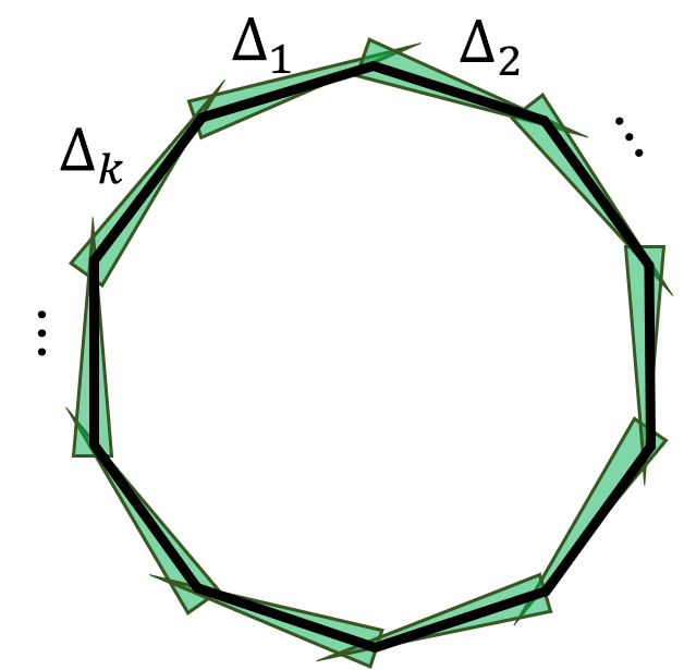
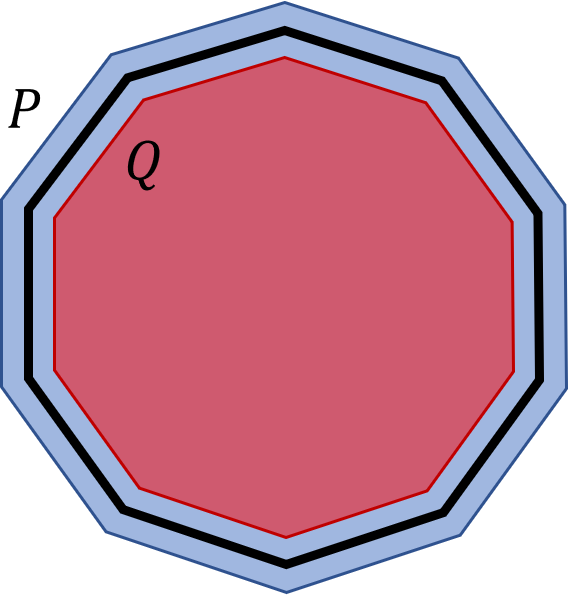
Figure 1: A comparison of Proposition 3.1, Theorem 3.2, and Theorem 3.3 in Example 3.4. (a) Let 𝒳𝒳\mathcal{X} be the boundary of a regular k𝑘k-gon in 2superscript2{\mathbb{R}}^{2}. (b) A triangle covering of 𝒳𝒳\mathcal{X} is given. Proposition 3.1 provides the network architecture 2σ3kσkMAX1superscript𝜎23𝑘superscript𝜎𝑘superscriptMAX12\stackrel{{\scriptstyle\sigma}}{{\rightarrow}}3k\stackrel{{\scriptstyle\sigma}}{{\rightarrow}}k\stackrel{{\scriptstyle\texttt{MAX}}}{{\rightarrow}}1. (c) Bε(𝒳)subscript𝐵𝜀𝒳B_{\varepsilon}(\mathcal{X}) can be covered by the difference of two k𝑘k-gon P𝑃P and Q𝑄Q. Then, Theorem 3.2 guarantees that a network with the architecture 2σ2kσ2σ2σ1superscript𝜎22𝑘superscript𝜎2superscript𝜎2superscript𝜎12\stackrel{{\scriptstyle\sigma}}{{\rightarrow}}2k\stackrel{{\scriptstyle\sigma}}{{\rightarrow}}2\stackrel{{\scriptstyle\sigma}}{{\rightarrow}}2\stackrel{{\scriptstyle\sigma}}{{\rightarrow}}1 can approximate 𝟙{𝒳}subscript1𝒳\mathbbm{1}_{\{\mathcal{X}\}}.
Example 3.4 (Comparison of Proposition 3.1, Theorem 3.2, and Theorem 3.3).

Let 𝒳𝒳\mathcal{X} be the boundary of a regular k𝑘k-gon in 2superscript2{\mathbb{R}}^{2} as shown in Figure 1(a). First, consider a convex polytope covering 𝒞𝒞\mathcal{C} that consists of k𝑘k green triangles in Figure 1(b). Proposition 3.1 shows that a three layer network with the architecture 2σ3kσkMAX1superscript𝜎23𝑘superscript𝜎𝑘superscriptMAX12\stackrel{{\scriptstyle\sigma}}{{\rightarrow}}3k\stackrel{{\scriptstyle\sigma}}{{\rightarrow}}k\stackrel{{\scriptstyle\texttt{MAX}}}{{\rightarrow}}1 can approximate 𝟙{𝒳}subscript1𝒳\mathbbm{1}_{\{\mathcal{X}\}}. Since 𝒳𝒳\mathcal{X} can be regarded as a simplicial 222-complex with k𝑘k facets, Theorem 3.3 provides a slightly better bound 2σ(3k12k)σkMAX1superscript𝜎23𝑘12𝑘superscript𝜎𝑘superscriptMAX12\stackrel{{\scriptstyle\sigma}}{{\rightarrow}}\left(3k-\left\lfloor\frac{1}{2}k\right\rfloor\right)\stackrel{{\scriptstyle\sigma}}{{\rightarrow}}k\stackrel{{\scriptstyle\texttt{MAX}}}{{\rightarrow}}1, but both networks still have O(k)𝑂𝑘O(k) widths for two hidden layers. However, from its special structure of 𝒳𝒳\mathcal{X}, it can be covered by difference of two solid k𝑘k-gons P𝑃P and Q𝑄Q (Figure 1(c)). Then, Theorem 3.2 provides a four-layer ReLU network with the architecture 2σ2kσ2σ2σ1superscript𝜎22𝑘superscript𝜎2superscript𝜎2superscript𝜎12\stackrel{{\scriptstyle\sigma}}{{\rightarrow}}2k\stackrel{{\scriptstyle\sigma}}{{\rightarrow}}2\stackrel{{\scriptstyle\sigma}}{{\rightarrow}}2\stackrel{{\scriptstyle\sigma}}{{\rightarrow}}1, which has only one O(k)𝑂𝑘O(k) width. This example helps understand the benefits of depth from a topological perspective, akin to the advantages of depth studied in previous works [3, 39, 41, 44, 45]. It is also important to note that the high number of neurons in the first layer is inevitable, as described in [12] and [46].

It is remarkable that our findings can be extended to various other neural network architectures. In Appendix A, we broaden our results to encompass deep ReLU networks (as seen in Corollary A.1) and networks using sigmoid activation function at last (as presented in Corollary A.2).

3.2.3 Upper bounds of widths in terms of Betti numbers

The Betti number is a key metric used in TDA to denote the number of k𝑘k-dimensional ‘holes’ in a data distribution. Owing to its homotopy invariance, Betti numbers are frequently employed to study the topological features of a given topological space. Interestingly, our prior results can be leveraged to ascertain a neural network architecture with width bounds defined in terms of the Betti numbers, given that the dataset 𝒳𝒳\mathcal{X} exhibits certain structural characteristics.

Specifically, Theorem 3.2 offers upper width bounds when 𝒳𝒳\mathcal{X} can be depicted as a difference between unions of convex sets. Consequently, if 𝒳𝒳\mathcal{X} is convex and only contains ‘convex-shaped holes’, we can derive a network width bound in relation to its Betti numbers. This concept is further explicated in the following theorem and example.

Theorem 3.5.

Suppose 𝒳d𝒳superscript𝑑\mathcal{X}\subset{\mathbb{R}}^{d} is a topological space obtained by removing some disjoint rectangular prisms from a d𝑑d-dimensional cuboid. Let β0,β1,,βdsubscript𝛽0subscript𝛽1subscript𝛽𝑑\beta_{0},\beta_{1},\cdots,\beta_{d} be the Betti numbers of 𝒳𝒳\mathcal{X}. Then for any ε>0𝜀0\varepsilon>0, there exists a four-layer ReLU network 𝒩𝒩\mathcal{N} with the architecture

dσ 2(d1+k=0d(k+1)βk)σ(k=0dβk)σ2σ1superscript𝜎𝑑2𝑑1superscriptsubscript𝑘0𝑑𝑘1subscript𝛽𝑘superscript𝜎superscriptsubscript𝑘0𝑑subscript𝛽𝑘superscript𝜎2superscript𝜎1\displaystyle d\;\stackrel{{\scriptstyle\sigma}}{{\rightarrow}}\;2\left(d-1+\sum_{k=0}^{d}(k+1)\beta_{k}\right)\;\stackrel{{\scriptstyle\sigma}}{{\rightarrow}}\;\left(\sum_{k=0}^{d}\beta_{k}\right)\stackrel{{\scriptstyle\sigma}}{{\rightarrow}}2\stackrel{{\scriptstyle\sigma}}{{\rightarrow}}1 (2)

such that 𝒩(d)=[0,1]𝒩superscript𝑑01\mathcal{N}({\mathbb{R}}^{d})=[0,1], 𝒩(𝐱)=1𝒩𝐱1\mathcal{N}({\bm{x}})=1\; for 𝐱𝒳𝐱𝒳{\bm{x}}\in\mathcal{X}, and 𝒩(𝐱)=0𝒩𝐱0\mathcal{N}({\bm{x}})=0\; for 𝐱Bε(𝒳)𝐱subscript𝐵𝜀𝒳{\bm{x}}\not\in B_{\varepsilon}(\mathcal{X}).

Proof Sketch.

Since each k𝑘k-dimensional hole is a rectangular prism, we can consider it as convex polytopes. The result is deduced from Theorem 3.2 by computing the required number of faces of polytopes. The full proof can be found in Appendix B. ∎

Refer to caption
(a)
Refer to caption
(b)
Refer to caption
(c)
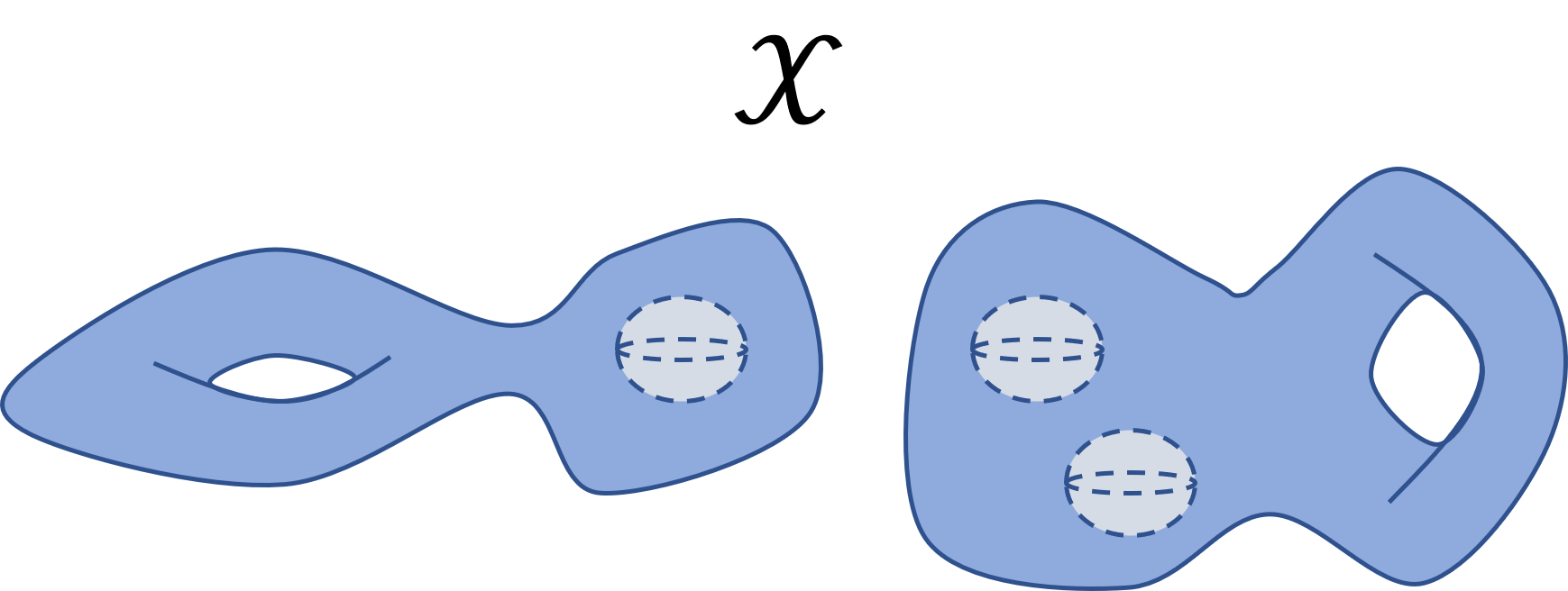
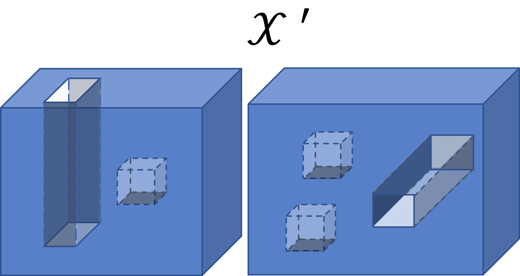
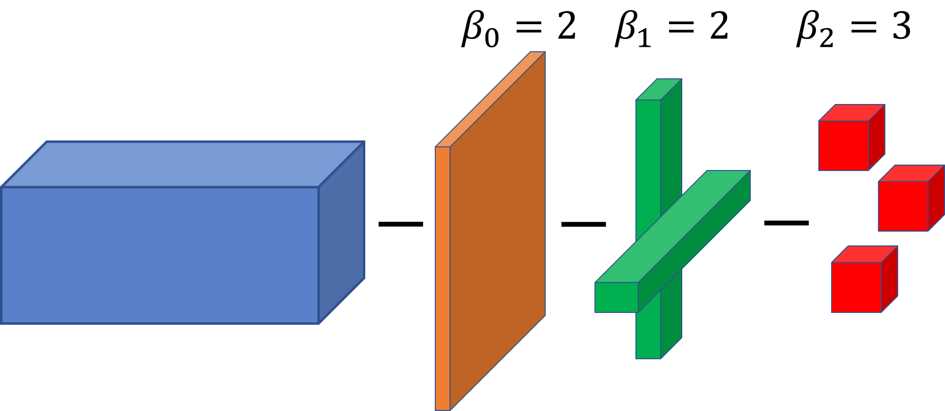
Figure 2: An illustration of the correlation between Betti numbers and the network architecture (Example 3.6). (a) A topological space 𝒳3𝒳superscript3\mathcal{X}\subset{\mathbb{R}}^{3} is given, whose Betti numbers are β0=β1=2subscript𝛽0subscript𝛽12\beta_{0}=\beta_{1}=2 and β2=3subscript𝛽23\beta_{2}=3. (b) A homotopy equivalent space 𝒳superscript𝒳\mathcal{X}^{\prime} is presented, obtained by removing several small cuboids from a larger one. (c) The removed cuboids from 𝒳superscript𝒳\mathcal{X}^{\prime} are shown. Theorem 3.5 demonstrates that a four-layer ReLU network with the architecture 3σ34σ7σ2σ1superscript𝜎334superscript𝜎7superscript𝜎2superscript𝜎13\stackrel{{\scriptstyle\sigma}}{{\rightarrow}}34\stackrel{{\scriptstyle\sigma}}{{\rightarrow}}7\stackrel{{\scriptstyle\sigma}}{{\rightarrow}}2\stackrel{{\scriptstyle\sigma}}{{\rightarrow}}1 can approximate 𝟙{𝒳}subscript1superscript𝒳\mathbbm{1}_{\{\mathcal{X}^{\prime}\}}.
Example 3.6.

Let 𝒳𝒳\mathcal{X} be a topological space in 3superscript3{\mathbb{R}}^{3} shown in Figure 2(a), which has three nonzero Betti numbers β0=β1=2subscript𝛽0subscript𝛽12\beta_{0}=\beta_{1}=2 and β2=3subscript𝛽23\beta_{2}=3. Then we can consider the homotopy equivalent topological space 𝒳3superscript𝒳superscript3\mathcal{X}^{\prime}\subset{\mathbb{R}}^{3} that satisfies the assumptions in Theorem 3.5: 𝒳superscript𝒳\mathcal{X}^{\prime} is obtained by ‘cutting out’ a plate (orange), ‘punching’ two rectangular prisms (green), and ‘hollowing out’ three small cubes (red) from a large cuboid (blue) as described in Figure 2(c). Then, Theorem 3.5 shows that a four-layer ReLU network with the architecture 3σ34σ7σ2σ1superscript𝜎334superscript𝜎7superscript𝜎2superscript𝜎13\stackrel{{\scriptstyle\sigma}}{{\rightarrow}}34\stackrel{{\scriptstyle\sigma}}{{\rightarrow}}7\stackrel{{\scriptstyle\sigma}}{{\rightarrow}}2\stackrel{{\scriptstyle\sigma}}{{\rightarrow}}1 can approximate 𝟙{𝒳}subscript1superscript𝒳\mathbbm{1}_{\{\mathcal{X}^{\prime}\}} arbitrarily closely.

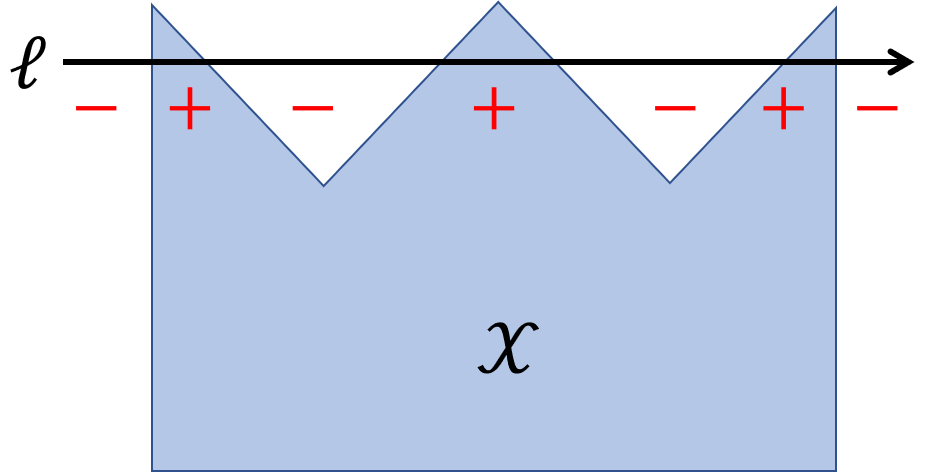
Theorem 3.5 and Example 3.6 illustrate how the Betti numbers of a topological space 𝒳𝒳\mathcal{X} can contribute to defining upper bounds for the widths of neural networks. However, it’s important to note that two homotopy equivalent spaces may require differing network architectures. In Proposition C.4, we prove that the indicator function over a crown-shaped topological space (Figure 5(a)) in 2superscript2{\mathbb{R}}^{2} cannot be approximated by a two-layer ReLU network with the architecture 2σ31superscript𝜎2312\stackrel{{\scriptstyle\sigma}}{{\rightarrow}}3\rightarrow 1, while a triangle can be approximated by Proposition 3.1. Since these two spaces have the same Betti numbers β0=1subscript𝛽01\beta_{0}=1, this example suggests that a neural network architecture cannot be solely determined by Betti numbers.

Nevertheless, Theorem 3.5 provides an upper bound on the widths of four-layer ReLU networks in terms of Betti numbers of 𝒳𝒳\mathcal{X}, under the conditions stipulated. This is another novel result linking the topological characteristics of a dataset with upper bounds on widths. It is worth noting that similar results can be achieved when the cuboid assumptions in Theorem 3.5 are modified to other convex polytopes, using the same proof strategy.

We further elaborate on the topic of network architecture. Intriguingly, the sum of Betti numbers k=0dβksuperscriptsubscript𝑘0𝑑subscript𝛽𝑘\sum_{k=0}^{d}\beta_{k} that appears in the third layer in (2) is termed the topological complexity of 𝒳𝒳\mathcal{X}. This quantity is recognized as a measure of the complexity of a given topological space [32]. This value has connections with other fields, for example, it has some lower and upper bounds from Morse theory [31] and Gromov’s Betti number Theorem [11]. In the context of topological data analysis, consider a C̆ech complex constructed on a dataset 𝒳𝒳\mathcal{X} consisting of n𝑛n points, using a filtration parameter ε𝜀\varepsilon. Its topological complexity fluctuates from n𝑛n (when ε=0𝜀0\varepsilon=0) to 111 (when ε>diam(𝒳)𝜀diam𝒳\varepsilon>\text{diam}(\mathcal{X})) as ε𝜀\varepsilon increases. This implies that the architecture in Theorem 3.5 is dictated by the filtration number ε𝜀\varepsilon, which controls the topological structure of the given dataset. We believe this approach could inspire novel investigative methods in TDA, which we propose as an avenue for future research.

4 Universal Approximation Property of Three-Layer ReLU Networks

In the preceding section, we demonstrated how indicator functions over certain topological spaces can be approximated by three-layer neural networks. Interestingly, this topological result has an application in proving the Universal Approximation Property (UAP) of three-layer ReLU networks. Moreover, we can derive upper bounds on the widths in three-layer ReLU networks for approximating Lipschitz functions. We present this result in the upcoming theorem.

Theorem 4.1.

Let dx,dysubscript𝑑𝑥subscript𝑑𝑦d_{x},d_{y}\in{\mathbb{N}} and p1𝑝1p\geq 1. Then, the set of three-layer ReLU networks is dense in Lp(dx,[0,1]dy)superscript𝐿𝑝superscriptsubscript𝑑𝑥superscript01subscript𝑑𝑦L^{p}({\mathbb{R}}^{d_{x}},[0,1]^{d_{y}}). Furthermore, let f:dx[0,1]dy:𝑓superscriptsubscript𝑑𝑥superscript01subscript𝑑𝑦f:{\mathbb{R}}^{d_{x}}\rightarrow[0,1]^{d_{y}} be a compactly supported Lipschitz function. Then for any ε>0𝜀0\varepsilon>0, there exists a three-layer ReLU network 𝒩𝒩\mathcal{N} with the architecture

dxσ(2ndxdy)σ(ndy)dysuperscript𝜎subscript𝑑𝑥2𝑛subscript𝑑𝑥subscript𝑑𝑦superscript𝜎𝑛subscript𝑑𝑦subscript𝑑𝑦\displaystyle d_{x}\;\stackrel{{\scriptstyle\sigma}}{{\rightarrow}}\;(2nd_{x}d_{y})\;\stackrel{{\scriptstyle\sigma}}{{\rightarrow}}\;(nd_{y})\;\rightarrow d_{y}

such that 𝒩fLp(dx)<εsubscriptnorm𝒩𝑓superscript𝐿𝑝superscriptsubscript𝑑𝑥𝜀\left\|\mathcal{N}-f\right\|_{L^{p}({\mathbb{R}}^{d_{x}})}<\varepsilon. Here, n=O(εdx)𝑛𝑂superscript𝜀subscript𝑑𝑥n=O(\varepsilon^{-d_{x}}).

Proof Sketch.

The first assertion is a consequence of the second one. Regarding the second assertion, note that fsuperscript𝑓f^{*}, being Lipschitz, is continuous and Riemann integrable. Consequently, we can construct a linear combination of indicator functions that approximates fsuperscript𝑓f^{*}, which are known as simple functions in Lebesgue theory [38]. Each of these indicator functions can be implemented by a three-layer ReLU network using Proposition 3.1. The complete proof can be found in Appendix B. ∎

Theorem 4.1 makes two assertions. The first one affirms that the set of three-layer ReLU networks is dense in Lp(dx,[0,1]dy)superscript𝐿𝑝superscriptsubscript𝑑𝑥superscript01subscript𝑑𝑦L^{p}({\mathbb{R}}^{d_{x}},[0,1]^{d_{y}}), aligning with the findings presented in [45]. Considering that we have also demonstrated that the set of two-layer ReLU networks cannot universally approximate a compactly supported function (as per Proposition 1.1), we can conclude that the minimum depth of DNNs to achieve universal approximation in Lp(dx)superscript𝐿𝑝superscriptsubscript𝑑𝑥L^{p}({\mathbb{R}}^{d_{x}}) is precisely 3. This conclusion refines the results shown in [45]. Moreover, while [45] merely demonstrates the possibility of approximating functions using three-layer ReLU networks, the second assertion of Theorem 4.1 provides upper bounds on the widths, which are O(εdx)𝑂superscript𝜀subscript𝑑𝑥O(\varepsilon^{-d_{x}}), when the function to be approximated, fsuperscript𝑓f^{*}, is Lipschitz and compactly supported. As far as we are aware, this is the first work to present an upper bound on the width of three-layer ReLU networks for UAP.

These findings open a potential path to extend our topological results. We expect that for certain classes of functions, the width bounds could be reduced by adding more layers to the network, as demonstrated in Theorem 3.2 and Example 3.4. However, we leave this as an area for future research.

5 Experimental Results

In Section 3, we introduced a construction for three or four-layer neural networks that can approximate 𝟙{𝒳}subscript1𝒳\mathbbm{1}_{\{\mathcal{X}\}} for any given topological space 𝒳𝒳\mathcal{X} with a sufficient degree of accuracy. Naturally, this leads us to the question of whether these networks can be produced using a gradient method. While most prior theoretical studies concerning the existence of neural networks have not included experimental verification [22, 23, 25, 34], the issue of experimental verification remains an important one, as noted in [44]. In this section, we will provide experimental evidence that gradient descent can indeed converge to the neural networks that we constructed in Section 3.

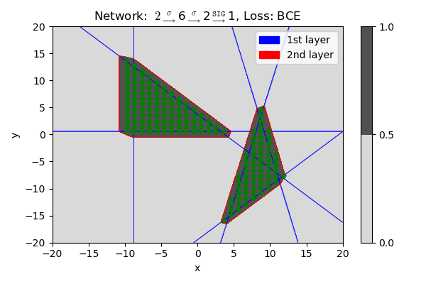
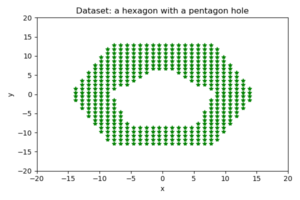
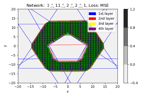
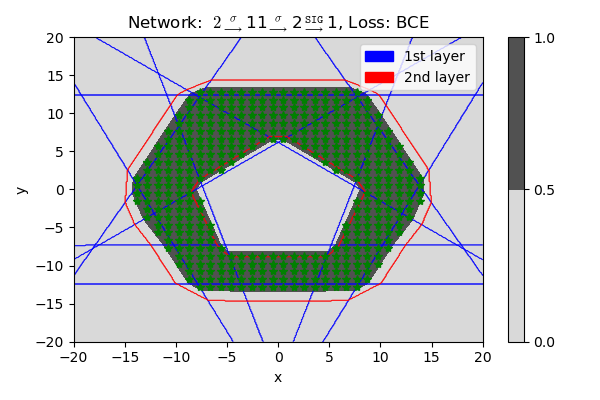
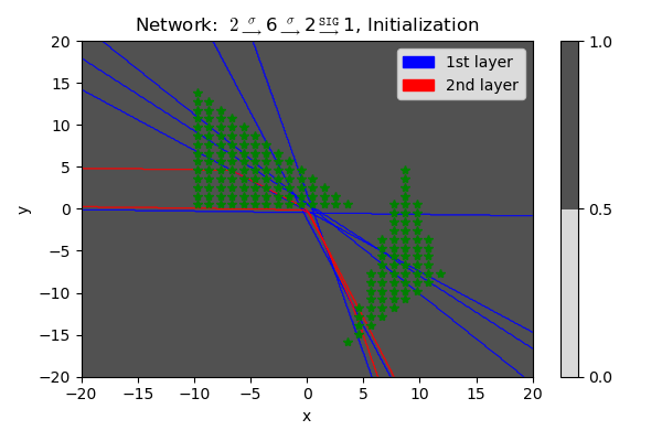
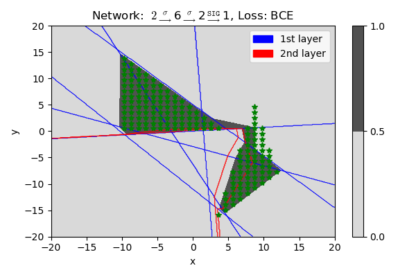
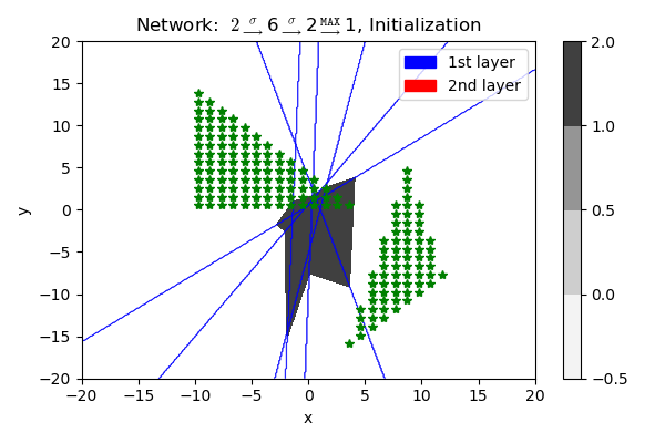
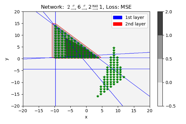
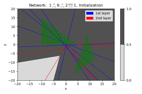
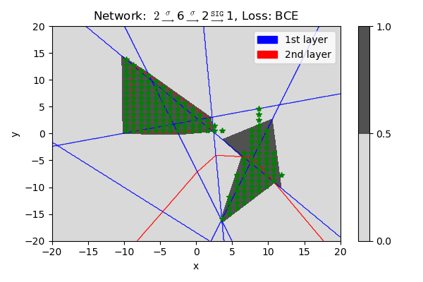
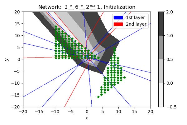
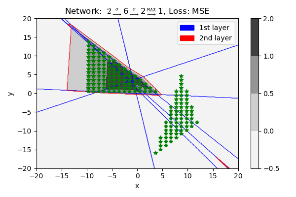
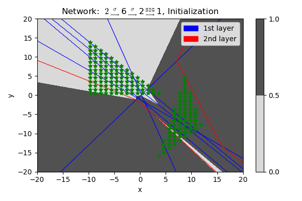
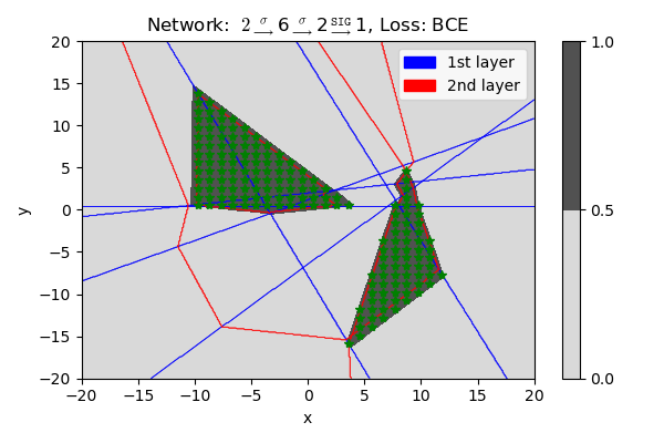
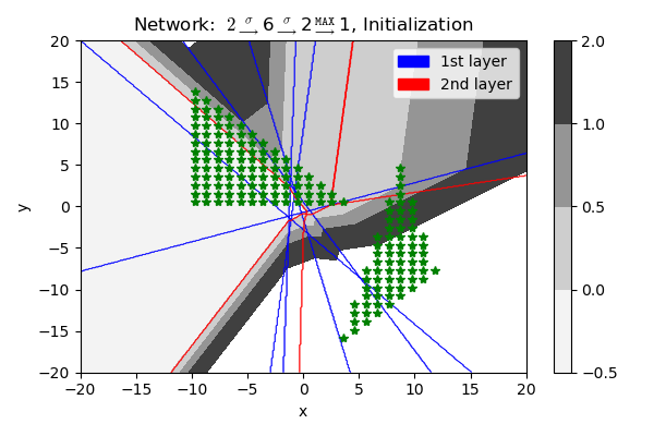
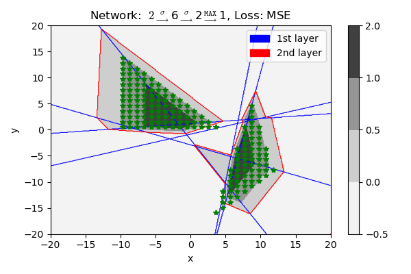
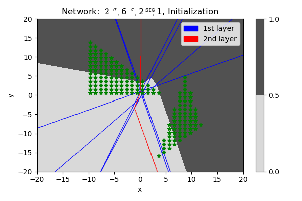
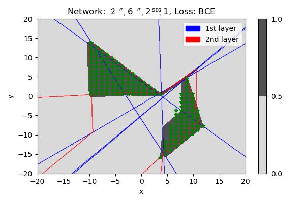
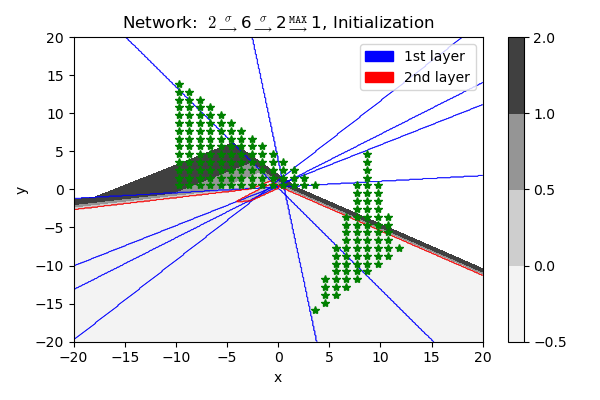
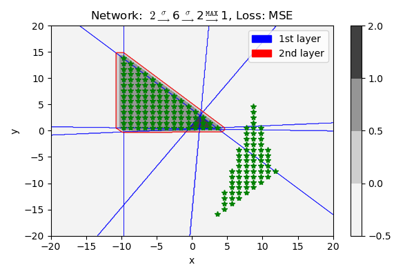
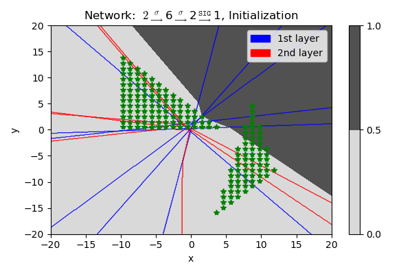
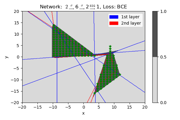
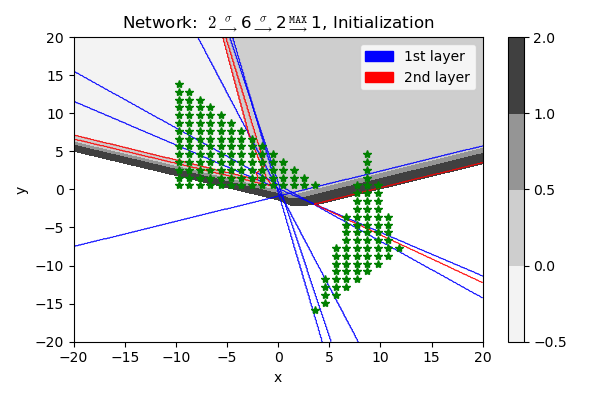
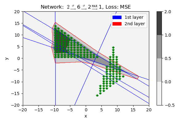
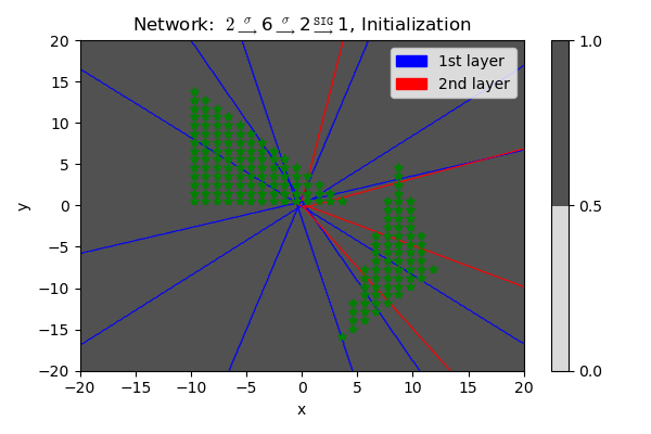
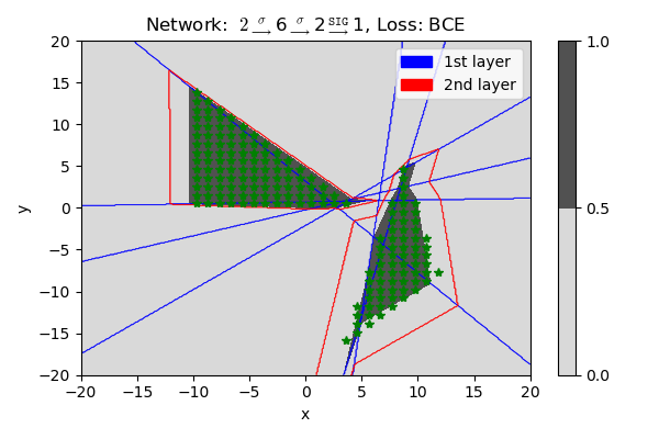
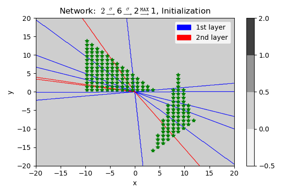
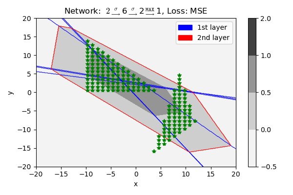
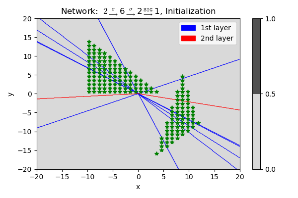
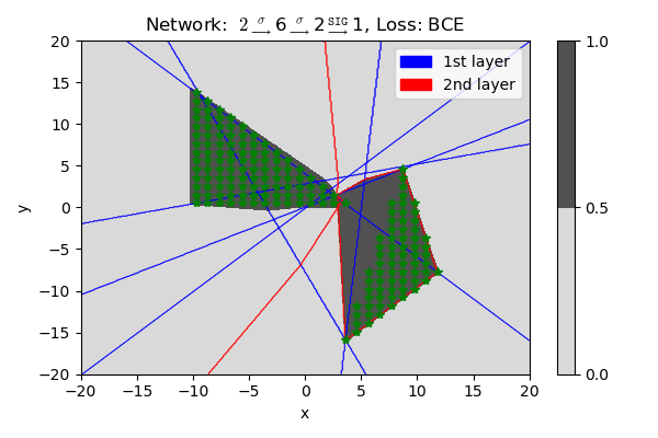
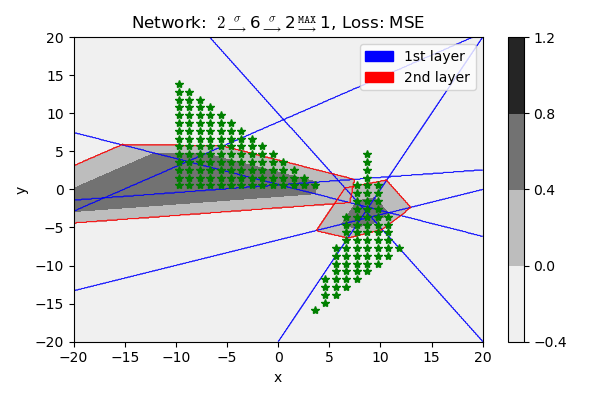
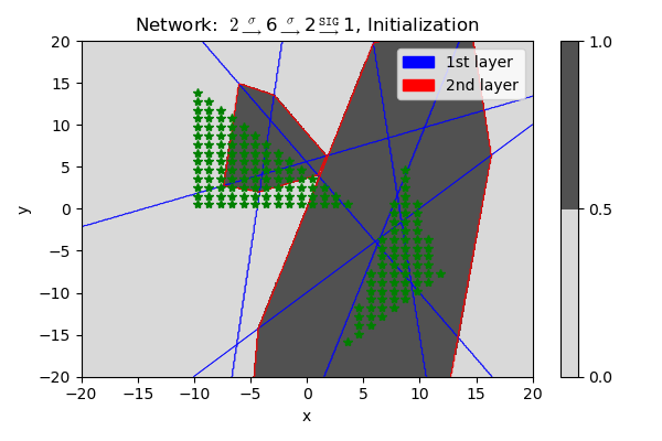
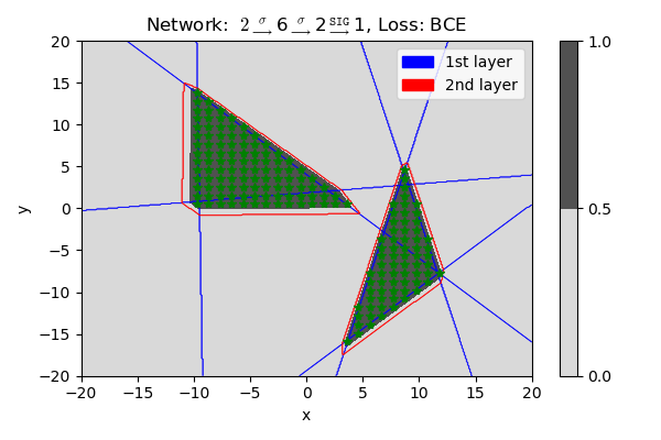
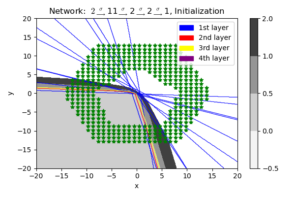
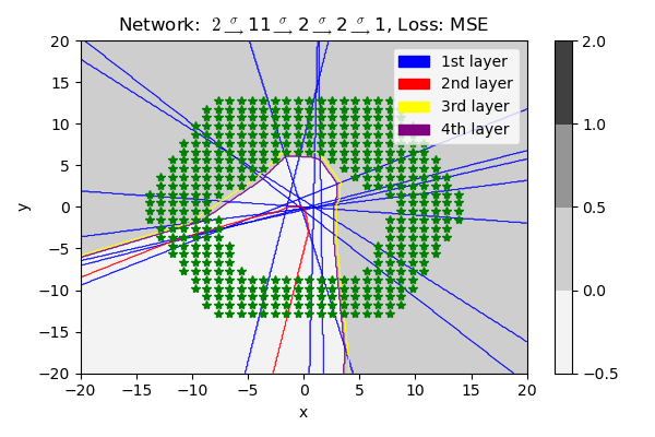
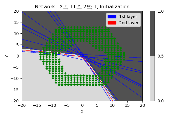
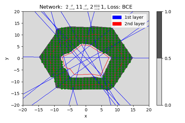
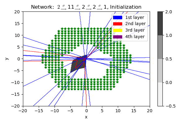
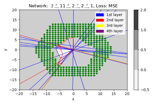
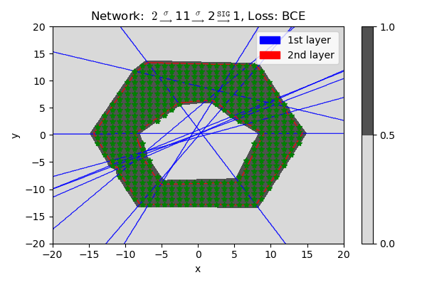
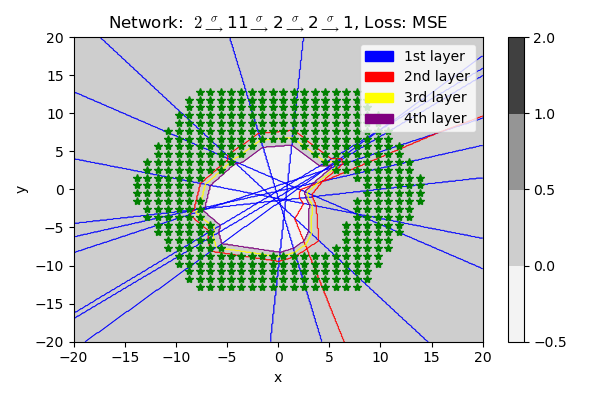
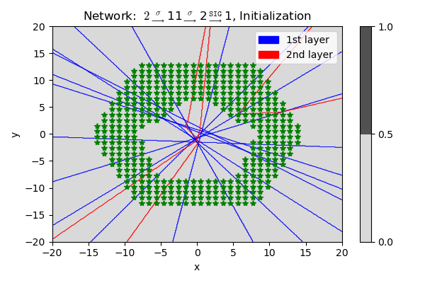
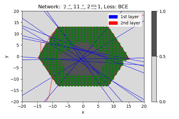
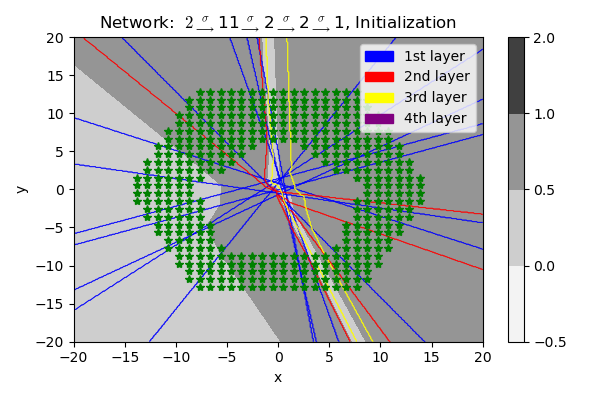
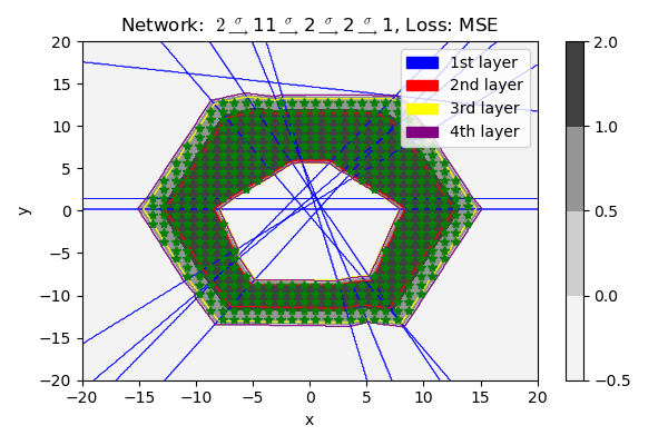
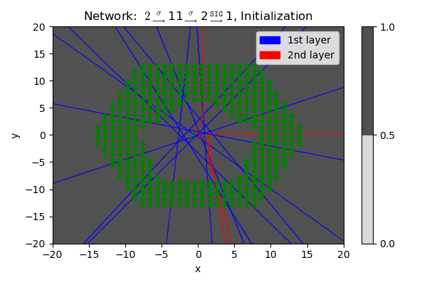
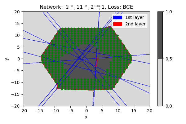
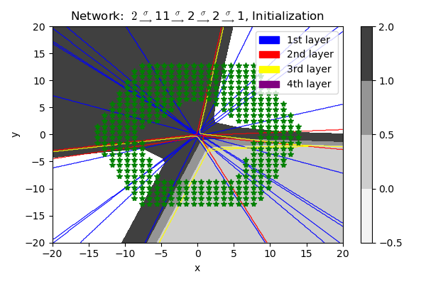
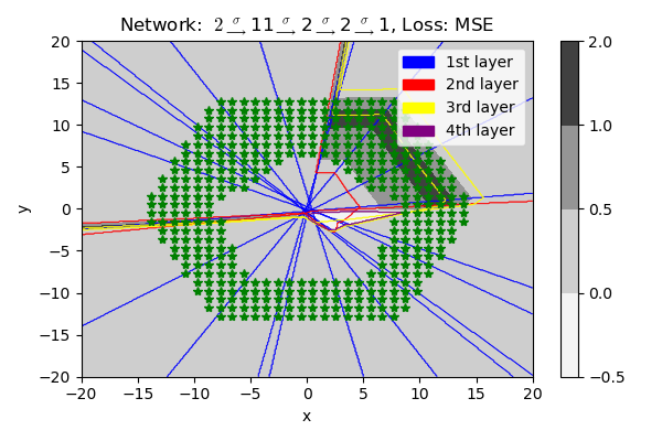
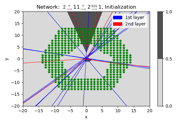
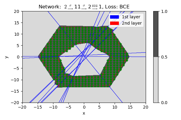
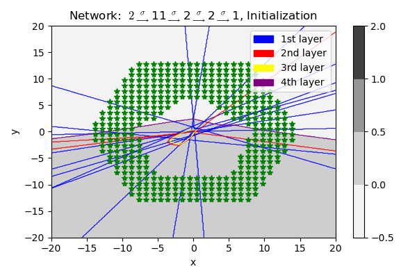
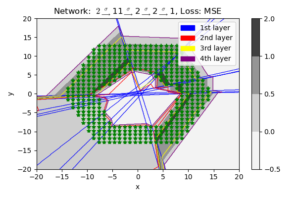
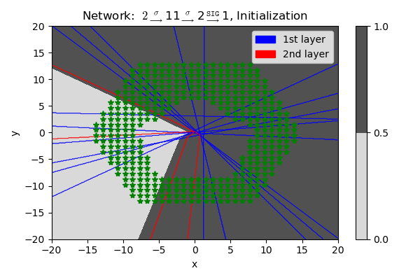
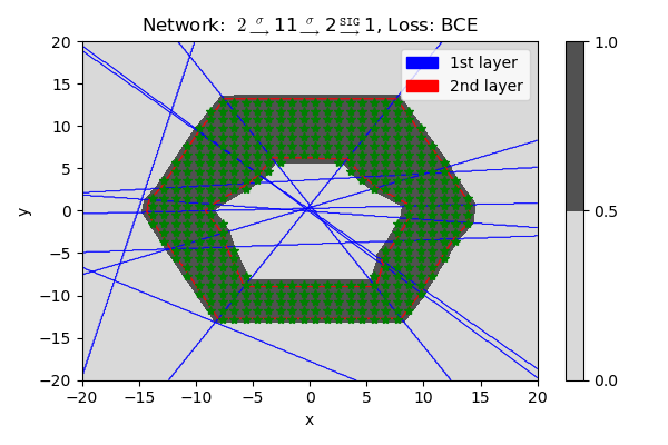
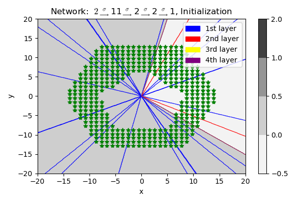
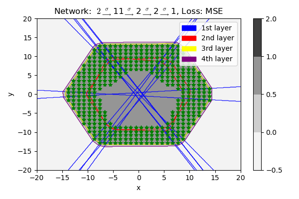
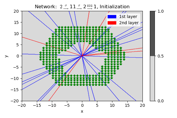
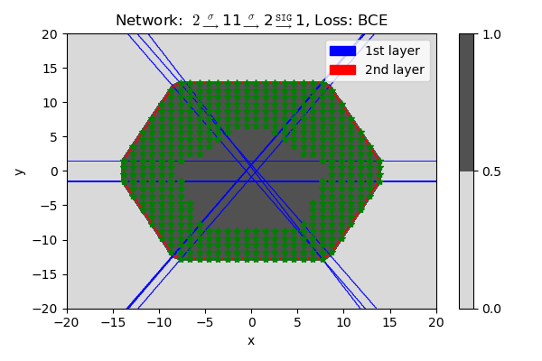
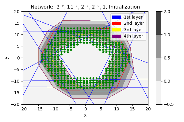
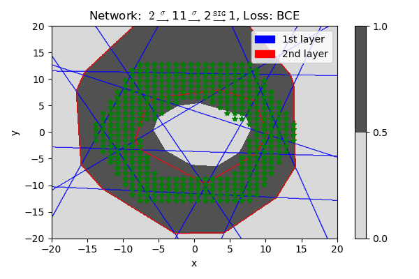
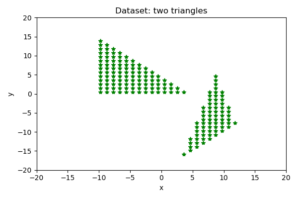
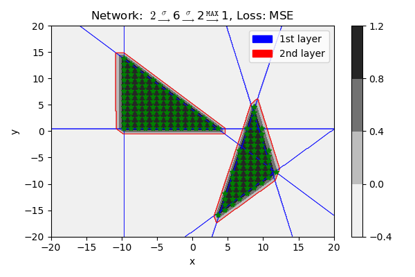
We consider two illustrative manifolds, 𝒳1subscript𝒳1\mathcal{X}_{1} and 𝒳2subscript𝒳2\mathcal{X}_{2}, depicted in Figure 3(a) and (d) respectively. The first compact set 𝒳1subscript𝒳1\mathcal{X}_{1} is a simplicial 222-complex in 2superscript2{\mathbb{R}}^{2} comprised of two triangles. The second compact set 𝒳2subscript𝒳2\mathcal{X}_{2} is a hexagon with a pentagonal hole, which is not a simplicial complex but a compact manifold. The datasets are constructed by selecting 1600 equidistant lattice points in the domain [20,20]×[20,20]220202020superscript2[-20,20]\times[-20,20]\subset{\mathbb{R}}^{2}, where each point has label ‘111’ if it lies on the manifold 𝒳isubscript𝒳𝑖\mathcal{X}_{i}, and ‘00’ otherwise. We undertake both regression and classification tasks, using mean square error (MSE) loss and binary cross entropy (BCE) loss respectively. For the BCE loss task, we adhere to the architecture proposed in Corollary A.2 to ensure trainability. We employ the gradient descent algorithm for training our networks. For a clearer visualization of weight vectors in each layer, we plot the lines of vanishing points for each layer in blue (1st layer), red (2nd layer), etc. The grayscale color denotes the output range of the trained network.
Refer to caption
(a)
Refer to caption
(b)
Refer to caption
(c)
Refer to caption
(d)
Refer to caption
(e)
Refer to caption
(f)
Figure 3: Experimental verification of convergence of gradient descent. (a) and (d) exhibit the shape of two data manifolds, which are ‘two triangles’ and ‘a hexagon with a pentagon hole’. (b) and (e) show the converged networks by gradient descent, when the loss function is given by the mean square error (MSE) loss. Similarly, (e) and (f) show the results for the binary cross entropy (BCE) loss. These results verify that gradient descent indeed converges to the networks we proposed in Section 3.

For the first data manifold 𝒳1subscript𝒳1\mathcal{X}_{1}, Theorem 3.3 suggests that a network with the architecture 2σ6σ2MAX1superscript𝜎26superscript𝜎2superscriptMAX12\stackrel{{\scriptstyle\sigma}}{{\rightarrow}}6\stackrel{{\scriptstyle\sigma}}{{\rightarrow}}2\stackrel{{\scriptstyle\texttt{MAX}}}{{\rightarrow}}1 can precisely represent 𝟙{𝒳1}subscript1subscript𝒳1\mathbbm{1}_{\{\mathcal{X}_{1}\}}. As depicted in Figure 3(b), the trained network indeed converges exactly to the network proposed in the theorem under MSE loss. The weight vectors in the first layer encapsulate the two triangles, reflecting the topology of 𝒳1subscript𝒳1\mathcal{X}_{1}. A similar result can be observed for a network with the architecture 2σ6σ2SIG1superscript𝜎26superscript𝜎2superscriptSIG12\stackrel{{\scriptstyle\sigma}}{{\rightarrow}}6\stackrel{{\scriptstyle\sigma}}{{\rightarrow}}2\stackrel{{\scriptstyle\texttt{SIG}}}{{\rightarrow}}1, as suggested by Corollary A.2. For the second data manifold 𝒳2subscript𝒳2\mathcal{X}_{2}, Theorem 3.2 suggests that a network with the architecture 2σ11σ2σ2σ1superscript𝜎211superscript𝜎2superscript𝜎2superscript𝜎12\stackrel{{\scriptstyle\sigma}}{{\rightarrow}}11\stackrel{{\scriptstyle\sigma}}{{\rightarrow}}2\stackrel{{\scriptstyle\sigma}}{{\rightarrow}}2\stackrel{{\scriptstyle\sigma}}{{\rightarrow}}1 can fit this manifold, and Figure 3(e) verifies this under MSE loss. The architecture 2σ11σ2SIG1superscript𝜎211superscript𝜎2superscriptSIG12\stackrel{{\scriptstyle\sigma}}{{\rightarrow}}11\stackrel{{\scriptstyle\sigma}}{{\rightarrow}}2\stackrel{{\scriptstyle\texttt{SIG}}}{{\rightarrow}}1 also converges to the network proposed in Corollary A.2, as shown in Figure 3(f). More specifically, the eleven weight vectors in the first layer align with the eleven boundaries of the outer hexagon and the inner pentagon, with two neurons in the second layer encapsulating each polygon.

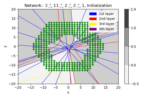
These experimental results provide evidence that the networks proposed in Section 3 can indeed be reached as the global minima by gradient descent, under both MSE loss and BCE loss. However, we must stress the importance of initialization. Although we observe successful convergence to the expected networks, the results are heavily dependent on the initialization. For instance, under random initialization, it is known that all neurons in a layer may ‘die’ at initialization with a nonzero probability [27], leading to a poor network performance. We provide further experimental results concerning different initializations in Appendix D. The key takeaway from this section is that the networks proposed in Section 3 can indeed be reached by gradient descent, a fact not demonstrated by prior studies on UAP, even in the context of toy examples.

6 Conclusions

While many previous studies have explored the universal approximation property of DNNs, they have largely overlooked the connection with the topological features of datasets. In this paper, we have addressed this gap by providing data topology-dependent upper bounds on the width of DNNs. We have shown that for a dataset 𝒳𝒳\mathcal{X} that can be tightly covered by convex polytopes, a three-layer network architecture can be derived to approximate the indicator function 𝟙{𝒳}subscript1𝒳\mathbbm{1}_{\{\mathcal{X}\}}. We also extended this to four-layer ReLU networks for 𝒳𝒳\mathcal{X} that can be covered by the difference of two unions of convex polytopes. We further generalized this to simplicial m𝑚m-complexes and demonstrated the construction of a three-layer neural network with ReLU activation and max pooling operation. Imposing further assumptions on 𝒳𝒳\mathcal{X}, we proposed the architecture of four-layer ReLU networks whose widths are bounded in terms of Betti numbers, a novel result in this field. Finally, we demonstrated that to approximate a compactly supported Lipschitz function in dxsuperscriptsubscript𝑑𝑥{\mathbb{R}}^{d_{x}} by a three-layer ReLU network under an ε𝜀\varepsilon error, a width of O(εdx)𝑂superscript𝜀subscript𝑑𝑥O(\varepsilon^{-d_{x}}) is sufficient. Through our experiments, we showed that gradient descent indeed converges to the networks we proposed.

Limitations and Future Works

There are several limitations. Firstly, although we experimentally showed convergence to the constructed network, we did not provide a rigorous guarantee for this convergence here. To overcome this and to ensure both existence and convergence, it would be valuable to prove a convergence result under specific conditions. Secondly, further research is needed to investigate the relationship between the network architecture and Betti numbers of the given topological spaces. The results in Theorem 3.5 suggest that it may be possible to expand our findings or reduce some assumptions on the given topological space. Since Betti numbers are commonly used features to characterize topological features of data manifolds in Topological Data Analysis (TDA), we believe that this line of research could yield significant insights.

References

  • [1] Adrian Barbu and Hongyu Mou. The compact support neural network. Sensors, 21(24):8494, 2021.
  • [2] Andrew R Barron. Universal approximation bounds for superpositions of a sigmoidal function. IEEE Transactions on Information theory, 39(3):930–945, 1993.
  • [3] Kaifeng Bu, Yaobo Zhang, and Qingxian Luo. Depth-width trade-offs for neural networks via topological entropy. arXiv preprint arXiv:2010.07587, 2020.
  • [4] Gunnar Carlsson. Topological pattern recognition for point cloud data. Acta Numerica, 23:289–368, 2014.
  • [5] Jeremy EJ Cohen, Todd Huster, and Ra Cohen. Universal lipschitz approximation in bounded depth neural networks. arXiv preprint arXiv:1904.04861, 2019.
  • [6] George Cybenko. Approximation by superpositions of a sigmoidal function. Mathematics of control, signals and systems, 2(4):303–314, 1989.
  • [7] Ronen Eldan and Ohad Shamir. The power of depth for feedforward neural networks. In Conference on learning theory, pages 907–940. PMLR, 2016.
  • [8] Stanislav Fort, Ekin Dogus Cubuk, Surya Ganguli, and Samuel S Schoenholz. What does a deep neural network confidently perceive? the effective dimension of high certainty class manifolds and their low confidence boundaries. arXiv preprint arXiv:2210.05546, 2022.
  • [9] Xavier Glorot and Yoshua Bengio. Understanding the difficulty of training deep feedforward neural networks. In Proceedings of the thirteenth international conference on artificial intelligence and statistics, pages 249–256. JMLR Workshop and Conference Proceedings, 2010.
  • [10] Ian Goodfellow, Yoshua Bengio, and Aaron Courville. Deep learning. MIT press, 2016.
  • [11] Michael Gromov. Curvature, diameter and betti numbers. Commentarii Mathematici Helvetici, 56:179–195, 1981.
  • [12] William H Guss and Ruslan Salakhutdinov. On characterizing the capacity of neural networks using algebraic topology. arXiv preprint arXiv:1802.04443, 2018.
  • [13] Mustafa Hajij and Kyle Istvan. A topological framework for deep learning. arXiv preprint arXiv:2008.13697, 2020.
  • [14] Mustafa Hajij and Kyle Istvan. Topological deep learning: Classification neural networks. arXiv preprint arXiv:2102.08354, 2021.
  • [15] Boris Hanin. Universal function approximation by deep neural nets with bounded width and relu activations. Mathematics, 7(10):992, 2019.
  • [16] Juncai He, Lin Li, Jinchao Xu, and Chunyue Zheng. Relu deep neural networks and linear finite elements. arXiv preprint arXiv:1807.03973, 2018.
  • [17] Kaiming He, Xiangyu Zhang, Shaoqing Ren, and Jian Sun. Delving deep into rectifiers: Surpassing human-level performance on imagenet classification. In Proceedings of the IEEE international conference on computer vision, pages 1026–1034, 2015.
  • [18] Robert Hecht-Nielsen. Kolmogorov’s mapping neural network existence theorem. In Proceedings of the international conference on Neural Networks, volume 3, pages 11–14. IEEE Press New York, NY, USA, 1987.
  • [19] Felix Hensel, Michael Moor, and Bastian Rieck. A survey of topological machine learning methods. Frontiers in Artificial Intelligence, 4:681108, 2021.
  • [20] Christoph Hertrich, Amitabh Basu, Marco Di Summa, and Martin Skutella. Towards lower bounds on the depth of relu neural networks. Advances in Neural Information Processing Systems, 34:3336–3348, 2021.
  • [21] Kurt Hornik. Approximation capabilities of multilayer feedforward networks. Neural networks, 4(2):251–257, 1991.
  • [22] Changcun Huang. Relu networks are universal approximators via piecewise linear or constant functions. Neural Computation, 32(11):2249–2278, 2020.
  • [23] Changcun Huang. Theoretical exploration of solutions of feedforward relu networks. arXiv preprint arXiv:2202.01919, 2022.
  • [24] Geonho Hwang, Myungjoo Kang, et al. Minimal width for universal property of deep rnn. arXiv preprint arXiv:2211.13866, 2022.
  • [25] Vugar Ismailov. A three layer neural network can represent any multivariate function. arXiv preprint arXiv:2012.03016, 2020.
  • [26] Anastasis Kratsios and Behnoosh Zamanlooy. Do relu networks have an edge when approximating compactly-supported functions? Transactions on Machine Learning Research, 2022.
  • [27] Lu Lu, Yeonjong Shin, Yanhui Su, and George Em Karniadakis. Dying relu and initialization: Theory and numerical examples. arXiv preprint arXiv:1903.06733, 2019.
  • [28] Pek Y Lum, Gurjeet Singh, Alan Lehman, Tigran Ishkanov, Mikael Vejdemo-Johansson, Muthu Alagappan, John Carlsson, and Gunnar Carlsson. Extracting insights from the shape of complex data using topology. Scientific reports, 3(1):1–8, 2013.
  • [29] Diane Maclagan and Bernd Sturmfels. Introduction to tropical geometry, volume 161. American Mathematical Society, 2021.
  • [30] German Magai and Anton Ayzenberg. Topology and geometry of data manifold in deep learning. arXiv preprint arXiv:2204.08624, 2022.
  • [31] John Willard Milnor, Michael Spivak, Robert Wells, and Robert Wells. Morse theory. Princeton university press, 1963.
  • [32] Gregory Naitzat, Andrey Zhitnikov, and Lek-Heng Lim. Topology of deep neural networks. The Journal of Machine Learning Research, 21(1):7503–7542, 2020.
  • [33] Monica Nicolau, Arnold J Levine, and Gunnar Carlsson. Topology based data analysis identifies a subgroup of breast cancers with a unique mutational profile and excellent survival. Proceedings of the National Academy of Sciences, 108(17):7265–7270, 2011.
  • [34] Sejun Park, Chulhee Yun, Jaeho Lee, and Jinwoo Shin. Minimum width for universal approximation. arXiv preprint arXiv:2006.08859, 2020.
  • [35] Dmytro Perekrestenko, Philipp Grohs, Dennis Elbrächter, and Helmut Bölcskei. The universal approximation power of finite-width deep relu networks. arXiv preprint arXiv:1806.01528, 2018.
  • [36] Dmytro Perekrestenko, Stephan Müller, and Helmut Bölcskei. Constructive universal high-dimensional distribution generation through deep relu networks. In International Conference on Machine Learning, pages 7610–7619. PMLR, 2020.
  • [37] Allan Pinkus. Approximation theory of the mlp model in neural networks. Acta numerica, 8:143–195, 1999.
  • [38] Walter Rudin et al. Principles of mathematical analysis, volume 3. McGraw-hill New York, 1976.
  • [39] Itay Safran and Ohad Shamir. Depth-width tradeoffs in approximating natural functions with neural networks. In International conference on machine learning, pages 2979–2987. PMLR, 2017.
  • [40] Linhao Song, Jun Fan, Di-Rong Chen, and Ding-Xuan Zhou. Approximation of nonlinear functionals using deep relu networks. arXiv preprint arXiv:2304.04443, 2023.
  • [41] Matus Telgarsky. Benefits of depth in neural networks. In Conference on learning theory, pages 1517–1539. PMLR, 2016.
  • [42] Saket Tiwari and George Konidaris. Effects of data geometry in early deep learning. arXiv preprint arXiv:2301.00008, 2022.
  • [43] Ilya Trofimov, Daniil Cherniavskii, Eduard Tulchinskii, Nikita Balabin, Evgeny Burnaev, and Serguei Barannikov. Learning topology-preserving data representations. arXiv preprint arXiv:2302.00136, 2023.
  • [44] Gal Vardi, Gilad Yehudai, and Ohad Shamir. Width is less important than depth in relu neural networks. In Conference on Learning Theory, pages 1249–1281. PMLR, 2022.
  • [45] Ming-Xi Wang and Yang Qu. Approximation capabilities of neural networks on unbounded domains. Neural Networks, 145:56–67, 2022.
  • [46] Ji Yang, Lu Sang, and Daniel Cremers. Dive into layers: Neural network capacity bounding using algebraic geometry. arXiv preprint arXiv:2109.01461, 2021.
  • [47] Ali Zia, Abdelwahed Khamis, James Nichols, Zeeshan Hayder, Vivien Rolland, and Lars Petersson. Topological deep learning: A review of an emerging paradigm. arXiv preprint arXiv:2302.03836, 2023.

Appendix

Appendix A Extension to Deep ReLU Networks and Cross Entropy Loss

In Section 3, we presented a variety of three and four-layer neural networks utilizing ReLU activation and max pooling operations. In this section, due to its unique structure, we extend our discussion to other neural network architectures. Particularly, we focus on networks that exclusively use ReLU activations, which are prevalent and effective in practical applications.

Interestingly, the principle outlined in Lemma C.2 enables us to replace the MAX operation in the final layer with an additional ReLU layer. This revelation lays the groundwork for the following corollary, which directly stems from Proposition 3.1 and Theorem 3.3

Corollary A.1 (Four-layer ReLU networks).

The three-layer neural network in Proposition 3.1 or Theorem 3.3 can be changed to a four-layer ReLU network with the architecture dσd1σd2σ11superscript𝜎𝑑subscript𝑑1superscript𝜎subscript𝑑2superscript𝜎11d\stackrel{{\scriptstyle\sigma}}{{\rightarrow}}d_{1}\stackrel{{\scriptstyle\sigma}}{{\rightarrow}}d_{2}\stackrel{{\scriptstyle\sigma}}{{\rightarrow}}1\rightarrow 1, where d1subscript𝑑1d_{1} and d2subscript𝑑2d_{2} are exhibited in the proposition or theorem.

Proof.

Consider the three-layer neural network proposed in Proposition 3.1 or Theorem 3.3 which has the architecture dσd1σd2MAX1superscript𝜎𝑑subscript𝑑1superscript𝜎subscript𝑑2superscriptMAX1d\stackrel{{\scriptstyle\sigma}}{{\rightarrow}}d_{1}\stackrel{{\scriptstyle\sigma}}{{\rightarrow}}d_{2}\stackrel{{\scriptstyle\texttt{MAX}}}{{\rightarrow}}1. Let a1,,ad2subscript𝑎1subscript𝑎subscript𝑑2a_{1},\cdots,a_{d_{2}} be the input of the last layer, thus the output of the second layer. Since a1,,ad2[0,1]subscript𝑎1subscript𝑎subscript𝑑201a_{1},\cdots,a_{d_{2}}\in[0,1] from the construction, we get MAX(a1,,ak)=1σ(1a1ak)MAXsubscript𝑎1subscript𝑎𝑘1𝜎1subscript𝑎1subscript𝑎𝑘\texttt{MAX}(a_{1},\cdots,a_{k})=1-\sigma(1-a_{1}-\cdots-a_{k}). This completes the proof. ∎

We now turn our attention to neural networks trained under binary cross entropy (BCE) loss. For a single pair of data 𝒙𝒙{\bm{x}} and its corresponding label y𝑦y, the BCE loss is defined as (𝒙,y):=ylog(𝒩(𝒙))+(1y)log(1𝒩(𝒙))assign𝒙𝑦𝑦𝒩𝒙1𝑦1𝒩𝒙\ell({\bm{x}},y):=y\log(\mathcal{N}({\bm{x}}))+(1-y)\log(1-\mathcal{N}({\bm{x}})). Hence, during training, the output of the neural network must neither be zero nor exceed 111. This requirement is the primary reason classifiers utilize the sigmoid activation function SIG(x):=11+exassignSIG𝑥11superscript𝑒𝑥\texttt{SIG}(x):=\frac{1}{1+e^{-x}}.

In light of this, we extend our findings to accommodate a network that employs sigmoid activation in the final layer. This adjustment can be readily achieved using our previous results, as detailed in Corollary A.1. Notably, this expansion does not necessitate extra layers, unlike in Corollary A.1. The outcome is presented in the subsequent corollary.

Corollary A.2 (Cross entropy loss).

Let 𝒩𝒩\mathcal{N} be the neural network proposed in one of Proposition 3.1, Theorem 3.2, Theorem 3.3, or Theorem 3.5. Then, the last activation function of 𝒩𝒩\mathcal{N} can be replaced by SIG, with 𝒩𝒩\mathcal{N} satisfying

𝒩(𝒙)𝒩𝒙\displaystyle\mathcal{N}({\bm{x}}) >1δabsent1𝛿\displaystyle>1-\delta if 𝒙𝒳,if 𝒙𝒳\displaystyle\text{if }{\bm{x}}\in\mathcal{X},
𝒩(𝒙)𝒩𝒙\displaystyle\mathcal{N}({\bm{x}}) <δabsent𝛿\displaystyle<\delta if 𝒙Bε(𝒳)if 𝒙subscript𝐵𝜀𝒳\displaystyle\text{if }{\bm{x}}\not\in B_{\varepsilon}(\mathcal{X})

for any given δ>0𝛿0\delta>0.

Proof.

The proof is similar with the proof of Corollary A.1. If the last layer has MAX activation, then for the inputs a1,a2,,aksubscript𝑎1subscript𝑎2subscript𝑎𝑘a_{1},a_{2},\cdots,a_{k}, replace MAX(a1,,ak)MAXsubscript𝑎1subscript𝑎𝑘\texttt{MAX}(a_{1},\cdots,a_{k}) to SIG(M(1+a1+a2++ak))SIG𝑀1subscript𝑎1subscript𝑎2subscript𝑎𝑘\texttt{SIG}(M(-1+a_{1}+a_{2}+\cdots+a_{k})) with sufficiently large M>0𝑀0M>0. If the last layer has ReLU activation, then for the inputs a𝑎a and b𝑏b, replace σ(ab)𝜎𝑎𝑏\sigma(a-b) to SIG(M(ab12))SIG𝑀𝑎𝑏12\texttt{SIG}(M(a-b-\frac{1}{2})) with sufficiently large M>0𝑀0M>0. It is easy to verify that these substitutions satisfy the desired property. ∎

Appendix B Proofs of Propositions and Theorems

Proof of Proposition 1.1.

We prove by contradiction: suppose two-layer ReLU networks are dense in Lp(d)superscript𝐿𝑝superscript𝑑L^{p}({\mathbb{R}}^{d}). Then for a nonzero function fsuperscript𝑓f^{*} and ε>0𝜀0\varepsilon>0, there exists a nonzero two-layer ReLU network f=i=1kviσ(𝒘i𝒙+bi)+b0𝑓superscriptsubscript𝑖1𝑘subscript𝑣𝑖𝜎superscriptsubscript𝒘𝑖top𝒙subscript𝑏𝑖subscript𝑏0f=\sum_{i=1}^{k}v_{i}\sigma({\bm{w}}_{i}^{\top}{\bm{x}}+b_{i})+b_{0} such that ffLp(d)<εsubscriptnorm𝑓superscript𝑓superscript𝐿𝑝superscript𝑑𝜀\left\|f-f^{*}\right\|_{L^{p}({\mathbb{R}}^{d})}<\varepsilon. Without loss of generality, we can assume that all vi,𝒘isubscript𝑣𝑖subscript𝒘𝑖v_{i},{\bm{w}}_{i} are nonzero, i.e., f𝑓f has the minimal representation. Now, let K𝐾K be a compact (thus bounded) set that contains the support of fsuperscript𝑓f^{*}. Since f𝑓f is piecewise linear and defined on the unbounded domain dsuperscript𝑑{\mathbb{R}}^{d}, we can choose an unbounded partition Ad𝐴superscript𝑑A\subset{\mathbb{R}}^{d} such that f𝑓f is linear in A𝐴A and AKc𝐴superscript𝐾𝑐A\cap K^{c} is unbounded. By re-ordering of indices if needed, there exists kAsubscript𝑘𝐴k_{A}\in{\mathbb{N}} such that 𝒘i𝒙+bi0superscriptsubscript𝒘𝑖top𝒙subscript𝑏𝑖0{\bm{w}}_{i}^{\top}{\bm{x}}+b_{i}\geq 0 if and only if i[kA]𝑖delimited-[]subscript𝑘𝐴i\in[k_{A}]. Then for 𝒙A𝒙𝐴{{\bm{x}}\in A}, f(𝒙)=i=1kAvi(𝒘i𝒙+bi)+b0𝑓𝒙superscriptsubscript𝑖1subscript𝑘𝐴subscript𝑣𝑖superscriptsubscript𝒘𝑖top𝒙subscript𝑏𝑖subscript𝑏0f({\bm{x}})=\sum_{i=1}^{k_{A}}v_{i}({\bm{w}}_{i}^{\top}{\bm{x}}+b_{i})+b_{0} and we get

ffLp(d)psuperscriptsubscriptnorm𝑓superscript𝑓superscript𝐿𝑝superscript𝑑𝑝\displaystyle\left\|f-f^{*}\right\|_{L^{p}({\mathbb{R}}^{d})}^{p} =d|ff|p𝑑μabsentsubscriptsuperscript𝑑superscript𝑓superscript𝑓𝑝differential-d𝜇\displaystyle=\int_{{\mathbb{R}}^{d}}|f-f^{*}|^{p}d\mu
AKc|ff|p𝑑μabsentsubscript𝐴superscript𝐾𝑐superscript𝑓superscript𝑓𝑝differential-d𝜇\displaystyle\geq\int_{A\cap K^{c}}|f-f^{*}|^{p}d\mu
(inf𝒙AKc|f(𝒙)|p)μ(AKc)absentsubscriptinfimum𝒙𝐴superscript𝐾𝑐superscript𝑓𝒙𝑝𝜇𝐴superscript𝐾𝑐\displaystyle\geq\left(\inf_{{\bm{x}}\in A\cap K^{c}}{|f({\bm{x}})|^{p}}\right)\cdot\mu(A\cap K^{c})

where μ()𝜇\mu(\cdot) denotes the Lebesgue measure on dsuperscript𝑑{\mathbb{R}}^{d}. Since K𝐾K is compact and A𝐴A is unbounded, μ(AKc)=𝜇𝐴superscript𝐾𝑐\mu(A\cap K^{c})=\infty conclude that inf𝒙AKc|f(𝒙)|=0subscriptinfimum𝒙𝐴superscript𝐾𝑐𝑓𝒙0\inf\limits_{{\bm{x}}\in A\cap K^{c}}|f({\bm{x}})|=0 for 𝒙AKc𝒙𝐴superscript𝐾𝑐{\bm{x}}\in A\cap K^{c}. Since f(𝒙)=i=1kAvi(𝒘i𝒙+bi)+b0𝑓𝒙superscriptsubscript𝑖1subscript𝑘𝐴subscript𝑣𝑖superscriptsubscript𝒘𝑖top𝒙subscript𝑏𝑖subscript𝑏0f({\bm{x}})=\sum\limits_{i=1}^{k_{A}}v_{i}({\bm{w}}_{i}^{\top}{\bm{x}}+b_{i})+b_{0} is linear on A𝐴A, we have

i=1kAvi𝒘i=𝟎andb0+i=1kAvibi=0.formulae-sequencesuperscriptsubscript𝑖1subscript𝑘𝐴subscript𝑣𝑖subscript𝒘𝑖0andsubscript𝑏0superscriptsubscript𝑖1subscript𝑘𝐴subscript𝑣𝑖subscript𝑏𝑖0\displaystyle\sum_{i=1}^{k_{A}}v_{i}{\bm{w}}_{i}=\mathbf{0}\qquad\text{and}\qquad b_{0}+\sum_{i=1}^{k_{A}}v_{i}b_{i}=0. (3)

Now consider the adjacent unbounded partition B𝐵B such that f𝑓f is linear in B𝐵B and BKc𝐵superscript𝐾𝑐B\cap K^{c} is also unbounded (such partition B𝐵B can be chosen by a linear partition of f𝑓f in AcKcsuperscript𝐴𝑐superscript𝐾𝑐A^{c}\cap K^{c}). Through the exactly same arguments, we obtain the similar conclusion with (3) on B𝐵B.

i=1kBvi𝒘i=0andb0+i=1kBvibi=0.formulae-sequencesuperscriptsubscript𝑖1subscript𝑘𝐵subscript𝑣𝑖subscript𝒘𝑖0andsubscript𝑏0superscriptsubscript𝑖1subscript𝑘𝐵subscript𝑣𝑖subscript𝑏𝑖0\displaystyle\sum_{i=1}^{k_{B}}v_{i}{\bm{w}}_{i}=0\qquad\text{and}\qquad b_{0}+\sum_{i=1}^{k_{B}}v_{i}b_{i}=0. (4)

However, since B𝐵B is the adjacent partition of A𝐴A, exactly one neuron (call v,𝒘superscript𝑣superscript𝒘v^{\prime},{\bm{w}}^{\prime}) is either activated or deactivated in B𝐵B. Comparing (3) and (4), we get either v=0superscript𝑣0v^{\prime}=0 or 𝒘=𝟎superscript𝒘0{\bm{w}}^{\prime}=\mathbf{0}, which contradicts to the minimality assumption. This completes the proof. ∎

Proof of Theorem 3.3.

Let X1,X2,,Xksubscript𝑋1subscript𝑋2subscript𝑋𝑘X_{1},X_{2},\cdots,X_{k} be the k𝑘k facets of 𝒳𝒳\mathcal{X}. For each facet Xisubscript𝑋𝑖X_{i}, we can construct a two-layer ReLU network 𝒯isubscript𝒯𝑖\mathcal{T}_{i} such that 𝒯i(𝒙)=1subscript𝒯𝑖𝒙1\mathcal{T}_{i}({\bm{x}})=1 for 𝒙Xi𝒙subscript𝑋𝑖{\bm{x}}\in X_{i} and 𝒯i(𝒙)<0subscript𝒯𝑖𝒙0\mathcal{T}_{i}({\bm{x}})<0 𝒙Bε(Xi)𝒙subscript𝐵𝜀subscript𝑋𝑖{\bm{x}}\not\in B_{\varepsilon}(X_{i}) by Lemma C.3. Then Proposition 3.1 gives a neural network 𝒩𝒩\mathcal{N} with the architecture dσd1σkMAX1superscript𝜎𝑑subscript𝑑1superscript𝜎𝑘superscriptMAX1d\stackrel{{\scriptstyle\sigma}}{{\rightarrow}}d_{1}\stackrel{{\scriptstyle\sigma}}{{\rightarrow}}k\stackrel{{\scriptstyle\texttt{MAX}}}{{\rightarrow}}1 with d1k(d+1)subscript𝑑1𝑘𝑑1d_{1}\leq k(d+1), such that 𝒩𝒩\mathcal{N} can approximate 𝟙{𝒳}subscript1𝒳\mathbbm{1}_{\{\mathcal{X}\}} arbitrarily close. The remaining goal is to reduce the width of the first layer.

From the construction, recall that d1k(d+1)subscript𝑑1𝑘𝑑1d_{1}\leq k(d+1) comes from the fact that each simplex Xisubscript𝑋𝑖X_{i} is covered by a d𝑑d-simplex which has (d+1)𝑑1(d+1) hyperplanes. Now consider two m𝑚m-simplices in dsuperscript𝑑{\mathbb{R}}^{d}. If 2m+2d+12𝑚2𝑑12m+2\leq d+1, then we can connect all points of the two m𝑚m-simplices in dsuperscript𝑑{\mathbb{R}}^{d}, and it becomes a (2m+2)2𝑚2(2m+2)-simplex Δ2m+2superscriptΔ2𝑚2\Delta^{2m+2}. Now construct a d𝑑d-simplex Δd+1superscriptΔ𝑑1\Delta^{d+1} by choosing (d+1)(2m+2)𝑑12𝑚2(d+1)-(2m+2) points in Bε(Δ2m+2)subscript𝐵𝜀superscriptΔ2𝑚2B_{\varepsilon}(\Delta^{2m+2}), whose base is this (2m+2)2𝑚2(2m+2)-simplex. Then, by adding two distinguishing hyperplanes at last, we totally consume d+3𝑑3d+3 hyperplanes to separate two m𝑚m-simplices.

Now we apply this argument to each pair of two simplices. The above argument shows that two m𝑚m-simplices separately covered by 2(d+1)2𝑑12(d+1) hyperplanes can be re-covered by (d+3)𝑑3(d+3) hyperplanes if md12𝑚𝑑12m\leq\left\lfloor\frac{d-1}{2}\right\rfloor, which reduces (d1)𝑑1(d-1) number of hyperplanes. In other words, we can save (d1)𝑑1(d-1) hyperplanes for each pair of two m𝑚m-simplices whenever md12𝑚𝑑12m\leq\left\lfloor\frac{d-1}{2}\right\rfloor. This provides one improved upper bound of d1subscript𝑑1d_{1}:

d1k(d+1)(d1)12j=0d12kj.subscript𝑑1𝑘𝑑1𝑑112superscriptsubscript𝑗0𝑑12subscript𝑘𝑗\displaystyle d_{1}\quad\leq\quad k(d+1)-(d-1)\left\lfloor\frac{1}{2}\sum_{j=0}^{\left\lfloor\frac{d-1}{2}\right\rfloor}k_{j}\right\rfloor. (5)

Now, we consider another pairing. For 0jm0𝑗𝑚0\leq j\leq m, 𝒳𝒳\mathcal{X} has kjsubscript𝑘𝑗k_{j} j𝑗j-simplex facets. Recall that each j𝑗j-simplex has (j+1)𝑗1(j+1) points, and a d𝑑d-simplex consists of (d+1)𝑑1(d+1)-points. Therefore, all points in d+1j+1𝑑1𝑗1\left\lfloor\frac{d+1}{j+1}\right\rfloor j𝑗j-simplices can be contained in one d𝑑d-simplex. In this case, these j𝑗j-simplices can be covered by adding d+1j+1𝑑1𝑗1\left\lfloor\frac{d+1}{j+1}\right\rfloor hyperplanes more. Thus if we have kjsubscript𝑘𝑗k_{j} j𝑗j-simplices, then the required number of hyperplanes to separatedly encapsulate the j𝑗j-simplices is less than or equal to

#(the number of d-simplices)#the number of 𝑑-simplices\displaystyle\#\left(\text{the number of }d\text{-simplices}\right) #(the required number of hyperplanes in each d-simplex)absent#the required number of hyperplanes in each d-simplex\displaystyle\cdot\#\left(\text{the required number of hyperplanes in each $d$-simplex}\right)
=(kjd+1j+1+1)(d+1+d+1j+1)absentsubscript𝑘𝑗𝑑1𝑗11𝑑1𝑑1𝑗1\displaystyle=\left(\left\lfloor\frac{k_{j}}{\left\lfloor\frac{d+1}{j+1}\right\rfloor}\right\rfloor+1\right)\cdot\left(d+1+\left\lfloor\frac{d+1}{j+1}\right\rfloor\right)
(kjj+1dj+1)(d+1+d+1j+1)absentsubscript𝑘𝑗𝑗1𝑑𝑗1𝑑1𝑑1𝑗1\displaystyle\leq\left(k_{j}\frac{j+1}{d-j}+1\right)\cdot\left(d+1+\frac{d+1}{j+1}\right)
<(d+1)(j+2j+1)(kjj+1dj+1)absent𝑑1𝑗2𝑗1subscript𝑘𝑗𝑗1𝑑𝑗1\displaystyle<(d+1)\left(\frac{j+2}{j+1}\right)\left(k_{j}\frac{j+1}{d-j}+1\right)
=(d+1)(kjj+2dj+j+2j+1)absent𝑑1subscript𝑘𝑗𝑗2𝑑𝑗𝑗2𝑗1\displaystyle=(d+1)\left(k_{j}\frac{j+2}{d-j}+\frac{j+2}{j+1}\right) (6)

where the inequality is reduced from the property of the floor function: a1<aa<a+1𝑎1𝑎𝑎𝑎1a-1<\left\lfloor a\right\rfloor\leq a<\left\lfloor a\right\rfloor+1 for any a𝑎a\in{\mathbb{R}}. Then another upper bound of d1subscript𝑑1d_{1} is obtained by applying (6) for all jm𝑗𝑚j\leq m. However, also note that (6) is greater than the known upper bound k(d+1)𝑘𝑑1k(d+1) if j>d2𝑗𝑑2j>\frac{d}{2} ; the sharing of covering simplex is impossible in this case. Therefore, the upper bound of d1subscript𝑑1d_{1} is given by

d1subscript𝑑1\displaystyle d_{1}\quad (d+1)jd2(kjj+2dj+j+2j+1)+(d+1)j>d2kjabsent𝑑1subscript𝑗𝑑2subscript𝑘𝑗𝑗2𝑑𝑗𝑗2𝑗1𝑑1subscript𝑗𝑑2subscript𝑘𝑗\displaystyle\leq(d+1)\sum_{j\leq\frac{d}{2}}\left(k_{j}\frac{j+2}{d-j}+\frac{j+2}{j+1}\right)+(d+1)\sum_{j>\frac{d}{2}}k_{j}
=(d+1)[jd2(kjj+2dj+j+2j+1)+j>d2kj]absent𝑑1delimited-[]subscript𝑗𝑑2subscript𝑘𝑗𝑗2𝑑𝑗𝑗2𝑗1subscript𝑗𝑑2subscript𝑘𝑗\displaystyle=(d+1)\left[\sum_{j\leq\frac{d}{2}}\left(k_{j}\frac{j+2}{d-j}+\frac{j+2}{j+1}\right)+\sum_{j>\frac{d}{2}}k_{j}\right] (7)

Therefore, from (5) and (7), we get

d1min{k(d+1)(d1)12j=0d12kj,(d+1)[jd2(kjj+2dj+j+2j+1)+j>d2kj]}.subscript𝑑1𝑘𝑑1𝑑112superscriptsubscript𝑗0𝑑12subscript𝑘𝑗𝑑1delimited-[]subscript𝑗𝑑2subscript𝑘𝑗𝑗2𝑑𝑗𝑗2𝑗1subscript𝑗𝑑2subscript𝑘𝑗\displaystyle d_{1}\leq\min\left\{k(d+1)-(d-1)\left\lfloor\frac{1}{2}\sum_{j=0}^{\left\lfloor\frac{d-1}{2}\right\rfloor}k_{j}\right\rfloor,\;(d+1)\left[\sum_{j\leq\frac{d}{2}}\left(k_{j}\frac{j+2}{d-j}+\frac{j+2}{j+1}\right)+\sum_{j>\frac{d}{2}}k_{j}\right]\right\}.

Proof of Theorem 3.5.

The proof is achieved by applying Theorem 3.2, where each removed rectangular prisms corresponds to a convex polytope Qjsubscript𝑄𝑗Q_{j}. We proceed the proof by following the Betti numbers. Before we start, we set P𝑃P to the largest cuboid, which is enveloped by 2d2𝑑2d hyperplanes.

First, consider β0subscript𝛽0\beta_{0}, the number of connected components. To distinguish two connected components, we need 222 hyperplanes for one cutting plane (Figure 2(c)). This is directly generalized to β0subscript𝛽0\beta_{0} connected components, which needs β01subscript𝛽01\beta_{0}-1 cutting planes. Therefore, the number of required hyperplanes is 2(β01)2subscript𝛽012(\beta_{0}-1).

Second, consider β1subscript𝛽1\beta_{1}. By the similar argument, these long rectangular prism has a rectangle base enveloped by 2×2222\times 2 additional hyperplanes, where other hyperplanes are shared from the large cuboid P𝑃P. Then, the required number of hyperplanes is 22β122subscript𝛽12\cdot 2\beta_{1}.

Now we generalize this argument. In the d𝑑d-dimensional cuboid P𝑃P, a k𝑘k-dimensional hole (associated to the Betti number βksubscript𝛽𝑘\beta_{k}) with k1𝑘1k\geq 1 is made by 2(k+1)2𝑘12(k+1) additional hyperplanes and other hyperplanes of P𝑃P. Since all ‘hole’s are disjoint, each hole is independently created. Therefore, the total number of required hyperplane is

2d+2(β01)+2k=1d(k+1)βk=2(d1+k=0d(k+1)βk).2𝑑2subscript𝛽012superscriptsubscript𝑘1𝑑𝑘1subscript𝛽𝑘2𝑑1superscriptsubscript𝑘0𝑑𝑘1subscript𝛽𝑘\displaystyle 2d+2(\beta_{0}-1)+2\sum_{k=1}^{d}(k+1)\beta_{k}\quad=\quad 2\left(d-1+\sum_{k=0}^{d}(k+1)\beta_{k}\right).

Clearly, from the construction, the number of removed polytopes is β01+k=1dβksubscript𝛽01superscriptsubscript𝑘1𝑑subscript𝛽𝑘\beta_{0}-1+\sum_{k=1}^{d}\beta_{k}, which corresponds to nQsubscript𝑛𝑄n_{Q} in Theorem 3.2. Since nP=1subscript𝑛𝑃1n_{P}=1, we obtained the width of the third layer by nP+nQ=k=0dβksubscript𝑛𝑃subscript𝑛𝑄superscriptsubscript𝑘0𝑑subscript𝛽𝑘n_{P}+n_{Q}=\sum_{k=0}^{d}\beta_{k}. Therefore, Theorem 3.2 guarantees that there exists a four-layer ReLU network with the architecture

2σ 2(d1+k=0d(k+1)βk)σ(k=0dβk)σ2σ1superscript𝜎22𝑑1superscriptsubscript𝑘0𝑑𝑘1subscript𝛽𝑘superscript𝜎superscriptsubscript𝑘0𝑑subscript𝛽𝑘superscript𝜎2superscript𝜎1\displaystyle 2\;\stackrel{{\scriptstyle\sigma}}{{\rightarrow}}\;2\left(d-1+\sum_{k=0}^{d}(k+1)\beta_{k}\right)\;\stackrel{{\scriptstyle\sigma}}{{\rightarrow}}\;\left(\sum_{k=0}^{d}\beta_{k}\right)\;\stackrel{{\scriptstyle\sigma}}{{\rightarrow}}2\stackrel{{\scriptstyle\sigma}}{{\rightarrow}}1

that can approximate 𝟙{𝒳}subscript1𝒳\mathbbm{1}_{\{\mathcal{X}\}} arbitrarily close. ∎

Proof of Theorem 4.1.

Fist we recall one result in real analysis: “the set of compactly supported continuous functions is dense in Lp(dx)superscript𝐿𝑝superscriptsubscript𝑑𝑥L^{p}({\mathbb{R}}^{d_{x}}) for p1𝑝1p\geq 1 [38, Theorem 3.14].” Therefore, it is enough to prove the second statement; “any compactly supported Lipschitz function can be universally approximated by a three-layer ReLU network.”

We consider dy=1subscript𝑑𝑦1d_{y}=1 case first. Let f:dx[0,1]:𝑓superscriptsubscript𝑑𝑥01f:{\mathbb{R}}^{d_{x}}\rightarrow[0,1] be a Lipschitz function with the Lipschitz constant L𝐿L. Without loss of generality, suppose the support of f𝑓f is contained in [0,1]dxsuperscript01subscript𝑑𝑥[0,1]^{d_{x}}. Let δ>0𝛿0\delta>0 be a small unit fraction which will be determined later. We partition [0,1]dxsuperscript01subscript𝑑𝑥[0,1]^{d_{x}} by regular dxsubscript𝑑𝑥d_{x}-dimensional cubes with length δ𝛿\delta. Now, consider estimating a definite integral by a Riemann sum over these cubes. The total number of cubes is n:=(1δ)dxassign𝑛superscript1𝛿subscript𝑑𝑥n:=(\frac{1}{\delta})^{d_{x}}, and we number the cube by C1,C2,,Cnsubscript𝐶1subscript𝐶2subscript𝐶𝑛C_{1},C_{2},\cdots,C_{n}. In each cube Cisubscript𝐶𝑖C_{i}, by Lemma C.2, we can define a two-layer ReLU network 𝒯isubscript𝒯𝑖\mathcal{T}_{i} with the architecture dxσ2dxσ1superscript𝜎subscript𝑑𝑥2subscript𝑑𝑥superscript𝜎1d_{x}\stackrel{{\scriptstyle\sigma}}{{\rightarrow}}2d_{x}\stackrel{{\scriptstyle\sigma}}{{\rightarrow}}1 such that 𝒯i(𝒙)=1subscript𝒯𝑖𝒙1\mathcal{T}_{i}({\bm{x}})=1 for 𝒙Ci𝒙subscript𝐶𝑖{\bm{x}}\in C_{i} and 𝒯i(𝒙)=0subscript𝒯𝑖𝒙0\mathcal{T}_{i}({\bm{x}})=0 for 𝒙Br(Ci)𝒙subscript𝐵𝑟subscript𝐶𝑖{\bm{x}}\not\in B_{r}(C_{i}) with r:=12dxδp+11+δpassign𝑟12subscript𝑑𝑥superscript𝛿𝑝11superscript𝛿𝑝r:=\frac{1}{2d_{x}}\frac{\delta^{p+1}}{1+\delta^{p}}. Then for any 𝒙iCisubscript𝒙𝑖subscript𝐶𝑖{\bm{x}}_{i}\in C_{i}, we get

Br(Ci)|ff(𝒙i)𝒯i|p𝑑μsubscriptsubscript𝐵𝑟subscript𝐶𝑖superscript𝑓𝑓subscript𝒙𝑖subscript𝒯𝑖𝑝differential-d𝜇\displaystyle\int_{B_{r}(C_{i})}|f-f({\bm{x}}_{i})\mathcal{T}_{i}|^{p}\;d\mu =Ci|ff(𝒙i)𝒯i|p𝑑μ+Br(Ci)\Ci|ff(𝒙i)𝒯i|p𝑑μabsentsubscriptsubscript𝐶𝑖superscript𝑓𝑓subscript𝒙𝑖subscript𝒯𝑖𝑝differential-d𝜇subscript\subscript𝐵𝑟subscript𝐶𝑖subscript𝐶𝑖superscript𝑓𝑓subscript𝒙𝑖subscript𝒯𝑖𝑝differential-d𝜇\displaystyle=\int_{C_{i}}|f-f({\bm{x}}_{i})\mathcal{T}_{i}|^{p}\;d\mu+\int_{B_{r}(C_{i})\backslash C_{i}}|f-f({\bm{x}}_{i})\mathcal{T}_{i}|^{p}\;d\mu
Ci(dxLδ)p𝑑μ+Br(Ci)\Ci1p𝑑μabsentsubscriptsubscript𝐶𝑖superscriptsubscript𝑑𝑥𝐿𝛿𝑝differential-d𝜇subscript\subscript𝐵𝑟subscript𝐶𝑖subscript𝐶𝑖superscript1𝑝differential-d𝜇\displaystyle\leq\int_{C_{i}}(\sqrt{d_{x}}L\delta)^{p}\;d\mu+\int_{B_{r}(C_{i})\backslash C_{i}}1^{p}\;d\mu
(dxLδ)pδdx+[(δ+2r)dxδdx]absentsuperscriptsubscript𝑑𝑥𝐿𝛿𝑝superscript𝛿subscript𝑑𝑥delimited-[]superscript𝛿2𝑟subscript𝑑𝑥superscript𝛿subscript𝑑𝑥\displaystyle\leq(\sqrt{d_{x}}L\delta)^{p}\cdot\delta^{d_{x}}+\left[(\delta+2r)^{d_{x}}-\delta^{d_{x}}\right]
=(dxL)pδdx+p+[(1+2rδ)dx1]δdxabsentsuperscriptsubscript𝑑𝑥𝐿𝑝superscript𝛿subscript𝑑𝑥𝑝delimited-[]superscript12𝑟𝛿subscript𝑑𝑥1superscript𝛿subscript𝑑𝑥\displaystyle=(\sqrt{d_{x}}L)^{p}\cdot\delta^{d_{x}+p}+\left[\left(1+\frac{2r}{\delta}\right)^{d_{x}}-1\right]\delta^{d_{x}}
<[(dxL)p+1]δdx+p.absentdelimited-[]superscriptsubscript𝑑𝑥𝐿𝑝1superscript𝛿subscript𝑑𝑥𝑝\displaystyle<\left[(\sqrt{d_{x}}L)^{p}+1\right]\delta^{d_{x}+p}.

Note that we use two inequalities, |f(𝒙)f(𝒙i)|L𝒙𝒙iLdxδ𝑓𝒙𝑓subscript𝒙𝑖𝐿norm𝒙subscript𝒙𝑖𝐿subscript𝑑𝑥𝛿|f({\bm{x}})-f({\bm{x}}_{i})|\leq L\left\|{\bm{x}}-{\bm{x}}_{i}\right\|\leq L\sqrt{d_{x}}\delta for 𝒙Ci𝒙subscript𝐶𝑖{\bm{x}}\in C_{i} and (1+a)k<11aksuperscript1𝑎𝑘11𝑎𝑘(1+a)^{k}<\frac{1}{1-ak} for 0<a<1k0𝑎1𝑘0<a<\frac{1}{k}. Then, the above equation implies the Lpsuperscript𝐿𝑝L^{p} distance between f𝑓f and f(𝒙i)𝒯i𝑓subscript𝒙𝑖subscript𝒯𝑖f({\bm{x}}_{i})\mathcal{T}_{i} in Br(Ci)subscript𝐵𝑟subscript𝐶𝑖B_{r}(C_{i}) is bounded by the above value. Now we define a three-layer neural network 𝒩𝒩\mathcal{N} by

𝒩(𝒙):=i=1nf(𝒙i)𝒯i(𝒙),assign𝒩𝒙superscriptsubscript𝑖1𝑛𝑓subscript𝒙𝑖subscript𝒯𝑖𝒙\displaystyle\mathcal{N}({\bm{x}}):=\sum_{i=1}^{n}f({\bm{x}}_{i})\mathcal{T}_{i}({\bm{x}}),

which is the Riemann sum over the n𝑛n cubes. Then 𝒩𝒩\mathcal{N} has the architecture dxσ(2ndx)σn1superscript𝜎subscript𝑑𝑥2𝑛subscript𝑑𝑥superscript𝜎𝑛1{d_{x}}\stackrel{{\scriptstyle\sigma}}{{\rightarrow}}(2nd_{x})\stackrel{{\scriptstyle\sigma}}{{\rightarrow}}n\rightarrow 1 and satisfies

dx|f𝒩|p𝑑μsubscriptsuperscriptsubscript𝑑𝑥superscript𝑓𝒩𝑝differential-d𝜇\displaystyle\int_{{\mathbb{R}}^{d_{x}}}|f-\mathcal{N}|^{p}d\mu =Br([0,1]dx)|f𝒩|p𝑑μabsentsubscriptsubscript𝐵𝑟superscript01subscript𝑑𝑥superscript𝑓𝒩𝑝differential-d𝜇\displaystyle=\int_{B_{r}([0,1]^{d_{x}})}|f-\mathcal{N}|^{p}\;d\mu
<i=1nBr(Ci)|ff(𝒙i)𝒯i|p𝑑μabsentsuperscriptsubscript𝑖1𝑛subscriptsubscript𝐵𝑟subscript𝐶𝑖superscript𝑓𝑓subscript𝒙𝑖subscript𝒯𝑖𝑝differential-d𝜇\displaystyle<\sum_{i=1}^{n}\int_{B_{r}(C_{i})}|f-f({\bm{x}}_{i})\mathcal{T}_{i}|^{p}\;d\mu
[(dxL)p+1]nδdx+p.absentdelimited-[]superscriptsubscript𝑑𝑥𝐿𝑝1𝑛superscript𝛿subscript𝑑𝑥𝑝\displaystyle\leq\left[(\sqrt{d_{x}}L)^{p}+1\right]n\delta^{d_{x}+p}.
=[(dxL)p+1]δp.absentdelimited-[]superscriptsubscript𝑑𝑥𝐿𝑝1superscript𝛿𝑝\displaystyle=\left[(\sqrt{d_{x}}L)^{p}+1\right]\delta^{p}.

Therefore, choose the unit fraction δ𝛿\delta to satisfy δ<ε[1+(dxL)p]1p𝛿𝜀superscriptdelimited-[]1superscriptsubscript𝑑𝑥𝐿𝑝1𝑝\delta<\varepsilon\left[1+(\sqrt{d_{x}}L)^{p}\right]^{-\frac{1}{p}} for the given ε𝜀\varepsilon, we conclude that f𝒩Lp([0,1]dx)<εsubscriptnorm𝑓𝒩superscript𝐿𝑝superscript01subscript𝑑𝑥𝜀\left\|f-\mathcal{N}\right\|_{L^{p}([0,1]^{d_{x}})}<\varepsilon. From this choice of δ𝛿\delta, we get

n=δdx=O(εdx).𝑛superscript𝛿subscript𝑑𝑥𝑂superscript𝜀subscript𝑑𝑥\displaystyle n=\delta^{-d_{x}}=O(\varepsilon^{-d_{x}}).

Lastly, for dy>1subscript𝑑𝑦1d_{y}>1, we can obtain the desired network by concatenating dysubscript𝑑𝑦d_{y} networks. Therefore, the architecture of such neural network is

dxσ(2ndxdy)σ(ndy)dy.superscript𝜎subscript𝑑𝑥2𝑛subscript𝑑𝑥subscript𝑑𝑦superscript𝜎𝑛subscript𝑑𝑦subscript𝑑𝑦\displaystyle{d_{x}}\stackrel{{\scriptstyle\sigma}}{{\rightarrow}}(2nd_{x}d_{y})\stackrel{{\scriptstyle\sigma}}{{\rightarrow}}(nd_{y})\rightarrow d_{y}.

Appendix C Additional Propositions and Lemmas

Proposition C.1.

Let 𝒳𝒳\mathcal{X} be a compact set in dsuperscript𝑑{\mathbb{R}}^{d}. For arbitrary δ>0𝛿0\delta>0 and p>0𝑝0p>0, suppose there exists a function fδ:d:subscript𝑓𝛿superscript𝑑f_{\delta}:{\mathbb{R}}^{d}\rightarrow{\mathbb{R}} such that fδ(d)=[0,1]subscript𝑓𝛿superscript𝑑01f_{\delta}({\mathbb{R}}^{d})=[0,1] and

fδ(𝒙)subscript𝑓𝛿𝒙\displaystyle f_{\delta}({\bm{x}}) =1if 𝒙𝒳,formulae-sequenceabsent1if 𝒙𝒳\displaystyle=1\qquad\text{if }{\bm{x}}\in\mathcal{X},
fδ(𝒙)subscript𝑓𝛿𝒙\displaystyle f_{\delta}({\bm{x}}) =0if 𝒙Bδ(𝒳).formulae-sequenceabsent0if 𝒙subscript𝐵𝛿𝒳\displaystyle=0\qquad\text{if }{\bm{x}}\not\in B_{\delta}(\mathcal{X}).

Then, for arbitrary ε>0𝜀0\varepsilon>0, there exists a function 𝒩:d:𝒩superscript𝑑\mathcal{N}:{\mathbb{R}}^{d}\rightarrow{\mathbb{R}} such that

𝒩(𝒙)𝟙{𝒳}(𝒙)Lp(d)<ε.subscriptnorm𝒩𝒙subscript1𝒳𝒙superscript𝐿𝑝superscript𝑑𝜀\displaystyle\left\|\mathcal{N}({\bm{x}})-\mathbbm{1}_{\{\mathcal{X}\}}({\bm{x}})\right\|_{L^{p}({\mathbb{R}}^{d})}<\varepsilon. (8)
Proof.

Let μ𝜇\mu be the Lebesgue measure in dsuperscript𝑑{\mathbb{R}}^{d}. First note that

limδ0+μ(Bδ(𝒳)𝒳)=μ(𝒳¯\𝒳)=0.subscript𝛿superscript0𝜇subscript𝐵𝛿𝒳𝒳𝜇\¯𝒳𝒳0\displaystyle\lim\limits_{\delta\rightarrow 0^{+}}\mu(B_{\delta}(\mathcal{X})-\mathcal{X})=\mu(\bar{\mathcal{X}}\backslash\mathcal{X})=0.

Therefore, for a given ε𝜀\varepsilon, there exists δ>0𝛿0\delta>0 such that

μ(Bδ(𝒳)𝒳)<εp.𝜇subscript𝐵𝛿𝒳𝒳superscript𝜀𝑝\displaystyle\mu\left(B_{\delta}(\mathcal{X})-\mathcal{X}\right)<\varepsilon^{p}.

From the assumption, for such δ𝛿\delta, there exists a function fδ:d:subscript𝑓𝛿superscript𝑑f_{\delta}:{\mathbb{R}}^{d}\rightarrow{\mathbb{R}} that satisfies fδ(d)=[0,1]subscript𝑓𝛿superscript𝑑01f_{\delta}({\mathbb{R}}^{d})=[0,1], fδ(𝒙)=1subscript𝑓𝛿𝒙1f_{\delta}({\bm{x}})=1 for 𝒙𝒳𝒙𝒳{\bm{x}}\in\mathcal{X}, and fδ(𝒙)=0subscript𝑓𝛿𝒙0f_{\delta}({\bm{x}})=0 if 𝒙Bδ(𝒳)𝒙subscript𝐵𝛿𝒳{\bm{x}}\not\in B_{\delta}(\mathcal{X}). Now, define 𝒩:=fδassign𝒩subscript𝑓𝛿\mathcal{N}:=f_{\delta}. Then,

𝒩(𝒙)𝟙{𝒳}(𝒙)Lp(d)psuperscriptsubscriptnorm𝒩𝒙subscript1𝒳𝒙superscript𝐿𝑝superscript𝑑𝑝\displaystyle\left\|\mathcal{N}({\bm{x}})-\mathbbm{1}_{\{\mathcal{X}\}}({\bm{x}})\right\|_{L^{p}({\mathbb{R}}^{d})}^{p} =d|𝒩(𝒙)𝟙{𝒳}(𝒙)|p𝑑μabsentsubscriptsuperscript𝑑superscript𝒩𝒙subscript1𝒳𝒙𝑝differential-d𝜇\displaystyle=\int_{{\mathbb{R}}^{d}}|\mathcal{N}({\bm{x}})-\mathbbm{1}_{\{\mathcal{X}\}}({\bm{x}})|^{p}\;d\mu
=Bδ(𝒳)|𝒩(𝒙)𝟙{𝒳}(𝒙)|p𝑑μabsentsubscriptsubscript𝐵𝛿𝒳superscript𝒩𝒙subscript1𝒳𝒙𝑝differential-d𝜇\displaystyle=\int_{B_{\delta}(\mathcal{X})}|\mathcal{N}({\bm{x}})-\mathbbm{1}_{\{\mathcal{X}\}}({\bm{x}})|^{p}\;d\mu
=Bδ(𝒳)\𝒳|𝒩(𝒙)𝟙{𝒳}(𝒙)|p𝑑μabsentsubscript\subscript𝐵𝛿𝒳𝒳superscript𝒩𝒙subscript1𝒳𝒙𝑝differential-d𝜇\displaystyle=\int_{B_{\delta}(\mathcal{X})\backslash\mathcal{X}}|\mathcal{N}({\bm{x}})-\mathbbm{1}_{\{\mathcal{X}\}}({\bm{x}})|^{p}\;d\mu
1pμ(Bδ(𝒳)\𝒳)absentsuperscript1𝑝𝜇\subscript𝐵𝛿𝒳𝒳\displaystyle\leq 1^{p}\cdot\mu\left({B_{\delta}(\mathcal{X})\backslash\mathcal{X}}\right)
<εp.absentsuperscript𝜀𝑝\displaystyle<\varepsilon^{p}.

Therefore, 𝒩𝒩\mathcal{N} is the desired function satisfying (8). ∎

Lemma C.2.

Let Cd𝐶superscript𝑑C\subset{\mathbb{R}}^{d} be a closed convex polytope enclosed by k𝑘k hyperplanes, which has finite positive Lebesgue measure in dsuperscript𝑑{\mathbb{R}}^{d}. Then, for any ε>0𝜀0\varepsilon>0, there exists a two-layer ReLU network 𝒯𝒯\mathcal{T} with the architecture dσk1superscript𝜎𝑑𝑘1d\stackrel{{\scriptstyle\sigma}}{{\rightarrow}}k\rightarrow 1 such that

𝒯(𝒙)𝒯𝒙\displaystyle\mathcal{T}({\bm{x}}) =1if 𝒙C,formulae-sequenceabsent1if 𝒙𝐶\displaystyle=1\qquad\text{if }{\bm{x}}\in C,
𝒯(𝒙)𝒯𝒙\displaystyle\mathcal{T}({\bm{x}}) <1if 𝒙Bε(C)C.formulae-sequenceabsent1if 𝒙subscript𝐵𝜀𝐶𝐶\displaystyle<1\qquad\text{if }{\bm{x}}\in B_{\varepsilon}(C)-C.
𝒯(𝒙)𝒯𝒙\displaystyle\mathcal{T}({\bm{x}}) <0if 𝒙Bε(C).formulae-sequenceabsent0if 𝒙subscript𝐵𝜀𝐶\displaystyle<0\qquad\text{if }{\bm{x}}\not\in B_{\varepsilon}(C).
Refer to caption
(a)
Refer to caption
(b)
Figure 4: Proof of Lemma C.2. (a) A closed convex polytope Cd𝐶superscript𝑑C\subset{\mathbb{R}}^{d} enclosed by k𝑘k hyperplanes. The volume of C𝐶C is the sum of volume of k𝑘k cones. (b) The architecture of the desired two-layer ReLU network 𝒯𝒯\mathcal{T}: dσk1superscript𝜎𝑑𝑘1d\stackrel{{\scriptstyle\sigma}}{{\rightarrow}}k\rightarrow 1.
Proof.

Let h1,,hksubscript1subscript𝑘h_{1},\cdots,h_{k} be the k𝑘k hyperplanes enclosing C𝐶C. Let 𝒘isubscript𝒘𝑖{\bm{w}}_{i} be the unit normal vector of the i𝑖i-th hyperplane hisubscript𝑖h_{i} oriented inside C𝐶C. Then the equation of the i𝑖i-th hyperplane hisubscript𝑖h_{i} is given by hi:{𝒙|𝒘i𝒙+bi=0}:subscript𝑖conditional-set𝒙superscriptsubscript𝒘𝑖top𝒙subscript𝑏𝑖0h_{i}:\{{\bm{x}}~{}|~{}{\bm{w}}_{i}^{\top}{\bm{x}}+b_{i}=0\} for some bisubscript𝑏𝑖b_{i}\in{\mathbb{R}}. Let Aisubscript𝐴𝑖A_{i} be the intersection of the hyperplane hisubscript𝑖h_{i} and C𝐶C, which is a face of the polytope C𝐶C. Let 𝒙𝒙{\bm{x}} be a point in C𝐶C. Since 𝒘isubscript𝒘𝑖{\bm{w}}_{i} is a unit normal vector, 𝒘i𝒙+bisuperscriptsubscript𝒘𝑖top𝒙subscript𝑏𝑖{\bm{w}}_{i}^{\top}{\bm{x}}+b_{i} refers the distance between the hyperplane hisubscript𝑖h_{i} and the point 𝒙𝒙{\bm{x}}. Therefore, the d𝑑d-dimensional Lebesgue measure of C𝐶C is computed by

μd(C)=1di=1k(𝒘i𝒙+bi)μd1(Ai)subscript𝜇𝑑𝐶1𝑑superscriptsubscript𝑖1𝑘superscriptsubscript𝒘𝑖top𝒙subscript𝑏𝑖subscript𝜇𝑑1subscript𝐴𝑖\displaystyle\mu_{d}(C)=\frac{1}{d}\sum_{i=1}^{k}({\bm{w}}_{i}^{\top}{\bm{x}}+b_{i})\cdot\mu_{d-1}(A_{i}) (9)

where μd1subscript𝜇𝑑1\mu_{d-1} and μdsubscript𝜇𝑑\mu_{d} refer the (d1)𝑑1(d-1) and d𝑑d-dimensional Lebesgue measures, respectively. Note that (9) comes from the volume formula of a cone. Then LHS of (9) is constant, which does not depend on the choice of 𝒙d𝒙superscript𝑑{\bm{x}}\in{\mathbb{R}}^{d}. Now, we define a two-layer ReLU network 𝒯𝒯\mathcal{T} with the architecture dσk1superscript𝜎𝑑𝑘1d\stackrel{{\scriptstyle\sigma}}{{\rightarrow}}k\rightarrow 1 by

𝒯(𝒙):=1+M(μd(C)i=1k1dμd1(Ai)σ(𝒘i𝒙+bi))assign𝒯𝒙1𝑀subscript𝜇𝑑𝐶superscriptsubscript𝑖1𝑘1𝑑subscript𝜇𝑑1subscript𝐴𝑖𝜎superscriptsubscript𝒘𝑖top𝒙subscript𝑏𝑖\displaystyle\mathcal{T}({\bm{x}}):=1+M\left(\mu_{d}(C)-\sum_{i=1}^{k}\frac{1}{d}\mu_{d-1}(A_{i})\cdot\sigma({\bm{w}}_{i}^{\top}{\bm{x}}+b_{i})\right) (10)

where M>0𝑀0M>0 is a constant would be determined later. Note that we have 𝒯(𝒙)=1𝒯𝒙1\mathcal{T}({\bm{x}})=1 for 𝒙C𝒙𝐶{\bm{x}}\in C from the construction. It is worth noting that the equation (9) also holds for 𝒙C𝒙𝐶{\bm{x}}\not\in C. For 𝒙C𝒙𝐶{\bm{x}}\not\in C, (10) deduces

𝒯(𝒙)𝒯𝒙\displaystyle\mathcal{T}({\bm{x}}) =1+M(μd(C)i=1k1dμd1(Ai)σ(𝒘i𝒙+bi))absent1𝑀subscript𝜇𝑑𝐶superscriptsubscript𝑖1𝑘1𝑑subscript𝜇𝑑1subscript𝐴𝑖𝜎superscriptsubscript𝒘𝑖top𝒙subscript𝑏𝑖\displaystyle=1+M\left(\mu_{d}(C)-\sum_{i=1}^{k}\frac{1}{d}\mu_{d-1}(A_{i})\cdot\sigma({\bm{w}}_{i}^{\top}{\bm{x}}+b_{i})\right)
=1+M(μd(C)i=1k1dμd1(Ai)(𝒘i𝒙+bi)+{i:𝒘i𝒙+bi<0}1dμd1(Ai)(𝒘i𝒙+bi))absent1𝑀subscript𝜇𝑑𝐶superscriptsubscript𝑖1𝑘1𝑑subscript𝜇𝑑1subscript𝐴𝑖superscriptsubscript𝒘𝑖top𝒙subscript𝑏𝑖subscriptconditional-set𝑖superscriptsubscript𝒘𝑖top𝒙subscript𝑏𝑖01𝑑subscript𝜇𝑑1subscript𝐴𝑖superscriptsubscript𝒘𝑖top𝒙subscript𝑏𝑖\displaystyle=1+M\left(\mu_{d}(C)-\sum_{i=1}^{k}\frac{1}{d}\mu_{d-1}(A_{i})\cdot({\bm{w}}_{i}^{\top}{\bm{x}}+b_{i})+\sum_{\{i~{}:~{}{\bm{w}}_{i}^{\top}{\bm{x}}+b_{i}<0\}}\frac{1}{d}\mu_{d-1}(A_{i})\cdot({\bm{w}}_{i}^{\top}{\bm{x}}+b_{i})\right)
=1+M{i:𝒘i𝒙+bi<0}1dμd1(Ai)(𝒘i𝒙+bi)absent1𝑀subscriptconditional-set𝑖superscriptsubscript𝒘𝑖top𝒙subscript𝑏𝑖01𝑑subscript𝜇𝑑1subscript𝐴𝑖superscriptsubscript𝒘𝑖top𝒙subscript𝑏𝑖\displaystyle=1+M\sum_{\{i~{}:~{}{\bm{w}}_{i}^{\top}{\bm{x}}+b_{i}<0\}}\frac{1}{d}\mu_{d-1}(A_{i})\cdot({\bm{w}}_{i}^{\top}{\bm{x}}+b_{i})
<1.absent1\displaystyle<1.

Therefore, we conclude

𝒯(𝒙)𝒯𝒙\displaystyle\mathcal{T}({\bm{x}}) =1if 𝒙C,formulae-sequenceabsent1if 𝒙𝐶\displaystyle=1\qquad\text{if }{\bm{x}}\in C,
𝒯(𝒙)𝒯𝒙\displaystyle\mathcal{T}({\bm{x}}) <1otherwise.absent1otherwise\displaystyle<1\qquad\text{otherwise}.

Lastly, we determine the constant M𝑀M in 𝒯𝒯\mathcal{T} to satisfy the remained property. For the given ε>0𝜀0\varepsilon>0, consider the closure of complement of the ε2𝜀2\frac{\varepsilon}{2}-neighborhood of C𝐶C; D:=(Bε/2(C))c¯assign𝐷¯superscriptsubscript𝐵𝜀2𝐶𝑐D:=\overline{\left(B_{{\varepsilon}/{2}}(C)\right)^{c}}. Then the previsous result shows that

1M(𝒯(𝒙)1)=μd(C)i=1k1dμd1(Ai)σ(𝒘i𝒙+bi)1𝑀𝒯𝒙1subscript𝜇𝑑𝐶superscriptsubscript𝑖1𝑘1𝑑subscript𝜇𝑑1subscript𝐴𝑖𝜎superscriptsubscript𝒘𝑖top𝒙subscript𝑏𝑖\displaystyle\frac{1}{M}(\mathcal{T}({\bm{x}})-1)=\mu_{d}(C)-\sum_{i=1}^{k}\frac{1}{d}\mu_{d-1}(A_{i})\cdot\sigma({\bm{w}}_{i}^{\top}{\bm{x}}+b_{i}) (11)

is bounded above by 00. Furthermore, (11) is continuous piecewise linear, and has the maximum 00 if and only if 𝒙C𝒙𝐶{\bm{x}}\in C. Since D𝐷D is closed and (11) is strictly bounded above by 00 on D𝐷D, (11) has the finite maximum m<0𝑚0m<0 on D𝐷D.

1M(𝒯(𝒙)1)m<0for 𝒙D.formulae-sequence1𝑀𝒯𝒙1𝑚0for 𝒙𝐷\displaystyle\frac{1}{M}(\mathcal{T}({\bm{x}})-1)\leq m<0\qquad\text{for }{\bm{x}}\in D.

Now, choose M𝑀M to satisfy M>1m𝑀1𝑚M>-\frac{1}{m}. Then if 𝒙Bε(C)𝒙subscript𝐵𝜀𝐶{\bm{x}}\not\in B_{\varepsilon}(C), we have 𝒙D𝒙𝐷{\bm{x}}\in D, thus

𝒯(𝒙)𝒯𝒙\displaystyle\mathcal{T}({\bm{x}}) =1+M(μd(C)i=1k1dμd1(Ai)σ(𝒘i𝒙+bi))absent1𝑀subscript𝜇𝑑𝐶superscriptsubscript𝑖1𝑘1𝑑subscript𝜇𝑑1subscript𝐴𝑖𝜎superscriptsubscript𝒘𝑖top𝒙subscript𝑏𝑖\displaystyle=1+M\left(\mu_{d}(C)-\sum_{i=1}^{k}\frac{1}{d}\mu_{d-1}(A_{i})\cdot\sigma({\bm{w}}_{i}^{\top}{\bm{x}}+b_{i})\right)
1+Mmabsent1𝑀𝑚\displaystyle\leq 1+M\cdot m
<0.absent0\displaystyle<0.

Therefore, we have constructed a two-layer ReLU network 𝒯𝒯\mathcal{T} with the structure dσk1superscript𝜎𝑑𝑘1d\stackrel{{\scriptstyle\sigma}}{{\rightarrow}}k\rightarrow 1 such that

𝒯(𝒙)𝒯𝒙\displaystyle\mathcal{T}({\bm{x}}) =1if 𝒙C,formulae-sequenceabsent1if 𝒙𝐶\displaystyle=1\qquad\text{if }{\bm{x}}\in C,
𝒯(𝒙)𝒯𝒙\displaystyle\mathcal{T}({\bm{x}}) <1if 𝒙Cc.formulae-sequenceabsent1if 𝒙superscript𝐶𝑐\displaystyle<1\qquad\text{if }{\bm{x}}\in C^{c}.
𝒯(𝒙)𝒯𝒙\displaystyle\mathcal{T}({\bm{x}}) <0if 𝒙Bε(C).formulae-sequenceabsent0if 𝒙subscript𝐵𝜀𝐶\displaystyle<0\qquad\text{if }{\bm{x}}\not\in B_{\varepsilon}(C).

which completes the proof. ∎

Lemma C.3.

Let 0md0𝑚𝑑0\leq m\leq d be integers, and ΔmsuperscriptΔ𝑚\Delta^{m} be an m𝑚m-simplex in dsuperscript𝑑{\mathbb{R}}^{d}. For a given ε>0𝜀0\varepsilon>0, there exists a two-layer ReLU network 𝒯:d:𝒯superscript𝑑\mathcal{T}:{\mathbb{R}}^{d}\rightarrow{\mathbb{R}} with the architecture dσ(d+1)1superscript𝜎𝑑𝑑11d\stackrel{{\scriptstyle\sigma}}{{\rightarrow}}(d+1)\rightarrow 1 such that

𝒯(𝒙)𝒯𝒙\displaystyle\mathcal{T}({\bm{x}}) =1if 𝒙Δm,formulae-sequenceabsent1if 𝒙superscriptΔ𝑚\displaystyle=1\qquad\text{if }{\bm{x}}\in\Delta^{m},
𝒯(𝒙)𝒯𝒙\displaystyle\mathcal{T}({\bm{x}}) 1if 𝒙Bε(Δm),formulae-sequenceabsent1if 𝒙subscript𝐵𝜀superscriptΔ𝑚\displaystyle\leq 1\qquad\text{if }{\bm{x}}\in B_{\varepsilon}(\Delta^{m}),
𝒯(𝒙)𝒯𝒙\displaystyle\mathcal{T}({\bm{x}}) <0if 𝒙Bε(Δm).formulae-sequenceabsent0if 𝒙subscript𝐵𝜀superscriptΔ𝑚\displaystyle<0\qquad\text{if }{\bm{x}}\not\in B_{\varepsilon}(\Delta^{m}).

Furthermore, the minimal width of such two-layer ReLU networks with the architecture dσd11superscript𝜎𝑑subscript𝑑11d\stackrel{{\scriptstyle\sigma}}{{\rightarrow}}d_{1}\rightarrow 1 is exactly d1=d+1subscript𝑑1𝑑1d_{1}=d+1.

Proof.

We prove the existence part first. For the given m𝑚m-simplex ΔmsuperscriptΔ𝑚\Delta^{m}, pick (dm)𝑑𝑚(d-m) distinct points in Bε(Δm)subscript𝐵𝜀superscriptΔ𝑚B_{\varepsilon}(\Delta^{m}). By connecting all these points with the points of ΔmsuperscriptΔ𝑚\Delta^{m}, we obtain a d𝑑d-simplex contained in Bε(Δm)subscript𝐵𝜀superscriptΔ𝑚B_{\varepsilon}(\Delta^{m}), which is a convex polytope. By Lemma C.2, there exists a neural network 𝒯:d:𝒯superscript𝑑\mathcal{T}:{\mathbb{R}}^{d}\rightarrow{\mathbb{R}} with the architecture dσd11superscript𝜎𝑑subscript𝑑11d\stackrel{{\scriptstyle\sigma}}{{\rightarrow}}d_{1}\rightarrow 1 that satisfies the desired properties.

Now, we prove the minimality part. For every ε>0𝜀0\varepsilon>0, suppose there exists a two-layer ReLU network 𝒯(𝒙):=i=1d1viσ(𝒘i𝒙+bi)+v0assign𝒯𝒙superscriptsubscript𝑖1subscript𝑑1subscript𝑣𝑖𝜎superscriptsubscript𝒘𝑖top𝒙subscript𝑏𝑖subscript𝑣0\mathcal{T}({\bm{x}}):=\sum_{i=1}^{d_{1}}v_{i}\sigma({\bm{w}}_{i}^{\top}{\bm{x}}+b_{i})+v_{0} with d1dsubscript𝑑1𝑑d_{1}\leq d such that 𝒯(𝒙)=1𝒯𝒙1\mathcal{T}({\bm{x}})=1 for 𝒙Δm𝒙superscriptΔ𝑚{\bm{x}}\in\Delta^{m} and 𝒯(𝒙)<0𝒯𝒙0\mathcal{T}({\bm{x}})<0 for 𝒙Bε(Δm)𝒙subscript𝐵𝜀superscriptΔ𝑚{\bm{x}}\not\in B_{\varepsilon}(\Delta^{m}). First, we claim that the set of weight vectors {𝒘1,,𝒘d1}subscript𝒘1subscript𝒘subscript𝑑1\{{\bm{w}}_{1},\cdots,{\bm{w}}_{d_{1}}\} spans dsuperscript𝑑{\mathbb{R}}^{d}. If the set cannot span dsuperscript𝑑{\mathbb{R}}^{d}, then there exists a nonzero vector 𝒖dspan<𝒘1,,𝒘d1>formulae-sequence𝒖superscript𝑑spansubscript𝒘1subscript𝒘subscript𝑑1absent{\bm{u}}\in{\mathbb{R}}^{d}-\text{span}<{\bm{w}}_{1},\cdots,{\bm{w}}_{d_{1}}>. Then, from 𝒯(𝒙)=1𝒯𝒙1\mathcal{T}({\bm{x}})=1 for 𝒙Δm𝒙superscriptΔ𝑚{\bm{x}}\in\Delta^{m}, we get

𝒯(𝒙+t𝒖)𝒯𝒙𝑡𝒖\displaystyle\mathcal{T}({\bm{x}}+t{\bm{u}}) =i=1d1viσ(𝒘i(𝒙+t𝒖)+bi)+v0absentsuperscriptsubscript𝑖1subscript𝑑1subscript𝑣𝑖𝜎superscriptsubscript𝒘𝑖top𝒙𝑡𝒖subscript𝑏𝑖subscript𝑣0\displaystyle=\sum_{i=1}^{d_{1}}v_{i}\sigma({\bm{w}}_{i}^{\top}({\bm{x}}+t{\bm{u}})+b_{i})+v_{0}
=i=1d1viσ(𝒘i𝒙+bi)+v0absentsuperscriptsubscript𝑖1subscript𝑑1subscript𝑣𝑖𝜎superscriptsubscript𝒘𝑖top𝒙subscript𝑏𝑖subscript𝑣0\displaystyle=\sum_{i=1}^{d_{1}}v_{i}\sigma({\bm{w}}_{i}^{\top}{\bm{x}}+b_{i})+v_{0}
=𝒯(𝒙)absent𝒯𝒙\displaystyle=\mathcal{T}({\bm{x}})
=1absent1\displaystyle=1

for any t𝑡t\in{\mathbb{R}}. This contradicts to the condition 𝒯(𝒙)<0𝒯𝒙0\mathcal{T}({\bm{x}})<0 for 𝒙Bε(Δm)𝒙subscript𝐵𝜀superscriptΔ𝑚{\bm{x}}\not\in B_{\varepsilon}(\Delta^{m}). Therefore, the set of weight vectors must span dsuperscript𝑑{\mathbb{R}}^{d}.

From the above claim, we further deduce that d1dsubscript𝑑1𝑑d_{1}\geq d. Since we start with the assumption d1dsubscript𝑑1𝑑d_{1}\leq d, thus d1=dsubscript𝑑1𝑑d_{1}=d. Then, we conclude that the set of weight vectors {𝒘1,,𝒘d1}subscript𝒘1subscript𝒘subscript𝑑1\{{\bm{w}}_{1},\cdots,{\bm{w}}_{d_{1}}\} is a basis of dsuperscript𝑑{\mathbb{R}}^{d}. Now, we focus on the sign of v0subscript𝑣0v_{0}. Suppose v00subscript𝑣00v_{0}\geq 0. Define

A:=i=1d1{𝒙|𝒘i𝒙+bi<0},assign𝐴superscriptsubscript𝑖1subscript𝑑1conditional-set𝒙superscriptsubscript𝒘𝑖top𝒙subscript𝑏𝑖0\displaystyle A:=\bigcap_{i=1}^{d_{1}}\{{\bm{x}}~{}|~{}{\bm{w}}_{i}^{\top}{\bm{x}}+b_{i}<0\},

which is an unbounded set since the set {𝒘i}subscript𝒘𝑖\{{\bm{w}}_{i}\} is linearly independent. Then for 𝒙A𝒙𝐴{\bm{x}}\in A, we get 𝒯(𝒙)=v00𝒯𝒙subscript𝑣00\mathcal{T}({\bm{x}})=v_{0}\geq 0. This contradicts to the assumption 𝒯(𝒙)<0𝒯𝒙0\mathcal{T}({\bm{x}})<0 for all 𝒙Bε(Δm)𝒙subscript𝐵𝜀superscriptΔ𝑚{\bm{x}}\not\in B_{\varepsilon}(\Delta^{m}). Therefore, v0<0subscript𝑣00v_{0}<0.

Lastly, we consider the sign of visubscript𝑣𝑖v_{i}. Since 𝒯(𝒙)=1>0𝒯𝒙10\mathcal{T}({\bm{x}})=1>0 for 𝒙Δm𝒙superscriptΔ𝑚{\bm{x}}\in\Delta^{m} and v0<0subscript𝑣00v_{0}<0, there exists some positive vi>0subscript𝑣𝑖0v_{i}>0, say, v1>0subscript𝑣10v_{1}>0. Similar to the above argument, we define

B:={𝒙|v1𝒘1𝒙+b1+v0>0}i=2d1{𝒙|𝒘i𝒙+bi<0},assign𝐵conditional-set𝒙subscript𝑣1superscriptsubscript𝒘1top𝒙subscript𝑏1subscript𝑣00superscriptsubscript𝑖2subscript𝑑1conditional-set𝒙superscriptsubscript𝒘𝑖top𝒙subscript𝑏𝑖0\displaystyle B:=\left\{{\bm{x}}~{}|~{}v_{1}{\bm{w}}_{1}^{\top}{\bm{x}}+b_{1}+v_{0}>0\right\}\;\bigcap_{i=2}^{d_{1}}\left\{{\bm{x}}~{}|~{}{\bm{w}}_{i}^{\top}{\bm{x}}+b_{i}<0\right\},

which is also nonempty and unbounded. Then, for 𝒙B𝒙𝐵{\bm{x}}\in B, we have

𝒯(𝒙)𝒯𝒙\displaystyle\mathcal{T}({\bm{x}}) =i=1d1viσ(𝒘i𝒙+bi)+v0absentsuperscriptsubscript𝑖1subscript𝑑1subscript𝑣𝑖𝜎superscriptsubscript𝒘𝑖top𝒙subscript𝑏𝑖subscript𝑣0\displaystyle=\sum_{i=1}^{d_{1}}v_{i}\sigma({\bm{w}}_{i}^{\top}{\bm{x}}+b_{i})+v_{0}
=v1𝒘1𝒙+b1+v0absentsubscript𝑣1superscriptsubscript𝒘1top𝒙subscript𝑏1subscript𝑣0\displaystyle=v_{1}{\bm{w}}_{1}^{\top}{\bm{x}}+b_{1}+v_{0}
>0.absent0\displaystyle>0.

Since B𝐵B is unbounded, this implies that 𝒯(𝒙)>0𝒯𝒙0\mathcal{T}({\bm{x}})>0 over the unbounded subset in dsuperscript𝑑{\mathbb{R}}^{d}, which contradicts to the condition 𝒯(𝒙)<0𝒯𝒙0\mathcal{T}({\bm{x}})<0 for all 𝒙Bε(Δm)𝒙subscript𝐵𝜀superscriptΔ𝑚{\bm{x}}\not\in B_{\varepsilon}(\Delta^{m}). This completes the whole proof, which shows that the minimum width of two-layer ReLU network is exactly d+1𝑑1d+1. ∎

Refer to caption
(a)
Refer to caption
(b)
Refer to caption
(c)
Figure 5: Proof of Proposition C.4. (a) 𝒳𝒳\mathcal{X} is a crown-shaped topological space in 2superscript2{\mathbb{R}}^{2}. A straight line \ell through the top of the crown. (b) The pre-activation 𝒯(𝒙)𝒯𝒙\mathcal{T}({\bm{x}}) along the line \ell must experience six sign changes, which needs at least five non-differentiable points. (c) However, any straight line in 2superscript2{\mathbb{R}}^{2} can meet at most three non-differentiable points of 𝒯(𝒙)𝒯𝒙\mathcal{T}({\bm{x}}).
Proposition C.4.

Let 𝒳𝒳\mathcal{X} be a crown-shaped topological space in 2superscript2{\mathbb{R}}^{2}, as shown in Figure 5(a). Then, for some ε>0𝜀0\varepsilon>0, there is no two-layer ReLU network 𝒩𝒩\mathcal{N} with the architecture 2σ3σ1superscript𝜎23superscript𝜎12\stackrel{{\scriptstyle\sigma}}{{\rightarrow}}3\stackrel{{\scriptstyle\sigma}}{{\rightarrow}}1 such that

𝒩(𝒙)𝟙{𝒳}(𝒙)Lp(2)<ε.subscriptnorm𝒩𝒙subscript1𝒳𝒙superscript𝐿𝑝superscript2𝜀\displaystyle\left\|\mathcal{N}({\bm{x}})-\mathbbm{1}_{\{\mathcal{X}\}}({\bm{x}})\right\|_{L^{p}({\mathbb{R}}^{2})}<\varepsilon. (12)
Proof.

We use proof by contradiction. For every ε>0𝜀0\varepsilon>0, suppose there exists a two-layer ReLU network 𝒩(𝒙)=σ(i=13viσ(𝒘i𝒙+bi)+v0)𝒩𝒙𝜎superscriptsubscript𝑖13subscript𝑣𝑖𝜎superscriptsubscript𝒘𝑖top𝒙subscript𝑏𝑖subscript𝑣0\mathcal{N}({\bm{x}})=\sigma(\sum_{i=1}^{3}v_{i}\sigma({\bm{w}}_{i}^{\top}{\bm{x}}+b_{i})+v_{0}) that satisfies (12). Let 𝒯(𝒙):=i=1kviσ(𝒘i𝒙+bi)+v0assign𝒯𝒙superscriptsubscript𝑖1𝑘subscript𝑣𝑖𝜎superscriptsubscript𝒘𝑖top𝒙subscript𝑏𝑖subscript𝑣0\mathcal{T}({\bm{x}}):=\sum_{i=1}^{k}v_{i}\sigma({\bm{w}}_{i}^{\top}{\bm{x}}+b_{i})+v_{0} be the pre-activation of the 𝒩(𝒙)𝒩𝒙\mathcal{N}({\bm{x}}).

Now, consider a straight line \ell that through the sawtooth part of 𝒳𝒳\mathcal{X}, as described in 5(a). Since 𝒯(𝒙)𝒯𝒙\mathcal{T}({\bm{x}}) is piecewise linear, it is still piecewise linear on the line \ell. However, since 𝒩(𝒙)𝒩𝒙\mathcal{N}({\bm{x}}) is a sufficiently good approximator of 𝟙{𝒳}subscript1𝒳\mathbbm{1}_{\{\mathcal{X}\}}, we have |𝒩(𝒙)𝟙{𝒳}|𝒩𝒙subscript1𝒳|\mathcal{N}({\bm{x}})-\mathbbm{1}_{\{\mathcal{X}\}}| is small, which implies 𝒯(𝒙)0𝒯𝒙0\mathcal{T}({\bm{x}})\leq 0 for 𝒙𝑩ε(𝒳)𝒙subscript𝑩𝜀𝒳{\bm{x}}\not\in\bm{B}_{\varepsilon}(\mathcal{X}) and 𝒯(𝒙)>0𝒯𝒙0\mathcal{T}({\bm{x}})>0 for 𝒙𝒩(𝒙)𝒙𝒩𝒙{\bm{x}}\in\mathcal{N}({\bm{x}}). Therefore, 𝒯(𝒙)𝒯𝒙\mathcal{T}({\bm{x}}) on the line \ell must have alternative negative and positive values as shown in 5(a). More precisely, 𝒯(𝒙)|𝒙evaluated-at𝒯𝒙𝒙\mathcal{T}({\bm{x}})|_{{\bm{x}}\in\ell} has four negative parts and three positive parts. Since it is piecewise linear, to change the sign six times, it requires at least five flipping points as shown in Figure 5(b). In other words, 𝒯(𝒙)𝒯𝒙\mathcal{T}({\bm{x}}) has at least five non-differentiable points. However, 𝒯(𝒙)𝒯𝒙\mathcal{T}({\bm{x}}) can have at most three non-differentiable points on any straight line because it has only three ReLU neurons (Figure 5(c)). This contradiction proves that there is no two-layer ReLU network 𝒩𝒩\mathcal{N} with the architecture 2σ3σ1superscript𝜎23superscript𝜎12\stackrel{{\scriptstyle\sigma}}{{\rightarrow}}3\stackrel{{\scriptstyle\sigma}}{{\rightarrow}}1 that can approximate 𝟙{𝒳}subscript1𝒳\mathbbm{1}_{\{\mathcal{X}\}} arbitrarily close. ∎

Remark C.5.

Proposition 3.1 and Proposition C.4 demonstrate that the minimum widths of neural networks can vary for two topologically equivalent spaces. In 2superscript2{\mathbb{R}}^{2}, Proposition 3.1 illustrates that the indicator function on a solid triangle can be approximated by a network with the architecture 2σ3σ1superscript𝜎23superscript𝜎12\stackrel{{\scriptstyle\sigma}}{{\rightarrow}}3\stackrel{{\scriptstyle\sigma}}{{\rightarrow}}1. However, Proposition C.4 shows that the indicator function on a crown-shaped topological space cannot be approximated by a neural network with the architecture 2σ3σ1superscript𝜎23superscript𝜎12\stackrel{{\scriptstyle\sigma}}{{\rightarrow}}3\stackrel{{\scriptstyle\sigma}}{{\rightarrow}}1. Despite the two topological spaces being homotopy equivalent and having the same Betti numbers, the minimum architecture of the neural networks are different.

Appendix D Further Experimental Results

In this section, we present additional experimental results that specifically investigate the effect of initialization. We use the two datasets 𝒳1subscript𝒳1\mathcal{X}_{1} and 𝒳2subscript𝒳2\mathcal{X}_{2} described in Figure 3(a) and (d). For three or four-layer ReLU networks employing the MSE loss during training, which exhibit ReLU or MAX activation at the final layer, the networks often encounter dying ReLU initialization issue (constant output) as mentioned in [27]. Therefore, we have excluded these cases from our analysis.

In Figure 6 and 7, we present the experimental results for various initialization schemes. The first and third columns represent the initialization state of the network, where the second and fourth columns show the trained network. Each row has the same initialization schemes, which are uniform initialization U([0,1])𝑈01U([0,1]), normal initialization N(0,𝑰)𝑁0𝑰N(0,{\bm{I}}), Xavier uniform and normal initialization [9], He uniform and normal initialization [17], small-norm initialization, and manually initialized weight and bias, from top to bottom. Note that the last row represents manually initialized case, which are intended to converge to the network we constructed in the proof of Proposition 3.1 and Theorem 3.2. Indeed, weight vectors in the first layer of the converged networks enclose each manifold 𝒳isubscript𝒳𝑖\mathcal{X}_{i}. This experimental results show that our proposed networks can be achieved by gradient descent under specific initialization.

D.1 Detail setup of experiments

We outline the detailed setup of the experiments here. All experiments were executed using Pytorch on a GeForce GTX 1080 Ti. For each task, the training dataset was generated from 40×40=16004040160040\times 40=1600 lattice points in the [20,20]×[20,20]220202020superscript2[-20,20]\times[-20,20]\subset{\mathbb{R}}^{2} range, where each point was labeled ‘1’ if the point was in 𝒳𝒳\mathcal{X}, and ‘0’ otherwise.

We utilized two types of loss functions. For the training set (𝒙i,yi)i=1nsuperscriptsubscriptsubscript𝒙𝑖subscript𝑦𝑖𝑖1𝑛{({\bm{x}}_{i},y_{i})}_{i=1}^{n}, the mean square error (MSE) loss is defined as:

LMSE(θ):=1ni=1n[𝒩θ(𝒙i)yi)]2.\displaystyle L_{MSE}(\theta):=\frac{1}{n}\sum_{i=1}^{n}\left[\mathcal{N}_{\theta}({\bm{x}}_{i})-y_{i})\right]^{2}.

The binary cross entropy (BCE) loss is given by:

LBCE(θ):=1ni=1n[yilog(𝒩θ(𝒙i))+(1yi)log(1𝒩θ(𝒙i))].assignsubscript𝐿𝐵𝐶𝐸𝜃1𝑛superscriptsubscript𝑖1𝑛delimited-[]subscript𝑦𝑖subscript𝒩𝜃subscript𝒙𝑖1subscript𝑦𝑖1subscript𝒩𝜃subscript𝒙𝑖\displaystyle L_{BCE}(\theta):=\frac{1}{n}\sum_{i=1}^{n}\left[y_{i}\log(\mathcal{N}_{\theta}({\bm{x}}_{i}))+(1-y_{i})\log(1-\mathcal{N}_{\theta}({\bm{x}}_{i}))\right].

It should be noted that the input of the BCE loss must satisfy 0<𝒩θ(𝒙i)<10subscript𝒩𝜃subscript𝒙𝑖10<\mathcal{N}_{\theta}({\bm{x}}_{i})<1, which necessitates the use of the sigmoid activation function in the last layer.

The optimization method employed was full-batch gradient descent, with learning rates set at 0.005 for 𝒳1subscript𝒳1\mathcal{X}_{1} (two triangles) and 0.001 for 𝒳2subscript𝒳2\mathcal{X}_{2} (a hexagon with a pentagon hole). The total number of epochs was flexibly determined for each experiment, ensuring a sufficient number to achieve convergence.
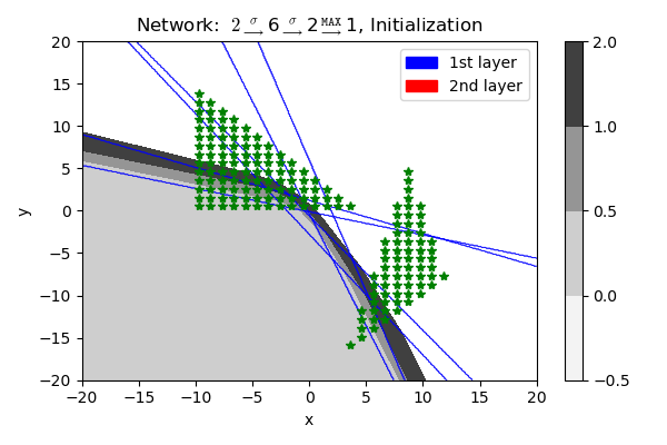
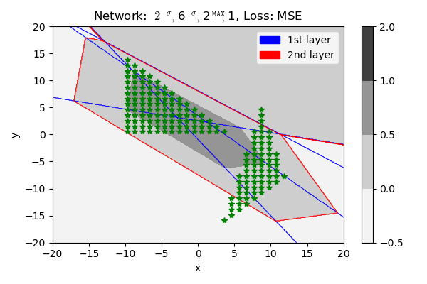
Refer to caption
Refer to caption
Refer to caption
Refer to caption
Refer to caption
Refer to caption
Refer to caption
Refer to caption
Refer to caption
Refer to caption
Refer to caption
Refer to caption
Refer to caption
Refer to caption
Refer to caption
Refer to caption
Refer to caption
Refer to caption
Refer to caption
Refer to caption
Refer to caption
Refer to caption
Refer to caption
Refer to caption
Refer to caption
Refer to caption
Refer to caption
Refer to caption
Refer to caption
Refer to caption
Refer to caption
Refer to caption
Figure 6: Initialization and convergence results to approximate 𝟙{𝒳2}subscript1subscript𝒳2\mathbbm{1}_{\{\mathcal{X}_{2}\}} via gradient descent. The first and third columns present the network initialization, and the second and fourth columns present the trained network under MSE and BCE loss, respectively. Each row has the same initialization scheme, which is given by uniform initialization U([0,1])𝑈01U([0,1]), normal initialization N(0,𝑰)𝑁0𝑰N(0,{\bm{I}}), Xavier uniform and normal initialization [9], He uniform and normal initialization [17], small-norm initialization, and manually initialized weights and bias, from top to bottom.
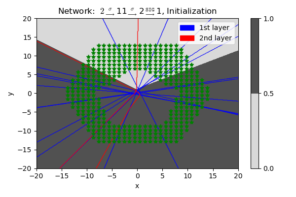
Refer to caption
Refer to caption
Refer to caption
Refer to caption
Refer to caption
Refer to caption
Refer to caption
Refer to caption
Refer to caption
Refer to caption
Refer to caption
Refer to caption
Refer to caption
Refer to caption
Refer to caption
Refer to caption
Refer to caption
Refer to caption
Refer to caption
Refer to caption
Refer to caption
Refer to caption
Refer to caption
Refer to caption
Refer to caption
Refer to caption
Refer to caption
Refer to caption
Refer to caption
Refer to caption
Refer to caption
Refer to caption
Figure 7: Initialization and convergence results to approximate 𝟙{𝒳2}subscript1subscript𝒳2\mathbbm{1}_{\{\mathcal{X}_{2}\}} via gradient descent. The first and third columns present the network initialization, and the second and fourth columns present the trained network under MSE and BCE loss, respectively. Each row has the same initialization scheme, which is given by uniform initialization U([0,1])𝑈01U([0,1]), normal initialization N(0,𝑰)𝑁0𝑰N(0,{\bm{I}}), Xavier uniform and normal initialization [9], He uniform and normal initialization [17], small-norm initialization, and manually initialized weights and bias, from top to bottom.