Neural incomplete factorization:
learning preconditioners for the conjugate gradient method

Abstract

Finding suitable preconditioners to accelerate iterative solution methods, such as the conjugate gradient method, is an active area of research. In this paper, we develop a computationally efficient data-driven approach to replace the typically hand-engineered algorithms with neural networks. Optimizing the condition number of the linear system directly is computationally infeasible. Instead, our method generates an incomplete factorization of the matrix and is, therefore, referred to as neural incomplete factorization (NeuralIF). For efficient training, we utilize a stochastic approximation of the Frobenius loss which only requires matrix-vector multiplications. At the core of our method is a novel message-passing block, inspired by sparse matrix theory, that aligns with the objective of finding a sparse factorization of the matrix. By replacing conventional preconditioners used within the conjugate gradient method by data-driven models based on graph neural networks, we accelerate the iterative solving procedure. We evaluate our proposed method on both a synthetic and a real-world problem arising from scientific computing and show its ability to reduce the solving time while remaining computationally efficient.

1 Introduction

Solving large-scale systems of linear equations is a fundamental problem in computing science. Available solving techniques can be divided into direct and iterative methods. While direct methods, which rely on computing the inverse or factorizing the matrix, obtain accurate solutions they do not scale well for large-scale problems. Therefore, iterative methods, which repeatedly refine an initial guess to approach the exact solution, are used in practice when an approximation of the solution is sufficient (Golub & Van Loan, 2013).

The conjugate gradient method is a classical iterative method for solving equation systems of the form ${\bm{A}}{\bm{x}}={\bm{b}}$ where the matrix ${\bm{A}}$ is symmetric and positive definite (Carson et al., 2023). Problems of this form arise naturally in the discretization of elliptical PDEs, such as the Poisson equation, and a wide range of optimization problems, such as quadratic programs (Pearson & Pestana, 2020; Potra & Wright, 2000). The convergence speed of the method thereby depends on the spectral properties of the matrix ${\bm{A}}$ (Golub & Van Loan, 2013). Therefore, it is common practice to improve the spectral properties of the equation system before solving it through the means of preconditioning. Despite the critical importance of preconditioners for practical performance, it has proven notoriously difficult to find good designs for a general class of problems (Saad, 2003).

Recent advances in data-driven optimization combine classical optimization algorithms with data-driven ones. A common approach is replacing hand-crafted heuristics with parameterized functions such as neural networks that are trained against data (Banert et al., 2021; Chen et al., 2022). In this work, we combine this methodology with results known from sparse matrix theory by representing the matrix of the linear equation system as a graph that forms the input to a graph neural network. We then train the network to predict a suitable preconditioner for the input matrix.

To train our model in a computationally feasible way we are inspired by the incomplete factorization methods. These methods, which include the popular incomplete Cholesky factorization, compute a sparse approximation of the Cholesky factor of the matrix ${\bm{A}}$ that is applied to precondition the linear system (Golub & Van Loan, 2013; Scott & Tůma, 2023). However, these methods can suffer from breakdown and require significant time to compute (Benzi, 2002). We overcome these limitations by introducing a scalable way to compute efficient preconditioners that do not suffer from breakdown. Our training scheme relies on matrix-vector multiplications only which can be implemented efficiently and allows us to train the method on large-scale problems. Further, we show how to control the obtained sparsity pattern of the learned preconditioner to obtain flexible preconditioning matrices (Saad, 2003).

In contrast to the NeuralPCG model introduced by Li et al. (2023), our model utilizes insights from graph theory to motivate the underlying computational framework and aligns with the training objective. This allows us to obtain more effective preconditioners using a smaller model which, in turn, leads to a faster inference time which is critical to amortize the cost of training and applying the neural network. Furthermore, our method is fully self-supervised while previous data-driven preconditioners rely on the solution of the linear equation system during training which increases the time required to generate a suitable dataset significantly.

2 Background

After introducing the conjugate gradient method, we briefly summarize basic graph neural networks which form the computational backend for our method.

2.1 Conjugate gradient method

The conjugate gradient method (CG) is a well-established iterative method for solving symmetric and positive-definite (spd denoted by $S^{++}_{n}$) systems of linear equations of the form ${\bm{A}}{\bm{x}}={\bm{b}}$. The algorithm does not require any matrix-matrix multiplications, making CG particularly effective when dealing with large and sparse matrices (Saad, 2003).

The method creates a sequence of search directions ${\bm{p}}_{i}$ which are orthogonal in ${\bm{A}}$-norm to each other i.e. ${\bm{p}}_{i}^{\mkern-1.5mu\mathsf{T}}{\bm{A}}{\bm{p}}_{j}=0$ for $i\neq j$. These search directions are used to update the solution iterate ${\bm{x}}_{k}$. Since it is possible to compute the optimal step size in closed form for each search direction, the method is guaranteed to converge within $n$ steps (Shewchuk, 1994). The iterative scheme is shown in Algorithm 1.

Convergence  The convergence of CG to the solution ${\bm{x}}_{\star}$ depends on the spectral properties of the matrix ${\bm{A}}$. Using the condition number $\kappa({\bm{A}})$, a linear bound of the error in the number of taken CG steps $k$ is given by (Carson et al., 2023)

$$\|{\bm{x}}_{\star}-{\bm{x}}_{k}\|_{\bm{A}}\leq 2\,\|{\bm{x}}_{\star}-{\bm{x}}_{0}\|_{\bm{A}}\left(\frac{\sqrt{\kappa({\bm{A}})}-1}{\sqrt{\kappa({\bm{A}})}+1}\right)^{k}\!.$$ (1)

However, in practice the CG method often converges significantly faster and the convergence also depends on the distribution of eigenvalues and the initial residual. Clustered eigenvalues hereby lead to faster convergence. Further, a large condition number needs not imply a slow convergence of the iterative scheme (Carson et al., 2023). A common approach to accelerate the convergence is to precondition the linear equation system to improve its spectral properties leading to faster convergence (Benzi, 2002).

Algorithm 1 Preconditioned conjugate gradient method (Nocedal & Wright, 1999)

1:  Input: System of linear equations ${\bm{A}}\in S_{n}^{++},{\bm{b}}\in\mathbb{R}^{n}$, Preconditioner ${\bm{P}}\approx{\bm{A}}$, ${\bm{P}}\in S_{n}^{++}$

2:  Output: Solution to the linear equation system $\hat{{\bm{x}}}_{\star}$

3:  Initialize starting guess ${\bm{x}}_{0}$

4:  ${\bm{r}}_{0}={\bm{b}}-{\bm{A}}{\bm{x}}_{0}$

5:  Solve ${\bm{P}}{\bm{y}}_{0}={\bm{r}}_{0}$ and set ${\bm{p}}_{0}={\bm{y}}_{0}$

6:  for $k=0,1,\ldots,$ until convergence do

7:     $a_{k}=\langle{\bm{r}}_{k},{\bm{y}}_{k}\rangle/\langle{\bm{A}}{\bm{p}}_{k},{\bm{p}}_{k}\rangle$

8:     ${\bm{x}}_{k+1}={\bm{x}}_{k}+a_{k}{\bm{p}}_{k}$

9:     ${\bm{r}}_{k+1}={\bm{r}}_{k}-a_{k}{\bm{A}}{\bm{p}}_{k}$

10:     Solve ${\bm{P}}{\bm{y}}_{k+1}={\bm{r}}_{k+1}$

11:     $\beta_{k}=\langle{\bm{r}}_{k+1},{\bm{y}}_{k+1}\rangle/\langle{\bm{r}}_{k},{\bm{y}}_{k}\rangle$

12:     ${\bm{p}}_{k+1}={\bm{y}}_{k+1}+\beta_{k}{\bm{p}}_{k}$

13:  end for

14:  return ${\bm{x}}_{k}$

Preconditioning  The underlying idea of preconditioning is to compute a cheap approximation of the inverse of ${\bm{A}}$ that is used to improve the convergence properties. A common way to achieve this is to approximate the matrix ${\bm{P}}\approx{\bm{A}}$ with an easily invertible preconditioning matrix ${\bm{P}}$. This can be achieved by constructing a (block) diagonal preconditioner or finding a (triangular) factorization (Benzi, 2002).

Finding a good preconditioner requires a trade-off between the time required to compute the preconditioner and the resulting speed-up in convergence (Golub & Van Loan, 2013). A simple way to construct a preconditioner called Jacobi preconditioner is to approximate ${\bm{A}}$ with a diagonal matrix. The incomplete Cholesky (IC) preconditioner is a more advanced method which is a widely adopted incomplete factorization method. As the name suggests, the idea is to approximate the Cholesky decomposition of the matrix. The IC(0) preconditioner restricts the non-zero elements in ${\bm{L}}$ to exactly the non-zero elements in the lower triangular part of ${\bm{A}}$. Thus, no fill-ins during the factorization are allowed. More general versions allow additional fill-ins of the matrix based on the position or the value of the matrix elements (Benzi, 2002; Scott & Tůma, 2023) or allow flexible positions of non-zero elements such as as the modified incomplete Cholesky (MIC) preconditioner (Lin & Moré, 1999).

Finding new preconditioners is an active research area but is often done on a case-by-case basis. Thus, newly developed methods are often tailor-made for specific problem classes and often do not generalize to new problem domains (Benzi, 2002; Pearson & Pestana, 2020).

Stopping criterion  In practice, due to numerical rounding errors, the residual is only approaching but never reaching zero. Further, the true solution ${\bm{x}}_{\star}$ is typically not available and therefore, equation (1) can not be used as a stopping criterion for the algorithm either. Instead, the relative residual error $\|{\bm{r}}\|_{2}$ which is computed recursively in line 9 of Algorithm 1 is widely adopted (Shewchuk, 1994).

2.2 Graph neural networks

A graph ${\mathcal{G}}=(V,E)$ is a tuple consisting of a set of nodes $V$ and directed edges $E$ connecting two nodes in the graph $E\subseteq V\times V$. We assign every node $v\in V$ a node feature vector ${\bm{x}}_{v}\in\mathbb{R}^{n}$ and respectively every directed edge $e_{ij}$, connecting nodes $i$ and $j$, an edge feature vector ${\bm{z}}_{ij}\in\mathbb{R}^{m}$.

Graph neural networks (GNN) belong to an emerging family of neural network architectures that are well-suited to many real-world problems which possess a natural graph structure (Veličković, 2023). The widely adopted message-passing GNNs consist of multiple layers updating the node and edge feature vectors of the graph iteratively using permutation invariant aggregations over the neighborhoods and learned update functions (Bronstein et al., 2021).

Here, we follow Battaglia et al. (2018) to describe the update functions for a simple message-passing GNN layer. In each layer $l$ the edge features are updated first by the network computing the features of the next layer $l+1$ as

$${\bm{z}}^{(l+1)}_{ij}=\phi_{{\bm{\theta}}^{(l)}_{z}}\left({\bm{z}}^{(l)}_{ij},{\bm{x}}^{(l)}_{i},{\bm{x}}^{(l)}_{j}\right),$$ (2)

where $\phi$ is a parameterized function. The outputs of this function are also referred to as messages. Then, for each node $i\in V$ the features from its neighboring edges, in other words, the messages, are aggregated using a suitable aggregation function. Typical choices include sum, mean and max aggregations. Any such permutation invariant aggregation function is denoted by $\oplus$. The aggregation of messages over the neighborhood $\mathcal{N}$ of node $n_{i}$ is computed as

$${\bm{m}}^{(l+1)}_{i}=\bigoplus_{j\in\mathcal{N}(i)}{\bm{z}}^{(l+1)}_{ji},$$ (3)

where this neighborhood is defined as $\mathcal{N}(i)=\{j\,|\,(i,j)\in E\}$. Note that the neighborhood structure is typically kept fixed in GNNs and no edges are added or removed between the different layers. The final step of the message-passing GNN layer is updating the node features as

$${\bm{x}}^{(l+1)}_{i}=\psi_{{\bm{\theta}}^{(l)}_{x}}\left({\bm{x}}^{(l)}_{i},{\bm{m}}_{i}^{(l+1)}\right).$$ (4)

The node and edge update functions $\phi$ and $\psi$ are parameterized using neural networks. The equations (2)–(4) describe the iterative scheme of message passing that is implemented by many popular GNNs. By choosing a permutation invariant function in the neighborhood aggregation step (3) and since the update functions only act locally on the node and edge features, the learned function represented by the GNN itself is permutation equivariant and can handle inputs of varying sizes (Battaglia et al., 2018).

Many known algorithms share a common computational structure with this scheme making GNNs a natural parameterization for learned variants. This is typically referred to as algorithmic alignment (Dudzik & Veličković, 2022).

3 Method

We formulate the learning problem for a data-driven preconditioner with an efficient loss function. Then, we introduce a problem-tailored GNN architecture, and demonstrate how to extend the framework to yield flexible sparsity patterns.

Learning problem  Our final goal is to learn a mapping $f_{{\bm{\theta}}}:S_{n}^{++}\to S_{n}^{++}$ that takes an spd matrix ${\bm{A}}$ and predicts a suitable preconditioner ${\bm{P}}$ that improves the spectral properties of the system – and therefore also the convergence behavior of the conjugate gradient method.

In order to ensure convergence, the output of the learned mapping needs to be spd and is in practice often required to be sparse due to resource constraints. To ensure these properties, we restrict the mapping to lower triangular matrices with strictly positive elements on the diagonal denoted as $\mathcal{L}_{n}^{+}$. We then learn a mapping $\Lambda_{{\bm{\theta}}}:\mathcal{S}_{n}^{++}\to\mathcal{L}_{n}^{+}$. This can be achieved by using a suitable activation function and network architecture as discussed later. The elements in $\mathcal{L}_{n}^{+}$ are guaranteed to be invertible and the computation thereof is computationally efficient since using forward-backward substitution requires only $\mathcal{O}(n^{2})$ operations (Golub & Van Loan, 2013). The parameterized function outputs a factorization of the preconditioning matrix that can be obtained via

$${\bm{P}}_{{\bm{\theta}}}({\bm{A}})=\Lambda_{{\bm{\theta}}}({\bm{A}})\Lambda_{{\bm{\theta}}}({\bm{A}})^{\mkern-1.5mu\mathsf{T}},$$ (5)

which is a spd matrix. To improve the convergence properties we aim to improve the condition number of the preconditioned system. However, computing the condition number scales very poorly for large problems as it requires $\mathcal{O}(n^{3})$ floating-point operations. Therefore, we can not optimize the spectral properties of the matrix directly. Instead, we are inspired by incomplete factorization methods (Benzi, 2002). These methods try to find a sparse approximation of the Cholesky factor of the input matrix while remaining computationally tractable. In order to learn a good approximation model we assume matrices of interest are generated by a matrix-valued random variable $\mathbb{A}$ with an unknown distribution describing the underlying class of problems.

We train our learned preconditioner to approximately solve the matrix factorization optimization problem with additional sparsity constraints given by

$$\hat{{\bm{\theta}}}\in\operatorname*{arg\,min}_{{\bm{\theta}}}\; \mathbb{E}_{{\bm{A}}\sim\mathbb{A}}\left[\|\Lambda_{{\bm{\theta}}}({\bm{A}})\Lambda_{{\bm{\theta}}}({\bm{A}})^{\mkern-1.5mu\mathsf{T}}-{\bm{A}}\|_{F}\right]$$ (6a)

s.t. $$\Lambda_{\bm{\theta}}({\bm{A}})_{ij}=0\text{ if }{\bm{A}}_{ij}=0.$$ (6b)

Equation (6a) aims to minimize the distance between the learned factorization and the input matrix using the Frobenius norm distance. It is, however, also possible to use a different distance metric instead (Vemulapalli & Jacobs, 2015).

When considering more advanced preconditioners, the no fill-in sparsity constraint (6b) can be relaxed slightly allowing more non-zero elements in the preconditioner. However, it is desirable that the required storage for the preconditioner is known beforehand and does not increase too much compared to the original system (Benzi, 2002).

A practical problem with objective (6a) is that we cannot compute the expectation since we lack access to the distribution of $\mathbb{A}$. On the other hand, we have access to training data ${\bm{A}}_{1},{\bm{A}}_{2},\ldots,{\bm{A}}_{n}\sim\mathbb{A}$, so we consider the empirical counterpart of equation (6) – empirical risk minimization – where the intractable expected value is replaced by the sample mean which we can optimize using stochastic gradient descent to obtain an approximation of $\hat{{\bm{\theta}}}$.

To enhance computational efficiency we circumvent computing the matrix-matrix multiplication $\Lambda_{{\bm{\theta}}}({\bm{A}})\Lambda_{{\bm{\theta}}}({\bm{A}})^{\mkern-1.5mu\mathsf{T}}$ in the objective, by approximating the Frobenius norm using Hutchinson’s trace estimator (Hutchinson, 1989) as

$$\|{\bm{B}}\|_{F}^{2}=\text{trace}({\bm{B}}^{\mkern-1.5mu\mathsf{T}}{\bm{B}})\approx\frac{1}{m}\sum_{i=1}^{m}{\bm{w}}_{i}^{\mkern-1.5mu\mathsf{T}}{\bm{B}}^{\mkern-1.5mu\mathsf{T}}{\bm{B}}{\bm{w}}_{i},$$ (7)

where ${\bm{w}}_{i}$ are iid normal distributed random variables. By setting ${\bm{B}}=\Lambda_{{\bm{\theta}}}({\bm{A}})\Lambda_{{\bm{\theta}}}({\bm{A}})^{\mkern-1.5mu\mathsf{T}}-{\bm{A}}$ and taking the square root of equation (7), we obtain an unbiased estimator of the loss which requires only matrix-vector products (Martinsson & Tropp, 2020). The resulting objective is similar to the loss proposed by Li et al. (2023) but does not rely on computing the true solution to the problem beforehand making it computationally more efficient as it avoids solving linear equation systems before the training. We show that using the approximation leads to similar results as training using the full Forbenius norm as a loss in Appendix C.2.

Model architecture  Due to the strong connection of graph neural networks with matrices and numerical linear algebra (Moore et al., 2023), it is a natural choice to parameterize the function $\Lambda_{\bm{\theta}}$ with a graph neural network. Furthermore, this allows us to enforce the sparsity constraints (6b) directly through the network architecture and avoids scalability issues arising in other network architectures since GNNs can exploit the sparse problem structure.

On a high level, we interpret the matrix ${\bm{A}}$ of the input problem as the adjacency matrix of the corresponding graph. Thus, the nodes of the graph represent the columns/rows – the system is symmetric – of the input matrix and are augmented with an additional feature vector. The edges of the corresponding graph are the non-zero elements in the adjacency matrix. This transformation from a matrix to a graph is known as Coates graph (Coates, 1959; Grementieri & Galeone, 2022). We use a total of eight node features related to sparsity structure and diagonal dominance of the matrix (Cai & Wang, 2019; Tang et al., 2022).

Since our learned function $\Lambda_{\theta}$ is mapping to a lower-triangular matrix, we implicitly fix an ordering of the nodes in the graph.

$$\begin{bmatrix}\mathbf{2.4}&{\color[rgb]{0,0,0}0.5}&{\color[rgb]{0,0,0}2.1}&0\\ {\color[rgb]{0,0.24609375,0.359375}0.5}&\mathbf{3.2}&{\color[rgb]{0,0,0}1.7}&0\\ {\color[rgb]{0.3984375,0.31640625,0.5703125}2.1}&{\color[rgb]{0.9765625,0.36328125,0.4140625}1.7}&\mathbf{7.5}&{\color[rgb]{0,0,0}2.0}\\ 0&0&{\color[rgb]{1,0.484375,0.26171875}2.0}&\mathbf{0.8}\\ \end{bmatrix}$$

Figure 1: Classical linear algebra and (lower triangular) graph representation of a spd matrix. Each node corresponds to the labeled row/column of the matrix. The upper triangular representation is obtained by flipping the edges. Color is used to visualize edge and matrix element correspondence. Diagonal elements are in bold.

To align our computational framework to the underlying objective of finding a sparse factorization, we introduce a novel GNN block that extends the Coates graph representation to execute the feature updates. Instead of using matrix ${\bm{A}}$ directly as the underlying structure for message passing, we only use the lower triangular part in the first step to update node and edge features in the graph. This lower triangular structure also aligns with sparsity pattern of the final output $\Lambda_{\bm{\theta}}$. The corresponding graph used for message passing is depicted in Figure 1.

In a second step, the message-passing scheme is executed over the upper triangular part of the matrix ${\bm{A}}$. However, the edge features between the two consecutive layers are shared i.e. ${\bm{z}}_{ij}^{(n)}={\bm{z}}_{ji}^{(n)}$. After the two message-passing steps, the original matrix ${\bm{A}}$ is used to augment the edge features by introducing skip connections. The block implementation shares node features across the layer, resulting in an equivalent Coates graph representation with two distinct set of edges ${\bm{L}}$ and ${\bm{L}}^{\mkern-1.5mu\mathsf{T}}$. For each set of edges, an individual message-passing step is performed which consists of the node update, neighborhood aggregation, and edge update as described in Section 2.2. The detailed forward pass through the network architecture is described in Appendix B.

The underlying motivation of the message-passing block is the fact that matrix multiplication can be represented in graph format by concatenating the graph representations of the two factors. Each element in the product matrix can then be computed as the sum of the weights connecting the two corresponding nodes in the concatenated graphs. The skip connections are introduced as they represent an element-wise addition of the two matrices (Doob, 1984; Brualdi & Cvetkovic, 2008). Furthermore, the proposed splitting into lower and upper parts directly encodes the ordering used to obtain the triangular output into the network structure.

Our model consists of $N=3$ of these blocks resulting in a total of six message-passing steps. To enforce the positive definiteness of the learned preconditioner the final diagonal elements of the output are transformed via

$$\Lambda_{\bm{\theta}}({\bm{A}})_{ii}=\sqrt{\exp\left({z}_{ii}^{(N)}\right)}.$$ (8)

This activation function forces the diagonal elements to be strictly positive. Taking the square root avoids numerical problems and, based on our experiments, has demonstrated improved convergence during training. In total, this leads to a model consisting of $1\thinspace 780$ parameters. Due to the connection to incomplete factorization methods, we refer to our model as neural incomplete factorization (NeuralIF).

Additional fill-ins and droppings  Similar to the incomplete Cholesky method with additional fill-ins (Saad, 2003), processing on the graph can be applied to obtain both static and dynamic sparsity patterns for the learned preconditioner. Static level of fill-ins can be obtained by adding additional edges to the graph prior to the message passing during the symbolic phase. This corresponds to relaxing constraint (6b) to allow more non-zero elements for example by allowing all entries corresponding to the sparsity pattern of ${\bm{A}}^{2}$.

To obtain a dynamic sparsity pattern, we add a $\ell_{1}$-penalty on the elements in the learned preconditioning matrix $\|\Lambda_{\bm{\theta}}({\bm{A}})\|_{1}$ to the training objective (6a). This encourages the network to produce sparse outputs (Jenatton et al., 2011). During inference, we drop elements with a small magnitude to obtain an even sparse preconditioner. This can lead to faster overall solving times since the step to find the search direction in line 9 of Algorithm 1 scales with the number of non-zero elements in the preconditioner (Davis et al., 2016). Both of these approaches can also be combined to obtain a learned preconditioner similar to the dual threshold incomplete factorization (Saad, 1994).

By including additional edges, the forward pass of the GNN becomes computationally more expensive. Therefore, it is important to avoid increasing the non-zero elements too much to maintain the computational efficiency. Dropping additional elements, on the other hand, can be achieved with nearly no overhead during inference.

Inference and amortization  When the trained model is used during inference time to generate preconditioners, the output ${\bm{P}}_{\theta}({\bm{A}})=\Lambda_{\theta}({\bm{A}})\Lambda_{\theta}({\bm{A}})^{\mkern-1.5mu\mathsf{T}}\approx{\bm{A}}$ is used within Algorithm 1 to find the preconditioned search direction. The implementation details can be found in Appendix B.

4 Results

The overall goal is to reduce total computational time required to solve the problem up to a given precision (here, we choose $10^{-6}$) measured by the residual norm as described in Section 3. The time used to compute the preconditioner beforehand, therefore, needs to be traded off with the achieved speed-up through the usage of the preconditioner. We compare the different methods based on both the time required to compute the preconditioner (P-time) and the time needed to solve the preconditioned linear equation system (CG-time) which is related to the number of iterations required.

We consider two different datasets. The first dataset consists of synthetically generated problems where we can easily control the size and the generated sparsity. The other problem arises from scientific computing by discretizing the Poisson PDE on varying grids using the finite element method. The details for the dataset generation can be found in Appendix A and implementation details of the different baselines and methods are described in Appendix B.

Further acceleration of our neural network-based preconditioner can be obtained by batching the problem instances. This allows parallelization of the computation for the preconditioners leading to a smaller precomputation overhead. However, to ensure a fair comparison in our experiments, we handle each problem individually.

4.1 Synthetic problems

The results and statistics about the preconditioned systems from the experiments using the synthetic dataset are shown in Table 1. We can see that the learned preconditioner is significantly faster to compute while maintaining similar performance in terms of reduction in number of iterations as the incomplete Cholesky method. This makes our approach on average $\sim 25\%$ faster than incomplete Cholesky. Compared to NeuralPCG, our method is faster to compute, since the number of parameters is significantly smaller. Further, we are able to reduce the number of required iterations to solve the problem more.

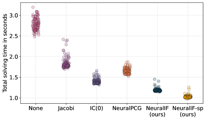
Figure 2: Total solving time for each test problem instance from the synthetic dataset.

Table 1: Mean results for the synthetic dataset for $n=10\thinspace 000$ on $100$ test instances. The first column shows the condition number of the preconditioned system ${\bm{L}}^{-1}{\bm{A}}{\bm{L}}^{-{\mkern-1.5mu\mathsf{T}}}$. The second column lists the preconditioner’s sparsity. Remaining columns list performance-related figures for the preconditioned conjugate gradient method: the third column lists the computation time for the preconditioner (P-time), the fourth lists the time for finding the solution and the number of iterations required running the preconditioned conjugate gradient method (CG-time/Iters.) and the fifth column shows the combined time for computing the preconditioner and solving the system. All times are in seconds. The final column shows the percentage of successfully solved instances. Arrows indicate whether higher/lower is better.

Preconditioner	Condition number $\kappa\downarrow$	Sparsity $\uparrow$	P-time $\downarrow$	CG-time (Iters.) $\downarrow$	Total time $\downarrow$	Success $\uparrow$
None	60 834.17	-	-	2.79 (935.99)	2.79	100%
Jacobi	33 428.86	99.99%	0.005	1.83 (689.82)	1.84	100%
IC(0)	4 707.17	99.49%	0.247	1.16 (260.64)	1.40	96%
NeuralPCG	7 240.72	99.49%	0.123	1.54 (318.86)	1.66	100%
NeuralIF (ours)	4 921.76	99.49%	0.028	1.16 (267.08)	1.19	100%
NeuralIF-sp (ours)	5 581.44	99.77%	0.021	1.01 (286.02)	1.03	100%

The distribution of total solving times is shown in Figure 2, where each point represents a single test problem instance that is solved. Overall, the variance of solving time between different problems is small for all considered methods. Further, we can see that both of our NeuralIF preconditioners outperforms the other preconditioning methods on nearly all problem instances.

Dynamic sparsity pattern  The results for the learned preconditioner with additional sparsity, through dropping elements by value, are shown as NeuralIF-sp. Even though the output of the model contains only around half of the elements compared to the methods without fill-ins, the performance in terms of iterations does not suffer significantly. Therefore, the overall time to solve the system is on average shortest using the sparsified NeuralIF preconditioner across all tested preconditioning methods.

Eigenvalue distribution  In Figure 3, the ordered eigenvalues of the preconditioned linear equation system for one test problem are shown. Here, we can see that NeuralIF is especially able to reduce large eigenvalues compared to the other preconditioners. However, compared to incomplete Cholesky the smaller eigenvalues of the NeuralIF preconditioned system decrease earlier and the smallest eigenvalue of the system is slightly smaller.

Breakdown  The incomplete Cholesky method suffers from breakdown in some of the test problems

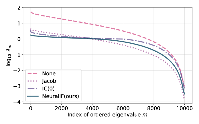
Figure 3: Ordered eigenvalues of the preconditioned linear equation system in log-scale for one synthetic problem instance.

due to the inherent numerical instabilities of the method (Benzi, 2002). These instances are not included in solving time in Table 1 but are very costly in practice since it requires a restart of the solving procedure. In contrast, our data-driven approach consistently generates a suitable preconditioner.

4.2 Poisson PDE problems

In the second problem, we are focusing on problems arising from the discretization of Poisson PDEs. In order to train our learned preconditioner efficiently, we create a subset of small training problems with matrices of size between 20 000 and 100 000 with up to 500 000 non-zero elements. The results for these problems are summarized in Table 2. Here, MIC is the modified incomplete Cholesky method with the same number of non-zero elements as IC(0) but potentially different locations of the non-zero elements (Lin & Moré, 1999). Among all preconditioners without fill-ins, our method performs best as it is very efficient to compute and reduces the required iterations vastly.

The MIC+ preconditioner further allows additional fill-ins based on the number of non-zero elements in each row of the matrix which improves the preconditioner at the cost of a more expensive pre-computation time. Our NeuralIF(1) preconditioner is obtained by allowing non-zero elements in the non-zero locations of the matrix ${\bm{A}}^{2}$. Here, computing the static sparsity pattern before the message passing requires a significant amount of time. Therefore, the highly optimized implementation of the modified incomplete Cholesky method performs slightly better but the learned preconditioner improves significantly due to the added fill-ins compare to the previous methods without fill-ins.

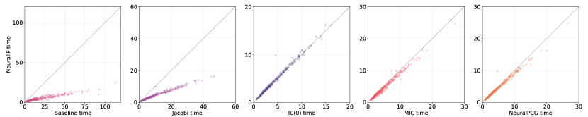
Figure 4: Pairwise comparison of NeuralIF with the other preconditioners without fill-ins on the 300 large PDE problem instances. Instances in the lower right part of the plot indicate that our method is faster, otherwise the baseline. Note that there are different axis scales for each comparison.

Since real-world problems are often significantly larger than the training instances, we evaluate our methods also on problem instances of sizes up to 500 000 containing $3\thinspace 000\thinspace 000$ non-zero elements. Since the problems in the dataset containing large instances are more diverse in terms of size, number of non-zero elements, and difficulty in solving them compared to the training dataset, we show a pairwise comparison in Figure 4. Here, we compare the time it takes to solve the system using NeuralIF to solving the problem using various other preconditioners. We can see that for the larger problem instances, the NeuralIF preconditioner performs on par with the IC(0) method and even outperforms MIC, even though the problems are significantly larger than the training instances showing the good generalization abilities of our method.

Table 2: Results for the small Poisson PDE problems from the training distribution using a subset of the columns shown in Table 1. The first set of method does not use fill-ins while in the second part additional non-zeros are added.

Preconditioner	P-time	CG-time (Its.)	Total time
None	-	1.72 (856.38)	1.72
Jacobi	0.004	1.01 (466.85)	1.02
IC(0)	0.022	0.51 (166.05)	0.53
MIC	0.029	0.56 (180.94)	0.59
NeuralPCG	0.018	0.57 (189.97)	0.59
NeuralIF(0)	0.014	0.51 (168.09)	0.52
MIC+	0.044	0.39 (100.95)	0.43
NeuralIF(1)	0.030	0.44 (111.37)	0.47

Additional results on preconditioning and scalability can be found in Appendix C.

5 Discussion & Limitations

To train data-driven preconditioners, we assume that there is a sufficiently large set of problem instances that share some similarity and need to be solved efficiently in the form of a distribution $\mathbb{A}$. In practice, finding such a distribution is challenging for some problem domains. Further, the time invested in the model training needs to be amortized over the speedup obtained during the inference phase of the learned preconditioner. However, this model training replaces the otherwise time-consuming manual tuning of preconditioners and is not a specific issue with our method but a limitation of the general learning-to-optimize framework (Chen et al., 2022). This also motivates following our self-supervised learning approach since it allows us to train the model on unsolved problem instances. The trained model can then, in principle, be applied to accelerate solving the training instances making it easier to amortize the model training.

While the method works well in our numerical experiments, no guarantees about the convergence speed can be made and it is likely that for some problem classes the usage of the learned preconditioner leads to an increase in overall solving time. That said, as seen in the experiments also classical preconditioners suffer from this problem and our method avoids pitfalls such as breakdowns in incomplete Cholesky.

A promising future research direction is to learn the sparsity pattern used for the preconditioner alongside the values to fill in. This can be achieved by changing the graph structure used for message passing but requires additional care due to the combinatorial nature of the problem. Further, the incomplete factorization loss used to train our model is only a heuristic and not directly related to the complex convergence behavior of the conjugate gradient method. Extending the approach to directly take into account the downstream task has the potential to further improve the learned preconditioner and lead to faster convergence (Bansal et al., 2023).

6 Related work

Data-driven optimization or “learning-to-optimize (L2O)” is an emerging field aiming to accelerate numerical optimization methods by combining them with data-driven techniques (Amos, 2023). For example, a neural network can be trained to directly predict the solution to an optimization problem (Grementieri & Galeone, 2022) or replace some hand-crafted heuristic within a known optimization algorithm (Bengio et al., 2021).

L2O using GNNs  Graph neural networks have been recognized as a suitable computational backend for problems in data-driven optimization (Moore et al., 2023). Chen et al. (2023) study the expressiveness of GNNs with respect to their power to represent linear programs on a theoretical level. Using the Coates graph representation, Grementieri & Galeone (2022) develop a sparse linear solver for linear equation systems. They represent the linear equation system as the input to a graph neural network which is trained to approximate the solution to the equation system directly. However, no guarantees for the solution can be obtained. In contrast, our method benefits from the convergence properties of the preconditioned conjugate gradient method.

Following an AutoML approach, Tang et al. (2022) instead try to predict a good combination of solver and preconditioner from a predefined list of techniques using supervised training. The NeuralIF preconditioner instead focuses on further accelerating the existing CG method and does not need any explicit supervision during training. Sjölund & Bånkestad (2022) use the König graph representation instead to accelerate low-rank matrix factorization algorithms by representing the matrix multiplication as a concatenation graph similar to our approach. However, their architecture utilizes a graph transformer while our approach works in a fully sparse setting. This avoids the scalability issues of transformer architectures and makes it better suited for large-scale problems.

Data-driven CG  Incorporating deep learning into the conjugate gradient method has been utilized in several ways previously. Kaneda et al. (2023) suggest replacing the search direction in the conjugate gradient method with the output of a neural network. This approach can, however, not be integrated with existing solutions for accelerating the CG method and does not allow further improvements through preconditioning. Furthermore, to ensure convergence all previous search directions need to be saved and the full Gram–Schmidt orthonormalization needs to be computed in every iteration making it prohibitively expensive.

There have also been some earlier approaches to learning preconditioners for the conjugate gradient method following similar ideas as our proposed NeuralIF method. Ackmann et al. (2021) use a fully-connected neural network to predict the preconditioner for climate modeling using a supervised loss. Sappl et al. (2019) use a convolutional neural network (CNN) to learn a preconditioner for applications in water engineering by optimizing the condition number directly. However, both of these approaches are only able to handle small-scale problems and their architecture and training is limited due to their poor scalability compared to our suggested approach. Utilizing CNN architectures, predicting sparsity patterns for specific types of preconditioners (Götz & Anzt, 2018) and general incomplete factorizations (Stanaityte, 2020) has also been suggested. In comparison, our learned method is far more general and can be applied to a significantly larger class of problems.

Preconditioning  Incomplete factorization methods are a large area of research. In most cases, the aim is to reduce computational time and memory requirements by ignoring elements based on either position or value. However, if done too aggressively, the method may break down due to numerical issues and require expensive restarts. Perturbation and pivoting techniques can mitigate but not completely eliminate such problems (Scott & Tůma, 2023). In contrast, our method does not suffer from breakdown as the positive-definiteness of the output is ensured a posteriori. Numerical efficiency can also be improved by reordering to reduce fill-in (for IC($\ell$) with $\ell>0$) or by finding rows of the matrix that can be eliminated in parallel (Gonzaga de Oliveira et al., 2018). Chow & Patel (2015) formulate incomplete factorization as the problem of finding a factorization that is exact on the given sparsity pattern as a feasibility problem that can be solved approximately. In contrast, our method only approximates the Frobenius norm minimization in equation (6) without enforcing constraints, which reduces pre-computation times.

For problems arising from elliptical PDEs, multigrid preconditioning techniques have shown to be very effective. These type of methods utilize the underlying geometric structure of the problem to obtain a preconditioner (Pearson & Pestana, 2020). Multigrid methods have also been successfully combined with deep learning techniques (Azulay & Treister, 2022). A potential drawback of this type of preconditioner is, however, that the technique is computationally quite expensive compared to other methods and the resulting preconditioner is typically non-sparse.

7 Conclusions

In this paper we introduce NeuralIF, a novel and computationally efficient data-driven preconditioner for the conjugate gradient method to accelerate solving large-scale linear equation systems. Our method is trained to predict the sparse Cholesky factor of the input matrix following the widespread idea of incomplete factorization preconditioners (Benzi, 2002). We use the problem matrix as an input to a graph neural network. The network architecture aligns with the objective to minimize the distance between the learned output and the input using a the Frobenius norm as a distance measure using insights from graph theory. Our experiments show that the proposed method is competitive against general-purpose preconditioners both on synthetic and real-world problems and allows the creation of both dynamic and static sparsity patterns. Our work shows the large potential of data-driven techniques in combination with insights from numerical optimization and the usefulness of graph neural networks as a natural computational backend for problems arising in computational linear algebra (Moore et al., 2023).

Appendix A Dataset details

The (preconditioned) conjugate gradient method is a standard iterative method for solving large-scale systems of linear equations of the form

$${\bm{A}}{\bm{x}}={\bm{b}}$$ (9)

where ${\bm{A}}$ is symmetric and positive definite (spd) i.e. ${\bm{A}}={\bm{A}}^{\mkern-1.5mu\mathsf{T}}$ and ${\bm{x}}^{\mkern-1.5mu\mathsf{T}}{\bm{A}}{\bm{x}}>0$ for all ${\bm{x}}\neq 0$. We also write ${\bm{A}}\in S_{n}^{++}$ to indicate that ${\bm{A}}$ is a $n\times n$ spd matrix (Golub & Van Loan, 2013). The method is especially efficient when the matrix ${\bm{A}}$ is large-scale and sparse since the required matrix-vector products shown in Algorithm 1 can efficiently exploit the structure of the matrix in this case (Saad, 2003).

In this section, we specify different problem settings leading to distributions $\mathbb{A}$ over matrices of the desired form such that the conjugate gradient method is a natural choice for solving the problem. Given a distribution we accessing via a number of samples, our goal is to train a model using the empirical risk minimization objective shown in the main paper to compute an incomplete factorization of a given input and utilize the resulting output as an effective preconditioner in the CG algorithm.

In total, we are testing our method on two different datasets but vary the parameters used to generate these datasets. The first problem dataset considers synthetic problem instances. The other test problem arises in scientific computing where large-scale spd linear equation systems can be obtained naturally from the discretization of elliptical PDEs. In Section C, the results presented in the main paper on these problem settings are extended.

The size of the matrices considered in the experiments is between $n=10\thinspace 000$ and $n=200\thinspace 000$ for all datasets in use. Throughout the paper we assume that the problem at hand is (very) sparse and spd. Thus, the preconditioned conjugate gradient method is a natural choice for all these problems. We ensure that the matrices are different by using unique and non-overlapping seeds for the problem generation. The datasets are summarized in Table 3. For the graph representation used in the learned preconditioner, the matrix size corresponds to the number of nodes in the graph and the number of non-zero elements corresponds to the number of edges connecting the nodes. In the following, the details for the problem generation are explained for each of the datasets.

Table 3: Summary of the datasets used with some additional statistics on size of the matrices and the number of corresponding non-zero elements. Samples refer to number of generated problems in the train, validation and test set respectively.

Dataset	Samples	Matrix size	Non-zero elements	Sparsity
Synthetic	1 000/10/100	10 000	$\sim 1\thinspace 000\thinspace 000$	$99\%$
Poisson PDE - train	750/15/300	20 000 – 150 000	800 000 – 500 000	$>99.9\%$
Poisson PDE - test	-/-/300	100 000 – 500 000	500 000 – 3 000 000	$>99.9\%$

A.1 Synthetic problem

The set of random test matrices is constructed by choosing a sparsity parameter $p$ which indicates the expected percentage of non-zero elements in the matrix. It is also possible to specify $p$ itself as a distribution. We choose the non-zero probability such that the resulting spd matrices which are generated with equation equation (10) have around $99\%$ total sparsity (therefore the generated problems have 1 million non-zero elements). For the out-of-distribution data, we sample the sparsity probability uniform such that the resulting matrices have between 50 000 and 5 000 000 non-zero elements. We then create the problem by sampling a matrix ${\bm{A}}$ with $p({\bm{A}}_{ij}=0)=p$ and $p({\bm{A}}_{ij}|{\bm{A}}_{ij}\neq 0)\sim\mathcal{N}(0,1)$. The final problem is then given by

$${\bm{M}}={\bm{A}}{\bm{A}}^{\mkern-1.5mu\mathsf{T}}+\alpha{\bm{I}}$$ (10)

where $\alpha\approx 10^{-3}$ is used to ensure the resulting problem is positive definite. The right hand side of the linear equation system is sampled uniformly ${\bm{b}}\sim\mathcal{U}[0,1]^{n}$.

Problems of this form also arise when minimizing quadratic programs since the equation equation (9) represents the first-order optimality condition for an unconstrained QP (Stellato et al., 2020). Thus, the problem represented here can be encountered in various settings making it an interesting case study.

A.2 Poisson equation

The Poisson equation is an elliptical partial differential equation (PDE) and one of the most fundamental problems in numerical computational science (Langtangen & Logg, 2016). The problem is stated as solving the boundary value problem

$$-\nabla^{2}u(x) =f(x)\;\;\;\;\;\;x\in\Omega$$ (11a)

$$u(x) =u_{D}(x)\;\;\;\,x\in\partial\,\Omega$$ (11b)

where $f(x)$ is the source function and $u=u(x)$ is the unknown function to be solved for. By discretizing this problem using the finite element method and writing it in matrix form a system of linear equations of the form ${\bm{L}}{\bm{x}}={\bm{b}}$ is obtained where the stiffness matrix ${\bm{L}}$ is sparse and spd. For large $n$, this problem therefore can be efficiently solved using the conjugate gradient method given a good preconditioner.

In order to obtain a distribution $\mathbb{A}$ over a large number of Poisson equation PDE problems, we consider a set of meshes that are generated by sampling from a normal distribution and creating a mesh based on the sampled points. We consider three different cases for the mesh generation: (a) we form the convex hull of the sampled points and triangulate the resulting shape, (b) we sample two sets of points and transform them into convex shapes as before. The second samples have a significantly smaller variance. The final shape that is used for triangulation is then obtained as the difference between the two samples. Finally, (c) we generate a simple polytope from the sampled points. An example for each of the generated shapes is shown in Figure 5. The sampled meshes are discretized using the finite-element method and refined using the scikit-fem python library (Gustafsson & McBain, 2020). Due to the discretization based on the provided mesh the size of the generated matrix is variable. Based on the stiffness matrices arising from the discretized problems the NeuralIF preconditioner is trained.

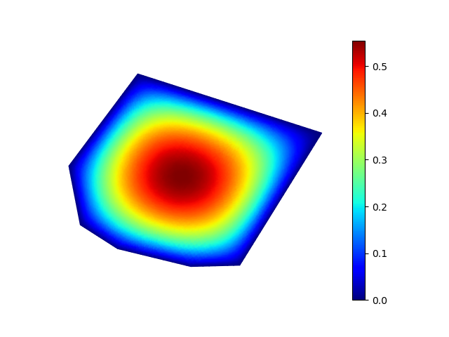
(a) Convex

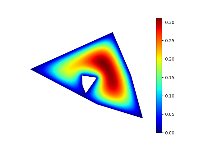
(b) Convex with hole

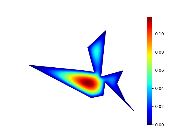
(c) Simple polytope

Figure 5: Sample meshes for each of the three different domain distributions used to generate training data for the Poisson PDE problem.

Appendix B Implementation details

In the following, we describe the details of the network architecture our NeuralIF model uses as well as the details of the model training, testing, and inference. Our method is implemented using PyTorch (Paszke et al., 2019) and PyTorch Geometric (Fey & Lenssen, 2019).

B.1 NeuralIF architecture

Node and edge features  In total eight features are used for each node thus ${\bm{x}}_{i}\in\mathbb{R}^{8}$. The first five node features listed in Table 4 are implemented following the local degree profile introduced by Cai & Wang (2019). The dominance and decay features shown in the table are originally introduced by Tang et al. (2022).

As edge feature, only the scalar value of the matrix entry is used. In deeper layers of the network, when skip connections are introduced, the edges are augmented with the original matrix entries. This effectively leads to having two edge features in these layers: the computed edge embedding of the current layer ${\bm{z}}_{ij}^{(l)}$ as well as the original matrix entry $a_{ij}$. However, from these only a one-dimensional output is computed ${\bm{z}}_{ij}^{(l+1)}$ as described in the following.

Table 4: List of node features used in the graph neural network.

Feature name	Description
deg(v)	Degree of node $v$
max deg(u)	Maximum degree of neighboring nodes
min deg(u)	Minimum degree of neighboring nodes
mean deg(u)	Average degree of neighboring nodes
var deg(u)	Variance in the degrees of neighboring nodes
dominance	Diagonal dominance
decay	Diagonal decaying
pos	The position of the node in the matrix

Message passing block  At the core of our method, we introduce a novel message passing block which aligns with the objective of our training. The underlying idea is that matrix multiplication can be represented in graph form by concatenating the two Coates graph representations as described previously (Doob, 1984). The pseudocode for the message passing scheme is shown in Algorithm 2. The message passing block consists of two GNN layers as introduced in Section 3 which are concatenated to mimic the matrix multiplication. To align the block with our objective, we only consider the edges in the lower triangular part of the matrix in the first layer (see lines 8–11 in Algorithm 2) while in the second layer of the block only edges from the upper triangular part of the matrix are used (lines 14–17). However, the same edge embedding for the two steps are used (line 13). In the final step of the message passing block, we introduce skip connections and concatenate the edge features in the current layer with the original matrix entries (lines 18–23). Note that, since the matrix ${\bm{A}}$ is symmetric it holds that $(i,j)\in L\Leftrightarrow(j,i)\in U$ where $U$ and $L$ are the index set corresponding to the non-zero elements in the upper and lower triangular matrix.

Here, we denote the updates after the first message passing layer with the superscript $(l+\frac{1}{2})$ to explicitly indicate that it is an intermediate update step. The final output from the block is then computed based on another message passing step which utilizes the computed intermediate embedding. Further, $\mathcal{N}_{L}(i)$ denotes the neighborhood of node $i$ with respect to the edges in the lower triangular part ${\bm{L}}$ and $\mathcal{N}_{U}(i)$ the ones from the upper triangular part ${\bm{U}}$ respectively which are utilized for the message passing. There are always at least the diagonal elements in the neighborhood of each node and therefore, the message computation is well defined.

Network design  Both the parameterized edge update $\phi$ and the node update $\psi$ functions in every layer are implemented using two layer fully-connected neural networks. The inputs to the edge update network $\phi$ are formed by the node features of the corresponding edge and the edge features themselves leading to a total of $8+8+1=17$ inputs in the first message passing step and one additional input in later steps. The edge network outputs a scalar value. For each network, eight hidden units are used and the tanh activation function is applied as a non-linearity. To compute the aggregation over the neighborhood $\oplus$, the mean and sum aggregation functions are used – respectively in the first and second step of the message passing block – which is applied component-wise to the set of neighborhood edge feature vectors. The node update function $\psi$ takes the aggregation of the incoming edge features as well as the current node feature as an input ($1+8=9)$.

The NeuralIF model used in the experiments consists of $3$ of the message passing blocks introduced in Section 3. Resulting in a total of six GNN message passing steps with two skip connections from the input matrix $A$. Graph normalization prior to the message passing leads to faster overall convergence of the training process (Cai et al., 2021). Note, that the graph normalization step is independent of the graph topology and only operates on the node feature vectors. In total the NeuralIF GNN model has $1\thinspace 870$ learnable parameters. The forward pass through the model is described in Algorithm 2.

Training  We are training our model for a total of $50$ epochs using a batch size of $5$ for the synthetic problems and $1$ for PDE problems. The Adam optimizer with initial learning rate $0.001$ is used. Due to the small batch size and the loss landscape, we utilize gradient clipping to restrict the length of the allowed update steps and reduce the variance during stochastic gradient descent. While we use the Hutchinson’s trace estimator with $m=1$ during training which allows a full vectorized implementation of the problem loss function. We compute the full Frobenius norm during the validation phase to avoid overfitting and ensure convergence. We use early stopping in order to avoid overfitting of the model based on the validation set performance by using the number of iterations the learned preconditioner takes on the validation data as the target.

Algorithm 2 Pseudo-code for NeuralIF preconditioner.

1:  Input: Graph representation of the spd system of linear equations ${\bm{A}}{\bm{x}}={\bm{b}}$.

2:  Output: Lower-triangular sparse preconditioner for the linear system which is an incomplete factorization.

3:  $\triangleright$ NeuralIF preconditioner computation:

4:  Compute node features ${\bm{x}}_{i}$ shown in Table 4

5:  Apply graph normalization

6:  Split graph adjacency matrix into index set for the lower and upper triangular parts, $L$ and $U$.

7:  for each message passing block $l$ in $0,1,\ldots,N-1$ do

8:     $\triangleright$ update using the lower-triangular matrix part

9:     $z_{ij}^{(l+\frac{1}{2})}\leftarrow\phi_{{\bm{\theta}}_{z,1}^{{l}}}({\bm{z}}_{ij}^{(l)},{\bm{x}}_{i}^{(l)},{\bm{x}}_{j}^{(l)})$ for all $(i,j)\in L$

10:     $m_{i}^{(l+\frac{1}{2})}\leftarrow\bigoplus^{(1)}_{j\in\mathcal{N}_{L}(i)}z_{ji}^{(l+\frac{1}{2})}$

11:     ${\bm{x}}_{i}^{(l+\frac{1}{2})}\leftarrow\psi_{{\bm{\theta}}_{e,1}^{{l}}}({\bm{x}}_{i}^{(l)},m_{i}^{(l+\frac{1}{2})})$

12:     $\triangleright$ share the computed edge updates between the layers

13:     $z_{ji}^{(l+\frac{1}{2})}\leftarrow z_{ij}^{(l+\frac{1}{2})}$ for all $(i,j)\in L$

14:     $\triangleright$ update using the upper triangular matrix part

15:     $z_{ji}^{(l+1)}\leftarrow\phi_{\theta_{z,2}^{{l}}}(z_{ji}^{(l+\frac{1}{2})},x_{j}^{(l+\frac{1}{2})},x_{i}^{(l+\frac{1}{2})})$ for all $(j,i)\in U$

16:     $m_{i}^{(l+1)}\leftarrow\bigoplus^{(2)}_{j\in\mathcal{N}_{U}(i)}z_{ji}^{(l+1)}$

17:     $x_{i}^{(l+1)}\leftarrow\psi_{\theta_{e,2}^{{l}}}(x_{i}^{(l)},m_{i}^{(l+1)})$

18:     if not final layer in the network then

19:        $\triangleright$ add skip connections

20:        $z_{ij}^{(l+1)}\leftarrow[z_{ji}^{(l+1)},a_{ji}]^{\mkern-1.5mu\mathsf{T}}$ for all $(j,i)\in U$

21:     else

22:        $z_{ij}^{(l+1)}\leftarrow z_{ji}^{(l+1)}$ for all $(j,i)\in U$

23:     end if

24:  end for

25:  Apply $\sqrt{\exp(\cdot)}$-activation function to final edge embedding of diagonal matrix entries $z_{ii}^{(N)}$.

26:  Return lower triangular matrix with elements $z_{ij}^{(N)}$ for $i\leq j$.

B.2 Baselines

Conjugate gradient method  The conjugate gradient method is implemented both in the preconditioned form (as shown in Algorithm 1) and, as a baseline, without preconditioner using PyTorch only relying on matrix-vector products which can be computed efficiently in sparse format (Paszke et al., 2019). In order to ensure an efficient utilization of the computed preconditioners, the forward-backward substitution to solve for the search direction is implemented using the triangular solve method provided in the numml package for sparse linear algebra (Nytko et al., 2022). The conjugate gradient method is run until the normalized residual reaches a threshold of $10^{-6}$, see Section 3 for details.

Compute  To avoid overhead due to the initialization of the CUDA environment, we run a model warm-up with a dummy input, before running inference tests with our model. The (preconditioned) conjugate gradient method – including the sparse forward-backward triangular solves for the utilized preconditioner – is run on a single-thread CPU.

Preconditioner  The Jacobi is due to its computationally simplicity, directly implemented in PyTorch and scipy using a fully vectorized implementation. It can be seen in the numerical experiments that the overhead for computing this method is very small compared to the more advanced preconditioners. The incomplete Cholesky preconditioners and its modified variants with dynamic sparsity patterns and additional fill-ins are implemented using the highly efficient C++ implementation of ILU++ with provided bindings to python (Mayer, 2007; Hofreither, 2020).

The data-driven NeuralPCG baseline – which uses a simple encoder-decoder GNN architecture – (Li et al., 2023) is implemented in pyTorch and pyTorch geometric following a very similar approach to NeuralIF. The hyper-parameters for the model are chosen as specified in the paper: using $16$ hidden units with a single hidden layer for encoder, decoder and GNN update functions and a total of $5$ message passing steps. This results in a total of $10\thinspace 177$ parameters in the model which means the parameter count is over 5 times higher than our proposed architecture which makes inference using the NeuralPCG model more expensive during inference. Due to computational limits, the batch size is reduced during training compared to the original paper.

The results obtained from the model are similar to the one presented by Li et al. (2023). However, in our experiments we observed a higher pre-computation time which can be explained by the fact that different hardware acceleration is used. Further, in our experiments different sparsity patterns are used showing the poor computational scaling of the NeuralPCG model. In terms of resulting number of conjugate gradient iterations, our experiments match the results from the paper.

Appendix C Additional Results

Here, we present additional results and extensions of the baseline NeuralIF preconditioner. We both describe how to include reordering and fill-ins into the learned preconditioner as well as show more in-depth results. In Section C.2, we conduct an ablation study, probing the different loss functions proposed to train the learned preconditioner. Section C.3 analyses the computational time required to compute the learned preconditioner across different scales. Finally, we show the convergence behavior of the PCG algorithm for the different preconditioner.

C.1 Model improvements

It is possible to combine our learned preconditioner with existing reordering methods. Classical reordering schemes such as COLMAD are executed in the symbolic phase before obtaining the values for the non-zero elements in the preconditioner (Gonzaga de Oliveira et al., 2018). Since our message passing scheme implicitly takes into account the ordering of the nodes, the nodes can simply be relabeled prior to running the forward pass of the neural network which influences the split into lower and upper triangular matrices that are used for the message passing.

In our experiments we also tried enforcing the diagonal residuals in the loss function (6a) to be zero by choosing the diagonal elements of the preconditioner appropriately following a similar approach to the classic incomplete Cholesky. However, this neither improved the overall objective nor the performance of the model as a preconditioner.

C.2 Comparison of loss functions

In this section, we compare the different loss functions proposed to train the learned preconditioner. Computing the condition number as proposed in Sappl et al. (2019) as a loss function, is computationally infeasible in our approach since the underlying problems are large-scale compared to the problems encountered in the previous work. For the matrices used in our experiments, computing the condition number in the forward process is often computationally very expensive and therefore, the approach is omitted. We compare instead the full Frobenius norm as a loss as shown in objective (6a), the stochastic approximation we suggest using Hutchinson’s trace estimator as shown in equation (7), and the supervised loss proposed by (Li et al., 2023).

The main drawback of utilizing the loss function proposed by Li et al. (2023) is that it is a supervised loss meaning it requires a dataset of already solved optimization problems. In contrast, our loss is self-supervised and thus it is sufficient to have access to the problem data ${\bm{A}}_{i},{\bm{b}}_{i}$ but not the solution vector ${\bm{x}}_{i}$. This saves significant time in the dataset generation. Further, it allows us to train a preconditioner on an existing dataset without solving all problems beforehand or even applying the learned preconditioner on the training data. The full Frobenius loss is also self-supervised but requires a matrix-matrix multiplication which leads to a large memory consumption and expensive forward and backward computation leading to longer training times. Further, matrix-vector multiplications are significantly easier to optimize and build a cornerstone of the CG algorithm allowing for example matrix-free implementations.

The stochastic and full Froebnius loss functions are compared in Table 5. We are training all models for $20$ epochs and use a batch size of $1$ on the synthetic dataset. Thus, the number of parameter updates in the training for all models is the same.

Table 5: Comparison of NeuralIF preconditioner performance on the synthetic problem set trained using different loss functions. The validation loss is the Frobenius norm distance given in equation (6a). Time-per-epoch lists the training time for one epoch of training data (consisting of 1000 samples), using a batch size of 1, in seconds.

Loss function	Validation Loss $\downarrow$	Time-per-epoch $\downarrow$
Frobenius	324.2	850
Stochastic	325.7	90

We can see that computing the full Frobenius norm as a loss function is significantly more expensive in terms of computational time than utilizing the stochastic approximation or and further requires significantly more memory which means we can not apply it to large-scale problems. Training a model for $20$ epochs with the full loss takes roughly $5$ hours, while using the stochastic approximation or supervised loss, training is finished in around $30$ minutes without decreasing the obtained preconditioner performance. Further, the reduced memory consumption allows us to increase the batch size in other experiments leading to an even larger speedup in training time and additional noise reduction during the training process.

Even though we use a stochastic approximation to train our model, the validation loss computed as the full objective does not increase significantly. Both the training loss and the validation loss for the different loss functions are compared in Figure 6 One explanation for this is that the noise in the stochastic gradient descent method is already very large influencing the optimization procedure. Further, the added noise might help prevent overfitting on the training samples leading to a better performance of the stochastic loss in terms of validation loss. The validation loss of the supervised problem is significantly higher. However, this is expected since the training objective also changed and is not aligned with the validation loss anymore. However, the supervised loss in our experiments does not improve the performance of the learned preconditioner as can be seen from the fact that the number of required iterations is higher than when using the stochastic loss.

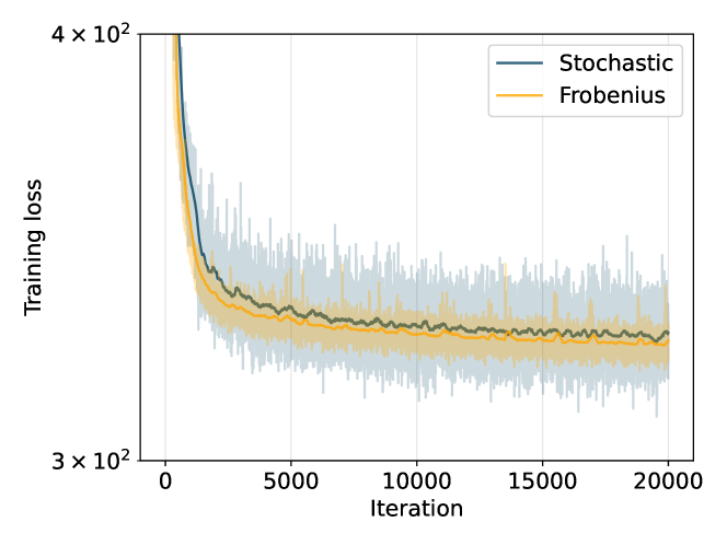
(a) Training loss

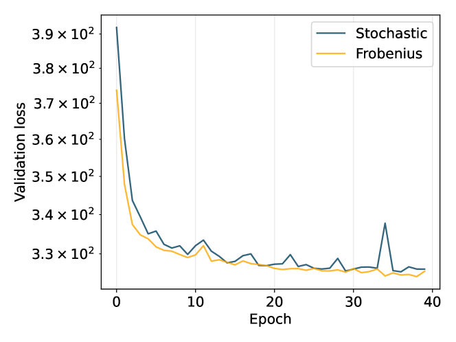
(b) Validation loss

Figure 6: Comparison of the training and validation loss for the Forbenius norm minimization and the stochastic approximation of the loss proposed by us. Here, we only compare the loss functions based on iteration count, not the actual time required to run the model training.

C.3 Scaling

Here, we are showing how our method scales in terms of computation time with respect to both the problem size. We compare the scaling of NeuralIF with the incomplete Cholesky method in Figure 7 using the PDE dataset as it contains a natural variety of differently sized problems. In the plot, we compare the number of non-zero matrix elements – which strongly correlates with the size of the matrix – with the time that is required to compute the preconditioner (P-time) (Figure 7(a)) as well as the time required to run the conjugate gradient method (Figure 7(b)) using both the smaller problem instances from the training process and the larger ones used for testing purposes.

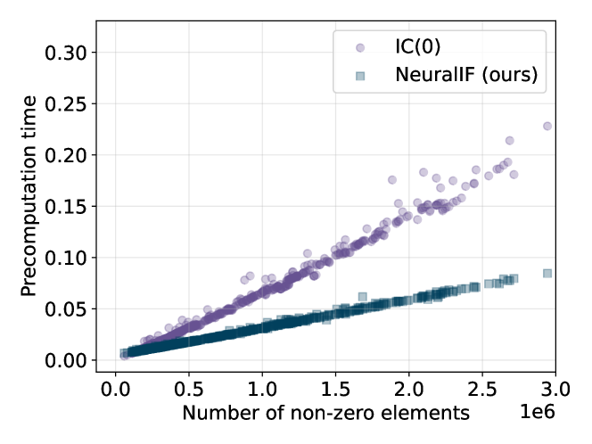
(a) Pre-computation time

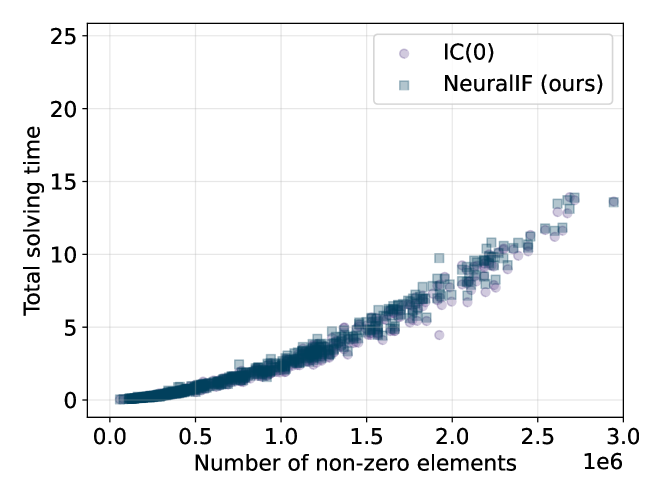
(b) Solving time

Figure 7: Comparison of the time required to compute the preconditioner (a) and solve the problem instance (b) with respect to the problem size – measured by the number of non-zero elements in the matrix ${\bm{A}}$ – for the incomplete Cholesky and our neural incomplete factorization (NeuralIF) method using 600 problem instances from the generated Poisson PDE problems. The generated outputs have by construction the same number of non-zero elements.

We can see that for small problem instances, the two methods lead to nearly the same time overhead required to compute the preconditioner. However, for larger problem instances with more than $1\thinspace 000\thinspace 000$ elements, our NeuralIF preconditioner clearly outperforms the incomplete Cholesky method in the time it is required to compute the preconditioner. Further, our method scales better when considering large problem instances. One possible explanation for this is that the overhead of our method is dominating the reported precomputation time for the small instances since the implementation of the GNN-based method is not optimized. For larger problems, this overhead becomes less relevant. However, larger problem instances are more interesting since the amortization of small instances is more difficult to start with. Further, our method leads to significantly less variance in the precomputation time. Further, we can see that for problems with large size, the precomputation time of the incomplete Cholesky method can vary a lot. In comparison, the neural network-based preconditioner is able to output the preconditioning matrix nearly in constant time for a given problem size. This is valuable since it allows a predictable cost to utilize our preconditioner when applying it to new problems.

For the time required to solve the problem – ignoring the previously spent time to compute the preconditioner – using the conjugate gradient method, we can see that both CG and NeuralIF perform very similar. The results, which are shown in Figure 7(b), show that the learned preconditioner clearly generalizes to the significantly larger problem instances and continues to produce well-performing preconditioners in terms of reduction in iterations and solving time of the CG algorithm.

Thus, in summary, we can see that the data-driven method is easier to compute and scales better for large problems while maintaining the performance of the incomplete Cholesky method in terms of the required solving time for the preconditioned problem.

C.4 PCG convergence

Synthetic problem  Here, additional results for the synthetic dataset are shown. Notably, Figure 8 shows the convergence of the different (preconditioned) CG runs on a single problem instance from the synthetic dataset where both the residual – which is also used as a stopping criterion – and the usually unavailable distance between the true solution and the iterate are shown. Further, for each problem the $\kappa({\bm{A}})$ worse case bound is displayed.

The distribution of the eigenvalues of the linear equation system – shown in Figure 3 in the main paper for this problem instance – directly influence the convergence behavior of the method. However, as it is commonly observed in the CG method, the $\kappa({\bm{A}})$-bound only describes the convergence behavior locally and overall, the algorithm converges significantly faster than the worst-case bound (Carson et al., 2023). We can, however, observe that the better conditioning still improves the convergence significantly and the obtained speedup is proportional to the speedup obtained in the worse-case bound making the condition number – at least for the problem instances considered in this dataset – a good measure for the performance of the conjugate gradient method. Further, we can see that our learned NeuralIF preconditioner is especially effective in the beginning of the CG algorithm and is able to outperform IC(0) for the first 100 iterations.

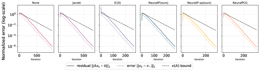
Figure 8: Convergence of the different preconditioned linear systems on a synthetic problem instance.

References

- Ackmann et al. (2021) Ackmann, J., Düben, P., Palmer, T., and Smolarkiewicz, P. Machine-Learned Preconditioners for Linear Solvers in Geophysical Fluid Flows. In EGU General Assembly Conference Abstracts, EGU General Assembly Conference Abstracts, pp. EGU21–5507, April 2021.
- Amos (2023) Amos, B. Tutorial on amortized optimization. Foundations and Trends in Machine Learning, 16(5):592–732, 2023. ISSN 1935-8237.
- Azulay & Treister (2022) Azulay, Y. and Treister, E. Multigrid-augmented deep learning preconditioners for the helmholtz equation. SIAM Journal on Scientific Computing, (0):S127–S151, 2022.
- Banert et al. (2021) Banert, S., Rudzusika, J., Öktem, O., and Adler, J. Accelerated forward-backward optimization using deep learning. arXiv preprint arXiv:2105.05210, 2021.
- Bansal et al. (2023) Bansal, D., Chen, R. T., Mukadam, M., and Amos, B. Taskmet: Task-driven metric learning for model learning. Advances in Neural Information Processing Systems, 2023.
- Battaglia et al. (2018) Battaglia, P. W., Hamrick, J. B., Bapst, V., Sanchez-Gonzalez, A., Zambaldi, V., Malinowski, M., Tacchetti, A., Raposo, D., Santoro, A., Faulkner, R., et al. Relational inductive biases, deep learning, and graph networks. arXiv preprint arXiv:1806.01261, 2018.
- Bengio et al. (2021) Bengio, Y., Lodi, A., and Prouvost, A. Machine learning for combinatorial optimization: a methodological tour d’horizon. European Journal of Operational Research, 290(2):405–421, 2021.
- Benzi (2002) Benzi, M. Preconditioning techniques for large linear systems: a survey. Journal of computational Physics, 182(2):418–477, 2002.
- Bronstein et al. (2021) Bronstein, M. M., Bruna, J., Cohen, T., and Veličković, P. Geometric deep learning: Grids, groups, graphs, geodesics, and gauges. arXiv preprint arXiv:2104.13478, 2021.
- Brualdi & Cvetkovic (2008) Brualdi, R. A. and Cvetkovic, D. A combinatorial approach to matrix theory and its applications. CRC press, 2008.
- Cai & Wang (2019) Cai, C. and Wang, Y. A simple yet effective baseline for non-attributed graph classification. ICLR Workshop: Representation Learning on Graphs and Manifolds, 2019.
- Cai et al. (2021) Cai, T., Luo, S., Xu, K., He, D., yan Liu, T., and Wang, L. Graphnorm: A principled approach to accelerating graph neural network training. International Conference on Machine Learning, 2021.
- Carson et al. (2023) Carson, E., Liesen, J., and Strakoš, Z. Solving linear algebraic equations with Krylov subspace methods is still interesting! arXiv preprint arXiv:2211.00953, 2023.
- Chen et al. (2022) Chen, T., Chen, X., Chen, W., Wang, Z., Heaton, H., Liu, J., and Yin, W. Learning to optimize: A primer and a benchmark. Journal of Machine Learning Research, 23(1), 2022.
- Chen et al. (2023) Chen, Z., Liu, J., Wang, X., and Yin, W. On representing linear programs by graph neural networks. In The Eleventh International Conference on Learning Representations, 2023.
- Chow & Patel (2015) Chow, E. and Patel, A. Fine-grained parallel incomplete lu factorization. SIAM journal on Scientific Computing, 37(2):C169–C193, 2015.
- Coates (1959) Coates, C. Flow-graph solutions of linear algebraic equations. IRE Transactions on Circuit Theory, 6(2):170–187, 1959.
- Davis et al. (2016) Davis, T. A., Rajamanickam, S., and Sid-Lakhdar, W. M. A survey of direct methods for sparse linear systems. Acta Numerica, 25:383–566, 2016.
- Doob (1984) Doob, M. Applications of graph theory in linear algebra. Mathematics Magazine, 57(2):67–76, 1984.
- Dudzik & Veličković (2022) Dudzik, A. J. and Veličković, P. Graph neural networks are dynamic programmers. Advances in Neural Information Processing Systems, 35:20635–20647, 2022.
- Fey & Lenssen (2019) Fey, M. and Lenssen, J. E. Fast graph representation learning with PyTorch Geometric. In ICLR Workshop on Representation Learning on Graphs and Manifolds, 2019.
- Golub & Van Loan (2013) Golub, G. H. and Van Loan, C. F. Matrix computations. JHU press, 2013.
- Gonzaga de Oliveira et al. (2018) Gonzaga de Oliveira, S. L., Bernardes, J., and Chagas, G. An evaluation of reordering algorithms to reduce the computational cost of the incomplete Cholesky-conjugate gradient method. Computational and Applied Mathematics, 37:2965–3004, 2018.
- Grementieri & Galeone (2022) Grementieri, L. and Galeone, P. Towards Neural Sparse Linear Solvers. arXiv preprint arXiv:2203.06944, 2022.
- Gustafsson & McBain (2020) Gustafsson, T. and McBain, G. D. scikit-fem: A Python package for finite element assembly. Journal of Open Source Software, 5(52):2369, 2020.
- Götz & Anzt (2018) Götz, M. and Anzt, H. Machine learning-aided numerical linear algebra: Convolutional neural networks for the efficient preconditioner generation. In 2018 IEEE/ACM 9th Workshop on Latest Advances in Scalable Algorithms for Large-Scale Systems (scalA), pp. 49–56, 2018.
- Hofreither (2020) Hofreither, C. ilupp – ilu algorithms for c++ and python, 2020. URL https://github.com/c-f-h/ilupp.
- Hutchinson (1989) Hutchinson, M. F. A stochastic estimator of the trace of the influence matrix for laplacian smoothing splines. Communications in Statistics-Simulation and Computation, 18(3):1059–1076, 1989.
- Jenatton et al. (2011) Jenatton, R., Audibert, J.-Y., and Bach, F. Structured variable selection with sparsity-inducing norms. The Journal of Machine Learning Research, 12:2777–2824, 2011.
- Kaneda et al. (2023) Kaneda, A., Akar, O., Chen, J., Kala, V., Hyde, D., and Teran, J. A deep gradient correction method for iteratively solving linear systems. International Conference in Machine Learning, 2023.
- Langtangen & Logg (2016) Langtangen, H. P. and Logg, A. Solving PDEs in minutes-the FEniCS tutorial I, volume 3 of Simula SpringerBriefs on Computing. Springer, 2016.
- Li et al. (2023) Li, Y., Chen, P. Y., Matusik, W., et al. Learning preconditioner for conjugate gradient pde solvers. International Conference in Machine Learning, 2023.
- Lin & Moré (1999) Lin, C.-J. and Moré, J. J. Incomplete Cholesky factorizations with limited memory. SIAM Journal on Scientific Computing, 21(1):24–45, 1999.
- Martinsson & Tropp (2020) Martinsson, P.-G. and Tropp, J. A. Randomized numerical linear algebra: Foundations and algorithms. Acta Numerica, 29:403–572, 2020.
- Mayer (2007) Mayer, J. Ilu++: A new software package for solving sparse linear systems with iterative methods. In PAMM: Proceedings in Applied Mathematics and Mechanics, volume 7, pp. 2020123–2020124. Wiley Online Library, 2007.
- Moore et al. (2023) Moore, N. S., Cyr, E. C., Ohm, P., Siefert, C. M., and Tuminaro, R. S. Graph neural networks and applied linear algebra. arXiv preprint arXiv:2310.14084, 2023.
- Nocedal & Wright (1999) Nocedal, J. and Wright, S. J. Numerical optimization. Springer, 1999.
- Nytko et al. (2022) Nytko, N., Taghibakhshi, A., Zaman, T. U., MacLachlan, S., Olson, L. N., and West, M. Optimized sparse matrix operations for reverse mode automatic differentiation. arXiv preprint arXiv:2212.05159, 2022.
- Paszke et al. (2019) Paszke, A., Gross, S., Massa, F., Lerer, A., Bradbury, J., Chanan, G., Killeen, T., Lin, Z., Gimelshein, N., Antiga, L., et al. Pytorch: An imperative style, high-performance deep learning library. Advances in neural information processing systems, 32, 2019.
- Pearson & Pestana (2020) Pearson, J. W. and Pestana, J. Preconditioners for Krylov subspace methods: An overview. GAMM-Mitteilungen, 43(4), November 2020. ISSN 0936-7195, 1522-2608.
- Potra & Wright (2000) Potra, F. A. and Wright, S. J. Interior-point methods. Journal of Computational and Applied Mathematics, 124(1):281–302, 2000. ISSN 0377-0427. Numerical Analysis 2000. Vol. IV: Optimization and Nonlinear Equations.
- Saad (1994) Saad, Y. Ilut: A dual threshold incomplete lu factorization. Numerical linear algebra with applications, 1(4):387–402, 1994.
- Saad (2003) Saad, Y. Iterative Methods for Sparse Linear Systems. SIAM, Philadelphia, 2nd edition, 2003. ISBN 978-0-89871-534-7.
- Sappl et al. (2019) Sappl, J., Seiler, L., Harders, M., and Rauch, W. Deep learning of preconditioners for conjugate gradient solvers in urban water related problems. arXiv preprint arXiv:1906.06925, 2019.
- Scott & Tůma (2023) Scott, J. and Tůma, M. Algorithms for Sparse Linear Systems. Springer International Publishing, Cham, 2023.
- Shewchuk (1994) Shewchuk, J. R. An introduction to the conjugate gradient method without the agonizing pain. Carnegie-Mellon University. Department of Computer Science Pittsburgh, 1994.
- Sjölund & Bånkestad (2022) Sjölund, J. and Bånkestad, M. Graph-based neural acceleration for nonnegative matrix factorization. arXiv preprint arXiv:2202.00264, 2022.
- Stanaityte (2020) Stanaityte, R. ILU and Machine Learning Based Preconditioning For The Discretized Incompressible Navier-Stokes Equations. PhD thesis, University of Houston, 2020.
- Stellato et al. (2020) Stellato, B., Banjac, G., Goulart, P., Bemporad, A., and Boyd, S. OSQP: An operator splitting solver for quadratic programs. Mathematical Programming Computation, 12(4):637–672, 2020.
- Tang et al. (2022) Tang, Z., Zhang, H., and Chen, J. Graph Neural Networks for Selection of Preconditioners and Krylov Solvers. NeurIPS 2022 New Frontiers in Graph Learning Workshop, 2022.
- Veličković (2023) Veličković, P. Everything is connected: Graph neural networks. Current Opinion in Structural Biology, 79:102538, 2023.
- Vemulapalli & Jacobs (2015) Vemulapalli, R. and Jacobs, D. W. Riemannian metric learning for symmetric positive definite matrices. arXiv preprint arXiv:1501.02393, 2015.