Model-independent reconstruction of the Interacting Dark Energy Kernel:
Binned and Gaussian process

Abstract

The cosmological dark sector remains an enigma, offering numerous possibilities for exploration. One particularly intriguing option is the (non-minimal) interaction scenario between dark matter and dark energy. In this paper, to investigate this scenario, we have implemented Binned and Gaussian model-independent reconstructions for the interaction kernel alongside the equation of state; while using data from BAOs, Pantheon+ and Cosmic Chronometers. In addition to the reconstruction process, we conducted a model selection to analyze how our methodology performed against the standard $\Lambda$CDM model. The results revealed a slight indication, of at least 1$\sigma$ confidence level, for some oscillatory dynamics in the interaction kernel and, as a by-product, also in the DE and DM. A consequence of this outcome is the possibility of a sign change in the direction of the energy transfer between DE and DM and a possible transition from a negative DE energy density in early-times to a positive one at late-times. While our reconstructions provided a better fit to the data compared to the standard model, the Bayesian Evidence showed an intrinsic penalization due to the extra degrees of freedom. Nevertheless these reconstructions could be used as a basis for other physical models with lower complexity but similar behavior.

I INTRODUCTION

Over the course of more than two decades there has been an avalanche of theoretical studies and data analysis to understand the fundamental nature of the dark energy (DE), nevertheless so far it still remains as an open question. This mysterious component of the universe was initially introduced as a possibility to explain the current accelerated expansion of the Universe, discovered through the Type Ia Supernovae (SN) observations [1, 2, 3, 4], and then confirmed by different measurements, like the Cosmic Microwave Background (CMB) anisotropies [5, 6, 7, 8] or the Baryon Acoustic Oscillations (BAO) [9, 10, 11, 12, 13]. In its simplest form, the DE is assumed to be a cosmological constant ($\Lambda$) incorporated into the Einstein field equations (EFEs). It is equivalent to the usual vacuum energy density of the quantum field theory, described as a perfect fluid with a barotropic equation of state parameter (EoS) $w_{\mathrm{DE}}=p/\rho$, with $w_{\Lambda}=-1$. The cosmological constant, along with the cold dark matter (CDM), a key component for structure formation in the Universe, plays a crucial role in setting up the standard cosmological model, best known as Lambda Cold Dark Matter ($\Lambda$CDM) model. Even though this model is able to explain, with great accuracy, most of the contemporary observations, it exhibits some issues on theoretical grounds, like the Cosmological Constant problem [14, 15, 16, 15] and the Coincidence problem [17, 18, 19]; and also faces some difficulties on the observational side, viz., the $H_{0}$ tension [20, 21, 22, 23, 24, 25, 26], and the $\sigma_{8}-S_{8}$ tension [27, 28] (see also [29] for a review of the current tensions and anomalies in cosmology). In order to explain the small scale structure formation, or at least to ameliorate the problems associated with the CDM model, several alternatives have been introduced. One viable option is to replace the standard CDM with Scalar Field dark matter components [30, 31, 32, 33, 34, 35] or by introducing the Self Interacting dark matter [36, 37, 38], or to support the warm dark matter scenario [39, 40]. Regarding the current accelerated expansion of the Universe, a natural extension to the constant EoS is introducing phenomenological dynamics to model the general behavior of the DE, whose main methodology relies on giving a functional form with a dependence on redshift/scale factor, i.e., $w_{\mathrm{DE}}=w(z)$, see, e.g., [41, 42, 43, 44, 45]. For instance, parametric forms of the EoS parameter $w_{\mathrm{DE}}$ have been studied extensively throughout several papers, as they served as guidelines to uncover some underlying issues from the theory, and are commonly referred to as Dynamical Dark Energy (DDE) parameterizations. One of the simplest descriptions of $w_{\mathrm{DE}}$ is given by a Taylor series in terms of the scale factor $a$, and a set of free parameters, i.e., $w_{0}$ and $w_{a}$, whose particular cases are the $w$CDM model, $w_{\mathrm{DE}}=w_{0}$, and the Chevallier-Polarski-Linder (CPL) parametrization, $w_{\mathrm{DE}}=w_{0}+w_{a}\left(1-a\right)$ [46, 47, 48, 49, 50], or it could be carried out in terms of redshift $z$ [51], or cosmic time $w_{\mathrm{DE}}=w_{0}+w_{a}(1-t)$ [52], or in general by using another basis of series expansion, e.g., a Fourier-base [53]. There are also more complex parameterizations that may include combinations of power laws, exponentials, logarithms and trigonometrics components [54, 55, 56, 57, 58, 59]. Studies of the equation of state have been very useful to describe the DE features, nevertheless, several works have extended the search by looking for deviations from the constant energy density $\rho_{\mathrm{DE}}$. Examples of these investigations include the Graduated dark energy (gDE) [60, 61, 62, 63, 64], the Phantom crossing [65], Omnipotent dark energy [66] or the Early dark energy [67], just to mention a few. Also, some of the possibilities that replace the cosmological constant include canonical scalar fields like quintessence, phantom or a combination of multi-fields named quintom models [68, 69, 70, 71, 72, 73, 74, 75]; or it could even be modifications that go beyond the General Relativity such as $f(R)$ theories [76, 77] or braneworld models [78, 79, 80, 81].

On the other hand, there exists a particular type of models where the non-minimal interaction (hereinafter we use the word interaction to mean non-minimal interaction) between DM and DE may be able to solve or at least alleviate these issues with relative ease [82, 83, 84, 85, 86, 87, 88, 89, 90, 91, 92, 93, 94, 95, 96, 97, 98]. Recent analyses have focused on the resemblance between DM-DE interacting models with modified gravity theories [99, 100, 101, 102]. Also, a viable alternative is to assume a interaction between these two components [103, 104].

Even though the interacting models have been extensively analyzed, their interaction kernel still remains a mystery. This is why a significant amount of research works has been dedicated to introducing new models in a phenomenological way, such as the parameterizations. Models with interacting dark sectors, also named Interacting Dark Energy (IDE), are no strangers to parameterizations, since the interplay is generally proposed in a particular demeanor motivated by certain characteristics. For example, a popular assumption, inspired by several behaviors in particle physics [105], is to express the interaction kernel, $Q$, in terms of the energy densities ($\rho_{\rm DM}$ and/or $\rho_{\rm DE}$) and time (through the Hubble parameter $H^{-1}(z)$). Nevertheless, these are only few assumptions and, since the nature of the interaction is still obscure, they can come up in several different functional forms and combinations, see for example [83, 84, 99, 89, 91, 106]. Generally, for these type of models, it is found that the structure formation remains unaltered and late-time acceleration is also in accordance with the standard model (see [99, 104] for a comprehensive review of interacting models and their behavior).

However, as useful as parameterizations may be (not only for DDE or IDE but in general) they posses certain limitations. One of this is that a functional form is assumed a priori which could bias the results. For example selecting a phantom or quintessence like component remarks a clear difference in the DE behavior when choosing a particular parameterization. Another limitation was demonstrated in [107]; expansions in small parameters are more influenced by higher redshift data, whereas data from lower redshifts carry less weight in the analysis. A possible way to avoid these issues it to perform reconstructions by extracting information directly from the data, using model-independent techniques or non-parametric ones, such as Artificial Neural Networks [108, 109, 110], Gaussian Process [111, 112, 113, 114, 115, 116, 110, 117, 118] or, recently, we can see applications of binning, linear interpolations and the incorporation of a correlation function in [119]. The Gaussian process (GP), specifically for the IDE models, has become a regular choice for a non-parametric approach [120, 121, 122, 123, 124, 125]. This methodology has found a possibility of an interaction and given some insights into possible preferred behaviors and characteristics, such as a crossing of the non-interacting line. In spite of this, the GP approach cannot be used for model comparison in concordance with the $\Lambda$CDM model given its non-parametric nature.

Despite the extensive study of both the interaction models and the model-independent approaches in cosmology, they have been rarely used in tandem, at least to our knowledge; for example Cai et. al. [126] and Salvatelli et. al. [127] used redshift bins, and for Solano et. al. [128] the main focus are the Chebyshev polynomials. They found a possible crossing in the non interaction line, and in [126] obtained an oscillatory behavior through the interaction, although the data in this work was limited to cover a narrow range of redshift (around $z<1.8$). This finding inspired the study of possible sign-switching interactions, instead of the classical monotonically decreasing or increasing parameterizations. We have for example: in [129] the parameterization $Q(a)=3b(a)H_{0}\rho_{0}$ was first proposed, with $b(a)=b_{0}a+b_{e}(1-a)$ being the sign-switching part; in [130] the model $Q=3H\sigma(\rho_{\rm DE}-\alpha\rho_{\rm DM})$ ($\alpha$ being a positive constant of order unity) also presents a switching interaction; in [131] the named Ghost dark energy is used in tandem with an interaction kernel $Q=3\beta Hq(\rho_{\rm DE}+\rho_{\rm DM})$ where its sign is able to change since it is a function of the deceleration parameter $q$; and in [132] a bunch of variations of $Q(a)=3b(a)H(a)\rho_{i}$ are studied. The general consensus reached by the majority of these models is that, if a transition were to happen, it should be around the time when the accelerated expansion of the Universe began ($z\sim 0.5$). Therefore, in this work we will use some model-independent approaches to reconstruct the interaction kernel between DE and DM directly from the data. The methods used (as will be explained in the next sections) are the binning scheme along with the Gaussian Process as an interpolation approach. Moreover, as additional cases, together with the DM-DE interaction, we will replace the cosmological constant with a constant EoS free to vary.

The paper is organized as follows: in Section II we provide a brief review of the underlying theoretical reason that led us to consider the possibility of non-minimal interaction within the dark sector, followed by Section III where we describe the reconstruction methodologies. In Section IV the datasets and some specifications about the parameter estimation and model selection are made clear. In Section V we present the main results, and finally in Section VI we give our conclusions.

II INTERACTING DM-DE MODEL

In the general theory of relativity (GR), the Einstein field equations can be written as $G_{\mu\nu}=\kappa T_{\mu\nu}^{\rm tot}$, where $\kappa=8\pi G$ ($G$ is Newton’s constant), $G_{\mu\nu}$ is the Einstein tensor, and $T_{\mu\nu}^{\rm tot}$ is the total energy-momentum tensor (EMT), viz., the sum of the EMTs of sources such as radiation (photons and neutrinos), baryons, CDM/DM, and DE, which constitute the physical content of the universe. It is an important feature of the EFEs that the twice contracted Bianchi identity, $\nabla^{\mu}G_{\mu\nu}=0$, implies the conservation of the total EMT, i.e., $\nabla^{\mu}T_{\mu\nu}^{\rm tot}=0$. Accordingly, in a relativistic cosmological model assuming the spatially flat Robertson-Walker spacetime, in the presence of sources in the standard model of particle physics—i.e., baryons ($w_{\rm b}=0$), radiation (photons and neutrinos) ($w_{\rm r}=\frac{1}{3}$)—and sources of unknown nature—CDM ($w_{\rm CDM}=w_{\rm DM}=0$) and DE ($w_{\rm DE}$ is left unspecified)—the EFEs lead to the following Friedmann and continuity equations, respectively:

$$3H^{2}=\kappa(\rho_{\rm r}+\rho_{\rm b}+\rho_{\rm DM}+\rho_{\rm DE}),$$ (1)

$$\begin{aligned} \dot{\rho}_{\rm r}+4H\rho_{\rm r}+\dot{\rho}_{\rm b}&+3H\rho_{\rm b}+\dot{\rho}_{\rm DM}+3H\rho_{\rm DM}\\ &+\dot{\rho}_{\rm DE}+3H\rho_{\rm DE}(1+w_{\rm DE})=0,\end{aligned}$$ (2)

where $H$ is the Hubble parameter, and a dot denotes derivative with respect to cosmic time. It is reasonable to assume that the sources such as baryons and radiation, whose physics are well known within the standard model of particle physics, are individually conserved, i.e., $\nabla^{\mu}T_{\mu\nu}^{\rm r}=0$ and $\nabla^{\mu}T_{\mu\nu}^{\rm b}=0$ (viz., $\dot{\rho}_{\rm r}+4H\rho_{\rm r}=0$ and $\dot{\rho}_{\rm b}+3H\rho_{\rm b}=0$). This in turn implies, via continuity equation Eq. 2, conservation within the dark sector (DM+DE) itself:

$$\dot{\rho}_{\rm DM}+3H\rho_{\rm DM}+\dot{\rho}_{\rm DE}+3H\rho_{\rm DE}(1+w_{\rm DE})=0.$$ (3)

At this stage, in the cosmology literature so far, the very strong assumption that DM and DE are conserved separately—i.e., $\dot{\rho}_{\rm DM}+3H\rho_{\rm DCM}=0$ and $\dot{\rho}_{\rm DE}+3H\rho_{\rm DE}(1+w_{\rm DE})=0$—is often made with almost no basis of this assumption. Then, taking advantage of the only remained freedom, viz., $w_{\rm DE}$, due to the unknown nature of DE, different models of DE have been put forward to extend the standard cosmological model since the discovery of the late time acceleration of the Universe. Thus, if we do not follow this two-step path to build a cosmological model, the fact that the nature of both DM and DE are still unknown and GR itself does not impose them to be conserved separately, we have, from Eq. 3, $\nabla^{\mu}T_{\mu\nu}^{\rm DM}=-Q$ and $\nabla^{\mu}T_{\mu\nu}^{\rm DE}=-Q$, namely,

$$\dot{\rho}_{\rm DM}+3H\rho_{\rm DM} =Q,$$ (4)

$$\dot{\rho}_{\rm DE}+3H\rho_{\rm DE}(1+w_{\rm DE}) =-Q,$$ (5)

where we have two undetermined functions; the DE EoS parameter $w_{\rm DE}$ and the interaction kernel $Q$, which determines the rate and direction of the possible energy transfer between DE and DM; namely, $Q=0$ implies minimal interaction (gravitational interaction only) between DM and DE, $Q>0$ implies energy transfer from DE to DM, and $Q<0$ implies energy transfer from DM to DE. In particular, in the case $Q=0$ (minimal interaction) and $w_{\rm DE}=-1$ we have the standard $\Lambda$CDM model. In this work, we will not impose any phenomenological or theoretical models for the nature of interaction between DM and DE [viz., $Q(z)$] and the dynamics of the DE [viz., $w_{\rm DE}$, or a corresponding $\rho_{\rm DE}(z)$], instead we will reconstruct these parameters, as well as some important kinematic parameters [viz., the Hubble parameter $H(z)$ and deceleration parameter $q(z)\equiv-1+{\rm d}H(z)^{-1}/{\rm d}t$], from observational data in a model-independent manner. The effects of a possible non-minimal interaction between DM and DE will be reflected on altered kinematics of the universe. This can be observed via the Friedmann equation (2), due to the deviations in the evolution of the energy densities of the DM and DE from what they would have in the absence of a non-minimal interaction. It is in general very useful to have an idea on what corresponding minimally interacting (no energy exchange) DE and DM would lead to the same altered kinematics of the universe. To do so, we will define effective EoS parameters for the DM and DE; $w_{\rm eff,\rm DM}$ and $w_{\rm eff,\rm DE}$, respectively. These effective parameters are defined such that, in the absence of non-minimal interaction, they would lead to the same functional forms $\rho_{\rm eff,\rm DE}$ and $\rho_{\rm eff,\rm DE}$ as obtained through the model-independent reconstruction processes by allowing a possible non-minimal interaction. Accordingly, we write the following separate continuity equations for the DM and DE in terms of $w_{\rm eff,\rm DE}$ and $w_{\rm eff,\rm DM}$

$$\dot{\rho}_{\rm DM}+3H(1+w_{\rm eff,DM})\rho_{\rm DM}=0,$$ (6)

$$\dot{\rho}_{\rm DE}+3H(1+w_{\rm eff,DE})\rho_{\rm DE}=0,$$ (7)

and then, comparing these with the continuity equations that involve the interaction kernel, i.e., Eqs. 4 and 5, we reach the following relation between the effective EoS parameters of the DM and DE and the interaction kernel:

$$w_{\rm eff,\rm DM}=\frac{-Q}{3H\rho_{\rm DM}},\quad w_{\rm eff,\rm DE}=w_{\rm DE}+\frac{Q}{3H\rho_{\rm DE}}.$$ (8)

It is also convenient to define a dimensionless interaction kernel parameter as follows;

$$\Pi_{\rm DM}=\frac{-Q}{3H\rho_{\rm c,0}}=-\Pi_{\rm DE},$$ (9)

where $\rho_{\rm c,0}=3H_{0}^{2}/8\pi G$ is the critical energy density of the present-day universe. Now, let’s see how $Q=Q(z)$ should behave so that we can choose appropriate priors for the reconstruction. It is widely accepted that, despite its problems, $\Lambda$CDM is very good at explaining most observations, so our efforts should not differ significantly from it, despite the model-independent nature of the reconstructions used. For a comprehensive understanding of the impact of this interaction, perturbation analysis should also be included in our analysis. However, our focus in this study, as a proof of the concept, is on the background data and therefore we leave the full analysis including perturbations for future research. On the other hand, this does not mean that perturbations have been completely ignored here, as their effects are already reflected when choosing the prior ranges for $\Pi_{\rm DE}$. In order to preserve the dust-like behavior of the DM and avoid significantly altering the perturbations, thus not spoiling the structure formation, one may demand that $w_{\rm eff,DM}\sim 0$ [133, 104, 99], which implies $|\frac{Q}{3H\rho_{\rm DM}}|\sim 0$, then $|\frac{Q}{3H}|\ll\rho_{\rm DM}$. Namely, we cannot have $\frac{Q}{3H}\sim\rho_{\rm DM}>0$ otherwise the Universe would always remain in the matter dominated era (viz., in the Einstein-de Sitter universe phase). Also, it is preferable to prevent $\frac{Q}{3H}<0$ and $|\frac{Q}{3H}|\sim\rho_{\rm DM}$ otherwise the Universe would have never entered the matter dominated era and the successful explanation of galaxy and large-scale structure formation would be spoiled. With some algebra and using our definitions we arrive at $|\Pi_{\rm DE}|\ll\Omega_{\rm m}\frac{H^{2}}{H_{0}^{2}}$. Recent studies [96, 134] found that when using current cosmological data, the interaction could be so intense as to imply $w_{\rm eff,DM}\sim 1/3$. We will make use of these results as a motivation to relax the constrain on $\Pi_{\rm DE}$, so we will allow $|\Pi_{\rm DE}|\sim\Omega_{\rm m}\frac{H^{2}}{H_{0}^{2}}$. These restrictions will be used as a guide when proposing the priors for the reconstruction of $\Pi_{\rm DE}(z)$ in Section III and, when displaying the reconstructed $\Pi_{\rm DE}$, we will plot the curve $\Omega_{\rm m}H^{2}/H_{0}^{2}$ as a reference.

By using the dimensionless interaction kernel together with the chain rule and $\rho_{\rm c,0}$, we can express Eqs. 4 and 5 as

$$\frac{{\rm d}(\rho_{\rm DM}/\rho_{\rm c,0})}{{\rm d}z} =\frac{3}{1+z}\bigg{(}\frac{\rho_{\rm DM}}{\rho_{\rm c,0}}+\Pi_{\rm DM}\bigg{)},$$ (10a)

$$\frac{{\rm d}(\rho_{\rm DE}/\rho_{\rm c,0})}{{\rm d}z} =\frac{3}{1+z}\bigg{[}(1+w_{\rm DE})\frac{\rho_{\rm DE}}{\rho_{\rm c,0}}+\Pi_{\rm DE}\bigg{]},$$ (10b)

respectively. These continuity equations are then solved numerically and used to express our Friedmann equation, i.e., $H(z)$. The continuity equations for radiation and baryonic matter do not change, so we have, assuming a spatially flat universe:

$$\frac{H^{2}(z)}{H_{0}^{2}}=\Omega_{b,0}(1+z)^{3}+\frac{\rho_{\rm DM}(z)}{\rho_{\rm c,0}}+\frac{\rho_{\rm DE}(z)}{\rho_{\rm c,0}},$$ (11)

where we have neglected radiation, as it is well negligible in the post-recombination universe.

In [135] it was demonstrated that an equivalence between dynamical DE (through a dynamical EoS parameter) and an interacting DE-DM model (with a constant EoS parameter) exists at the background level. To avoid this and to maintain as little bias as possible regarding the underlying possible functional form of the dimensionless interaction kernel parameter $\Pi_{\rm DE}(z)$, our reconstruction efforts will be aimed mainly towards the interaction kernel but letting the EoS parameter to be a variable single bin $w_{0}$. Reconstructing both functions with model independent approaches, with a large number of extra parameters at the same time, could lead to a lot of degeneracies with Eq. 8, but it may be worth to do it in future works.

Finally, for the sake of comparison we will also plot Solano’s dimensionless interaction function [128]:

$$I_{Q}(z)=\frac{Q(z)}{\rho_{\rm c,0}H(z)(1+z)^{3}},$$ (12)

which is proposed as a way to better visualize the interaction kernel and its defining characteristics.

III BINNED AND GAUSSIAN PROCESS INTERPOLATIONS

One of the reconstruction methods considered in this paper, to describe $f(z)$, consists in using a set of step functions connected via hyperbolic tangents to maintain smooth continuity. The function to reconstruct then takes the following form:

$$f(z)=f_{1}+\sum^{N-1}_{i=1}\frac{f_{i+1}-f_{i}}{2}\bigg{[}1+\tanh{\Big{(}\frac{z-z_{i}}{\xi}\Big{)}}\bigg{]},$$ (13)

where $N$ is the number of bins, $f_{i}$ the amplitude of the bin value, $z_{i}$ the position where the bin begins in the $z$ axis and $\xi$ the smoothness parameter, set to $\xi=0.15$ in this work.

The other approach is an interpolation by using a Gaussian Process (GP). A GP is the generalization of a Gaussian distribution, that is, in every position $x$, $f(x)$ is a random variable. It is characterized by a mean function $\mu(x)$ and a covariance $\sigma^{2}K(x,x^{\prime})$, where $\sigma^{2}$ is the variance and $K(x,x^{\prime})$ the kernel representing the correlation of $f$ between two different positions $f(x)$ and $f(x^{\prime})$. For an arbitrary amount of positions $x_{1},..,x_{n}$ then we have a multivariate Gaussian distribution

$$\bar{f}=[f(x_{1}),..,f(x_{n})]\leavevmode\nobreak\ \bar{N}(\bar{\mu},\sigma^{2}K(\bar{x},\bar{x^{\prime}})),$$ (14)

where $\bar{\mu}=[\mu(x_{1}),...,\mu(x_{n})]$, and

$$K(\bar{x},\bar{x}^{\prime})=\begin{pmatrix}K(x_{1},x_{1})&K(x_{1},x_{2})&\cdots&K(x_{1},x_{n})\\ K(x_{2},x_{1})&K(x_{2},x_{2})&\cdots&K(x_{2},x_{n})\\ \vdots&\vdots&\ddots&\vdots\\ K(x_{n},x_{1})&K(x_{n},x_{2})&\cdots&K(x_{n},x_{n})\end{pmatrix}.$$ (15)

The Kernel we will use in this work is the Radial Basis Function (RBF)

$$K(x,x^{\prime})={\rm exp}\big{[}-\theta(x-x^{\prime})^{2}\big{]},$$ (16)

where the parameter $\theta$ tells us how strong is the correlation. This kernel has the advantage of minimizing the degeneracies created due to a high number of hyperparameters since it only has $\theta$, it is isotropic if we choose $x=z$ being $z$ the cosmological redshift, and it is also infinitely differentiable.

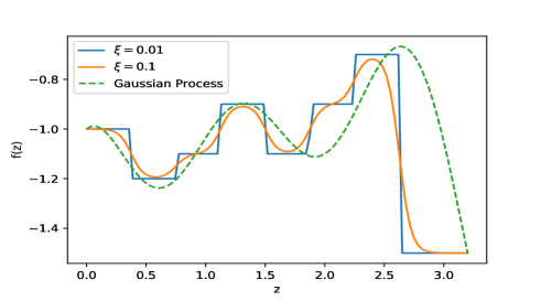
Figure 1: Comparison between a Gaussian Process for interpolation and a step function approach. The influence of the smoothness parameter $\xi$ in the Binning scheme is also shown.

Analogous to the binning approach, the GP will be used as an interpolation between nodes in order to have a model-independent reconstruction in a similar fashion as the reconstruction performed in [136]. This method yields to slightly different results as seen in Fig. 1. We will have node values located at $z_{i}$ to described $\Pi_{\rm DE}(z_{i})$. The $z_{i}$ values remained fixed, so the free parameters for our interaction kernel would be the amplitudes $\Pi_{\rm DE}(z_{i})=\Pi_{i}$.

In the present work, and without loss of generality, for the reconstruction of $\Pi_{\rm DE}$ we will utilize five amplitudes, evenly located across the interval of $0.0\leq z\leq 3.0$. This choice implies that each amplitude encompasses a redshift interval of 0.6 when using bins. Alternatively, when utilizing GP the positions of the amplitudes $\Pi_{i}$ are located in the following positions $[0.0,0.75,1.5,2.25,3.0]$.

IV DATASETS AND METHODOLOGY

In this work, we will use the collection of cosmic chronometers [137, 138, 139, 140, 141, 142, 143] (we will refer to this dataset as H), which can be found within the repository [144]. We also make use of the full catalogue of supernovae from the Pantheon+ SN Ia sample, covering a redshift range of $0<z\lesssim 2.26$ [145] (we will refer to this dataset as SN). The full covariance matrix associated is comprised of a statistical and a systematic part, and along with the data, they are provided in the repository [146]. Finally we also employ the BAO datasets, containing the SDSS Galaxy Consensus, quasars and Lyman-$\alpha$ forests [147]. The sound horizon is calibrated by using BBN [148]. For a more detailed description of the datasets refer to [119]. We will call this dataset BAO.

Table 1: Jeffreys’ scale for model selection with the logarithm of the Bayes’ factor. Using the convention from [149].

$\ln{B_{12}}$	Odds	Probability	Strength of evidence
$<$ 1.0	$<$3:1	$<$0.75	Inconclusive
1.0	$\sim$3:1	0.750	Weak evidence
2.5	$\sim$12:1	0.923	Moderate evidence
5.0	$\sim$150:1	0.993	Strong evidence

To find the best-fit values for the free parameters of our model, we use a modified version of the Bayesian inference code, called SimpleMC [150, 151], used for computing expansion rates and distances from the Friedmann equation. For a model $i$ we have computed its Bayesian evidence $E_{i}$, and to compare two different models (1 and 2) we make use of the Bayes’ factor $B_{1,2}=E_{1}/E_{2}$, specifically its natural logarithm. When used in tandem with the empirical Jeffreys’ scale, Table 1, we can have a better notion of the alternative models’ performance. To evaluate the fitness of our reconstructions (with respect to $\Lambda$CDM) we will make use of the $-2\ln\mathcal{L_{\rm max}}$ of each model, where $\mathcal{L_{\rm max}}$ is the maximum likelihood obtained (in the Bayesian sense). The SimpleMC code includes the dynesty library [153], a nested sampling algorithm used to compute the Bayesian evidence. The number of live-points were selected using the general rule $50\times ndim$ [154], where $ndim$ is the number of parameters to be sampled. The flat priors used for the base parameters are: $\Omega_{\rm m}=[0.1,0.5]$ for the matter density parameter, $\Omega_{\rm b}h^{2}=[0.02,0.025]$ for the physical baryon density, $h=[0.4,0.9]$ for the dimensionless Hubble constant $h=H_{0}/100\,{\rm km\,s}^{-1}{\rm Mpc}^{-1}$. For comparison we include the $w$CDM model $w_{\rm DE}(z)$$=w_{c}$, the Chevallier-Polarski-Linder (CPL) EoS parameter $w_{\rm DE}(z)$$=w_{0}+w_{a}\frac{z}{1+z}$ [46] and the sign-switch interaction kernel (SSIK) $Q=3\sigma H(\rho_{\rm DE}-\alpha\rho_{\rm DM})$ [130]. Their free parameters being $w_{c}$, $w_{0}$ and $w_{a}$ for $w$CDM and CPL; for SSIK $w_{0}=[-2.0,0.0]$, $\sigma=[0.0,1.0]$ and $\alpha=[0,4]$. The flat prior for $w_{c}$, and $w_{0}$, is the same $[-2.0,0.0]$ and the flat prior used for $w_{a}$ is $[-2.0,2.0]$. For the reconstruction of $\Pi_{\rm DE}(z)$ we recall that $|\Pi_{\rm DE}|\ll\Omega_{\rm m}(z)E^{2}(z)$, with $E(z)\equiv\frac{H(z)}{H_{0}}$, also that generally $\Omega_{\rm m}(0)\approx 0.3$, and as we move from late-times to early-times this value only grows. We will use $|\Pi_{\rm DE}|\sim\Omega_{\rm m}(z)E^{2}(z)$ as a loose guide as mentioned before to choose our priors, we have then $\Pi_{\rm DE,i}=[-2.0,2.0]$ when $z<1.0$ and $\Pi_{\rm DE,i}=[-15.0,15.0]$ when $z>1.0$ . Regarding the EoS parameter we either fix it to a cosmological constant $w_{0}=-1$ or let it vary as a free parameter $w_{0}=[-2.0,0.0]$.

V RESULTS

In this section we present the constraints, at 68% CL, for $h$ and $\Omega_{\rm m}$, along with a comparison of the best-fit of the model $-2\Delta\ln\mathcal{L_{\rm max}}$ and the Bayes Factor, with respect to $\Lambda$CDM, shown in Table 2 for all the scenarios. Moreover, we show the posterior probability density functions, at 68% and 95% CL, for some quantities of interest in the interacting scenarios in Figs. 2, 3, 4 and 5.

Beginning with the well known parameterizations $w$CDM and CPL, and by using all the combined datasets, i.e., BAO+H+SN, we obtained the following constraints on the parameters: $w_{c}=-0.99\pm 0.06$, $w_{0}=-1.01\pm 0.08$ and $w_{a}=0.12\pm 0.47$. Their $-2\Delta\ln\mathcal{L_{\rm max}}$ are almost similar, among each other, with an improvement of $2.73$ for $w$CDM and $2.81$ for CPL with respect to the $\Lambda$CDM case, for one and two additional degrees of freedom, respectively (see also Table 2). The SSIK parameterization has, instead, three extra parameters with constraints $w_{0}=-0.91\pm 0.05$, $\alpha=0.97\pm 0.79$ and $\sigma=0.061\pm 0.053$, and it presents a similar, albeit slightly better, fit of the data like the former parameterizations, with $-2\Delta\ln\mathcal{L_{\rm max}}=-3.12$. The evidences obtained favor $w$CDM over CPL and SSIK, with SSIK being the worst overall of the three parameterizations, which is not surprising as it has three extra parameters. Still when comparing any of the three scenarios with the standard cosmological model, even if they improve the fit of the data, the evidence is slightly against them, because models with additional parameters are more complex and therefore more penalized by the Occam’s razor principle.

Then we perform the reconstructions using five nodes interpolated via Gaussian Process for $\Pi(z)$ in two ways. One has an EoS parameter $w=-1$, for which we have $-2\Delta\ln\mathcal{L_{\rm max}}=-3.89$, and this represents an improvement of almost $2\sigma$ over the standard model. The other one with a variable EoS parameter $w_{0}=-0.81\pm 0.16$ with $-2\Delta\ln\mathcal{L_{\rm max}}=-4.22$, which is slightly better and suggests small deviations from $w=-1$. This stands out as the best model among the reconstructions. The main feature found in the functional posterior of $\Pi_{\rm DE}(z)$, shown in Fig. 2 and Fig. 3 (bottom right panel), is the presence of an oscillatory-like behavior around $\Pi_{\rm DE}=0$. This behavior is present at the 1$\sigma$ level when $w=-1$ and becomes more pronounced when the DE EoS parameter is free to vary. In fact it is noticeable the presence of two maxima, one located at $z\sim 0.4$ and a more prominent one at $z\sim 2.3$, with deviations slightly outside the $1\sigma$ region. Additionally, there is also a local minimum at $z\sim 1.3$. Interestingly, all of them align closely with the positions of the BAO Galaxies and BAO Ly-$\alpha$ data, represented by the red error bars in the second panel of the figures. The reconstruction of $\Pi(z)$ indicates (at $1\sigma$) more than one sign change in the flux of energy density transfer, that is, when the kernel switches from positive to negative the energy flow changes direction, i.e., in other words, at the beginning there is a flux of energy in the direction of DE to DM, followed by a transition and thus the flux of energy reverses from DM to DE. The physical mechanism which makes this possible is beyond the scope of this work but it is important to note that similar results have been obtained before in [126] with older versions of the data sets.

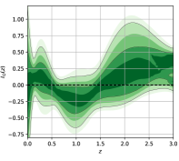
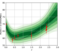
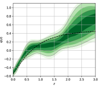
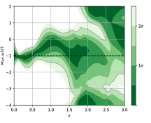
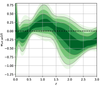
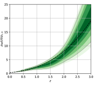
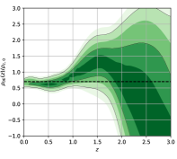
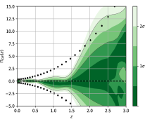
Figure 2: Functional posterior probability of the reconstruction by using a Gaussian Process and $w=-1$. The probability as normalised in each slice of constant $z$, with colour scale in confidence interval values (see color bar at the right). The 68% ($1\sigma$) and 95% ($2\sigma$) confidence intervals are plotted as black lines. From left to right in the upper part: the reescalation function $I_{Q}(z)$, the Hubble Parameter, the deceleration parameter and the effective EoS parameter for DE. In the lower part: the effective EoS parameter for DM, the density for DM and DE respectively and the dimensionless interaction kernel $\Pi_{\rm DE}$. The dashed black line corresponds to the standard $\Lambda$CDM values and the dotted line in the $\Pi_{\rm DE}(z)$ plot corresponds to the $\Omega_{\rm m}H(z)^{2}/H_{0}^{2}$ curve.

Once we have performed the reconstruction of $\Pi(z)$, we are able to extract some derived features, shown in Figs. 2 and 3. Here, we plot the functional posteriors for the quantities: $H(z)/(1+z)$ (corresponding to the expansion speed of the universe, i.e., $\dot{a}$ with $a$ being the scale factor), Solano’s dimensionless interaction function $I_{Q}(z)$, the deceleration parameter $q(z)$, the two effective EoS parameters ($w_{\rm eff,\rm DM}$ and $w_{\rm eff,\rm DE}$), and both energy densities ($\rho_{\rm DM}/\rho_{\rm c,0}$ and $\rho_{\rm DE}/\rho_{\rm c,0}$). Both figures present a similar structure in the results, but the case where the EoS parameter is free to vary (Fig. 3) is a bit more pronounced, hence we focus on this case. The general form of $\Pi(z)$, including its oscillatory behavior, is transferred to the derived functions. For instance, and as noted before, the presence of maxima in the interaction kernel may be able to explain the BAO data. This can be seen in the panel with $H(z)/(1+z)$, which contributes to alleviate the BAO tension created between low redshift (galaxies) and high (Ly-$\alpha$) data, explored in [151, 60]. The fact that the general form of $H(z)/(1+z)$ changed, causes a displacement of its minimum value which in turn moves the beginning of the acceleration epoch to lower values of redshift, i.e. $q(z)=0$ at $z\sim 0.5$ at 68% CL away from the $\Lambda$CDM value. The main differences of the $\Lambda$CDM and the reconstructed IDE are accentuated on the functional posterior of the re-escalation function $I_{Q}(z)$. Here we notice the existence of regions where the standard model remains outside the 68% CL (1-$\sigma$), which could motivate further studies of an interaction kernel with the presence of oscillations. The general tendency of this function also resembles a previously obtained result in [123] with regards to the predominant negative values at late times. The last reconstructed derived features are the effective equations of state parameters and the energy densities. The effective EoS parameter of the DE, at low redshift, resembles a Quintom-like behavior crossing the phantom-divide-line (PDL), viz., $w_{\Lambda}=-1$, multiple times; as studied in [68]. A primary characteristic of the effective EoS parameter is exhibiting a pole (viz., ${\lim_{z\to z_{\dagger}^{\pm}}w_{\rm DE}(z)=\pm\infty}$ with $z_{\dagger}$ being the singular point). As studied in previous works [72, 62, 119, 155] this is necessary when a transition to a negative energy density is present, and this can also be easily verifiable by looking at the DE density, $\rho_{\rm DE}/\rho_{\rm c,0}$, which allows a transition to negative values at about $z\sim 2.3$. As a consequence of the interacting mechanism, the DM effective EoS parameter also shows some oscillations, although statistically in agreement with $w_{\rm DM}=0$. Because the effective DM EoS parameter is a function of $Q(z)$ one finds that, if $Q(z)\neq 0$ then the DM would be no longer exhibit $\rho\propto a^{-3}$, i.e., no longer would behave like a fluid with a pressure identical to zero. This result is similar to the one obtained in [156], where the term used for a DM with a dynamic EoS parameter was named Generalized dark matter (GDM). On the other hand, its energy density shows a tendency towards smaller values than $\Lambda$CDM (dashed line) at low redshifts, a possible transition to null or negative values at $z\sim 2.3$ and then larger values at higher redshifts. This is a consequence of the changing direction in the energy transfer.

Table 2: Mean values, and standard deviations, for the parameters used throughout the reconstructions. For each model, the last two columns present the Bayes Factor, and the $-2\Delta\ln\mathcal{L_{\rm max}}\equiv-2\ln(\mathcal{L_{\rm max}}_{,\Lambda\text{CDM}}/\mathcal{L_{\rm max,}}_{i}$) for fitness comparison. The datasets used are BAO+H+SN. Here $-2\ln\mathcal{L_{\rm max}}_{,\Lambda\text{CDM}}=1429.7$, $\ln E_{\Lambda\text{CDM}}=-721.35(0.14)$.

Model	EoS parameter	$h$	$\Omega_{\rm m}$	$\ln B_{\Lambda\text{CDM},i}$	$-2\Delta\ln\mathcal{L_{\rm max}}$
$\Lambda$CDM	-1	0.683 (0.008)	0.306 (0.013)	0	0
$w$CDM	$w_{c}$	0.675 (0.022)	0.296 (0.016)	1.51 (0.18)	-2.73
CPL	$w_{0}+w_{a}(1-a)$	0.676 (0.023)	0.298 (0.019)	2.37 (0.19)	-2.81
SSIK	$w_{0}$	0.681 (0.025)	0.303 (0.027)	3.82 (0.21)	-3.12
$\Pi_{\rm DE}$ GP	-1	0.684 (0.027)	0.321 (0.032)	8.61 (0.21)	-3.89
	$w_{0}$	0.687 (0.027)	0.311 (0.024)	8.01 (0.21)	-4.22
$\Pi_{\rm DE}$ bins	-1	0.684 (0.025)	0.319 (0.027)	5.69 (0.22)	-3.88
	$w_{0}$	0.689 (0.027)	0.314 (0.025)	7.51 (0.22)	-3.92

Table 3: Constraints at 68% CL of the parameters for our model-independent reconstructions. The values for $\Pi_{4}$ are unconstrained for some of the cases, and for $\Pi_{5}$ for every case, which is expected given the lack of data in this redshift.

Model	$w_{0}$	$\Pi_{1}$	$\Pi_{2}$	$\Pi_{3}$	$\Pi_{4}$	$\Pi_{5}$
$\Pi_{\rm DE}$ GP	$-1$	$-0.01(0.26)$	$-0.26(0.36)$	$-0.29(1.04)$	$0.93(5.34)$	unconstr.
	$-0.81(0.16)$	$-0.78(0.71)$	$-0.16(0.39)$	$-0.22(1.14)$	$5.35(5.82)$	unconstr.
$\Pi_{\rm DE}$ bins	$-1$	$0.04(0.05)$	$-0.61(0.56)$	$0.54(3.16)$	unconstr.	unconstr.
	$-0.98(0.09)$	$0.02(0.06)$	$-0.43(0.76)$	$0.18(3.55)$	unconstr.	unconstr.

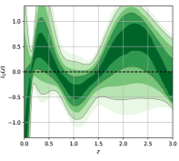
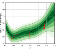
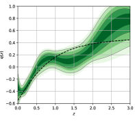
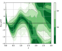
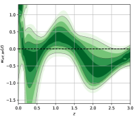
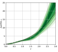
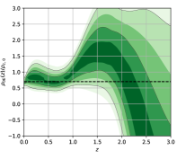
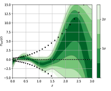
Figure 3: Functional posterior probability of the reconstruction by using a Gaussian Process and $w=w_{0}$. The probability as normalised in each slice of constant $z$, with colour scale in confidence interval values. The 68% ($1\sigma$) and 95% ($2\sigma$) confidence intervals are plotted as black lines. From left to right in the upper part: the reescalation function $I_{Q}(z)$, the Hubble Parameter, the deceleration parameter and the effective EoS parameter for DE. In the lower part: the effective EoS parameter for DM, the density for DM and DE respectively and the dimensionless interaction kernel $\Pi_{\rm DE}$. The dashed black line corresponds to the standard $\Lambda$CDM values and the dotted line in the $\Pi_{\rm DE}(z)$ plot corresponds to the $\Omega_{\rm m}H(z)^{2}/H_{0}^{2}$ curve.

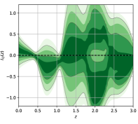
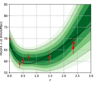
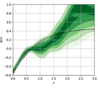
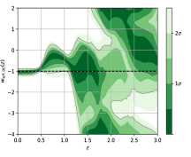
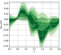
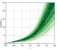
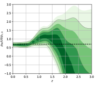
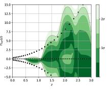
Figure 4: Functional posterior probability of the reconstruction by using a Binning scheme and $w=-1$. The probability as normalised in each slice of constant $z$, with colour scale in confidence interval values. The 68% ($1\sigma$) and 95% ($2\sigma$) confidence intervals are plotted as black lines. From left to right in the upper part: the reescalation function $I_{Q}(z)$, the Hubble Parameter, the deceleration parameter and the effective EoS parameter for DE. In the lower part: the effective EoS parameter for DM, the density for DM and DE respectively and the dimensionless interaction kernel $\Pi_{\rm DE}$. The dashed black line corresponds to the standard $\Lambda$CDM values and the dotted line in the $\Pi_{\rm DE}(z)$ plot corresponds to the $\Omega_{\rm m}H(z)^{2}/H_{0}^{2}$ curve.

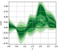
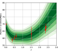
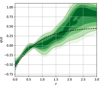
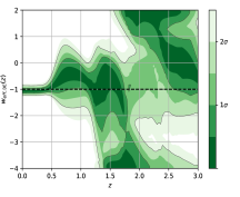
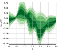
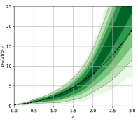
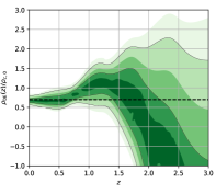
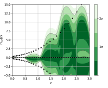
Figure 5: Functional posterior probability of the reconstruction by using a Binning scheme and $w=w_{0}$. The probability as normalised in each slice of constant $z$, with colour scale in confidence interval values. The 68% ($1\sigma$) and 95% ($2\sigma$) confidence intervals are plotted as black lines. From left to right in the upper part: the reescalation function $I_{Q}(z)$, the Hubble Parameter, the deceleration parameter and the effective EoS parameter for DE. In the lower part: the effective EoS parameter for DM, the density for DM and DE respectively and the dimensionless interaction kernel $\Pi_{\rm DE}$. The dashed black line corresponds to the standard $\Lambda$CDM values and the dotted line in the $\Pi_{\rm DE}(z)$ plot corresponds to the $\Omega_{\rm m}H(z)^{2}/H_{0}^{2}$ curve.

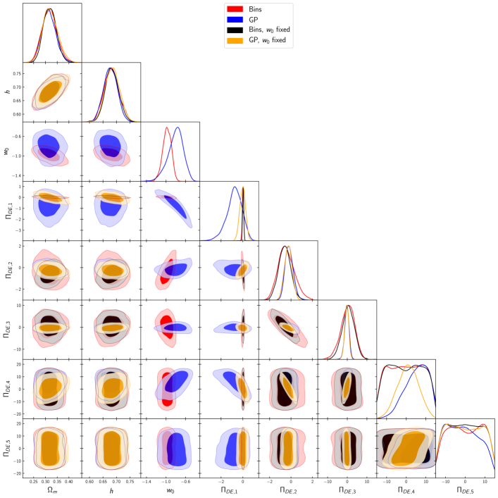
Figure 6: Triangle plot of every model-independent reconstruction. The parameter $w_{0}$ is only present in two of the reconstructions and it is correlated with $\Pi_{{\rm DE},1}$ when using a GP to perform the interpolation.

Next we present the results of the reconstruction using bins with Eq. 13 instead of GP. The functional posteriors can be seen in Fig. 4 ($w=-1$) and Fig. 5 ($w=w_{0}$). They look quite similar to the general features of the GP counterparts. When having $w=-1$ we obtain a $-2\Delta\ln\mathcal{L_{\rm max}}=-3.88$, and if the DE EoS parameter is allowed to vary we get $w_{0}=-0.98\pm 0.09$ and $-2\Delta\ln\mathcal{L_{\rm max}}=-3.92$ with respect to the $\Lambda$CDM scenario, improving the fit of the data and also performing slightly similar the reconstruction made with the GP interpolation. The results for this case also present oscillations around the null value of the interaction kernel $\Pi_{\rm DE}=0$ which, again, indicates more than one shift in the direction of energy density transfer. However, by using bins, the oscillations are noisier and thus more difficult to spot than in the one performed using GP; the results of the two cases, with fixed or varying EoS parameter, are very similar to each other. As far as the reconstructed derived features, we have a similar behavior to that found with GP. The re-escalation function $I_{Q}(z)$, for example presents some oscillatory-like behavior, that is less pronounced than the GP case, but lacks the first peak at redshift $z\sim 0.5$. The Hubble parameter presents a horizontal flat region (darker green). However, due to the larger confidence contours, it causes the existence of a region where the deceleration parameter equals zero, $z\sim 0.5-1.2$. Finally, the effective DE EoS parameter presents again a pole, but in this case closer to $z=2$, which indicates that the DE density, or $\rho_{\rm DE}(z)/\rho_{\rm c,0}$, is allowed to transit to negative values; and the effective DM EoS parameter shows deviations from zero at more than 1$\sigma$ level. These similar behaviors were expected as both model-independent reconstructions have similar degrees of freedom and the demeanor in which the nodes/bins are interpolated also have some visual similarities (as seen in Fig. 1 depending on the smoothness of the bins). However, it is crucial to emphasize here that while their similarities are noteworthy, their differences are of equal importance. We will discuss this point in more detail at the end of this section.

In Table 2 we have the mean values and standard deviations for our parameter estimation procedure. Every model-independent reconstruction, regardless of its improvement in the fit of the data, presents a worse Bayes’ Factor when compared to $\Lambda$CDM, because additional degrees of freedom are penalized by the Occam’s razor principle. In Fig. 6 we plot the 1D and 2D marginalized posteriors of the parameters corresponding to $\Pi(z)$ and in Table 3 we report their constraints at 68% CL, where the error is shown in parenthesis. The parameter $\Pi_{1}$, which is located in $z=0$ for GP, is clearly better constrained when taking $w=-1$, although its constraint is around $\Pi_{1}=0$, which indicates that, without a variable EoS parameter, it is pretty much forced to behave as $\Lambda$CDM at low redshifts.

When allowing variations on $w_{0}$, we note a separation from a $\Lambda$CDM-like behavior of around $1.5\sigma$ in $\Pi_{1}$ for GP. In contrast, when using bins this parameter is well constrained with or without a varying $w_{0}$. This happens because each bin spans a range ($\Delta z=0.6$ in this case) and, specifically the first bin, is fitting all the available data in $0<z<0.6$ with a single step function making it very constrained, unlike its GP counterpart which uses both $\Pi_{1}$ and $\Pi_{2}$ (interpolated in $0<z<0.75$). Another interesting observation is that the restriction in $\Pi_{1}$ is reflected in the posterior of $w_{0}$, allowing it to be higher than $-1$ and presenting a negative correlation with $\Pi_{1}$ when using GP. The parameter $\Pi_{3}$ on the other hand, appears to be more constrained with GP than with bins. We can also see from the marginalized 1D posteriors that the parameter $\Pi_{4}$ is loosely constrained when using GP but unconstrained with bins. This different behavior could be attributed to the slight correlation imposed by the GP method, but also when $w_{0}$ is allowed to vary we see it is correlated with $\Pi_{4}$, and at the same time $\Pi_{4}$ is correlated with $\Pi_{1}$ which is also constrained. $\Pi_{5}$ is completely unconstrained in all cases, but this was expected given the lack of data in this region ($z>2.4$). Despite the significant findings presented above, it should be noted that the standard $\Lambda$CDM model still remains a viable option within the 2$\sigma$ confidence level, which means that we cannot definitely exclude it with the data we used in this study, and we need additional and more precise data sets to be able to say anything solid about this possibility. Let us continue with a brief discussion of the differences and similarities between the findings from the two different reconstruction approaches we used. For instance, it can be easily seen that certain characteristics are more evident in the GP reconstruction than in the binning method. This discrepancy could be attributed to the inherent correlations existing within GP among nodes, a correlation that is subtly reflected in the confidence contours shown in Fig. 6. These correlations seem to favor the GP approach, which is evidenced by a better fit of this approach to the data as can be seen in Table 2. To reconcile these discrepancies among the approaches, a straightforward solution involves increasing the number of parameters, thereby achieving higher resolution. Nonetheless, this approach introduces the challenge of potential overfitting of specific characteristics and underfitting of others. To counterbalance this trade-off, we may need to incorporate a correlation function into the the binning method [157, 119], but the consideration of this is beyond the scope of the present work although it might be a promising direction for future investigations. It seems reasonable to conclude from this discussion that some of the observed features may be influenced by the chosen reconstruction method, but certain general characteristics persist regardless of the approach. These enduring traits include the oscillatory behavior at $1\sigma$, the asymptotic behavior of the effective EoS and the possibility of a transition to a negative DE density.

We conclude this section by commenting on one of the most interesting findings of our study, the possibility of the existence of a DE that can take negative density values at high redshifts (viz., for $z\gtrsim 2$), regardless of the approach used. Although this possibility may seem physically unexpected and challenging, it is not a new finding in our study and has been studied in the previous literature, especially recently, to address the cosmological tensions such as the $H_{0}$ and $S_{8}$ tensions; see, for instance, Refs. [60, 62, 63, 64, 66] considering models that suggest such a transition at $z\sim 2$ from their observational analysis and references therein for further reading. This type of DE behavior was also predicted in a model-independent manner in a recent study [119] that directly reconstructed the DE density. Our findings here present a noteworthy distinction with this recent study, as in the current study we achieved a similar behavior by incorporating an interacting dark sector (dark matter+dark energy) instead of employing a direct reconstruction of the DE interacting only gravitationally. This observation holds significance as it indicates that the data sets consistently favor (or at the very least allow for) a negative DE density for $z\gtrsim 2$, irrespective of the method employed. This finding, combined with the model’s potential to address certain cosmological tensions (as extensively discussed in [63, 64]), emphasizes the notion that this model emerges as a promising alternative to the standard $\Lambda$CDM model.

VI Conclusions

Throughout this paper, we performed model-independent reconstructions of the interaction kernel between DM and DE by implementing an interpolation with both Gaussian Process and bins joined via hyperbolic tangents, using the SimpleMC code along with the Nested Sampling algorithm. The main results showed that particular features, such as oscillations are present, but they remain still statistically consistent with the $\Lambda$CDM model. By using these reconstructions some derived functional posteriors were also obtained, which inherit the general characteristics of $\Pi(z)$. These oscillatory features can be more clearly observed through the reescalation function introduced in [128], and it is worth noting that similar shapes were also found in a model-independent reconstruction in [126]; (see also [158], suggesting that, in the relativistic cosmological models that deviate from $\Lambda$CDM, dark energies are expected to exhibit such behaviors for the consistency with CMB data). We noticed the Hubble parameter was slightly modified in order to alleviate the tension created between low and high redshift BAO data (reflected in the improvement of the fit) which also causes a shift, to later times, for the beginning of the acceleration epoch. When plotting the functional posterior of the DE effective EoS parameter we observed a quintom-like behavior at low redshift, with a preference zone of the $68\%$ confidence contour away from the $\Lambda$CDM. Additionally, we observe the presence of a pole at about $z\sim 2.3$ recovering a shape with an asymptote, proposed and studied in other works [72, 62, 119, 159, 160]. This particular shape is required when having a DE energy density that presents a transition from positive to negative energy density or vice versa. This transition is shown to be possible in the 68% contour of the derived DE energy density. Last but not least, an important implication of these reconstructions is seen with Eq. 8. We found a non negligible interaction kernel, thus the effective behavior of DM, at the largest scales, may not be described by a perfect pressure-less fluid but something around it.

Despite the positive outcomes observed in the fit of the data, we cannot ignore the Bayes’ Factors. As our model-independent method introduces several new parameters, it is expected to be in disadvantage when compared to the concordance model. To achieve improved results without disregarding our findings, it would be advisable to consider a new parameterization or a change in the basis with a considerably reduced number of parameters, that can take into account the new found features.