A New Forced Photometry Service for the Zwicky Transient Facility
Abstract
We describe the Zwicky Transient Facility (ZTF) Forced Photometry Service (ZFPS) as developed and maintained by the ZTF Science Data System Team at IPAC/Caltech. The service is open for public use following a subscription. The ZFPS has been operational since early 2020 and has been used to generate publication quality lightcurves for a myriad of science programs. The ZFPS has been recently upgraded to allow users to request forced-photometry lightcurves for up to 1500 sky positions per request in a single web-application submission. The underlying software has been recoded to take advantage of a parallel processing architecture with the most compute-intensive component rewritten in C and optimized for the available hardware. The ZTF processing cluster consists of 66 compute nodes, each hosting at least 16 physical cores. The compute nodes are generally idle following nightly real-time processing of the ZTF survey data and when other ad hoc processing tasks have been completed. The ZFPS and associated infrastructure at IPAC/Caltech therefore enable thousands of forced-photometry lightcurves to be generated along with a wealth of quality metrics to facilitate analyses and filtering of bad quality data prior to scientific use.
1 Introduction
The Zwicky Transient Facility (ZTF) is an optical time-domain survey that commenced operations in March 2018. ZTF uses the Palomar 48-inch Schmidt telescope and a custom-built wide-field camera providing a 47 deg2 field of view and 8 sec readout time, and can scan the entire northern visible sky at rates of 3760 square degrees/hour to median depths of and mag (AB, 5 in 30 sec). The design and implementation of the camera and observing system are described in Bellm et al. (2019). The ZTF Data System at IPAC/Caltech provides near-real-time reduction of the image data to identify moving and varying objects, and produces astrometrically and photometrically calibrated source catalogs as the survey proceeds (Masci et al., 2019). ZTF’s science objectives were presented in Graham et al. (2019).
The single-exposure source catalogs generated by the automated processing pipeline assume a fixed detection threshold along with filtering of other quality criteria following PSF-fit photometry (for details, see Masci et al., 2019). A consequence of this fixed-threshold approach is that only measurements of a source that satisfied the detection threshold (nominally 5) across a span of exposures are saved and catalogued. Sources that vary and intermittently fall below the threshold are missed, causing individual lightcurves constructed from the standard pipeline products to be highly incomplete and irregular as a function of observation epoch. Furthermore, the absence of measurements below the detection limit prevents single-epoch upper limits on a source’s location to be determined. A forced photometry service, customized for ZTF (the ZFPS) was implemented to circumvent these limitations.
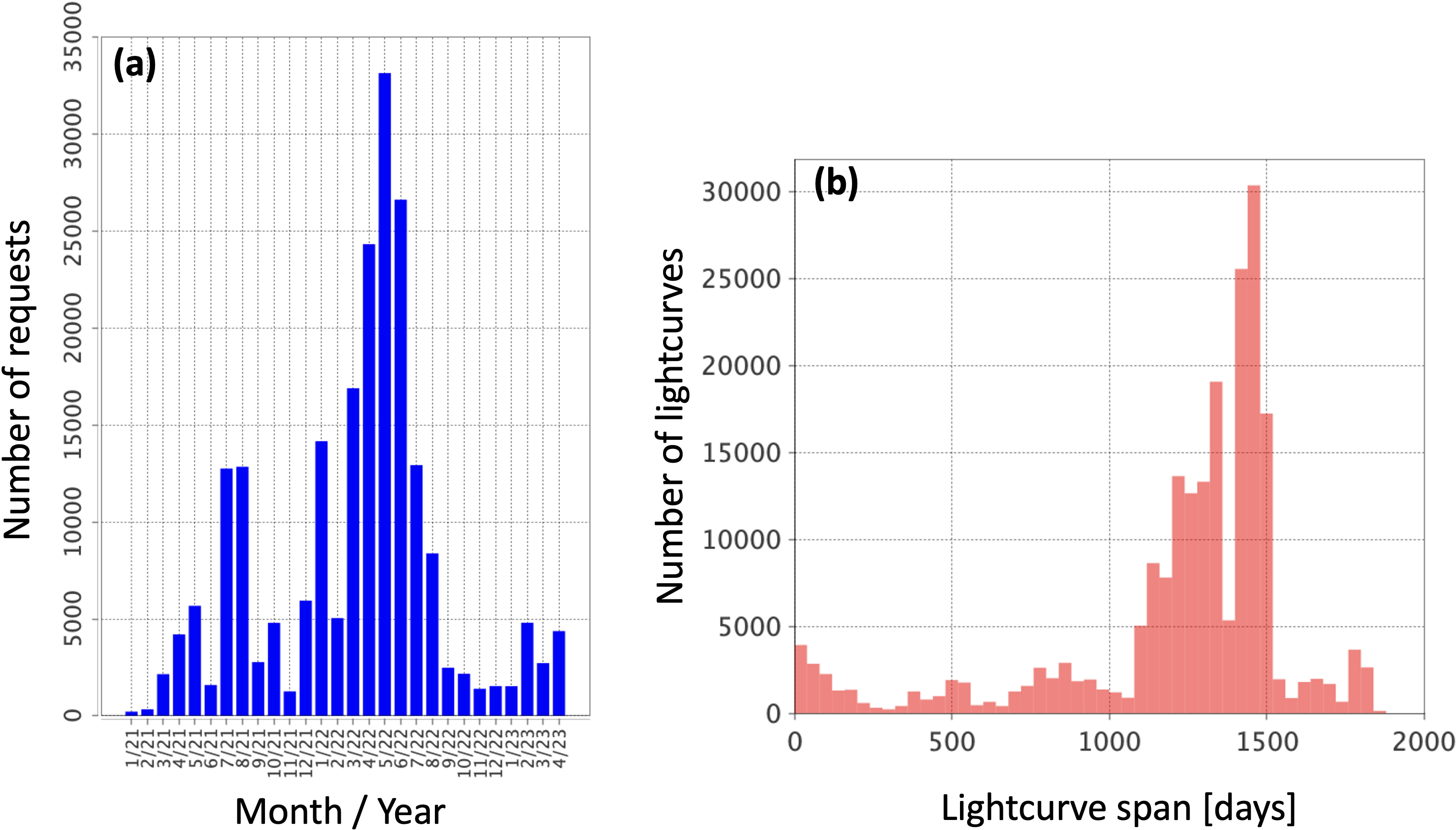
An early implementation of the ZFPS was based on accepting single source positions with timespans per request111https://irsa.ipac.caltech.edu/data/ZTF/docs/ztf_forced_photometry.pdf. Given the prodigious increase in the number of transient and variable source candidates from the ZTF survey requiring detailed lightcurves to facilitate classification, there was a demand to improve the processing throughput of the ZFPS. The new service can handle over 100 times more individual source requests than the initial version, where users can submit requests in a batch-like manner. Figure 1a summarizes the usage statistics of the service so far, going back to when requests were first logged into a database (January 2021). Figure 1b shows the distribution of lightcurve spans over all requests. The peak at days (approaching fours years) is due to requests to support studies of variability in Active Galactic Nuclei (AGN; e.g., Demianenko et al., 2022a, b). At this time, there are 256 subscribed users.
This write-up is primarily a user-guide to the new ZFPS. Section 3 describes how to submit forced photometry requests to operate specifically on difference images stored in the ZTF archive hosted by the NASA/IPAC Infrared Science Archive (IRSA)222https://irsa.ipac.caltech.edu/Missions/ztf.html. By “difference images”, we mean images constructed by subtracting a reference image (co-add) constructed from early ZTF survey image data from single-epoch science images. Use of difference images for forced photometry provides an enormous advantage over epochal science images due to the suppression of source confusion in crowded regions and complex backgrounds. Difference images are generated by IPAC’s ZTF real-time production pipeline and were described by Masci et al. (2019). Section 3.1 provides a performance benchmark to enable users to estimate the expected turnaround time following a submission. Instructions on how to retrieve lightcurve products following submission and processing are described in § 3.2. Recipes for generating publication-quality lightcurves from the raw output, as well as caveats, warnings, suggestions for improving their quality, and computing upper limits are described in § 6. A method for combining measurements in order to recover signals below the single-exposure sensitivity limit or place tighter constraints on non-detections is described in § 6.6. A checklist of all user instructions, including a recipe on how to analyze a ZFPS lightcurve is summarized in § 7. Acronyms are defined in Appendix C.
2 Overview of the ZFPS
The ZTF camera generates 64 CCD-quadrant images (also known as readout-channel images) per exposure, in one of three filters (, , and ), and located on one of the 1338 predefined science Fields that cover the northern sky visible from Mt. Palomar Observatory. To date, nearly one million science exposures have been acquired and 44% of these have products archived in IRSA. Eventually, all ZTF survey data products will reside in IRSA and be publicly available. The ZFPS will continue to be operational and integrated with the ZTF archive following completion of survey operations.
For a given sky position and time span, a forced-photometry lightcurve is generated for all ZTF camera filters and images according to user data-access privileges (for example, embargoed ZTF partnership data versus data that is now publicly accessible). Internally, the sky positions provided by different users are aggregated according to distinct predefined ZTF Field and CCD-quadrant locations on the sky. These are then processed together on the same compute node for maximal efficiency since the input positions are likely to be from the same images. This minimizes the I/O load for marshaling large numbers of difference images onto a given compute node.
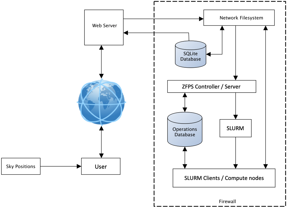
Figure 2 shows the ZFPS data flow along with its major hardware components. As mentioned earlier, the previous version of this service processed only one sky position per user submission. The new batch-like service described here represents a significant improvement in terms of the number of lightcurves that can be generated and delivered within any given period. The components and interfaces in Figure 2 are described in § 4.
3 User Instructions
Users will first need to register to use the forced-photometry service. All users who previously registered to use the initial version of the ZFPS are automatically enrolled and granted the same access privileges to the new batch-based service. A large portion of the ZTF data is public and available to everyone; students and post-doctoral scholars are encouraged to subscribe. New users are invited and can register by sending an e-mail to ztf@ipac.caltech.edu333This e-mail address can also be used for helpdesk questions. requesting access to the service. It is strongly advised that users who are affiliated with an academic institution provide their institutional e-mail address. Individuals should also indicate if they are a member of the ZTF Partnership or ZTF Project at Caltech. A confidential password (designated userpass below) is assigned to the registered e-mail and sent to the user upon enrollment.
Prior to submitting requests to the ZFPS (§ 3.1), it is advised you check your sky positions for accuracy (at least a few of them if you have multiple positions), in particular that they reflect what would be measured directly off IPAC’s astrometrically-calibrated images in the ZTF archive. It is advised that these positions be checked using epochal images where the signals of your targets are significant relative to the local noise. Positional biases due to definition of the astrometric reference system or from uncorrected drifts over time may exist. We advise that positions be specified in equatorial coordinates in the ICRF used to define the astrometric system of Gaia DR1, which is at epoch J2015 (Mignard et al., 2016) and is consistent with the ICRS to mas. This is the astrometric reference catalog used to astrometrically calibrate all ZTF image and source catalog products. Furthermore, coordinates defined on the J2000 (or the Earth Mean Equator 2000) system are within 20 mas of the ICRS (Kaplan, 2005). This is small enough to ignore when working with ZTF epochal images since the RMS error in the reconstructed astrometry per image is typically 60 mas per axis (Masci et al., 2019).
Users should also plan on requesting a sufficient number of future and/or historical epochs after/prior to the epoch or period defining the transient event or variability behavior of interest. An additional epochs is suggested. The purpose is to enable a possible baseline correction (§ 6.2) and/or uncertainty rescaling (§ 6.3). This will also allow the combining of single-epoch measurements in order to go deeper (§ 6.6). Additional future/historical epochs are usually unnecessary for continuous reoccurring (a)periodic variables.
3.1 Submitting Requests
The official URL of the ZFPS portal is
https://ztfweb.ipac.caltech.edu/batchfp.html
This webpage will contain periodic updates for users such as the status of the ZFPS, for example, scheduled maintenance and downtimes, or updates to the universal ZFPS username or password.
Requests are submitted to the ZFPS using a Python3 script. An example script is provided in Appendix A. Users can use this template script to construct their own submission scripts. The email and userpass provided to the registered user following the subscription process must be updated in the script. The universal ztffps account associated with the auth keyword in the HTTP-post-request statement of the script also has a password, dontgocrazy!. This password is different from the userpass. This password should not be updated unless a message was broadcast to the ZFPS information webpage above.
As a demonstration, the Python script in Appendix A was used to submit 12,825 sky positions from the ZTF Bright Transient Survey (BTS; Fremling et al., 2020; Perley et al., 2020), the largest flux-limited supernova survey to date.444https://sites.astro.caltech.edu/ztf/bts/bts.php As written, the script sent nine separate submissions (via a “for loop” at the bottom), each limited to no more than 1500 sky positions. This is currently the maximum size of a batch submission and it avoids the following error from being generated: “Error: 413 Request Entity Too Large”.
The Python script requires that sky positions be specified in equatorial coordinates, in decimal format (see § 3 for preferred astrometric reference system). These coordinates (RA Dec) are supplied in the hardcoded input file “List_of_RA_Dec.txt”, with one RA Dec position per line and a space between the RA and Dec values. The script also requires the observation start and end Julian Dates (JD) of the survey image epochs. For reference, the official ZTF-survey start date is 2018-03-17 00:00:00.0 UT ( days).
The maximum number of individual (distinct) target positions a user can have in the system is 15,000. The user will be notified via e-mail when this quota is exceeded, not more than once per day. Submitted sky positions above this limit will wait in a queue on the web server until the sky positions pending in the system have been processed to a number below the limit. Furthermore, safeguards are in place to prevent redundant requests from entering the system too frequently, in order to stave off possible malicious denial-of-service attacks. Users should refrain from submitting the same sky positions within a 90-day period. After 90 days, the same sky positions can be resubmitted and any newly acquired data will be used to augment the lightcurves.
For reference, the BTS set of lightcurves took days to compute in wall-clock terms. This processing occurred and continued during normal nightly survey operations as data from the observatory was received and processed at the nominal rate. Turnaround times for lightcurves will be faster during periods of bad weather, and slower when other data-processing tasks take priority.
3.2 Monitoring and Downloading Lightcurves
Users are notified via e-mail when their jobs are complete and lightcurve files are ready for download. For the BTS example request (§ 3.1), the user was notified via nine separate e-mails, one for each batch, or in other words, one for each execution of the Python requests.post function in the “for loop” of the submission script (Appendix A). Email notifications occur when all the sky positions in a specific batch request are completed and could thus be closed out.
Appendix B contains a script to check the completion of your submitted requests and if complete, returns a list of the URLs of your lightcurve file products for download. The returned list is formatted into wget ... lines that can then be executed in a terminal to download the lightcurve files. Users cannot query the filenames of lightcurves they do not own because the pathnames include a unique checksum that is not trivial to decipher.
The script in Appendix B queries a SQLite database that contains a 30-day sliding-window history of forced photometry requests. This database is remade at the top of each hour, and therefore jobs that finished within the hour will be updated with a lightcurve product filename and an exit code. The database queries executed by this tool can take several minutes to execute and return results. Requests older than 30 days will fall out of the SQLite database and will not be accessible to users through this tool. However, all lightcurve files and metadata in the operations database will be stored for the duration of the project, including those which are recomputed for the same sky positions.
4 Forced Photometry Methodology
At the heart of the ZFPS are photometry methods implemented in a C code, cforcepsfaper.c, which utilizes multi-threading for fast point-spread-function (PSF)-fit photometry, as well as aperture photometry. The code reads in a time-ordered list of difference images from the ZTF archive, for all filters (, , ), Fields and CCD-quadrants (or readout-channels) that cover the input sky positions. Only one of the available filters pertains to a single exposure. The code also reads a text file containing the ZFPS database request IDs, sky positions, and corresponding positions of the sky locations in each of the difference-image coordinate frames. Using this information, the code reads into memory the corresponding externally upsampled and renormalized PSF-image files (one per difference-image epoch), and a set of postage-stamp images generated from the difference images. These stamps have linear dimensions of native pixels and represent cutouts on the differences images centered on each respective sky position. Difference images and PSFs are initially generated by the real-time ZTF pipeline and are described in Masci et al. (2019).
The number of epochs and sky positions handled by the C code is limited by the available memory per compute node. The ZTF cluster consists of 66 compute nodes all of which are managed by the SLURM software.555https://slurm.schedmd.com/overview.html Each node has at least 16 CPU cores (with two threads admissible per core) and 125 GB of memory. All nodes are generally available for the ZFPS when not occupied with either regular nightly real-time processing, scheduled daily tasks and/or other ad hoc tasks. The C code is currently configured to process up to 15,000 epochs and 1,500 sky positions. The number of sky positions assigned to a given job is limited by the available memory per target compute node and number of parallel jobs running on that node. The number of simultaneous threads allowed by an execution instance of the C code is currently four.
The forced PSF-fit photometry method is simple in that it does not account for possible contamination by neighboring sources near the target position on a difference-image stamp. There is no attempt to model and subtract neighboring point sources or residuals from imperfect subtractions. Contamination due to source crowding (and/or residuals) is rare, but may be significant in the galactic plane. Possible overall contamination to the target signals sought can be accounted for when validating and rescaling the photometric uncertainties (see § 6.3).
Each epoch-dependent PSF is first upsampled using Gaussian interpolation as implemented by the Perl PDL map function. This is performed in the calling Perl program forcedphotometry_trim_cforcepsfaper_threads.pl. PSFs are upsampled by a factor of five per axis. Figure 3 shows an example PSF following upsampling.


The input () difference-image stamps are upsampled to match the upsampled PSF-image size, which is pixels. The upsampling of the difference-image stamps involves a simple subdivision of each input pixel into sub-pixels such that the original pixel values are preserved when the sub-pixel values are summed. The next step is to shift the upsampled difference-image stamp so that its center pixel coincides with the desired sky-position to an accuracy that’s limited by the upsampled pixel size (within 1/5 the linear size native pixel or arcsec per axis for ZTF image data). Difference-image pixels that fall off the output grid are trimmed and empty pixels are filled with zeroes following the realignment process.
At this stage, the number of bad pixels in the difference-image stamp is checked. If the fraction exceeds 50% of all pixels, no photometry is computed and the epoch is flagged with status = 55. If less than this fraction, the photometry will proceed, but it is provisionally flagged as a warning with status = 56. Note that photometric measurements on an epoch-by-epoch basis may be set to -99999 in the output lightcurve file. This indicates that a measurement could not be computed (see § 5).
The difference-image stamps are background-subtracted to account for local variations in background level (relative to the global zero-level expected in the input difference images from which the stamps were cut). The background, , is computed from the median of the values in the original data prior to upsampling after omitting values within a radius of 5 pixels from the center. The root-variance of the background pixel values, , is estimated from half the difference between the 84th and 16th percentiles (and also used in the uncertainty calculation described below). This estimate is a robust alternative to the standard deviation. No photometry is computed if there are fewer than 100 background pixels. In this case, the epoch is provisionally flagged with status = 54.
The upsampled PSF is converted into a weight map, , for use in the PSF-fit photometry step by scaling it by the inverse sum of the squares of normalized PSF pixel values. That is,
| (1) |
and
| (2) |
where is the normalized point-spread-function value at pixel and pixels.
The PSF-fitted flux, , is the summed pixel-by-pixel product of the weight map and the background-subtracted, upsampled, recentered difference-image stamp:
| (3) |
where is the recentered difference-image data at pixel , is the background computed for the stamp image as described above, is the weight-map contribution of the PSF at pixel (Equation 2), and is a correction factor (currently 0.89897 across all ZTF filters) to account for biases in the estimated flux. This correction was determined empirically by comparing simulated (truth input) fluxes to measured fluxes.
The 1- uncertainty in the PSF-fit flux estimate is given by
| (4) |
| (5) |
| (6) |
where is the effective detector electronic gain, in electrons (e-) per DN (digital number). The median value for in each filter across ZTF epochs is e-/DN. is the root variance of the background (see above).
The signal-to-noise ratio, SNR, is the PSF-fit flux (Equation 3) divided by its uncertainty (Equation 4):
| (7) |
and the reduced chi-squared statistic of the PSF fit, after accounting for independent degrees of freedom following upsampling, is
| (8) |
Concentric aperture photometry is also computed along with the PSF-fit photometry and included in the output lightcurve file. The aperture photometry estimates are generally noisier than the PSF-fitted estimates and serve as a crude quality check of the PSF-fitted estimates when many epochal measurements are compared. For a description of aperture photometry in general and its implementation in a stand-alone tool that is available for download, see Laher et al. (2012).
5 Exit and Warning Codes
Overall exit and warning codes from the ZFPS following execution of each sky-position request are provided on a per-epoch basis. These are given in the procstatus column of the output lightcurve file. These codes are defined in Table 1. Some of these codes were described in more detail in § 4. status = 52 in particular warns the user that the maximum of 10,000 target positions was exceeded. In this case, the user should submit another request with a later JD range in order to complete their lightcurves. The 10,000 limit is driven by the local disk space on a compute node and the number of concurrent forced-photometry jobs we are allowing per node.
| Code | Definition |
|---|---|
| 0 | Successful execution |
| 52 | 10,000 input-file limit reached |
| 54 | Insufficient number of background pixels |
| 55 | Too many bad pixels |
| 56 | Measurement impacted by bad or blank pixels |
| 57 | No reference-image-catalog source within 5″ |
| 58 | Reference image PSF-catalog does not exist |
| 61 | Sky position is off-image or too close to an edge |
| 62 | Requested start JD is before official survey start date |
| 63 | No records (epochs) returned by database query |
| 64 | Catastrophic error |
| 65 | Requested end JD is before official survey start date |
| 255 | Database or other error |
6 Analyzing a Lightcurve File
The lightcurve file produced by the ZFPS for a given sky position is a table formatted in ASCII text. The multi-column data records are space-delimited. At the beginning of each file is a header containing information about the request and a description of all the table columns. These lines are preceded by the # character. The data portion of the lightcurve file consists of observational metadata, quality metrics, and forced-photometry measurements for all epochs at the user’s allowed data-access level. Typically, this lightcurve file is no more than three or four megabytes in size. An example lightcurve filename is batchfp_req0000036025_lc.txt where the numeric string following _req is the unique database request ID.
The data table in a lightcurve file does not represent a standalone lightcurve that can be immediately plotted. It contains difference-image forced photometry measurements on the requested input position for the JD range covering all relevant ZTF Fields, CCD-quadrants, and filters (, , ), but only for difference-images that exist in the archive. Before constructing a lightcurve (§ 6.4 and § 6.5), the contents of the lightcurve file need to be analyzed such that rows (epochs) corresponding to a specific ZTF Field ID and filter of interest are stored, including any quality metrics to use for filtering of bad-quality data (see § 6.1). It’s possible that multiple Field IDs will cover the target position where each Field/CCD-quadrant combination will have used its own reference image for image-differencing. Each reference image may have been created from an entirely different set of historical observation epochs and therefore may introduce a different baseline for adjusting the resulting differential photometry (see § 6.2). This is primarily due to contamination from either a transient’s flux or other systematic residual in the reference image.
At minimum, the columns (as named in the lightcurve file) for constructing a forced PSF-fit-photometry differential lightcurve for a given Field, CCD-quadrant, and filter are: field, ccdid, qid, filter, jd, zpdiff, forcediffimflux, and forcediffimfluxunc. The combination of ccdid and qid refers to the specific CCD-quadrant of a given field. Due to variations in telescope pointing (and adjustments during the course of the survey), it is possible for a target position to fall on (or straddle) different CCD-quadrants of the same field. As mentioned above, it is important that forced-photometry measurements from the same field, ccdid, qid, and filter be analyzed (with all necessary corrections applied; see § 6.2 and § 6.3) prior to splicing them with measurements originating from other combinations of field, ccdid, and qid in the lightcurve file for the same filter.
6.1 Quality Filtering
Due to the automated nature of ZTF survey operations, a significant fraction of the data is non-photometric, that is, were acquired through intermittent cloud cover and/or were contaminated by moonlight, especially reflected from clouds. Intra-night changes in atmospheric transparency are inevitable and difficult to avoid or correct in near-realtime. This primarily affects the real-time photometric calibration (zero-point estimates zpdiff). In particular, spatial non-uniformities in photometric throughput on scales smaller than a CCD-quadrant (), however slight, severely impact difference-image quality and measurements performed thereon.
To account for possible bad photometric measurements, we advise omitting epochs that satisfy the three criteria below, based on a subset of the metrics provided in the lightcurve file. These were proven to be useful following analyses of large numbers of Type-Ia SN lightcurves (e.g., Yao et al., 2019).
-
•
Remove epochs with infobitssci . This is a 32-bit integer that encodes the status of processing and instrumental calibration steps for the science image. Each condition is assigned a specific bit and not all conditions are considered “fatal”. The value 33554432 () indicates in general, bad photometric calibration. A stricter criterion is to remove all epochs with infobitssci , but this is likely to remove measurements that could still be usable, albeit noisier.
-
•
Remove epochs with scisigpix DN. This metric is a robust estimate of the spatial noise-sigma per pixel in the science image computed via .
-
•
Remove epochs with ″. This represents the median seeing estimated from the FWHM of point sources extracted from the science image.
6.2 Baseline Correction
For a given field, ccdid, qid, and filter in the lightcurve file and following any filtering of bad data (§ 6.1), it is recommended you examine a plot of forcediffimflux [DN]) versus jd [day] to determine if there is any residual offset from the zero-baseline level. This residual offset refers to the level defined by either historical or future epochs in your lightcurve in flux [DN] space, where the measured signal (relative to the reference image) is stationary in time and fluctuating only due to the background noise. For example, if the reference image used to generate the difference images was contaminated by the transient’s flux, your baseline will be . The reference image may also be affected by some other systematic during its generation or calibration (including astrometric registration with the epochal science image), and therefore the resulting baseline could be .
Requesting a special time-range for regenerating a reference-image for the purpose of ensuring a zero baseline in the differential lightcurve is unnecessary. You will always need to check and correct for a non-zero baseline due to possible systematics. This will ensure the best accuracy following photometric calibration (see § 6.4). This correction is not necessary for (a)periodic variables that may fluctuate about a constant long-term flux-level. The reason is that even if the reference image was not a true (unbiased) time-average of all the input epochs (at random lightcurve phases), any residual baseline will need to be retained when converting the differential fluxes to direct (total) fluxes using the reference-image source catalog flux (see § 6.5).
The baseline correction needs to use a sufficient number of future and/or historical flux measurements. We suggest epochs. The more the better since measurements may be affected by stochastic effects, e.g., low transparency (intermittent cloud cover) and/or moon glow. Before submitting a ZFPS request, it is recommended you obtain some knowledge of the behavior of your transient or variability of interest (e.g., timescale) and include a sufficient number of epochs before and/or after its suspected duration.
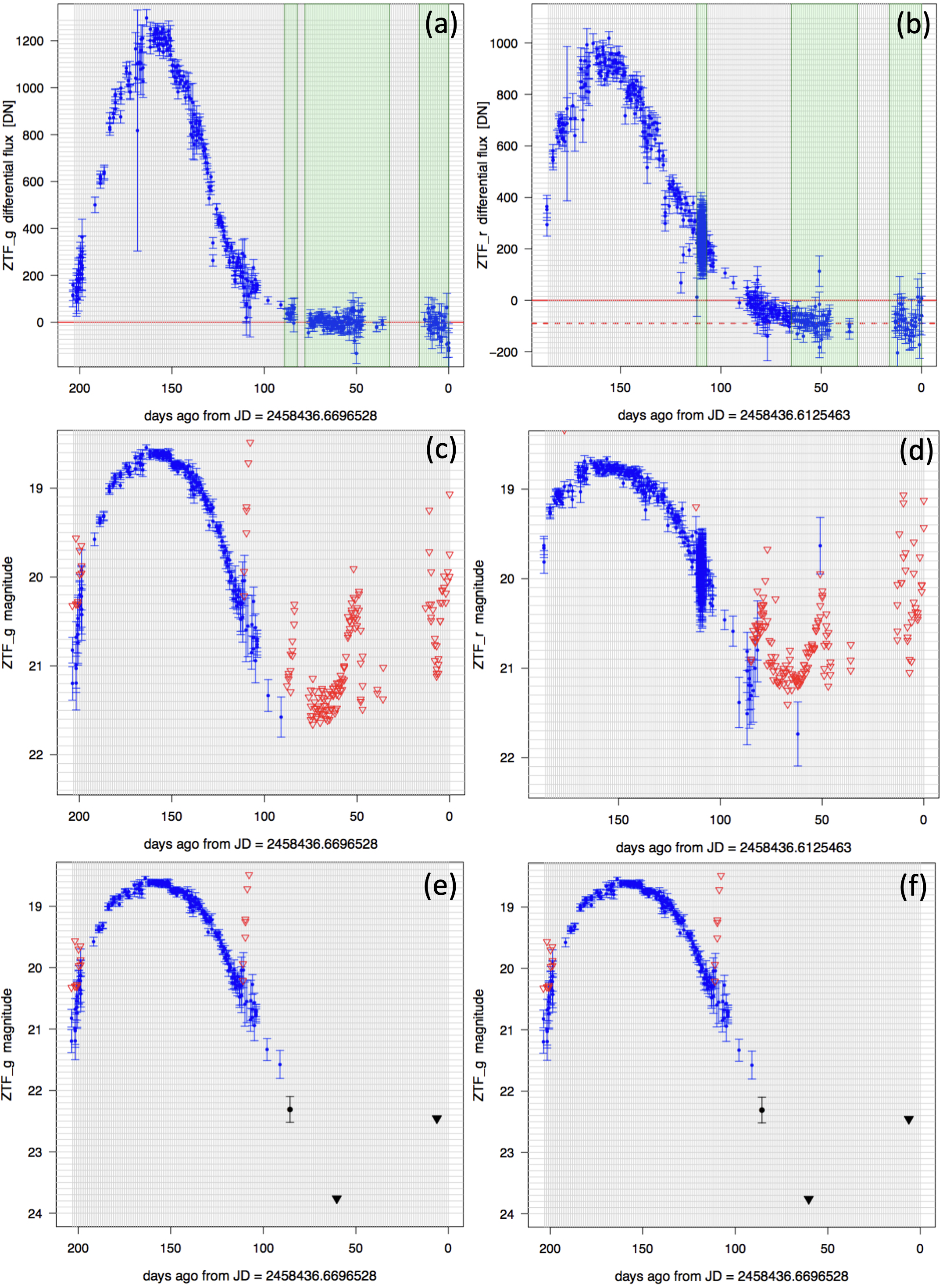
Figure 4 shows various lightcurves of the Type-I supernova SN 2018bym (Lunnan et al., 2020). Flux versus time plots in the and filters are shown in panels (a) and (b) respectively. The -filter plot shows a future baseline level of approximately –90 DN (dashed red line), as inferred from the differential fluxes at days where the supernova signal reaches quiescence. In practice, we recommend performing a trimmed-average or median of the measurements in this “stationary period” as guided by a visual examination of the flux lightcurve. Following an estimate of the baseline level, you will need to subtract this from all the differential flux measurements (forcediffimflux) before converting them to calibrated magnitudes or upper limits (see § 6.4).
6.3 Validating Flux-Uncertainty Estimates
Despite efforts to ensure the 1- uncertainties in the PSF-fit fluxes (forcediffimfluxunc) are correct, it is advised to check that these are still plausible, or at least consistent with the photometric repeatability expected at a given magnitude for the given filter and possibly sky location (field), i.e., in the frequentist sense.
The measurement uncertainties are based on propagating a semi-empirical model of the statistical (random) noise expected in the detector pixels through the difference- (and reference-) image pipelines. This model does not account for possible systematics, for example, errors in PSF estimates (such as variation over a CCD-quadrant), photometric calibration zero-points, flat-fielding errors, or astrometric calibration residuals, which will impact PSF-placement.
First, we advise checking the distribution of the PSF-fit reduced (forcediffimchisq) values for a given field and filter, following any quality filtering (§ 6.1). This can also be examined as a function of flux (forcediffimflux). The average (or some robust equivalent) of the forcediffimchisq values should be . If not, you should multiply the raw forcediffimfluxunc values by where the angled brackets denote average. Any flux-dependent forcediffimchisq could mean the [e-/DN] gain-factor for estimating the Poisson-noise component is not properly tuned or the PSF shape and hence flux-scaling is not correct. Ensuring only means the pixel uncertainties are consistent, in a statistical sense, with the PSF-fit residuals per epoch. It will not catch and correct for other possible systematics across the epochs (see below).
Following the forcediffimchisq check and possible rescaling, you can stop here or continue with another check to account for possible temporal systematics. This can be done by computing a robust RMS (e.g., via ) in the signal-to-noise (S/N) ratios (i.e., values) of the stationary-flux epochs that were used to infer your baseline level (§ 6.2). These ratios would be computed following any baseline correction to the forcediffimflux values and any prior scaling of the forcediffimfluxunc. If the uncertainties are plausible, this RMS should be . If not, the forcediffimfluxunc values can be multiplied by this RMS value. This will ensure the resulting distribution in S/N will have zero mean and unit variance. However, beware of epochs with bad data. This assumes the noise is approximately stationary during the historical/future epochs and they sample, to first order, the same underlying background and conditions as in epochs where the transient signal was detected.
The above RMS{S/N} check alone will not validate the Poisson-noise component in epochs when the transient has a high signal-to-noise ratio. A final (but still somewhat coarse) check for validating specifically the Poisson-noise-dominated regime can be performed by comparing against plots of prior-calibrated photometric-repeatability (stack-RMS) versus magnitude (e.g., see Figure 9 in Masci et al., 2019). This analysis will require you to first perform forced photometry on “non-variable” field stars covering flux ranges of interest, compute stack-RMS dispersions, then convert the fluxes and RMS values to calibrated magnitudes (see § 6.4 or § 6.5). It’s important to note that estimates of prior photometric uncertainties inferred in this manner will be field (sky location) dependent.
6.4 Converting Differential Fluxes to Calibrated Magnitudes
It is assumed the differential fluxes (forcediffimflux) have been corrected for any non-zero baseline (§ 6.2) and that flux uncertainties (forcediffimfluxunc) have been validated and possibly rescaled to conform to expectations (see § 6.3). If the uncertainties are overestimated or underestimated, the significance levels and hence derived upper limits will be incorrect. That is, “5-sigma” only has meaning if “sigma” is correct, and it captures all noise sources that may have corrupted the measurements.
The pseudo-code for obtaining calibrated magnitudes is below. It uses the following two parameters:
SNT = signal-to-noise threshold for declaring a flux measurement a ‘‘non-detection’’ so it
      can be assigned an upper-limit.
SNU = actual signal-to-noise ratio to use when computing a ‘‘SNU-sigma’’ upper-limit.
We recommend SNT and SNU . For details on why these were picked, see:
http://web.ipac.caltech.edu/staff/fmasci/home/mystats/UpperLimits_FM2011.pdfif ( forcediffimflux / forcediffimfluxunc ) > SNT: # We have a "confident" detection; compute and plot mag with error bar: mag = zpdiff - 2.5 * log10( forcediffimflux ) sigma_mag = 1.0857 * forcediffimfluxunc / forcediffimflux else: # Compute flux upper limit and plot as arrow or triangle: mag = zpdiff - 2.5 * log10( SNU * forcediffimfluxunc )
Lightcurves of SN 2018bym in the and filters converted to magnitudes using the above construction are shown in panels (c) and (d) of Figure 4.
6.5 Total Fluxes for Variable Sources and Conversion to Calibrated Magnitudes
Transients are generally defined as sudden events where signal suddenly appears out of the noise and then disappears. The goal is to analyze the energy released during the explosive (or perhaps implosive) phase, above or below some preexisting signal or background. For continuous (a)periodic variables or transients associated with pre-quiescent sources with detectable signal, one may want to characterize the total signal versus time (i.e., stationary pre-existing signal plus differential flux component). Here, an estimate is needed of the source flux from the reference image that was used to generate the difference-images on which the forced photometry was performed.
Photometry and quality metrics for the nearest reference-image source are given in the lightcurve file by columns prefixed with nearestref... These metrics are from the archived reference-image PSF-fit photometry source catalog. You will first need to threshold on the dnearestrefsrc value to ensure a reference source exists (was extracted) on or close-enough to your target position. We recommend ″. The nearestrefchi and nearestrefsharp metrics indicate whether the reference source is extended or PSF-like. If significantly extended, the PSF-fit photometry of the nearest reference-image source (nearestrefmag) will be erroneous. You will need to ensure the reference-image extraction is consistent with a point source.
Below are the steps for obtaining a “total flux” photometric light curve in calibrated magnitudes, modulated by variations inferred from differential photometry.
-
1.
Compute the reference source flux and its uncertainty on the same calibration (zero-point) as the differential flux at each epoch:
nearestrefflux = 10**[ 0.4 * ( zpdiff - nearestrefmag ) ]
nearestreffluxunc = nearestrefmagunc * nearestrefflux / 1.0857
where zpdiff, nearestrefmag, and nearestrefmagunc are given in the lightcurve-file data table.
-
2.
Compute the total flux, its uncertainty, and signal-to-noise ratio at each epoch:
Flux_tot = forcediffimflux + nearestrefflux
Fluxunc_tot = sqrt[ ( forcediffimfluxunc * forcediffimfluxunc
                    - nearestreffluxunc * nearestreffluxunc ) ]
SNR_tot = Flux_tot / Fluxunc_tot
The negative sign in the square-root follows from the (implicit) assumption that the reference source flux was measured from the same reference image used to generate the “science – reference” differential flux. Hence, the noise is anti-correlated. If this is not true or if the argument in the square-root is for whatever reason, we suggest adding the variances instead. This will be a conservative estimate.
-
3.
Using the outputs from item 2 and the SNT, SNU parameters defined in § 6.4, here is the pseudo-code for generating a “total-flux” photometric lightcurve:
if SNR_tot > SNT:
    # We have a "confident" detection; compute and plot mag with error bar:
    mag = zpdiff - 2.5 * log10( Flux_tot )
    sigma_mag = 1.0857 / SNR_tot
else:
    # Compute flux upper limit and plot as arrow or triangle:
    mag = zpdiff - 2.5 * log10( SNU * Fluxunc_tot )
This logic reduces to the differential-lightcurve generation logic in § 6.4 when and .
The above construction to compute calibrated magnitudes assumes the source of interest has zero color in the Pan-STARRS1 photometric system ( for - and -flux measurements; for -flux measurements). If you have prior information on the color or spectrum of your source in these bandpasses across epochs, the magnitude computations above can include the additive term: ) for and measurements, or ) for -filter measurements, where clrcoeff is a data column in the lightcurve file.
6.6 Going Deeper: combining single-epoch measurements
To make your lightcurve measurements more statistically significant and/or make upper-limit estimates tighter, you can attempt to combine the flux measurements within carefully selected time-windows using some optimal method. Before proceeding, it is assumed your single-epoch differential fluxes have been corrected for any non-zero baseline (in the case of transients; see § 6.2) and uncertainties have been validated and rescaled if necessary (see § 6.3).
In order to improve SNR from combining measurements, the important assumption is that the individual measurement errors be uncorrelated. This is generally true when the individual measurements on a target’s position are background (hence photon and/or read noise) dominated. In the case of image differencing however, systematics from imperfect subtractions from e.g., inaccurate PSF-matching, astrometric registration, and/or photometric-gain matching will dominate and persist beyond some limit where improvements stop. This limit is difficult to determine without use of prior information or constraints on your transient’s temporal behavior. For the most part however, the ZTF single epoch difference-image measurements are photon and/or read-noise dominated and some improvement in SNR is always possible by combining up to several tens of epochs before systematics will limit further improvement.
Before combining measurements, you will first need to place the fluxes on the same (fiducial) photometric zeropoint (call this ). You can pick any value for . A value that’s close to the epoch-dependent zeropoints ( values, where is an index over the values) will suffice. You will then rescale the corrected fluxes (forceddiffimflux) and uncertainties (forceddiffimfluxunc) as follows:
| (9) |
| (10) |
One method for combining the measurements is to assume the underlying source signal is stationary within a time-window and collapse the rescaled single-epoch fluxes () therein using an inverse-variance weighted average:
| (11) |
where
| (12) |
The uncertainty in is:
| (13) |
Equation 13 is effectively if one assumes the windowed single-epoch flux measurements have approximately the same uncertainty equal to some constant value or RMS. Therefore, the improvement in signal-to-noise ratio assuming uncorrelated measurements is no more than a factor of (however beware of systematic errors; see above). The important assumption is that the underlying source signal is constant within the window. It may appear constant within measurement error, but when many measurements are available, you can attempt to bin them in various ways to tease out possible hidden trends in the signal. A moving (weighted) average may also work, using a properly tuned window size. There is also a large collection of methods on local-polynomial regression fitting (e.g., Buja et al., 1989; Ledolter, 2008).
You can also attempt to collapse the measurements within windows by fitting a prior model of flux versus time, i.e., if you have prior (or contextual) knowledge from other data sources. The advantages of combining measurements in source-space across epochs as opposed to co-adding entire images in time-ordered slices are: (i) speed and (ii) greater flexibility when weighting and combining the data.
Having computed the window-collapsed fluxes (), you can now convert them to calibrated magnitudes with upper limits using the formalism in § 6.4 (for transients) or § 6.5 (for “total” photometry on re-occurring variable sources). The only difference is that you will need to use the value assumed when rescaling the input fluxes (see above). Panels (a) and (b) in Figure 4 show example windows (shaded green) where the single-epoch flux measurements were combined using a weighted average (Equations 11 and 13). The resulting calibrated measurements in the and filters with upper limits are shown in panels (e) and (f) of Figure 4.
7 Summary and Checklist
We have described the recently upgraded ZFPS, which now supports the submission of batch requests directly from a Python script. Instructions and guidelines for analyzing and generating photometrically-calibrated, publication-quality lightcurves were also presented. Below is a checklist with references to sections containing further details.
- 1.
-
2.
Consult the ZFPS information page: https://ztfweb.ipac.caltech.edu/batchfp.html for important updates relating to the service (§ 3.1).
- 3.
-
4.
You will be notified by email when your jobs are complete and lightcurve files are ready for download. You can monitor the status of your request by modifying and uploading the example script in Appendix B. Follow the steps therein to retrieve your lightcurve files when the script returns the wget ... lines. Also see details in § 3.2.
-
5.
To extract a lightcurve from a downloaded lightcurve file for a target position and given filter (= , , or ), ensure that only rows with the same values of field, ccdid, qid, and filter are extracted, as discussed in § 6. At minimum, store the following corresponding quantities and quality metrics: jd, zpdiff, forcediffimflux, forcediffimfluxunc, infobitssci, scisigpix, and sciinpseeing.
-
6.
Remove bad-quality measurements from the records stored in the previous step by thresholding on infobitssci, scisigpix, and sciinpseeing using the suggested thresholds in § 6.1.
-
7.
Examine a plot of forcediffimflux vs jd and perform a baseline correction if necessary as described in § 6.2. A baseline correction will not be necessary for the differential-flux lightcurves of (a)periodic variables for which you plan to convert to “total flux” lightcurves later (§ 6.5; see also step 10 below).
-
8.
Check whether the flux uncertainties (forcediffimfluxunc) are plausible using the tests suggested in § 6.3. If not, compute correction factors and correct the forcediffimfluxunc values.
-
9.
If your lightcurve corresponds to transient behaviour over some finite timespan, convert the differential fluxes to calibrated magnitudes or upper limits following the recipe in § 6.4.
-
10.
If you are interested in recovering the total signal versus time for a lightcurve and wish to convert total instrumental fluxes to calibrated magnitudes, follow the recipe in § 6.5.
-
11.
If you are interested in combining single-epoch measurements in order to improve SNR or place tighter upper limits on non-detections, follow the suggestions in § 6.6.
Based on observations obtained with the Samuel Oschin Telescope 48-inch and the 60-inch Telescope at the Palomar Observatory as part of the Zwicky Transient Facility project. ZTF is supported by the National Science Foundation under Grants No. AST-1440341 and AST-2034437 and a collaboration including current partners Caltech, IPAC, the Weizmann Institute of Science, the Oskar Klein Center at Stockholm University, the University of Maryland, Deutsches Elektronen-Synchrotron and Humboldt University, the TANGO Consortium of Taiwan, the University of Wisconsin at Milwaukee, Trinity College Dublin, Lawrence Livermore National Laboratories, IN2P3, University of Warwick, Ruhr University Bochum, Northwestern University and former partners the University of Washington, Los Alamos National Laboratories, and Lawrence Berkeley National Laboratories. Operations are conducted by COO, IPAC, and UW. The ZTF forced-photometry service was funded under the Heising-Simons Foundation grant #12540303 (PI: M. J. Graham).
References
- Bellm et al. (2019) Bellm, E. C., Kulkarni, S. R., Graham, M. J., et al. 2019, PASP, 131, 018002, doi: 10.1088/1538-3873/aaecbe
- Buja et al. (1989) Buja, A., Hastie, T., & Tibshirani, R. 1989, The Annals of Statistics, 17, 453. http://www.jstor.org/stable/2241560
- Demianenko et al. (2022a) Demianenko, M., Grishin, K., Toptun, V., et al. 2022a, in Astronomy at the Epoch of Multimessenger Studies, 359–361, doi: 10.51194/VAK2021.2022.1.1.144
- Demianenko et al. (2022b) Demianenko, M., Grishin, K., Toptun, V., et al. 2022b, arXiv e-prints, arXiv:2201.03712, doi: 10.48550/arXiv.2201.03712
- Fremling et al. (2020) Fremling, C., Miller, A. A., Sharma, Y., et al. 2020, ApJ, 895, 32, doi: 10.3847/1538-4357/ab8943
- Graham et al. (2019) Graham, M. J., Kulkarni, S. R., Bellm, E. C., et al. 2019, PASP, 131, 078001, doi: 10.1088/1538-3873/ab006c
- Kaplan (2005) Kaplan, G. H. 2005, U.S. Naval Observatory Circulars, 179, doi: 10.48550/arXiv.astro-ph/0602086
- Laher et al. (2012) Laher, R. R., Gorjian, V., Rebull, L. M., et al. 2012, PASP, 124, 737, doi: 10.1086/666883
- Ledolter (2008) Ledolter, J. 2008, Communications in Statistics - Theory and Methods, 37, 959, doi: 10.1080/03610920701693843
- Lunnan et al. (2020) Lunnan, R., Yan, L., Perley, D. A., et al. 2020, The Astrophysical Journal, 901, 61, doi: 10.3847/1538-4357/abaeec
- Masci et al. (2019) Masci, F. J., Laher, R. R., Rusholme, B., et al. 2019, PASP, 131, 018003, doi: 10.1088/1538-3873/aae8ac
- Mignard et al. (2016) Mignard, F., Klioner, S., Lindegren, L., et al. 2016, A&A, 595, A5, doi: 10.1051/0004-6361/201629534
- Perley et al. (2020) Perley, D. A., Fremling, C., Sollerman, J., et al. 2020, ApJ, 904, 35, doi: 10.3847/1538-4357/abbd98
- Yao et al. (2019) Yao, Y., Miller, A. A., Kulkarni, S. R., et al. 2019, ApJ, 886, 152, doi: 10.3847/1538-4357/ab4cf5
Appendix A Submission Script Example
Below is an example script for submitting requests to the ZFPS, as described in § 3.1. Instructions are as follows:
-
1.
Ensure you have a version of Python3 installed (preferably version ). Also ensure the requests and json Python packages are installed.
-
2.
Copy and paste the lines that fall between the ‘‘’’ lines into a file named e.g., zfps_submit.py.
-
3.
Make this file an executable script. On a Linux/Unix operating system, this is the command: “chmod +x zfps_submit.py”.
-
4.
Update the JD range of interest. These are the jds and jde values in the script.
-
5.
Supply your email and userpass where indicated inside the script.
-
6.
Prepare a file containing a list of RA Dec positions in decimal degrees; one per line where the RA Dec are space-separated. This file is named “List_of_RA_Dec.txt” in the script.
-
7.
Execute the script to submit your batch request. On a Linux/Unix operating system, you would execute this at the command-prompt as “./zfps_submit.py”.
>>>>>>>>>>>>>>>>>>>>>>>>>>>>>>>>>>>>>>>>>>>>>>>>>>>>>>>>>>>>>>>>>>>
#!/usr/bin/env python3

import requests
import json

# Script name: zfps_submit.py

def submit_post(ra_list,dec_list):

    ra = json.dumps(ra_list)
    print(ra)
    dec = json.dumps(dec_list)
    print(dec)

    jds = 2458216.1234            # start JD for all input target positions.
    jdstart = json.dumps(jds)
    print(jdstart)

    jde = 2458450.0253            # end JD for all input target positions.
    jdend = json.dumps(jde)
    print(jdend)

    email = ’joeastronomer@caltech.edu’       # email you subscribed with.
    userpass = ’asdf123’                      # password that was issued to you.

    payload = {’ra’: ra, ’dec’: dec,
               ’jdstart’: jdstart, ’jdend’: jdend,
               ’email’: email, ’userpass’: userpass}

    # fixed IP address/URL where requests are submitted:
    url = ’https://ztfweb.ipac.caltech.edu/cgi-bin/batchfp.py/submit’

    r = requests.post(url,auth=(’ztffps’, ’dontgocrazy!’), data=payload)
    print("Status_code=",r.status_code)

#--------------------------------------------------
# Main calling program. Ensure "List_of_RA_Dec.txt"
# contains your RA Dec positions.

with open(’List_of_RA_Dec.txt’) as f:
    lines = f.readlines()
f.close()

print("Number of (ra,dec) pairs =", len(lines))

ralist = []
declist = []
i = 0
for line in lines:
    x = line.split()
    radbl = float(x[0])
    decdbl = float(x[1])

    raval = float(’%.7f’%(radbl))
    decval = float(’%.7f’%(decdbl))

    ralist.append(raval)
    declist.append(decval)

    i = i + 1
    rem = i % 1500    # Limit submission to 1500 sky positions.

    if rem == 0:
        submit_post(ralist,declist)
        ralist = []
        declist = []

if len(ralist) > 0:
    submit_post(ralist,declist)

exit(0)
>>>>>>>>>>>>>>>>>>>>>>>>>>>>>>>>>>>>>>>>>>>>>>>>>>>>>>>>>>>>>>>>>>>
Appendix B Job-Status Checking Script
Below is a script to check the completion of your submitted requests and if complete, returns a list of the URLs of your lightcurve file products for download as described in § 3.2. Instructions are as follows:
-
1.
Ensure you have a version of Python3 installed (preferably version ). Also ensure the requests and re Python packages are installed.
-
2.
Copy and paste the lines that fall between the ‘‘’’ lines into a file named e.g., check_status.py.
-
3.
Make this file an executable script. On a Linux/Unix operating system, this is the command: “chmod +x check_status.py”.
-
4.
Supply your email and userpass where indicated inside the script.
-
5.
If you are interested in the status of recently subitted jobs, ensure ’option’: in the script is set to ’All recent jobs’ (as currently indicated). If you are interested in checking for pending jobs, ensure ’option’: is set to ’Pending jobs’.
-
6.
Execute the script. On a Linux/Unix operating system, you would execute this at the command-prompt as “./check_status.py”.
Following execution, the script will either return a message such as Jobs either queued ..., or if complete, an actual listing of the URLs of the lightcurve files formatted into wget ... lines. These lines can be pasted and executed in a terminal window to download the lightcurve files. Below is an example output following completion of a request consisting of four sky positions. The “” are not part of the output; they are used here for splitting the long output lines.
./check_status.py
Script executed normally and queried the ZTF Batch Forced Photometry database.

wget --http-user=ztffps --http-passwd=dontgocrazy! -O  batchfp_req0000043161_lc.txt \
     "https://ztfweb.ipac.caltech.edu/ztf/ops/forcedphot/lc/batchfp/br000001-000100/32/\
     3f30e9eb728027c210739d20151911be/batchfp_req0000043161_lc.txt"
wget --http-user=ztffps --http-passwd=dontgocrazy! -O  batchfp_req0000043162_lc.txt \
     "https://ztfweb.ipac.caltech.edu/ztf/ops/forcedphot/lc/batchfp/br000001-000100/32/\
     3f30e9eb728027c210739d20151911be/batchfp_req0000043162_lc.txt"
wget --http-user=ztffps --http-passwd=dontgocrazy! -O  batchfp_req0000043163_lc.txt \
     "https://ztfweb.ipac.caltech.edu/ztf/ops/forcedphot/lc/batchfp/br000001-000100/33/\
     dc0d134536adc64b54df088eae99bd78/batchfp_req0000043163_lc.txt"
wget --http-user=ztffps --http-passwd=dontgocrazy! -O  batchfp_req0000043164_lc.txt \
     "https://ztfweb.ipac.caltech.edu/ztf/ops/forcedphot/lc/batchfp/br000001-000100/33/\
     dc0d134536adc64b54df088eae99bd78/batchfp_req0000043164_lc.txt"
Alternatively, the URL embedded in the script below, that is:
https://ztfweb.ipac.caltech.edu/cgi-bin/getBatchForcedPhotometryRequests.cgi
can be pasted into a browser in which case a webform will be displayed asking for your log-in details.
>>>>>>>>>>>>>>>>>>>>>>>>>>>>>>>>>>>>>>>>>>>>>>>>>>>>>>>>>>>>>>>>>>>
#!/usr/bin/env python3

import re
import requests

# Script name: check_status.py

settings = {’email’: ’joeastronomer@caltech.edu’,’userpass’: ’asdf123’,
            ’option’: ’All recent jobs’, ’action’: ’Query Database’}

r = requests.get(’https://ztfweb.ipac.caltech.edu/cgi-bin/’ +\
                 ’getBatchForcedPhotometryRequests.cgi’,
                 auth=(’ztffps’, ’dontgocrazy!’),params=settings)
#print(r.text)

if r.status_code == 200:
   print("Script executed normally and queried the ZTF Batch " +\
         "Forced Photometry database.\n")

   wget_prefix = ’wget --http-user=ztffps --http-passwd=dontgocrazy! -O ’
   wget_url = ’https://ztfweb.ipac.caltech.edu’
   wget_suffix = ’"’
   lightcurves = re.findall(r’/ztf/ops.+?lc.txt\b’,r.text)

   if lightcurves is not None:
      for lc in lightcurves:
         p = re.match(r’.+/(.+)’, lc)
         fileonly = p.group(1)
         print(wget_prefix + " " + fileonly + " \"" + wget_url + lc +\
               wget_suffix)
else:
   print("Status_code=",r.status_code,"; Jobs either queued or" +\
         "abnormal execution.")
>>>>>>>>>>>>>>>>>>>>>>>>>>>>>>>>>>>>>>>>>>>>>>>>>>>>>>>>>>>>>>>>>>>
Appendix C Acronyms
| AGN | Active Galactic Nuclei |
| ASCII | American Standard Code for Information Interchange |
| BTS | Bright Transient Survey |
| CCD | Charge Coupled Device |
| COO | Caltech Optical Observatories |
| CPU | Central Processing Unit |
| Dec | Declination |
| DN | Digital Number |
| DR | Data Release |
| FITS | Flexible Image Transport System |
| FWHM | Full Width at Half Maximum |
| HTTP | Hypertext Transfer Protocol |
| ICRF | International Celestial Reference Frame |
| ICRS | International Celestial Reference System |
| ID | Identifier |
| IN2P3 | L’Institut national de physique nucléaire et de physique des particules |
| IO | Input/Output |
| IRSA | NASA/IPAC Infrared Science Archive |
| JD | Julian Date |
| mas | Milli-arcseconds |
| NASA | National Aeronautics and Space Administration |
| PDL | Perl Data Language |
| PI | Principal Investigator |
| PS1 | Pan-STARRS1 |
| PSF | Point Spread Function |
| qid | Quadrant Identifier |
| RA | Right-Ascension |
| RMS | Root Mean Square deviation or error |
| SLURM | Simple Linux Utility for Resource Management |
| SN | Supernova |
| SNR | Signal-to-Noise Ratio |
| SNT | Signal-to-Noise Threshold (for declaring significant detection) |
| SNU | Signal-to-Noise Upper Limit (for assigning upper limit) |
| SQL | Structured Query Language |
| URL | Uniform Resource Locator |
| UT | Universal Time |
| UW | University of Washington |
| ZFPS | ZTF Forced Photometry Service |
| ZP | ZeroPoint (photometric-zeropoint) |
| ZTF | Zwicky Transient Facility |