Neural Natural Language Processing for Long Texts: A Survey of the State-of-the-Art

Abstract

The adoption of Deep Neural Networks (DNNs) has greatly benefited Natural Language Processing (NLP) during the past decade. However, the demands of long document analysis are quite different from those of shorter texts, while the ever increasing size of documents uploaded on-line renders automated understanding of lengthy texts a critical issue. Relevant applications include automated Web mining, legal document review, medical records analysis, financial reports analysis, contract management, environmental impact assessment, news aggregation, etc. Despite the relatively recent development of efficient algorithms for analyzing long documents, practical tools in this field are currently flourishing. This article serves as an entry point into this dynamic domain and aims to achieve two objectives. Firstly, it provides an overview of the relevant neural building blocks, serving as a concise tutorial for the field. Secondly, it offers a brief examination of the current state-of-the-art in long document NLP, with a primary focus on two key tasks: document classification and document summarization. Sentiment analysis for long texts is also covered, since it is typically treated as a particular case of document classification. Consequently, this article presents an introductory exploration of document-level analysis, addressing the primary challenges, concerns, and existing solutions. Finally, the article presents publicly available annotated datasets that can facilitate further research in this area.

1 Introduction

Understanding written text has always drawn significant interest within the Artificial Intelligence (AI) community. Nowadays, it also enjoys increasingly many commercial applications: successfully parsing and analyzing texts expressed in natural language is crucial for a variety of practical tasks traditionally performed by humans, which require the extraction of sentiments, meaning or themes. Books [1], academic papers [2], technical manuals [3], news articles [4], legal documents [5] and many other types of long texts can be the target of such analysis. Common application domains for existing, real-world practical systems include the automated processing of legal, medical, scientific or journalistic documents.

Natural Language Processing (NLP) is the field of AI dedicated to developing algorithms for the semantic understanding of written and spoken language. NLP methods can be differentiated by the level of granularity they operate on. Sentence-level NLP examines individual sentences and their structure, grammar, and meaning. This type of analysis is useful for tasks such as sentiment analysis or named entity recognition, which can be performed on a sentence-by-sentence basis [6]. Paragraph-level NLP analysis involves examining the larger context in which sentences are used. This type of analysis can help identify the topic or theme of a paragraph, as well as the relationships between sentences within the paragraph and is usually used as an intermediate stage between sentence-level and document-level analysis [7] [8] [9]. Document-level NLP analysis involves analyzing an entire document, such as a book, article, or email. This type of analysis can provide insights into the overall content, sentiment, and style of the document [10][11]. Document-level analysis can also involve tasks such as document classification or summarization, which require understanding the content of the entire document. This paper focuses exclusively on document-level analysis, or long document NLP, for texts that are longer than just a few paragraphs.

Similarly to the more common case of short text analysis, long document NLP has been revolutionized during the past decade by Deep Neural Networks (DNNs), which greatly surpassed traditional statistical and machine learning approaches in accuracy and abilities. Nevertheless, even DNNs face severe challenges when analyzing long documents, due to a higher chance of ambiguities, varying context, potentially lower coherence, etc. [12]. Despite such limitations though, long document NLP has already become very important in the industry. It can be used to extract medical categories from electronic health records, enabling better patient care and treatment plans [13], or for automatically classifying lengthy legal documents [14] [15]. In fact, the legal domain is currently one of the major application areas of long document NLP, with relevant algorithms exploited for desk research, electronic discovery, contract review, document automation, and even legal advice [16].

This survey focuses on two key NLP tasks that present peculiarities for the long document case: document classification and document summarization, The first one involves categorizing entire documents into predefined classes, based on their content. This enables efficient organization and retrieval of information. The second one aims to generate concise and coherent summaries of longer documents. It involves distilling the key information and main ideas from a document, while preserving its meaning. Sentiment analysis is also investigated as a particular variant of document classification. The task consists in determining the sentiment or emotional tone expressed in a piece of text, such as positive, negative, or neutral. It involves analyzing subjective opinions, attitudes, and emotions expressed in reviews, social media posts, or customer feedback.

Before the rise of DNNs, traditional machine learning methods were typically used for executing NLP tasks. For instance, Latent Dirichlet Allocation (LDA) [17] is a popular unsupervised learning method that categorizes documents into $k$ topics, according to their tokens. Tokens in this case would be individual words, but for other algorithms may be sentences, expressions, or subwords [18]. The concept of tokens serves as a building block in defining more complex textual structures, such as n-grams [19]. These are continuous sequences of $n$ tokens, which can be exploited by NLP algorithms to capture the context and/or the sequential dependencies within text. For a comprehensive coverage of relevant traditional approaches, the reader is referred to [20].

Despite the presence of review papers discussing the development, methodology and applications of NLP tasks in general [21] [22] [23], or in specific thematic fields [24] [25] [26] [27], there are currently no survey/review articles discussing and aggregating recent research on long document NLP using DNNs. To remedy such gaps in existing literature, this article specifically focuses on document-level analysis for long texts. It overviews the relevant neural building blocks and systematically reviews existing solutions to three main NLP tasks for long documents (classification, summarization, sentiment analysis). It then identifies current challenges, discussing how they impact long document NLP and presents existing ways to circumvent them. The methods and algorithms that have been selected to be presented are ones especially tackling the peculiarities of long documents; not text classification, summarization or sentiment analysis in general. Overall, the goal of this article is two-fold: i) to make the barrier of entry for this relatively young section of active research more accessible, and ii) to aggregate common issues and solutions across various document-level long text NLP tasks, thus encouraging cross-pollination of research and ideas.

The remainder of this article is organized in the following manner. Section 2 details previous recent surveys/reviews that overlap with this article, highlighting the main differences. Section 3 briefly overviews basic to state-of-the-art neural architectures and building blocks for NLP. Sections 4, 5 and 6 detail the challenges and proposed solutions to the document classification, summarization and sentiment analysis tasks, respectively, emphasizing methods designed specifically for long documents. To better focus this overview, these Sections only examine dedicated algorithms and pretraining-finetuning approaches. Zero/few-shot prompting alternatives based on generic pretrained Large Language Models (LLMs) are not covered, since they fall outside the scope of the article. Section 7 presents publicly available, annotated long document datasets, which can be utilized for relevant research. Section 8 summarizes and organizes the above methods and challenges, discusses current and future trends and identifies open issues. Finally, Section 9 draws conclusions from the preceding discussion, regarding the current state and future of long document NLP.

2 Relevant previous reviews

Review	[21]	[28]	[29]	[30]	[31]	This article
Document Classification	✓	✓				✓
Document Summarization			✓			✓
Sentiment Analysis				✓	✓	✓
Relevant Neural Networks	✓	✓			✓	✓
Long Texts		✓	✓	✓		✓
Issue Discussion		✓	✓			✓
Issue Aggregation						✓
Long Document Datasets			✓			✓

Table 1: Comparisons between notable existing reviews and this article.

Document classification has been covered extensively by [21], where the terminology, basic concepts, metrics, preprocessing strategies and current learning approaches are covered. In [28], this analysis is extended to long documents and traditional machine learning models are compared with modern DNNs. Document summarization, by its very nature, is closely tied with the challenges of long documents. In [29], a thorough survey of state-of-the-art models, datasets and metrics is offered. Sentiment analysis, also known as opinion mining, typically concerns short documents, such as reviews, comments and social media posts. However, a review of modern approaches to a specific subtask of sentiment analysis is conducted in [30], where the goal is to analyze entire literary works with respect to their story and emotions. More generally, [31] provides an overview of sentiment analysis algorithms and current DNN solutions.

While these reviews overlap with this article, there is no previous effort for aggregating and comparing the issues and challenges posed by long documents across multiple NLP tasks, while focusing exclusively on modern DNNs. Thus, this article attempts to expose common issues and encourage the sharing of tried-and-tested solutions across tasks. Additionally, it covers long document classification, which seems to be absent from relevant literature so far.

A simplified comparison between the above-mentioned reviews and this article can be found in Table 1. The row “Issue Discussion” indicates that the paper specifically discusses issues with long documents, while the row “Issue Aggregation” indicates that issues are aggregated and compared across different NLP tasks.

3 Deep Neural Networks for Long Document Analysis

NLP tasks place specific demands on DNNs: for instance, a DNN model needs to uncover on its own the structure, context and the meaning of a single word. This calls for specialized architectures whose properties allow the DNN to navigate through the complexities of human-generated natural text. Long documents exacerbate these challenges, since: i) the context, the tone and the theme may change repeatedly as the text progresses, and ii) the DNN may be required to correlate semantic cues which are far apart to each other within the text, in order to successfully execute the desired task.

Since the state-of-the-art in NLP has been revolving around DNNs for the last several years, this Section briefly presents the most widespread and effective neural architectures used for NLP. The complexities and the individual variations of each architecture are out of the scope of this article, since its focus is on DNN-enabled long document NLP and not on DNNs themselves. All architectures presented in this Section are typically trained with variants of error back-propagation and stochastic gradient descent [32] [33], but only the inference stage is described here.

The following presentation is split into two Subsections. Initially, generic neural architectures are briefly described for reference purposes (MLP, CNN, RNN/LSTM, Transformer). Subsequently, specific NLP-oriented neural architectures commonly used for analysing texts are detailed.

3.1 General Neural Architectures

3.1.1 MultiLayer Perceptrons

The most common and traditional form of neural networks utilized for NLP is the well-known MultiLayer Perceptron (MLP). It is a relatively simple feed-forward architecture that consists of an input layer, one or more hidden layers and an output layer. An MLP with more than a few hidden layers typically qualifies as a deep architecture, although there is no precise threshold for discriminating strictly between shallow and deep models. Each hidden neuron acts as a postsynaptic neuron across different weighted synapses, separately connecting it with each of the neurons of the previous layer; thus, a main property of MLPs is that their layers are fully connected. The scalar output of each neuron is transformed by an activation function, before being transmitted as input to the neurons of the next layer. The input layer typically receives as its input a fixed-size vector and, therefore, has as many neurons as the fixed and known dimensionality of the supported data points. he majority of popular feed-forward neural architectures follow this basic concept at a coarse level and have essentially evolved from MLP. Notably, significant developments in neural network algorithms emerged gradually through attempts to solve the well-known vanishing gradient problem: an issue of back-propagation-based training, which originally limited the realistically achievable number of hidden layers in MLPs (depth).

Eq. (1) below succinctly captures the inference-stage processing of the $l$-th MLP layer:

$$\mathbf{o}^{l}=f^{l}(\mathbf{W}^{l}\mathbf{o}^{l-1}+\mathbf{b}^{l}),$$ (1)

where $f^{l}$ and $d$ are the activation function and the number of neurons of the $l$-th layer, respectively. $c$ is the number of neurons of the previous $(l-1)$-th layer, while $\mathbf{o}^{l}\in\mathbb{R}^{d}$ and $\mathbf{o}^{l-1}\in\mathbb{R}^{c}$ are the activation vectors containing the final outputs of the $l$-th and the $(l-1)$-th layer, respectively. $\mathbf{W}^{l}\in\mathbb{R}^{d\times c}$ and $\mathbf{b}^{l}\in\mathbb{R}^{d}$ contain the learnt parameters of the $l$-th layer: the synaptic weights and the neuronal biases, respectively. At the first hidden layer, $\mathbf{o}^{l-1}$ is the input data point. Note that the activation function is separately applied to each scalar component of its vector argument, thus generating a vector output.

3.1.2 Convolutional Neural Networks

A Convolutional Neural Network (CNN) [34][35] is a feed-forward DNN which differs from an MLP by introducing convolutional and pooling layers, along with the traditional fully connected layers. A CNN architecture can be designed with these three types of layers interleaved as desired. A convolutional layer differs from a fully connected one in two main respects: a) it replaces full connectivity between consecutive layers with a set of learnable convolution operators, where the synaptic weights act as convolutional coefficients, b) it replaces the linear/vector arrangement of fully connected layers with a third-order tensor structure.

Each 2D channel of such a tensor essentially encodes in its synaptic weights one fixed-size 2D convolution filter, applied to the activations of each of the output channels of the previous layer. During inference, each such filter applies a different learnt 2D convolution kernel to each of the input channels and the results are summed. Thus, the current layer’s width (number of channels) equals the number of different filters it learns during training, but each filter contains as many 2D kernels as the previous layer’s width. Pooling layers are typically exploited for subsampling the output of an immediately preceding convolutional layer. Overall, during inference, each successive layer transforms the input features it receives from the previous layer into a more refined, semantically richer representation of the raw input data that have been fed to the input layer. At each convolutional layer, each channel extracts a different type of features. Due to the nature of the convolution operator, the captured features are mostly spatially local in the early layers, until successive pooling and convolution operations eventually increase the neuronal receptive field in the late layers, due to repeated downsampling. Finally, certain CNN innovations introduced to facilitate training deeper architectures, such as skip connections [36] or the ReLU activation function [35], are not really tied to CNNs and have in fact been applied to various architectures.

The above description refers to the most common form of CNNs, also known as 2D CNNs, since they were originally designed to recognize patterns in images. In this case, each learnt filter can be thought of as a small grid of “pixels” systematically shifting spatially across each input channel, “looking” for specific patterns. However, variants with 1D or 3D convolutions have also emerged, mostly for analyzing 1D timeseries/sequences or videos, respectively. Thus, beyond their use in computer vision [37] [38] [39], CNNs have been successfully exploited in NLP as well [40]. Due to their tendency to compute local features in sequential data, they have shown exceptional performance in automatically extracting n-grams of neighbouring words, after proper training.

Eq. (2) below succinctly captures the inference-stage processing taking place inside a 2D convolutional layer of $K$ channels:

$$\mathbf{O}_{i}^{l}=f^{l}(\sum_{j=1}^{M}\left(\mathbf{W}_{ij}^{l}*\mathbf{O}_{j}^{l-1}\right)+b_{i}^{l}),$$ (2)

where $*$ is the 2D convolution operator, $M$ is the number of channels in the previous $(l-1)$-th layer and $\mathbf{O}_{i}^{l}$ is the $i$-th output feature map of the $l$-th layer, with $1\leq i\leq K$. The $j$-th feature map of the previous $(l-1)$-th layer is denoted by $\mathbf{O}_{j}^{l-1}$, with $1\leq j\leq M$. The size $q\times q$ of the convolution window along the 2 spatial dimensions is a manually chosen hyperparameter of the $l$-th layer; the most common choice is $q=3$. Thus, $\mathbf{W}_{ij}^{l}\in\mathbb{N}^{q\times q}$ is the $i$-th learnt 2D convolution kernel of the $l$-th layer for the $j$-th channel of the $(l-1)$-th layer. Finally, $b_{i}^{l}$ is the $i$-th learnt bias parameter of the $l$-th layer. At the first convolutional layer, $\mathbf{O}^{l-1}$ typically is the input tensor. For instance, in computer vision this can be an RGB image ($M=3$), while in NLP it can be a matrix containing vector representations of a sentence’s tokens as its rows ($M=1$).

3.1.3 Recurrent Neural Networks

Recurrent Neural Networks (RNN) are extensions of simple MLPs with limited internal memory, thus they are suitable for analyzing sequential data points instead of fixed-size vector inputs. In the case of NLP, this memory allows an RNN to access the local context of each word in order to make more informed predictions for the task at hand.

A typical RNN is similar to an ordinary feed-forward MLP with one hidden layer, except that each forward pass during the inference stage takes place in $K$ discrete, sequential time steps. At each step, each hidden neuron receives an input vector and calculates a corresponding activation value, just like a classical artificial neuron. But, in addition, the hidden activations of each time step are retained until the next one in the form of an internal state vector with a dimensionality equal to the number of hidden neurons. This way, the activation of the $i$-th hidden neuron at the $t$-th instance is given by an activation function (e.g., sigmoid) which transforms the sum of the weighted input dot product and a weighted state dot product, where the state vector was generated during the previous, $(t-1)$-th instant. This new activation of the $i$-th hidden neuron at the $t$-th time step will constitute an entry of the stored state vector at the next time step ($t+1$). Finally, an ordinary linear output layer accepts the hidden activations of time $t$ and produces the final output vector of the network as a function of an output weights matrix. The number of discrete time steps $K$ is arbitrarily parameterizable and does not affect the number of model parameters: both the topology and the weights of the network remain constant throughout, since the the only time-varying quantities are the input, state (i.e., the vector of hidden neuron activations) and output vectors. Of course, during inference the RNN cannot identify long-term dependencies across input sequence elements that go beyond the value of $K$ that was employed during training.

The crucial difference of dividing each neuron’s computations into $K$ consecutive time steps gives the RNN its ability to process time series and sequences, even giving sequences as its output. The forward pass in RNN is implemented by “unfolding” the entire network in time so that it resembles $K$ MLPs that are executed sequentially. Training is implemented by an inverse “error back-propagation through time” (BPTT) pass, in which normal derivatives of the cost function with respect to the parameters of each neuron are calculated, taking into account time unfolding. Obviously, an RNN has many more parameters than an MLP of similar complexity (number of hidden layers and neurons per layer), due to the presence of the state weight vector of each hidden neuron. Its computational and memory complexity is linear in $K$. On the other hand, an RNN is theoretically much more computationally powerful than an MLP: while the latter has the property of universal function approximation, the RNN is a Universal Turing Machine and is able to simulate any algorithm [41]. In practice, its main advantage is the ability to learn from sequences: at the $i$-th time step, the $i$-th element of the sequence (e.g., a vector representation of the $i$-th token of the analyzed document in long document NLP) is given as input to the input layer, and the network implicitly associates it with the inputs of the previous time steps, through the stored internal state and the values that the state weights vector has taken during training, in order to finally produce a correct prediction at the output. The RNN uses the internal state and the current input to compute a new internal state and a new output at each time step. Its main drawback is that, due to chaining the cost derivatives with respect to the hidden layer parameters across multiple time steps during error back-propagation, as if computing across multiple layers of different depth, the derivatives tend to become zero for the initial time steps and, thus, make gradient descent training very difficult for a large $K$. This is an issue of vanishing gradients almost identical to the one found in deep MLPs and CNNs, only here it is a problem spanning over time steps, rather than layers/depth.

Eqs. (3)-(4) below succinctly capture the inference-stage processing taking place inside a typical RNN during the $t$-th time step:

$$\mathbf{s}(t+1)=f(\mathbf{W}_{xs}\mathbf{x}(t)+\mathbf{W}_{ss}\mathbf{s}(t)+\mathbf{b}_{x})$$ (3)

and

$$\mathbf{y}(t)=\mathbf{W}_{os}\mathbf{s}(t+1)+\mathbf{b}_{o},$$ (4)

where $\mathbf{x}(t)$ and $\mathbf{y}(t)$ are the current input and output vectors, respectively, while $\mathbf{s}(t)$ is the current state vector. $\mathbf{W}_{xs}$ and $\mathbf{W}_{ss}$ are the learnt weight matrices of the hidden layer, while $\mathbf{W}_{os}$ is the weight matrix of the output layer. $\mathbf{b}_{x}$/$\mathbf{b}_{o}$ is the learnt bias vector of the hidden/output layer, respectively, and $f$ is the activation function.

3.1.4 Long Short-Term Memory Networks

The issue of gradient vanishing, especially pronounced when training RNNs for a large $K$, limits the ability of the trained model to capture long-term dependencies between entries that are distant to each other in the input sequence. Long Short-Term Memory networks (LSTMs) are an improvement over simple RNNs, specifically aiming to address this problem [42].

Essentially, this is implemented by a more complex internal neuronal architecture, where memory cells and gates controlled by additional learnable parameters jointly determine how much information from the previous time steps should be passed to each current time step, during inference. The gates inside each neuron enable the network to selectively control the flow of information across time and choose what to retain or discard. The resulting modifications to the back-propagation equations facilitate an unchanged gradient flow during training, thus significantly ameliorating the vanishing gradient issue [43]. The optimal parameter values are identified during the training process, to optimize the performance of the overall network.

Multiple LSTM layers, of multiple neurons each, are typically sequentially stacked to form deep architectures, able to learn to extract semantically rich features from raw input sequences. All of the additional elements introduced by LSTMs are completely independent between different LSTM neurons in the same layer, as well as between different layers in a stacked LSTM architecture.

The operation of an LSTM neuron (also called LSTM cell) at the $t$-th time step of the inference stage is briefly described below. The cell state $\mathbf{c}_{t-1}$ is a vector containing the scalar stored state values from each of this layer’s neurons of the previous time step. $\mathbf{h}_{t-1}$ is a vector containing the layer’s outputs of the previous time step. Both $\mathbf{c}_{t-1}$ and $\mathbf{h}_{t-1}$ have a dimensionality equal to the number of neurons in the layer. $\mathbf{x}_{t}$ is the current input vector. The output of the forget gate $f_{t}\in(0,1)$ is a weighting multiplier determining what percentage of the received cell state should be discarded. The output of the input gate $i_{t}\in(0,1)$ is a weighting multiplier determining what percentage of the regular RNN neuron’s output for this time step should be retained. The two quantities are then summed to construct this neuron’s respective scalar entry of the current cell state for the $t$-th time step ($\mathbf{c}_{t}$). Finally, the output of the output gate $o_{t}\in(0,1)$ is a weighting multiplier determining whether the current state value will be allowed to influence the neuron’s current final activation $h_{t}$.

Many variations of this basic algorithm have been proposed over the years. One particularly important variant is the Bidirectional LSTM [44]. In this architecture, each regular, forward-flow LSTM layer is accompanied by a reverse-flow LSTM layer which receives and processes the input sequence with its tokens reversed in order. Thus, each hidden layer receives input from both the preceding forward and the preceding reverse layer. Overall, this approach allows the network to capture both past and future context information for each sequence timestep.

Eqs. (5)-(10) below succinctly capture the inference-stage processing taking place inside an entire LSTM layer during the $t$-th time step:

$$\mathbf{i}(t)=\sigma(\mathbf{W}_{xi}\mathbf{x}(t)+\mathbf{W}_{si}\mathbf{h}(t-1)+\mathbf{b}_{i}),$$ (5)

$$\mathbf{f}(t)=\sigma(\mathbf{W}_{xf}\mathbf{x}(t)+\mathbf{W}_{sf}\mathbf{h}(t-1)+\mathbf{b}_{f}),$$ (6)

$$\mathbf{o}(t)=\sigma(\mathbf{W}_{xo}\mathbf{x}(t)+\mathbf{W}_{so}\mathbf{h}(t-1)+\mathbf{b}_{o}),$$ (7)

$$\mathbf{g}(t)=tanh(\mathbf{W}_{xc}\mathbf{x}(t)+\mathbf{W}_{sc}\mathbf{h}(t-1)+\mathbf{b}_{c}),$$ (8)

$$\mathbf{c}(t)=\mathbf{f}(t)\otimes\mathbf{c}(t-1)+\mathbf{i}(t)\otimes\mathbf{g}(t),$$ (9)

$$\mathbf{h}(t)=\mathbf{o}(t)\otimes tanh(\mathbf{c}(t)),$$ (10)

where $\otimes$ is the Hadamard product, $\sigma$ is the sigmoid activation function, $tanh$ is the hyperbolic tangent activation function, $\mathbf{f}$ is the forget gate vector, $\mathbf{i}$ is the input gate vector, $\mathbf{o}$ is the output gate vector and $\mathbf{c}$ is the cell state, while $\mathbf{x}$ and $\mathbf{h}$ are the input and output vectors, respectively. Figure 1 depicts schematically an LSTM cell.

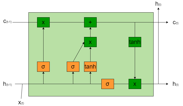
Figure 1: A standard LSTM cell.

The computational and memory demands of LSTM are higher than the traditional RNN’s, resulting in a large number of faster variants that emerged over the years. The most popular LSTM variant is Gated Recurrent Unit (GRU), with a slightly simplified architecture and an always-on output gate [45].

3.1.5 Encoder-Decoder Architectures and the Attention Mechanism

Any RNN/LSTM of one or more layers which unfolds across $K$ time steps accepts a sequence of $K$ input vectors in order to finally produce a corresponding sequence of $K$ output vectors. However, in a wide range of practical tasks the temporal lengths of the input/output sequences are not identical. If the length of one is $K$ while the other’s is 1, the problem is trivially solved by unfolding the network across $K$ time steps and considering only the final activation of the $K$-th time step as the network prediction. However, sequence-to-sequence mapping tasks between sequences of different lengths other than 1 are more complicated.

Typically, RNNs are adapted to solve such problems (e.g., machine translation) using a mixed Encoder-Decoder scheme. The input sequence is fed to a recurrent coding network which processes it over $K$ time instants (where $K$ is, e.g., the length of the input sequence), but only the final network output from the $K$-th time step is stored. Thus, it constitutes a coded vector (of fixed dimensionality equal to the number of the Encoder’s output neurons, independent of $K$) representing the entire input sequence. This vector is then fed to a recurrent decoding network unfolding across $L$ time steps ($L$ can be arbitrary and not necessarily equal to $K$ or 1). At the first time step of the Decoder’s inference stage it is given as input the coded vector. During the following time steps, its processing is based only on the stored internal state. The $L$ Decoder outputs constitute the final output sequence. The overall network is trained uniformly by BPTT.

As an improvement over this basic idea, the neural attention mechanism was introduced in [46] to allow the Decoder of a mixed Encoder-Decoder RNN architecture to consider all the outputs of the Encoder, and not just that of the last encoding time step, with a different weighting factor. These weighting coefficients, known as attention weights, are given by an attention distribution that the Decoder produces at each time step of its inference stage, in order to read selectively and at will the Encoder’s outputs according to its own current internal state. This is achieved by the attention mechanism: a differentiable and continuous way to access a sequence of stored discrete key vectors. Thus, the mechanism allows a neural network to learn suitable access patterns on its own from proper training on a dataset, through usual back-propagation and gradient descent optimization.

Attention operates by generating a continuous probability distribution defined over the entries of the key sequence. This distribution is produced in the following way. First, the network generates a query vector that essentially needs to be searched for in the key sequence. Then, the dot product of that query with each key vector is separately computed, with the ordered results essentially forming a new sequence of cosine similarities between the query and each key vector. This similarity sequence is converted to a probability distribution by passing it through a softmax function. Then, a weighted sum of all key vectors is generated, using the attention weights as coefficients. Optionally, this weighted sum can be computed on a different set of value vectors, instead of the key vectors through which the attention weights were estimated. Queries, vectors and keys can be derived by the DNN during inference through projecting given vectors (linearly or non-linearly) via learnt separate transformations. These operations are differentiable and their parameters are learnt while training the overall network with a typical, task-specific cost function. The process of constructing the weighted vector sum using the attention weights is referred to as the query attending to the keys and/or values.

In the case of Encoder-Decoder RNN architectures, the key/value sequence is the temporal sequence of Encoder internal states/outputs across $K$ time steps, respectively, while the $L$ separate queries are the Decoder’s internal states at each time step of its inference stage. Alternatively, the key and the value sequence may coincide. This setup allows the Decoder to read at each time step an aggregate context vector before it generates its current output: such a context is a parameterized summary of all $K$ Encoder outputs, adjusted according to the Decoder’s own current state.

3.1.6 Transformers

The Transformer architecture [47] was an attempt to replace RNNs for sequence-to-sequence mapping tasks, while simultaneously maintaining the mixed Encoder-Decoder scheme. Both the Encoder and the Decoder consist of $N$ consecutive macrolayers each. The Decoder operates at discrete time steps, with its final layer outputting at the end of each step the next element of the requested output sequence. Its first layer’s input at the beginning of each step is the output of its final layer from the previous step, i.e., the Decoder is autoregressive. However, the Encoder operates at a single pass, processing the entire input sequence at once. The first Encoder layer receives as its input a list of at most $K$ vectors, i.e., an ordered list of all elements/tokens in the input sequence. Each vector in this sequence is the sum of a suitable representation of the corresponding token (e.g., a sparse one-hot encoding of a word from the supported vocabulary) and a “positional encoding”, i.e., a dense vector representation of the index of the respective input token within the overall sequence. Each of the subsequent Encoder layers receives as its input a list of $K$ corresponding, transformed vectors, i.e., the outputs of the previous Encoder layer.

Each layer of the Encoder or the Decoder is composed of two consecutively placed sublayers: a self-attention sublayer and a succeeding small MLP. The self-attention mechanism enables the layer to process its input sequence in parallel, while the following fully connected layers transform the output of the self-attention process. However, a self-attention sublayer is itself composed of $M$ parallel, independent self-attention heads. Each head receives a linearly transformed version of each input vector as a query and two linearly transformed versions of the overall input sequence as a key and as a value sequence. Within a head, a common key/value sequence representation is utilized for all queries. The transformations are performed by multiplying each input vector with suitable weight matrices, separately learnt per self-attention head as model parameters. Thus, although all heads of one layer separately receive the same input sequence as a list of queries, of keys and of values, this sequence is differently transformed per head befored being fed to them. The output of each self-attention head is one new vector representation per input token, which inherently incorporates appropriate context information from the entire sequence. The outputs of all heads are concatenated and subsequently linearly transformed, using an additional learnt weights matrix, before being fed to the succeeding MLP.

The Decoder has a structure similar to the Encoder, but includes an additional, regular attention mechanism within each of its layers, for also attending to the Encoder’s final outputs. However, the use of both an Encoder and a Decoder is not strictly necessary in tasks that do not involve sequence-to-sequence mapping with input/output sequences of different lengths. The original Transformer’s Encoder-Decoder architecture is depicted in Figure 2.

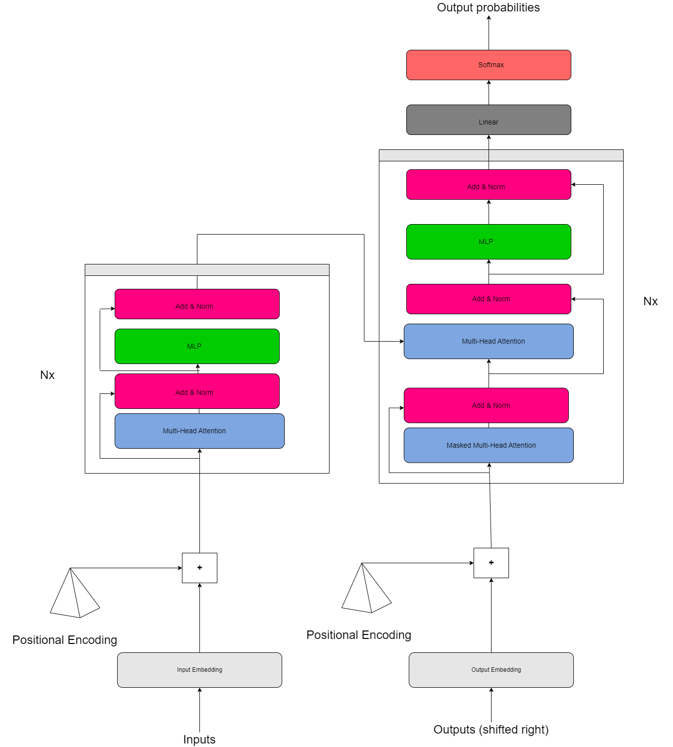
Figure 2: The original Transformer Encoder-Decoder architecture.

Overall, the simultaneous processing from multiple, parallel self-attention heads and the resulting lack of recurrence in the Encoder render the Transformer able to achieve faster training and inference times, compared to previous RNNs/LSTMs that process the input sequentially. Additionally, the learnable self-attention mechanism allows the Transformer to easily, selectively and adaptively capture contextual information and long-term dependencies from the entire input sequence, when analyzing each individual token during inference. Thus, Transformer layers effectively have a global receptive field from the get-go. Finally, the use of multiple self-attention heads per layer allows each layer to simultaneously compute multiple different representations from its input sequence, thus capturing different features at once.

Eq. (11) below succinctly captures the inference-stage processing of a self-attention head:

$$Attention(\textbf{Q},\textbf{K},\textbf{V})=softmax(\frac{\textbf{QK}^{T}}{\sqrt{d_{k}}})\textbf{V},$$ (11)

where $\textbf{Q}\in\mathbb{R}^{N_{q}\times d_{k}}$ are the $N_{q}$ queries, $\textbf{K}\in\mathbb{R}^{N_{k}\times d_{k}}$ are the $N_{k}$ keys and $\textbf{V}\in\mathbb{R}^{N_{k}\times d_{v}}$ are the $N_{k}$ values. Each query vector and each key vector has a dimension of $d_{k}$, while each value vector has a dimension of $d_{v}$.

Multihead self-attention can be formulated as:

$$Multihead(\textbf{Q},\textbf{K},\textbf{V})=[\textbf{h}_{1};...;\textbf{h}_{M}]\textbf{W}^{O},$$ (12)

where

$$\textbf{h}_{i}=Attention(\textbf{Q}\textbf{W}^{Q}_{i},\textbf{K}\textbf{W}^{K}_{i},\textbf{V}\textbf{W}^{V}_{i}).$$ (13)

In this formulation, $\textbf{W}^{Q}_{i}\in\mathbb{R}^{d_{a}\times d_{k}}$, $\textbf{W}^{K}_{i}\in\mathbb{R}^{d_{a}\times d_{k}}$, $\textbf{W}^{V}_{i}\in\mathbb{R}^{d_{a}\times d_{v}}$, $\textbf{W}^{O}_{i}\in\mathbb{R}^{Md_{v}\times d_{a}}$ are learnt parameter matrices, $M$ is the number of heads, $d_{k}=d_{v}=\frac{d_{a}}{M}$, and the operator $[;]$ implies concatenation.

Note that the softmax function in Eq. (11) is separately applied to each row of its argument, resulting in a matrix output. Each row of each $\textbf{h}_{i}$ matrix is a convex combination of the rows of $\textbf{V}\textbf{W}^{V}_{i}$, with the respective row of the output of the softmax providing the corresponding weighting coefficients. Scaling by $\sqrt{d_{k}}$ in Eq. (11) serves to ensure training stability.

3.2 Neural Building Blocks for Long Document NLP

3.2.1 Word Embeddings

Modern NLP algorithms typically require a very important preprocessing phase: during this phase, each input token is transformed into a semantically meaningful, fixed-size, dense vector, which is typically called word embedding. The resulting sequence of word embeddings is the actual input to the main DNN that executes the desired NLP task [48]. Such word embeddings are utilized both at the training and at the inference stage. One trivial way to achieve this is to simply append an initial embedding layer at the employed DNN architecture, which is subsequently trained end-to-end. Thus, the embedding layer receives the raw tokens as its input, e.g., as sparse, one-hot encoded vectors, and transforms them to a semantically meaningful, dense vector representation. However, the most widespread approach is to exploit pretrained, separate, dedicated embedding neural networks and utilize their outputs as dense word embedding vectors.

One of the most historically significant word embedding neural networks was Google’s Word2Vec [48]. It is a shallow MLP with one hidden layer, able to compute a useful representation of a word token in the form of a real, dense, fixed-size vector with a dimensionality equal to $H$, i.e., the number of hidden neurons in the model. Word2Vec[48] representations/embeddings have rich semantic content: words with similar or related meaning are mapped to vectors that are approximately parallel in the representation/embedding space (i.e., they have high cosine similarity), while applying typical vector operations to such representations is semantically meaningful (e.g., corresponds to semantic analogies between the represented words) [49].

The Word2Vec MLP receives as its input a non-semantic (e.g., one-hot) vector encoding of a word with a dimensionality of $L$ (equal to the supported vocabulary size). It has been pretrained according to the following self-supervised objective. First, for each occurrence of each significant word (e.g., nouns, verbs, adjectives, proper nouns) in the available training dataset/text corpus, the $D$ words immediately before and the $D$ words immediately after the one in question are selected. Each such mapping from a word to its $2D$ neighboring ones in the context of each occurrence is exploited as a training pattern/label pair, using typical error back-propagation and gradient descent. Thus, the co-occurrence of words within a given context is implicitly utilized to learn the relationships between these words.

The input/hidden/output layer has $L$/$H$/$2DL$ neurons, respectively. After the model has been trained, the output layer is discarded and the remaining network can be exploited to produce a semantically rich representation of each input word: this is a dense, $H$-dimensional real vector. Obviously, a very large data set is required to properly train such a model, and in Word2Vec’s case that was GoogleNews (100 billion words).

Other word embedding algorithms followed-up and improved upon the Word2Vec concept, such as GloVE [50]. However, the next significant milestone was the development of context-sensitive word embedding networks, which were able to generate different vector representations for a single word depending on its context, i.e., its position in a sentence. ELMo [51] was able to achieve this using an LSTM architecture, but it was Bidirectional Encoder Representations from Transformers (BERT) [52] which originally exploited the power of Transformers in order to significantly advance the relevant state-of-the-art. Such DNNs that learn to generate contextualized word embeddings, by being trained to predict the next word of an input sentence, are essentially language models.

3.2.2 BERT

BERT is a bidirectional, deep Transformer Encoder, without an attached Decoder. It receives an input sequence consisting of numerical representations of a text’s tokens/words (e.g., non-semantic indices to a supported vocabulary), to generate a corresponding sequence of refined, semantically encoded output vectors as this text’s representation. Initially, the special token [CLS] is externally appended to the beginning of the overall input sequence, so that its output semantic representation will aggregate global contextual information about the entire textual sequence. Also, the special token [SEP] is inserted after each input sentence to separate consecutive sentences. The ordered token representations are then transformed by a preliminary, trainable embedding layer. Subsequently, a learnt dense “segment embedding” vector and a learnt position embedding vector are added to the vector representation of each input token. Finally, the first actual Transformer layer receives these ordered vector sums as its input sequence. The segment embedding of a token belonging to the $i$-th sentence simply indicates whether $i$ is odd or even.

The output word embeddings have specialized semantic content in comparison to corresponding Word2Vec representations, i.e., adapted to the context of the specific input sentence. This is because the network processes a complete input text at each iteration of its training stage, taking into account all its words and their order at a single pass, through the self-attention mechanism. Thus, during inference, it processes each input word in the context of its bilaterally ordered phrasal contexts. Therefore, the same word in the context of different sentences, or even placed at a different position in an otherwise identical sentence, can be mapped to different embedding vectors by the pretrained network.

More difficult objectives are employed for pretraining BERT, compared to simply predicting the previous and next words of the current sentence, as in Word2Vec. These objectives are tailored to the Transformer’s special features. The most common goal is to predict a few randomly chosen masked words of a complete input sentence based on its remaining words. This is a “Masked Language Model” (MLM) pretraining objective, inspired by the Cloze task [53], where a subset of the input’s tokens are randomly masked, i.e., each one is replaced by a special [MASK] token, and the goal is to predict the original words based on the context. The MLM objective encourages the model to fuse the left and the right context and, thus, is particularly suited to deep bidirectional Transformers [52]. A complementary pretraining objective is to classify two jointly fed input sentences as either consecutive or non-consecutive ones (Next Sentence Prediction, NSP). This teaches BERT to understand longer-term dependencies across sentences. In both cases, after training the final prediction head or classification layers are discarded and only the trained Encoder is retained, to generate the word embeddings of input sentences.

A shallow, pretrained Word2Vec model encodes a fixed 1-1 mapping of words to representations/embedding vectors and, thus, can be used in a variety of NLP tasks only for feature extraction at a preprocessing stage. In contrast, a pretrained deep BERT model can optionally be adapted itself to the desired downstream NLP task, by appending appropriate additional final neural layers (usually fully connected or recurrent) and performing minimal fine-tuning on the overall network. During inference, BERT must be given as input a complete sentence, so as to generate the most contextually appropriate embeddings of its words. Due to the fixed maximum sequence size accepted by Transformers, BERT is restricted to receiving at most 512 tokens as its input text. Finally, a pretrained BERT comes with a dictionary of words it has been trained to embed. Thus, if during inference it is found out that the current word is unknown, it is broken into subwords which are considered by the network as different, consecutive elements of the input sequence (subword tokenization). In the case of compound words, such a subword is indeed potentially known, otherwise the token decomposition eventually reaches the level of the individual alphanumeric characters of the original word, which always belong to the known dictionary. The final representation of an input word can be derived as the vector average of the embeddings of its subwords. Thus, BERT can easily handle “unsupported” out-of-vocabulary words. Figure 3 depicts how the input to BERT is constructed.

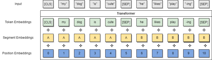
Figure 3: BERT input representation. The input embeddings are the sum of the token embeddings, the segmentation embeddings and the position embeddings.

3.2.3 ELECTRA

Various improvements over the original BERT have been proposed over the past few years. For instance, “Robustly Optimized BERT pre-training Approach” (RoBERTa) [54] aggregated several minor improvements in the training process and slightly modified the MLM pretraining objective, by dynamically changing the masking pattern applied to the training data.

One of the most significant recent improvements over BERT is “Efficiently Learning an Encoder that Classifies Token Replacements Accurately” (ELECTRA) [55], which was also motivated by the shortcomings of the MLM self-supervised pretraining objective. The latter “corrupts” the input sentence by replacing a small subset of its tokens with [MASK] and then training the model to reconstruct/predict the original ones. This requires a lot of training iterations/sample to be effective, since the task is essentially defined only over the masked tokens. Thus, ELECTRA proposed “Replaced Token Detection” (RTD) as an alternative self-supervised pretraining task. In RTD, the model learns to distinguish real input tokens from plausible but synthetically generated replacements: a randomly selected subset of the input tokens are replaced with synthetic alternatives (typically the output of a small language model), instead of being masked. The pretraining task is defined over all input tokens, since each of them has to be classified as original or synthetic. Learning from all input tokens leads to a learning process which is both much faster and more efficient; thus, ceteris paribus, ELECTRA achieves increased performance in downstream tasks due to better contextual word embeddings. Figure 4 graphically compares the MLM and the RTD tasks.

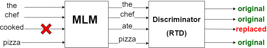
Figure 4: Graphical comparison between the MLM and the RTD tasks.

3.2.4 T5

T5 [56] is a renowned, general-use Transformer architecture for NLP. The modus operandi of T5 is to transform each desired NLP task, either discrimnative or generative, into a sequence-to-sequence mapping problem (text-to-text). Thus, it follows the standard Encoder-Decoder architectural paradigm, a design choice that allows it to easily handle input and output sequences of different sizes. This is unlike BERT, which is a bidirectional Encoder-only Transformer. Similarly to other language models, T5 is first pretrained on a large-scale corpus with a self-supervised objective, before being finetuned on the desired, typically supervised downstream task. Pretraining enables the model to learn general language patterns and representations, while downstream finetuning specializes it to task-specific nuances. Both training modes fall under the text-to-text format, therefore a common maximum likelihood loss function is employed regardless of the task.

The text-to-text nature of the architecture allows T5 to be pretrained with a masked language modelling objective that uses targets composed of multiple consecutive words per each [MASK] token. Unlike BERT, this is done through random corruptions of text segments with varying masking ratios and segment sizes. A simplified example of the T5 self-supervised objective is depicted in Figure 5. The use of a complete Transformer Encoder-Decoder architecture, coupled with this fitting self-supervised pretraining task and a very large-scale pretraining dataset, jointly permit T5 to achieve remarkable performance across a variety of different language tasks (e.g., document summarization, sentiment analysis, etc.), after proper finetuning.

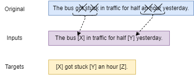
Figure 5: The T5 pretraining objective.

3.2.5 BART

Similarly to T5, BART [57] is also a Transformer language model that follows a full Encoder-Decoder architecture and is pretrained with a self-supervised sequence-to-sequence mapping objective. As in BERT, the Encoder is bidirectional and pretraining consists in mapping arbitrarily corrupted textual sentences to their original form. However, BART generalizes the BERT objective since a single [MASK] token can cover several consecutive target tokens (as in T5), while alternative corruptions are also possible. After pretraining, downstream finetuning can take place without any corruptions to the input. With this setup, BART achieves very good results in a variety of downstream language analysis tasks.

Notably, both T5 and BART utilize a full Transformer Encoder-Decoder architecture with an autoregressive Decoder and an inherent suitability to text-to-text mapping. An important consequence of this choice is that they can easily be finetuned for generative NLP tasks (text generation, e.g., for document summarization) without any architectural additions after pretraining, while this is not possible with the bidirectional Encoder-only BERT. In this sense, BERT and its derivatives can be considered deprecated as of 2023 [58].

3.2.6 GPT and Large Language Models

Recently, NLP algorithms employing pretrained GPT (Generative Pretrained Transformer) [59] neural models have been gaining a lot of traction. Similarly to other state-of-the-art language models, GPT is a large-scale autoregressive Decoder-only Transformer pretrained in a self-supervised manner and on a gigantic corpus for predicting the next token in a sequence. Due to this traditional causal language modelling objective, pretrained GPT models can be directly employed for text generation without any finetuning: they are given a text prompt as input and they generate a corresponding textual response as an output. Although pretrained GPT models can be finetuned in a typical supervised manner for a specific downstream task, their most impressive capability is that of zero/few-shot downstream language task execution during inference, through careful prompting and without any finetuning. In this case, the desired task is essentially described in natural language on-the-fly via the prompt. However, this setting falls outside the scope of this article.

When it comes to long document analysis, the latest openly available pretrained GPT model is GPT 2.0 [60], which remains regularly outperformed by BERT-derived language models, such as RoBERTa [61], in the finetuning setting. However, the publicity GPT models have attracted due to their text generation capabilities makes them a serious competitor for BERT and its variants. GPT 3.0 achieves similar results to most BERT-based language models [61], but is not openly available to the public. Similarly closed-source competitors to the GPT family do exist, such as [62], while open-source alternatives are BLOOM [63] and OPT [64]. The scale factor, i.e., highly complex Decoder-only Transformer DNN architectures and a gigantic pretraining corpus/dataset, has proven instrumental for obtaining good performance in all the above cases of Large Language Models (LLMs). However, the observation that scaling up the DNN architecture is only beneficial when accompanied by a corresponding increase in the dataset size has recently led to more reasonably sized models of this nature, i.e., less complex ones, such as Chinchilla [65] and LLaMA [66].

Table 2 showcases the escalation of language model complexity in recent years.

Name	Year	#Parameters	Input Size (#tokens)
BERT	2019	110M	512
BART	2019	140M	1024
T5	2019	Up to 11B	512
GPT	2018	120M	-
GPT-2	2018	1.5B	1024
GPT-3	2020	175B	4096
BLOOM	2022	176B	-
OPT	2022	125M to 175B	-
PALM	2022	540B	3072
Chincilla	2022	70M to 16B	-
LLaMa	2023	7B to 65B	2048

Table 2: Comparing modern language models by model complexity and input tokens limit (where available).

4 Document Classification

Document classification is the automatic assignment of one or more class labels to a piece of text, based purely on its contents and assuming a known finite set of discrete labels. In long document NLP, the text in question is typically an entire document. As an example, a book of fiction could automatically be assigned a genre label by a text classifier deployed in a library, supporting labels such as “Romance” or “Science Fiction”.

Overall, recent methods for neural long text/document classification mostly rely on pretrained Transformer language models (e.g., BERT) with a classification head appended at the end. The language model may be finetuned for the desired downstream classification task, while training the head. This approach is suitable for most relevant tasks [25] [67] [68] [69] [70] [71]. However Transformers may be suboptimal for specialized tasks or domains [72], allowing CNN and RNN architectures to occasionally outperform them on long documents. Relevant issues and solutions are discussed below.

4.1 Challenges

Long text classification algorithms inevitably face challenges that are common to all NLP tasks, as well as issues specific to the case of long texts. Below, follows a non-exhaustive list of the most significant relevant challenges:

• Input size. The size of the input document is the most significant challenge in long document NLP. For example, the computational overhead of CNNs tends to grow proportionally to their inputs; thus, they are unable to process documents with thousands of sentences, without specialized hardware. On the other hand, RNNs/LSTMs struggle to conserve information and identify long-term dependencies over huge spans of text [73]. Transformer DNNs, such as BERT and most of its variants, are typically constrained by a rather low maximum token sequence length; usually 512 or 1024 tokens. This limits their training to relatively short texts, forcing brutal token selection during inference. As a result, their performance on long texts is severely limited [74]. Additionally, traditional Transformer architecture [47] rely on the typical global self-attention mechanism, comparing each token to all other input tokens at each self-attention head, leading to a quadratic ($O(n^{2})$) increase in computational and memory requirements with respect to input size.

• The curse of dimensionality. As the supported vocabulary increases in size, the possible inference-stage combinations of its words grow exponentially large, unlike the fixed training dataset size.

• Polysemy. A word may express multiple different meanings in different contexts. For example the word “bank” may mean a financial institution or a building. DNN models must learn to appropriately differentiate the exact meaning of a word depending both on the local context (sentence, paragraph) and the global context (document).

• Homonymy. Homonyms are words that either share spelling (homographs), pronunciation (homophones) or both, but are not semantically related. For instance, the term “bank” may refer to a financial institution or to the shore of a river. The difference between homonymy and polysemy is that homonyms are not at all related to each other in meaning.

• Figurative language. Sarcasm, irony and metaphors pose serious challenges to NLP, since the real meaning of a phrase is different from the immediately obvious one [75]. Figurative language is common to both short and long texts, but in the latter case it can take the form of sustained allegories (e.g., in literary books).

• Unstructured text. Long texts may be very unstructured for the most part, while communicating information in rather indirect and abstract ways. For example consider a novel, partitioned in a few dozens of chapters, and contrast it with short texts, such as product reviews or tweets. In the first scenario, crucial information and layers of meaning may be distributed across a large number of very long chapters [1]. Furthermore, long documents tend to follow constantly evolving textual and contextual conventions, leading to a higher chance of shifts between learnt and actual probability distributions. This is especially problematic for literary works, which are fluid and susceptible to changing cultural biases [76].

• Multiple labels. The longer an input document is, the more probable is that it belongs to multiple classes concurrently. Classifiers should specifically take it into account for meaningful analysis, since each document may have a varying numbers of ground-truth labels.

• Foreign language datasets. There is limited availability of training content for languages other than the most popular ones (e.g., English, French, Spanish, etc.). Given that both the word embedding networks and the main, task-specific NLP DNNs are typically trained on one language at a time, the lack of extensive datasets in rarer languages leads to less optimal embeddings and, as a result, reduced performance in downstream tasks. The situation is aggravated by limited training sets for the downstream tasks themselves. Thus, less data-intensive machine learning algorithms may be preferred over DNNs for rare-language texts, such as decision tree classifiers [76], or the existing datasets can be artificially augmented [77].

4.2 Solutions

Traditional machine learning algorithms, such as Naive Bayes [78], SVMs (Support Vector Machines) [79] and ID3 decision trees [80] have been repeatedly applied for document classification [76] [81], being competitive even in large literary texts [82]. However, the field has generally moved decidedly towards DNNs and this Subsection presents the relevant state-of-the-art. The innovations of the various existing approaches mostly fall under the following categories, which are more or less tied to the challenges mentioned in Subsection 4.1:

4.2.1 Multi-label Classification

Multiple labels are essential for many real-world applications [83] [84], thus many methods attempt to identify a document as belonging to multiple classes concurrently. This may be trivial to achieve in itself, using well-known DNN models that have been properly adapted. The varying number of labels per document and class imbalance issues, which may lead to learning extremely biased patterns from the training data, can be handled by applying weighted loss functions. However, multi-label classification poses unique challenges with regard to how accuracy is measured.

One representative state-of-the-art approach attempting to tackle this scenario is [82], where multiple different classifiers (including a pretrained BERT) are comparatively evaluated in multi-label multi-class document classification, using the book genre recognition task as a benchmark. The steps taken in [82] to build a successful genre recognizer are telling of more general difficulties with long document classification. Regarding the issue of multiple labels, a modified accuracy metric is exploited to measure classification accuracy: the true positive and true negative classifier predictions are first computed separately per class label, with the proposed metric being the weighted average of correctness over all the label classes. Per-class weights are proportional to the class label frequency and normalized to sum to 1. Similarly, the loss function employed during training (Binary Cross Entropy) is modified to include weights for each label, so that each class is scaled inversely to the prominence of the class in the training set.

4.2.2 Feature Pruning

This is the traditional way to handle long textual inputs. It involves systematically discarding as much text as possible at the preprocessing stage, while minimizing information loss. In order to cope with the potentially huge input size in long document analysis, almost all relevant NLP methods are prefaced by a preprocessing stage, where less useful input elements are removed. Appropriately reducing the input size improves both computational efficiency and accuracy. To this end, the book genre recognizer of [82] uses an aggressive sampling method which first discards:

• “stopwords”, i.e., known, extremely frequent words such as “a”, “and”, “he”, etc.,

• words that appear less than 20 times,

• words that appear in more than 75% of all books,

• words that appear in more than 75% of all classes,

• paragraphs where the frequency of the remaining words is less than a certain threshold,

• the contents of each remaining paragraph after the 512th token, because of technical limitations imposed by BERT.

Thus, each remaining paragraph is represented by a subset of its words that fall within a restricted, book-level set of “keywords”. Finally, the sampled paragraphs are only those with the highest concentration of keywords. The goal of this ruthless sampling is to keep the input’s length manageable for documents containing many thousands of pages. Methods similar or identical to this one are present in most NLP models specialized for long texts; thus, they are utilized extensively in most research cited in this paper.

On the other hand, the book genre recognizer of [1] employs only minimal preprocessing, just enough to allow the DNN to run relatively efficiently. It relies on an index, consisting of the 5000 most common words from the supported vocabulary. No other preprocessing/sampling takes place, under the intuition that exposing the DNN to even statistically unimportant words facilitates an understanding of patterns and grammatical modifiers, such as tense and plurality. Words are represented by typical neural embeddings. Different strategies were evaluated for feeding the document to the classification DNN:

• Feed only the first 5000 words of the document.

• Feed only the last 5000 words of the document.

• Feed only 5000 random words of the document.

• Feed the entire document, split into chapters.

• Utilize a traditional bag-of-words approach.

These strategies were then employed on a series of different architectures. Ultimately, the random word selection proved to consistently outperform other selection strategies for a multitude of classifiers, with the best performer being a CNN-Kim [85] architecture.

4.2.3 Sparse Attention Transformers

Given the quadratic computational complexity of Transformer DNNs and their prominence in recent years, attempts have been made to reduce their cost. Such approaches try to achieve linear complexity with respect to the input size, by keeping track of a small, fixed-size window of neighbouring tokens around each input token, instead of considering all $n$ tokens of the input sequence within each self-attention head. However, the unavoidable trade-off is a reduced ability of the DNN to capture long-term dependencies, which is as important for long texts as the complexity with respect to the input size. Below, the terms token and element are used interchangeably, although strictly speaking only the first Transformer layer receives actual tokens as input (e.g., word embeddings).

4.2.3.1 Sparse Transformer

The Sparse Transformer was introduced in [86], so as to lower asymptotic complexity from $O(n^{2})$ to $O(n\sqrt{n})$. This is done by applying sparse factorizations to each self-attention matrix computed by the Transformer during inference, which contains the current attention weights of each input element against each of the other elements of the input sequence. Given that such a matrix is separately constructed at each self-attention head of each layer, it is important to effectively reduce the computational and memory cost of this operation. The sparse attention mechanism relies on replacing full attention with several small, optimized attention operations, which jointly approximate the original mechanism sufficiently. Essentially, each token attends to only a subset of the overall input sequence tokens. Additional optimizations, such as efficient sparse attention kernels and improved weight initialisation contribute to a less demanding architecture, which is thus able to handle longer sequential inputs. The Sparse Transformer is a general model suitable for various applications involving very long input sequences, ranging from image compression to document analysis.

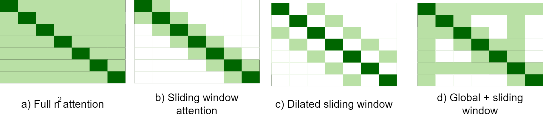
Figure 6: Comparing the full self-attention pattern and the configuration of attention patterns in a standard Longformer.

4.2.3.2 Longformer

Surpassing the Sparse Transformer’s computational gains, the Longformer [87] achieves a linear asymptotic cost and is specialized for long document NLP. Its self-attention mechanism can be directly incorporated within other Transformer models and operates by employing a dilated sliding attention window, which is a modification of the classical sliding window approach for local attention [88, 89]. In the typical case, each token’s window is comprised of $w$ tokens surrounding it: $\frac{w}{2}$ tokens to its left and right, respectively. The underlying intuition is that the semantic context of a token can be mostly derived from its neighbouring tokens, while the computational complexity of this operation is $O(n\times w)$. In a sense, the end effect resembles the local receptive fields of neurons in convolutional layers. Similarly to CNNs, stacking $l$ Longformer layers gradually increases this receptive field, so that representations of tokens faraway from the query can be attended within the later layers.

The dilated sliding window approach modifies the sliding window with a predetermined dilation factor $d$ added at each step, which determines the spacing between adjacent window positions and allows data analysis at multiple scales simultaneously. Thanks to the introduced “gaps” in the attention pattern, a larger range of tokens within the self-attention matrix can be covered without increasing calculations and computation time. Thus the effective receptive field of the window is of length $l\times d\times w$, while memory and processing costs remain steady.

Since windowed and dilated attentions may not be enough to extract a suitable sequence representation, certain additional, pre-selected locations of the full self-attention matrix are also allowed to be considered as global context. These global tokens attend to/are attended by the entire sequence as normal, but their number is kept constant and relatively small so as to limit complexity to $O(n)$. The [CLS] token is a good candidate for being selected as a global one, since its generated representations should convey information about the entire sequence. Overall, as a result of Longformer’s innovations, it has been successfully evaluated with inputs of length up to 4096 tokens (compared to BERT’s maximum of 512 tokens). A comparison between full, sliding, dilated sliding and global-dilated sliding window self-attention patterns is depicted in Figure 6.

4.2.3.3 BigBird

BigBird [90] can be seen as a variation of the Longformer, attempting to support much longer input sequences by reducing the complexity of self-attention from quadratic to linear. It also employs a sliding window, since in typical NLP tasks the semantic context of a token can be mostly derived by its neighbouring tokens. Instead of the Longformer’s dilated sliding windows, it employs random token selection to reach faraway tokens and provide context. This complements the global attention and the regular sliding window attention schemes, adopted and adapted from the Longformer. It has been demonstrated mathematically that this modified sparse attention mechanism satisfies many theoretical properties of the original full attention mechanism, such as universal approximation and Turing-completeness, but seems to require more layers to retain accuracy comparable to full attention architectures.

4.2.4 Hierarchical Transformers

Hierarchical models attempt to handle the large input size of long texts by appropriately building upon original Transformers, instead of modifying them. This is usually achieved in one of two ways:

• By transforming the Transformer’s input via a suitable DNN (e.g., a CNN or RNN/LSTM). The latter one generates a single document representation (document embedding) able to fit into a standard Transformer (e.g., BERT), thus bypassing the input size limitations.

• By segmenting the input document. The input segments are independently truncated to the Transformer’s input size and the network (e.g., BERT) generates embeddings for each of these segments. A separate DNN then combines the segment embeddings and predicts the document label.

4.2.4.1 Hierarchical Attention Network (HAN)

The first attempt towards a Hierarchical Transformer [91] [92] was built on top of standard BERT. During inference, the input document is split into paragraphs that are truncated to fit into BERT. The latter one generates independent paragraph embeddings, which are combined by the succeeding HAN into a single output. The end result is an increased ability to handle long texts, by exploiting the natural partitioning of documents into paragraphs.

A similar approach was later used in [93], where the base models were BERT, RoBERTa, DeBERT [94], Legal-BERT [95] and CaseLaw-Bert [96]. In long text analysis tasks, the hierarchical versions proved competitive with Sparse Attention Transformers, such as Longformer and BigBird.

The method in [97], relying on BERT or on Universal Sentence Encoders (USEs) [98] (models learning sentence representations for transfer learning), follows up on this methodology, but replaces the final HAN with a CNN or an LSTM architecture. The BERT+LSTM combination proved to be the best among the evaluated hierarchical approaches, which however were generally outperformed by Sparse Attention Transformers.

4.2.4.2 Hi-Transformer

The main alternative to [93] and its variants is to essentially reverse the process: that is, to employ a hierarchical DNN for obtaining a fixed-size document-level representation/embedding from the entire input, which is then fed to a regular classification DNN. Hi-Transformer [99] achieves this via a Transformer acting as a “Sentence Encoder” (SE), i.e., aggregating and projecting the regular, individual word embeddings of the input document into sentence-level embeddings. Once every sentence has passed through SE, these embeddings are subsequently ordered by positional embedding and fed as input to a subsequent Transformer called “Document Encoder” (DE). The latter’s output is a context-aware document embedding, which is fed as input to the next SE along with the original sentences. Thus, the generated, revised sentence embeddings are aware of the global, document-level context. This process is repeated by stacking multiple such layers, until the final output is passed to a pooling layer that extracts the final document embedding. According to [99], two such layers seem to be sufficient for outperforming Sparse Attention Transformers in long text analysis. This can be attributed to the readily accessible global/document-level context. Since the final classifier has to analyze a fixed-size document representation and the SE’s complexity is linear to the number of sentences, computational demands are not higher than in the sparse attention case. More impressively, Hi-Transformer’s accuracy has been observed to actually increase with longer documents, since more relevant context can be extracted.

4.2.4.3 Hierarchical Sparse Transformer

Hierarchical Transformers have been combined with the sparse attention mechanism, in order to ameliorate the latter’s inability to capture all the necessary global/document-level context, in the case of long texts. This inability arises from the low level of global context diffusion in the generated token representations, since the global tokens are limited in number. The ERNIE-SPARSE architecture [100] merges the two schools of thought by using hierarchical attention, which is then fed to a Sparse Transformer in order to increase the information extracted from the global context.

ERNIE-SPARSE utilizes a modified attention mechanism, where each query is allowed to attend to a limited number of additional representative tokens within each fixed-size window of the self-attention matrix, along with regular global and local tokens from the input sequence. These inserted representative tokens carry global context from the entire document and are derived in two steps: first, the regular Sparse Transformer is applied to the unaltered input sequence and, then, regular full self-attention is applied to a small collection of selected outputs. ERNIE-SPARSE has been shown to outperform the competition on well-known document classification datasets. It can be considered both a hierarchical and a sparse attention approach, since it modifies the Transformer’s internal architecture. Figure 7 depicts the modified attention mechanism of ERNIE-SPARSE, in comparison to that of the Sparse Transformer.

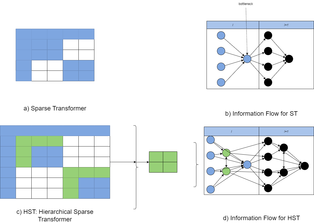
Figure 7: Comparison of Sparse Transformer (ST) and Hierarchical Sparse Transformer (HST). (a) Sparse Transformer comprises global attention and local attention. (b) ST faces a limitation where all sequence details are compressed into a fixed vector size. (c) HST addresses this limitation by incorporating representative tokens into local attention, enabling hierarchical attention. (d) The information flow in HST demonstrates how the interaction among representative nodes can enhance global information interaction pathways.

4.2.5 Recurrent Transformers

The fixed input size of baseline Transformers leads, during both training and inference, to context fragmentation in long document analysis: essentially, the DNN analyzes the input as independent, consecutive segments. Thus, a complementary direction of the state-of-the-art is to allow the Transformer to learn and extract long-term dependencies beyond the preset fixed input sequence size, while maintaining linear computational complexity and retaining local and global context.

4.2.5.1 Transformer-XL

The Transformer-XL architecture [101] introduces recurrence into the Transformer, thus integrating the RNN concept of retained hidden states. These states are passed within the Transformer from one segment to the succeeding one, thus effectively transmitting the previously established context and allowing the identification of long-term dependencies across segments. Unlike RNN/LSTM recurrence, where each layer’s stored state is exploited at the next time step by the same layer, the corresponding Transformer-XL mechanism shifts the transmitted state one layer downwards. For example, layer $l=n$ has access to 2 hidden states from layer $l=n-1$, 4 hidden states from layer $l=n-2$ and $2^{n}$ from layer $l=1$, which are the original input word embeddings.

This mechanism guarantees $O(n\times l)$ cost, where $l$ are the number of layers, and significantly faster inference compared to baseline Transformer, since representations computed for previous segments are re-used instead of being computed from scratch for each new segment. It also allows different input sequence sizes between the training and the inference stage. Ultimately, Transformer-XL achieves competitive results on extremely long document analysis, while being significantly more efficient than the baseline Transformer.

4.2.5.2 ERNIE-Doc

ERNIE-Doc [102] builds upon Transformer-XL but makes two passes over the input sequence, similarly to how humans first “skim” a document before paying attention to important sections. To achieve this, the cached hidden state is computed as follows:

$$\hat{\mathbf{H}}=[\hat{\mathbf{H}}^{1}_{1:T};...;\hat{H}^{N}_{1:T}]\text{ (skim phase)}$$ (14)

$$\tilde{\mathbf{h}}_{r+1}^{n-1}=[\tilde{\mathbf{H}};\mathbf{h}_{r+1}^{n-1}]\text{ (retrospective phase)},$$ (15)

where $T$ is the number of consecutive document segments, $L$ is the length of the document, $N$ is the number of layers. $\hat{\mathbf{H}}^{i}_{1:T}=[\hat{\mathbf{h}}^{i}_{1};...;{\mathbf{h}}^{i}_{T}]$ is the concatenation of the $T$ cached hidden states initially derived in the skimming phase for the $i$-th layer. Thus, $\tilde{\mathbf{H}}\in\mathbb{R}^{(LTN)\times d}$ is the concatenation of all $\hat{\mathbf{H}}^{i}_{1:T}$ (one per layer), Thus, context from the entire document can be exploited in the retrospective phase in order to form the extended hidden state $\tilde{\mathbf{h}}^{n}_{t}$.

This skimming architecture is incompatible with the recurrence mechanism from [101] and, due to its linear cost with regard to the number of layers, it may be prohibitive for long documents. To solve this, [102] “flattens” the hidden state dependency from one-layer-downwards recurrence to same-layer recurrence, similarly to RNNs. Additionally, a novel, document-level task for self-supervised pretraining is introduced that is called “Segment-Reordering Objective” (SRO). It entails randomly splitting a long document into $m$ segments, shuffling them, then letting the Transformer reorganize them in order to learn their interrelations. After pretraining on both the MLM task and on SRO, ERNIE-Doc proved highly competitive in several long document analysis datasets for a range of tasks such as classification, question answering and key-phrase extraction. Figure 8 depicts the modified recurrent mechanism of ERNIE-Doc, in comparison to that of basic Recurrent Transformers.

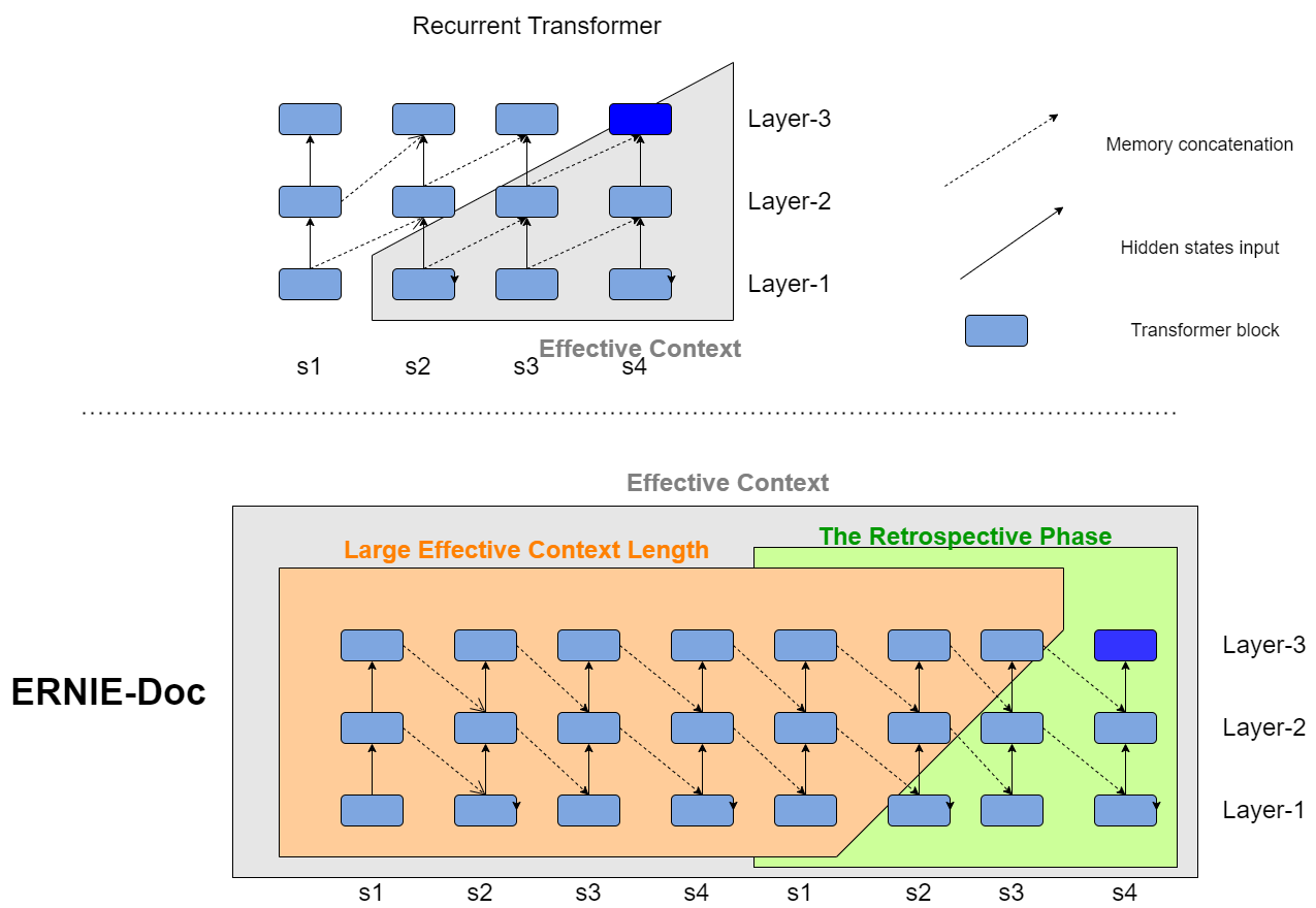
Figure 8: Comparison of 3-layer ERNIE-Doc and Recurrent Transformer, assuming a long document $D$ that is divided into four segments (S1, S2, S3, S4). Recurrent Transformer (upper): While training on S4, it can only incorporate contextual information from the preceding two consecutive segments, S2 and S3, due to the linear growth of the effective context length in relation to the number of layers. ERNIE-Doc (lower): With the assistance of an enhanced recurrence mechanism, the effective context length is significantly increased. Consequently, S4 can assimilate the information from S1, which was discarded by the Recurrent Transformer. Segments in the retrospective phase contain the contextual information of the entire document.

4.3 Sparse, Hierarchical or Recurrent Transformers?

Sparse attention, hierarchical and recurrent approaches dominate the current literature for long document analysis using Transformers. However, a number of challenges remain such as the following ones:

• Sparse Attention Transformers tend to suffer in accuracy, due to their reliance on a small number of global tokens that must encapsulate all document-level context.

• Hierarchical Transformers are particularly susceptible to context fragmentation, since the individual segment embeddings are derived either without sufficient local context [74], or with no access to the global document context [99].

Currently, there is no consensus on which approach performs better, nor any empirical rule on which tasks each architecture performs best in. Hybrid algorithms and recurrence seem to be the most promising avenues for advancing long text analysis.

5 Document Summarization

Automatic Text Summarization (ATS) is the task of generating a short summary from a source input document. In the context of long documents, such as medical and legal records, it is often called “document summarization”. The generated summary must be coherent, concise and avoid redundancy, while accurately maintaining the meaning of the most important information in the source material. There are two main approaches to ATS: extractive and abstractive summarization.

Extractive summarization generates its summary by selecting verbatim sentences found in the source text. This practically reduces summarization into finding a binary selection vector $\mathbf{s}=[s_{1},s_{2},...,s_{n}]^{T},s_{i}\in\{0,1\}\forall i\in[1,n]$, where $s_{i}=1$/$s_{i}=0$ if the $i$-th source input text sentence is/is not included in the summary, respectively. The simplicity and the tolerable computational cost of this approach have made it very common for on-line article summarization. However, its applicability is inherently limited by the fact that not all document types can be summarized well by just a few of their sentences taken verbatim and re-arranged. For example, there is no way to describe the content of most books by using a selection of their own sentences. Additionally, concerns have been raised that simple extractive approaches are reaching their peak and, therefore, current research should gravitate towards: a) ensembles of multiple extractive models, or b) abstractive summarization methods [103].

Abstractive summarization is the alternative approach of generating new text. It is the method humans use when trying to manually summarize text, by reading the source, extracting its meaning and then writing a condensed document which contains as much of the source’s meaning as possible. As expected, modern abstractive algorithms are DNNs [104]. Compared to extractive alternatives, they generate more meaningful and condensed summaries, while being more adaptable to the input document type. However, there is a much larger risk of the output summary misrepresenting facts and/or not being coherent at all. The most commonly used method for abstractive summarization involves employing a sequence-to-sequence mapping (Seq2Seq) model [105], via an Encoder-Decoder DNN architecture. RNNs and Transformers have both been employed in this context, where the Encoder captures suitable representations of the document’s tokens and feeds them to the Decoder that generates a summary.

5.1 Challenges

Document summarization comes with its own set of challenges. These are essentially specific to the case of long texts, since there is typically no reason to summarize a short text. Yet, a subset of them are shared with the challenges faced by long document classifiers.

• Input size: The length of the input document gives rise to significant issues which go beyond simple computational and hardware requirements. Extractive DNNs particularly struggle with long documents [106]; the greater the length of the input, the more topics it typically covers, thus the harder it is for a DNN to generate a summary covering effectively all of them.

• Evaluation metrics: The ROUGE evaluation metric [107], which is the most commonly used metric for summarization tasks, might not be sufficient for abstractive DNNs. It has been claimed to perform considerably worse than in the case of extractive summarization, since it lacks semantic understanding of the words it compares [108].

• Sentence extraction: Framing extractive summarization as a binary decision task assumes that the meaning of individual sentences is independent from that of others, leading to high redundancy. Even accounting for this fact, such DNNs are still vulnerable to greedily picking general sentences, instead of finding a combination of specific sentences which together summarize the document much more effectively [109].

• Repetition: One of the most common issues of abstractive DNNs dealing with long texts is sentence repetition; this is potentially caused by the over-reliance of a Decoder to its input, which gives rise to an endless loop of phrase repetition [110]. Internal issues concerning RNNs with attention mechanisms have been pointed out as the root cause of both this issue and of false information appearing in the output summary [111].

• Transformer issues: Most relevant state-of-the-art deep neural architectures feature the Encoder-Decoder pattern, implemented via Transformers. The challenges plaguing Transformer architectures such as BERT have already been largely analyzed in Section 4.1. Many of these remain as equally critical issues in long document summarization as well.

5.2 Solutions

This Section reviews the commonly employed ROUGE evaluation score, as well as extractive and abstractive text summarization methods. The evolution of relevant algorithms, as well as how each family attempted to handle the challenges it faces, are briefly discussed.

5.2.1 Evaluation Metrics

ROUGE is a very commonly used metric for evaluating ATS algorithms, featuring as many as 192 variations. The base ROUGE metric [107] measures the number of overlapping n-grams/sequences between the generated and ground-truth summary. This is sufficient for many extractive summarization tasks, but faces severe challenges when used for abstractive summarization. ROUGE is unable to distinguish between different grammatical versions of the same word [111] and synonyms [108], while being agnostic towards sentence ordering [112]. Most importantly, the underlying assumption made by ROUGE, that the quality of a summary is correlated to its coverage compared to the human-generated summary, may not be statistically significant [113].

The reasons why ROUGE is still popular despite such severe drawbacks are multiple, including the unavailability of proven competitors and the lack of easy-to-use software implementations or standardized benchmarks for ATS evaluation [114]. Besides, alternative metrics may suffer from similar weaknesses, since they typically do not account for factual consistency between the source document and its evaluated summary [115]. For a detailed discussion of text summarization metrics, the reader is referred to [114]. For the purposes of this article, a number of common and/or recent alternatives to ROUGE are briefly mentioned below:

• METEOR [116] (recommended by [111]), functions similarly to ROUGE, while being largely invariant to grammatical variants and synonyms.

• Sem-nCG [108] is a recent, semantically-aware metric focused on extractive summarization.

• BERTScore [117] uses the similarity of the contextual embeddings between the generated and the ground-truth summaries.

• $S^{3}$ [118] combines other evaluation metrics through a model, in order to produce an aggregated evaluation of the summary.

• BLANC [119] is an unsupervised evaluation metric which does not depend on human-generated ground-truth summaries, by comparing BERT’s performance on the Cloze task (on the source document) when it has and when it has not additional access to the generated summary.

Many more evaluation metrics have been proposed, but none has taken foothold yet. The question of a capable successor to ROUGE is still an open one.

5.2.2 Extractive summarization

This Subsection presents the gradual evolution of extractive summarization DNNs towards the current state-of-the-art.

5.2.2.1 Building Summaries Using Hierarchies

The first attempts to use DNNs for extractive summarization, while certainly obsolete today, developed core concepts that were later re-used and improved.

Thus, the method in [120] developed a neural Encoder-Decoder architecture, which is trained in a supervised manner by preprocessing human-written summaries to construct extractive ground-truth summaries (binary selection vectors). Architecturally, the Encoder is composed of a shallow CNN, called “Convolutional Sentence Encoder”, and a subsequent LSTM, called “Recurrent Document Encoder”. The first one analyzes a matrix of Word2Vec word embeddings, separately for each sentence of the source text, aggregating them to dense sentence embeddings. The second one sequentially receives these embeddings as input and generates a document-level embedding in the form of a fixed-size vector.

The Decoder is one of two models following different, mutually exclusive strategies: a “Sentence Extractor”, which approaches the extraction task as a sentence selection problem, and a “Word Extractor” which approaches it as a word generation task. The latter one is practically a limited-efficiency abstractive summarizer, with its supported vocabulary constrained to that of the source document, so it will not be detailed here. The Sentence Extractor is an LSTM-MLP combination, sequentially labeling individual source sentences for inclusion in the summary based on two criteria: i) whether they are relevant, and ii) whether they are mutually redundant with other sentences. The selection decision for the $t$-th sentence is computed as follows:

$$\mathbf{\hat{h}_{t}}=LSTM(p_{t-1}\mathbf{s_{t-1}},\mathbf{\hat{h}_{t-1}}),$$ (16)

$$p_{t}=\sigma(MLP(\mathbf{\hat{h}_{t}};\mathbf{h_{t}})),$$ (17)

where $\hat{\mathbf{h}}_{t}$/$\mathbf{h}_{t}$ is the Extractor’s/Encoder LSTM’s hidden state for the $t$-th sentence/time step, respectively. $p_{t-1}$ represents the assigned probability that the previous sentence $\mathbf{s}_{t-1}$ belongs to the summary and ; is the concatenation operation.

Following-up on [120], “SummaRuNNer” [121] was proposed as an extractive summarization RNN with the useful ability to be directly trainable on abstractive ground-truth summaries. It contains multiple layers of bidirectional GRUs and a hierarchical Encoder. Similarly to [120], the first subnetwork generates sentence embeddings from individual word representations, which are sequentially fed as input to the second GRU. The latter one analyzes them and outputs a document-level embedding from the sentence representations; this is done by average pooling the second subnetwork’s hidden states. The Decoder is simply a logistic binary classifier, assigning to each source sentence a “summary”/“non-summary” label. To be directly trainable on datasets with abstractive ground-truth summaries, a separate RNN Decoder can be optionally attached to the Encoder only during training and tasked to emit the most probable word at each time step. Figure 9 depicts the SummaRuNNer architecture.

Figure 9: The SummaRuNNer architecture. Bidirectional RNNs are represented by double-pointed arrows.

The method “LSTM-Ext” [106] improves on [120] and [121] by considering both global and local context information along with each sentence, in order to decide on its inclusion into the generated summary. Inspired by how humans read lengthy text, it was reasonably hypothesized that hierarchical information could benefit ATS. The “LSTM-minus” algorithm [122] is applied to generate local context-aware embeddings at the section level. Similarly to [120] and [121], an Encoder-Decoder architecture is employed. The Encoder is again composed of a Sentence Encoder (SE) and a Document Encoder (DE), but now also includes a “Topic Encoder” (TE) that provides access to local (section) context surrounding each sentence.

SE is a GRU that maps input word embeddings to a fixed-size sentence-level vector, while DE is a bidirectional GRU that encodes the sentence embeddings into a document-level vector representation. The final document embedding is computed as the concatenation of the final hidden states of the backward and the forward GRU. TE [122] separately embeds local context about each sentence’s section by employing the LSTM-minus method; the result is an additional vector per section. Subsequently, for each sentence, the embeddings of itself, of its section and of the entire document are concatenated, optionally with weights assigned by an attention mechanism, and fed to the Decoder. The latter one is simply a binary MLP classifier that predicts whether each sentence should be included in the summary or not.

The architecture’s efficiency seems to increase with increasing document length, making it a powerful architecture for long documents, while the most benefit comes from the use of local rather than global context. Thus, LSTM-Ext was among the first modern document summarization methods that explicitly handle the fact that longer texts tend to cover multiple topics. On the other hand, it is not designed to avoid unnecessary repetitions in the generated summary, resulting in outputs with potentially high redundancy.

5.2.2.2 Hierarchical Summaries using BERT

In recent years, Transformer and BERT variants gradually replaced RNN and Word2Vec/GloVe variants in extractive summarization. However, older ideas have been retained and improved, with their efficiency increased in an attempt to resolve long-standing challenges of document summarization.

The method in [123] uses BERT for both extractive and abstractive summarization (BERTSUM-EXT and BERTSUM-ABS, respectively). Instead of using sentence-level vector representations/embeddings, BERT inherently generates individual token representations. Thus, BERTSUM-EXT inserts special [CLS] tokens in-between sentences as separators, to notify the DNN of distinct sentences and capture sentence-level context within the respective generated token representations. This modified pretrained BERT is utilized as the Sentence Encoder component within an Encoder-Decoder architecture. The Document Encoder is a Transformer that receives the sentence-level embeddings of the [CLS] tokens that are derived by BERT and transforms them so as to contain richer document-level context. The final resulting sentence embeddings are fed to a shallow, fully connected binary classifier that predicts whether each sentence is to be included in the summary or not. All input documents are truncated to a fixed number of supported tokens. The overall architecture is finetuned in a supervised manner, using ground-truth binary selection vectors.

Despite the relatively strong performance of BERTSUM-EXT, it faces the typical challenges encountered by Transformers in long document analysis, such as varying and diverse topics. To counter this, the approach in [124] extends BERTSUM-EXT by taking advantage of the usually strong hierarchical structure of long texts (individual sentences compose titled sections, which jointly form the document). Thus, it computes hierarchical positional embeddings that capture the relative position of a token within each section and the position of that section in the document. These representations, along with additional representations of the section titles, are incorporated into the sentence-level embeddings by the Document Encoder, which feeds the final shallow, fully connected binary classifier. Of course, the overall “HiStruct+” architecture is finetuned for extractive summarization. The method seems to perform well in long scientific articles with a rigid section structure, while still achieving state-of-the-art performance in less formal documents of short-to-medium length. Finally, by evaluating the method using pretrained Transformer language models other than BERT, the Longformer seems to come at the top.

5.2.2.3 HyperGraph Transformers

HyperGraph Transformers are a recently proposed approach to long document extractive summarization, exploiting ideas from previous hierarchical methods and implementing them using Graph Neural Networks (GNNs).

The method in [125] attempts to deal with the Transformer’s quadratic complexity and context retention problems by developing a hybrid architecture called “HEGEL” (HypErGraph transformer for Extractive Long document summarization), relying on the so-called Hypergraph Transformer. HEGEL models the document as a graph $G=(V,E)$, where $V$ is a set of nodes and $E$ a set of hyperedges: an edge that can connect two or more nodes. We use the notations $u\in e$ and $u\notin e$ to represent whether a node is connected to a hyperedge in graph $G$ or not, respectively.

In HEGEL, the graph nodes are the document’s sentences and extractive summarization is modelled as a node classification task. Each sentence is initially semantically embedded to a dense vector using a pretrained BERT. There are three kinds of hyperedges in this document graph:

• A section hyperedge connects all sentences that belong to the same section. For instance, in the context of a scientific article, a section could be the problem statement, the methodology or the conclusions. An incidence matrix $A^{sec}$ is defined as:

  $$\mathbf{A}^{sec}_{i,j}=\begin{cases}1,\text{ if }s_{i}\in e^{sec}_{j}\\ 0,\text{ if }s_{i}\notin e^{sec}_{j},\end{cases}$$ (18)

  where $s_{i}\in e^{kw}_{j}$ means the $i$-th sentence belongs in the $j$-th section.

• A topic hyperedge connects all sentences sharing the same topic. Topic clustering is implemented by using Latent Dirichlet Allocation [17]. The incidence matrix $\mathbf{A}^{topic}$ is defined as:

  $$\mathbf{A}^{topic}_{i,j}=\begin{cases}1,\text{ if }s_{i}\in e^{topic}_{j}\\ 0,\text{ if }s_{i}\notin e^{topic}_{j},\end{cases}$$ (19)

  where $s_{i}\in e^{kw}_{j}$ means that the $i$-th sentence belongs to the $j$-th topic.

• A keyword hyperedge connects all sentences containing the same keywords. These keywords are extracted using Key-BERT [126] from the training sample. The incidence matrix $\mathbf{A}^{kw}$ is defined as:

  $$\mathbf{A}^{topic}_{i,j}=\begin{cases}1,\text{ if }s_{i}\in e^{kw}_{j}\\ 0,\text{ if }s_{i}\notin e^{kw}_{j},\end{cases}$$ (20)

  where $s_{i}\in e^{kw}_{j}$ means that the $i$-th sentence contains the $j$-th keyword.

The overall incidence matrix $A\in\mathbb{R}^{n\times m}$ is generated by concatenating the three incidence matrices as:

$$\mathbf{A}=\mathbf{A}_{sec};\mathbf{A}_{topic};\mathbf{A}_{kw}.$$ (21)

HEGEL receives as its input both the sequence of initial sentence embeddings and the overall incidence matrix. It adopts the hierarchical positional embeddings from [124] and defines an alternative “hypergraph attention” mechanism, along with the corresponding multihead hypergraph attention module, instead of regular self-attention heads. As in the vanilla Transformer, these components are contained within a deep neural architecture with standard fully connected layers, skip connections and layer normalization mechanisms. This Hypergraph Transformer extracts semantically rich sentence-level representations that are well aware of local context, global context and semantic interrelations between different parts of the document. The overall architecture is trained end-to-end for binary sentence classification using a ground-truth binary selection vector per document.

HEGEL manages to outperform all extractive and abstractive baselines on several datasets of scientific articles, demonstrating the potential of GNNs for long document summarization. It remains to see if such architectures can retain this level of performance on less rigid and hierarchical document types. Figure 10 depicts schematically HEGEL’s architecture.

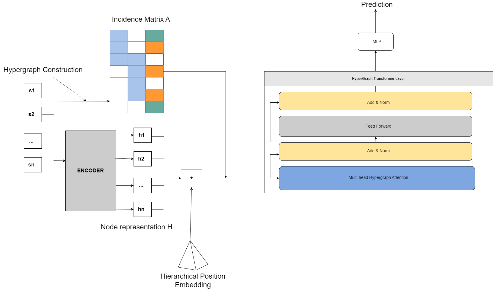
Figure 10: The overall HEGEL architecture.

5.2.3 Abstractive Summarization

Abstractive summarization is typically approached as a sequence-to-sequence language modeling task, where a neural Decoder predicts the next word of the summary at each time step. The vast majority of modern relevant methods are trained in a supervised manner, using ground-truth summaries. This is arguably a more advanced task than its extractive alternative.

5.2.3.1 Pointer-Generator Networks

One of the first truly successful abstractive summarizers is essentially a hybrid one: a DNN that dynamically chooses whether to select a source sentence verbatim, as an extractive method, or synthesize the next word in the summary [110]. Inspired by the human ability to refer to unknown objects by pointing at them, such Pointer-Generator Networks (PGNs) are an improvement over the “Word Extractor” proposed by [120].

PGN can copy out-of-vocabulary (OOV) words from the source document, making it possible to generate text with rare words and keep a smaller vocabulary, thus reducing computational and memory costs. Essentially, it is a modified, attention-augmented sequence-to-sequence Encoder-Decoder architecture implemented similarly to [121], where both the Encoder and the Decoder are one-layer, bidirectional LSTMs. The Decoder ends at a softmax layer and at each time step generates a new word, originating either in the source document or in a global supported vocabulary. Thus, at each time step of the Encoder’s/Decoder’s unfolding, the next token is read/outputted from the input/to the generated summary, respectively. In order to decide on the course of action for the next word, the PGN defines its output distribution over the union of the global and the document’s vocabulary (called the “extended vocabulary”), thus deciding at each time step whether or not it should copy or generate the next word. If a word is OOV, it will be copied from the source document by sampling from the attention distribution, while if it does not exist in the document a new word will be generated.

The attention mechanism is defined as in [46]. During inference, a coverage vector is updated at each Decoder time step, containing the sum of attention distributions over all previous time steps. It is provided as an additional input to the attention mechanism, so that the latter avoids giving attention to already extracted words and, thus, repeating them in the summary. To enhance this behaviour, PGN is also guided during training by an extra coverage loss: a regularizer that penalizes repeated attention to the same input tokens. Thus, the overall loss function computed at the $t$-th Decoder’s time step is:

$$L_{o}^{t}=L_{ML}^{t}+\lambda\sum_{i}min(a_{i}^{t},c_{i}^{t}),$$ (22)

where $\lambda$ is a scalar weighting hyperparameter, $\mathbf{a}^{t}$ is the current attention distribution, index $i$ traverses the Encoder’s time steps, $\mathbf{c}^{t}$ is the current coverage vector, while $L_{ML}^{t}$ is the primary loss term at the $t$-th Decoder’s time step. Typically, $L_{ML}^{t}$ is the negative log likelihood of the $t$-th ground-truth summary word according to the final Decoder output, i.e., a generated probability distribution defined over all supported words of the extended vocabulary. The overall loss is summed over all of the Decoder’s time steps.

PGN does not use any pretrained word embeddings, learning instead token representations from scratch. At the time of its appearance it showed remarkable success in handling OOV words, while also featuring a smaller vocabulary size and faster training times. It thus successfully handled most of the challenges outlined in Subsection 5.1. However, although historically significant, PGN cannot handle long documents well. As a result, more efficient and specialized architectures were later developed.

5.2.3.2 BERT & Sparse Attention Transformers

As described in Subsection 5.2.2, BERT has been adapted for extractive summarization in the form of BERTSUM-EXT [123]. That neural architecture has also been employed for abstractive summarization in the form of BERTSUM-ABS.

The Encoder of BERTSUM-ABS is a pretrained BERTSUM-EXT model, a choice which provides efficiency gains, due to transfer learning, and task-specific gains, due to emerging synergies between extractive and abstractive summarization [127, 128]. The Decoder is a regular, randomly initialized 6-layer Transformer. Different finetuning and training schedules are utilized for the Encoder and the Decoder, respectively, to avoid stability issues during optimization. Overall, the approach attained only marginal performance gains over competitors.

Section 4.2 reviewed the issues vanilla Transformers face with very long documents, with the biggest challenge being the quadratic cost of the self-attention mechanism. The various sparse attention solutions that attempt to bypass this restriction can also be employed for document summarization, by replacing a regular Encoder with a Sparse Transformer variant. One such architecture is the “Longformer-Encoder-Decoder” (LED), i.e., where Longformers are utilized both for the Encoder and the Decoder. Critically, the Decoder pays full attention to the entire Encoder and to already decoded positions of the input. As expected, LED scales linearly with the input size, and has been shown to achieve highly competitive performance.

Similarly, BigBird has also been employed for abstractive document summarization [90]. The sparse attention mechanism is used only in the Encoder, which handles the long input, while the Decoder exploits full attention, as the length of the summary (in tokens) is small by definition. BigBird achieved significant performance gains on long document summarization and competitive performance on smaller ones.

BigBird makes use of Gap-Sentences Generation (GSG) for abstractive summarization [129]. It is a self-supervised pretraining objective especially constructed to aid downstream finetuning for text summarization. Essentially being a variant of T5’s pretraining objective, it consists in masking an entire sentence with a single [MASK] token. Then, during pretraining, each input is a set of consecutive sentences, with a subset of them selected and hidden according to GSG. The DNN is tasked to generate the masked sentences jointly, in the form of a pseudo-summary, based on the seen ones. The selection of which input sentences to mask is not random, but based on the ROUGE score of each sentence with the remaining input text. Thus, the ones finally hidden with [MASK] tokens are those that have been automatically judged as the most important ones. It must be noted that GSG was originally introduced as the main novelty of the PEGASUS neural language model, following a Transformer Encoder-Decoder architecture, like BART or T5.

GSG and a variant of the sparse attention mechanism is also employed for abstractive document summarization in LongT5, which is a modification of the basic T5 neural architecture [130]. Thus, the LongT5 Encoder contains self-attention sublayers where each input token attends to its local neighbourhood plus to all global tokens. The latter ones are being dynamically constructed before each attention operation, by summing and normalizing different, non overlapping subsets of the input token embeddings. Despite the approximate nature of this sparse attention mechanism, the resulting ability to process longer inputs leads to overall improved accuracy in long document summarization.

5.2.3.3 Local Attention and Content Selection

The majority of modern abstractive summarizers learn to implicitly select pertinent content from the input in order to generate the summary. Recently, attempts have been made to combine the advantages of Sparse Attention Transformers, which allow the handling of longer documents, with explicit content selection before the abstractive summary generation [2].

The main abstractive DNN in [2] is a modified version of BART [57], called LoBART. Vanilla BART supports input sequences with a length up to 1024 tokens. LoBART modifies its layers so as to employ the sparse attention scheme of Longformer, with the difference that only local and no global attention is utilized. This allows LoBART to drop its memory requirements significantly, at the cost of missing context over large spans of text. The reduced costs result in a sliding window of $W=700$ tokens, which is calculated as $2\times D$ where $D$ is the empirical average attention distance of $D\in[250,350]$ tokens for an attention mechanism with uniform weights, attending to a distance of $1024$. Even with this compromise, important context may still be missed, especially in long documents.

As a result, the method in [2] feeds LoBART with suitably preprocessed input sequences, so as to effectively increase its context span. This preprocessing takes place separately during the training and the test stage. At training, the input data are first passed through a content selection algorithm. This can either be an “oracle” (ORC), which selects sentences based on the ground-truth (the ROUGE score of the selected input vs its abstract), or a hierarchical, extractive DNN pretrained for multitask content selection (MCS). The straightforward “ORC” preselection keeps an average of 21.3% of sentences, drastically reducing the input’s size and leads to 56% of the input documents being shorter than the typical BART input length of 1024. Missing sentences are padded with random sentences sampled from the input document. On the other hand, MCS is a GRU-based, attention-augmented Encoder-Decoder architecture followed by a classification layer. It employs a hierarchical design similar to that of [100] (see Section 4.2), but in this case it is only utilized to preprocess the input document. In order to exploit synergies between extractive and abstractive summarization, similarly to [123], MCS is jointly pretrained (in a multitask fashion) both for predicting the ground-truth summary token-by-token and for binary sentence classification as ”summary” or “non-summary”.

During inference, each sentence is first scored for retention by suitably combining the two different predictions (one per task) made by MCS. The top-scoring ones are fed to LoBART as the input sequence. LoBART has been trained for abstractive summarization in the usual manner, but the two-stage content preselection stage (explicit during preprocessing, implicit during the main summarization process) allows the method to efficiently handle longer documents.

5.2.3.4 Combining Top-Down and Bottom-Up Inference

An innovative abstractive methodology relying on a composite Transformer architecture is proposed in [131], aiming to facilitate the sharing of global and local context between different token representations. This is done by allowing information to flow both from the individual token representations to the document embedding (bottom-up) and vice versa (top-down).

The Encoder in [131] features a hierarchical approach similar to certain ones utilized for extractive summarization (e.g., [106]): individual token representations computed by an initial (bottom-level) deep Transformer are pooled in segments to form top-level embeddings of coarse granularity at a paragraph/section-level. This is the so-called “bottom-up” route. The preliminary top-level embeddings (one per section) are then transformed via a separate, shallow Transformer. However, the main novelty of [131] is that these final top-level representations are followingly injected to the individual token embeddings via a separate, subsequent deep“top-down” Transformer. The latter’s layers are equipped with regular self-attention, as well as with cross-attention between the top-level representations and the individual token embeddings. The final output token representations are attended by the Decoder to generate the desired abstractive summary in the usual manner.

By properly adapting Sparse Attention Transformers, the bottom-level and the top-down layers are assigned efficient local attention mechanisms only. Top-level layers can afford to be assigned full attention due to the much smaller number of sections, compared to the number of tokens. Thus, the top-down information flow enriches the lower-level embeddings with global context and the ability to capture long-range dependencies: individual token representations effectively attend to aggregated global information from the entire document, despite the local attention-only mechanisms of bottom-level layers.

The methodology is rather generic and model-agnostic, allowing it to be used with efficient Sparse Attention Transformers. This fact and the hierarchical design facilitate exceptional summarization performance in long documents, even at book-length texts. Exploring its applicability to other tasks, such as document classification, is an promising research direction.

5.2.3.5 Instruction-tuned summarization

An orthogonal direction of recent research is that of supervised finetuning of pretrained language models on “instruction” and corresponding ground-truth summary pairs. The instruction is a command to summarize in natural language, followed by the long text to be summarized. The goal is to then use, during inference, the finetuned DNN like one would use a pretrained LLM under a zero/few-shot prompting mode. This can be done both with Encoder-Decoder Transformer architectures pretrained on masked token objectives and with LLMs, which typically are Decoder-only Transformer architectures pretrained on traditional next token prediction objectives. Both T5-based architectures [132] [133] and LLM-based architectures [134] [135] [136] have recently followed this approach, typically under a multitask instruction tuning setting where text summarization is one among multiple tasks. According to common automated evaluation metrics, this approach typically leads to subpar summarization results in common public benchmarks, compared to state-of-the-art dedicated summarization DNNs. However, such summaries generated from instruction-tuned LLMs can actually be better than ones obtained from dedicated summarizers and even surpass the ground-truth ones in quality, according to manual, subjective evaluation [137]. This is a still an open area of cutting-edge research, where progress in automated evaluation metrics is a crucial prerequisite for further advances (as discussed in Subsection 5.2.1). Moreover, popular LLMs do not support well very long textual inputs.

6 Sentiment Analysis

Opinion mining (OM) or sentiment analysis (SA) is the extraction of polarity sentiment (positive/negative) from a piece of text using NLP algorithms [138, 139]. It is typically approached as a particular case of text classification, although sentiment score regression is also common [75]. Thus, possible opinions are modelled either as a set of discrete classes (e.g., “positive”, “neutral”, “negative”), or as a continuous range of sentiment scores (e.g., in the $[-1,1]$ range). Additionally, emotional dimensions besides polarity are occasionally considered (e.g., classes such as “fear”, “joy”, “sadness”, etc.), potentially by relying on psychological theory (e.g., [140]). Common use-cases mainly concern SA of short texts, such as social media posts, product reviews and online discussions, with obvious applications in marketing and brand management [141, 142, 143] or political analysis [144, 145, 146]. For an in-depth review of SA applications, the reader is referred to [147].

Long document SA is not that common; for instance, extracting the sentiment of medical or legal documents is not typically a priority, at least compared to classifying or summarizing them. However, SA can be useful for automatic analysis of long journalistic articles, to extract their political viewpoint, financial texts, to predict how markets will react to the presented news, or literary books, in order to process narrative hints. For example, it can be used to determine characters’ emotional states, or for identifying key narrative points, sections and anticipated reader feelings [30]. These predictions are potentially useful in themselves, but they can also be exploited as auxiliary input for particular book classifications tasks (e.g., automatic genre recognition in library software). Yet, the challenges faced by long document NLP constrain this to be more of a theoretical future vision, rather than a currently blooming field.

6.1 Challenges

Traditional SA algorithms rely on “sentiment lexicons”, i.e., predefined vocabularies of words that are heavily weighed towards positive or negative emotions. For example, words such as “good”, “bad”, “great”, “terrible”, etc. are likely candidates for inclusion in such as lexicon [148]. Algorithms relying on lexicons and/or traditional classifiers (e.g., Naive Bayes, SVMs, etc.) were common before the advent of DNNs [149] [150]. They are, however, limited by significant barriers that limit their performance, such as the following ones:

1. Sarcasm: As with document classification, sarcasm and figurative language cause important issues. Most SA methods falsely label a sentence in these cases, without understanding the non-literal usage of words in their specific context.

2. Inappropriate sentiment lexicons: Texts with complicated vocabulary often lack “simple” key words that are included in most lexicons. In such cases, most lexicon-based algorithms struggle to classify accurately.

3. Polysemy: It is challenging to encode semantic and syntactic relations between sentences to the semantic meaning of the document. For example, the words “contrast” and “cause” can completely flip the class of a document (see Section 4.1).

Additionally, long document SA faces challenges common to the other NLP tasks, as outlined in Sections 4.1 5.1: prohibitive computational costs, difficulty to process long input sequences, long-range dependencies that are hard to identify and sentiment variation across different sections or paragraphs.

6.2 Solutions

As expected, long document SA has moved decisively towards DNNs in the past few years. The main body of relevant research approaches the field as simply an instance of document classification, so the content of Section 4 will not be repeated here. An interesting avenue would be to exploit related short text semantic detectors of high specificity (e.g., sarcasm detectors) at the sentence-level, given that such tools are mature [151] [148] and are indeed being used to aid short text SA [75], aggregating their results in a hierarchical fashion to facilitate document-level SA. However, this research direction has not been significantly exploited. Existing deep neural methods for long text SA that offer a particular angle, compared to simple document classification, are reviewed below. The majority of these and other similar methods have not been evaluated on actually long documents, due to the lack of relevant public annotated datasets, but they can in principle support them.

6.2.1 Hybrid architectures

Initial efforts tackled documents that were a few paragraphs long, instead of book-length. For example, a composite, hierarchical deep neural architecture is proposed in [152] for classifying long user reviews (e.g., of movies, restaurants, etc.). In order to handle polysemy, the method exploits the “principle of compostitionality” [153], which states that the meaning of a body of text (a sentence, a paragraph or a document) depends on the meanings of its constituents, by using an LSTM to generate sentence-level embeddings for the entire document. These are sequentially fed to a subsequent GRU that encodes their relations and semantics, outputting a document representation that is classified by a final softmax layer. The GRU was explicitly selected due to its virtual lack of an output gate, since it was deemed necessary for all available sentence-level information to be used in the construction of the document representation. The overall architecture is trained end-to-end for classification and receives dense Word2Vec embeddings at its input layer.

A similar method [154] combines a CNN and a bidirectional LSTM to extract the sentiment of newspaper articles. It uses Doc2Vec [155] to pregenerate paragraph-level embeddings that form the input matrix for the CNN. An alternative hierarchical method is presented in [156], where an initial bidirectional LSTM sequentially receives word embeddings per sentence and transforms them to sentence embeddings. A second bidirectional LSTM equipped with an attention mechanism receives the latter representations to generate a document-level embedding in the form of a matrix, which is then fed to a final 2D CNN followed by the softmax classifier layer. As a general statement, it can be said that such straightforward hierarchical approaches (e.g., [157]) have become a de facto baseline in long text SA, with the recurrence of LSTMs typically exploited to handle the variable and large number of tokens, sentences and paragraphs in long documents.

6.2.2 Sentiment Analysis with Transformers

State-of-the-art models make use of Transformers, with BERT and its variations being very commonly used for SA [52]. The employed pretrained language model is typically finetuned on the desired SA dataset. For instance, this is how RoBERTa is utilized in [158] for SA of financial texts. However, the document-level sentiment classification task is implemented in an ensemble learning fashion, using weighted joint prediction from multiple independent classifiers, and then combined with a separate pipeline for key entity detection, so that specific entities (e.g., companies, countries, etc.) are identified in the text. Each of these entities is individually fed to an instance of an appropriately finetuned RoBERTA model (different than the SA ensemble participants) along with the document, in order for the DNN to predict whether each recognized entity is critical for its meaning.

7 Public Long Document Datasets

Long text NLP is not a well-explored field, particularly for document-level analysis of book-length texts (e.g., literary fiction). As a result, compared to small text analysis, the amount of relevant public, annotated datasets remains fairly limited. Yet, a few generic NLP datasets do include long documents. One of the most historically important ones is OntoNotes [159], which features a variety of texts and contains a number of rather long ones. OntoNotes is mainly annotated for syntax analysis tasks. Many other general-use NLP datasets include a subset of long texts, such as the OPUS dataset for machine translation [160].

Specifically long document datasets are rarer. An example would be the Project Dialogism Novel Corpus (PDNC dataset) [161], which comprises 22 English novels.

A modern large-scale dataset for literary fiction texts is LitBank [162], a dataset of 100 English literature works that fully includes word annotations and co-reference relations between words that belong in different groups. Unlike OntoNotes, it focuses particularly on long English fiction literature.

The large-scale CSL dataset [163], developed in 2022, includes a plethora of Chinese scientific literature books. Modern neural language models trained on this dataset (e.g., BERT) achieved really high accuracy in tasks such as document classification for a language as complicated as Mandarin.

Concerning document summarization, the traditionally used dataset is CNN/DailyMail [164], featuring over 330k articles and their respective highlights, as written by journalists at CNN and the Daily Mail. On average, each article has $781$ input tokens and $56$ summary (target) tokens. While the dataset is certainly large, and ships with developed and convenient APIs [165, 166, 167], its individual articles may not be long enough for modern long document summarization. This has not prevented its continuing use as a benchmark, for measuring the efficiency of contemporary summarizers in short-to-medium length documents [90].

Because of this concern, two document summarization datasets have risen into prominence the last few years: arXiv [168] [169] and PubMed [170] [171]. Both are composed of scientific research articles. They feature a huge number of documents, remarkable document length and user-curated summaries in the form of article abstracts. Their success is evident from their inclusion in many popular machine learning libraries [172] [173] [174] [175] and from their popularity as benchmarks in current document summarization literature.

Recently, two more challenging datasets have been released: BookSum [176] and SummScreen [177]. BookSum covers fiction books from multiple domains in literature, including short stories, novels and plays. SummScreen includes pairs of movie transcripts and respective human-written summaries. They both require the summarizer to combine narrative plot events from implicit subplots, potentially progressing in parallel, forcing it to rely on extremely long context spans and dependencies.

Name	Domain	Tasks	Documents	Average Document Size	Language
OntoNotes	General	Named Entity Recognition, Coreference Resolution, Semantic Role Labeling	10k-100k	-	English, Arabic, Chinese
Litbank	Literature	Named Entity Recognition	100	2000 words	English
PDNC	Literature (Old)	Quote Attribution, Speaker identification	35,978	79,745 tokens	English
CSL	Academic	Text Classification, Document Summarization, Keyword Generation (KG)	396k	-	Chinese
CNN/Daily Mail	News Articles	Document Summarization	300K	781 words	English
arXiv	Academic	Document Summarization, Text Retrieval	1.7M	-	English
Pubmed	Academic	Language Modeling, Document Classification, Document Summarization	19,717	10M-100M	English
BookSum	Literature	Text (Narrative) Summarization	146.5K paragraphs (12,6K chapters, 436 books)	-	English
SummScreen	Screenplays	Document Summarization	22,503	-	English
LexGLUE	Legal	Multiclass Document Classification	238K	-	English
MIMIC-III	Medical	Multiclass Document Classification	112K	709.3	English
ECTHR-ARG	Legal	Multiclass Document Classification	11K	-	English
ContractNLI	Legal	Multiclass Document Classification, Natural Language Inference	607	-	English
20 Newsgroup	News	Multiclass Document Classification	20k	-	English
Hyperpartisan	News	Document Classification	750K	-	English

Table 3: Reviewed long document datasets and their properties. The average document size has been noted wherever this information is publicly available.

Domain-specific datasets are crucial for domain-specific NLP algorithms, either for training or for domain finetuning [74]. Below is a brief list of such datasets, featuring primarily long documents for classification or summarization tasks:

• LexGLUE [93], a classification dataset containing a collection of smaller datasets of legal texts.

• MIMIC-III [178] (Medical Information Mart for Intensive Care), which contains Intensive Care Unit (ICU) discharge summaries. This dataset has the benefit of being annotated with labels following the ICD-9 (The International Classification of Diseases, Ninth Revision) hierarchy.

• ECtHR-ARG [179], which contains legal texts (court decisions) from the European Court of Human Rights, along with annotation for argument mining. Howev,er this dataset only contains about 300 cases.

• ContractNLI [180], a classification dataset for document-level Natural Language Inference (NLI). Each data point is a contract text and a set of hypotheses, with the three classes indicating whether each hypothesis agrees with, contradicts or is not mentioned by the contract.

• 20 Newsgroup [181], a dataset containing approximately 20,000 Usenet newsgroup documents partitioned evenly across 20 different newsgroups. This dataset provides a great amount and variety of data, but its articles tend to be significantly shorter than dedicated long document datasets.

• Hyperpartisan News Detection [182], which contains documents for political standpoint classification. This dataset contains both long and short articles, therefore a split must be performed based on the text’s length for long document analysis.

The above-mentioned datasets are summarized in Table 3.

8 Summary

This Section summarizes the issues, the existing solutions and the relevant research presented in this article. Table 4 concerns document classification and Table 5 document summarization. It must be noted that, alternatively, recent instruction-tuned LLMs (see 5.2.3) can be leveraged successfully for these tasks, but they are not explicitly designed to support long document analysis. Thus, they typically face issues with lengthy textual inputs.

Method	Addressed Issues	Details
Metrics & Preprocessing
Weighted Multi-label Classification [82]	Varying Count of Labels Per Document, Class Imbalance	By using multi-label metrics and loss functions using weighting, effective multi-label multi-class classifiers can be trained and accurately evaluated.
Feature Pruning [82, 1]	Dataset Size Computational Cost	Ruthless pruning and careful selection / sampling can significantly cut down on the computational/memory costs of long documents. On the other hand, even words traditionally considered semantically useless can be significant for a model to understand subtle grammatical and syntactical rules.
Sparse Attention Transformers
Sparse Transformers [86]	$O(n^{2})$ Transformer Cost	By utilizing a sparse attention mechanism, and with various mathematical optimizations, a standard Transformer can become viable at parsing entire long document inputs.
Dilated Sliding Window (Longformer) [87]	$O(n^{2})$ Transformer Cost Context Fragmentation	Using local self-attention with a dilated sliding window, while also allowing a limited number of global tokens, the Longformer becomes capable of successfully parsing ever-increasing-length documents, while keeping track of local context.
Sliding Window + Random Selection + Global Attention (BigBird) [90]	$O(n^{2})$ Transformer Cost Context Fragmentation	Combining Longformer’s sliding window, block attention scheme and random token selection can encapsulate local and global context more efficiently while keeping computational costs low.
Hierarchical Transformers
Hierarchical Transformers combined with traditional networks [91, 92, 97, 98]	Transformer Input Limit	Instead of using Transformers for the entire document, they can be used to produce segment embeddings, which are then combined by traditional networks (HAN, LSTM, CNN).
Hierarchical Transformers with BERT (Hi-Transformer) [99]	Global Context Context Fragmentation	BERT can be used to produce sentence embeddings, then document embeddings which can be fed to new, context-aware sentence embeddings iteratively.
Hierarchical Sparse Transformers (ERNIE-Sparse) [100]	$O(n^{2})$ Transformer Cost Local/Global Context issues	By using a hierarchical architecture embedded in a Sparse Transformer, ERNIE-SPARSE imparts token representations with additional global context.
Recurrent Transformers
Recurrent Transformers [74]	$O(n^{2})$ Transformer Cost Context Fragmentation Global Context	By keeping the context of previously inputted segments in hidden states and by utilizing relative positional embeddings, the Recurrent Transformer effectively supports much longer input sequences during inference, irrespective of training-stage sequence length.
Skimming Recurrent Transformers [101]	$O(n^{2})$ Transformer Cost Context Fragmentation Global Context Forward context	Forward and global context of greater quality can be obtained by passing through the input text twice, once by peeking small text segments (skimming phase), and then by performing a full pass (retrospective phase), fully utilizing the recurrence mechanism.

Table 4: Issues and solutions for long document classification.

Below, Table 6 presents the published scores achieved by the presented state-of-the-art methods for document summarization, in the 3 most commonly employed corresponding public datasets from Section 7. The utilized evaluation metric is ROUGE. As it can be seen, modern Sparse Transformer variants exhibit a performance advantage in long document datasets such as arXiv and PubMed, while remaining competitive in small to medium-sized datasets such as CNN/Daily Mail. Although this also seems to hold for document classification as well, it cannot be presented in the same format due to inconsistent metrics and datasets used in the relevant papers.

Method	Addressed Issues	Details
Extractive Document Summarization
Hierarchical Summarization [120, 121, 106]	DNN Use for Summarization Document Structure Under-utilization	Traditional Encoder-Decoder DNN architectures attempt to explicitly incorporate context and hierarchical elements to the features used by CNN and RNN/LSTM extractive models.
BERTSUM-Ext [164]	Poor Traditional DNN PerformanceWeaknesses in Sentence Embeddings	By using BERT as Encoder and attaching stacked Transformer layers, BERT’s expressive power leads to accurate extractive summaries.
HiStruct+ [124]	Segment/Document Context LossUnder-utilization of Document Structure	By encoding the hierarchical and topical structure of a document, the Transformer can leverage more information about rigidly structured documents (e.g., research articles).
HEGEL [125]	Under-utilization of Document Structure$O(n^{2})$ Transformer CostLong-span Dependencies	Encoding each document as a hypergraph under multiple different views leads to the model being exceptionally adept at summarizing very long and rigidly hierarchical documents.
Abstractive Document Summarization
Pointer-Generator Networks [110]	Word RepetitionVocabulary LimitationsLong Document Computational Cost	By allowing the network to choose whether to copy the next summary word from the source text or predict its own, the model can benefit from a significantly expanded vocabulary, reduce computation costs by keeping a smaller vocabulary and bypass the word repetition problem found in many extractive summarization models.
Sparse Attention Transformers [87, 90, 130]	$O(n^{2})$ Transformer Cost Vocabulary Limitations	By using a modified Sparse Transformer as the Encoder, the model can leverage the expressive power of Transformers on long documents.
Local Attention and Content Selection [2]	$O(n^{2})$ Transformer Cost Long Document Computational Cost	Pretrained models can be used for content selection in order for a Sparse Attention model to be fed only useful data, both in training and inference.

Table 5: Issues and solutions for long document summarization.

Model	CNN / Daily Mail	ArXiv	PubMed
Extractive Document Summarization
SummaRuNNer [121]	42.0	42.81	43.89
BERTSUM-Ext [164]	43.85	-	-
HiStruct+ [124]	43.65	45.22	-
HEGEL [125]	-	46.61	43.89
Abstractive Document Summarization
Pointer-Generator Networks [110]	39.53	32.06	35.86
BigBird [90]	43.84	46.63	46.32
Local Attention and Content Selection (Abstractive) [2]	-	46.59	47.47

Table 6: The ROUGE-1 scores (higher is better) for state-of-the-art extractive and abstractive summarizers on the three most popular summarization datasets (where available). These results are only indicative, since the ROUGE score’s correlation with summarization quality is under debate (see Section 5.2.1).

9 Conclusions

Analyzing long documents currently presents a daunting challenge, even with the recent NLP breakthroughs. While traditional machine learning and statistical methods provide limited functionality on these tasks, they ultimately prove less adaptable and less accurate than modern DNNs. However, the latter ones need to face long-standing issues, such as the curse of dimensionality, limited datasets, prohibitively large inputs and difficult writing formats (e.g., in literary fiction).

Most major issues are common to all long document analysis tasks and currently tend to require similar solutions, such as limiting the model’s vocabulary, modifying existing Transformer architectures to handle longer input sequences, efficiently exploiting the hierarchical structure of documents and artificially augmenting the training datasets. Task-specific solutions have also been proposed, such as using content preselection and specialized GNNs to capture long-spanning context in summarization, or passing over the input twice and using document-level representations to enrich sentence-level representations in classification. Overall, further investigation of hybrid and recurrent Transformer architectures, as well as of the top-down Transformer, seem to be promising directions for near-future improvements. Incorporation of such advances into generic LLMs is also an avenue worth exploring, along with the development of novel, improved evaluation metrics for automatic text summarization.

While this survey focuses only on document-level analysis for long texts, it becomes apparent how attempts at solving specific tasks can lead to solutions or insights with impact to all NLP fields. However, it is important to note that existing state-of-the-art solutions rely on useful trade-offs and, therefore, cannot be used universally. Finally, there is significant research potential potential for research into literary sentiment analysis, in collaboration with the digital/computational humanities community. The necessary theoretical background already exists, while the mentioned breakthroughs in long document NLP have not been yet applied.

Automated analysis of long documents is essentially a field still in its infancy, with breakthroughs leading to large jumps in computational efficiency and accuracy still frequent. Since 2015 neural network models have evolved from being constrained to (occasionally artificially) small-sized documents, to being able to effectively parse large articles and books. It is not unreasonable to expect that continuing research will help bypass most of the current limitations within the next few years.

References

- Worsham and Kalita [2018] J. Worsham, J. Kalita, Genre identification and the compositional effect of genre in literature, in: Proceedings of the International Conference on Computational Linguistics, 2018.
- Manakul and Gales [2021] P. Manakul, M. J. F. Gales, Long-span dependencies in Transformer-based summarization systems, arXiv arXiv:2105.03801 (2021).
- Nabizadeh et al. [2020] N. Nabizadeh, D. Kolossa, M. Heckmann, MyFixit: An annotated dataset, annotation tool, and baseline methods for information extraction from repair manuals, in: Proceedings of the Language Resources and Evaluation Conference, European Language Resources Association, 2020.
- Chen et al. [2022] X. Chen, P. Cong, S. Lv, A long-text classification method of chinese news based on BERT and CNN, IEEE Access 10 (2022) 34046–34057.
- Merchant and Pande [2018] K. Merchant, Y. Pande, NLP-based latent semantic analysis for legal text summarization, in: Proceedings of the IEEE International Conference on Advances in Computing, Communications and Informatics (ICACCI), 2018.
- Bongirwar [2015] V. K. Bongirwar, A survey on sentence level sentiment analysis, International Journal of Computer Science Trends and Technology (IJCST) 3 (2015) 110–113.
- Dai et al. [2015] A. M. Dai, C. Olah, Q. V. Le, Document embedding with paragraph vectors, arXiv arXiv:1507.07998 (2015).
- Ai et al. [2016] Q. Ai, L. Yang, J. Guo, W. B. Croft, Analysis of the paragraph vector model for information retrieval, in: Proceedings of the ACM International Conference on the Theory of Information Retrieval, 2016.
- Li et al. [2015] J. Li, T. Luong, D. Jurafsky, A hierarchical neural autoencoder for paragraphs and documents, in: Proceedings of the Annual Meeting of the Association for Computational Linguistics, 2015.
- Wei et al. [2020] L. Wei, D. Hu, W. Zhou, X. Tang, X. Zhang, X. Wang, J. Han, S. Hu, Hierarchical interaction networks with rethinking mechanism for document-level sentiment analysis, in: Proceedings of the European Conference on Machine Learning and Principles and Practice of Knowledge Discovery in Databases (ECML PKDD), Springer, 2020.
- Bhatia et al. [2017] S. Bhatia, J. H. Lau, T. Baldwin, An automatic approach for document-level topic model evaluation (2017).
- Bayer et al. [2023] M. Bayer, M.-A. Kaufhold, B. Buchhold, M. Keller, J. Dallmeyer, C. Reuter, Data augmentation in Natural Language Processing: a novel text generation approach for long and short text classifiers, International Journal of Machine Learning and Cybernetics 14 (2023) 135–150.
- Yogarajan et al. [2021] V. Yogarajan, J. Montiel, T. Smith, B. Pfahringer, Transformers for multi-label classification of medical text: An empirical comparison, in: Proceedings of the International Conference on Artificial Intelligence in Medicine, 2021.
- Wan et al. [2019] L. Wan, G. Papageorgiou, M. Seddon, M. Bernardoni, Long-length legal document classification, arXiv arXiv:1912.06905 (2019).
- Bambroo and Awasthi [2021] P. Bambroo, A. Awasthi, LegalDB: Long DistilBERT for legal document classification, in: Proceedings of the International Conference on Advances in Electrical, Computing, Communication and Sustainable Technologies (ICAECT), 2021.
- Dale [2019] R. Dale, Law and word order: NLP in legal tech, Natural Language Engineering 25 (2019) 211–217.
- Blei et al. [2003] D. M. Blei, A. Y. Ng, M. I. Jordan, Latent Dirichlet Allocation, Journal of Machine Learning Research 3 (2003) 993–1022.
- Webster and Kit [1992] J. J. Webster, C. Kit, Tokenization as the initial phase in NLP, in: Proceedings of the International Conference on Computational Linguistics (COLING), 1992.
- Sidorov et al. [2014] G. Sidorov, F. Velasquez, E. Stamatatos, A. Gelbukh, L. Chanona-Hernández, Syntactic N-grams as machine learning features for Natural Language Processing, Expert Systems with Applications 41 (2014) 853–860.
- Korde and Mahender [2012] V. Korde, C. N. Mahender, Text classification and classifiers: A survey, International Journal of Artificial Intelligence & Applications 3 (2012) 85.
- Kowsari et al. [2019] K. Kowsari, K. Jafari Meimandi, M. Heidarysafa, S. Mendu, L. Barnes, D. Brown, Text classification algorithms: A survey, Information 10 (2019).
- Torfi et al. [2020] A. Torfi, R. A. Shirvani, Y. Keneshloo, N. Tavaf, E. A. Fox, Natural Language Processing advancements by deep learning: A survey, arXiv arXiv:2003.01200 (2020).
- Chai and Li [2019] J. Chai, A. Li, Deep learning in Natural Language Processing: A state-of-the-art survey, in: Proceedings of the International Conference on Machine Learning and Cybernetics (ICMLC), 2019.
- Schröder and Niekler [2020] C. Schröder, A. Niekler, A survey of active learning for text classification using Deep Neural Networks, arXiv arXiv:2008.07267 (2020).
- Li et al. [2022] Q. Li, H. Peng, J. Li, C. Xia, R. Yang, L. Sun, P. S. Yu, L. He, A survey on text classification: From traditional to deep learning, ACM Transactions on Intelligent Systems and Technology 13 (2022).
- Gupta and Gupta [2019] S. Gupta, S. K. Gupta, Abstractive summarization: An overview of the state of the art, Expert Systems with Applications 121 (2019) 49–65.
- Hussein [2018] D. M. E.-D. M. Hussein, A survey on sentiment analysis challenges, Journal of King Saud University-Engineering Sciences 30 (2018) 330–338.
- Wagh et al. [2021] V. Wagh, S. Khandve, I. Joshi, A. Wani, G. Kale, R. Joshi, Comparative study of long document classification, in: Proceedings of the IEEE Region 10 Conference (TENCON), 2021.
- Koh et al. [2022] H. Y. Koh, J. Ju, M. Liu, S. Pan, An empirical survey on long document summarization: Datasets, models, and metrics, ACM Computing Surveys 55 (2022) 1–35.
- Mori et al. [2022] Y. Mori, H. Yamane, Y. Mukuta, T. Harada, Computational storytelling and emotions: A survey, arXiv arXiv:2003.01200 (2022).
- Alshuwaier et al. [2022] F. Alshuwaier, A. Areshey, J. Poon, Applications and enhancement of document-based sentiment analysis in deep learning methods: Systematic literature review, Intelligent Systems with Applications 15 (2022) 200090.
- Rumelhart [1986] D. E. Rumelhart, Learning internal representations by error propagation, in parallel distributed processing, MIT press, 1986, pp. 318–362.
- Jordan [1997] M. I. Jordan, Serial order: A parallel distributed processing approach 121 (1997) 471–495.
- Lecun et al. [1998] Y. Lecun, L. Bottou, Y. Bengio, P. Haffner, Gradient-based learning applied to document recognition, Proceedings of the IEEE 86 (1998) 2278–2324.
- Krizhevsky et al. [2017] A. Krizhevsky, I. Sutskever, G. E. Hinton, ImageNet classification with deep Convolutional Neural Networks, Communications of the ACM 60 (2017) 84––90.
- Huynh-The et al. [2020] T. Huynh-The, C.-H. Hua, J.-W. Kim, S.-H. Kim, D.-S. Kim, Exploiting a low-cost CNN with skip connection for robust automatic modulation classification, in: Proceedings of the IEEE Wireless Communications and Networking Conference (WCNC), 2020.
- Russakovsky et al. [2015] O. Russakovsky, J. Deng, H. Su, J. Krause, S. Satheesh, S. Ma, Z. Huang, A. Karpathy, A. Khosla, M. Bernstein, et al., ImageNet large scale visual recognition challenge, International Journal of Computer Vision 115 (2015) 211–252.
- Yang et al. [2018] Y.-X. Yang, C. Wen, K. Xie, F.-Q. Wen, G.-Q. Sheng, X.-G. Tang, Face recognition using the SR-CNN model, Sensors 18 (2018).
- Kayalibay et al. [2017] B. Kayalibay, G. Jensen, P. van der Smagt, CNN-based segmentation of medical imaging data, arXiv preprint arXiv:1701.03056 (2017).
- Dauphin et al. [2017] Y. N. Dauphin, A. Fan, M. Auli, D. Grangier, Language modeling with gated convolutional networks, in: International conference on machine learning, PMLR, 2017.
- Siegelmann and Sontag [1991] H. T. Siegelmann, E. D. Sontag, Turing computability with neural nets, Applied Mathematics Letters 4 (1991) 77–80.
- Hochreiter and Schmidhuber [1997] S. Hochreiter, J. Schmidhuber, Long Short-Term Memory, Neural computation 9 (1997) 1735–80.
- Calin [2020] O. Calin, Deep Learning Architectures, Springer, 2020.
- Graves et al. [2013] A. Graves, A. Rahman Mohamed, G. E. Hinton, Speech recognition with deep Recurrent Neural Networks, in: Proceedings of the IEEE International Conference on Acoustics, Speech and Signal Processing (ICASSP), 2013.
- Cho et al. [2014] K. Cho, B. Van Merriënboer, D. Bahdanau, Y. Bengio, On the properties of neural machine translation: Encoder-Decoder approaches, arXiv arXiv:1409.1259 (2014).
- Bahdanau et al. [2015] D. Bahdanau, K. Cho, Y. Bengio, Neural Machine Translation by jointly learning to align and translate, in: Proceedings of the International Conference on Learning Representations (ICLR), 2015.
- Vaswani et al. [2017] A. Vaswani, N. Shazeer, N. Parmar, J. Uszkoreit, L. Jones, A. N. Gomez, L. Kaiser, I. Polosukhin, Attention is all you need, in: Proceedings of the Advances in Neural Information Processing Systems (NIPS), 2017.
- Mikolov et al. [2013] T. Mikolov, K. Chen, G. Corrado, J. Dean, Efficient estimation of word representations in vector space, arXiv preprint arXiv:1301.3781 (2013).
- Jurafsky and Martin [2000] D. Jurafsky, J. H. Martin, Speech and Language Processing, Pearson, 2000.
- Pennington et al. [2014] J. Pennington, R. Socher, C. Manning, GloVe: Global vectors for word representation, in: Proceedings of the Conference on Empirical Methods in Natural Language Processing (EMNLP), Association for Computational Linguistics, 2014.
- Peters et al. [2018] M. E. Peters, M. Neumann, M. Iyyer, M. Gardner, C. Clark, K. Lee, L. Zettlemoyer, Deep contextualized word representations, in: Proceedings of the Conference of the North American Chapter of the Association for Computational Linguistics, 2018.
- Devlin et al. [2019] J. Devlin, M.-W. Chang, K. Lee, K. Toutanova, BERT: Pre-training of deep bidirectional Transformers for language understanding, in: Proceedings of the Conference of the North American Chapter of the Association for Computational Linguistics: Human Language Technologies, Volume 1 (Long and Short Papers), Association for Computational Linguistics, 2019.
- Taylor [1953] W. L. Taylor, “cloze procedure”: A new tool for measuring readability, Journalism Quarterly 30 (1953) 415–433.
- Liu et al. [2019] Y. Liu, M. Ott, N. Goyal, J. Du, M. Joshi, D. Chen, O. Levy, M. Lewis, L. Zettlemoyer, V. Stoyanov, RoBERTa: A robustly optimized BERT pretraining approach, arXiv arXiv:1907.11692 (2019).
- Clark et al. [2020] K. Clark, M. Luong, Q. V. Le, C. D. Manning, ELECTRA: pre-training text encoders as discriminators rather than generators, in: Proceedings of the International Conference on Learning Representations (ICLR), 2020.
- Raffel et al. [2020] C. Raffel, N. Shazeer, A. Roberts, K. Lee, S. Narang, M. Matena, Y. Zhou, W. Li, P. J. Liu, Exploring the limits of transfer learning with a unified text-to-text transformer, The Journal of Machine Learning Research 21 (2020) 5485–5551.
- Lewis et al. [2019] M. Lewis, Y. Liu, N. Goyal, M. Ghazvininejad, A. Mohamed, O. Levy, V. Stoyanov, L. Zettlemoyer, BART: denoising sequence-to-sequence pre-training for natural language generation, translation and comprehension, arXiv arXiv:1910.13461 (2019).
- Tay et al. [2022] Y. Tay, M. Dehghani, V. Q. Tran, X. Garcia, J. Wei, X. Wang, H. W. Chung, D. Bahri, T. Schuster, S. e. a. Zheng, UL2: Unifying language learning paradigms, in: Proceedings of the International Conference on Learning Representations (ICLR), 2022.
- Radford et al. [2018a] A. Radford, K. Narasimhan, T. Salimans, I. Sutskever, Improving language understanding by generative pre-training, 2018a.
- Radford et al. [2018b] A. Radford, J. Wu, R. Child, D. Luan, D. Amodei, I. Sutskever, Language models are unsupervised multitask learners, 2018b.
- Tan et al. [????] B. Tan, Z. Yang, A.-S. Maruan, E. P. Xing, Z. Hu, Progressive generation of long text, arXiv arXiv:2006.15720 (????).
- Chowdhery et al. [2022] A. Chowdhery, S. Narang, J. Devlin, M. Bosma, G. Mishra, A. Roberts, P. Barham, H. W. Chung, C. Sutton, S. e. a. Gehrmann, PaLM: Scaling language modeling with pathways, arXiv preprint arXiv:2204.02311 (2022).
- Scao et al. [2022] T. L. Scao, A. Fan, C. Akiki, E. Pavlick, S. Ilić, D. Hesslow, R. Castagné, A. S. Luccioni, F. Yvon, M. e. a. Gallé, BLOOM: A 176B-parameter open-access multilingual language model, arXiv preprint arXiv:2211.05100 (2022).
- Zhang et al. [2022] S. Zhang, S. Roller, N. Goyal, M. Artetxe, M. Chen, S. Chen, C. Dewan, M. Diab, X. Li, X. V. e. a. Lin, OPT: Open pre-trained transformer language models, arXiv preprint arXiv:2205.01068 (2022).
- Hoffmann et al. [2022] J. Hoffmann, S. Borgeaud, A. Mensch, E. Buchatskaya, T. Cai, E. Rutherford, D. de Las Casas, L. A. Hendricks, J. Welbl, A. e. a. Clark, An empirical analysis of compute-optimal large language model training, Proceedings of the Advances in Neural Information Processing Systems (NIPS) (2022).
- Touvron et al. [2023] H. Touvron, T. Lavril, G. Izacard, X. Martinet, M.-A. Lachaux, T. Lacroix, B. Rozière, N. Goyal, E. Hambro, F. e. a. Azhar, LLaMA: Open and efficient foundation language models, arXiv preprint arXiv:2302.13971 (2023).
- Chalkidis et al. [2019] C. Chalkidis, M. Fergadiotis, P. Malakasiotis, I. Androutsopoulos, Large-scale multi-label text classification on EU legislation, in: Proceedings of the Annual Meeting of the Association for Computational Linguistics, 2019.
- Chalkidis et al. [2020] I. Chalkidis, M. Fergadiotis, S. Kotitsas, P. Malakasiotis, N. Aletras, I. Androutsopoulos, An empirical study on large-scale multi-label text classification including few and zero-shot labels, Proceedings of the Conference on Empirical Methods in Natural Language Processing (2020).
- Zhang et al. [2020] N. Zhang, Q. Jia, K. Yin, L. Dong, F. Gao, N. Hua, Conceptualized representation learning for chinese biomedical text mining, arXiv arXiv:2008.10813 (2020).
- Khadhraoui et al. [2022] M. Khadhraoui, H. Bellaaj, M. B. Ammar, H. Hamam, M. Jmaiel, Survey of BERT-based models for scientific text classification: COVID-19 case study, Applied Sciences 12 (2022).
- Lee et al. [2019] J. Lee, W. Yoon, S. Kim, D. Kim, S. Kim, C. H. So, J. Kang, BioBERT: a pre-trained biomedical language representation model for biomedical text mining, Bioinformatics 36 (2019) 1234–1240.
- Chen et al. [2022] H. Chen, L. Wu, J. Chen, W. Lu, J. Ding, A comparative study of automated legal text classification using random forests and deep learning, Information Processing & Management 59 (2022) 102798.
- Worsham [2014] J. M. Worsham, Towards Literary Genre Identification: Applied Neural Networks for Large Text Classification, University of Colorado, 2014.
- Dai et al. [2022] X. Dai, I. Chalkidis, S. Darkner, D. Elliott, Revisiting Transformer-based models for long document classification, in: Proceedings of the Findings of the Association for Computational Linguistics (EMNLP), 2022.
- Karamouzas et al. [2022] D. Karamouzas, I. Mademlis, I. Pitas, Neural knowledge transfer for sentiment analysis in texts with figurative language, in: Proceedings of the IEEE International Workshop on Machine Learning for Signal Processing (MLSP), 2022.
- Monte-Serrat et al. [2021] D. M. Monte-Serrat, M. T. Machado, E. E. S. Ruiz, A machine learning approach to literary genre classification on portuguese texts: circumventing NLP’s standard varieties, in: Anais do XIII Simpósio Brasileiro de Tecnologia da Informação e da Linguagem Humana, SBC, 2021.
- I. [2020] T. I., Development and application of language models in Greek literature, 2020. doi:10.26262/heal.auth.ir.323350.
- Russell and Norvig [2016] S. Russell, P. Norvig, Artificial Intelligence: A Modern Approach, Pearson Education, Upper Saddle River, New Jersey 07458, 2016.
- Cortes and Vapnik [1995] C. Cortes, V. Vapnik, Support-vector networks, Machine Learning 20 (1995) 273–297.
- Quinlan [1994] J. R. Quinlan, S.L. C4.5: Programs for Machine Learning, Morgan Kaufmann Publishers, Upper Saddle River, New Jersey 07458, 1994.
- Xu et al. [2012] B. Xu, X. Guo, Y. Ye, J. Cheng, An improved random forest classifier for text categorization, Journal of King Saud University - Computer and Information Sciences 7 (2012) 2913–2920.
- Liu et al. [2020] S. Liu, Z. Huang, Y. Li, Z. Sun, J. Wu, H. Zhang, DeepGenre: Deep neural networks for genre classification in literary works, 2020.
- Hsu et al. [2020] C.-C. Hsu, P.-C. Chang, A. Chang, Multi-label classification of icd coding using deep learning, in: Proceedings of the IEEE International Symposium on Community-centric Systems (CcS), 2020.
- Haghighian Roudsari et al. [2022] A. Haghighian Roudsari, J. Afshar, W. Lee, S. Lee, PatentNet: multi-label classification of patent documents using deep learning-based language understanding, Scientometrics (2022) 1–25.
- Kim [2014] Y. Kim, Convolutional Neural Networks for sentence classification, in: Proceedings of the Conference on Empirical Methods in Natural Language Processing (EMNLP), 2014.
- Child et al. [2019] R. Child, S. Gray, A. Radford, I. Sutskever, Generating long sequences with Sparse Transformers, arXiv arXiv:1904.10509 (2019).
- Beltagy et al. [2020] I. Beltagy, M. Peters, A. Cohan, Longformer: The long-document Transformer, arXiv arXiv:2004.05150 (2020).
- Saeed et al. [2020] H. A. Saeed, H. Wang, M. Peng, A. Hussain, A. Nawaz, Online fault monitoring based on Deep Neural Network & sliding window technique, Progress in Nuclear Energy 121 (2020) 103236.
- Krystalakos et al. [2018] O. Krystalakos, C. Nalmpantis, D. Vrakas, Sliding window approach for online energy disaggregation using Artificial Neural Networks, in: Proceedings of the Hellenic Conference on Artificial Intelligence (SETN), 2018.
- Zaheer et al. [2020] M. Zaheer, G. Guruganesh, K. A. Dubey, J. Ainslie, C. Alberti, S. Ontanon, P. Pham, A. Ravula, Q. Wang, L. e. a. Yang, Big Bird: Transformers for longer sequences, in: Proceedings of the Advances in Neural Information Processing Systems (NIPS), 2020.
- Chalkidis et al. [2019] I. Chalkidis, I. Androutsopoulos, N. Aletras, Neural legal judgment prediction in English, in: Proceedings of the Annual Meeting of the Association for Computational Linguistics (ACL), 2019.
- Yang et al. [2016] Z. Yang, D. Yang, C. Dyer, X. He, A. Smola, E. Hovy, Hierarchical Attention Networks for document classification, in: Proceedings of the Conference of the North American Chapter of the Association for Computational Linguistics: Human Language Technologies, 2016.
- Chalkidis et al. [2021] I. Chalkidis, A. Jana, D. Hartung, M. Bommarito, I. Androutsopoulos, D. Katz, N. Aletras, LexGLUE: A benchmark dataset for legal language understanding in English (2021).
- Chen et al. [2020] Y. Chen, Y. Sun, Z. Yang, H. Lin, Joint entity and relation extraction for legal documents with legal feature enhancement, in: Proceedings of the International Conference on Computational Linguistics, 2020.
- Chalkidis et al. [2020] I. Chalkidis, M. Fergadiotis, P. Malakasiotis, N. Aletras, I. Androutsopoulos, LEGAL-BERT: The Muppets straight out of law school, in: Proceedings of the Conference on Empirical Methods in Natural Language Processing (EMNLP), 2020.
- Zheng et al. [2021] L. Zheng, N. Guha, B. R. Anderson, P. Henderson, D. E. Ho, When does pretraining help? assessing self-supervised learning for law and the casehold dataset of 53,000+ legal holdings, in: Proceedings of the International Conference on Artificial Intelligence and Law, 2021.
- Khandve et al. [2022] S. I. Khandve, V. K. Wagh, A. D. Wani, I. M. Joshi, R. B. Joshi, Hierarchical neural network approaches for long document classification, in: Proceedings of the International Conference on Machine Learning and Computing (ICMLC), 2022.
- Cer et al. [2018] D. Cer, Y. Yang, S.-Y. Kong, N. Hua, N. Limtiaco, R. S. John, N. Constant, M. Guajardo-Cespedes, S. Yuan, C. e. a. Tar, Universal sentence encoder, arXiv arXiv:1803.11175 (2018).
- Wu et al. [2021] C. Wu, F. Wu, T. Qi, Y. Huang, Hi-Transformer: Hierarchical interactive Transformer for efficient and effective long document modeling, in: Proceedings of the Annual Meeting of the Association for Computational Linguistics and the International Joint Conference on Natural Language Processing, 2021.
- Liu et al. [2022] Y. Liu, J. Liu, L. Chen, Y. Lu, S. Feng, Z. Feng, Y. Sun, H. Tian, H. Wu, H. Wang, ERNIE-SPARSE: Learning hierarchical efficient Transformer through regularized self-attention, 2022.
- Dai et al. [2019] Z. Dai, Z. Yang, Y. Yang, J. Carbonell, Q. Le, R. Salakhutdinov, Transformer-XL: Attentive language models beyond a fixed-length context, in: Proceedings of the Annual Meeting of the Association for Computational Linguistics, 2019.
- Ding et al. [2021] S. Ding, J. Shang, S. Wang, Y. Sun, H. Tian, H. Wu, H. Wang, ERNIE-Doc: A retrospective long-document modeling transformer, in: Proceedings of the Annual Meeting of the Association for Computational Linguistics and the International Joint Conference on Natural Language Processing, 2021.
- Mehta [2016] P. Mehta, From extractive to abstractive summarization: A journey, in: Proceedings of the ACL Student Research Workshop, 2016.
- Cho et al. [2014] K. Cho, B. van Merrienboer, C. Gülçehre, F. Bougares, H. Schwenk, y. Bengio, Learning phrase representations using RNN encoder-decoder for statistical machine translation, Proceedings of the Conference on Empirical Methods in Natural Language Processing (EMNLP) (2014).
- Sutskever et al. [2014] I. Sutskever, O. Vinyals, Q. V. Le, Sequence to sequence learning with neural networks, in: Z. Ghahramani, M. Welling, C. Cortes, N. Lawrence, K. Weinberger (Eds.), Proceedings of the Advances in Neural Information Processing Systems (NIPS), 2014.
- Xiao and Carenini [2019] W. Xiao, G. Carenini, Extractive summarization of long documents by combining global and local context, in: Proceedings of the Conference on Empirical Methods in Natural Language Processing and the International Joint Conference on Natural Language Processing (EMNLP-IJCNLP), Association for Computational Linguistics, 2019.
- Lin [2004] C.-Y. Lin, ROUGE: A package for automatic evaluation of summaries, in: Text Summarization Branches Out, Association for Computational Linguistics, 2004.
- Akter et al. [2022] M. Akter, N. Bansal, S. K. Karmaker, Revisiting automatic evaluation of extractive summarization task: Can we do better than ROUGE?, in: Proceedings of the Findings of the Association for Computational Linguistics (ACL), 2022.
- Zhong et al. [2020] M. Zhong, P. Liu, Y. Chen, D. Wang, X. Qiu, X. Huang, Extractive summarization as text matching, 2020.
- See et al. [2017] A. See, P. J. Liu, C. D. Manning, Get to the point: Summarization with Pointer-Generator Networks, arXiv preprint arXiv:1704.04368 (2017).
- Suleiman and Awajan [2020] D. Suleiman, A. Awajan, Deep learning-based abstractive text summarization: approaches, datasets, evaluation measures, and challenges, Mathematical problems in engineering 2020 (2020) 1–29.
- Graham [2015] Y. Graham, Re-evaluating automatic summarization with BLEU and 192 shades of ROUGE, in: Proceedings of the Conference on Empirical Methods in Natural Language Processing (EMNLP), 2015.
- Pitler et al. [2010] E. Pitler, A. Louis, A. Nenkova, Automatic evaluation of linguistic quality in multi-document summarization, in: Proceedings of the Annual Meeting of the Association for Computational Linguistics, 2010.
- Fabbri et al. [2021] A. R. Fabbri, W. Kryściński, B. McCann, C. Xiong, R. Socher, D. Radev, SummEval: Re-evaluating summarization evaluation, Transactions of the Association for Computational Linguistics 9 (2021) 391–409.
- Kryscinski et al. [2020] W. Kryscinski, B. McCann, C. Xiong, R. Socher, Evaluating the factual consistency of abstractive text summarization, in: Proceedings of the Conference on Empirical Methods in Natural Language Processing (EMNLP), 2020.
- Banerjee and Lavie [2005] S. Banerjee, A. Lavie, METEOR: An automatic metric for MT evaluation with improved correlation with human judgments, in: Proceedings of the ACL Workshop on Intrinsic and Extrinsic Evaluation Measures for Machine Translation and/or Summarization, Association for Computational Linguistics, 2005.
- Zhang et al. [2020] T. Zhang, V. Kishore, F. Wu, K. Q. Weinberger, Y. Artzi, BERTScore: Evaluating text generation with BERT, in: Proceedings of the International Conference on Learning Representations (ICLR), 2020.
- Peyrard et al. [2017] M. Peyrard, T. Botschen, I. Gurevych, Learning to score system summaries for better content selection evaluation, in: Proceedings of the Workshop on New Frontiers in Summarization, 2017.
- Vasilyev et al. [2020] O. Vasilyev, V. Dharnidharka, J. Bohannon, Fill in the BLANC: human-free quality estimation of document summaries (2020).
- Cheng and Lapata [2016] J. Cheng, M. Lapata, Neural summarization by extracting sentences and words, in: Proceedings of the Annual Meeting of the Association for Computational Linguistics, Association for Computational Linguistics, 2016.
- Nallapati et al. [2016] R. Nallapati, F. Zhai, B. Zhou, SummaRuNNer: A Recurrent Neural Network-based sequence model for extractive summarization of documents, in: Proceedings of the AAAI Conference on Artificial Intelligence, 2016.
- Wang and Chang [2016] W. Wang, B. Chang, Graph-based dependency parsing with bidirectional LSTM, in: Proceedings of the Annual Meeting of the Association for Computational Linguistics (Volume 1: Long Papers), Association for Computational Linguistics, 2016.
- Liu and Lapata [2019] Y. Liu, M. Lapata, Text summarization with pretrained encoders, in: Proceedings of the Conference on Empirical Methods in Natural Language Processing and the International Joint Conference on Natural Language Processing (EMNLP-IJCNLP), 2019.
- Ruan et al. [2022] Q. Ruan, M. Ostendorff, G. Rehm, HiStruct+: Improving extractive text summarization with hierarchical structure information, arXiv arXiv:2203.09629 (2022).
- Zhang et al. [2022] H. Zhang, X. Liu, J. Zhang, HEGEL: Hypergraph Transformer for long document summarization, in: Proceedings of the Conference on Empirical Methods in Natural Language Processing (EMNLP), 2022.
- Grootendorst [2020] M. Grootendorst, KeyBERT: Minimal keyword extraction with BERT, 2020. URL: https://doi.org/10.5281/zenodo.4461265. doi:10.5281/zenodo.4461265.
- Li et al. [2018] W. Li, X. Xiao, Y. Lyu, Y. Wang, Improving neural abstractive document summarization with explicit information selection modeling, in: Proceedings of the Conference on Empirical Methods in Natural Language Processing (EMNLP), 2018.
- Gehrmann et al. [2018] S. Gehrmann, Y. Deng, A. Rush, Bottom-up abstractive summarization, in: Proceedings of the Conference on Empirical Methods in Natural Language Processing (EMNLP), 2018.
- Zhang et al. [2020] J. Zhang, Y. Zhao, M. Saleh, P. Liu, PEGASUS: Pre-training with extracted gap-sentences for abstractive summarization, in: Proceedings of the International Conference on Machine Learning (ICML), PMLR, 2020.
- Guo et al. [2022] M. Guo, J. Ainslie, D. Uthus, S. Ontanon, J. Ni, Y.-H. Sung, Y. Yang, LongT5: Efficient text-to-text transformer for long sequences, in: Proceedings of the Annual Conference of the North American Chapter of the Association for Computational Linguistics (NAAC), 2022.
- Pang et al. [2023] B. Pang, E. Nijkamp, W. Kryściński, S. Savarese, Y. Zhou, C. Xiong, Long document summarization with top-down and bottom-up inference, in: Proceedings of the Findings of the Association for Computational Linguistics (ACL), 2023.
- Victor et al. [2022] S. Victor, W. Albert, R. Colin, B. Stephen, S. Lintang, A. Zaid, C. Antoine, S. Arnaud, R. Arun, D. e. a. Manan, Multitask prompted training enables zero-shot task generalization, in: Proceedings of the International Conference on Learning Representations (ICLR), 2022.
- Chung et al. [2022] H. W. Chung, L. Hou, S. Longpre, B. Zoph, Y. Tay, W. Fedus, E. Li, X. Wang, M. Dehghani, S. e. a. Brahma, Scaling instruction-finetuned language models, arXiv preprint arXiv:2210.11416 (2022).
- Ouyang et al. [2022] L. Ouyang, J. Wu, X. Jiang, D. Almeida, C. Wainwright, P. Mishkin, C. Zhang, S. Agarwal, K. Slama, A. e. a. Ray, Training language models to follow instructions with human feedback, Proceedings of the Advances in Neural Information Processing Systems (NIPS) (2022).
- Iyer et al. [2022] S. Iyer, X. V. Lin, R. Pasunuru, T. Mihaylov, D. Simig, P. Yu, K. Shuster, T. Wang, Q. Liu, P. S. e. a. Koura, OPT-IML: Scaling language model instruction meta learning through the lens of generalization, arXiv preprint arXiv:2212.12017 (2022).
- Muennighoff et al. [2022] N. Muennighoff, T. Wang, L. Sutawika, A. Roberts, S. Biderman, T. L. Scao, M. S. Bari, S. Shen, Z.-X. Yong, H. e. a. Schoelkopf, Cross-lingual generalization through multitask finetuning, arXiv preprint arXiv:2211.01786 (2022).
- Goyal et al. [2022] T. Goyal, J. J. Li, G. Durrett, News summarization and evaluation in the era of GPT-3, arXiv preprint arXiv:2209.12356 (2022).
- Ahmad and Edalati [2022] W. Ahmad, M. Edalati, Urdu speech and text based sentiment analyzer, arXiv preprint arXiv:2207.09163 (2022).
- Barreto et al. [2023] S. Barreto, R. Moura, J. Carvalho, A. Paes, A. Plastino, Sentiment analysis in tweets: an assessment study from classical to modern word representation models, Data Mining and Knowledge Discovery 37 (2023) 318–380.
- Plutchik [2001] R. Plutchik, The nature of emotions: Human emotions have deep evolutionary roots, a fact that may explain their complexity and provide tools for clinical practice, American scientist 89 (2001) 344–350.
- Rambocas and Pacheco [2018] M. Rambocas, B. G. Pacheco, Online sentiment analysis in marketing research: a review, Journal of Research in Interactive Marketing (2018).
- Rambocas et al. [2013] M. Rambocas, J. Gama, et al., Marketing research: The role of sentiment analysis, Technical Report, Universidade do Porto, Faculdade de Economia do Porto, 2013.
- Micu et al. [2017] A. Micu, A. E. Micu, M. Geru, R. C. Lixandroiu, Analyzing user sentiment in social media: Implications for online marketing strategy, Psychology & Marketing 34 (2017) 1094–1100.
- Ramteke et al. [2016] J. Ramteke, S. Shah, D. Godhia, A. Shaikh, Election result prediction using Twitter sentiment analysis, in: Proceedings of the International Conference on Inventive Computation Technologies (ICICT), 2016.
- Kaya et al. [2012] M. Kaya, G. Fidan, I. H. Toroslu, Sentiment analysis of Turkish political news, in: Proceedings of the IEEE/WIC/ACM International Conferences on Web Intelligence and Intelligent Agent Technology, 2012.
- Karamouzas et al. [2022] D. Karamouzas, I. Mademlis, I. Pitas, Public opinion monitoring through collective semantic analysis of tweets, Social Network Analysis and Mining 12 (2022) 91.
- Drus and Khalid [2019] z. Drus, H. Khalid, Sentiment analysis in social media and its application: Systematic literature review, Procedia Computer Science 161 (2019) 707–714.
- Mehndiratta et al. [2017] P. Mehndiratta, S. Sachdeva, D. Soni, Detection of sarcasm in text data using deep convolutional neural networks, Scalable Computing: Practice and Experience 18 (2017) 219–228.
- Pang et al. [2002] B. Pang, L. Lee, S. Vaithyanathan, Thumbs up? sentiment classification using machine learning techniques, in: Proceedings of the Conference on Empirical Methods in Natural Language Processing (EMNLP), Association for Computational Linguistics, 2002.
- Pang and Lee [2004] B. Pang, L. Lee, A sentimental education: Sentiment analysis using subjectivity summarization based on minimum cuts, in: Proceedings of the Annual Meeting on Association for Computational Linguistics (ACL ’04), Association for Computational Linguistics, 2004.
- Davidov et al. [2010] D. Davidov, O. Tsur, A. Rappoport, Semi-supervised recognition of sarcasm in Twitter and Amazon, in: Proceedings of the Conference on Computational Natural Language Learning, 2010.
- Tang et al. [2015] D. Tang, B. Qin, T. Liu, Document modeling with Gated Recurrent Neural Network for sentiment classification, in: Proceedings of the Conference on Empirical Methods in Natural Language Processing, Association for Computational Linguistics, 2015.
- Pelletier [1994] F. Pelletier, The principle of semantic compositionality, Topoi 13 (1994) 11–24.
- Rhanoui et al. [2019] M. Rhanoui, M. Mikram, S. Yousfi, S. Barzali, A CNN-BiLSTM model for document-level sentiment analysis, Machine Learning and Knowledge Extraction 1 (2019) 832–847.
- Le and Mikolov [2014] Q. Le, T. Mikolov, Distributed representations of sentences and documents, in: Proceedings of the International Conference on Machine Learning, PMLR, 2014.
- Mao et al. [2022] Y. Mao, Y. Zhang, L. Jiao, H. Zhang, Document-level sentiment analysis using attention-based bi-directional Long Short-Term Memory network and two-dimensional Convolutional Neural Network, Electronics 11 (2022) 1906.
- Bhuvaneshwari et al. [2022] P. Bhuvaneshwari, A. N. Rao, Y. H. Robinson, M. Thippeswamy, Sentiment analysis for user reviews using Bi-LSTM self-attention-based CNN model, Multimedia Tools and Applications 81 (2022) 12405–12419.
- Zhao et al. [2020] L. Zhao, L. Li, X. Zheng, J. Zhang, A BERT-based sentiment analysis and key entity detection approach for on-line financial texts, in: Proceedings of the IEEE International Conference on Computer Supported Cooperative Work in Design (CSCWD), 2020.
- Weischedel et al. [2011] R. Weischedel, E. Hovy, M. Marcus, M. Palmer, R. Belvin, S. Pradhan, L. Ramshaw, N. Xue, OntoNotes: A Large Training Corpus for Enhanced Processing, 2011.
- Tiedemann [2012] J. Tiedemann, Parallel data, tools and interfaces in OPUS, in: Proceedings of the International Conference on Language Resources and Evaluation (LREC), European Language Resources Association (ELRA), 2012.
- Vishnubhotla et al. [2022] K. Vishnubhotla, A. Hammond, G. Hirst, The Project Dialogism Novel Corpus: A dataset for quotation attribution in literary texts, arXiv preprint arXiv:2204.05836 (2022).
- Bamman et al. [2020] D. Bamman, O. Lewke, A. Mansoor, An annotated dataset of coreference in English literature, in: Proceedings of the International Conference on Language Resources and Evaluation (LREC), European Language Resources Association, 2020.
- Li et al. [2022] Y. Li, Y. Zhang, Z. Zhao, L. Shen, W. Liu, W. Mao, H. Zhang, CSL: A large-scale Chinese scientific literature dataset, arXiv preprint arXiv:2209.05034 (2022).
- Nallapati et al. [2016] R. Nallapati, B. Zhou, C. dos Santos, C. Gulcehre, B. Xiang, Abstractive text summarization using sequence-to-sequence RNNs and beyond, in: Proceedings of the SIGNLL Conference on Computational Natural Language Learning, 2016.
- tf_[date] TensorFlow CNN-DailyMail Dataset, https://www.tensorflow.org/datasets/catalog/cnn_dailymail, nodate. Accessed: 2023-05-30.
- kag [date] Kaggle CNN-DailyMail Dataset, https://www.kaggle.com/datasets/gowrishankarp/newspaper-text-summarization-cnn-dailymail, nodate. Accessed: 2023-05-30.
- hug [date] Hugging Face CNN-DailyMail Dataset, https://pan.webis.de/data.html#pan-semeval-hyperpartisan-news-detection-19, nodate. Accessed: 2023-05-30.
- Clement et al. [2019] C. B. Clement, M. Bierbaum, K. P. O’Keeffe, A. A. Alemi, On the use of arXiv as a dataset, arXiv arXiv:1905.00075 (2019).
- Gong et al. [2016] J. Gong, X. Chen, X. Qiu, X. Huang, End-to-end neural sentence ordering using pointer network, arXiv arXiv:1611.04953 (2016).
- Gupta et al. [2021] V. Gupta, P. Bharti, P. Nokhiz, H. Karnick, SumPubMed: Summarization dataset of PubMed scientific articles, in: Proceedings of the Annual Meeting of the Association for Computational Linguistics and the International Joint Conference on Natural Language Processing: Student Research Workshop, 2021.
- Dernoncourt and Lee [2017] F. Dernoncourt, J. Y. Lee, PubMed 200k RCT: a dataset for sequential sentence classification in medical abstracts, arXiv arXiv:1710.06071 (2017).
- tf-datasets [date] tf-datasets, TensorFlow scientific papers dataset, https://www.tensorflow.org/datasets/catalog/scientific_papers, nodate. Accessed: 2023-04-22.
- Bozsolik [2020] T. Bozsolik, Kaggle arXiv dataset, https://www.tensorflow.org/datasets/catalog/scientific_papers, 2020. Accessed: 2023-04-22.
- arxiv-hugging-face [date] arxiv-hugging-face, Hugging Face library arXiv dataset, https://www.tensorflow.org/datasets/catalog/scientific_papers, nodate. Accessed: 2023-04-22.
- pubmed-hugging-face [date] pubmed-hugging-face, Hugging Face library arXiv dataset, https://huggingface.co/datasets/pubmed, nodate. Accessed: 2023-04-22.
- Kryściński et al. [2022] W. Kryściński, N. Rajani, D. Agarwal, C. Xiong, D. Radev, BookSum: A collection of datasets for long-form narrative summarization, in: Proceedings of the Findings of the Association for Computational Linguistics (ACL), 2022.
- Chen et al. [2021] M. Chen, Z. Chu, S. Wiseman, K. Gimpel, SummScreen: A dataset for abstractive screenplay summarization, 2021.
- Johnson et al. [2016] A. E. Johnson, T. J. Pollard, L. Shen, L.-W. H. Lehman, M. Feng, M. Ghassemi, B. Moody, P. Szolovits, L. Anthony Celi, R. G. Mark, MIMIC-III, a freely accessible critical care database, Scientific Data 3 (2016) 1–9.
- Habernal et al. [2023] I. Habernal, D. Faber, N. Recchia, S. Bretthauer, I. Gurevych, I. Spiecker genannt Döhmann, C. Burchard, Mining legal arguments in court decisions, Artificial Intelligence and Law (2023) 1–38.
- Koreeda and Manning [2021] Y. Koreeda, C. Manning, ContractNLI: A dataset for document-level natural language inference for contracts, in: Proceedings of the Findings of the Association for Computational Linguistics (EMNLP), 2021.
- 20 Groups [date] 20 Groups, 20 newsgroups, http://qwone.com/~jason/20Newsgroups/, nodate. Accessed: 2023-04-30.
- Hyperpartisan [date] Hyperpartisan, Hyperpartisan dataset, https://pan.webis.de/data.html#pan-semeval-hyperpartisan-news-detection-19, nodate. Accessed: 2023-04-30.